Load Flow Studies

Overview

Load flow studies are one of the most important aspects of power system planning and operation. The load flow gives us the sinusoidal steady state of the entire system - voltages, real and reactive power generated and absorbed and line losses. Since the load is a static quantity and it is the power that flows through transmission lines, the purists prefer to call this Power Flow studies rather than load flow studies. We shall however stick to the original nomenclature of load flow.

Through the load flow studies we can obtain the voltage magnitudes and angles at each bus in the steady state. This is rather important as the magnitudes of the bus voltages are required to be held within a specified limit. Once the bus voltage magnitudes and their angles are computed using the load flow, the real and reactive power flow through each line can be computed. Also based on the difference between power flow in the sending and receiving ends, the losses in a particular line can also be computed. Furthermore, from the line flow we can also determine the over and under load conditions.

The steady state power and reactive power supplied by a bus in a power network are expressed in terms of nonlinear algebraic equations. We therefore would require iterative methods for solving these equations. In this chapter we shall discuss two of the load flow methods. We shall also delineate how to interpret the load flow results.

Section I: Real And Reactive Power Injected in a Bus

For the formulation of the real and reactive power entering a b us, we need to define the following quantities. Let the voltage at the i th bus be denoted by

Also let us define the self admittance at bus- i as

(4.1)

mywbut.com

1

Similarly the mutual admittance between the buses i and j can be written as

Let the power system contains a total number of n buses. The current injected at bus- i is given as

It is to be noted we shall assume the current entering a bus to be positive and that leaving the bus to be negative. As a consequence the power and reactive power entering a bus will also be assumed to be positive. The complex power at bus- i is then given by

Note that

(4.2)

(4.3)

(4.4)

(4.5)

mywbut.com

2

Therefore substituting in (4.5) we get the real and reactive power as

Section II: Classification Of Buses

For load flow studies it is assumed that the loads are constant and they are defined by their real and reactive power consumption. It is further assumed that the generator terminal voltages are tightly regulated and therefore are constant. The main objective of the load flow is to find the voltage magnitude of each bus and its angle when the powers generated and loads are pre-specified. To facilitate this we classify the different buses of the power system shown in the chart below.

Load Buses : In these buses no generators are connected and hence the generated real power PGi and reactive power QGi are taken as zero. The load drawn by these buses are defined by real power -PLi and reactive power -QLi in which the negative sign accommodates for the power flowing out of the bus. This is why these buses are sometimes referred to as P-Q bus. The objective of the load flow is to find the bus voltage magnitude |Vi| and its angle δi.

(4.6)

(4.7)

mywbut.com

3

Voltage Controlled Buses : These are the buses where generators are connected. Therefore the power generation in such buses is controlled through a prime mover while the terminal voltage is controlled through the generator excitation. Keeping the input power constant through turbine-governor control and keeping the bus voltage constant using automatic voltage regulator, we can specify constant PGi and | Vi | for these buses. This is why such buses are also referred to as P-V buses. It is to be noted that the reactive power supplied by the generator QGi depends on the system configuration and cannot be specified in advance. Furthermore we have to find the unknown angle δi of the bus voltage.

Slack or Swing Bus : Usually this bus is numbered 1 for the load flow studies. This bus sets the angular reference for all the other buses. Since it is the angle difference between two voltage sources that dictates the real and reactive power flow between them, the particular angle of the slack bus is not important. However it sets the reference against which angles of all the other bus voltages are measured. For this reason the angle of this bus is usually chosen as 0° . Furthermore it is assumed that the magnitude of the voltage of this bus is known.

Now consider a typical load flow problem in which all the load demands are known. Even if the generation matches the sum total of these demands exactly, the mismatch between generation and load will persist because of the line I 2R losses. Since the I 2R loss of a line depends on the line current which, in turn, depends on the magnitudes and angles of voltages of the two buses connected to the line, it is rather difficult to estimate the loss without calculating the voltages and angles. For this reason a generator bus is usually chosen as the slack bus without specifying its real power. It is assumed that the generator connected to this bus will supply the balance of the real power required and the line losses.

Section III: Preparation Of Data For Load Flow

Let real and reactive power generated at bus- i be denoted by PGi and QGi respectively. Also let us denote the real and reactive power consumed at the i th th bus by PLi and QLi respectively. Then the net real power injected in bus- i is

Let the injected power calculated by the load flow program be Pi, calc . Then the mismatch between the actual injected and calculated values is given by

(4.8)

mywbut.com

4

In a similar way the mismatch between the reactive power injected and calculated values is given by

The purpose of the load flow is to minimize the above two mismatches. It is to be noted that (4.6) and (4.7) are used for the calculation of real and reactive power in (4.9) and (4.10). However since the magnitudes of all the voltages and their angles are not known a priori, an iterative procedure must be used to estimate the bus voltages and their angles in order to calculate the mismatches. It is expected that mismatches ΔPi and ΔQi reduce with each iteration and the load flow is said to have converged when the mismatches of all the buses become less than a very small number.

For the load flow studies we shall consider the system of Fig. 4.1, which has 2 generator and 3 load buses. We define bus-1 as the slack bus while taking bus-5 as the P-V bus. Buses 2, 3 and 4 are P-Q buses. The line impedances and the line charging admittances are given in Table 4.1. Based on this data the Y bus matrix is given in Table 4.2. This matrix is formed using the same procedure as given in Section 3.1.3. It is to be noted here that the sources and their internal impedances are not considered while forming the Ybus matrix for load flow studies which deal only with the bus voltages.

Fig. 4.1 The simple power system used for load flow studies.

(4.9)

(4.10)

mywbut.com

5

Table 4.1 Line impedance and line charging data of the system of Fig. 4.1.

Line (bus to bus) Impedance Line charging ( Y /2) 1-2 0.02 + j 0.10 j 0.030 1-5 0.05 + j 0.25 j 0.020 2-3 0.04 + j 0.20 j 0.025 2-5 0.05 + j 0.25 j 0.020 3-4 0.05 + j 0.25 j 0.020 3-5 0.08 + j 0.40 j 0.010 4-5 0.10 + j 0.50 j 0.075

Table 4.2 Ybus matrix of the system of Fig. 4.1.

1 2 3 4 5 1 2.6923 - j 13.4115 - 1.9231 + j

9.6154 0 0 - 0.7692 + j

3.8462 2 - 1.9231 + j

9.6154 3.6538 - j 18.1942 - 0.9615 + j

4.8077 0 - 0.7692 + j

3.8462 3 0 - 0.9615 + j

4.8077 2.2115 - j 11.0027 - 0.7692 + j

3.8462 - 0.4808 + j

2.4038 4 0 0 - 0.7692 + j

3.8462 1.1538 - j 5.6742 - 0.3846 + j

1.9231 5 - 0.7692 + j

3.8462 - 0.7692 + j

3.8462 - 0.4808 + j

2.4038 - 0.3846 + j

1.9231 2.4038 - j 11.8942

The bus voltage magnitudes, their angles, the power generated and consumed at each bus are given in Table 4.3. In this table some of the voltages and their angles are given in boldface letters. This indicates that these are initial data used for starting the load flow program. The power and reactive power generated at the slack bus and the reactive power generated at the P-V bus are unknown. Therefore each of these quantities are indicated by a dash ( - ). Since we do not need these quantities for our load flow calculations, their initial estimates are not required. Also note from Fig. 4.1 that the slack bus does not contain any load while the P-V bus 5 has a local load and this is indicated in the load column.

mywbut.com

6

Table 4.3 Bus voltages, power generated and load - initial data.

Bus no. Bus voltage Power generated Load Magnitude (pu) Angle (deg) P (MW) Q (MVAr) P (MW) P (MVAr) 1 1.05 0 - - 0 0 2 1 0 0 0 96 62 3 1 0 0 0 35 14 4 1 0 0 0 16 8 5 1.02 0 48 - 24 11

Section IV: Load Flow by Gauss-Seidel Method

The basic power flow equations (4.6) and (4.7) are nonlinear. In an n -bus power system, let the number of P-Q buses be np and the number of P-V (generator) buses be ng such that n = np + ng + 1. Both voltage magnitudes and angles of the P-Q buses and voltage angles of the P-V buses are unknown making a total number of 2np + ng quantities to be determined. Amongst the known quantities are 2np numbers of real and reactive powers of the P-Q buses, 2ng numbers of real powers and voltage magnitudes of the P-V buses and voltage magnitude and angle of the slack bus. Therefore there are sufficient numbers of known quantities to obtain a solution of the load flow problem. However, it is rather difficult to obtain a set of closed form equations from (4.6) and (4.7). We therefore have to resort to obtain iterative solutions of the load flow problem.

At the beginning of an iterative method, a set of values for the unknown quantities are chosen. These are then updated at each iteration. The process continues till errors between all the known and actual quantities reduce below a pre-specified value. In the Gauss-Seidel load flow we denote the initial voltage of the i th bus by Vi

(0) , i = 2, ... , n . This should read as the voltage of the i th bus at the 0th iteration, or initial guess. Similarly this voltage after the first iteration will be denoted by Vi

(1) . In this Gauss-Seidel load flow the load buses and voltage controlled buses are treated differently. However in both these type of buses we use the complex power equation given in (4.5) for updating the voltages. Knowing the real and reactive power injected at any bus we can expand (4.5) as

We can rewrite (4.11) as

(4.11)

mywbut.com

7

In this fashion the voltages of all the buses are updated. We shall outline this procedure with the help of the system of Fig. 4.1, with the system data given in Tables 4.1 to 4.3. It is to be noted that the real and reactive powers are given respectively in MW and MVAr. However they are converted into per unit quantities where a base of 100 MVA is chosen.

Updating Load Bus Voltages

Let us start the procedure with bus-2 of the 5 bus 7 line system given in fig: 4.1. Since this is load bus, both the real and reactive power into this bus is known. We can therefore write from (4.12)

From the data given in Table 4.3 we can write

It is to be noted that since the real and reactive power is drawn from this bus, both these quantities appear in the above equation with a negative sign. With the values of the Y bus elements given in Table 4.2 we get V2

1 = 0.9927 < − 2.5959° .

The first iteration voltage of bus-3 is given by

(4.12)

(4.13)

mywbut.com

8

Note that in the above equation since the update for the bus-2 voltage is already available, we used the 1st iteration value of this rather than the initial value. Substituting the numerical data we get V3

(1) = 0.9883 < − 2. 8258° . Finally the bus-4 voltage is given by

Solving we get V4(1) = 0. 9968 < −3.4849° .

Updating P-V Bus Voltages

It can be seen from Table 4.3 that even though the real power is specified for the P-V bus-5, its reactive power is unknown. Therefore to update the voltage of this bus, we must first estimate the reactive power of this bus. Note from Fig. 4.11 that

And hence we can write the kth iteration values as

(4.14)

(4.15)

(4.16)

(4.17)

mywbut.com

9

For the system of Fig. 4.1 we have

This is computed as 0.0899 per unit. Once the reactive power is estimated, the bus-5 voltage is updated as

It is to be noted that even though the power generation in bus-5 is 48 MW, there is a local load that is consuming half that amount. Therefore the net power injected by this bus is 24 MW and consequently the injected power P5, inj in this case is taken as 0.24 per unit. The voltage is calculated as V5

(1) = 1.0169 < − 0.8894° . Unfortunately however the magnitude of the voltage obtained above is not equal to the magnitude given in Table 4.3. We must therefore force this voltage magnitude to be equal to that specified. This is accomplished by

This will fix the voltage magnitude to be 1.02 per unit while retaining the phase of − 0.8894 ° . The corrected voltage is used in the next iteration.

Convergence of the Algorithm

As can be seen from Table 4.3 that a total number of 4 real and 3 reactive powers are known to us. We must then calculate each of these from (4.6) and (4.7) using the values of the voltage magnitudes and their angle obtained after each iteration. The power mismatches are then

(4.18)

(4.19)

(4.20)

mywbut.com

10

calculated from (4.9) and (4.10). The process is assumed to have converged when each of ΔP2 , ΔP3, ΔP4 , ΔP5 , ΔQ2 , ΔQ3 and ΔQ4 is below a small pre-specified value. At this point the process is terminated.

Sometimes to accelerate computation in the P-Q buses the voltages obtained from (4.12) is multiplied by a constant. The voltage update of bus- i is then given by

where λ is a constant that is known as the acceleration factor . The value of λ has to be below 2.0 for the convergence to occur. Table 4.4 lists the values of the bus voltages after the 1st iteration and number of iterations required for the algorithm to converge for different values of λ. It can be seen that the algorithm converges in the least number of iterations when λ is 1.4 and the maximum number of iterations are required when λ is 2. In fact the algorithm will start to diverge if larger values of acceleration factor are chosen. The system data after the convergence of the algorithm will be discussed later.

Table 4.4 Gauss-Seidel method: bus voltages after 1 st iteration and number of iterations required for convergence for different values of l .

λ Bus voltages (per unit) after 1st iteration No of iterations

for convergence V2 V3 V4 V5

1 0.9927∠− 2.6° 0.9883∠− 2.83° 0.9968∠− 3.48° 1.02 ∠− 0.89° 28 2 0.9874∠− 5.22° 0.9766∠− 8.04° 0.9918∠− 14.02° 1.02∠− 4.39° 860

1.8 0.9883∠− 4.7° 0.9785∠− 6.8° 0.9903∠− 11.12° 1.02∠− 3.52° 54 1.6 0.9893∠− 4.17° 0.9807∠− 5.67° 0.9909∠− 8.65° 1.02∠− 2.74° 24 1.4 0.9903∠− 3.64° 0.9831∠− 4.62° 0.9926∠− 6.57° 1.02∠− 2.05° 14 1.2 0.9915∠− 3.11° 0.9857∠− 3.68° 0.9947∠− 4.87° 1.02∠− 1.43° 19

(4.21)

mywbut.com

11

Section V: Solution of a Set of Nonlinear Equations by Newton-Raphson Method

In this section we shall discuss the solution of a set of nonlinear equations through Newton-Raphson method. Let us consider that we have a set of n nonlinear equations of a total number of n variables x1 , x2 , ... , xn. Let these equations be given by

where f1, ... , fn are functions of the variables x1 , x2 , ... , xn. We can then define another set of functions g1 , ... , gn as given below

Let us assume that the initial estimates of the n variables are x1(0) , x2

(0) , ... , xn(0) . Let us add

corrections Δx1(0) , Δx2

(0) , ... , Δxn(0) to these variables such that we get the correct solution of

these variables defined by

(4.22)

(4.23)

(4.24)

mywbut.com

12

The functions in (4.23) then can be written in terms of the variables given in (4.24) as

We can then expand the above equation in Taylor 's series around the nominal values of x1(0) ,

x2(0) , ... , xn

(0) . Neglecting the second and higher order terms of the series, the expansion of gk , k = 1, ... , n is given as

where is the partial derivative of gk evaluated at x2(1) , ... , xn

(1) .

Equation (4.26) can be written in vector-matrix form as

The square matrix of partial derivatives is called the Jacobian matrix J with J (1) indicating that the matrix is evaluated for the initial values of x2

(0) , ... , xn(0) . We can then write the solution of

(4.27) as

(4.25)

(4.26)

(4.27)

mywbut.com

13

Since the Taylor 's series is truncated by neglecting the 2nd and higher order terms, we cannot expect to find the correct solution at the end of first iteration. We shall then have

These are then used to find J (1) and Δgk (1) , k = 1, ... , n . We can then find Δx2(1) , ... , Δxn

(1) from an equation like (4.28) and subsequently calculate x2

(1) , ... , xn(1). The process continues till Δgk ,

k = 1, ... , n becomes less than a small quantity.

(4.28)

(4.29)

mywbut.com

14

Section VI: Load Flow By Newton-Raphson Method

• Load Flow Algorithm • Formation of the Jacobian Matrix • Solution of Newton-Raphson Load Flow

Let us assume that an n -bus power system contains a total np number of P-Q buses while the number of P-V (generator) buses be ng such that n = np + ng + 1. Bus-1 is assumed to be the slack bus. We shall further use the mismatch equations of ΔPi and ΔQi given in (4.9) and (4.10) respectively. The approach to Newton-Raphson load flow is similar to that of solving a system of nonlinear equations using the Newton-Raphson method: At each iteration we have to form a Jacobian matrix and solve for the corrections from an equation of the type given in (4.27). For the load flow problem, this equation is of the form

where the Jacobian matrix is divided into submatrices as

It can be seen that the size of the Jacobian matrix is ( n + np − 1) x ( n + np −1). For example for the 5-bus problem of Fig. 4.1 this matrix will be of the size (7 x 7). The dimensions of the submatrices are as follows:

J11: (n − 1) × (n − 1), J12: (n − 1) × np, J21: np × (n − 1) and J22: np × np

(4.30)

(4.31)

mywbut.com

15

The submatrices are

Load Flow Algorithm

The Newton-Raphson procedure is as follows:

Step-1: Choose the initial values of the voltage magnitudes |V| (0) of all np load buses and n − 1 angles δ (0) of the voltages of all the buses except the slack bus.

Step-2: Use the estimated |V|(0) and δ (0) to calculate a total n − 1 number of injected real power Pcalc

(0) and equal number of real power mismatch ΔP (0) .

(4.32)

(4.33)

(4.34)

(4.35)

mywbut.com

16

Step-3: Use the estimated |V| (0) and δ (0) to calculate a total np number of injected reactive power Qcalc

(0) and equal number of reactive power mismatch ΔQ (0) .

Step-3: Use the estimated |V| (0) and δ (0) to formulate the Jacobian matrix J (0) .

Step-4: Solve (4.30) for δ (0) and Δ |V| (0) ÷ |V| (0).

Step-5 : Obtain the updates from

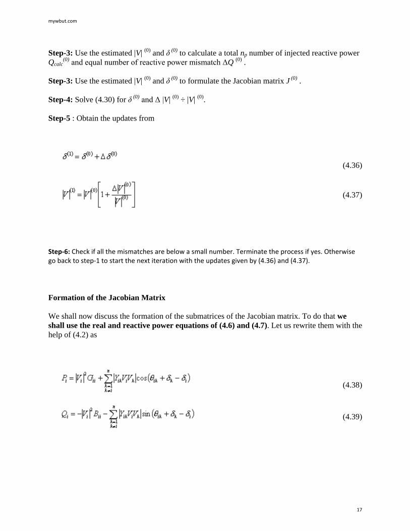
Step-6: Check if all the mismatches are below a small number. Terminate the process if yes. Otherwise go back to step-1 to start the next iteration with the updates given by (4.36) and (4.37).

Formation of the Jacobian Matrix

We shall now discuss the formation of the submatrices of the Jacobian matrix. To do that we shall use the real and reactive power equations of (4.6) and (4.7). Let us rewrite them with the help of (4.2) as

(4.36)

(4.37)

(4.38)

(4.39)

mywbut.com

17

A. Formation of J11

Let us define J11 as

It can be seen from (4.32) that Lik's are the partial derivatives of Pi with respect to δk. The derivative Pi (4.38) with respect to k for i ≠ k is given by

Similarly the derivative Pi with respect to k for i = k is given by

Comparing the above equation with (4.39) we can write

(4.40)

(4.41)

(4.42)

mywbut.com

18

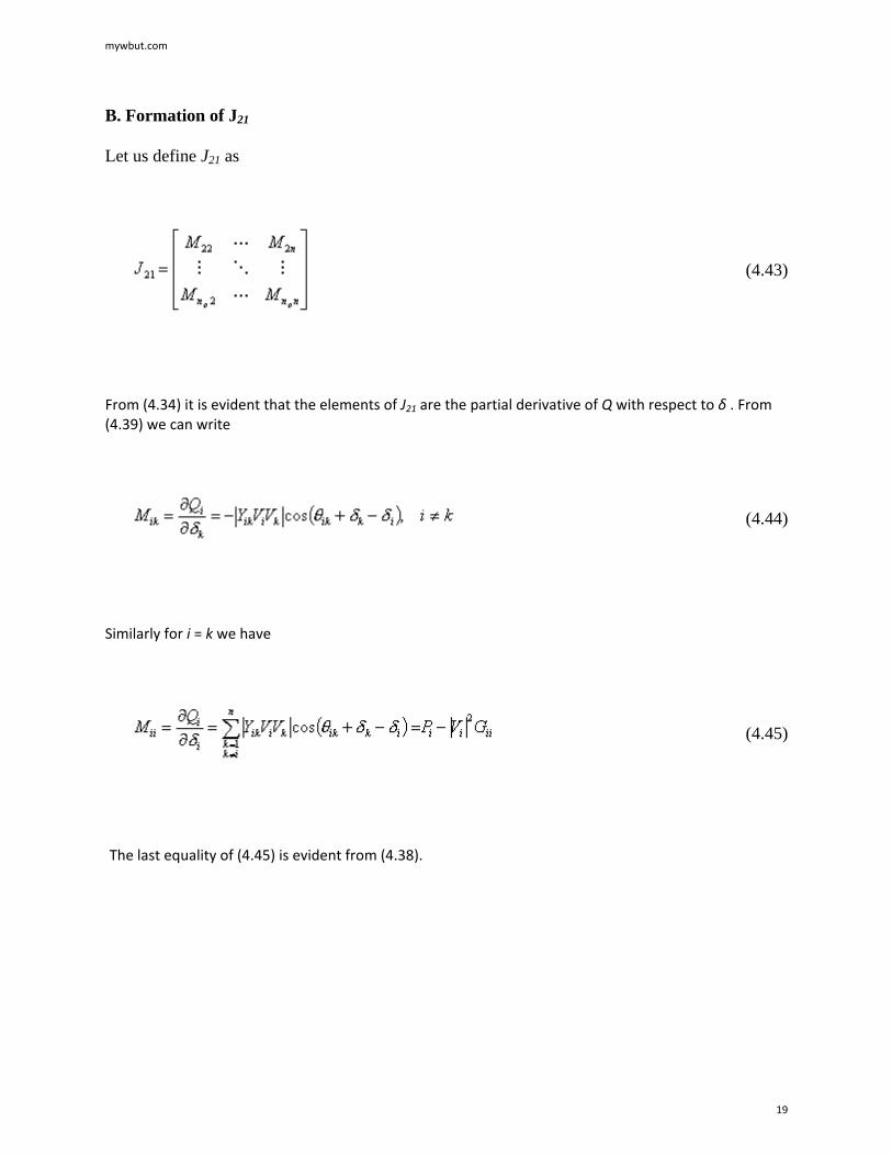
B. Formation of J21

Let us define J21 as

From (4.34) it is evident that the elements of J21 are the partial derivative of Q with respect to δ . From (4.39) we can write

Similarly for i = k we have

The last equality of (4.45) is evident from (4.38).

(4.43)

(4.44)

(4.45)

mywbut.com

19

C. Formation of J12

Let us define J12 as

As evident from (4.33), the elements of J21 involve the derivatives of real power P with respect to magnitude of bus voltage |V| . For i ≠ k , we can write from (4.38)

For i = k we have

(4.46)

(4.47)

(4.48)

mywbut.com

20

Formation of J22

For the formation of J22 let us define

For i ≠ k we can write from (4.39)

Finally for i = k we have

We therefore see that once the submatrices J11 and J21 are computed, the formation of the submatrices J12 and J22 is fairly straightforward. For large system this will result in considerable saving in the computation time.

(4.49)

(4.50)

(4.51)

mywbut.com

21

Solution of Newton-Raphson Load Flow

The Newton-Raphson load flow program is tested on the system of Fig. 4.1 with the system data and initial conditions given in Tables 4.1 to 4.3. From (4.41) we can write

Similarly from (4.39) we have

Hence from (4.42) we get

In a similar way the rest of the components of the matrix J11(0) are calculated. This matrix is given by

For forming the off diagonal elements of J21 we note from (4.44) that

Also from (4.38) the real power injected at bus-2 is calculated as

Hence from (4.45) we have

Similarly the rest of the elements of the matrix J21 are calculated. This matrix is then given as

mywbut.com

22

For calculating the off diagonal elements of the matrix J12 we note from (4.47) that they are negative of the off diagonal elements of J21 . However the size of J21 is (3 X 4) while the size of J12 is (4 X 3). Therefore to avoid this discrepancy we first compute a matrix M that is given by

The elements of the above matrix are computed in accordance with (4.44) and (4.45). We can then define

Furthermore the diagonal elements of J12 are overwritten in accordance with (4.48). This matrix is then given by

Finally it can be noticed from (4.50) that J22 = J11 (1:3, 1:3). However the diagonal elements of J22 are then overwritten in accordance with (4.51). This gives the following matrix

From the initial conditions the power and reactive power are computed as

mywbut.com

23

Consequently the mismatches are found to be

Then the updates at the end of the first iteration are given as

The load flow converges in 7 iterations when all the power and reactive power mismatches are below 10−6 .

Section VII: Load Flow Results

In this section we shall discuss the results of the load flow. It is to be noted here that both Gauss-Seidel and Newton-Raphson methods yielded the same result. However the Newton-Raphson method converged faster than the Gauss-Seidel method. The bus voltage magnitudes, angles of each bus along with power generated and consumed at each bus are given in Table 4.4. It can be seen from this table that the total power generated is 174.6 MW whereas the total load is 171 MW. This indicates that there is a line loss of about 3.6 MW for all the lines put together. It is to be noted that the real and reactive power of the slack bus and the reactive power of the P-V bus are computed from (4.6) and (4.7) after the convergence of the load flow.

Table 4.4 Bus voltages, power generated and load after load flow convergence.

Bus no.

Bus voltage Power generated Load Magnitude (pu) Angle (deg) P (MW) Q (MVAr) P (MW) P (MVAr)

1 1.05 0 126.60 57.11 0 0

2 0.9826 − 5.0124 0 0 96 62

mywbut.com

24

3 0.9777 − 7.1322 0 0 35 14

4 0.9876 − 7.3705 0 0 16 8

5 1.02 − 3.2014 48 15.59 24 11

The current flowing between the buses i and k can be written as

Therefore the complex power leaving bus- i is given by

Similarly the complex power entering bus- k is

Therefore the I 2 R loss in the line segment i-k is

The real power flow over different lines is listed in Table 4.5. This table also gives the I2 R loss along various segments. It can be seen that all the losses add up to 3.6 MW, which is the net difference

(4.52)

(4.53)

(4.54)

(4.55)

mywbut.com

25

between power generation and load. Finally we can compute the line I2X drops in a similar fashion. This drop is given by

However we have to consider the effect of line charging separately.

Table 4.5 Real power flow over different lines.

Power dispatched Power received Line loss (MW)

from (bus) amount (MW) in (bus) amount (MW) 1 101.0395 2 98.6494 2.3901 1 25.5561 5 25.2297 0.3264 2 17.6170 3 17.4882 0.1288 3 0.7976 4 0.7888 0.0089 5 15.1520 2 14.9676 0.1844 5 18.6212 3 18.3095 0.3117 5 15.4566 4 15.2112 0.2454

Total = 3.5956

Consider the line segment 1-2. The voltage of bus-1 is V1 = 1.05 < 0° per unit while that of bus-2 is V2 = 0.9826 < − 5.0124° per unit. From (4.52) we then have

per unit

Therefore the complex power dispatched from bus-1 is

where the negative signal indicates the power is leaving bus-1. The complex power received at bus-2 is

MW

(4.56)

mywbut.com

26

Therefore out of a total amount of 101.0395 MW of real power is dispatched from bus-1 over the line segment 1-2, 98.6494 MW reaches bus-2. This indicates that the drop in the line segment is 2.3901 MW. Note that

MW

where R12 is resistance of the line segment 1-2. Therefore we can also use this method to calculate the line loss.

Now the reactive drop in the line segment 1-2 is

MV Ar

We also get this quantity by subtracting the reactive power absorbed by bus-2 from that supplied by bus-1. The above calculation however does not include the line charging. Note that since the line is modeled by an equivalent- p , the voltage across the shunt capacitor is the bus voltage to which the shunt capacitor is connected. Therefore the current I 12 flowing through line segment is not the current leaving bus-1 or entering bus-2 - it is the current flowing in between the two charging capacitors. Since the shunt branches are purely reactive, the real power flow does not get affected by the charging capacitors. Each charging capacitor is assumed to inject a reactive power that is the product of the half line charging admittance and square of the magnitude of the voltage of that at bus. The half line charging admittance of this line is 0.03. Therefore line charging capacitor will inject

MV Ar

at bus-1. Similarly the reactive injected at bus-2 will be

MV Ar

The power flow through the line segments 1-2 and 1-5 are shown in Fig. 4.2.

(a)

mywbut.com

27

(b)

Fig. 4.2 Real and reactive power flow through (a) line segment 1-2 and (b) line segment 1-5. The thin lines indicate reactive power flow while the thick lines indicate real power flow.

mywbut.com

28