Embed Size (px)
Citation preview

Load Balancing
• How?– Partition the computation into units of work (tasks or jobs)– Assign tasks to different processors
• Load Balancing Categories– Static (load assigned before application runs)– Dynamic (load assigned as applications run)
o Centralized (Tasks assigned by the master or root process)o De-centralized (Tasks reassigned among slaves)
– Semi-dynamic (application periodically suspended and load balanced)
• Load Balancing Algorithms are:– Adaptive if they adapt to different system load levels
o Thresholds control how they adapt– Stable if load balancing traffic is independent of load levels– Symmetric if both senders and receivers initiate action– Effective if load balancing overhead is minimal
A load is balanced if no processes are idle

Improving the Load Balance
By realigning processing work, we improve speed-up

Static Load Balancing
• Round Robin – Tasks given to processes
in sequential order.– If there are more tasks
than processors, the allocation wraps around to the first
• Randomized– Tasks are assigned
randomly to processors• Partitioning – Tasks
represented by a graph– Recursive Bisection– Simulated Annealing– Genetic Algorithms– Multi-level Contraction
and Refinement
• Advantage– Simple to implement– Minimal run time
overhead• Disadvantages
– Predicting execution times is often not knowable before execution
– Affect of communication dynamics is often not considered
– The number of iterations is often indeterminate
Done prior to executing the parallel application

Dynamic Load Balancing
• Centralized– A single process hands out tasks– Processes ask for more work when their processing completes– Double buffering can be effective
• Decentralized– Processes detect that their work load is low– Processes can sense an overload condition
• This occurs when new tasks are spawned during execution– Questions
• Which neighbors are part of the rebalancing?• How should thresholds be set?• What are the communications needed to balance?• How often should balancing occur?
Done as a parallel application executes

Centralized Load Balancing
Master ProcessorWhile ( task=Remove()) != null)
Receive(pi, request_msg)
Send(pi, task)While(more processes)
Receive(pi, request_msg)
Send(pi, termination_msg)
Slave Processortask = Receive(pmaster, message)While (task!=terminate) Process task
Send(pmaster, request_msg)
task = Receive(pmaster, message)
Work Pool, Processer Farm, or Replicated Worker Algorithm
Slaves
Master
In this case, the slaves don’t spawn new tasks
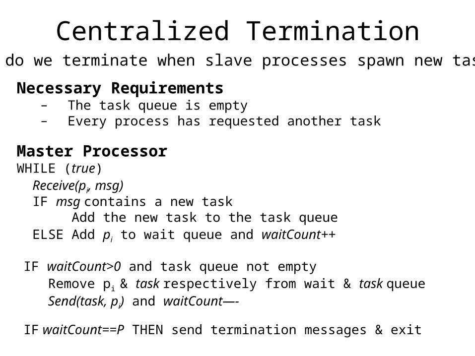
Centralized Termination
Necessary Requirements– The task queue is empty– Every process has requested another task
Master ProcessorWHILE (true) Receive(pi, msg) IF msg contains a new task Add the new task to the task queue ELSE Add pi to wait queue and waitCount++
IF waitCount>0 and task queue not empty Remove pi & task respectively from wait & task queue Send(task, pi) and waitCount—-
IF waitCount==P THEN send termination messages & exit
How do we terminate when slave processes spawn new tasks?

Decentralized Load Balancing
• There is no Master Processor• Each Processor maintains a work queue• Processors interact with neighbors to request and distribute
tasks
(Worker processes interact among themselves)

Decentralized Mechanisms
• Receiver Initiated– Process requests tasks when it is about to go idle– Effective when the load is heavy– Unstable when the load is light
(A request frequency threshold is necessary)
• Sender Initiated– Process with a heavy load distributes the excess– Effective when the load is heavy– Can cause thrashing when loads are heavy
(synchronizing system load with neighbors is necessary)
Balancing is among a subset of the total running processes
ApplicationBalancingAlgorithm
Task Queue

Process Selection
• Global or Local?– Global involves all of the processors of the network
• May require expensive global synchronization• May be difficult if the load dynamic is rapidly changing
– Local involves only neighbor processes• Overall load may not be balanced• Easier to manage and less overhead than the global approach
• Neighbor selection algorithms– Random: randomly choose another process
• Easy to implement and studies show reasonable results– Round Robin: Select among neighbors using modular arithmetic
• Easy to implement. Results similar to random selection– Adaptive Contracting: Issue bids to neighbors; best bid wins
• Handshake between neighbors needed• Possible to synchronize loads

Choosing Thresholds• How do we estimate system load?
– Synchronization averages task queue length or processes– Average number of tasks or projected execution time
• When is the load low?– When a process is about to go idle– Goal: prevent idleness, not achieve perfect balance– A low threshold constant is sufficient
• When is the load high?– When some processes have many tasks and others are idle– Goal: prevent thrashing– Synchronization among processors is necessary– An exponentially growing threshold works well
• What is the job request frequency?– Goal: minimize load balancing overhead

Gradient Algorithm
• Node Data Structures– For each neighbor
• Distance, in hops, to the nearest lightly-loaded process
– A load status flag indicating if the current processor is lightly-loaded, or normal
• Routing– Spawned jobs go to the nearest
lightly-loaded process
• Local Synchronization– Node status changes are
multicast to its neighbors
L
2
1 2
211
2 2
Maintains a global pressure grid

Symmetric Broadcast Networks (SBN)
• Characteristics– A unique SBN starts at each node– Each SBN is lg P deep– Simple operations algebraically
compute successors– Easily adapts to the hypercube
• Algorithm– Starts with a lightly loaded process– Phase 1: SBN Broadcast– Phase 2: Gather task queue lengths– Load is balanced during the load
and gather phases
1
3
4 2
7
60
Global Synchronization
Stage 0
Stage 1
Stage 2
5Stage 3
Successor 1 = (p+2s-1) %P; 1≤s≤3Successor 2 = (p-2s-1); 1≤s<3
Note: If successor 2<0 successor2 +=P
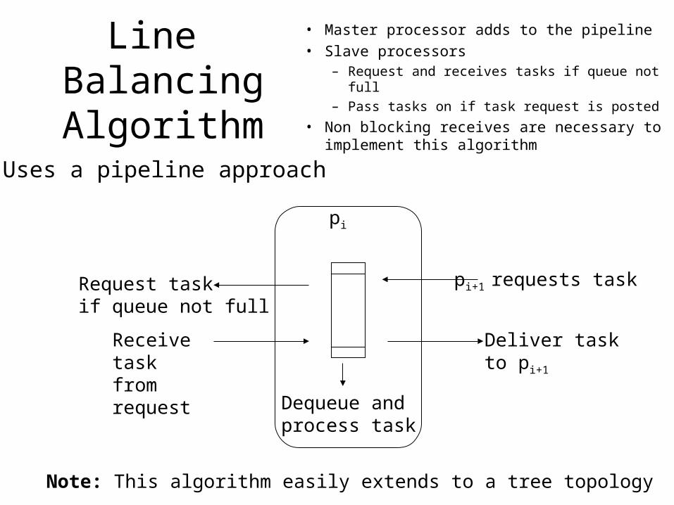
Line BalancingAlgorithm
• Master processor adds to the pipeline
• Slave processors– Request and receives tasks if queue not full
– Pass tasks on if task request is posted
• Non blocking receives are necessary to implement this algorithm
Uses a pipeline approach
Request taskif queue not full
Receive taskfrom request
Deliver task to pi+1
pi+1 requests task
Dequeue andprocess task
pi
Note: This algorithm easily extends to a tree topology

Semi-dynamic• Pseudo codeRun algorithmTime to check balance? Suspend application IF load is balanced, resume application Re-partition the load Distribute data structures among processors Resume execution
• Partitioning– Model application execution by a partitioning graph– Partitioning is an NP-Complete problem– Goals: Balance processing and minimize communication– Partitioning Heuristics
• Recursive Bisection, Simulated Annealing, Multi-level, MinEx– Data Redistribution
• Goal: Minimize the data movement cost

Partitioning Graph
P2R1
P5R3
P8R3
P4R1
P6R6
P2R1
P9R6
P4R4P7
R5
P1 P2
c4 c6
c2
c1
c7
c1c3
c8
c5c3
P1 Load = (9+4+7+2) + (4+3+1+7) = 37P2 Load = (6+2+4+8+5) + (4+3+1+7) = 40
Question: When can we move a task to improve load balance?

Distributed Termination
• Insufficient condition for distributed termination – Empty task queues at every process
• Sufficient condition for distributed termination requires– All local termination conditions satisfied– No messages in transit that could restart an inactive process
• Termination algorithms– Acknowledgment– Ring– Tree– Fixed energy distribution

Acknowledgement Termination
• Process Receives task– Immediately acknowledge if source is
not parent– Acknowledge parent as process goes
idle
• Process goes idle after it– completes processing local tasks– Sends all acknowledgments– Receives all acknowledgments
• Note– A process always becomes inactive
before its parent– The application can terminate when the
master goes idle
Active
Inactive
First task
Acknowledge first task
Pi
Pj
Definition: Parent is the process sending initial task to a process
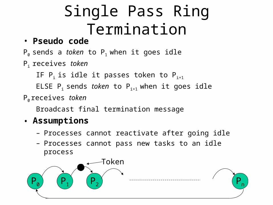
Single Pass Ring Termination• Pseudo codeP0 sends a token to P1 when it goes idle
Pi receives token
IF Pi is idle it passes token to Pi+1
ELSE Pi sends token to Pi+1 when it goes idle
P0 receives token
Broadcast final termination message
• Assumptions – Processes cannot reactivate after going idle
– Processes cannot pass new tasks to an idle process
P0 P1 P2 Pn
Token

Dual Pass Ring Termination
Pseudo code
WHEN P0 goes idle, it sends a white token to p1
WHEN Pi sends a task to Pj where j<i
Pi becomes a black process
WHEN Pi>0 receives token and goes idle
IF Pi is a black process
Pi colors the token black, Pi becomes White
ELSE Pi sends token to P(i+1)%n unchanged in color
IF P0 receives token and is idle IF token is White, application terminates
ELSE po sends a White token to P1
Handles task sent to a process that already passed the token onKey Point: Token and processors are colored either White or Black
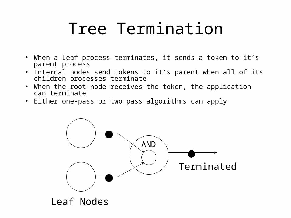
Tree Termination
• When a Leaf process terminates, it sends a token to it’s parent process• Internal nodes send tokens to it’s parent when all of its children
processes terminate• When the root node receives the token, the application can terminate• Either one-pass or two pass algorithms can apply
AND
Leaf Nodes
Terminated

Fixed Energy Termination
• P0 starts with full energy– When Pi receives a task, it also receives an energy allocation– When Pi spawns tasks, it assigns them to processors with
additional energy allocations within its allocation– When a process completes it returns its energy allotment
• The application terminates when the master becomes idle• Implementation
– Problem: Integer division eventually becomes zero– Solution:
o Use two level energy allocation <generation, energy>o The generation increases each time energy value goes to zero
Energy defined by an integer or long value

Example: Shortest Path Problem
DefinitionsGraph: Collection of nodes (vertices) and edgesDirected Graph: Edge can be traversed in only one directionWeighted Graph: Edges have weights that define costShortest Path Problem: Find the path from one node to another in a weighted graph that has the smallest accumulated weights
Applications1.Shortest distance between points on a map2.Quickest travel route3.Least expensive flight path4.Network routing5.Efficient manufacturing design

Climbing a Mountain
• Weights: expended effort• Directed graph
– Effort in one direction ≠ effort in another direction
– Ex: Downhill versus uphill
A B C D E F
A 10
B 8 13 24 51
C 14
D 9
E 17
F
A B C
DE
F
10 8132451
14
917
Adjacency Matrix
C 8
D 14 X
E 9 X
F 17 X
X
B 10 X
D 13
E 24
F 51
A
B
C
D
E
F Adjacency List
Graphic Representation

Moore’s Algorithm
• Assume – w[i][j] =weight of edge (i,j)– Dist[v] = distance to vertex v– Pred[v] = predecessor to vertex v
• Pseudo codeInsert the source vertex into a queueFor each vertex, v,
dist[v]=∞ infinity, dist[0] = 0WHILE (v = dequeue() exists) FOR (j=; j<n; j++) newdist = dist[i] + w[i][j] IF (newdist < dist[j]) dist[j] = newdist pred[j] = I append(j)
Less efficient than Dijkstra but more easily parallelized
i j
diwi,j
dj
dj=min(dj,di+wi,j)

Graph Analysis Stages
A 0 ∞ ∞ ∞ ∞ ∞
B 0 10 ∞ ∞ ∞ ∞
E
F E D C
D C
C E
0 10 18 23 34 61
0 10 18 23 34 51
0 10 18 23 32 51
0 10 18 23 32 51
0 10 18 23 32 49
A B C D E F
Vertex Queue Dist[j]
E D C 0 10 18 23 34 61

Centralized Work Pool Solution
• The Master maintains– The work pool queue of unchecked vertices– The distance array
• Every slave holds– The graph weights which is static
• The Slaves– Request a vertex– Compute new minimums– Send updated distance values and vertex to master
• The Master– Appends received vertices to its work queue– Sends new vertex and the updated distance array.

Distributed Work Pool Solution• Data held in each processor
– The graph weights– The distances to vertices stored locally– The processor assignments
• When a process receiving a distance:– If its local value is reduced
o Updates its local value of dist[v]o Send distances to adjacent vertices to appropriate processors
• Notes– Inefficient with one vertex per processor
o Poor computation to communication ratioo Many processors can be inactive
– One of the termination algorithms is necessary