Load Balancing for Partition-based Similarity Search

Xun Tang, Maha Alabduljalil, Xin Jin, Tao YangDepartment of Computer Science

University of California at Santa Barbara

SIGIR’14

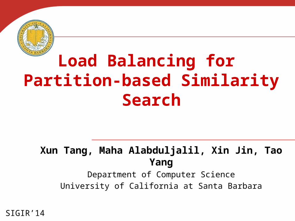
• Definition: Finding pairs of objects whose similarity is above a certain threshold

• Application examples: Document clustering

– Near duplicates– Spam detection

Query suggestions Advertisement fraud detection Collaborative filtering & recommendation

All Pairs Similarity Search (APSS)

≥ τSim (di,dj) = cos(di,dj)

di

dj

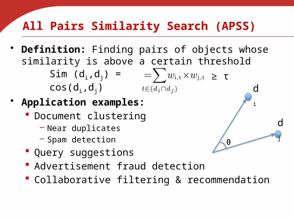
Big Data Challenges for Similarity Search

• 20M tweets fit in memory, but take days to process• Approximated processing

Df-limit [Lin SIGIR’09]: remove features with their vector frequency exceeding an upper limit

Sequential time (hour)

Values marked * are estimated by sampling

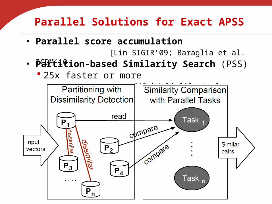
Parallel Solutions for Exact APSS

• Parallel score accumulation [Lin SIGIR’09; Baraglia et al.

ICDM’10

25x faster or more• Partition-based Similarity Search (PSS)

[Alabduljalil et al. WSDM’13]

Focus of This Paper

• Improves PSS by additional 41% By improving computation load balancing

Key techniques• Two-stage load assignment algorithm

First stage constructs a preliminary load assignment Second stage refines the assignment Analytical results on competitiveness to support

design• Improved dissimilarity detection with hierarchical

data partitioning

Previous Work

• Filtering Dynamic computation filtering. [Bayardo et al. WWW’07] Prefix, positional, and suffice filtering. [Xiao et al. WWW’08]

• Similarity-based grouping Inverted indexing. [Arasu et al. VLDB’06] Parallelization with MapReduce. [Lin SIGIR’09] Feature-sharing groups. [Vernica et al. SIGMOD’10] Locality-sensitive hashing. [Gionis et al. VLDB’99; Ture et al. SIGIR’11] Partition-based similarity comparison. [Alabduljalil et al. WSDM’13]

• Load balancing and scheduling Index serving in search systems. [Kayaaslan et al. TWEB’13] Division scheme with MapReduce. [Wang et al. KDD’13] Greedy scheduling policy. [Garey and Grahams. SIAM’75] Delay scheduling with Hadoop. [Zaharia et al. EuroSys’10]

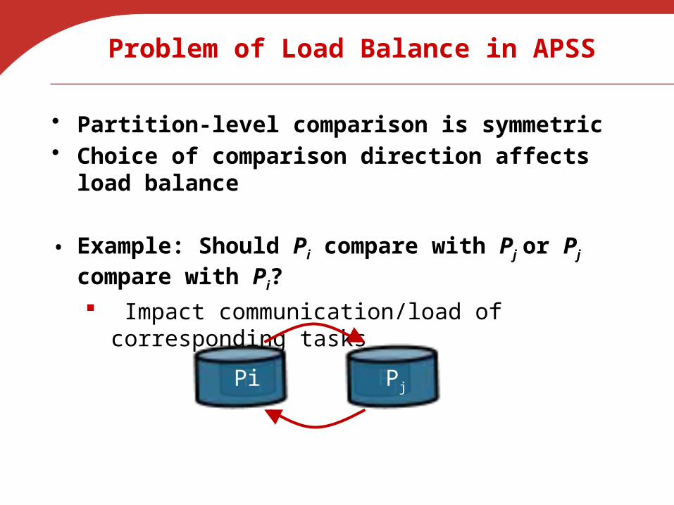
Problem of Load Balance in APSS

• Partition-level comparison is symmetric• Choice of comparison direction affects load balance

• Example: Should Pi compare with Pj or Pj compare with Pi?

Impact communication/load of corresponding tasks

Pi PjPjPi

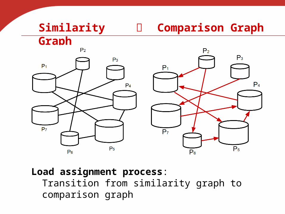
Similarity Graph Comparison Graph

Load assignment process:Transition from similarity graph to comparison graph

Load Balance Measurement & Examples

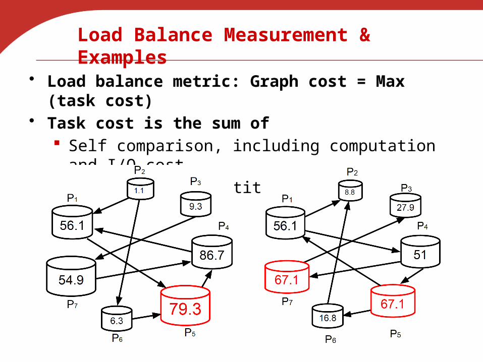
• Load balance metric: Graph cost = Max (task cost)• Task cost is the sum of

Self comparison, including computation and I/O cost Comparison to partitions point to itself

Challenges of Optimal Load Balance

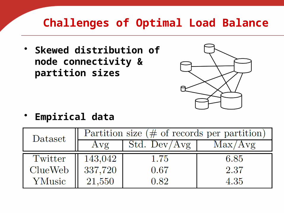
• Skewed distribution of node connectivity & partition sizes

• Empirical data

Two-Stage Load Balance

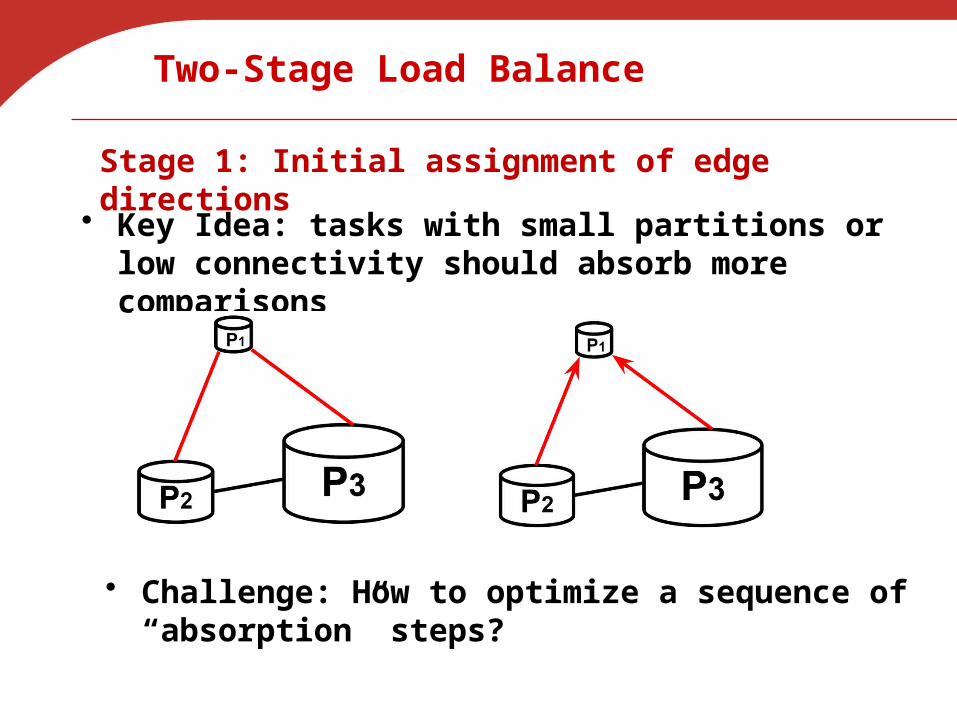
• Key Idea: tasks with small partitions or low connectivity should absorb more comparisons

Stage 1: Initial assignment of edge directions

• Challenge: How to optimize a sequence of “absorption” steps?

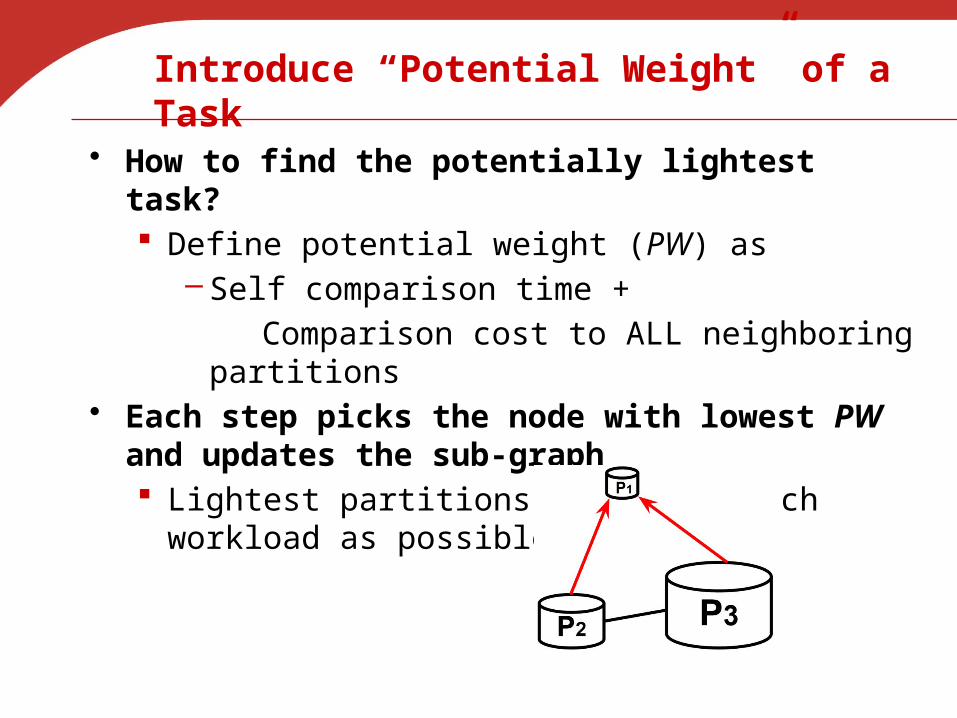
Introduce “Potential Weight” of a Task

• How to find the potentially lightest task? Define potential weight (PW) as

– Self comparison time +

Comparison cost to ALL neighboring partitions• Each step picks the node with lowest PW and

updates the sub-graph Lightest partitions absorb as much workload as

possible

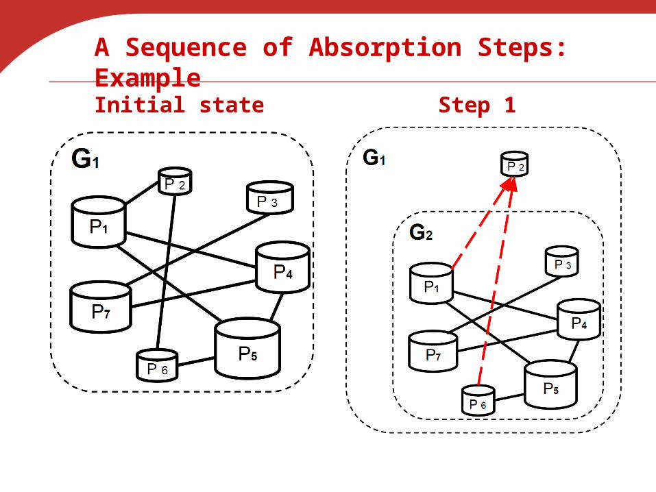
A Sequence of Absorption Steps: Example

Initial state Step 1

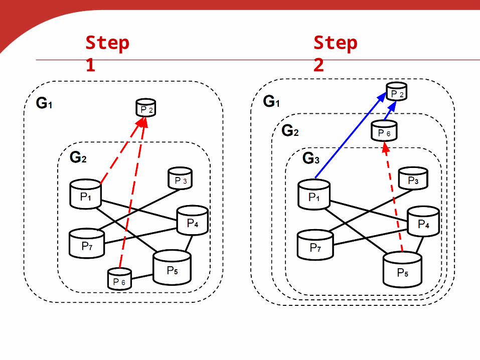
Step 2Step 1

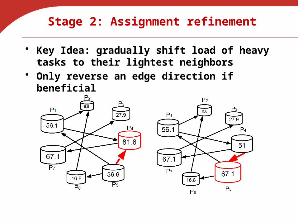
Stage 2: Assignment refinement

• Key Idea: gradually shift load of heavy tasks to their lightest neighbors

• Only reverse an edge direction if beneficial

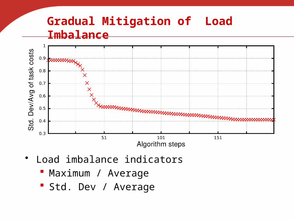
Gradual Mitigation of Load Imbalance

• Load imbalance indicators Maximum / Average Std. Dev / Average

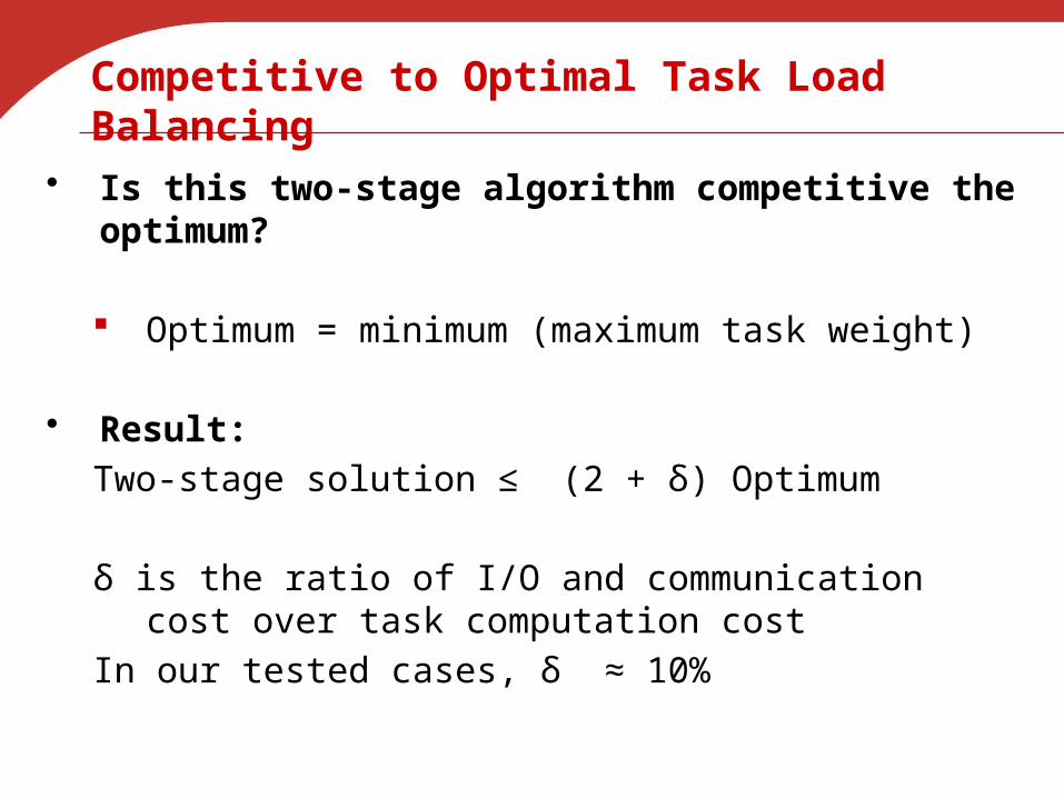
Competitive to Optimal Task Load Balancing

• Is this two-stage algorithm competitive the optimum?

Optimum = minimum (maximum task weight)

• Result:

Two-stage solution ≤ (2 + δ) Optimum

δ is the ratio of I/O and communication cost over task computation cost

In our tested cases, δ ≈ 10%

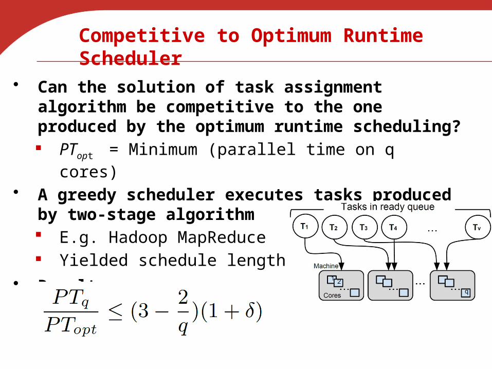
Competitive to Optimum Runtime Scheduler

• Can the solution of task assignment algorithm be competitive to the one produced by the optimum runtime scheduling? PTopt = Minimum (parallel time on q cores)

• A greedy scheduler executes tasks produced by two-stage algorithm E.g. Hadoop MapReduce Yielded schedule length is PTq

• Result:

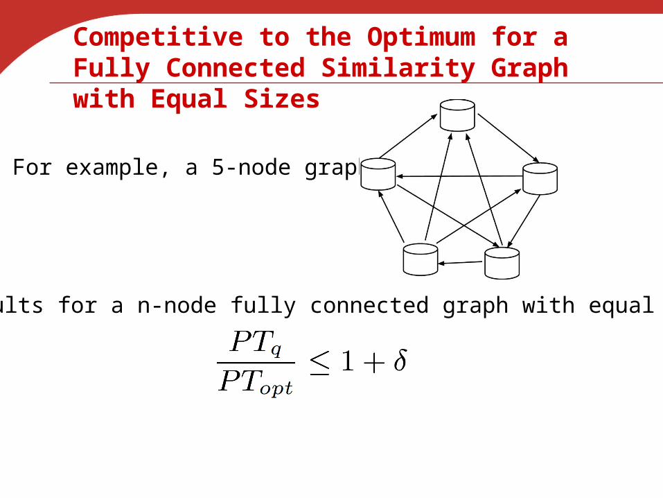
Competitive to the Optimum for a Fully Connected Similarity Graph with Equal Sizes

For example, a 5-node graph

Results for a n-node fully connected graph with equal sizes

Evaluations

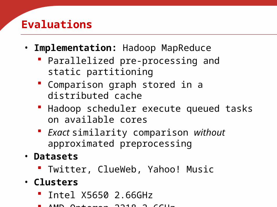
• Implementation: Hadoop MapReduce Parallelized pre-processing and static partitioning Comparison graph stored in a distributed cache Hadoop scheduler execute queued tasks on

available cores Exact similarity comparison without approximated

preprocessing• Datasets

Twitter, ClueWeb, Yahoo! Music• Clusters

Intel X5650 2.66GHz AMD Opteron 2218 2.6GHz

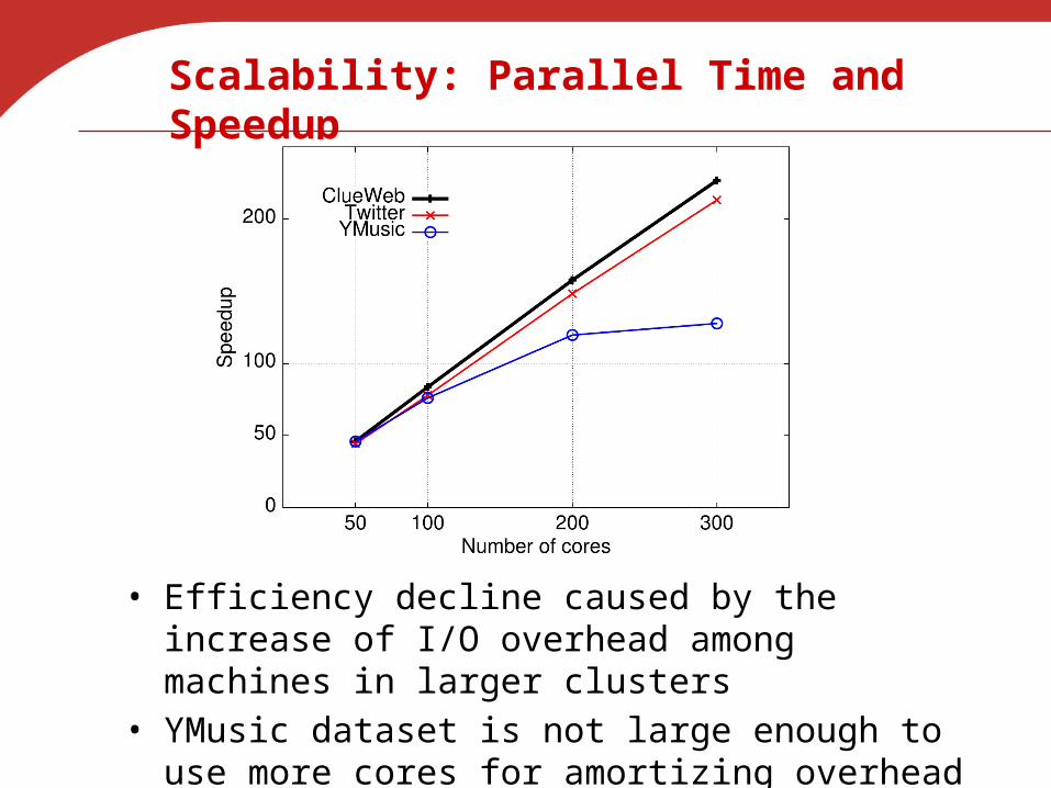
Scalability: Parallel Time and Speedup

• Efficiency decline caused by the increase of I/O overhead among machines in larger clusters

• YMusic dataset is not large enough to use more cores for amortizing overhead

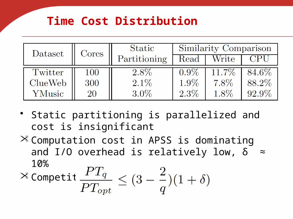
Time Cost Distribution

• Static partitioning is parallelized and cost is insignificant• Computation cost in APSS is dominating and I/O

overhead is relatively low, δ ≈ 10%• Competitive to optimum rumtime

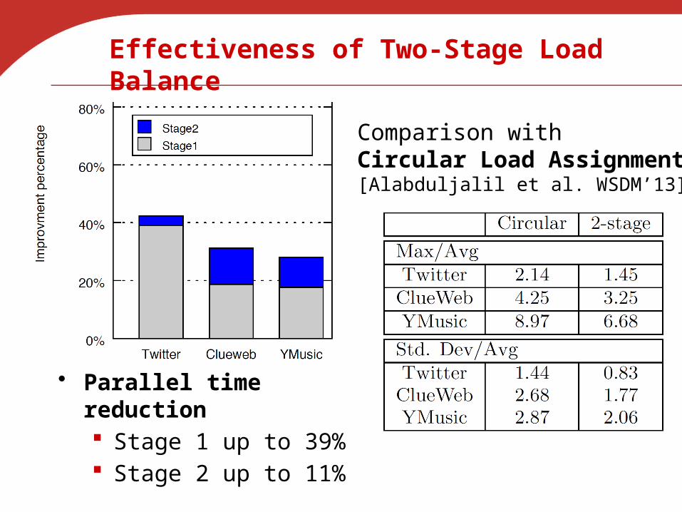
Effectiveness of Two-Stage Load Balance

Comparison withCircular Load Assignment [Alabduljalil et al. WSDM’13]

• Parallel time reduction Stage 1 up to 39% Stage 2 up to 11%

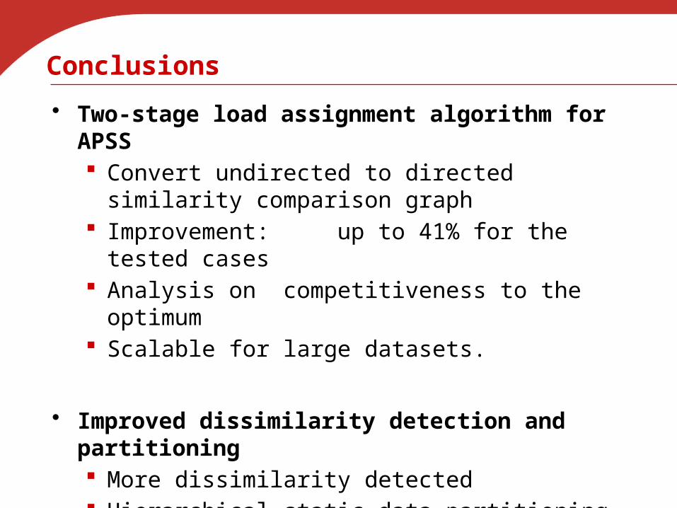
Conclusions

• Two-stage load assignment algorithm for APSS Convert undirected to directed similarity

comparison graph Improvement: up to 41% for the tested cases Analysis on competitiveness to the optimum Scalable for large datasets.

• Improved dissimilarity detection and partitioning More dissimilarity detected Hierarchical static data partitioning method for more

even sizes Contributes up to 18% end-performance gain

Q & A

Thank you!

Presenter: Xun Tangxtang@cs.ucsb.eduLook for challenging opportunities.

Backup Slides

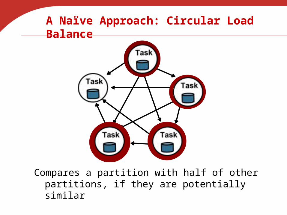
A Naïve Approach: Circular Load Balance

Compares a partition with half of other partitions, if they are potentially similar

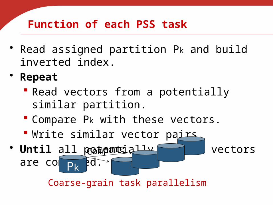
Function of each PSS task

• Read assigned partition Pk and build inverted index.• Repeat

Read vectors from a potentially similar partition. Compare Pk with these vectors. Write similar vector pairs.

• Until all potentially similar vectors are compared.

Compare

Coarse-grain task parallelism

Pk

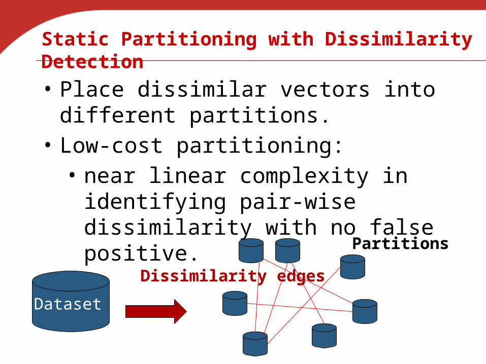
Static Partitioning with Dissimilarity Detection

• Place dissimilar vectors into different partitions.

• Low-cost partitioning: • near linear complexity in identifying pair-

wise dissimilarity with no false positive.

Dataset

Partitions

Dissimilarity edges

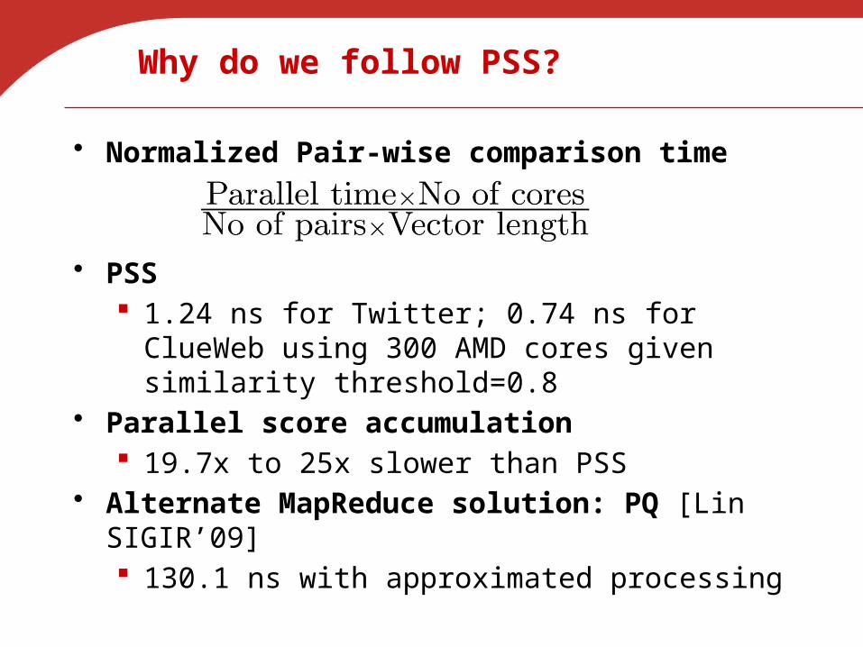
Why do we follow PSS?

• Normalized Pair-wise comparison time

• PSS 1.24 ns for Twitter; 0.74 ns for ClueWeb using 300

AMD cores given similarity threshold=0.8• Parallel score accumulation

19.7x to 25x slower than PSS• Alternate MapReduce solution: PQ [Lin SIGIR’09]

130.1 ns with approximated processing

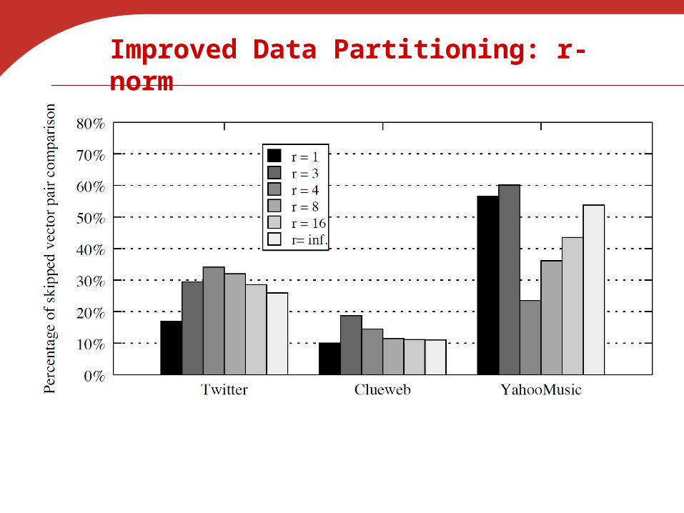
Improved Data Partitioning: r-norm

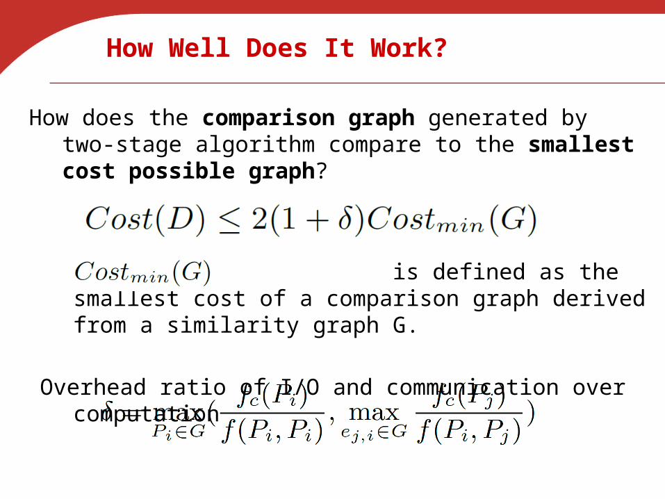
How Well Does It Work?

How does the comparison graph generated by two-stage algorithm compare to the smallest cost possible graph?

is defined as the smallest cost of a comparison graph derived from a similarity graph G.

Overhead ratio of I/O and communication over computation

How Well Does It Work?

How is our job completion time compare to the optimal solution? Not knowing the allocated computing resources.

is the job completion time of the two-stage load assignment with a greedy scheduler on q cores; is that of an optimal solution.

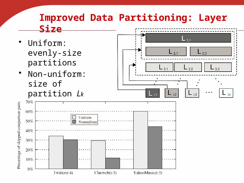
Improved Data Partitioning: Layer Size

• Uniform: evenly-size partitions

• Non-uniform:size of partition Lk proportional to index k

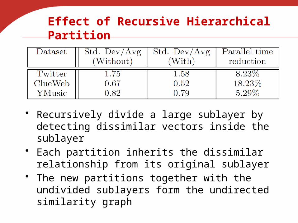
Effect of Recursive Hierarchical Partition

• Recursively divide a large sublayer by detecting dissimilar vectors inside the sublayer

• Each partition inherits the dissimilar relationship from its original sublayer

• The new partitions together with the undivided sublayers form the undirected similarity graph