G. Bebis et al. (Eds.): ISVC 2014, Part I, LNCS 8887, pp. 579–588, 2014. © Springer International Publishing Switzerland 2014

Automatic Multi-light White Balance Using Illumination Gradients and Color Space Projection

Clifford Lindsay and Emmanuel Agu

Worcester Polytechnic Institute, Worcester, MA

Abstract. White balance algorithms try to remove color casts in images caused by non-white scene illuminants, transforming the images to appear as if they were taken under a canonical light source. We propose a new white balance al-gorithm for scenes with multiple lights, which requires that the colors of all scene illuminants and their relative contributions to each image pixel are deter-mined. Prior work on multi-illuminant white balance either required user input or made restrictive assumptions. We identify light colors as areas of maximum gradients in the indirect lighting component. The colors of each maximal point are clustered in RGB space in order to estimate the distinct global light colors. Once the light colors are determined, we project each image pixel in RGB space to determine the relative contribution of each distinct light color to each image pixel. Our white balance method for images with multiple light sources is fully automated and amenable to hardware implementation.

1 Introduction

Color constancy is the ability of the Human Visual System (HVS) to mitigate the effects of different lights on a scene such that the perceived color of scene objects is unchanged under different illumination [19]. For example, using color constancy, the HVS removes the unnatural yellow tint that results from incandescent lighting or a blue cast caused by the early morning sun. In photography, the process of color con-stancy is mimicked by applying a white balance method to a photograph after capture in order to remove colors cast by non-canonical lighting. White balance is a crucial processing step in the photographic pipeline [14].

Most prior work on white balance methods make the simplifying assumption that the entire photographed scene is illuminated by a single light source. However, most real-world scenes contain multiple lights and the illumination recorded at each camera pixel includes the combined influence of these light sources. White balancing images taken with multiple light sources involves estimating the color and intensity of each contributing light source from a single image, which is a challenging, ill-posed prob-lem. Consequently, most of today’s cameras and photo-editing software employ white balance techniques that make classic (simpler) assumptions, such as the Grey World assumption [3], which assumes the scene being white balanced contains only a single light source. To white balance multi-illuminant scenes, some techniques segment the image and then white balance each region separately using traditional single-light techniques. However, this approach can result in hard transitions in white balanced

580 C. Lindsay and E. Agu

images as neighboring regions can estimate different light sources at region bounda-ries and does not account for partial lighting contributions from light sources.

We propose a technique to white balance images that contain two different colored light sources by estimating the color of each light and determining their appropriate contribution to each camera pixel. Our white balance technique has two main steps. First, we separate the input scene into direct and indirect lighting components and determine each light color by using global illumination gradients in the indirect light-ing component to determine local maxima. We then use a projection in RGB space to determine the relative contribution of each light source to each pixel’s color. Since it uses mostly vector math, our technique is amenable to on-camera hardware imple-mentation and real-time executions.

Our Main Contributions: 1) A fully automated two-light white balance method re-quiring no user interaction. 2) A gradient-based method for determining the color of each light source. 3) A projection method in RGB color space to determine the rela-tive influence of each light source on a given pixel. 4) A hardware implementation amenable to real time execution on commodity cameras.

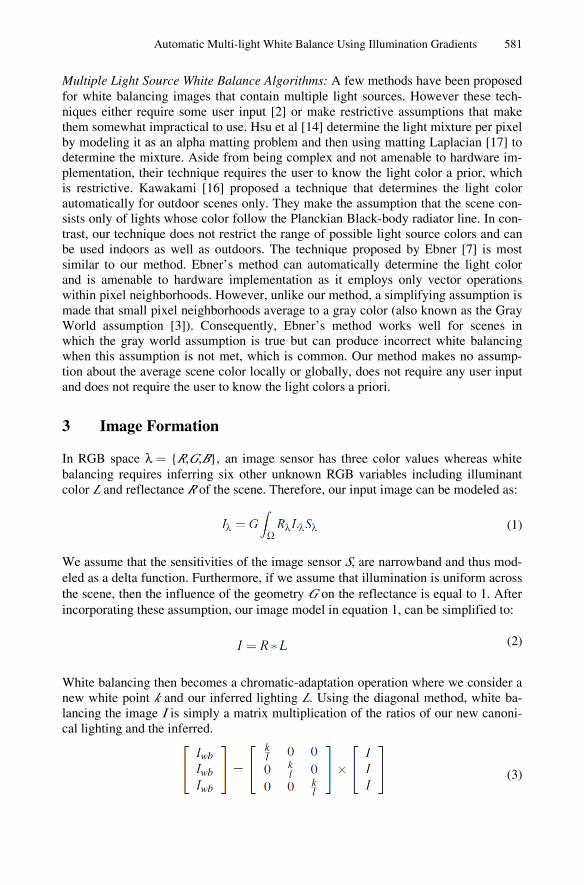
Fig. 1. Left is original image of a scene with multiple lights, center image is white-balanced using our method, and right is white balanced using Ebner’s method [7]

2 Related Work

Single Light Source White Balance Algorithms: Research into solving the color con-stancy and white balance problems has yielded many techniques for single light source white balance. Classical color constancy techniques based on simple statistical methods include the Gray World [3] and Max RGB [18] algorithms. These techniques make simplifying assumptions about scene or image statistics (e.g. Gray world as-sumes scene reflectance average to gray), which work only in special cases but fail in more general application. Higher order statistical methods such as Generalized Grey World [12], the Grey-Edge algorithm [21], and techniques employing natural image statistics [13] have successfully solved illumination estimation problems. Other pro-posed approaches apply Bayesian statistics to estimate scene illumination [10], make assumptions about the color spaces such as Gamut Mapping [9] or color shifts [8], or using machine learning techniques such as Neural Networks [4]. The majority of the color constancy and white balance research, including the methods just mentioned, assume that the scene is illuminated by a single light source.

Automatic Multi-light White Balance Using Illumination Gradients 581

Multiple Light Source White Balance Algorithms: A few methods have been proposed for white balancing images that contain multiple light sources. However these tech-niques either require some user input [2] or make restrictive assumptions that make them somewhat impractical to use. Hsu et al [14] determine the light mixture per pixel by modeling it as an alpha matting problem and then using matting Laplacian [17] to determine the mixture. Aside from being complex and not amenable to hardware im-plementation, their technique requires the user to know the light color a prior, which is restrictive. Kawakami [16] proposed a technique that determines the light color automatically for outdoor scenes only. They make the assumption that the scene con-sists only of lights whose color follow the Planckian Black-body radiator line. In con-trast, our technique does not restrict the range of possible light source colors and can be used indoors as well as outdoors. The technique proposed by Ebner [7] is most similar to our method. EbnerÊs method can automatically determine the light color and is amenable to hardware implementation as it employs only vector operations within pixel neighborhoods. However, unlike our method, a simplifying assumption is made that small pixel neighborhoods average to a gray color (also known as the Gray World assumption [3]). Consequently, EbnerÊs method works well for scenes in which the gray world assumption is true but can produce incorrect white balancing when this assumption is not met, which is common. Our method makes no assump-tion about the average scene color locally or globally, does not require any user input and does not require the user to know the light colors a priori.

3 Image Formation

In RGB space λ = {R,G,B}, an image sensor has three color values whereas white balancing requires inferring six other unknown RGB variables including illuminant color L and reflectance R of the scene. Therefore, our input image can be modeled as:

(1)

We assume that the sensitivities of the image sensor S, are narrowband and thus mod-eled as a delta function. Furthermore, if we assume that illumination is uniform across the scene, then the influence of the geometry G on the reflectance is equal to 1. After incorporating these assumption, our image model in equation 1, can be simplified to:

(2)

White balancing then becomes a chromatic-adaptation operation where we consider a new white point k and our inferred lighting L. Using the diagonal method, white ba-lancing the image I is simply a matrix multiplication of the ratios of our new canoni-cal lighting and the inferred.

(3)

582 C. Lindsay and E. Agu

3.1 Multiple Illuminants

Color constancy and white balance algorithms generally fall into two broad catego-ries; 1) Techniques that determine the reflectance of objects within the scene and 2) Techniques that transform an input image in order to discount the effects of non-canonical scene lighting. Our method falls within the latter category. Consequently, we are not concerned with recovering reflectance but instead in determining unknown illuminants and discounting their effects. If we assume that the scene is illuminated by two unknown illuminants with different colors, we can assume that each pixel, lo-cated at (x,y) in image I, has a relative contribution of light from each illuminant in the form:

(4)

Assuming the light contributions from L1 and L2 are conserved, then 0 < α < 1, and all light present in the scene comes from only these lights (i.e. no florescence). I(x,y) is a result of the reflectance within the scene scaled by some factor G. The task of white balancing image I then becomes one of first a) determining the colors of L1 and L2 in RGB space and then b) determining their relative contributions, α to pixel I(x,y).

4 Our Method

4.1 Determining the Illuminant Color Using a Gradient Domain Technique

Ruppertsberg and Bloj [22] suggest that the ability of the human visual system to provide a robust mechanism for color constancy is anchored in its ability to discern indirect lighting. Indirect lighting causes smaller appearance changes than the combi-nation of direct and indirect lighting. Based on these findings, we use indirect lighting as the primary input for our light color estimation method after decomposing the scene into its direct and indirect components. Decomposition of direct and indirect lighting is possible using the method proposed by Nayar et al. [20]. The indirect com-ponent is then used to determine reference points within the scene that provides the best estimate of the light color. Using the gradient magnitude of the luminance, we can determine areas of the scene with high concentrations of photons (local maxima in the gradient domain) to use as reference points.

For estimating light color, we incorporate KajiyaÊs Rendering equation [15]. If we assume that incident radiance is integrated over a hemisphere and that a single light source is present (no light emitting surfaces), then the reflectance from our image model in equation 5 can be expanded to include global effects as described by the Rendering equation. Equation 6 is our image formation model based on the global (indirect) component of the scene only. Since the continuous form of the integral in equation 6 is difficult to evaluate, we discretize the integral (equation 7).

(5)

(6)

Automatic Multi-light White Balance Using Illumination Gradients 583

(7)

The hemisphere is sampled using a cosine weighted sampling method in N directions as described in [5], allowing the PDF= cos(θ)/π. to be evaluated. This simplifies the equation and yields a simplified approximate solution for the value of the lighting L.

(8)

Because (1/ πR) is an unknown scaling factor, R cannot be assumed to be a constant. For L to be constant throughout the scene, we devise a method for selecting the ap-propriate location for which we can estimate L. We do this using a gradient-based technique on the indirect lighting component. In particular, we find local maxima within the scene’s gradient field using a divergence operator, which measures the gradient fieldÊs tendency toward a sink (negative divergence) or source (positive di-vergence). Since we are only interested in areas in which photons collect, we consider only areas of negative divergence, which we call light sinks.

(9)

In equation 9, the gradient field F is defined over the dimensions of the image (x,y). The divergence of gradient field F is then defined over the partial derivative of the x direction δU and the y direction δV with respect to partial derivatives of the x and y direction. The light sink then has a maximum divergence when the ∇· F has a maxi-mum negative value. Since we assume that each light will produce at least one light sink, these values can be clustered in the RGB cube to estimate the light colors.

4.2 Determining the Illuminant Contributions Using Color Space Projection

In this section our method for determining the relative contributions of each light source for each pixel in the image (solving for α), is described. This is accomplished by using geometric interpretations of the relationship between the light colors and the image pixel which exhibits unknown reflectance. A linear RGB color space is as-sumed and no Gamma correction is needed or has already been applied.

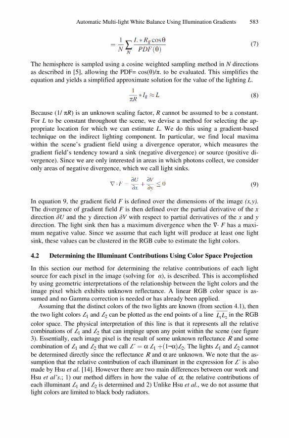
Assuming that the distinct colors of the two lights are known (from section 4.1), then the two light colors L1 and L2 can be plotted as the end points of a line

21LL in the RGB

color space. The physical interpretation of this line is that it represents all the relative combinations of L1 and L2 that can impinge upon any point within the scene (see figure 3). Essentially, each image pixel is the result of some unknown reflectance R and some combination of L1 and L2 that we call L´ = α L1 +(1−α)L2. The lights L1 and L2 cannot be determined directly since the reflectance R and α are unknown. We note that the as-sumption that the relative contribution of each illuminant in the expression for L´ is also made by Hsu et al. [14]. However there are two main differences between our work and Hsu et al’s.; 1) our method differs in how the value of α, the relative contributions of each illuminant L1 and L2 is determined and 2) Unlike Hsu et al., we do not assume that light colors are limited to black body radiators.

584 C. Lindsay and E. Agu

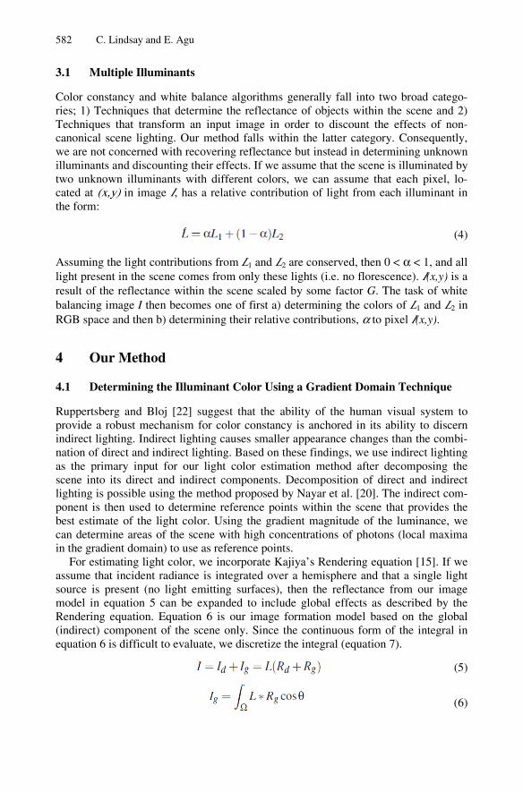
Fig. 2. Images showing the divergence operations used to indentify sink locations. Top left is the original image. Top right is the indirect image used to calculated the gradient and diver-gence of the image. Bottom left, is the gradient field overlayed on the original image. Bottom right is a heatmap that indicates the level of divergence, where red is 0 divergence and blue is maximum negative divergence. The green arrows show the light sinks.

We solve this ill-posed problem and determine L´ by assuming that small pixel neighborhoods N can be modeled by the color line model [17]. A small group of pix-els in the same region are highly coherent in terms of their color and follow the color line model. If we assume that the illumination is constant in this small region, then the variation in color of each pixel is caused by changes in the reflectance. If we extend this color line out infinitely, then we can estimate the L´ as the point on

21LL that is

closest to the line LN formed by the neighborhood of pixels N (this is represented by a dashed line in figure 3). This translates the problem from determing an unknown ref-lectance and light contribution into solving for the minimal value of v, which is the line with the shortest distance connecting LN and

21LL expressed as:

(10)

Fig. 3. The relationship between a pixel I(x,y) in the image at (x,y) and the contributions of two lights in linear RGB space. The two light sources L1 and L2 form a line and each image pixel is illuminated by some linear interpolation of L1 and L2 denoted α, located on that line.

Automatic Multi-light White Balance Using Illumination Gradients 585

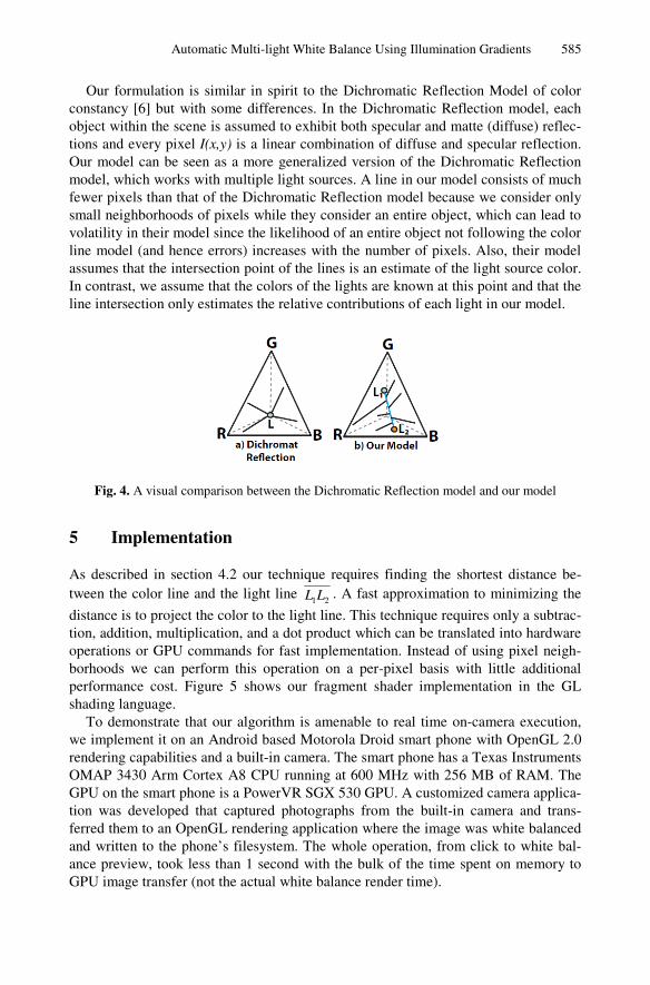
Our formulation is similar in spirit to the Dichromatic Reflection Model of color constancy [6] but with some differences. In the Dichromatic Reflection model, each object within the scene is assumed to exhibit both specular and matte (diffuse) reflec-tions and every pixel I(x,y) is a linear combination of diffuse and specular reflection. Our model can be seen as a more generalized version of the Dichromatic Reflection model, which works with multiple light sources. A line in our model consists of much fewer pixels than that of the Dichromatic Reflection model because we consider only small neighborhoods of pixels while they consider an entire object, which can lead to volatility in their model since the likelihood of an entire object not following the color line model (and hence errors) increases with the number of pixels. Also, their model assumes that the intersection point of the lines is an estimate of the light source color. In contrast, we assume that the colors of the lights are known at this point and that the line intersection only estimates the relative contributions of each light in our model.

Fig. 4. A visual comparison between the Dichromatic Reflection model and our model

5 Implementation

As described in section 4.2 our technique requires finding the shortest distance be-tween the color line and the light line

21LL . A fast approximation to minimizing the

distance is to project the color to the light line. This technique requires only a subtrac-tion, addition, multiplication, and a dot product which can be translated into hardware operations or GPU commands for fast implementation. Instead of using pixel neigh-borhoods we can perform this operation on a per-pixel basis with little additional performance cost. Figure 5 shows our fragment shader implementation in the GL shading language.

To demonstrate that our algorithm is amenable to real time on-camera execution, we implement it on an Android based Motorola Droid smart phone with OpenGL 2.0 rendering capabilities and a built-in camera. The smart phone has a Texas Instruments OMAP 3430 Arm Cortex A8 CPU running at 600 MHz with 256 MB of RAM. The GPU on the smart phone is a PowerVR SGX 530 GPU. A customized camera applica-tion was developed that captured photographs from the built-in camera and trans-ferred them to an OpenGL rendering application where the image was white balanced and written to the phone’s filesystem. The whole operation, from click to white bal-ance preview, took less than 1 second with the bulk of the time spent on memory to GPU image transfer (not the actual white balance render time).

586 C. Lindsay and E. Agu

Fig. 5. GLSL pixel shader code projects a pixel to the light line then white balances the pixel

6 Results

We compared our white balanced images with the ground truth and with other me-thods. Our test scenes comprise synthetic images with known illuminant colors. The synthetic images were rendered in a physically based renderer that produced physical-ly accurate direct and indirect lighting (global illumination). Every effort was made to use plausible light source colors in order to test the performance of our white balance algorithms on real-world illumination. Unlike prior white balance algorithms which assume that the colors of the illuminants lie close to the Planckian Locus of the CIE chart [11], we assume that light source colors lie within the boundary of the sRGB gamut. In addition to expanding the colors of the light sources, we also produce good results with low-light images and with scenes that exhibit low-color complexity, on which white balance algorithms generally perform poorly [1].

Our method works well when there is enough indirect lighting to perform a separa-tion into direct and indirect lighting and that there are at least two light sinks. A fail-ure results when there is an incorrect sink calculation or there is simply no light sink for one or two of the light sources. Though we have found that light sinks are com-mon in most scenes, there is a need on occasion to hand tune the size of the gradient magnitudes in order to accurately distinguish the light sink from other features and noise within the scene. It is also assumed that the values of the pixels within the im-age are not saturated pixels resulting in clamped values.

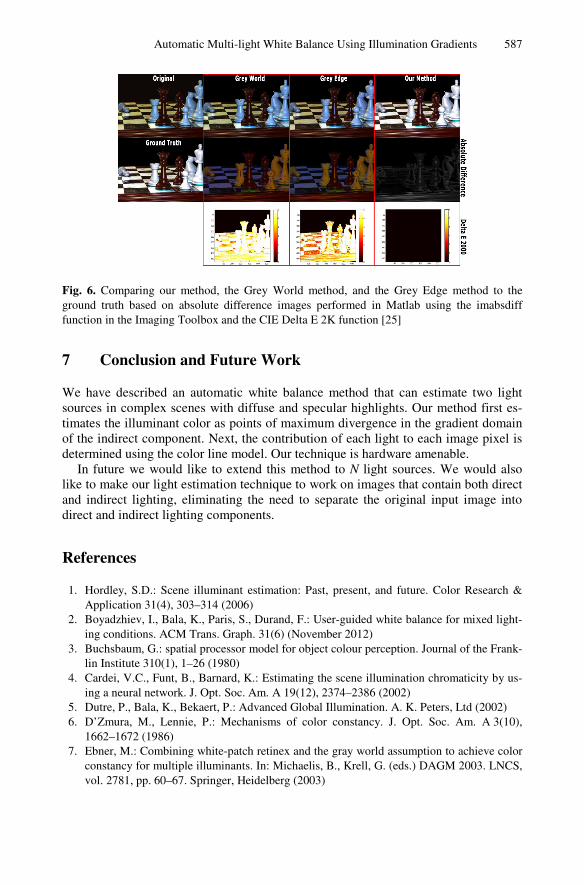
In the presence of both specular and diffuse reflection our light contribution me-thod works well as can be seen from figure 6. The chess scene has many specular highlights as well as diffuse reflection. The light colors in the chess scene are visually quite different and is similar to what might occur during flash photograph under in-candescent lighting. The foreground is lit by a cool blue light from the flash whereas the background is lit by a reddish-yellow artificial light. This contrast in light color shows how robust our method is to colors outside the group of black body radiators, which is not possible with previous white balance algorithms. As the differences be-tween the two lights increase, the error associated with traditional single light source white balance methods grows. This results in errors noticeable in the absolute differ-ence images. In figure 6 we show the chess scene again with comparisons with the traditional gray world [3] and the gray edge methods [23].

Automatic Multi-light White Balance Using Illumination Gradients 587

Fig. 6. Comparing our method, the Grey World method, and the Grey Edge method to the ground truth based on absolute difference images performed in Matlab using the imabsdiff function in the Imaging Toolbox and the CIE Delta E 2K function [25]

7 Conclusion and Future Work

We have described an automatic white balance method that can estimate two light sources in complex scenes with diffuse and specular highlights. Our method first es-timates the illuminant color as points of maximum divergence in the gradient domain of the indirect component. Next, the contribution of each light to each image pixel is determined using the color line model. Our technique is hardware amenable.

In future we would like to extend this method to N light sources. We would also like to make our light estimation technique to work on images that contain both direct and indirect lighting, eliminating the need to separate the original input image into direct and indirect lighting components.

References

1. Hordley, S.D.: Scene illuminant estimation: Past, present, and future. Color Research & Application 31(4), 303–314 (2006)

2. Boyadzhiev, I., Bala, K., Paris, S., Durand, F.: User-guided white balance for mixed light-ing conditions. ACM Trans. Graph. 31(6) (November 2012)

3. Buchsbaum, G.: spatial processor model for object colour perception. Journal of the Frank-lin Institute 310(1), 1–26 (1980)

4. Cardei, V.C., Funt, B., Barnard, K.: Estimating the scene illumination chromaticity by us-ing a neural network. J. Opt. Soc. Am. A 19(12), 2374–2386 (2002)

5. Dutre, P., Bala, K., Bekaert, P.: Advanced Global Illumination. A. K. Peters, Ltd (2002) 6. D’Zmura, M., Lennie, P.: Mechanisms of color constancy. J. Opt. Soc. Am. A 3(10),

1662–1672 (1986) 7. Ebner, M.: Combining white-patch retinex and the gray world assumption to achieve color

constancy for multiple illuminants. In: Michaelis, B., Krell, G. (eds.) DAGM 2003. LNCS, vol. 2781, pp. 60–67. Springer, Heidelberg (2003)

588 C. Lindsay and E. Agu

8. Ebner, M.: Color constancy using local color shifts. In: Pajdla, T., Matas, J(G.) (eds.) ECCV 2004. LNCS, vol. 3023, pp. 276–287. Springer, Heidelberg (2004)

9. Finlayson, G.D., Hordley, S.D.: Improving gamut mapping color constancy. IEEE Trans-actions Image Processing 9, 1774–1783 (2000)

10. Finlayson, G.D., Hordley, S., Hubel, P.M.: Color by correlation: A simple, unifying frame-work for color constancy. IEEE Trans. Pattern Anal. Mach. Intell. 23(11), 1209–1221 (2001)

11. Luo, M.R., Cui, G., Rigg, B.: The development of the cie 2000 colour-difference fomula: Ciede2000. Color Research & Application 26(5), 340–350 (2001)

12. Finlayson, G.D., Trezzi, E.: Shades of gray and colour constancy. In: Color Imaging Con-ference (2004)

13. Gijsenij, A., Gevers, T.: Color constancy using natural image statistics. In: IEEE Computer Society Conference on Computer Vision and Pattern Recognition, pp. 1–8 (2007)

14. Hsu, E., Mertens, T., Paris, S., Avidan, S., Durand, F.: Light mixture estimation for spa-tially varying white balance. In: SIGGRAPH 2008, pp. 1–7 (2008)

15. Kajiya, J.T.: The rendering equation. In: ACM SIGGRAPH 1986, pp. 143–150 (1986) 16. Kawakami, R., Ikeuchi, K., Tan, R.T.: Consistent surface color for texturing large objects

in outdoor scenes. In: Proc ICCV 2005, pp. 1200–1207 (2005) 17. Levin, A., Lischinski, D., Weiss, Y.: A closed form solution to natural image matting. In:

Proc CVPR 2006, pp. 61–68 (2006) 18. Land, E.H., McCann, J.J.: Lightness and retinex theory. J. Opt. Soc. Am. 61(1), 1–11

(1971) 19. Wandell, B.A.: Foundations of Vision, Sinauer Associates, Sunderland MA (1995) 20. Nayar, S.K., Krishnan, G., Grossberg, M.D., Raskar, R.: Fast separation of direct and

global components of a scene using high frequency illumination. In: Proc ACM SIGGRAPH 2006, pp. 935–944 (2006)

21. Van De Weijer, J., Gevers, T., Gijsenij, A.: Edge-based color constancy. IEEE Transac-tions on Image Processing 16(9), 2207–2214 (2007)

22. Ruppertsberg, A.I., Bloj, M.: Reflecting on a room of one reflectance. J. Vis. 7(13), 1–13 (2007)