Embed Size (px)
Citation preview
Timed Automata: Semantics, Algorithms and Tools
Johan Bengtsson and Wang Yi�
Uppsala University{johanb,yi}@it.uu.se
Abstract. This chapter is to provide a tutorial and pointers to results and relatedwork on timed automata with a focus on semantical and algorithmic aspects ofverification tools. We present the concrete and abstract semantics of timed au-tomata (based on transition rules, regions and zones), decision problems, andalgorithms for verification. A detailed description on DBM (Difference BoundMatrices) is included, which is the central data structure behind several verifica-tion tools for timed systems. As an example, we give a brief introduction to thetool UPPAAL.
1 Introduction
Timed automata is a theory for modeling and verification of real time systems. Exam-ples of other formalisms with the same purpose, are timed Petri Nets, timed processalgebras, and real time logics [17, 42, 47, 40, 8, 20]. Following the work of Alur andDill [5, 6], several model checkers have been developed with timed automata being thecore of their input languages e.g. [50, 33]. It is fair to say that they have been the driv-ing force for the application and development of the theory. The goal of this chapter isto provide a tutorial on timed automata with a focus on the semantics and algorithmsbased on which these tools are developed.
In the original theory of timed automata [5, 6], a timed automaton is a finite-stateBüchi automaton extended with a set of real-valued variables modeling clocks. Con-straints on the clock variables are used to restrict the behavior of an automaton, andBüchi accepting conditions are used to enforce progress properties. A simplified ver-sion, namely Timed Safety Automata is introduced in [28] to specify progress propertiesusing local invariant conditions. Due to its simplicity, Timed Safety Automata has beenadopted in several verification tools for timed automata e.g. UPPAAL [33] and Kronos[50]. In this presentation, we shall focus on Timed Safety Automata, and following theliterature, refer them as Timed Automata or simply automata when it is understood fromthe context.
The rest of the chapter is organized as follows: In the next section, we describe thesyntax and operational semantics of timed automata. The section also addresses deci-sion problems relevant to automatic verification. In the literature, the decidability andundecidability of such problems are often considered to be the fundamental proper-ties of a computation model. Section 3 presents the abstract version of the operational
� Corresponding author: Wang Yi, Division of Computer Systems, Department of InformationTechnology, Uppsala University, Box 337, 751 05 Uppsala, Sweden. Email: [email protected]
J. Desel, W. Reisig, and G. Rozenberg (Eds.): ACPN 2003, LNCS 3098, pp. 87–124, 2004.c© Springer-Verlag Berlin Heidelberg 2004
88 Johan Bengtsson and Wang Yi
semantics based on regions and zones. Section 4 describes the data structure DBM (Dif-ference Bound Matrices) for the efficient representation and manipulation of zones, andoperations on zones, needed for symbolic verification. Section 5 gives a brief introduc-tion to the verification tool UPPAAL. Finally, as an appendix, we list the pseudo-codefor the presented DBM algorithms.
2 Timed Automata
A timed automaton is essentially a finite automaton (that is a graph containing a finiteset of nodes or locations and a finite set of labeled edges) extended with real-valuedvariables. Such an automaton may be considered as an abstract model of a timed sys-tem. The variables model the logical clocks in the system, that are initialized with zerowhen the system is started, and then increase synchronously with the same rate. Clockconstraints i.e. guards on edges are used to restrict the behavior of the automaton. Atransition represented by an edge can be taken when the clocks values satisfy the guardlabeled on the edge. Clocks may be reset to zero when a transition is taken.
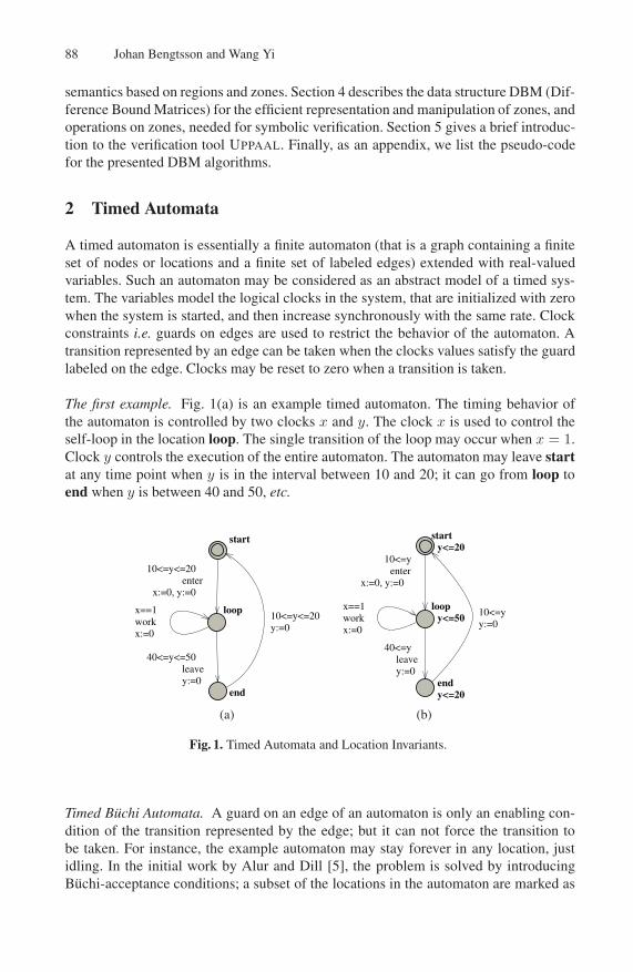
The first example. Fig. 1(a) is an example timed automaton. The timing behavior ofthe automaton is controlled by two clocks x and y. The clock x is used to control theself-loop in the location loop. The single transition of the loop may occur when x = 1.Clock y controls the execution of the entire automaton. The automaton may leave startat any time point when y is in the interval between 10 and 20; it can go from loop toend when y is between 40 and 50, etc.
start
loop
end
x:=0, y:=0
10<=y<=20enter
40<=y<=50
y:=0leave
x==1
x:=0work
10<=y<=20y:=0
starty<=20
loopy<=50
endy<=20
x:=0, y:=0
10<=yenter
40<=y
y:=0leave
x==1
x:=0work
10<=yy:=0
(a) (b)
Fig. 1. Timed Automata and Location Invariants.
Timed Büchi Automata. A guard on an edge of an automaton is only an enabling con-dition of the transition represented by the edge; but it can not force the transition tobe taken. For instance, the example automaton may stay forever in any location, justidling. In the initial work by Alur and Dill [5], the problem is solved by introducingBüchi-acceptance conditions; a subset of the locations in the automaton are marked as
Timed Automata: Semantics, Algorithms and Tools 89
accepting, and only those executions passing through an accepting location infinitelyoften are considered valid behaviors of the automaton. As an example, consider againthe automaton in Fig. 1(a) and assume that end is marked as accepting. This impliesthat all executions of the automaton must visit end infinitely many times. This imposesimplicit conditions on start and loop. The location start must be left when the valueof y is at most 20, otherwise the automaton will get stuck in start and never be able toenter end. Likewise, the automaton must leave loop when y is at most 50 to be able toenter end.
Timed Safety Automata. A more intuitive notion of progress is introduced in timedsafety automata [28]. Instead of accepting conditions, in timed safety automata, loca-tions may be put local timing constraints called location invariants. An automaton mayremain in a location as long as the clocks values satisfy the invariant condition of thelocation. For example, consider the timed safety automaton in Fig. 1(b), which corre-sponds to the Büchi automaton in Fig. 1(a) with end marked as an accepting location.The invariant specifies a local condition that start and end must be left when y is atmost 20 and loop must be left when y is at most 50. This gives a local view of thetiming behavior of the automaton in each location.
In the rest of this chapter, we shall focus on timed safety automata and refer suchautomata as Timed Automata or simply automata without confusion.
2.1 Formal Syntax
Assume a finite set of real-valued variables C ranged over by x, y etc.standing for clocksand a finite alphabet Σ ranged over by a, b etc.standing for actions.
Clock Constraints. A clock constraint is a conjunctive formula of atomic constraints ofthe form x ∼ n or x − y ∼ n for x, y ∈ C,∼∈ {≤, <,=, >,≥} and n ∈ N. Clockconstraints will be used as guards for timed automata. We use B(C) to denote the set ofclock constraints, ranged over by g and also by D later.
Definition 1 (Timed Automaton) A timed automaton A is a tuple 〈N, l0, E, I〉 where
– N is a finite set of locations (or nodes),– l0 ∈ N is the initial location,– E ∈ N × B(C) ×Σ × 2C ×N is the set of edges and– I : N −→ B(C) assigns invariants to locations
We shall write lg,a,r−−−→ l′ when 〈l, g, a, r, l′〉 ∈ E.
As in verification tools e.g. UPPAAL [33], we restrict location invariants to con-straints that are downwards closed, in the form: x ≤ n or x < n where n is a naturalnumber.
Concurrency and Communication. To model concurrent systems, timed automatacan be extended with parallel composition. In process algebras, various parallel compo-sition operators have been proposed to model different aspects of concurrency (see e.g.
90 Johan Bengtsson and Wang Yi
CCS and CSP [39, 29]). These algebraic operators can be adopted in timed automata.In the UPPAAL modeling language [33], the CCS parallel composition operator [39] isused, which allows interleaving of actions as well as hand-shake synchronization. Theprecise definition of this operator is given in Section 5.
Essentially the parallel composition of a set of automata is the product of the au-tomata. Building the product automaton is an entirely syntactical but computationallyexpensive operation. In UPPAAL, the product automaton is computed on-the-fly duringverification.
2.2 Operational Semantics
The semantics of a timed automaton is defined as a transition system where a state orconfiguration consists of the current location and the current values of clocks. There aretwo types of transitions between states. The automaton may either delay for some time(a delay transition), or follow an enabled edge (an action transition).
To keep track of the changes of clock values, we use functions known as clockassignments mapping C to the non-negative reals �+. Let u, v denote such functions,and use u ∈ g to mean that the clock values denoted by u satisfy the guard g. Ford ∈ �+, let u + d denote the clock assignment that maps all x ∈ C to u(x) + d, andfor r ⊆ C, let [r → 0]u denote the clock assignment that maps all clocks in r to 0 andagree with u for the other clocks in C \ r.Definition 2 (Operational Semantics) The semantics of a timed automaton is a tran-sition system (also known as a timed transition system) where states are pairs 〈l, u〉,and transitions are defined by the rules:
– 〈l, u〉 d−→ 〈l, u+ d〉 if u ∈ I(l) and (u+ d) ∈ I(l) for a non-negative real d ∈ �+
– 〈l, u〉 a−→ 〈l′, u′〉 if lg,a,r−−−→ l′, u ∈ g, u′ = [r → 0]u and u′ ∈ I(l′)
2.3 Verification Problems
The operational semantics is the basis for verification of timed automata. In the follow-ing, we formalize decision problems in timed automata based on transition systems.
Language Inclusion. A timed action is a pair (t, a), where a ∈ Σ is an action takenby an automaton A after t ∈ �+ time units since A has been started. The absolute timet is called a time-stamp of the action a. A timed trace is a (possibly infinite) sequenceof timed actions ξ=(t1, a1)(t2, a2)...(ti, ai)... where ti ≤ ti+1 for all i ≥ 1.
Definition 3 A run of a timed automaton A = 〈N, l0, E, I〉 with initial state 〈l0, u0〉over a timed trace ξ=(t1, a1)(t2, a2)(t3, a3)... is a sequence of transitions:
〈l0, u0〉 d1−→ a1−→ 〈l1, u1〉 d2−→ a2−→ 〈l2, u2〉 d3−→ a3−→ 〈l3, u3〉 . . .satisfying the condition ti = ti−1 + di for all i ≥ 1.
The timed languageL(A) is the set of all timed traces ξ for which there exists a runof A over ξ.
Timed Automata: Semantics, Algorithms and Tools 91
Undecidability. The negative result on timed automata as a computation model is thatthe language inclusion checking problem i.e. to check L(A) ⊆ L(B) is undecidable[6, 4]. Unlike finite state automata, timed automata is not determinizable in general.Timed automata can not be complemented either, that is, the complement of the timedlanguage of a timed automaton may not be described as a timed automaton.
The inclusion checking problem will be decidable if B in checking L(A) ⊆ L(B)is restricted to the deterministic class of timed automata. Research effort has been madeto characterize interesting classes of determinizable timed systems e.g. event-clock au-tomata [7] and timed communicating sequential processes [48]. Essentially, the unde-cidability of language inclusion problem is due to the arbitrary clock reset. If all theedges labeled with the same action symbol in a timed automaton, are also labeled withthe same set of clocks to reset, the automaton will be determinizable. This covers theclass of event-clock automata [7].
We may abstract away from the time-stamps appearing in timed traces and definethe untimed language Luntimed(A) as the set of all traces in the form a1a2a3 . . . forwhich there exists a timed trace ξ = (t1, a1)(t2, a2)(t3, a3)... in the timed languageof A.
The inclusion checking problem for untimed languages is decidable. This is one ofthe classic results for timed automata [6].
Bisimulation. Another classic result on timed systems is the decidability of timedbisimulation [19]. Timed bisimulation is introduced for timed process algebras [47].However, it can be easily extended to timed automata.
Definition 4 A bisimulation R over the states of timed transition systems and the al-phabet Σ ∪�+, is a symmetrical binary relation satisfying the following condition:
for all (s1, s2) ∈ R, if s1σ−→ s′1 for some σ ∈ Σ ∪�+ and s′1, then s2
σ−→ s′2 and(s′1, s
′2) ∈ R for some s′2.
Two automata are timed bisimilar iff there is a bisimulation containing the initialstates of the automata.
Intuitively, two automata are timed bisimilar iff they perform the same action tran-sition at the same time and reach bisimilar states. In [19], it is shown that timed bisim-ulation is decidable.
We may abstract away from timing information to establish bisimulation betweenautomata based actions performed only. This is captured by the notion of untimed bisim-
ulation. We define sε−→ s′ if s
d−→ s′ for some real number d. Untimed bisimulation isdefined by by replacing the alphabet with Σ ∪ {ε} in Definition 4. As timed bisimula-tion, untimed bisimulation is decidable [35].
Reachability Analysis. Perhaps, the most useful question to ask about a timed automa-ton is the reachability of a given final state or a set of final states. Such final states maybe used to characterize safety properties of a system.
Definition 5 We shall write 〈l, u〉 → 〈l′, u′〉 if 〈l, u〉 σ−→ 〈l′, u′〉 for some σ ∈ Σ ∪�+.For an automaton with initial state 〈l0, u0〉, 〈l, u〉, is reachable iff 〈l0, u0〉→∗〈l, u〉.
92 Johan Bengtsson and Wang Yi
More generally, given a constraint φ ∈ B(C) we say that the configuration 〈l, φ〉 isreachable if 〈l, u〉 is reachable for some u satisfying φ.
The notion of reachability is more expressive than it appears to be. We may specifyinvariant properties using the negation of reachability properties, and bounded livenessproperties using clock constraints in combination with local properties on locations [38](see Section 5 for an example).
The reachability problem is decidable. In fact, one of the major advances in ver-ification of timed systems is the symbolic technique [23, 46, 28, 49, 34], developed inconnection with verification tools. It adopts the idea from symbolic model checking foruntimed systems, which uses boolean formulas to represent sets of states and operationson formulas to represent sets of state transitions. It is proven that the infinite state-spaceof timed automata can be finitely partitioned into symbolic states using clock constraintsknown as zones [12, 23]. A detailed description on this is given in Section 3 and 4.
3 Symbolic Semantics and Verification
As clocks are real-valued, the transition system of a timed automaton is infinite, whichis not an adequate model for automated verification.
3.1 Regions, Zones and Symbolic Semantics
The foundation for the decidability results in timed automata is based on the notion ofregion equivalence over clock assignments [6, 3].
Definition 6 (Region Equivalence) Let k be a function, called a clock ceiling, map-ping each clock x ∈ C to a natural number k(x) (i.e. the ceiling of x). For a realnumber d, let {d} denote the fractional part of d, and �d� denote its integer part. Twoclock assignments u, v are region-equivalent, denoted u
.∼k v, iff
1. for all x, either �u(x)� = �v(x)� or both u(x) > k(x) and v(x) > k(x),2. for all x, if u(x) ≤ k(x) then {u(x)} = 0 iff {v(x)} = 0 and3. for all x, y if u(x) ≤ k(x) and u(y) ≤ k(y) then {u(x)} ≤ {u(y)} iff {v(x)} ≤
{v(y)}
Note that the region equivalence is indexed with a clock ceiling k. When the clock ceil-ing is given by the maximal clock constants of a timed automaton under consideration,we shall omit the index and write
.∼ instead. An equivalence class [u] induced by.∼ is
called a region, where [u] denotes the set of clock assignments region-equivalent to u.The basis for a finite partitioning of the state-space of a timed automaton is the follow-ing facts. First, for a fixed number of clocks each of which has a maximal constant, thenumber of regions is finite. Second, u
.∼ v implies (l, u) and (l, v) are bisimilar w.r.t.the untimed bisimulation for any locaton l of a timed automaton. We use the equivalenceclasses induced by the untimed bisimulation as symbolic (or abstract) states to constructa finite-state model called the region graph or region automaton of the original timedautomaton. The transition relation between symbolic states is defined as follows:
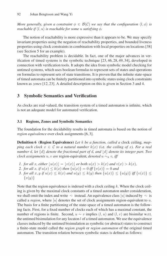
Timed Automata: Semantics, Algorithms and Tools 93
y
x
Fig. 2. Regions for a System with Two Clocks.
– 〈l, [u]〉 ⇒ 〈l, [v]〉 if 〈l, u〉 d−→ 〈l, v〉 for a positive real number d and– 〈l, [u]〉 ⇒ 〈l′, [v]〉 if 〈l, u〉 a−→ 〈l′, v〉 for an action a.
Note that the transition relation ⇒ is finite. Thus the region graph for a timed au-tomaton is finite. Several verification problems such as reachability analysis, untimedlanguage inclusion, language emptiness [6] as well as timed bisimulation [19] can besolved by techniques based on the region construction.
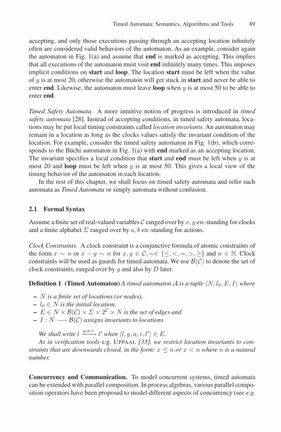
However, the problem with region graphs is the potential explosion in the numberof regions. In fact, it is exponential in the number of clocks as well as the maximalconstants appearing in the guards of an automaton. As an example, consider Fig. 2. Thefigure shows the possible regions in each location of an automaton with two clocks xand y. The largest number compared to x is 3, and the largest number compared to yis 2. In the figure, all corner points (intersections), line segments, and open areas areregions. Thus, the number of possible regions in each location of this example is 60.
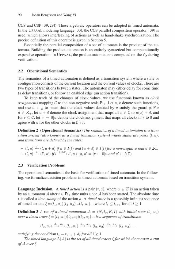
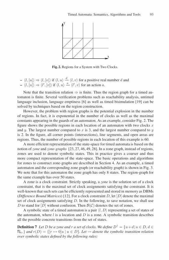
A more efficient representation of the state-space for timed automata is based on thenotion of zone and zone-graphs [23, 27, 46, 49, 28]. In a zone graph, instead of regions,zones are used to denote symbolic states. This in practice gives a coarser and thusmore compact representation of the state-space. The basic operations and algorithmsfor zones to construct zone-graphs are described in Section 4. As an example, a timedautomaton and the corresponding zone graph (or reachability graph) is shown in Fig. 3.We note that for this automaton the zone graph has only 8 states. The region-graph forthe same example has over 50 states.
A zone is a clock constraint. Strictly speaking, a zone is the solution set of a clockconstraint, that is the maximal set of clock assignments satisfying the constraint. It iswell-known that such sets can be efficiently represented and stored in memory as DBMs(Difference Bound Matrices) [12]. For a clock constraintD, let [D] denote the maximalset of clock assignments satisfying D. In the following, to save notation, we shall useD to stand for [D] without confusion. Then B(C) denotes the set of zones.
A symbolic state of a timed automaton is a pair 〈l, D〉 representing a set of states ofthe automaton, where l is a location and D is a zone. A symbolic transition describesall the possible concrete transitions from the set of states.
Definition 7 LetD be a zone and r a set of clocks. We defineD↑ = {u+d |u ∈ D, d ∈�+} and r(D) = {[r → 0]u | u ∈ D}. Let� denote the symbolic transition relationover symbolic states defined by the following rules:
94 Johan Bengtsson and Wang Yi
off
dim
bright
press?x:=0
x<=10press?
x>10press?
press?
� off, x = 0 �
〈off, x ≥ 0〉
〈off, x > 10〉
〈dim, x = 0〉
〈dim, x ≥ 0〉〈bright, x = 0〉
〈bright, x ≤ 10〉
〈bright, x ≥ 0〉
Fig. 3. A Timed Automaton and its Zone Graph.
– 〈l, D〉� ⟨l, D↑ ∧ I(l)⟩
– 〈l, D〉� 〈l′, r(D ∧ g) ∧ I(l′)〉 if lg,a,r−−−→ l′
We shall study these operations in details in Section 4 whereD↑ is written as up(D)and r(D) as reset(D, r := 0). It will be shown that the set of zones B(C) is closed un-der these operations, in the sense that the result of the operations is also a zone. Anotherimportant property of zones is that a zone has a canonical form. A zoneD is closed un-der entailment or just closed for short, if no constraint inD can be strengthened withoutreducing the solution set. The canonicity of zones means that for each zone D ∈ B(C),there is a unique zoneD′ ∈ B(C) such thatD andD′ have exactly the same solution setand D′ is closed under entailment. Section 4 describes how to compute and representthe canonical form of a zone. It is the key structure for the efficient implementation ofstate-space exploration using the symbolic semantics.
The symbolic semantics corresponds closely to the operational semantics in thesense that 〈l, D〉 � 〈l′, D′〉 implies for all u′ ∈ D′, 〈l, u〉 → 〈l′, u′〉 for some u ∈ D.More generally, the symbolic semantics is a correct and full characterization of theoperational semantics given in Definition 2.
Theorem 1 Assume a timed automaton with initial state 〈l0, u0〉.1. (soundness) 〈l0, {u0}〉�∗ 〈lf , Df 〉 implies 〈l0, u0〉 →∗ 〈lf , uf 〉 for all uf ∈ Df .2. (Completeness) 〈l0, u0〉 →∗ 〈lf , uf 〉 implies 〈l0, {u0}〉 �∗ 〈lf , Df〉 for some Df
such that uf ∈ Df
The soundness means that if the initial symbolic state 〈l0, {u0}〉 may lead to a set offinal states 〈lf , Df〉 according to�, all the final states should be reachable according tothe concrete operational semantics. The completeness means that if a state is reachableaccording to the concrete operational semantics, it should be possible to conclude thisusing the symbolic transition relation.
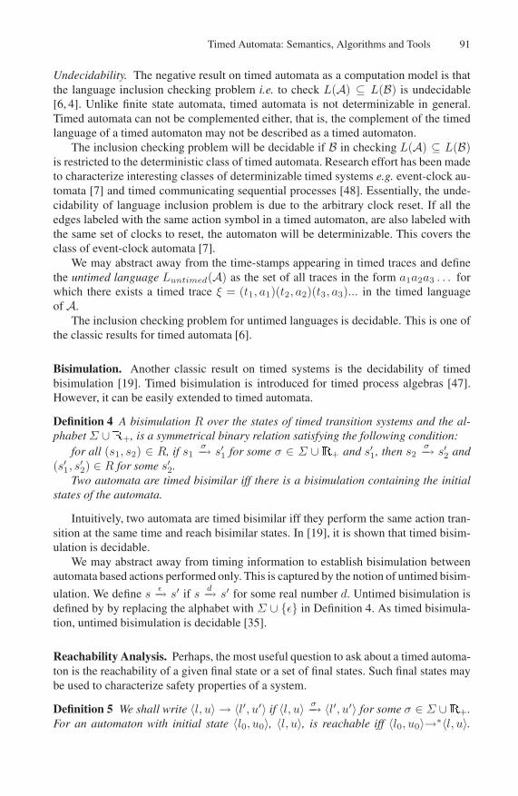
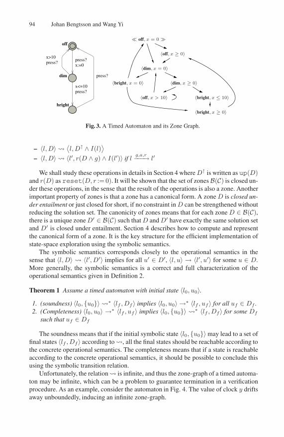
Unfortunately, the relation� is infinite, and thus the zone-graph of a timed automa-ton may be infinite, which can be a problem to guarantee termination in a verificationprocedure. As an example, consider the automaton in Fig. 4. The value of clock y driftsaway unboundedly, inducing an infinite zone-graph.
Timed Automata: Semantics, Algorithms and Tools 95
start
loopx<=10
end
x:=0,y:=0
y>=20x:=0,y:=0
x==10x:=0
� start, x = y �
〈loop, x ≤ 10 ∧ x = y〉
〈loop, x ≤ 10 ∧ y ≤ 20 ∧ y − x = 10〉
〈loop, x ≤ 10 ∧ y ≤ 30 ∧ y − x = 20〉
〈loop, x ≤ 10 ∧ y ≤ 40 ∧ y − x = 30〉
〈end, x = y〉...
Fig. 4. A Timed Automaton with an Infinite Zone-Graph.
The solution is to transform (i.e. normalize) zones that may contain arbitrarily largeconstants to their representatives in a class of zones whose constants are bounded byfixed constants e.g. the maximal clock constants appearing in the automaton, using anabstraction technique similar to the widening operation [26]. The intuition is that oncethe value of a clock is larger than the maximal constant in the automaton, it is no longerimportant to know the precise value of the clock, but only the fact that it is above theconstant.
3.2 Zone-Normalization for Automata without Difference Constraints
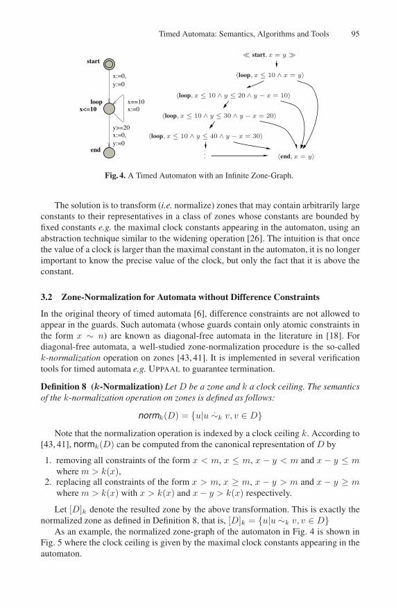
In the original theory of timed automata [6], difference constraints are not allowed toappear in the guards. Such automata (whose guards contain only atomic constraints inthe form x ∼ n) are known as diagonal-free automata in the literature in [18]. Fordiagonal-free automata, a well-studied zone-normalization procedure is the so-calledk-normalization operation on zones [43, 41]. It is implemented in several verificationtools for timed automata e.g. UPPAAL to guarantee termination.
Definition 8 (k-Normalization) Let D be a zone and k a clock ceiling. The semanticsof the k-normalization operation on zones is defined as follows:
normk(D) = {u|u .∼k v, v ∈ D}Note that the normalization operation is indexed by a clock ceiling k. According to
[43, 41], normk(D) can be computed from the canonical representation of D by
1. removing all constraints of the form x < m, x ≤ m, x − y < m and x − y ≤ mwhere m > k(x),
2. replacing all constraints of the form x > m, x ≥ m, x − y > m and x − y ≥ mwhere m > k(x) with x > k(x) and x− y > k(x) respectively.
Let [D]k denote the resulted zone by the above transformation. This is exactly thenormalized zone as defined in Definition 8, that is, [D]k = {u|u .∼k v, v ∈ D}
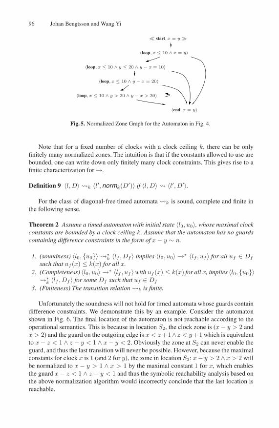
As an example, the normalized zone-graph of the automaton in Fig. 4 is shown inFig. 5 where the clock ceiling is given by the maximal clock constants appearing in theautomaton.
96 Johan Bengtsson and Wang Yi
� start, x = y �
〈loop, x ≤ 10 ∧ x = y〉
〈loop, x ≤ 10 ∧ y ≤ 20 ∧ y − x = 10〉
〈loop, x ≤ 10 ∧ y − x = 20〉
〈loop, x ≤ 10 ∧ y > 20 ∧ y − x > 20〉
〈end, x = y〉
Fig. 5. Normalized Zone Graph for the Automaton in Fig. 4.
Note that for a fixed number of clocks with a clock ceiling k, there can be onlyfinitely many normalized zones. The intuition is that if the constants allowed to use arebounded, one can write down only finitely many clock constraints. This gives rise to afinite characterization for →.
Definition 9 〈l, D〉�k 〈l′, normk(D′)〉 if 〈l, D〉� 〈l′, D′〉.
For the class of diagonal-free timed automata�k is sound, complete and finite inthe following sense.
Theorem 2 Assume a timed automaton with initial state 〈l0, u0〉, whose maximal clockconstants are bounded by a clock ceiling k. Assume that the automaton has no guardscontaining difference constraints in the form of x− y ∼ n.
1. (soundness) 〈l0, {u0}〉 �∗k 〈lf , Df 〉 implies 〈l0, u0〉 →∗ 〈lf , uf 〉 for all uf ∈ Df
such that uf(x) ≤ k(x) for all x.2. (Completeness) 〈l0, u0〉 →∗ 〈lf , uf 〉 with uf(x) ≤ k(x) for all x, implies 〈l0, {u0}〉�∗
k 〈lf , Df 〉 for some Df such that uf ∈ Df
3. (Finiteness) The transition relation�k is finite.
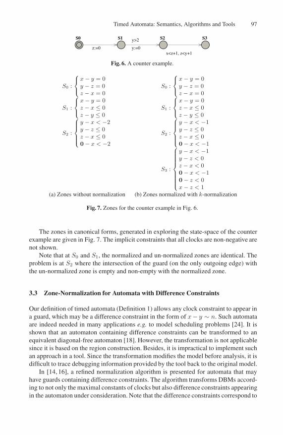
Unfortunately the soundness will not hold for timed automata whose guards containdifference constraints. We demonstrate this by an example. Consider the automatonshown in Fig. 6. The final location of the automaton is not reachable according to theoperational semantics. This is because in location S2, the clock zone is (x− y > 2 andx > 2) and the guard on the outgoing edge is x < z+1∧z < y+1 which is equivalentto x− z < 1 ∧ z − y < 1 ∧ x− y < 2. Obviously the zone at S2 can never enable theguard, and thus the last transition will never be possible. However, because the maximalconstants for clock x is 1 (and 2 for y), the zone in location S2: x− y > 2∧ x > 2 willbe normalized to x − y > 1 ∧ x > 1 by the maximal constant 1 for x, which enablesthe guard x − z < 1 ∧ z − y < 1 and thus the symbolic reachability analysis based onthe above normalization algorithm would incorrectly conclude that the last location isreachable.
Timed Automata: Semantics, Algorithms and Tools 97
S0 S1 S2 S3
z:=0
y>2
y:=0x<z+1, z<y+1
Fig. 6. A counter example.
S0 :
x − y = 0y − z = 0z − x = 0
S1 :
x − y = 0z − x ≤ 0z − y ≤ 0
S2 :
y − x < −2y − z ≤ 0z − x ≤ 00 − x < −2
S0 :
x − y = 0y − z = 0z − x = 0
S1 :
x − y = 0z − x ≤ 0z − y ≤ 0
S2 :
y − x < −1y − z ≤ 0z − x ≤ 00 − x < −1
S3 :
y − x < −1y − z < 0z − x < 00 − x < −10 − z < 0x − z < 1
(a) Zones without normalization (b) Zones normalized with k-normalization
Fig. 7. Zones for the counter example in Fig. 6.
The zones in canonical forms, generated in exploring the state-space of the counterexample are given in Fig. 7. The implicit constraints that all clocks are non-negative arenot shown.
Note that at S0 and S1, the normalized and un-normalized zones are identical. Theproblem is at S2 where the intersection of the guard (on the only outgoing edge) withthe un-normalized zone is empty and non-empty with the normalized zone.
3.3 Zone-Normalization for Automata with Difference Constraints
Our definition of timed automata (Definition 1) allows any clock constraint to appear ina guard, which may be a difference constraint in the form of x− y ∼ n. Such automataare indeed needed in many applications e.g. to model scheduling problems [24]. It isshown that an automaton containing difference constraints can be transformed to anequivalent diagonal-free automaton [18]. However, the transformation is not applicablesince it is based on the region construction. Besides, it is impractical to implement suchan approach in a tool. Since the transformation modifies the model before analysis, it isdifficult to trace debugging information provided by the tool back to the original model.
In [14, 16], a refined normalization algorithm is presented for automata that mayhave guards containing difference constraints. The algorithm transforms DBMs accord-ing to not only the maximal constants of clocks but also difference constraints appearingin the automaton under consideration. Note that the difference constraints correspond to
98 Johan Bengtsson and Wang Yi
the diagonal lines which split the entire space of clock assignments. A finer partitioningis needed.
We present the semantical characterization for the refined normalization operationbased on a refined version of the region equivalence from Definition 6.
Definition 10 (Normalization Using Difference Constraints) Let G stand for a finiteset of difference constraints of the form x−y ∼ n for x, y ∈ C,∼∈ {≤, <,=, >,≥} andn ∈ N, and k for a clock ceiling. Two clock assignments u, v are equivalent, denotedu
.∼k,G v if the following holds:
– u.∼k v and
– for all g ∈ G, u ∈ g iff v ∈ g.
The semantics of the refined k-normalization operation on zones is defined as follows:
normk,G(D) = {u|u .∼k,G v, v ∈ D}
Note that the refined region equivalence is indexed by both a clock ceiling k and a finiteset of difference constraints G, and so is the normalization operation.
Since the number of regions induced by.∼k is finite and there are only finitely
many constraints in G,.∼k,G induces finitely many equivalence classes. Thus for any
given zone D, normk,G(D) is well-defined in the sense that it contains only a finite setof equivalence classes though the set may not be a convex zone, and it can be computedeffectively according to the refined regions. In general, normk,G(D) is a non-convexzone, which can be implemented as the union of a finite list of convex zones. The nextsection will show how to compute this efficiently.
The refined zone-normalization gives rise to a finite characterization for →.
Definition 11 〈l, D〉�k,G 〈l′, normk,G(D′)〉 if 〈l, D〉� 〈l′, D′〉.
The following states the correctness and finiteness of�k,G .
Theorem 3 Assume a timed automaton with initial state 〈l0, u0〉, whose maximal clockconstants are bounded by a clock ceiling k, and whose guards contain only a finite setof difference constraints denoted G.
1. (soundness) 〈l0, {u0}〉 (�k,G)∗ 〈lf , Df 〉 implies 〈l0, u0〉 →∗ 〈lf , uf〉 for all uf ∈Df such that uf (x) ≤ k(x) for all x.
2. (Completeness) 〈l0, u0〉 →∗ 〈lf , uf〉 with uf(x) ≤ k(x) for all x implies 〈l0, {u0}〉(�k,G)∗ 〈lf , Df〉 for some Df such that uf ∈ Df
3. (Finiteness) The transition relation�k,G is finite.
3.4 Symbolic Reachability Analysis
Model-checking concerns two types of properties liveness and safety. The essentialalgorithm of checking liveness properties is loop detection, which is computationallyexpensive. The main effort on verification of timed systems has been put on safety
Timed Automata: Semantics, Algorithms and Tools 99
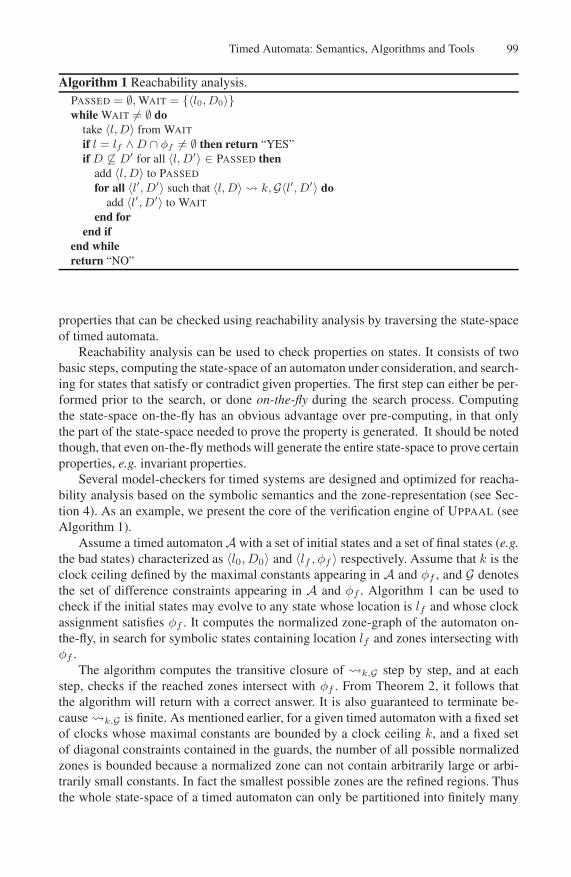
Algorithm 1 Reachability analysis.PASSED = ∅, WAIT = {〈l0, D0〉}while WAIT �= ∅ do
take 〈l, D〉 from WAIT
if l = lf ∧ D ∩ φf �= ∅ then return “YES”if D �⊆ D′ for all 〈l, D′〉 ∈ PASSED then
add 〈l, D〉 to PASSED
for all 〈l′, D′〉 such that 〈l, D〉� k, G〈l′, D′〉 doadd 〈l′, D′〉 to WAIT
end forend if
end whilereturn “NO”
properties that can be checked using reachability analysis by traversing the state-spaceof timed automata.
Reachability analysis can be used to check properties on states. It consists of twobasic steps, computing the state-space of an automaton under consideration, and search-ing for states that satisfy or contradict given properties. The first step can either be per-formed prior to the search, or done on-the-fly during the search process. Computingthe state-space on-the-fly has an obvious advantage over pre-computing, in that onlythe part of the state-space needed to prove the property is generated. It should be notedthough, that even on-the-fly methods will generate the entire state-space to prove certainproperties, e.g. invariant properties.
Several model-checkers for timed systems are designed and optimized for reacha-bility analysis based on the symbolic semantics and the zone-representation (see Sec-tion 4). As an example, we present the core of the verification engine of UPPAAL (seeAlgorithm 1).
Assume a timed automaton A with a set of initial states and a set of final states (e.g.the bad states) characterized as 〈l0, D0〉 and 〈lf , φf 〉 respectively. Assume that k is theclock ceiling defined by the maximal constants appearing in A and φf , and G denotesthe set of difference constraints appearing in A and φf . Algorithm 1 can be used tocheck if the initial states may evolve to any state whose location is lf and whose clockassignment satisfies φf . It computes the normalized zone-graph of the automaton on-the-fly, in search for symbolic states containing location lf and zones intersecting withφf .
The algorithm computes the transitive closure of �k,G step by step, and at eachstep, checks if the reached zones intersect with φf . From Theorem 2, it follows thatthe algorithm will return with a correct answer. It is also guaranteed to terminate be-cause�k,G is finite. As mentioned earlier, for a given timed automaton with a fixed setof clocks whose maximal constants are bounded by a clock ceiling k, and a fixed setof diagonal constraints contained in the guards, the number of all possible normalizedzones is bounded because a normalized zone can not contain arbitrarily large or arbi-trarily small constants. In fact the smallest possible zones are the refined regions. Thusthe whole state-space of a timed automaton can only be partitioned into finitely many
100 Johan Bengtsson and Wang Yi
symbolic states and the worst case is the size of the region graph of the automaton, in-duced by the refined region equivalence. Therefore, the algorithm is working on a finitestructure and it will terminate.
Algorithm 1 also highlights some of the issues in developing a model-checker fortimed automata. Firstly, the representation and manipulation of states, primarily zones,is crucial to the performance of a model-checker. Note that in addition to the opera-tions to compute the successors of a zone according to �k,G , the algorithm uses twomore operations to check the emptiness of a zone as well as the inclusion betweentwo zones. Thus, designing efficient algorithms and data-structures for zones is a majorissue in developing a verification tool for timed automata, which is addressed in Sec-tion 4. Secondly, PASSED holds all encountered states and its size puts a limit on thesize of systems we can verify. This raises the research challenges e.g. state compression[14], state-space reduction [15] and approximate techniques [9].
4 DBM: Algorithms and Data Structures
The preceding section presents the key elements needed in symbolic reachability anal-ysis. Recall that the operations on zones are all defined in terms of sets of clock assign-ments. It is not clear how to compute the result of such an operation. In this section, wedescribe how to represent zones, compute the operations and check properties on zones.Pseudo code for the operations is given in the appendix.
4.1 DBM Basics
Recall that a clock constraint over C is a conjunction of atomic constraints of the formx ∼ m and x − y ∼ n where x, y ∈ C, ∼∈ {≤, <,=, >,≥} and m,n ∈ N. A zonedenoted by a clock constraint D is the maximal set of clock assignments satisfying D.The most important property of zones is that they can can be represented as matrices i.e.DBMs (Difference Bound Matrices) [12, 23], which have a canonical representation.In the following, we describe the basic structure and properties of DBMs.
To have a unified form for clock constraints we introduce a reference clock 0 withthe constant value 0. Let C0 = C ∪ {0}. Then any zone D ∈ B(C) can be rewritten as aconjunction of constraints of the form x− y � n for x, y ∈ C0, �∈ {<,≤} and n ∈ �.
Naturally, if the rewritten zone has two constraints on the same pair of variablesonly the intersection of the two is significant. Thus, a zone can be represented usingat most |C0|2 atomic constraints of the form x − y � n such that each pair of clocksx− y is mentioned only once. We can then store zones using |C0|× |C0| matrices whereeach element in the matrix corresponds to an atomic constraint. Since each elementin such a matrix represents a bound on the difference between two clocks, they arenamed Difference Bound Matrices (DBMs). In the following presentation, we use Dij
to denote element (i, j) in the DBM representing the zone D.To construct the DBM representation for a zoneD, we start by numbering all clocks
in C0 as 0, . . . , n and the index for 0 is 0. Let each clock be denoted by one row in thematrix. The row is used for storing lower bounds on the difference between the clockand all other clocks, and thus the corresponding column is used for upper bounds. Theelements in the matrix are then computed in three steps.
Timed Automata: Semantics, Algorithms and Tools 101
– For each constraint xi − xj � n of D, let Dij = (n,�).– For each clock difference xi − xj that is unbounded in D, let Dij = ∞. Where ∞
is a special value denoting that no bound is present.– Finally add the implicit constraints that all clocks are positive, i.e. 0− xi ≤ 0, and
that the difference between a clock and itself is always 0, i.e. xi − xi ≤ 0.
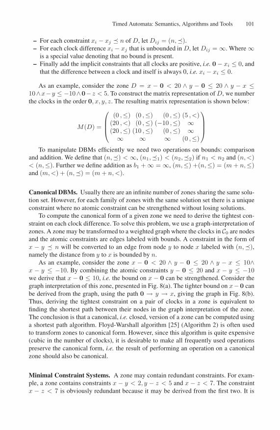
As an example, consider the zone D = x − 0 < 20 ∧ y − 0 ≤ 20 ∧ y − x ≤10∧x−y ≤ −10∧0−z < 5. To construct the matrix representation ofD, we numberthe clocks in the order 0, x, y, z. The resulting matrix representation is shown below:
M(D) =
(0 ,≤) (0 ,≤) (0 ,≤) (5 ,<)(20 ,<) (0 ,≤) (−10 ,≤) ∞(20 ,≤) (10 ,≤) (0 ,≤) ∞
∞ ∞ ∞ (0 ,≤)
To manipulate DBMs efficiently we need two operations on bounds: comparisonand addition. We define that (n,�) < ∞, (n1,�1) < (n2,�2) if n1 < n2 and (n,<)< (n,≤). Further we define addition as b1 + ∞ = ∞, (m,≤) +(n,≤) = (m+ n,≤)and (m,<) + (n,�) = (m+ n,<).
Canonical DBMs. Usually there are an infinite number of zones sharing the same solu-tion set. However, for each family of zones with the same solution set there is a uniqueconstraint where no atomic constraint can be strengthened without losing solutions.
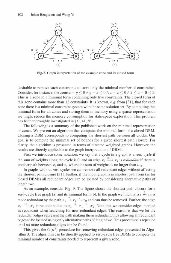
To compute the canonical form of a given zone we need to derive the tightest con-straint on each clock difference. To solve this problem, we use a graph-interpretation ofzones. A zone may be transformed to a weighted graph where the clocks in C0 are nodesand the atomic constraints are edges labeled with bounds. A constraint in the form ofx − y � n will be converted to an edge from node y to node x labeled with (n,�),namely the distance from y to x is bounded by n.
As an example, consider the zone x − 0 < 20 ∧ y − 0 ≤ 20 ∧ y − x ≤ 10∧x − y ≤ −10. By combining the atomic constraints y − 0 ≤ 20 and x − y ≤ −10we derive that x − 0 ≤ 10, i.e. the bound on x − 0 can be strengthened. Consider thegraph interpretation of this zone, presented in Fig. 8(a). The tighter bound on x−0 canbe derived from the graph, using the path 0 → y → x, giving the graph in Fig. 8(b).Thus, deriving the tightest constraint on a pair of clocks in a zone is equivalent tofinding the shortest path between their nodes in the graph interpretation of the zone.The conclusion is that a canonical, i.e. closed, version of a zone can be computed usinga shortest path algorithm. Floyd-Warshall algorithm [25] (Algorithm 2) is often usedto transform zones to canonical form. However, since this algorithm is quite expensive(cubic in the number of clocks), it is desirable to make all frequently used operationspreserve the canonical form, i.e. the result of performing an operation on a canonicalzone should also be canonical.
Minimal Constraint Systems. A zone may contain redundant constraints. For exam-ple, a zone contains constraints x − y < 2, y − z < 5 and x − z < 7. The constraintx − z < 7 is obviously redundant because it may be derived from the first two. It is
102 Johan Bengtsson and Wang Yi
�
� �
�����
������
��������
���
�����������
�����
�������
�����
�
� �
�����
������
��������
���
�����������
�����
�������
�����
(a) (b)
Fig. 8. Graph interpretation of the example zone and its closed form.
desirable to remove such constraints to store only the minimal number of constraints.Consider, for instance, the zone x− y ≤ 0 ∧ y − z ≤ 0 ∧ z − x ≤ 0 ∧ 2 ≤ x− 0 ≤ 3.This is a zone in a minimal form containing only five constraints. The closed form ofthis zone contains more than 12 constraints. It is known, e.g. from [31], that for eachzone there is a minimal constraint system with the same solution set. By computing thisminimal form for all zones and storing them in memory using a sparse representationwe might reduce the memory consumption for state-space exploration. This problemhas been thoroughly investigated in [31, 41, 36].
The following is a summary of the published work on the minimal representationof zones. We present an algorithm that computes the minimal form of a closed DBM.Closing a DBM corresponds to computing the shortest path between all clocks. Ourgoal is to compute the minimal set of bounds for a given shortest path closure. Forclarity, the algorithm is presented in terms of directed weighted graphs. However, theresults are directly applicable to the graph interpretation of DBMs.
First we introduce some notation: we say that a cycle in a graph is a zero cycle ifthe sum of weights along the cycle is 0, and an edge xi
nij−−→ xj is redundant if there isanother path between xi and xj where the sum of weights is no larger than nij .
In graphs without zero cycles we can remove all redundant edges without affectingthe shortest path closure [31]. Further, if the input graph is in shortest path form (as forclosed DBMs) all redundant edges can be located by considering alternative paths oflength two.
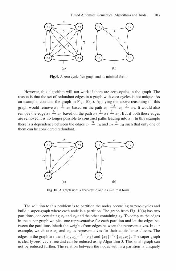
As an example, consider Fig. 9. The figure shows the shortest path closure for a
zero-cycle free graph (a) and its minimal form (b). In the graph we find that x19−→ x2 is
made redundant by the path x17−→ x4
2−→ x2 and can thus be removed. Further, the edge
x315−→ x2 is redundant due to x3
5−→ x19−→ x2. Note that we consider edges marked
as redundant when searching for new redundant edges. The reason is that we let theredundant edges represent the path making them redundant, thus allowing all redundantedges to be located using only alternative paths of length two. This procedure is repeateduntil no more redundant edges can be found.
This gives the O(n3) procedure for removing redundant edges presented in Algo-rithm 3. The algorithm can be directly applied to zero-cycle free DBMs to compute theminimal number of constraints needed to represent a given zone.
Timed Automata: Semantics, Algorithms and Tools 103
x1 x2
x3 x4
9
8
7
5
13
126
15
13
7
2
1
x1 x2
x3 x4
7
5
6 2
1
(a) (b)
Fig. 9. A zero cycle free graph and its minimal form.
However, this algorithm will not work if there are zero-cycles in the graph. Thereason is that the set of redundant edges in a graph with zero-cycles is not unique. Asan example, consider the graph in Fig. 10(a). Applying the above reasoning on this
graph would remove x13−→ x3 based on the path x1
−2−−→ x25−→ x3. It would also
remove the edge x25−→ x3 based on the path x2
2−→ x13−→ x3. But if both these edges
are removed it is no longer possible to construct paths leading into x3. In this example
there is a dependence between the edges x13−→ x3 and x2
5−→ x3 such that only one ofthem can be considered redundant.
x1 x2
x3
-2
3
2
5
3
1
x1 x2
x3
-2
3
2
3
(a) (b)
Fig. 10. A graph with a zero-cycle and its minimal form.
The solution to this problem is to partition the nodes according to zero-cycles andbuild a super-graph where each node is a partition. The graph from Fig. 10(a) has twopartitions, one containing x1 and x2 and the other containing x3. To compute the edgesin the super-graph we pick one representative for each partition and let the edges be-tween the partitions inherit the weights from edges between the representatives. In ourexample, we choose x1 and x3 as representatives for their equivalence classes. The
edges in the graph are then {x1, x2} 3−→ {x3} and {x3} 3−→ {x1, x2}. The super-graphis clearly zero-cycle free and can be reduced using Algorithm 3. This small graph cannot be reduced further. The relation between the nodes within a partition is uniquely
104 Johan Bengtsson and Wang Yi
defined by the zero-cycle and all other edges may be removed. In our example all edgeswithin each equivalence class are part of the zero-cycle and thus none of them canbe removed. Finally the reduced super-graph is connected to the reduced partitions. Inour example we end up with the graph in Fig. 10(b). Pseudo-code for the reduction-procedure is shown in Algorithm 4.
Now we have an algorithm for computing the minimal number of edges to repre-sent a given shortest path closure that can be used to compute the minimal number ofconstraints needed to represent a given zone.
4.2 Basic Operations on DBMs
This subsection presents all the basic operations on DBMs except the ones for zone-normalization, needed in symbolic state space exploration of timed automata, both forforwards and backwards analysis. The two operations for zone-normalization are pre-sented in the next subsection.
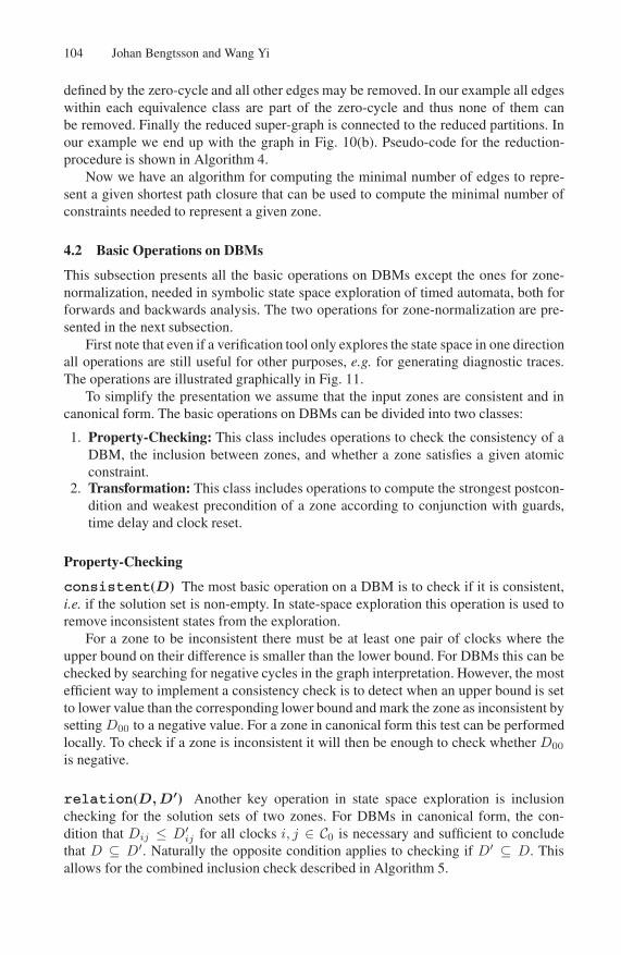
First note that even if a verification tool only explores the state space in one directionall operations are still useful for other purposes, e.g. for generating diagnostic traces.The operations are illustrated graphically in Fig. 11.
To simplify the presentation we assume that the input zones are consistent and incanonical form. The basic operations on DBMs can be divided into two classes:
1. Property-Checking: This class includes operations to check the consistency of aDBM, the inclusion between zones, and whether a zone satisfies a given atomicconstraint.
2. Transformation: This class includes operations to compute the strongest postcon-dition and weakest precondition of a zone according to conjunction with guards,time delay and clock reset.
Property-Checking
consistent(D) The most basic operation on a DBM is to check if it is consistent,i.e. if the solution set is non-empty. In state-space exploration this operation is used toremove inconsistent states from the exploration.
For a zone to be inconsistent there must be at least one pair of clocks where theupper bound on their difference is smaller than the lower bound. For DBMs this can bechecked by searching for negative cycles in the graph interpretation. However, the mostefficient way to implement a consistency check is to detect when an upper bound is setto lower value than the corresponding lower bound and mark the zone as inconsistent bysetting D00 to a negative value. For a zone in canonical form this test can be performedlocally. To check if a zone is inconsistent it will then be enough to check whether D00
is negative.
relation(D,D′) Another key operation in state space exploration is inclusionchecking for the solution sets of two zones. For DBMs in canonical form, the con-dition that Dij ≤ D′
ij for all clocks i, j ∈ C0 is necessary and sufficient to concludethat D ⊆ D′. Naturally the opposite condition applies to checking if D′ ⊆ D. Thisallows for the combined inclusion check described in Algorithm 5.
Timed Automata: Semantics, Algorithms and Tools 105
y
x
y
x
y
x
y
x
y
x
y
xD
y
xreset(D,x := 2)
y
x
y
x
up(D) down(D)
and(D,x ≤ 2) normk(D) shift(D, y := y + 1)
free(D, y) copy(D,x := y)
Fig. 11. DBM operations applied to the same zone where for normk(D), k is defined by k(x) =2 and k(y) = 1.
satisfied(D,xi −xj � m) Sometimes it is desirable to non-destructively checkif a zone satisfies a constraint, i.e. to check if the zone D ∧ xi − xj � m is consistentwithout altering D. From the definition of the consistent-operation we know thata zone is consistent if it has no negative cycles. Thus, checking if D ∧ xi − xj � mis non-empty can be done by checking if adding the guard to the zone would introducea negative cycle. For a DBM on canonical form this test can be performed locally bychecking if (m,�) +Dji is negative.
Transformations
up(D) The up operation computes the strongest postcondition of a zone with respectto delay, i.e. up(D) contains the clock assignments that can be reached from D bydelay. Formally, this operation is defined as up(D) = {u+ d | u ∈ D, d ∈ �+}.
Algorithmically, up is computed by removing the upper bounds on all individualclocks (In a DBM all elements Di0 are set to ∞). This is the same as saying that any
106 Johan Bengtsson and Wang Yi
clock assignment in a given zone may delay an arbitrary amount of time. The propertythat all clocks proceed at the same speed is ensured by the fact that constraints on thedifferences between clocks are not altered by the operation.
This operation preserves the canonical form, i.e. applying up to a canonical DBMwill result in a new canonical DBM. The up operation is also presented in Algorithm 6.
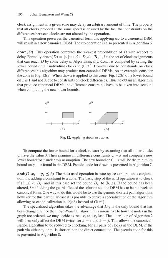
down(D) This operation computes the weakest precondition of D with respect todelay. Formally down(D) = {u |u+d ∈ D, d ∈ �+}, i.e. the set of clock assignmentsthat can reach D by some delay d. Algorithmically, down is computed by setting thelower bound on all individual clocks to (0,≤). However due to constraints on clockdifferences this algorithm may produce non-canonical DBMs. As an example, considerthe zone in Fig. 12(a). When down is applied to this zone (Fig. 12(b)), the lower boundon x is 1 and not 0, due to constraints on clock differences. Thus, to obtain an algorithmthat produce canonical DBMs the difference constraints have to be taken into accountwhen computing the new lower bounds.
y y
(a) (b)
x x
Fig. 12. Applying down to a zone.
To compute the lower bound for a clock x, start by assuming that all other clocksyi have the value 0. Then examine all difference constraints yi − x and compute a newlower bound for x under this assumption. The new bound on 0−x will be the minimumbound on yi−x found in the DBM. Pseudo-code for down is presented in Algorithm 7.
and(D, xi − yj � b) The most used operation in state-space exploration is conjunc-tion, i.e. adding a constraint to a zone. The basic step of the and operation is to checkif (b,�) < Dij and in this case set the bound Dij to (b,�). If the bound has beenaltered, i.e. if adding the guard affected the solution set, the DBM has to be put back oncanonical form. One way to do this would be to use the generic shortest path algorithm,however for this particular case it is possible to derive a specialization of the algorithmallowing re-canonicalization in O(n2) instead of O(n3).
The specialized algorithm takes the advantage that Dij is the only bound that hasbeen changed. Since the Floyd-Warshall algorithm is insensitive to how the nodes in thegraph are ordered, we may decide to treat xi and xj last. The outer loop of Algorithm 2will then only affect the DBM twice, for k = i and k = j. This allows the canonical-isation algorithm to be reduced to checking, for all pairs of clocks in the DBM, if thepath via either xi or xj is shorter than the direct connection. The pseudo code for thisis presented in Algorithm 8.
Timed Automata: Semantics, Algorithms and Tools 107
free(D, x) The free operation removes all constraints on a given clock, i.e. theclock may take any positive value. Formally this is expressed as free(D,x) = {u[x =d] | u ∈ D, d ∈ �+}. In state-space exploration this operation is used in combinationwith conjunction, to implement reset operations on clocks. It can be used in both for-wards and backwards exploration, but since forwards exploration allows other moreefficient implementations of reset, free is only used when exploring the state-spacebackwards.
A simple algorithm for this operation is to remove all bounds on x in the DBMand set D0x = (0,≤). However, the result may not be on canonical form. To obtainan algorithm preserving the canonical form, we change how new difference constraintsregarding x are derived. We note that the constraint 0 − x ≤ 0 can be combined withconstraints of the form y − 0 � m to compute new bounds for y − x. For instance,if y − 0 ≤ 5 we can derive that y − x ≤ 5. To obtain a DBM on canonical form wederive bounds for Dyx based on Dy0 instead of setting Dyx = ∞.In Algorithm 9 thisis presented as pseudo code.
reset(D, x := m) In forwards exploration this operation is used to set clocks tospecific values, i.e. reset(D,x :=m) = {u[x = m] | u ∈ D}. Without the require-ment that output should be on canonical form, reset can be implemented by settingDx0 = (m,≤), D0x = (−m,≤) and remove all other bounds on x. However, if weinstead of removing the difference constraints compute new values using constraints onthe other clocks, like in the implementation of free, we obtain an implementation thatpreserve the canonical form. Such an implementation is presented in Algorithm 10.
copy(D, x := y) This is another operation used in forwards state-space exploration.It copies the value of one clock to another. Formally, we define copy(D,x := y) as{u[x = u(y)] | u ∈ D}. As reset, copy can be implemented by assigning Dxy =(0,≤), Dyx = (0,≤), removing all other bounds on x and re-canonicalize the zone.However, a more efficient implementation is obtained by assigning Dxy = (0,≤),Dyx = (0,≤) and then copy the rest of the bounds on x from y. For pseudo code, seeAlgorithm 11.
shift(D, x := x + m) The last reset operation is shifting a clock, i.e. adding orsubtracting a clock with an integer value, i.e. shift(D,x :=x+m) = {u[x = u(x)+m] | u ∈ D}. The definition gives a hint on how to implement the operation. We canview the shift operation as a substitution of x−m for x in the zone. With this reasoningm is added to the upper and lower bounds of x. However, since lower bounds on xare represented by constraints on y − x, m is subtracted from all those bounds. Thisoperation is presented in pseudo-code in Algorithm 12.
4.3 Zone-Normalization
The operations for zone-normalization are to transform zones which may contain arbi-trarily large constants to zones containing only bounded constants in order to obtain afinite zone-graph.
108 Johan Bengtsson and Wang Yi
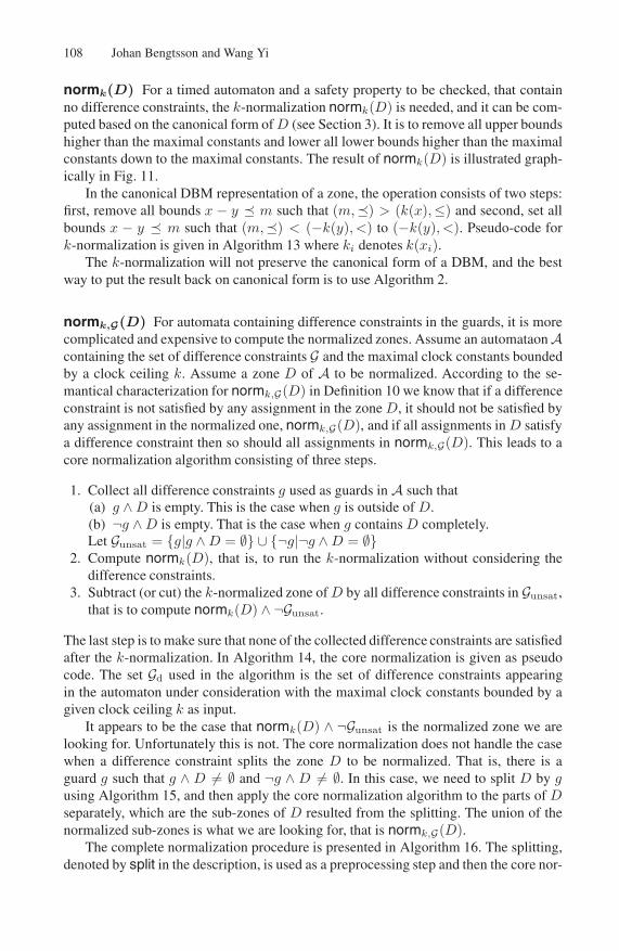
normk(D) For a timed automaton and a safety property to be checked, that containno difference constraints, the k-normalization normk(D) is needed, and it can be com-puted based on the canonical form ofD (see Section 3). It is to remove all upper boundshigher than the maximal constants and lower all lower bounds higher than the maximalconstants down to the maximal constants. The result of normk(D) is illustrated graph-ically in Fig. 11.
In the canonical DBM representation of a zone, the operation consists of two steps:first, remove all bounds x − y � m such that (m,�) > (k(x),≤) and second, set allbounds x − y � m such that (m,�) < (−k(y), <) to (−k(y), <). Pseudo-code fork-normalization is given in Algorithm 13 where ki denotes k(xi).
The k-normalization will not preserve the canonical form of a DBM, and the bestway to put the result back on canonical form is to use Algorithm 2.
normk,G(D) For automata containing difference constraints in the guards, it is morecomplicated and expensive to compute the normalized zones. Assume an automataonAcontaining the set of difference constraints G and the maximal clock constants boundedby a clock ceiling k. Assume a zone D of A to be normalized. According to the se-mantical characterization for normk,G(D) in Definition 10 we know that if a differenceconstraint is not satisfied by any assignment in the zone D, it should not be satisfied byany assignment in the normalized one, normk,G(D), and if all assignments inD satisfya difference constraint then so should all assignments in normk,G(D). This leads to acore normalization algorithm consisting of three steps.
1. Collect all difference constraints g used as guards in A such that(a) g ∧D is empty. This is the case when g is outside of D.(b) ¬g ∧D is empty. That is the case when g containsD completely.Let Gunsat = {g|g ∧D = ∅} ∪ {¬g|¬g ∧D = ∅}
2. Compute normk(D), that is, to run the k-normalization without considering thedifference constraints.
3. Subtract (or cut) the k-normalized zone ofD by all difference constraints in Gunsat,that is to compute normk(D) ∧ ¬Gunsat.
The last step is to make sure that none of the collected difference constraints are satisfiedafter the k-normalization. In Algorithm 14, the core normalization is given as pseudocode. The set Gd used in the algorithm is the set of difference constraints appearingin the automaton under consideration with the maximal clock constants bounded by agiven clock ceiling k as input.
It appears to be the case that normk(D) ∧ ¬Gunsat is the normalized zone we arelooking for. Unfortunately this is not. The core normalization does not handle the casewhen a difference constraint splits the zone D to be normalized. That is, there is aguard g such that g ∧ D �= ∅ and ¬g ∧ D �= ∅. In this case, we need to split D by gusing Algorithm 15, and then apply the core normalization algorithm to the parts of Dseparately, which are the sub-zones of D resulted from the splitting. The union of thenormalized sub-zones is what we are looking for, that is normk,G(D).
The complete normalization procedure is presented in Algorithm 16. The splitting,denoted by split in the description, is used as a preprocessing step and then the core nor-
Timed Automata: Semantics, Algorithms and Tools 109
malization algorithm (i.e. Algorithm 14) is applied to all the resulted sub-zones resultedfrom the splitting.
Finally, the symbolic transition relation�k,G can be computed as follows:If 〈l, D〉� 〈l′, D′〉, 〈l, D〉�k,G 〈l′, D′′〉 for all D′′ ∈ Q used in Algorithm 16, i.e. thealgorithm for normk,G(D′).
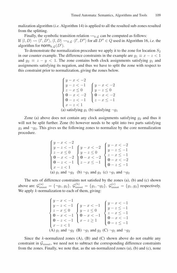
To demonstrate the normalization procedure we apply it to the zone for location S2
in our counter example. The difference constraints in the example are g1 ≡ x − z < 1and g2 ≡ z − y < 1. The zone contains both clock assignments satisfying g1 andassignments satisfying its negation, and thus we have to split the zone with respect tothis constraint prior to normalization, giving the zones below.
y − x < −2y − z < −1z − x ≤ 00− x < −20− z < −1x− z < 1
y − x < −2y − z ≤ 00− x < −2z − x ≤ −1
(a) satisfying g1 (b) satisfying ¬g1Zone (a) above does not contain any clock assignments satisfying g2 and thus it
will not be split further. Zone (b) however needs to be split into two parts satisfyingg2 and ¬g2. This gives us the following zones to normalize by the core normalizationprocedure.
y − x < −2y − z < −1z − x ≤ 00 − x < −20 − z < −1x− z < 1
y − x < −2y − z ≤ 00− x < −2z − x ≤ −1
y − x < −2y − z ≤ −1z − x ≤ −10− x < −20− z ≤ −1
(a) g1 and ¬g2 (b) ¬g1 and g2 (c) ¬g1 and ¬g2The sets of difference constraints not satisfied by the zones (a), (b) and (c) shown
above are: G(a)unsat = {¬g1, g2}, G(b)
unsat = {g1,¬g2}, G(c)unsat = {g1, g2} respectively.
We apply k-normalization to each of them, giving:
y − x < −1y − z < −1z − x ≤ 00− x < −10− z < −1x− z < 1
y − x < −1y − z ≤ 00− x < −1x− z ≥ 1
y − x < −1y − z ≤ −1z − x ≤ −10− x < −10− z ≤ −1
(A) g1 and ¬g2 (B) ¬g1 and g2 (C) ¬g1 and ¬g2Since the k-normalized zones (A), (B) and (C) shown above do not enable any
constraint in Gunsat, we need not to subtract the corresponding difference constraintsfrom the zones. Finally, we note that, as the un-normalized zones (a), (b) and (c), none
110 Johan Bengtsson and Wang Yi
of the normalized zones (A), (B) and (C) intersects with g1 ∧ g2; the transition from S2
to S3 is not enabled by the normalization procedure.
4.4 Zones in Memory
This section describes a number of techniques for storing zones in computer memory.The section starts by describing how to map DBM elements on machine words. It con-tinues by discussing how to place two-dimensional DBMs in linear memory and endsby describing how to store zones using a sparse representation.
Storing DBM Elements. To store a DBM element in memory we need to keep trackof the integer limit and whether it is strict or not. The range of the integer limit istypically much lower than the maximum value of a machine word and the strictness canbe stored using just one bit. Thus, it is possible to store both the limit and the strictness indifferent parts of the same machine word. Since comparing and adding DBM elementsare frequently used operations it is crucial for the performance of a DBM package thatthey can be efficiently implemented for the chosen encoding. Fortunately, it is possibleto construct an encoding of bounds in machine words, where checking if b1 is less thanb2 can be performed by checking if the encoded b1 is smaller than the encoded b2.
The encoding we propose is to use the least significant bit (LSB) of the machineword to store whether the bound is strict or not. Since strict bounds are smaller thannon-strict we let a set (1) bit denote that the bound is non-strict while an unset (0) bitdenote that the bound is strict. The rest of the bits in the machine word are used to storethe integer bound. To encode ∞ we use the largest positive number that fit in a machineword (denoted MAX_INT).
For good performance we also need an efficient implementation of addition ofbounds. For the proposed encoding Algorithm 17 adds two encoded bounds b1 andb2. The symbols & and | in the algorithm are used to denote bitwise-and and bitwise-or,respectively.
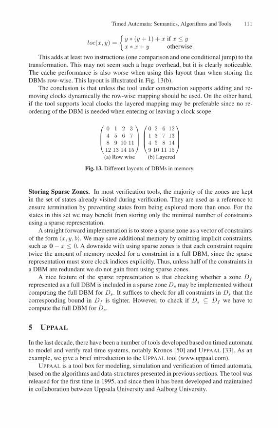
Placing DBMs in Memory. Another issue is how to store two-dimensional DBMsin linear memory. In this section we present two different techniques and give a briefcomparison between them. The natural way to put matrices in linear memory is to storethe elements by row (or by column), i.e. each row of the matrix is stored consequentlyin memory. This layout has one big advantage, its good performance. This advantage ismainly due to the simple function for computing the location of a given element in thematrix: loc(x, y) = x∗(n+1)+y. This function can (on most computers) be computedin only two instructions. This is important since all accesses to DBM elements use thisfunction. How the different DBM elements are place in memory with this layout ifpresented in Fig. 13(a).
The second way to store a DBM in linear memory is based on a layered model whereeach layer consists of the bounds between a clock and the clocks with lower index in theDBM. In this representation it is cheap to implement local clocks, since all informationabout the local clocks are localised at the end of the DBM. The drawback with thislayout is the more complicated function from DBM indices to memory locations. Forthis layout we have:
Timed Automata: Semantics, Algorithms and Tools 111
loc(x, y) ={y ∗ (y + 1) + x if x ≤ yx ∗ x+ y otherwise
This adds at least two instructions (one comparison and one conditional jump) to thetransformation. This may not seem such a huge overhead, but it is clearly noticeable.The cache performance is also worse when using this layout than when storing theDBMs row-wise. This layout is illustrated in Fig. 13(b).
The conclusion is that unless the tool under construction supports adding and re-moving clocks dynamically the row-wise mapping should be used. On the other hand,if the tool supports local clocks the layered mapping may be preferable since no re-ordering of the DBM is needed when entering or leaving a clock scope.
0 1 2 34 5 6 78 9 10 1112 13 14 15
0 2 6 121 3 7 134 5 8 149 10 11 15
(a) Row wise (b) Layered
Fig. 13. Different layouts of DBMs in memory.
Storing Sparse Zones. In most verification tools, the majority of the zones are keptin the set of states already visited during verification. They are used as a reference toensure termination by preventing states from being explored more than once. For thestates in this set we may benefit from storing only the minimal number of constraintsusing a sparse representation.
A straight forward implementation is to store a sparse zone as a vector of constraintsof the form 〈x, y, b〉. We may save additional memory by omitting implicit constraints,such as 0 − x ≤ 0. A downside with using sparse zones is that each constraint requiretwice the amount of memory needed for a constraint in a full DBM, since the sparserepresentation must store clock indices explicitly. Thus, unless half of the constraints ina DBM are redundant we do not gain from using sparse zones.
A nice feature of the sparse representation is that checking whether a zone Df
represented as a full DBM is included in a sparse zoneDs may be implemented withoutcomputing the full DBM for Ds. It suffices to check for all constraints in Ds that thecorresponding bound in Df is tighter. However, to check if Ds ⊆ Df we have tocompute the full DBM for Ds.
5 UPPAAL
In the last decade, there have been a number of tools developed based on timed automatato model and verify real time systems, notably Kronos [50] and UPPAAL [33]. As anexample, we give a brief introduction to the UPPAAL tool (www.uppaal.com).
UPPAAL is a tool box for modeling, simulation and verification of timed automata,based on the algorithms and data-structures presented in previous sections. The tool wasreleased for the first time in 1995, and since then it has been developed and maintainedin collaboration between Uppsala University and Aalborg University.
112 Johan Bengtsson and Wang Yi
5.1 Modeling with UPPAAL
The core of the UPPAAL modeling language is networks of timed automata. In addition,the language has been further extended with features to ease the modeling task and toguide the verifier in state space exploration. The most important of these are sharedinteger variables, urgent channels and committed locations.
Networks of Timed Automata. A network of timed automata is the parallel compo-sition A1| · · · |An of a set of timed automata A1, . . . , An, called processes, combinedinto a single system by the CCS parallel composition operator with all external actionshidden. Synchronous communication between the processes is by hand-shake synchro-nization using input and output actions; asynchronous communication is by shared vari-ables as described later. To model hand-shake synchronization, the action alphabetΣ isassumed to consist of symbols for input actions denoted a?, output actions denoted a!,and internal actions represented by the distinct symbol τ .
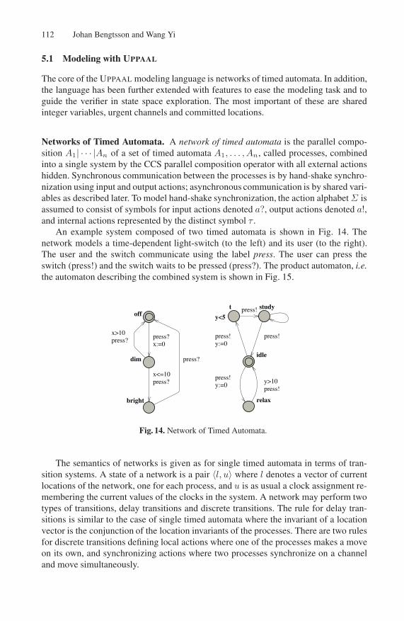
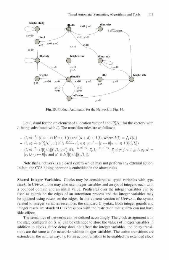
An example system composed of two timed automata is shown in Fig. 14. Thenetwork models a time-dependent light-switch (to the left) and its user (to the right).The user and the switch communicate using the label press. The user can press theswitch (press!) and the switch waits to be pressed (press?). The product automaton, i.e.the automaton describing the combined system is shown in Fig. 15.
off
dim
bright
press?x:=0
x<=10press?
x>10press?
press?
t
y<5
study
idle
relax
press!y:=0
press!y>10
press!y:=0
press!
press!
Fig. 14. Network of Timed Automata.
The semantics of networks is given as for single timed automata in terms of tran-sition systems. A state of a network is a pair 〈l, u〉 where l denotes a vector of currentlocations of the network, one for each process, and u is as usual a clock assignment re-membering the current values of the clocks in the system. A network may perform twotypes of transitions, delay transitions and discrete transitions. The rule for delay tran-sitions is similar to the case of single timed automata where the invariant of a locationvector is the conjunction of the location invariants of the processes. There are two rulesfor discrete transitions defining local actions where one of the processes makes a moveon its own, and synchronizing actions where two processes synchronize on a channeland move simultaneously.
Timed Automata: Semantics, Algorithms and Tools 113
off,idle dim,relax
dim,t
y<5
bright, study
off,study
bright,t
y<5
dim,idle
bright,relax dim,study
off,t
y<5
bright, idle
off,relax
x:=0, y:=0
x>10, y>10
x:=0, y:=0
x<=10
x>10
x:=0
x<=10 y:=0
x<10y:=0
x>10
x>10 y:=0
x>10
x<=10,y>10
x<=10
y:=0
x>10y:=0
y>10x:=0
y:=0
Fig. 15. Product Automaton for the Network in Fig. 14.
Let li stand for the ith element of a location vector l and l[l′i/li] for the vector l withli being substituted with l′i. The transition rules are as follows:
– 〈l, u〉 d−→ 〈l, u+ t〉 if u ∈ I(l) and (u+ d) ∈ I(l), where I(l) =∧I(li)
– 〈l, u〉 τ−→ 〈l[l′i/li], u′〉 if lig,τ,r−−−→ l′i, u ∈ g, u′ = [r → 0]u, u′ ∈ I(l[l′i/li])
– 〈l, u〉 τ−→ ⟨l[l′i/li][l
′j/lj], u
′⟩ if ligi,a?,ri−−−−−→ l′i, lj
gj ,a!,rj−−−−−→ l′j , i �= j, u ∈ gi ∧ gj , u′ =
[ri ∪ rj → 0]u and u′ ∈ I(l[l′i/li][l′j/lj]).
Note that a network is a closed system which may not perform any external action.In fact, the CCS hiding operator is embedded in the above rules.
Shared Integer Variables. Clocks may be considered as typed variables with typeclock. In UPPAAL, one may also use integer variables and arrays of integers, each witha bounded domain and an initial value. Predicates over the integer variables can beused as guards on the edges of an automaton process and the integer variables maybe updated using resets on the edges. In the current version of UPPAAL, the syntaxrelated to integer variables resembles the standard C syntax. Both integer guards andinteger resets are standard C expressions with the restriction that guards can not haveside-effects.
The semantics of networks can be defined accordingly. The clock assignment u inthe state configuration 〈l, u〉 can be extended to store the values of integer variables inaddition to clocks. Since delay does not affect the integer variables, the delay transi-tions are the same as for networks without integer variables. The action transitions areextended in the natural way, i.e. for an action transition to be enabled the extended clock
114 Johan Bengtsson and Wang Yi
assignment must also satisfy all integer guards on the corresponding edges and when atransition is taken the assignment is updated according to the integer and clock resets.
There is a problem with variable updating in a synchronizing transition where oneof the processes participating in the transition updates a variable used by the other.In UPPAAL, for a synchronization transition, the resets on the edge with an output-label is performed before the resets on the edge with an input-label. This destroys thesymmetry of input and output actions. But it gives a natural and clear semantics forvariable updating. The transition rule for synchronization is modified accordingly:
– 〈l, u〉 τ−→ ⟨l[l′i/li][l
′j/lj], u
′⟩ if ligi,a?,ri−−−−−→ l′i, lj
gj ,a!,rj−−−−−→ l′j , i �= j, u ∈ gi ∧ gj , u′ =
[ri → 0]([rj → 0]u) and u′ ∈ I(l[l′i/li][l′j/lj])
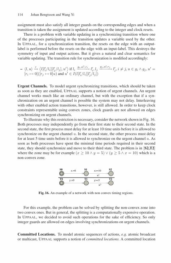
Urgent Channels. To model urgent synchronizing transitions, which should be takenas soon as they are enabled, UPPAAL supports a notion of urgent channels. An urgentchannel works much like an ordinary channel, but with the exception that if a syn-chronization on an urgent channel is possible the system may not delay. Interleavingwith other enabled action transitions, however, is still allowed. In order to keep clockconstraints representable using convex zones, clock guards are not allowed on edgessynchronizing on urgent channels.
To illustrate why this restriction is necessary, consider the network shown in Fig. 16.Both processes may independently go from their first state to their second state. In thesecond state, the first process must delay for at least 10 time units before it is allowed tosynchronize on the urgent channel u. In the second state, the other process must delayfor at least 5 time units before it is allowed to synchronize on the urgent channel u. Assoon as both processes have spent the minimal time periods required in their secondstate, they should synchronize and move to their third state. The problem is in [S2,T2]where the zone may be for example (x ≥ 10 ∧ y = 5) ∨ (y ≥ 5 ∧ x = 10) which is anon-convex zone.
S2S1S0 x:=0 x>=10
u!
T2T1T0 y:=0 y>=5
u?
Fig. 16. An example of a network with non convex timing regions.
For this example, the problem can be solved by splitting the non-convex zone intotwo convex ones. But in general, the splitting is a computationally expensive operation.In UPPAAL, we decided to avoid such operations for the sake of efficiency. So onlyinteger guards are allowed on edges involving synchronizations on urgent channels.
Committed Locations. To model atomic sequences of actions, e.g. atomic broadcastor multicast, UPPAAL supports a notion of committed locations. A committed location
Timed Automata: Semantics, Algorithms and Tools 115
is a location where no delay is allowed. In a network, if any process is in a committedlocation then only action transitions starting from such a committed location are al-lowed. Thus, processes in committed locations may be interleaved only with processesin a committed location.
Syntactically, each process Ai in a network may have a subset NCi ⊆ Ni of loca-
tions marked as committed locations. Let C(l) denote the set of locations in l, that arecommitted. For the same reason as in the case of urgent channels, as a syntactical re-striction, no clock constraints but predicates over integer variables are allowed to appearin a guard on an outgoing edge from a committed location.
The transition rules are given in the following, where →c denotes the transitionrelation for a network with committed locations and → denotes the transition relationfor the same network without considering the committed locations.
– 〈l, u〉 d−→c 〈l, u+ d〉 if 〈l, u〉 d−→ 〈l, u+ d〉 and C(l) = ∅– 〈l, u〉 τ−→c 〈l[l′i/li], u′〉 if 〈l, u〉 τ−→ 〈l[l′i/li], u′〉 and either li ∈ C(l) or C(l) = ∅– 〈l, u〉 τ−→c
⟨l[l′i/li][l
′j/lj], u
′⟩ if 〈l, u〉 τ−→ ⟨l[l′i/li][l
′j/lj], u
′⟩ and either li ∈ C(l),lj ∈ C(l) or C(l) = ∅
5.2 Verifying with UPPAAL
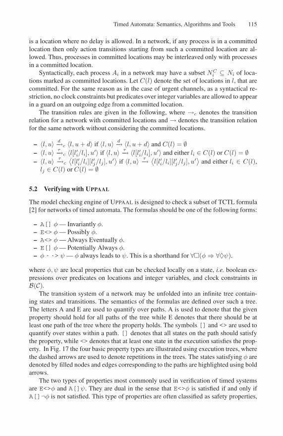
The model checking engine of UPPAAL is designed to check a subset of TCTL formula[2] for networks of timed automata. The formulas should be one of the following forms:
– A[] φ — Invariantly φ.– E<> φ — Possibly φ.– A<> φ — Always Eventually φ.– E[] φ — Potentially Always φ.– φ --> ψ — φ always leads to ψ. This is a shorthand for ∀�(φ⇒ ∀♦ψ).
where φ, ψ are local properties that can be checked locally on a state, i.e. boolean ex-pressions over predicates on locations and integer variables, and clock constraints inB(C).
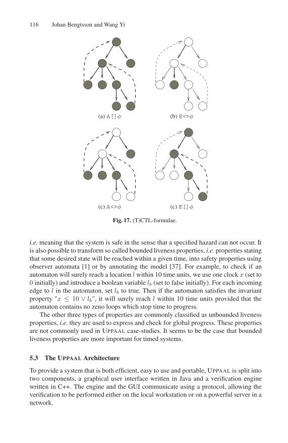
The transition system of a network may be unfolded into an infinite tree contain-ing states and transitions. The semantics of the formulas are defined over such a tree.The letters A and E are used to quantify over paths. A is used to denote that the givenproperty should hold for all paths of the tree while E denotes that there should be atleast one path of the tree where the property holds. The symbols [] and <> are used toquantify over states within a path. [] denotes that all states on the path should satisfythe property, while <> denotes that at least one state in the execution satisfies the prop-erty. In Fig. 17 the four basic property types are illustrated using execution trees, wherethe dashed arrows are used to denote repetitions in the trees. The states satisfying φ aredenoted by filled nodes and edges corresponding to the paths are highlighted using boldarrows.
The two types of properties most commonly used in verification of timed systemsare E<>φ and A[]ψ. They are dual in the sense that E<>φ is satisfied if and only ifA[]¬φ is not satisfied. This type of properties are often classified as safety properties,
116 Johan Bengtsson and Wang Yi
(a) A[]φ (b) E<>φ
(c) A<>φ (c) E[]φ
Fig. 17. (T)CTL-formulae.
i.e. meaning that the system is safe in the sense that a specified hazard can not occur. Itis also possible to transform so called bounded liveness properties, i.e. properties statingthat some desired state will be reached within a given time, into safety properties usingobserver automata [1] or by annotating the model [37]. For example, to check if anautomaton will surely reach a location l within 10 time units, we use one clock x (set to0 initially) and introduce a boolean variable lb (set to false initially). For each incomingedge to l in the automaton, set lb to true. Then if the automaton satisfies the invariantproperty "x ≤ 10 ∨ lb", it will surely reach l within 10 time units provided that theautomaton contains no zeno loops which stop time to progress.
The other three types of properties are commonly classified as unbounded livenessproperties, i.e. they are used to express and check for global progress. These propertiesare not commonly used in UPPAAL case-studies. It seems to be the case that boundedliveness properties are more important for timed systems.
5.3 The UPPAAL Architecture
To provide a system that is both efficient, easy to use and portable, UPPAAL is split intotwo components, a graphical user interface written in Java and a verification enginewritten in C++. The engine and the GUI communicate using a protocol, allowing theverification to be performed either on the local workstation or on a powerful server in anetwork.
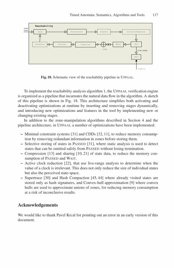
Timed Automata: Semantics, Algorithms and Tools 117
Fig. 18. Schematic view of the reachability pipeline in UPPAAL.
To implement the reachability analysis algorithm 1, the UPPAAL verification engineis organized as a pipeline that incarnates the natural data flow in the algorithm. A sketchof this pipeline is shown in Fig. 18. This architecture simplifies both activating anddeactivating optimizations at runtime by inserting and removing stages dynamically,and introducing new optimizations and features in the tool by implementing new orchanging existing stages.
In addition to the zone-manipulation algorithms described in Section 4 and thepipeline architecture, in UPPAAL a number of optimizations have been implemented:
– Minimal constraint systems [31] and CDDs [32, 11], to reduce memory consump-tion by removing redundant information in zones before storing them.
– Selective storing of states in PASSED [31], where static analysis is used to detectstates that can be omitted safely from PASSED without losing termination.
– Compression [13] and sharing [10, 21] of state data, to reduce the memory con-sumption of PASSED and WAIT.
– Active clock reduction [22], that use live-range analysis to determine when thevalue of a clock is irrelevant. This does not only reduce the size of individual statesbut also the perceived state-space.
– Supertrace [30] and Hash Compaction [45, 44] where already visited states arestored only as hash signatures, and Convex-hull approximation [9] where convexhulls are used to approximate unions of zones, for reducing memory consumptionat a risk of inconclusive results.
Acknowledgements
We would like to thank Pavel Krcal for pointing out an error in an early version of thisdocument.
118 Johan Bengtsson and Wang Yi
Appendix: Pseudo-Code for Operations on DBMs
Algorithm 2 close(D): Floyds algorithm for computing shortest path
for k := 0 to n dofor i := 0 to n do
for j := 0 to n doDij := min(Dij , Dik + Dkj)
end forend for
end for
Algorithm 3 Reduction of Zero-Cycle Free Graph G with n nodes
for i := 1 to n dofor j := 1 to n do
for k := 1 to n doif Gik + Gkj ≤ Gij then
Mark edge i → j as redundantend if
end forend for
end forRemove all edges marked as redundant.
Algorithm 4 Reduction of negative-cycle free graph G with n nodes
for i := 1 to n doif Nodei is not in a partition then
Eqi = ∅for j := i to n do
if Gij + Gji = 0 thenEqi := Eqi ∪ {Nodei}
end ifend for
end ifend forLet G′ be a graph without nodes.for each Eqi do
Pick one representative Nodei ∈ Eqi
Add Nodei to G′
Connect Nodei to all nodes in G′ using weights from G.end forReduce G′
for each Eqi doAdd one zero cycle containing all nodes in Eqi to G′
end for
Timed Automata: Semantics, Algorithms and Tools 119
Algorithm 5 relation(D,D′)
fD⊆D′ := ttfD⊇D′ := ttfor i := 0 to n do
for j := 0 to n dofD⊆D′ := fD⊆D′ ∧ (Dij ≤ D′
ij)fD⊇D′ := fD⊇D′ ∧ (Dij ≥ D′
ij)end for
end forreturn 〈fD⊆D′ , fD⊇D′〉
Algorithm 6 up(D)
for i := 1 to n doDi0 := ∞
end for
Algorithm 7 down(D)
for i := 1 to n doD0i = (0,≤)for j := 1 to n do
if Dji < D0i thenD0i = Dji
end ifend for
end for
Algorithm 8 and(D, g)
if Dyx + (m,�) < 0 thenD00 = (−1,≤)
else if (m,�) < Dxy thenDxy = (m,�)for i := 0 to n do
for j := 0 to n doif Dix + Dxj < Dij then
Dij = Dix + Dxj
end ifif Diy + Dyj < Dij then
Dij = Diy + Dyj
end ifend for
end forend if
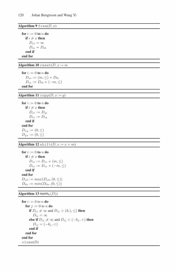
120 Johan Bengtsson and Wang Yi
Algorithm 9 free(D, x)
for i := 0 to n doif i �= x then
Dxi = ∞Dix = Di0
end ifend for
Algorithm 10 reset(D, x := m
for i := 0 to n doDxi := (m,≤) + D0i
Dix := Di0 + (−m,≤)end for
Algorithm 11 copy(D, x := y)
for i := 0 to n doif i �= x then
Dxi := Dyi
Dix := Diy
end ifend forDxy := (0,≤)Dyx := (0,≤)
Algorithm 12 shift(D, x := x + m)
for i := 0 to n doif i �= x then
Dxi := Dxi + (m,≤)Dix := Dix + (−m,≤)
end ifend forDx0 := max(Dx0, (0,≤))D0x := min(D0x, (0,≤))
Algorithm 13 normk(D))
for i := 0 to n dofor j := 0 to n do
if Dij �= ∞ and Dij > (ki),≤) thenDij = ∞
else if Dij �= ∞ and Dij < (−kj , <) thenDij = (−kj , <)
end ifend for
end forclose(D)
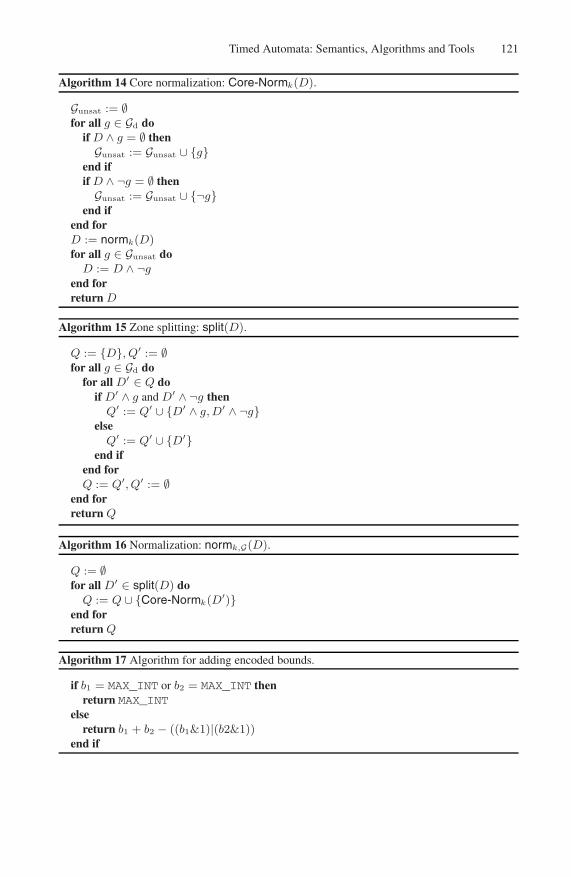
Timed Automata: Semantics, Algorithms and Tools 121
Algorithm 14 Core normalization: Core-Normk(D).
Gunsat := ∅for all g ∈ Gd do
if D ∧ g = ∅ thenGunsat := Gunsat ∪ {g}
end ifif D ∧ ¬g = ∅ thenGunsat := Gunsat ∪ {¬g}
end ifend forD := normk(D)for all g ∈ Gunsat do
D := D ∧ ¬gend forreturn D
Algorithm 15 Zone splitting: split(D).
Q := {D}, Q′ := ∅for all g ∈ Gd do
for all D′ ∈ Q doif D′ ∧ g and D′ ∧ ¬g then
Q′ := Q′ ∪ {D′ ∧ g, D′ ∧ ¬g}else
Q′ := Q′ ∪ {D′}end if
end forQ := Q′, Q′ := ∅
end forreturn Q
Algorithm 16 Normalization: normk,G(D).
Q := ∅for all D′ ∈ split(D) do
Q := Q ∪ {Core-Normk(D′)}end forreturn Q
Algorithm 17 Algorithm for adding encoded bounds.
if b1 = MAX_INT or b2 = MAX_INT thenreturn MAX_INT
elsereturn b1 + b2 − ((b1&1)|(b2&1))
end if
122 Johan Bengtsson and Wang Yi
References
1. Luca Aceto, Augusto Bergueno, and Kim G. Larsen. Model checking via reachability test-ing for timed automata. In Proceedings, Fourth Workshop on Tools and Algorithms for theConstruction and Analysis of Systems, volume 1384 of Lecture Notes in Computer Science.Springer-Verlag, 1998.
2. Rajeev Alur, Costas Courcoubetis, and David L. Dill. Model-checking for real-time systems.In Proceedings, Seventh Annual IEEE Symposium on Logic in Computer Science, pages414–425. IEEE Computer Society Press, 1990.
3. Rajeev Alur, Costas Courcoubetis, and David L. Dill. Model-checking in dense real-time.Journal of Information and Computation, 104(1):2–34, 1993.
4. Rajeev Alur, Costas Courcoubetis, and Thomas A. Henzinger. The observational power ofclocks. In International Conference on Concurrency Theory, pages 162–177, 1994.
5. Rajeev Alur and David L. Dill. Automata for modeling real-time systems. In Proceedings,Seventeenth International Colloquium on Automata, Languages and Programming, volume443 of Lecture Notes in Computer Science, pages 322–335. Springer-Verlag, 1990.
6. Rajeev Alur and David L. Dill. A theory of timed automata. Journal of Theoretical ComputerScience, 126(2):183–235, 1994.
7. Rajeev Alur, Limor Fix, and Thomas A. Henzinger. Event-clock automata: a determinizableclass of timed automata. Theoretical Computer Science, 211(1–2):253–273, 1999.
8. Rajeev Alur and Thomas A. Henzinger. A really temporal logic. Journal of the ACM,41(1):181–204, 1994.
9. Felice Balarin. Approximate reachability analysis of timed automata. In Proceedings, 17thIEEE Real-Time Systems Symposium. IEEE Computer Society Press, 1996.
10. Gerd Behrmann, Alexandre David, Kim G. Larsen, and Wang Yi. Unification & sharing intimed automata verification. In Proceedings, Tenth International SPIN Workshop, volume2648 of Lecture Notes in Computer Science. Springer-Verlag, 2003.
11. Gerd Behrmann, Kim G. Larsen, Justin Pearson, Carsten Weise, and Wang Yi. Efficient timedreachability analysis using clock difference diagrams. In Proceedings, Eleventh InternationalConference on Computer Aided Verification, volume 1633 of Lecture Notes in ComputerScience, pages 341–353. Springer-Verlag, 1999.
12. Richard Bellman. Dynamic Programming. Princeton University Press, 1957.13. Johan Bengtsson. Reducing memory usage in symbolic state-space exploration for timed
systems. Technical Report 2001-009, Department of Information Technology, Uppsala Uni-versity, 2001.
14. Johan Bengtsson. Clocks, dbms and states in timed systems. Ph.D. Thesis, ACTA Universi-tatis Upsaliensis 39, Uppsala University, 2002.
15. Johan Bengtsson, Bengt Jonsson, Johan Lilius, and Wang Yi. Partial order reductions fortimed systems. In Proceedings, Ninth International Conference on Concurrency Theory, vol-ume 1466 of Lecture Notes in Computer Science, pages 485–500. Springer-Verlag, 1998.
16. Johan Bentsson and Wang Yi. On clock difference constraints and termination in reachabilityanalysis of timed automata. In Formal Methods and Software Engineering, 5th InternationalConference on Formal Engineering Methods, ICFEM 2003, Singapore, November 5-7, 2003,Proceedings, volume 2885 of Lecture Notes in Computer Science. Springer, 2003.
17. Bernard Berthomieu and Michel Diaz. Modeling and verification of timed dependent systemsusing timed petri nets. IEEE Transactions on Software Engineering, 17(3):259–273, 1991.
18. Beatrice Bérard, Volker Diekert, Paul Gastin, and Antoine Petit. Characterization of the ex-pressive power of silent transitions in timed automata. Fundamenta Informaticae, 36:145–182, 1998.
Timed Automata: Semantics, Algorithms and Tools 123
19. Karlis Cerans. Decidability of bisimulation equivalences for parallel timer processes. InComputer Aided Verification, volume 663 of LNCS. Springer, 1992.
20. Zhou Chaochen. Duration calculus, a logical approach to real-time systems. Lecture Notesin Computer Science, 1548:1–7, 1999.
21. Alexandre David, Gerd Behrmann, Kim G. Larsen, and Wang Yi. A tool architecture for thenext genreation of UPPAAL. Technical Report 2003-011, Department of Information Tech-nology, Uppsala University, 2003.
22. Conrado Daws and Sergio Yovine. Reducing the number of clock variables of timed au-tomata. In Proceedings, 17th IEEE Real-Time Systems Symposium. IEEE Computer SocietyPress, 1996.
23. David L. Dill. Timing assumptions and verification of finite-state concurrent systems. InProceedings, Automatic Verification Methods for Finite State Systems, volume 407 of LectureNotes in Computer Science, pages 197–212. Springer-Verlag, 1989.
24. Elena Fersman, Paul Pettersson, and Wang Yi. Timed automata with asynchronous processes:Schedulability and decidability. In J.-P. Katoen and P. Stevens, editors, Proc. of the 8th Inter-national Conference on Tools and Algorithms for the Construction and Analysis of Systems,number 2280 in Lecture Notes in Computer Science, pages 67–82. Springer–Verlag, 2002.
25. Robert W. Floyd. Acm algorithm 97: Shortest path. Communications of the ACM, 5(6):345,June 1962.
26. N. Halbwachs. Delay analysis in synchronous programs. In Fifth Conference on Computer-Aided Verification, Elounda (Greece), July 1993. LNCS 697, Springer Verlag.
27. Thomas A. Henzinger, Xavier Nicollin, Joseph Sifakis, and Sergio Yovine. Symbolic modelchecking for real-time systems. In Proceedings, Seventh Annual IEEE Symposium on Logicin Computer Science, pages 394–406, 1992.
28. Thomas A. Henzinger, Xavier Nicollin, Joseph Sifakis, and Sergio Yovine. Symbolic modelchecking for real-time systems. Journal of Information and Computation, 111(2):193–244,1994.
29. C.A.R. Hoare. Communicating sequential processes. Communications of the ACM,21(8):666–676, August 1978.
30. Gerard J. Holzmann. Design and Validation of Computer Protocols. Prentice-Hall, 1991.31. Kim G. Larsen, Fredrik Larsson, Paul Pettersson, and Wang Yi. Efficient verification of real-
time systems: Compact data structure and state space reduction. In Proceedings, 18th IEEEReal-Time Systems Symposium, pages 14–24. IEEE Computer Society Press, 1997.
32. Kim G. Larsen, Justin Pearson, Carsten Weise, and Wang Yi. Clock difference diagrams.Nordic Journal of Computing, 1999.
33. Kim G. Larsen, Paul Petterson, and Wang Yi. UPPAAL in a nutshell. Journal on SoftwareTools for Technology Transfer, 1997.
34. Kim G. Larsen, Paul Pettersson, and Wang Yi. Compositional and Symbolic Model-Checking of Real-Time Systems. In Proc. of the 16th IEEE Real-Time Systems Symposium,pages 76–87. IEEE Computer Society Press, December 1995.
35. Kim Guldstrand Larsen and Yi Wang. Time-abstracted bisimulation: Implicit specificationsand decidability. Information and Computation, 134(2):75–101, 1997.
36. Fredrik Larsson. Efficient implementation of model-checkers for networks of timed au-tomata. Licentiate Thesis 2000-003, Department of Information Technology, Uppsala Uni-versity, 2000.
37. Magnus Lindahl, Paul Pettersson, and Wang Yi. Formal Design and Analysis of a Gear-BoxController. In Proceedings, Fourth Workshop on Tools and Algorithms for the Constructionand Analysis of Systems, number 1384 in Lecture Notes in Computer Science, pages 281–297. Springer-Verlag, 1998.
124 Johan Bengtsson and Wang Yi
38. Magnus Lindahl, Paul Pettersson, and Wang Yi. Formal Design and Analysis of a GearboxController. Springer International Journal of Software Tools for Technology Transfer (STTT),3(3):353–368, 2001.
39. Robin Milner. Communication and Concurrency. Prentice Hall, 1989.40. Xavier Nicollin and Joseph Sifakis. The algebra of timed processes, ATP: Theory and appli-
cation. Journal of Information and Computation, 114(1):131–178, 1994.41. Paul Pettersson. Modelling and Verification of Real-Time Systems Using Timed Automata:
Theory and Practice. PhD thesis, Uppsala University, 1999.42. G. M. Reed and A. W. Roscoe. A timed model for communicating sequential processes.
Theoretical Computer Science, 58(1-3):249–261, 1988.43. Tomas Gerhard Rokicki. Representing and Modeling Digital Circuits. PhD thesis, Stanford
University, 1993.44. Ulrich Stern and David L. Dill. Improved probabilistic verification by hash compaction.
In Correct Hardware Design and Verification Methods: IFIP WG10.5 Advanced ResearchWorking Conference Proceedings, 1995.
45. Pierre Wolper and Dennis Leroy. Reliable hashing without collision detection. In Proceed-ings, Fifth International Conference on Computer Aided Verification, volume 697 of LectureNotes in Computer Science, pages 59–70. Springer-Verlag, 1993.
46. Mihalis Yannakakis and David Lee. An efficient algorithm for minimizing real-time transi-tion systems. In Proceedings, Fifth International Conference on Computer Aided Verifica-tion, volume 697 of Lecture Notes in Computer Science, pages 210–224. Springer-Verlag,1993.
47. Wang Yi. CCS + time = an interleaving model for real time systems. In Proceedings, Eigh-teenth International Colloquium on Automata, Languages and Programming, volume 510 ofLecture Notes in Computer Science. Springer-Verlag, 1991.
48. Wang Yi and B. Jonsson. Decidability of timed language-inclusion for networks of real-time communicating sequen tial processes. In Proc. 14th Conf. on Foundations of SoftwareTechnology and Theoretical Computer Science, volume 880 of Lecture Notes in ComputerScience. Springer-Verlag, 1994.
49. Wang Yi, Paul Petterson, and Mats Daniels. Automatic verification of real-time communi-cating systems by constraint-solving. In Proceedings, Seventh International Conference onFormal Description Techniques, pages 223–238, 1994.
50. Sergio Yovine. Kronos: a verification tool for real-time systems. Journal on Software Toolsfor Technology Transfer, 1, October 1997.


![LSVbouyer/files/bouyer-hdr-soutenance.pdf · Reachability analysis in timed automata Improving further [BBFL03] Behrmann, Bouyer, Fleury, Larsen. Static Guard Analysis in Timed Automata](https://img.pdfslide.us/doc/110x75/603cf1d0e6e2e567542a1a08/bouyerfilesbouyer-hdr-soutenancepdf-reachability-analysis-in-timed-automata.jpg)