EE296B Luke Snow Project Due: Thurs. 12/10/09

Channel Analysis Using USRP

I. Introduction

An important part of communications links is the channel. With knowledge of the channel, one can

build filters to cancel the effects of the channel, thereby more faithfully reproducing the message sent. Thus the actual measuring of the channel is necessary.

This report gives the results and analysis of an indoor channel measurement. The Universal Software Radio Peripheral (USRP) boards, in conjunction with the GUI GnuRadio Companion (GRC) are used

as the transmitter and receiver for a spread spectrum sliding correlator channel sounding setup. Some of the relevant parameters describing the channel are also found herein.

II. Theory

A spread spectrum correlator is implemented by sending a Pseudo-random Number sequency (PN sequence) from the transmitter to the receivers. First, it is helpful to review some of the basic

properties of the PN sequence. A PN sequence is a list of 1's and -1's in a chain. The sequence is not truly random; it is generated, for

example, by a Galois Linear Feedback Shift Register (GLFSR). The sequence has a maximum length𝐿 = 2𝑁 −1, known as the "chip length", after which it repeats. The chip rate,𝑇𝑐is the rate at

which each sample (a 1 or -1) is sent. In this setup, it is the sampling frequency. Since the sequence

should simulate a random signal, it should have a broad, flat spectrum, similar to noise. The perhaps the most important property of a PN sequence is that its autocorrelation function is

"peaky" – that is, it is like a delta function. The autocorrelation of the PN sequence is given by

𝑅𝑐(𝜏) = 1–𝐿+1

𝐿𝑇𝑐[𝑢(𝜏 + 𝑇𝑐)–𝑢(𝜏– 𝑇𝑐)]−

1

𝐿[𝑢(𝜏 − 𝑇𝑐)+ 𝑢(−𝜏 − 𝑇𝑐)](1).

For large L and small𝑇𝑐the 1/L term becomes negligible and the width of the peak becomes small, so

that the autocorrelation approximates a kronecker delta function.

This is useful for channel measurement, as shown by the following argument. Suppose a PN sequence, s(t), is transmitted through the channel h(t). The received signal is then r(t) = s(t)*h(t). The receiver

has the same PN sequence, and autocorrelates the received signal with its own copy of the PN sequence. Thus

𝑟(𝑡) ∗ 𝑠(−𝑡) = 𝑠(𝑡) ∗ ℎ(𝑡) ∗ 𝑠(−𝑡) = 𝑅𝑐(𝑡) ∗ ℎ(𝑡) ≈ 𝛿(𝑡) ∗ ℎ(𝑡) = ℎ(𝑡)(2)

This means that if we transmit a PN sequence, and then correlate the sequence with itself at the receiver, we obtain a channel estimate.

III. Experimental, Results and Discussion

a. PN sequence verification. The channel sounder was implemented as given in figs. 1 and 2. The various parameters of the sounder are given in table 1.

Figure 1 – channel sounder, TX.

Figure 2 – channel sounder, RX.

Frequency 900MHz

PN sequence Chip rate 32 K chips/s; 32 M chips/s;

PN sequence Length (L) 63 chips; 4095 chips;

Resolution 31.25𝜇𝑠; 31.25𝑛𝑠;

Maximum delay observable 2ms;128𝜇𝑠;

GLFSR settings - Degree 6; 12;

- Mask 0; 0;

- Seed 4; 0;

Tx Interpolation 400

Rx Decimation 200

Tx gain 100 dB; 100 dB; (20 dB + mult. signal by 10K)

Rx gain 0 dB; 20 dB;

Table 1 – The specifications of the channel sounder. (GLFSR, sample rate, etc.) Second value is the synced clocks trial.

Before actually sending a PN sequence, it is important to verify that the output of the GLFSR block actually has the properties of a PN sequence. Recall that the sequence should appear random, and it should also have a flat spectrum. To verify the properties of the PN sequence, the setup of figs. 3 and 4, below, are used.

Figure 3 – Block diagram of the PN sequence measuring the spectrum of the signal.

Figure 4 – Block diagram of a PN sequence Transmitted through no channel, and correlated with itself.

The FFT plot of the PN sequence specified is given in fig. 5.

Figure 5 – FFT plot of the PN sequence spectrum. The important feature of the FFT plot is that the sequence has components spread across the whole

spectrum. The sequence appeared random in the time domain, since the scope trigger couldn't lock onto any repeated features of the sequence.

When using the setup of fig. 4, the plot of the autocorrelation function for this PN sequence is given in fig. 6, below.

The plots of figs. 5a and 5b give the spectrum and scope plot of the autocorrelation for the PN sequence

with degree 12, mask 0, and seed 4. This corresponds to a PN sequence of length 4095. Note that the spectrum looks more akin to that of noise, and is also spread over the whole 16MHz of bandwidth. The plot of fig. 5c gives the autocorrelation for the length 4095 PN sequence.

Figure 5a – The spectrum of a PN sequence of length 4095.

Figure 5b – The time domain plot of a PN sequence of length 4095.

Figure 5c – The autocorrelation of the length 4095 PN sequence.

Figure 6 – The PN sequence autocorrelation. This is exactly the form predicted by equation (1) above. Notice that the amplitude is nearly 1, as

required for a kronecker delta function, and the amplitude of the function away from the peak is just below zero, or−1 𝐿⁄ = 1 63⁄ ≈ −0.015.

As another test, the block diagram of fig. 7 was used. A channel with multipath components was

simulated by adding delays, plus the LOS. The output is given in fig. 8.

Figure 7 – Simulating a multipath channel.

Figure 8 – The Results of the simulation.

The LOS component is mixed with the delay of 1 sample to form a rectangular pulse type of shape, while the next multipaths correspond to the triangular pulses of 3, 10, and 30 samples. As will be seen later, the resolution of the experiment is such that all of the multipaths from the indoor environment will be grouped with the LOS. b. Layout of the room in which the experiments were carried out. Multiple experiments were carried out within the communications lab, in eng 238. The transmitter was positioned at lab station 1, on top of the 'scopes on the elevated center divide of the table. The receiver was then placed at stations 2-4, in one of two positions: on top of the 'scopes on the center divide (as for the transmitter) – Line of Sight (LOS) – or behind the 'scopes on the side of the table further from the transmitter – No Line of Sight (NLOS). A diagram of this setup is shown in fig. 9. In fig. 9, the position on top of the scopes in the center divide is labeled 'a' for the receiver positions, and 'Tx' for the transmitter position. The position behind the oscilloscopes, on the further side of the table, is labeled 'b'.

When positioned at 'a' of each station, the receiver and transmitter antennae were coplanar and paralllel. Thus the dominant effect, with LOS, should be path loss. When positioned at 'b' of each station, the antennae were parallel, but not coplanar. The height from position 'b' to the level of position 'a' is approximately 53cm. The distance, in the plane of the diagram, between 'a' and 'b' was approximately 23cm. There was also a trial with the USRPs having synchronized clocks; this trial was done on a cart half way between stations 1 and 2, with the boards less than a meter apart from eachother, with LOS, using both desktop computers. This is trial 2s. An experiment was also done with a moving receiver; this is trial 2m.

| | |

Figure 9 – A diagram of the room, and the positioning of stations 1-4.

The various distances between the receiver and transmitter antennae are shown in table 2.

Station Distance between Tx and Rx. (cm)

2a 284

2b 312

2s* < 50

2m <300

3a 511

4a 845

4b 855

4d* 845

a b

a a

Tx

b b

1

3 2 4

284cm

425cm 371cm

Table 2 – The distances between the Tx and Rx antennae at the various stations. *The data of 4d was taken at a sampling frequency of 4MHz. The data of 2s was taken at a sampling frequency of 32MHz.

c. Station 2 trials Initially, the data comes in two dimensions: one is counts, the other samples; however, since the PN sequence data repeats itself, the received signal can be chopped into plots of length 63, and then all placed next to eachother, to form the Channel Impulse Response (CIR). The first period of the trial 2a data is given in fig. 10. A centered view of the second peak, and its autocorrelation, are given in figs. 11 and 12, respectively.

From fig. 12 (autocorr), the width of the autocorrelation is about 66 samples, or 2.06 ms. This corresponds to

the RMS delay spread. Taking the coherence bandwidth as 𝐵𝑐 ≈1

50𝜎𝜏, a value of about 9.7 Hz. Since the signal

has a larger bandwidth than this, the system has frequency selective fading. Also of interest is the width of the LOS peak in figs. 10 and 11. One would expect a peak width of 2 samples for a single LOS, but the peak width was 6 samples, or 187.5us. This is due to the short timescale multipaths, all piled into the LOS bin.

Figure 10 – The first period of the PN sequence of trial 2a.

Figure 11 – A centered view of the LOS for the second peak of trial 2a.

Figure 12 – The autocorrelation. The CIR and Power Delay Profile (DP) for the receiver position at stations 2a and 2b are given in figs. 13 – 16. No distinct multipath components are visible. This would make sense, since the multipaths within a room are on the order of nanoseconds, while the resolution of the experiment, with a sampling frequency of 32KHz, is 31.25 us. Thus the multipaths are all grouped within the LOS peak, clearly indicated in the below plots. Interestingly, one would expect all of the LOS peaks to have a constant delay. However, as is evident from the

plots, the LOS peaks have a peak that gradually shifts up the delay as time goes on. This appears to be due to the lack of synchronization between the Tx and Rx clocks.

Figure 13 – The CIR for the data taken with the receiver at position 2a.

Figure 14 – The DP for the data taken with the receiver at position 2a.

Figure 15 – The CIR for the data taken with the receiver at position 2b.

Figure 16 – The DP for the data taken with the receiver at position 2b.

The data in table 3 gives the delay and time indices of some of the LOS peaks fig. 13.

X, or

Tau

Y, or

time

4 121

6 390

9 822

13 1345

21 2452

24 2836

28 3360

32 3927

Table 3 – The delay and time coordinates of the LOS peaks of fig. 13.

The plot is given below.

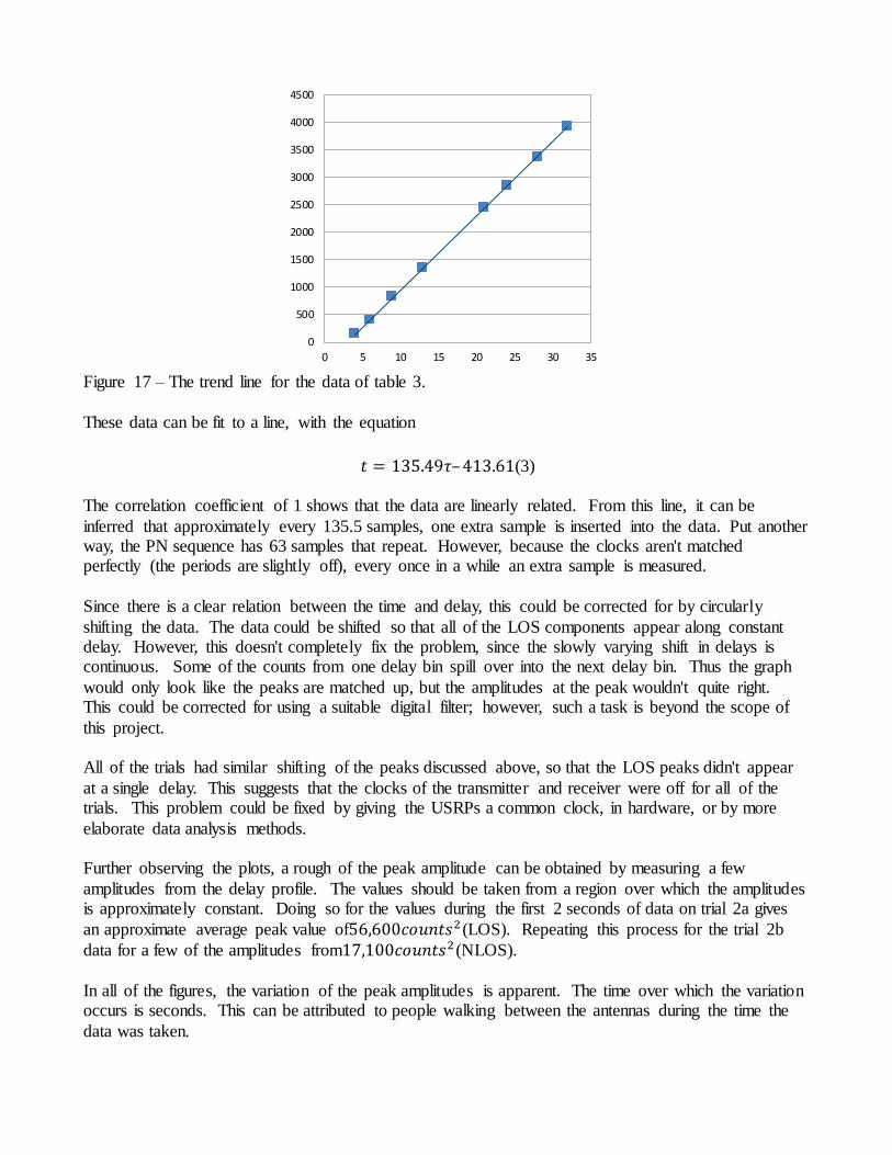
Figure 17 – The trend line for the data of table 3.

These data can be fit to a line, with the equation

𝑡 = 135.49𝜏–413.61(3) The correlation coefficient of 1 shows that the data are linearly related. From this line, it can be

inferred that approximately every 135.5 samples, one extra sample is inserted into the data. Put another way, the PN sequence has 63 samples that repeat. However, because the clocks aren't matched perfectly (the periods are slightly off), every once in a while an extra sample is measured.

Since there is a clear relation between the time and delay, this could be corrected for by circularly

shifting the data. The data could be shifted so that all of the LOS components appear along constant delay. However, this doesn't completely fix the problem, since the slowly varying shift in delays is continuous. Some of the counts from one delay bin spill over into the next delay bin. Thus the graph

would only look like the peaks are matched up, but the amplitudes at the peak wouldn't quite right. This could be corrected for using a suitable digital filter; however, such a task is beyond the scope of

this project. All of the trials had similar shifting of the peaks discussed above, so that the LOS peaks didn't appear

at a single delay. This suggests that the clocks of the transmitter and receiver were off for all of the trials. This problem could be fixed by giving the USRPs a common clock, in hardware, or by more

elaborate data analysis methods. Further observing the plots, a rough of the peak amplitude can be obtained by measuring a few

amplitudes from the delay profile. The values should be taken from a region over which the amplitudes is approximately constant. Doing so for the values during the first 2 seconds of data on trial 2a gives

an approximate average peak value of56,600𝑐𝑜𝑢𝑛𝑡𝑠2 (LOS). Repeating this process for the trial 2b

data for a few of the amplitudes from17,100𝑐𝑜𝑢𝑛𝑡𝑠2 (NLOS).

In all of the figures, the variation of the peak amplitudes is apparent. The time over which the variation occurs is seconds. This can be attributed to people walking between the antennas during the time the

data was taken.

0 5 10 15 20 25 30 35

0

500

1000

1500

2000

2500

3000

3500

4000

4500

A trial with clock synchronization. In the previous section, it was shown that the LOS peaks shifted over time. This was attributed to the

lack of synchronization between the clocks. An additional trial, with PN sequence length 63, clock 32KHz and synchronized clocks, was carried out. The plot of fig. 17a clearly shows that there is not

even a single sample of variation in the location of the LOS peak. Thus the above assertion is correct: a mismatch in the clocks of the receiver and transmitter causes the LOS peaks to shift in time. Note also the constant amplitude of the peak. Recall the assertion that counts spill over between bins,

because of the clock mismatch, causing the peak amplitude to vary. The constant amplitude for the synchronized clock case implies that this assertion is also correct.

Figure 17a – A length 63 PN sequence, with a clock of 32KHz.

With the synchronized clocks, it is also clear that there are multipaths present. It appears that there are

about four multipaths in the above figure. At this point, it is worth mentioning that the trials with mismatched clocks didn't always yield

intelligible data, depending on the USRP boards used. For instance, when the USRP boards with serial numbers 3878 and 3876 were pair as Rx and Tx, respectively, the results were unintelligible. However,

when the USRP boards with serial numbers 3878 and 3874 were used together, as Rx and Tx, respectively, useful data was collected. It may be that board 3876 wasn't functioning properly, or that its clock was too far off from that of the other boards. It appeared to be transmitting, so perhaps the

clock mismatch was too great to get usable data.

The doppler shift.

A trial was done wherein the receiver was moved rapidly back and forth, by hand. In theory, this causes a doppler shift given by

𝑓𝑑 =𝑣

𝜆⋅ cos𝜃(4).

Assuming that the velocity was 2 m/s, and the wavelength (900 MHz carrier) was 0.333 m, and the angle was 0, then the maximum possible doppler shift observable would be f_d = 6 Hz. This is nil compared to the carrier frequency. Thus no appreciable difference would be observed. The CIR of fig.

17b shows a graph very similar to those already seen. Compare this with fig. 13. The only notable difference is that the data appears more "choppy". This might be because the data was taken as

complex, so that the effective sampling rate for the real component was 16KHz instead of 32KHz. Addtionally, if there was a larger doppler shift it still might go unnoticed. The USRP has a phase and

carrier synchronizing component on the RF front end, so that if the frequency changed by small amounts, it would still follow the carrier.

Figure 17b – The Channel impulse response for the case of a moving receiver.

A trial with clock synchronization.

The data of trial 2s was taken with synchronized clocks, with a chip rate (sampling frequency) of 32MHz. As stated in table 1, this gives a resolution which is three orders of magnitude better. With

clock synchronization and this sampling rate, a much better data set will be obtained. This is clear in the plots of fig. 17c-e. The first two plots give the CIR and DP with units of𝑐𝑜𝑢𝑛𝑡𝑠2. The last of these

plots gives the units in level from the peak in dB. This was calculated by dividing the number of counts by the total gain, which was 80 dB, or 10,000, and then plotting it in a log plot. The log plots

reveal much more about the number of multipaths present. The tallest peak is the LOS peak.

Figure 17c – The CIR for trial 2s, with synchronized clocks and 32MHz chip rate.

Figure 17d – The delay profile for trial 2s; units are𝑐𝑜𝑢𝑛𝑡𝑠2.

Figure 17e – The delay profile, in dB, for trial 2s. From the dB plot, it is clear that there are numerous multipaths. This makes sense, since the

experiment was done indoors. One might also wonder why there are so many more multipaths in this case than in [1]. In that paper, the carrier frequency was in the GHz range, while in this paper the

carrier was at the 900 MHz range. The obstacles in a room are different at these frequences. It is worthwhile to inspect this data more. The plots of figs. 17f-h give a plot of the delay profile, and

the autocorrelation in both the time and frequency domain. The delay profile shows the numerous multipaths.

In contrast to what was found in section c, above, it appears that the channel isn't all frequency selective. The channel is somewhere in between flat fading and frequency selective [2], as the shape of

the frequency domain plot of the autocorrelation shows.

Figure 17f – The delay profile for trial 2s.

Figure 17g – The autocorrelation function for trial 2s.

Figure 17h – The autocorrelation for trial 2s, frequency domain.

d. Remaining Station Trials The graphs for the trials at stations 3 and 4 are given in figs. 18 – 25. Once again, the variations in

time, on the order of seconds, in each of the graphs can be attributed to individuals walking about the room during the trial. The data of trial 3a has notably constant peak amplitudes, while the data of trial

4a and 4d have peak amplitudes which vary considerably. The data of trial 4b fits somewhere in between.

What is puzzling about trials 4a and 4b is that 4a had smaller peak amplitudes, and it was supposed to have LOS, while 4b didn't have LOS. It might be that these trials were mixed up, or that the obstacles

in front of the receiver while in position 4a more effectively shielded radiation than the obstacles in front of 4b. Both the 4a and 4d trials have about the same average peak amplitudes, which would be expected, since they were from the same location. It might also be that the Rx gain, which was set by a

lab partner, was set to a value other than 0 dB.

For each of the power delay profiles, the approximate peak amplitudes were found by averaging the peaks over a range of time for which there was roughly no variation. The data is in table 4.

Station Peak Amplitudes in

delay profile (𝐶𝑜𝑢𝑛𝑡𝑠2)

LOS

2a 56600 x

2b 17100

3a 31000 x

3b *

4a 5632 x

4b 16000

4d 4485 x

Table 4 – The approximate peak amplitudes for the delay profiles of the various trials.

Figure 18 – The CIR for the data taken with the receiver at position 3a.

Figure 19 – The DP for the data taken with the receiver at position 3a.

Figure 20 – The CIR for the data taken with the receiver at position 4a.

Figure 21 – The DP for the data taken with the receiver at position 4a.

Figure 22 – The CIR for the data taken with the receiver at position 4b.

Figure 23 – The DP for the data taken with the receiver at position 4b.

Figure 24 – The CIR for the data taken with the receiver at position 4d.

Figure 25 – The DP for the data taken with the receiver at position 4d.

e. Large Scale Fading Unfortunately, the measurements of the 32K sampling rate experiments (placed around the room) weren't sensitive enough to measure the multipath components on the order of nanoseconds. However, some of the data can be analyzed to see what type of fading was present, whether the path loss is inversely proportional to the distance squared, or to the fourth.

For simple LOS path loss, the peak amplitudes should fall off like 1 𝑟2⁄ , while for NLOS path loss, the peak

amplitudes should fall of like1 𝑟4⁄ . Thus for two data points

𝑃1 ∝1

𝑟1𝑛

and

𝑃2 ∝1

𝑟2𝑛.

Taking the ratio of these two, 𝑃1

𝑃2=

𝑟2𝑛

𝑟1𝑛 .

The exponent can be obtained from

𝑛 =log

𝑃1𝑃2

log𝑟2𝑟1

.

The results of the comparison are given in table 4. The powers are obtained from table 4, and the radii are obtained from table 2.

Trials compared

Overall Gain

Ratio of voltages

Ratio of powers, P Ratio of radii, r exponent, n

2a, 3a 80 dB, 80 dB

0.31

0.566

0.3003000 284/511 = 0.555773 2.05

2b, 4b 80dB, 100 dB

0.016

0.171

0.0087671 312/855 = 0.365 4.7

2a, 4a 80 dB, 80 dB

0.05632

0.566

0.0099013 284/845 = 0.3361 4.23

3a, 4a 80 dB, 80 dB

0.05632

0.31

0.0330067 511/845 = 0.605 6.78

Table 5 – Determination of n. For the most part, the above results agree well with the standard models for large scale fading. The comparison of trials 2a and 3a reveals that for LOS the fading is inverse square, as expected for an electromagnetic wave radiating in free space with no obstructions. The comparison of 2b and 4b yields an exponent of 4.7, which isn't

quite a1 𝑟4⁄ dependence. However, it is fairly close, and it also demonstrates that the path loss is much greater in the NLOS case. The last two cases, those comparisons containing trial 4a, don't match up well with the standard models. It may be the case that the data taken for trial 4a, was not LOS. Observing fig. 21, the peaks varied considerably, which indicates NLOS conditions. For this trial, the higher peaks may have been the ones on which to base the estimate of table 4; however, the lower peaks were used because of their roughly constant amplitude.

IV. Conclusion

The sliding correlator channel sounding system was implemented using USRPs for transceiving, and GRC as the frontend for programming the USRPs. Multiple sets of data were taken at different lab

stations in the communications lab. An estimate of the RMS delay spread and coherence bandwidth

were obtained, along with the CIR and Power delay profile. The mismatch of the clocks caused the delays to shift in time, as was verified by doing trials with synchronized clocks. Qualitatively, the power delay profile was as expected: the stations further away from the transmitter had smaller LOS

peaks, and the LOS peaks were larger than the NLOS peaks. The inverse square law was verified, and stronger attenuation was observed for NLOS cases.

By far the biggest hardship for this project was the initial setup. Many different approaches were used, such as reading the data and correlating it in matlab, using different length PN sequences, etc. Only

until much later in the assignment was an effective setup found. Since the point of the project was to focus on the channel effects and not the initial setup, future students might be helped by being provided

with an initial working setup to start from. The texts required for the reading assignment could have been mentioned in the syllabus, so that they could be obtained ahead of time. The USRPs with synchronized clocks could have been provided in a more timely fasion, so that data could be taken from

them earlier on.

An alternative implementation of this system can be obtained from the command line. The gr-sounder folder of the GnuRadio Companion provided an option which avoided the USB bottleneck. With the system used in this paper, the 32MHz sampling rate could be used, but with great latency; the trials

took long to get a decent amount of data. The command line option given in the gr-sound folder can do all of the processing on the USRP board, so that a higher sampling rate can be obtained, and without all

the wait. Data was taken using this approach, but due to time constraints it was not analyzed. Acknowledgments

My thanks to my lab partner, Andre, and Bhargav, who helped with the setup, data taking, and

understanding of the experiment. Thanks also to Professor Sirkeci and the TA for graciously opening the lab for students.

References

[1] M. Gahadza, M. Kim, J. Takada, “Implementation of a Channel Sounder us- ing GNU Radio Opensource SDR Platform,” IEICE Technical Report. available at: http://www.ap.ide.titech.ac.jp/publications/Archive/IEICE_TRSR%280903Mutsa%29.pdf

[2] Wireless Communications, Andrea Goldsmith, Cambridge Press, 2005.

[3] Wireless Communications - Principles and Practice, Theodore Rappaport, 1ed, Prentice Hall, New Jersey, 1999

Appendix – Matlab code