Embed Size (px)
Citation preview
Fuzzy Sets and Systems 161 (2010) 893–918www.elsevier.com/locate/fss
LMI based design of constrained fuzzy predictive controlM. Khairy, A.L. Elshafei, Hassan M. Emara∗
Electrical Power and Machines Department, Faculty of Engineering, Cairo University, Giza 12613, Egypt
Received 20 August 2008; received in revised form 15 September 2009; accepted 26 October 2009Available online 1 November 2009
Abstract
Predictive control of nonlinear systems subject to output and input constraints is considered. A fuzzy model is used to predictthe future behavior. Two new ideas are proposed here. First, an added constraint on the applied control action is used to ensure thedecrease of a quadratic Lyapunov function, and so guarantee Lyapunov exponential stability of the closed-loop system. Second, thefeasibility of the finite-horizon optimization problem with the added constraints is ensured based on an off-line solution of a set ofLMIs. The novel stability method is compared to the existing methods, such as the techniques based on the end-point constraints(terminal constraint set), and the robust stability techniques based on the small gain theory. The proposed method ensures Lyapunovexponential stability, does not need an auxiliary controller and can be used with any feasible controller parameters. Illustrativeexamples including the predictive control of a highly nonlinear chemical reactor (CSTR) are discussed.© 2009 Elsevier B.V. All rights reserved.
Keywords: Model-based predictive control; Receding-horizon control; T–S fuzzy model; LMI
1. Introduction
Model-based predictive control (MBPC) is a popular control algorithm that is based on the use of a model forpredicting the future behavior of the system over a prediction horizon. At each sampling instant, an optimizationproblem is solved on-line over the prediction horizon to obtain the control signal. So, it differs from the conventionalcontrol methods which use a pre-calculated control law. The main reason of the success of this method is the abilityof MBPC to optimally control multivariable systems under constraints. The optimization problem solution depends onthe model nature and the constraints [1]. If the model is linear and there are no constraints, an analytical solution canbe obtained [6,7]. The use of constraints in the predictive control strategy is important. Input constraints give morerealism to the control actions by modeling the saturation and the slew rate constraints in the actuator. Output constraintsare used to ensure a safety operation of the plant [8]. In the presence of constraints, the problem can be formed as aquadratic optimization program for which efficient solution algorithms exist [20]. However, if the model is nonlinear,the optimization problem becomes nonconvex and the solution procedures are complex and time consuming [22]. In[8], three approaches are given to solve this problem in real time generating a suboptimal solution with a performancequite close to the optimal solution.
Fuzzy logic is widely used in MBPC. Its use can be classified into two general classes of approaches [1]. In thefirst class, a fuzzy model is used as a predictor. One advantage of the use of fuzzy models is the fact that they can be
∗ Corresponding author. Tel./fax: + 20 235715920.E-mail address: [email protected] (Hassan M. Emara).
0165-0114/$ - see front matter © 2009 Elsevier B.V. All rights reserved.doi:10.1016/j.fss.2009.10.020
894 M. Khairy et al. / Fuzzy Sets and Systems 161 (2010) 893 –918
constructed using the available information and their complexity can be gradually increased as more information isgathered [8]. The second class of methods depends on the multistage fuzzy decision making [2]. The objective functionand the constraints are fuzzy, while the system model may be fuzzy or nonfuzzy [1,10,18,19,23,31,32,39,42].
The design of stabilizing model-based predictive controllers is the main aim of most researchers in the field duringthe last two decades [22]. In [15], Keerthi and Gilbert used the cost value function as a Lyapunov function for estab-lishing stability of model predictive control of nonlinear discrete time systems (when a terminal equality constraintis used). Techniques based on end point constraints (terminal constraint set) are used to stabilize the MBPC systems[1,5,21,22,24,29]. In these techniques, the purpose of the model predictive controller is to drive the states to a terminalregion where a local stabilizing controller is employed, leading to a dual mode strategy. The main disadvantage of thesetechniques is that there is no guarantee that the fuzzy predictive control drives the states to the terminal region. Oneway to solve the above problem is to choose long prediction horizon, or to gradually increase the prediction horizon,and solve each time the optimization problem, until the states enter the final region [1,29]. Another disadvantage isthat the region of attraction of the auxiliary controller is hardly computable in practice [21]. In [26], constraints onthe control signal and its increment are given to guarantee robust asymptotic stability of the predictive control system.This method can be used only for open loop bounded-input–bounded-output (BIBO) stable processes with an additivel1-norm bounded model uncertainty. Also the added constraints lead to slower response.
In this paper, a novel method is suggested to ensure Lyapunov exponential stability of the closed-loop MBPC system.The idea depends on selecting a quadratic Lyapunov function V (k). An added constraint on the first element of thecontrol sequence vector (applied control action) is used to ensure that V (k + 1) is less than the current value V (k).Among the set of control sequences that achieve the constraints, the control sequence that minimizes the cost functionis selected. Only the first element of the control sequence is applied to the plant and the same procedure is repeated ateach sampling instant (receding-horizon control). A set of LMIs is solved off-line to find the positive definite functionthat ensures the feasibility of the on-line finite horizon optimization problem with the added constraints. This methodis compared to the existing stability methods, such as the terminal constraint set method [1,21], and the robust stabilitytechniques based on the small gain theory [26]. Three illustrative examples are introduced to highlight the advantagesand disadvantages of the different methods.
This paper is organized as follows. The next section introduces the T–S fuzzy model. In Section 3, the problem to besolved is stated. Section 4 discusses the existing stability methods used in MBPC. Section 5 explains the novel methodsuggested to ensure the exponential stability of the MBPC system. In Section 6, three illustrative examples are given.Section 7 concludes this paper.
2. T–S fuzzy models
T–S fuzzy models are suitable for modeling a large class of nonlinear systems [4,9,12,13,35–37,41,43]. They consistof fuzzy IF–THEN rules which represent local linear input–output relations of a nonlinear system. The overall fuzzymodel of the system is achieved by fuzzy blending of the linear system models [36]. In a discrete fuzzy system (DFS),the rules of the T–S fuzzy model take the form [36]
IF z1(t) is Mi1 and . . . and z p(t) is Mip
THENx(t + 1) = Aix(t) + Biu(t)y(t) = Cix(t)
i = 1, 2, . . . , r (1)
where Mi j is the fuzzy set and r is the number of model rules; x(t) ∈ Rn is the state vector, u(t) ∈ Rm is the inputvector, y(t) ∈ Rq is the output vector, Ai ∈ Rn×n , Bi ∈ Rn×m and Ci ∈ Rq×n are the state space matrices of the localsystems; z1(t), . . . , z p(t) are known premise variables that may be functions of the state variables, external disturbancesand time. Given a pair of (x(t), u(t)), the final outputs of the fuzzy system is [36]
x(t + 1) =∑r
i=1 wi (z(t)){Aix(t) + Biu(t)}∑ri=1 wi (z(t))
=r∑
i=1
hi (z(t)){Aix(t) + Biu(t)} (2)
y(t) =∑r
i=1 wi (z(t)){Ci x(t)}∑ri=1 wi (z(t))
=r∑
i=1
hi (z(t)){Ci x(t)} (3)
M. Khairy et al. / Fuzzy Sets and Systems 161 (2010) 893 –918 895
where
wi (z(t)) =p∏
j=1
Mi j (z j (t))
hi (z(t)) = wi (z(t))∑ri=1 wi (z(t))
(4)
The term Mi j (z j (t)) is the grade of membership of z j (t) in Mi j .The following two approaches can be used to obtain the T–S fuzzy model:
1. Identification using input–output data [33,34].2. Derivation from the nonlinear system equations [14,38].
In this paper, the second approach is used to construct the fuzzy model.Sector nonlinearity is a method used to obtain the T–S fuzzy model from the nonlinear system equations. Its idea
first appeared in [14]. Consider a nonlinear system x(t) = f(x(t)), where f(0) = 0. This method finds the global sectorsuch that f(x(t)) ∈ [a1 a2]x(t). Although it guarantees an exact fuzzy model construction, it is sometimes difficult tofind global sectors for general nonlinear systems [36]. This method is used in this paper to obtain the T–S fuzzy modelof the nonlinear system in Example 1.
In [38], the authors showed that the result of Taylor’s linearization of a nonlinear model around an operatingnonequilibrium point is an affine rather than linear model. They suggested a method for constructing local linearmodels that approximate the behavior of the nonlinear system around the operating points. This method is used in thispaper to obtain the T–S fuzzy model of the tank reactor (CSTR) in Example 2.
The modeling performance can be determined by the variance accounted for (VAF) index [27] given by
VAF =[
1 − var(Y − Y)
var(Y)
]× 100% (5)
where Y is the real plant output measurements, Y is the fuzzy model output predictions and var stands for the variance.
3. Problem statement
Consider the nonlinear discrete system:
x(t + 1) = f(x(t), u(t)) (6)
where t is the discrete time index, x(t) ∈ Rn and u(t) ∈ Rm . f is a continuous mapping,
f : Rn × Rm → Rn
It is required to find an optimal control sequence for this system with respect to the following cost function:
J (u(k), x(k), xr(k)) =k+Np∑t=k+1
(xr(t) − x(t))T Q(xr(t) − x(t)) +k+Nc∑t=k
(u(t)T Ru(t) + du(t)T Sdu(t)) (7)
where k is the current sampling instant, J is the cost function, xr is the reference state vector, Np is the predictionhorizon, Nc is the control horizon, du(t) = u(t) − u(t − 1), Q and S are positive semi-definite matrices and R is apositive definite matrix.
The following constraints are taken into account:
ymin ≤ y(t) ≤ ymax ∀t = k + 1, . . . , k + NP
umin ≤ u(t) ≤ umax ∀t = k, . . . , k + Nc(8)
where y is the system output.In this paper, the predictive control strategy is based on a receding-horizon optimization, calculated online at each
sampling instant. The solution of the optimization problem (7) is complicated, because it is a constrained nonlinear
896 M. Khairy et al. / Fuzzy Sets and Systems 161 (2010) 893 –918
optimization problem (nonconvex optimization). The exact solution to this problem cannot be calculated in real time.In [8], three approaches are used to solve this problem in real time generating a suboptimal solution with a performancequite close to the optimal solution. The idea of these approaches is the design of a predictor based on the locallinearization of the system around the current trajectory point. After the predictor is constructed, the optimizationproblem can be formulated as a quadratic program (QP) (see the Appendix). At each sampling instant, the QP problemis solved with new parameters. The three algorithms are based on this concept, but they differ in the way the parametersof the QP are obtained from the nonlinear model.
The approach using a T–S fuzzy model is used in this paper. This approach has the following advantages:
1. No simulation is needed to obtain the QP parameters. The local linear system, used to construct the predictor, canbe generated directly from the inference of the fuzzy system.
2. It is suitable for industry, due to the capacity of the model structure to combine local models identified in experimentsaround the different operating points.
In [8], the stability has not been studied. There is no guarantee that the closed-loop system is asymptotically stable,which is the main disadvantage. In this paper, modifications of the algorithms in [8] are carried out to ensure Lyapunovexponential stability of the closed-loop system. The suggested method will be compared to the existing stabilitymethods, commonly used in MBPC.
In the next section, existing stability methods, used in the framework of MBPC, are discussed briefly.
4. Overview of existing MBPC stability methods
The main objective of the MBPC researchers in the last two decades has been to design a stable MBPC. Mosttechniques depend on adding penalties to the cost function and/or constraints on the states at the end of the predictionhorizon [22]. Also, it is worth mention that there are some fuzzy MBPC methods which depend on using explicitcontrol law (no on-line optimization is needed). Asymptotic stability is achieved in this case under some assumptions[3]. However, this method selects a control law which minimizes the error between the plant output and the output of areference model through a selected coincidence horizon. The proposed fuzzy MBPC adds more flexibility by selectingcontrol actions that minimizes a general cost function in the predicted errors through a prediction horizon, the appliedcontrol actions through a control horizon, and the increments of control actions through a control horizon. Furthermore,the algorithm in [3] guarantees asymptotic stability only for some selections of the coincidence horizon (equal to therelative degree of the system in case of controlling minimum phase plants, and very long coincidence horizons in caseof controlling stable open loop plants). In the following part of this section, two methods will be discussed.
Method M1: In the method, end point constraints are added. The purpose of the predictive controller is to drive thestates to a terminal region, where a local stabilizing controller (u = Kx) is employed (dual mode strategy) [1,21].
The stabilizing nonlinear receding horizon (SNRH) algorithm in [21] is used.The Terminal Constraint Set method has some drawbacks:
1. There is no guarantee that the model predictive controller drives the states to the terminal region [1]. To solve thisproblem, choose long prediction and control horizons. Alternatively, gradually increase the prediction horizon andsolve each time the optimization problem, until the state enters the final region [1,29]. These solutions lead to longcomputational time. The optimization problem may be infeasible to be solved online. In [1], the search using branchand bound method [25] is used to reduce the computational time.
2. The practical computation of the region of attraction of the auxiliary controller is difficult [21].3. The local dynamics of the system differ at the different operating points. The offline calculations should be computed
many times at different reference values.
Method M2: In this method, added constraints on the control signal and its increment are used to achieve robuststability of the MBPC system. To obtain reference error-free tracking, a feed-forward controller is recomputed at eachsampling instant to get unity DC gain between the output and the reference (robust asymptotic stability) [26]. For moreinformation about this method, the reader is referred to [26].
Method M2 has some drawbacks:
1. This method can be used only for open loop bounded-input–bounded-output (BIBO) stable processes.
M. Khairy et al. / Fuzzy Sets and Systems 161 (2010) 893 –918 897
2. Asymptotic stability only is proved (not exponential stability).3. The added constraints on the input and its increment lead to slower response.4. Feed-forward controller with variable gain is needed, which leads to extra online calculations.
In the next section, a novel method is suggested to guarantee Lyapunov exponential stability of the closed-loop system.
5. The proposed design
Consider the nonlinear system (6). It is required to design a stabilizing model based predictive controller for thissystem. The idea depends on adding a constraint to the optimization problem that ensures Lyapunov exponential stabilityof the closed-loop system. Let xe denote the error state vector, so
xe(k) = xr(k) − x(k) (9)
V (k) is a quadratic Lyapunov function, defined as follows:
V (k) = xTe (k)Pxe(k) (10)
where P is a positive definite matrix.
�V (k) = V (k + 1) − V (k) = xTe (k + 1)Pxe(k + 1) − xT
e (k)Pxe(k) (11)
where
xe(k + 1) = xr(k + 1) − x(k + 1)
Starting from any initial states, if it can be proved that �V (k) (shown in (11)) is always negative, V (k) (shown in (10))decreases and xe reaches the origin (asymptotic stability). As V (k) is quadratic, exponential stability is also achieved.
In this paper, the notation Un represents the control sequence. It can be represented as follows:
Un =
⎡⎢⎢⎢⎣
u(k|k)u(k + 1|k)
...
u(k + Nc|k)
⎤⎥⎥⎥⎦
The notation u(k + i |k) means the control action at instant k + i calculated from solving the optimization problem atinstant k.
In MBPC, only the first element of the control sequence vector (u(k|k)) is applied. A constraint is added on u(k|k)to ensure that �V (k) is negative. Among the control sequences that achieve the constraints, the control sequence thatminimizes the cost function (7) is selected. Only the first element of the control sequence is applied to the plant andthe procedure is repeated at each sampling instant.
Definition 1. At instant k, U∗ denotes the set of control sequences that achieve: �V (k) < 0 ∀Un ∈ U∗
Remarks. 1. The nonlinear system (6) under the model based fuzzy predictive control with the following addedconstraint: Un ∈ U∗ is exponentially stable. This can be explained as follows.
Consider the optimization problem at instant k.If the constraint Un ∈ U∗ is achieved, the optimal control sequence will achieve: �V (k) < 0 (from Definition 1).
� V (k + 1) < V (k) (12)
As receding horizon control strategy is used, the same procedure is repeated at each sampling instant, so:
V (k + i) < V (k + i − 1) (13)
where i is a positive integer number.
898 M. Khairy et al. / Fuzzy Sets and Systems 161 (2010) 893 –918
As time goes on, the Lyapunov function V decreases. So, xe will reach the origin (asymptotic stability). As V is aquadratic Lyapunov function (10), exponential decay rate is achieved (exponential stability).
2. If it is required to obtain a certain decay rate to the origin [36], the condition �V (k) < 0 should be modified to:
�V (k) < (�2 − 1)V (k), � < 1 (14)
Different methods are given below for selecting the positive definite matrix P in (10).
Method M3: Select P as a diagonal matrix. The diagonal elements p11, . . . , pnn are positive numbers and are selectedto control the decay rate of different states. For example, if it is required to increase the decay rate of the first state xe1,increase p11. Although this method is simple, there is no guarantee that a feasible control sequence, which achieves�V (k) < 0 and the input constraint (umin ≤ u(k) ≤ umax), is found. Method M4 is introduced to solve this problem.
Method M4: This method is used to guarantee that a feasible solution to the optimization problem with the addedstability constraint is found. The idea of this method is to solve a set of LMIs offline (see Lemma 1 below) to obtain aparallel distributed compensator (PDC) that achieves:
• Exponential stability of the T–S fuzzy model.• The control action is within the saturation limits.
The positive definite matrix P, obtained from the solution of the LMIs, is used in (10). This ensures that at any instantk, at least one feasible control action u(k) exists (equal to the control action obtained from the PDC). This ensures theexponential stability of the closed-loop system.
Lemma 1 (Tanaka and Wang [36]). To obtain a stabilizing parallel distributed compensator (PDC) for the discreteT–S fuzzy system (DFS) in (1), the following LMIs are solved:
Find X > 0 and Mi (i = 1, . . . , r ) satisfying[X XAT
i − MTi BT
iAi X − Bi Mi X
]> 0⎡
⎢⎢⎣ X{
Ai X + A j X − Bi M j − B j Mi
2
}T
{Ai X + A j X − Bi M j − B j Mi
2
}X
⎤⎥⎥⎦ ≥ 0
i < j s.t. hi ∩ h j�∅ (15)
where
X = P−1
Mi = Fi X
Assume that the initial condition x(0) is known, the constraint ‖u(k)‖2 ≤ � is achieved at all times if the followingLMIs are added [36]:[
1 x(0)T
x(0) X
]≥ 0[
X MTi
Mi �2I
]≥ 0 (16)
where Fi is the feedback gain for the fuzzy rule i (i = 1, . . . , r )The feedback gains and a common P can be obtained as
P = X−1
Fi = Mi X−1 (17)
Theorem 1 discusses the feasibility of the optimization problem with the added stability constraint.
M. Khairy et al. / Fuzzy Sets and Systems 161 (2010) 893 –918 899
Theorem 1. Assume that: the LMIs ((15) and (16)) are feasible and the positive definite matrix P in (10) is calculatedusing (17), then: the MBPC optimization problem with the added stability constraint Un ∈ U∗ is always feasible (∀k).
Proof. As the LMIs (15) and (16) are feasible: at any sampling instant k, the control action calculated using the PDCcontrol law (u P DC (k)) satisfies:
• umin ≤ u P DC (k) ≤ umax.• �V (k) < 0.
Consider the optimization problem at instant k:The problem is feasible, if ∃Un that achieves:
• The applied control action (u(k|k)) is: umin ≤ u(k|k) ≤ umax.• �V (k) < 0.
Let U′ denote the set of control sequences that have: u(k|k) = u P DC (k).∀Un ∈ U′, the two feasibility conditions above are achieved.So ∃Un such that the feasibility conditions are achievedSo the optimization problem with the added stability constraint is feasible. �
Method M4 algorithm can be summarized as follows.
Algorithm 1. Offline: Solve the LMIs (15) and (16). Calculate the positive definite matrix P using (17).Online: At each sampling instant, solve the optimization quadratic program with the added stability constraint
(Un ∈ U∗). Only the first element of the optimal control sequence is applied to the plant.
Remarks. 1. To obtain a certain decay rate to the origin, the following GEVP (generalized eigenvalue minimizationproblem) [36] should be solved instead of the LMIs (15).
Let: � = �2, 0 ≤ � < 1
minX,M1,. . .,Mr
�
s.t. X > 0[�X XAT
i − MTi BT
iAi X − Bi Mi X
]> 0⎡
⎢⎢⎣ �X{
Ai X + A j X − Bi M j − B j Mi
2
}T
{Ai X + A j X − Bi M j − B j Mi
2
}X
⎤⎥⎥⎦ ≥ 0
i < j s.t. hi ∩ h j�∅ (18)
where
X = P−1
Mi = Fi X
The sets of LMIs, to be solved, are (16) and (18).In this case, the condition in (14) is used instead of the condition �V (k) < 0.2. The LMIs (15) are conservative. This may result in an infeasible solution. There are many reasons for this
conservatism. First, the used Lyapunov function is quadratic that leads to limited choices. Also, it is difficult to find acommon P which satisfies all conditions, especially in case of using large number of fuzzy rules. Furthermore, LMIconditions are independent of the shape of membership functions that results in more conservatism. Relaxation of LMIconditions has attracted many LMI researchers in the last decade. Several ideas are proposed to relax the LMI conditionsderived in [36]. In [16], an approach is suggested to relax conservatism by representing the interactions among the fuzzysubmodels in a single matrix. In [40], a relaxation technique based on Finsler’s Lemma is proposed that results in simplerand more computationally tractable conditions. In [28], a relaxation method is proposed based on Polya’s theorem. The
900 M. Khairy et al. / Fuzzy Sets and Systems 161 (2010) 893 –918
relaxation is achieved via increasing the number of positivity conditions, and adding artificial decision variables. Incase of using relaxed LMIs that are based on quadratic Lyapunov function (10), it is easy to implement Algorithm A1.This can be achieved by solving the relaxed LMI conditions offline to get P instead of solving the conservative LMIs in[36]. The obtained P is used to construct the Lyapunov function used to form the added stability constraint. Althoughusing relaxed LMIs that depend on quadratic Lyapunov functions and PDC laws results in less conservative conditionscomparing to conditions (15) [36], these relaxed conditions are still conservative because of the limited choices of theLyapunov functions. Consequently, relaxation approaches that are based on using nonquadratic Lyapunov functions areproposed [11,17]. In [11], two different approaches based on nonquadratic Lyapunov functions and non-PDC controllaws are presented. The second approach is the proposed one in [11]. It depends on using nonquadratic Lyapunovfunction, non-PDC control law, and new transformation matrix. In this approach, the candidate Lyapunov function isin the following form [11]:
V (x(k)) = xT (k)
(r∑
i=1
hi (z(k))Gi
)(r∑
i=1
hi (z(k))Pi
)(r∑
i=1
hi (z(k))Gi
)−1
x(k) (19)
where Pi > 0 and Gi = GTi
The general non-PDC control law is given by [11]
u(k) = −(
r∑i=1
hi (z(k))Fi
)(r∑
i=1
hi (z(k))Gi
)−1
x(k) (20)
Lemma 2 (Guerra and Vermeiren [11]). Let (1) be a discrete fuzzy model and consider the control law (20). If thereexists symmetric matrices Pi > 0, matrices Qk
i > 0, Qki j = (Qk
i j )T , j > i , Fi and Gi such that
�kii > Qk
i , i, k = 1, . . . , r
�ki j + �k
ji > Qki j , i, k = 1, . . . , r , j = i + 1, . . . , r
�k =
⎡⎢⎢⎢⎢⎣
2Qk1 (Qk
12)T · · · (Qk1r )T
Qk12 2Qk
2
......
. . . (Qk(r−1)r )T
Qk1r · · · Qk
(r−1)r 2Qkr
⎤⎥⎥⎥⎥⎦ > 0, k = 1, . . . , r (21)
where
�ki j =
[Pi (Ai G j − Bi F j )T
Ai G j − Bi F j Gk + GTk − Pk
], i, j, k = 1, . . . , r
then the closed-loop fuzzy model is globally asymptotically stable.
If it is required to depend on this approach [11] in Algorithm A1, the LMIs (21) are solved offline to obtain Pi ,and Gi where (i = 1, . . . , r ). The feasibility of the LMIs (21) guarantees the existence of a control action at eachsampling instant which decreases the Lyapunov function (19). In the online implementation, the Lyapunov function(19) can be constructed at instant k. This Lyapunov function at the next instant k + 1 can be represented in terms ofthe applied control action u(k|k). An added constraint on the applied control action (the first element in the obtainedcontrol sequence) is used to ensure that �V (k) < 0. This leads to asymptotic stability of the closed loop system.
Method M5: This method is suggested to obtain a decay rate as fast as possible. If the positive definite matrix P,obtained from solving (16) and (18), is used in (10) and the constraint (14) is added to the optimization problem,exponential decay rate (�) is obtained. This decay rate is the fastest, in case of using a unique quadratic Lyapunovfunction. However, there may exist, in some regions, Lyapunov functions that achieve a decay rate faster than � withfeasible control actions. In this method, multiple quadratic Lyapunov functions are used. All these functions are in

M. Khairy et al. / Fuzzy Sets and Systems 161 (2010) 893 –918 901
the form (10), but they have different positive definite matrices (P). This set contains an element PLMI obtained fromthe solution of the LMIs (16) and (18). Assume that the Lyapunov function is changed for each Nd samples. At eachdecision, the Lyapunov function that achieves fastest decay rate during the next Nd samples should be selected.
The method algorithm is shown below. As receding-horizon control strategy is used, the decision is changed eachsampling instant (Nd = 1).
Algorithm 2. Offline: Solve the LMIs (16) and (18) to obtain the positive definite matrix PLMI and the decay rate �.Check that �′ = �
√�max/�min < 1, where �max (�min) is the largest (smallest) eigenvalue of the matrix PLMI.
Define a set of positive definite matrices P = [P1, P2, . . . , PM]. One simple way to construct the set P is to selectdiagonal positive definite matrices. The diagonal elements are selected to indicate various decay rates of the differentstates (as explained before in Method M3).
Online: At each sampling instant k:
1. Assume u(k) = u(k|k − 1) (The second element in Un obtained from the optimization at instant (k − 1).). Using(11), construct a set �V = [�V1(k), �V2(k), . . . , �VM (k)], and a set J1 = [J11, J12, . . . , J1M ] where
J1i = |�Vi (k)|Vi (k)
, Vi (k)�0 (22)
From P, select N positive definite matrices (N < M) that achieve �Vi (k) < 0 and are corresponding to the highestN elements in J1. This approximation is used to obtain from P a smaller set of positive definite matrices. Constructthe following set: P = [P1, . . . , PN, PLMI].
2. The quadratic optimization program with the added constraint (14) is solved (N + 1) times (∀Pi ∈ P). A set of(N + 1) control sequences Un = [Un1, . . . , UnN , UnLMI] is obtained.
3. Construct the set xe = [(‖xe(k+1)‖)1, . . . , (‖xe(k+1)‖)N , (‖xe(k+1)‖)L M I ]. The notation (‖xe(k+1)‖)i representsthe norm of the error state vector at instant k + 1, if the first element of the control sequence vector Uni is appliedto the system at instant k. From Un , select the control sequence Uni that is corresponding to the minimum elementin xe.
4. Apply the first element of the control sequence, obtained from step (3), to the plant.
Remarks.
1. In step 1, from the offline defined set of matrices (P), a smaller set (P) is selected using direct substitution (withoutsolving optimization problems). This is because only finite number of quadratic optimization programs can besolved online (step 2).
2. In step 1, as u(k) has not been determined, the approximation u(k) = u(k|k − 1) is used to obtain �Vi (k). Thisapproximation is also recommended in [8].
3. The positive definite matrix PLMI must be added to the set of positive definite matrices P to ensure the feasibilityof the optimization problem.
4. If N is increased, the computational time increases. Select N that makes the online optimization problem feasible.This selection depends on the sampling interval and the processor used to implement these calculations [8].
5. In step 2, only the feasible control sequences (that achieve the constraints) are considered. Infeasible controlsequences must be rejected from the set. At each sampling instant, at least one feasible control sequence exists(PLMI ∈ P).
Theorem 2 discusses the stability of the closed-loop system, in case of using Algorithm A2 above.
Theorem 2. The nonlinear system (6) under the model based fuzzy predictive control using Algorithm A2 is exponen-tially stable.
Proof. Let ‖xe(k0 + i)‖ denotes the error state vector norm at instant (k0 + i), if Algorithm A2 is used at instant(k0 + i − 1).
902 M. Khairy et al. / Fuzzy Sets and Systems 161 (2010) 893 –918
Starting from any initial states at time k0:If PLMI is used in (10):
(‖xe(k0 + 1)‖)L M I ≤ �′‖xe(k0)‖ (23)
As Pi , selected from the set at time k0, gives minimum ‖xe(k0 + 1)‖:
‖xe(k0 + 1)‖ ≤ (‖xe(k0 + 1)‖)L M I (24)
From (23) and (24):
‖xe(k0 + 1)‖ ≤ �′‖xe(k0)‖ (25)
Consider the optimization problem at instant (k0 + 1), it can be proved in the same way that
‖xe(k0 + 2)‖ ≤ �′‖xe(k0 + 1)‖ (26)
From (25) and (26):
‖xe(k0 + 2)‖ ≤ �′2‖xe(k0)‖ (27)
Consider the optimization problem at instant (k0 + i − 1):It can be proved that
‖xe(k0 + i)‖ ≤ �′i‖xe(k0)‖� �′ < 1, if i → ∞, ‖xe(k0 + i)‖ → 0 (28)
The error state vector will reach the origin exponentially with a decay rate faster than or equal to �′. �
Remark. The condition �′ = �√
�max/�min < 1 must be achieved to complete the proof of Theorem 2. This conditionis calculated offline, so it can be pre-checked to guarantee exponential stability of the closed loop system. In the caseof violation of this condition, a single Lyapunov function based on the solution of LMIs (18) and (16) can be used.During online operation, the optimization problem, with the added stability constraint (14), is solved at each samplinginstant. This ensures exponential stability with decay rate �.
Although the stability analysis that guarantees exponential stability in case of using Algorithm A2 is conservative,Algorithm A2 can achieve exponential stability of the closed loop system even if the above condition on �′ is violated.At each sampling instant k, Algorithm A2 drives the states at k + 1 to a point in the state space nearer to the originthan the point reached by MBPC with the added stability constraint which ensures the decrease of the single Lyapunovfunction obtained from solving LMIs (16) and (18). Consequently, it is logical that if the method based on using thissingle Lyapunov function achieves exponential stability with decay rate �, Algorithm A2 will achieve exponentialstability with a decay rate faster than �.
The novel method, suggested in this paper to ensure the exponential stability of the closed-loop system, has thefollowing advantages:
1. This method achieves exponential stability, while the method suggested in [26] achieves only the asymptotic stability.2. It can be used for any open loop plant type, while the method suggested in [26] can be used only for open loop
BIBO stable processes.3. This method does not need an auxiliary controller. This saves the effort exerted in terminal constraint set methods
[1,21] to determine the practical region of attraction of the local controller.4. This method guarantees the exponential stability of the closed-loop system (assuming that the LMIs (15) and (16)
are feasible). However, in the terminal constraint set methods [1,21], there is no guarantee that MBPC will drivethe states to the terminal region [1].
5. This method can be used for any feasible selection of Np and Nc. In the terminal constraint set methods, Np andNc should be long. If Nc is increased, the number of decision variables in the optimization problem increases. Thisleads to long computational time.
M. Khairy et al. / Fuzzy Sets and Systems 161 (2010) 893 –918 903
Table 1Comparison between the stability method suggested in this paper and the existing stability methods used in MBPC.
Proposed method (M4 andM5)
Method M1 [1,21] Method M2 [26]
Basic theorem Lyapunov stability theorem(Direct method)
Lyapunov stability theorem Small gain theorem
Stability type Exponential stability Depends on the algorithm:In [1], asymptotic stability isproved, while in [21], expo-nential stability
Robust asymptotic stability
Open loop plant Any plant Any plant BIBO stable processes onlyAuxiliary controller No need Local stabilizing controller
nearby the originFeed-forward controller withvariable gain to get offset freetracking
MBPC parameters (Np and Nc) Any feasible values Should be long Any feasible valuesStability guarantee Exponential stability is en-
sured (assume that the LMIproblem is feasible)
No guarantee that the MBPCwill drive the states to the ter-minal region [1]
If the uncertainty is lessthan the upper bound, robustasymptotic stability is ensured
Table 1 summarizes the differences between the proposed method and the existing stability methods (Methods M1and M2).
In the next section, three illustrative examples are given to test the novel stability method and to highlight thedifferences between it and the other existing stability methods.
6. Illustrative examples
In this section, the optimizations required by the different methods were performed using the MATLAB® software.
6.1. Example 1
This example is given to show the advantages of the proposed design, compare it to the terminal constraint setmethod, and study the effect of the proposed added stability constraint on the computational effort.
Consider the nonlinear system shown in (29). It is required to design a stabilizing MBPC for this system.
x1 = x2
x2 = −0.1x1 − x32 + u
y = x1
x1 ∈ [−2, 2]
x2 ∈ [−1, 1] (29)
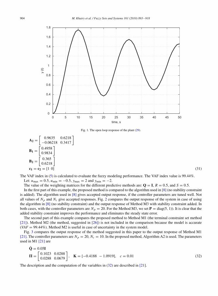
The open loop step response of the plant is shown in Fig. 1.Using sector nonlinearity, the continuous T–S fuzzy model of the above system is obtained. Assume T = 1 s, the
discrete T–S fuzzy model is:If z is M1 then x(k + 1) = A1x(k) + B1u(k)
y(k) = c1x(k)
If z is M2 then x(k + 1) = A2x(k) + B2u(k)
y(k) = c2x(k) (30)
where z = −x22 , M1 = z + 1 and M2 = −z.
A1 =[
0.9504 0.9834−0.09834 0.9504
]
904 M. Khairy et al. / Fuzzy Sets and Systems 161 (2010) 893 –918
0 5 10 15 20 25 30 35 40 45 500
0.2
0.4
0.6
0.8
1
1.2
1.4
1.6
1.8
time, s
y (t)
Fig. 1. The open loop response of the plant (29).
A2 =[
0.9635 0.6218−0.06218 0.3417
]
B1 =[
0.49580.9834
]
B2 =[
0.3650.6218
]c1 = c2 = [1 0] (31)
The VAF index in (5) is calculated to evaluate the fuzzy modeling performance. The VAF index value is 99.44%.Let: umax = 0.5, umin = −0.5, ymax = 2 and ymin = −2.The value of the weighting matrices for the different predictive methods are: Q = I, R = 0.5, and S = 0.5.In the first part of this example, the proposed method is compared to the algorithm used in [8] (no stability constraint
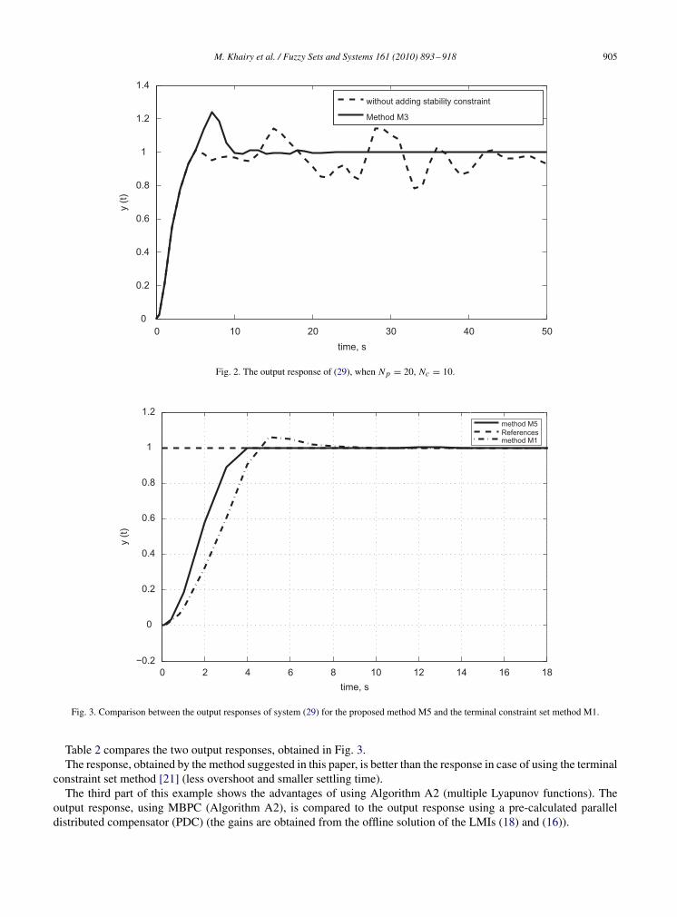
is added). The algorithm used in [8] gives accepted output response, if the controller parameters are tuned well. Notall values of Np and Nc give accepted responses. Fig. 2 compares the output response of the system in case of usingthe algorithm in [8] (no stability constraint) and the output response of Method M3 with stability constraint added. Inboth cases, with the controller parameters are Np = 20. For the Method M3, we set P = diag(5, 1)). It is clear that theadded stability constraint improves the performance and eliminates the steady state error.
The second part of this example compares the proposed method to Method M1 (the terminal constraint set method[21]). Method M2 (the method, suggested in [26]) is not included in the comparison because the model is accurate(VAF = 99.44%). Method M2 is useful in case of uncertainty in the system model.
Fig. 3 compares the output response of the method suggested in this paper to the output response of Method M1[21]. The controller parameters are Np = 20, Nc = 10. In the proposed method, Algorithm A2 is used. The parametersused in M1 [21] are
Q = 0.05I
P =[
0.1023 0.02880.0288 0.0679
], K = [−0.4188 − 1.0919], c = 0.01 (32)
The description and the computation of the variables in (32) are described in [21].
M. Khairy et al. / Fuzzy Sets and Systems 161 (2010) 893 –918 905
0 10 20 30 40 500
0.2
0.4
0.6
0.8
1
1.2
1.4
time, s
y (t)
without adding stability constraint
Method M3
Fig. 2. The output response of (29), when Np = 20, Nc = 10.
0 2 4 6 8 10 12 14 16 18−0.2
0
0.2
0.4
0.6
0.8
1
1.2
time, s
y (t)
method M5Referencesmethod M1
Fig. 3. Comparison between the output responses of system (29) for the proposed method M5 and the terminal constraint set method M1.
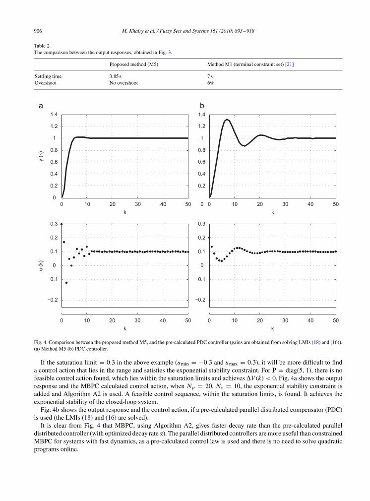
Table 2 compares the two output responses, obtained in Fig. 3.The response, obtained by the method suggested in this paper, is better than the response in case of using the terminal
constraint set method [21] (less overshoot and smaller settling time).The third part of this example shows the advantages of using Algorithm A2 (multiple Lyapunov functions). The
output response, using MBPC (Algorithm A2), is compared to the output response using a pre-calculated paralleldistributed compensator (PDC) (the gains are obtained from the offline solution of the LMIs (18) and (16)).
906 M. Khairy et al. / Fuzzy Sets and Systems 161 (2010) 893 –918
Table 2The comparison between the output responses, obtained in Fig. 3.
Proposed method (M5) Method M1 (terminal constraint set) [21]
Settling time 3.85 s 7 sOvershoot No overshoot 6%
0 10 20 30 40 50
−0.2
−0.1
0
0.1
0.2
0.3
k
u (k
)
0 10 20 30 40 50
−0.2
−0.1
0
0.1
0.2
0.3
k
0 10 20 30 40 500
0.2
0.4
0.6
0.8
1
1.2
1.4
k
y (k
)
0 10 20 30 40 500
0.2
0.4
0.6
0.8
1
1.2
1.4
k
Fig. 4. Comparison between the proposed method M5, and the pre-calculated PDC controller (gains are obtained from solving LMIs (18) and (16)).(a) Method M5 (b) PDC controller.
If the saturation limit = 0.3 in the above example (umin = −0.3 and umax = 0.3), it will be more difficult to finda control action that lies in the range and satisfies the exponential stability constraint. For P = diag(5, 1), there is nofeasible control action found, which lies within the saturation limits and achieves �V (k) < 0. Fig. 4a shows the outputresponse and the MBPC calculated control action, when Np = 20, Nc = 10, the exponential stability constraint isadded and Algorithm A2 is used. A feasible control sequence, within the saturation limits, is found. It achieves theexponential stability of the closed-loop system.
Fig. 4b shows the output response and the control action, if a pre-calculated parallel distributed compensator (PDC)is used (the LMIs (18) and (16) are solved).
It is clear from Fig. 4 that MBPC, using Algorithm A2, gives faster decay rate than the pre-calculated paralleldistributed controller (with optimized decay rate �). The parallel distributed controllers are more useful than constrainedMBPC for systems with fast dynamics, as a pre-calculated control law is used and there is no need to solve quadraticprograms online.
M. Khairy et al. / Fuzzy Sets and Systems 161 (2010) 893 –918 907
Table 3Study of the influence of the added stability constraint on the computational time of QP.
Np 10 10 10 15 15 20 20Nc 5 6 8 5 10 10 15Average time (s) (without stability constraint) 0.025 0.038 0.043 0.040 0.111 0.120 0.171Percentage increase due to the added stability constraint (%) 2 6 11 20 19 14 18
Table 4CSTR parameters.
Parameter Description Nominal value
Ca0 Inlet feed concentration 0.5 mol/lT0 Feed temperature 350 Kq Process flow rate 100 l/minV Reactor volume 100 l� Liquid density 1000 g/lC p Specific heat 0.239 J/g K�H Heat of reaction −50 000 J/molE/R Activation energy 8750 KUA Heat transfer coefficient 50 000 J/min Kk0 Reaction rate constant 7.2 × 10¹⁰ min−1
The last part of this example studies the effect of the added stability constraint on the computational time of solvingthe online quadratic program. Indeed, it is difficult to determine this effect analytically. As a result, an experimentalstudy is carried out to determine the influence of the added stability constraint on computational time. Table 3 shows fordifferent selections of Np, and Nc the average computational time of online QP without the added stability constraint,and the percentage increase in the average computational time of the online QP due to the added stability constraint.In this study, Algorithm A1 was used to find P required for constructing the stability constraint. The computer, used inthe study, was a dual Pentium 4, 3.2 GHz, 1 GB RAM.
It is noticed from the study that the added stability constraint increases the computational time, and this increase isapproximately in the range of [1–20%].
6.2. Example 2
In this example, the control of a highly nonlinear model of a continuous stirred tank reactor (CSTR) [30] is discussed.Assuming constant liquid volume, the CSTR is described by the following dynamic model:
Ca = q
V(Ca0 − Ca) − k0 exp
(− E
RT
)Ca
T = q
V(T0 − T ) + (−�H )
�C pk0 exp
(− E
RT
)Ca + U A
V �CP(Tc − T ) (33)
The above model represents an exothermic, irreversible reaction, A → B, and it is based on a component balance forreactant A and an energy balance. Ca is the concentration of A in the reactor, T is the reactor temperature and Tc is thetemperature of the coolant stream. The description and the numerical values of the different parameters are shown inTable 4.
It is required to design a stabilizing MBPC for the above system. The constraints are
230 ≤ Tc ≤ 370 K, 260 ≤ T ≤ 380 K, 0 ≤ Ca ≤ 1 mol/l
Let: x1 = ca − caeq , x2 = T − Teq and u = Tc − Tceq , where Caeq , Teq and Tceq represent the required equilibriumvalues of concentration, temperature and coolant temperature, respectively.
908 M. Khairy et al. / Fuzzy Sets and Systems 161 (2010) 893 –918
0 5 10 15 20 25 30 35200
220
240
260
280
300
time, min
T C
0 5 10 15 20 25 30 35−10
−5
0
5
10
15
20
25
time, min
erro
r, %
Concentration, caReactor Temprature, T
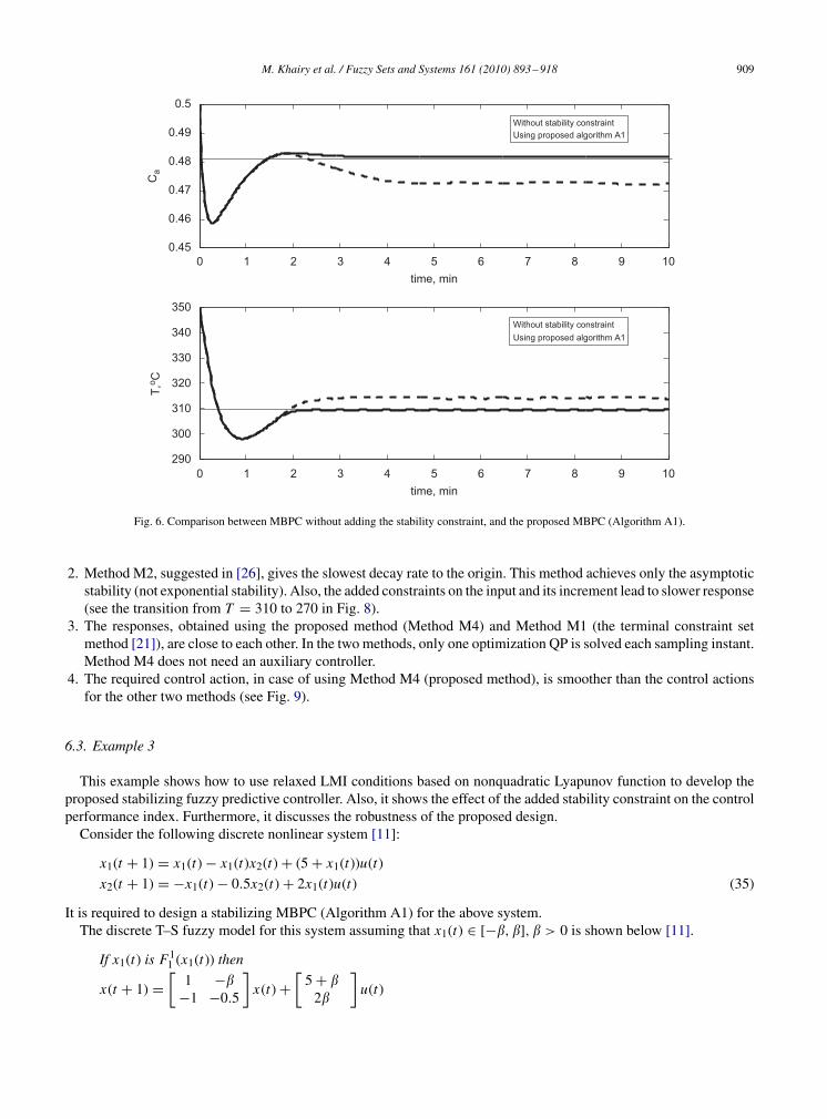
Fig. 5. The validation test of the T–S fuzzy model (CSTR example), the input coolant temperature (upper plot) and the percentage error in theconcentration and temperature (lower plot).
The method, suggested in [38] to obtain local linear models around the nonequilibrium operating points, is usedto determine the continuous T–S fuzzy model that represents the CSTR system. Assume that T = 5 s, the discreteT–S fuzzy model is obtained. Fig. 5 shows the input test signal used in the validation test, the percentage error in theconcentration and the percentage error in the reactor temperature. The VAF index value is 98.22%.
The value of the weighting matrices for the different predictive methods are
Q =[
1 0
01
350
], R = 1
300and S = 0.1
The first part of this example compares Method M4 (the proposed method, Algorithm A1 is applied) to the methodsuggested in [8] (stability constraint is not added). The controllers’ parameters are: Np = 10 and Nc = 9. Fig.6 indicates that for both the concentration and the reactor temperature, the added exponential stability constraintimproves the performance and eliminates the steady state errors.
The second part of this example compares the method suggested in this paper to the existing stability methods,explained in Section 4.
For the proposed method M4, Algorithm A1 is used. For Method M1, suggested in [21]:
Q = 0.05I, c = 0.1 (34)
The description and the computation of the variables in (34) are described in [21].For Method M2 [26], the uncertainty in the model matrices (DA(k) andDB(k)) are obtained as a convex combination
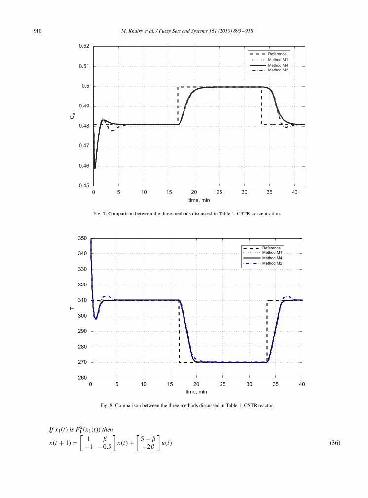
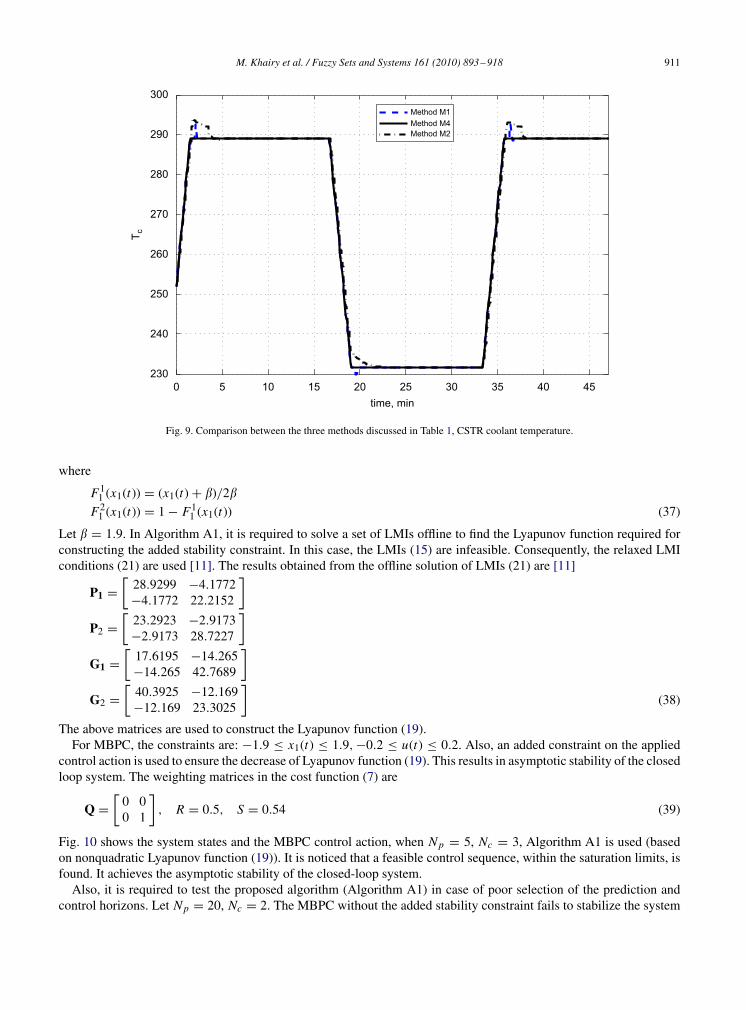
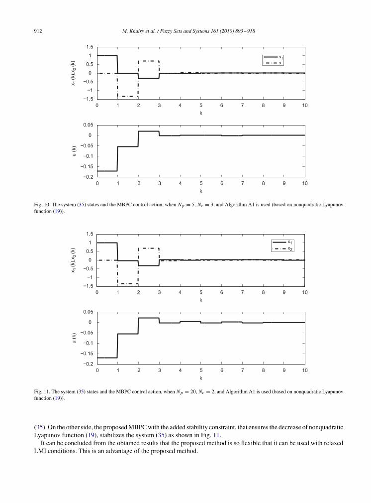
of the local uncertainties of the different fuzzy rules [8, Chapter 7].It can be noted, from Figs. 7 to 9, that:
1. The steady state errors equal to zero in the three methods (asymptotic stability).
M. Khairy et al. / Fuzzy Sets and Systems 161 (2010) 893 –918 909
0 1 2 3 4 5 6 7 8 9 10290
300
310
320
330
340
350
time, min
T,o C
0 1 2 3 4 5 6 7 8 9 100.45
0.46
0.47
0.48
0.49
0.5
time, min
Ca
Without stability constraintUsing proposed algorithm A1
Without stability constraintUsing proposed algorithm A1
Fig. 6. Comparison between MBPC without adding the stability constraint, and the proposed MBPC (Algorithm A1).
2. Method M2, suggested in [26], gives the slowest decay rate to the origin. This method achieves only the asymptoticstability (not exponential stability). Also, the added constraints on the input and its increment lead to slower response(see the transition from T = 310 to 270 in Fig. 8).
3. The responses, obtained using the proposed method (Method M4) and Method M1 (the terminal constraint setmethod [21]), are close to each other. In the two methods, only one optimization QP is solved each sampling instant.Method M4 does not need an auxiliary controller.
4. The required control action, in case of using Method M4 (proposed method), is smoother than the control actionsfor the other two methods (see Fig. 9).
6.3. Example 3
This example shows how to use relaxed LMI conditions based on nonquadratic Lyapunov function to develop theproposed stabilizing fuzzy predictive controller. Also, it shows the effect of the added stability constraint on the controlperformance index. Furthermore, it discusses the robustness of the proposed design.
Consider the following discrete nonlinear system [11]:
x1(t + 1) = x1(t) − x1(t)x2(t) + (5 + x1(t))u(t)
x2(t + 1) = −x1(t) − 0.5x2(t) + 2x1(t)u(t) (35)
It is required to design a stabilizing MBPC (Algorithm A1) for the above system.The discrete T–S fuzzy model for this system assuming that x1(t) ∈ [−�, �], � > 0 is shown below [11].
If x1(t) is F11 (x1(t)) then
x(t + 1) =[
1 −�−1 −0.5
]x(t) +
[5 + �
2�
]u(t)
910 M. Khairy et al. / Fuzzy Sets and Systems 161 (2010) 893 –918
0 5 10 15 20 25 30 35 400.45
0.46
0.47
0.48
0.49
0.5
0.51
0.52
time, min
Ca
ReferenceMethod M1Method M4Method M2
Fig. 7. Comparison between the three methods discussed in Table 1, CSTR concentration.
0 5 10 15 20 25 30 35 40260
270
280
290
300
310
320
330
340
350
time, min
T
ReferenceMethod M1Method M4Method M2
Fig. 8. Comparison between the three methods discussed in Table 1, CSTR reactor.
If x1(t) is F21 (x1(t)) then
x(t + 1) =[
1 �−1 −0.5
]x(t) +
[5 − �−2�
]u(t) (36)
M. Khairy et al. / Fuzzy Sets and Systems 161 (2010) 893 –918 911
0 5 10 15 20 25 30 35 40 45230
240
250
260
270
280
290
300
time, min
T c
Method M1Method M4Method M2
Fig. 9. Comparison between the three methods discussed in Table 1, CSTR coolant temperature.
where
F11 (x1(t)) = (x1(t) + �)/2�
F21 (x1(t)) = 1 − F1
1 (x1(t)) (37)
Let � = 1.9. In Algorithm A1, it is required to solve a set of LMIs offline to find the Lyapunov function required forconstructing the added stability constraint. In this case, the LMIs (15) are infeasible. Consequently, the relaxed LMIconditions (21) are used [11]. The results obtained from the offline solution of LMIs (21) are [11]
P1 =[
28.9299 −4.1772−4.1772 22.2152
]
P2 =[
23.2923 −2.9173−2.9173 28.7227
]
G1 =[
17.6195 −14.265−14.265 42.7689
]
G2 =[
40.3925 −12.169−12.169 23.3025
](38)
The above matrices are used to construct the Lyapunov function (19).For MBPC, the constraints are: −1.9 ≤ x1(t) ≤ 1.9, −0.2 ≤ u(t) ≤ 0.2. Also, an added constraint on the applied
control action is used to ensure the decrease of Lyapunov function (19). This results in asymptotic stability of the closedloop system. The weighting matrices in the cost function (7) are
Q =[
0 00 1
], R = 0.5, S = 0.54 (39)
Fig. 10 shows the system states and the MBPC control action, when Np = 5, Nc = 3, Algorithm A1 is used (basedon nonquadratic Lyapunov function (19)). It is noticed that a feasible control sequence, within the saturation limits, isfound. It achieves the asymptotic stability of the closed-loop system.
Also, it is required to test the proposed algorithm (Algorithm A1) in case of poor selection of the prediction andcontrol horizons. Let Np = 20, Nc = 2. The MBPC without the added stability constraint fails to stabilize the system
912 M. Khairy et al. / Fuzzy Sets and Systems 161 (2010) 893 –918
0 1 2 3 4 5 6 7 8 9 10−1.5
−1
−0.5
0
0.5
1
1.5
k
x 1 (k
),x2
(k)
0 1 2 3 4 5 6 7 8 9 10−0.2
−0.15
−0.1
−0.05
0
0.05
k
u (k
)
x1x
Fig. 10. The system (35) states and the MBPC control action, when Np = 5, Nc = 3, and Algorithm A1 is used (based on nonquadratic Lyapunovfunction (19)).
0 1 2 3 4 5 6 7 8 9 10−1.5
−1
−0.5
0
0.5
1
1.5
k
x 1 (k
),x2
(k)
0 1 2 3 4 5 6 7 8 9 10−0.2
−0.15
−0.1
−0.05
0
0.05
k
u (k
)
x1x2
Fig. 11. The system (35) states and the MBPC control action, when Np = 20, Nc = 2, and Algorithm A1 is used (based on nonquadratic Lyapunovfunction (19)).
(35). On the other side, the proposed MBPC with the added stability constraint, that ensures the decrease of nonquadraticLyapunov function (19), stabilizes the system (35) as shown in Fig. 11.
It can be concluded from the obtained results that the proposed method is so flexible that it can be used with relaxedLMI conditions. This is an advantage of the proposed method.
M. Khairy et al. / Fuzzy Sets and Systems 161 (2010) 893 –918 913
Table 5Comparison of performance indices at different sampling instants for three cases: global solution of (7) obtained offline, suboptimal solution of (7)obtained online (no stability constraint), and suboptimal solution of (7) obtained online (with stability constraint).
Sampling instant SolutionGlobal minimum of (7) calculated of-fline
Approximated solution of (7) obtainedonline (no stability constraint)
Approximated solution of (7) obtainedonline (with stability constraint)
0 1.4 7.1 7.651 0.1 0.826 0.52 0.005 0.0105 0.005153 1.4 × 10⁻⁴ 4.4 × 10⁻⁴ 7.5 × 10⁻⁴
4 4.2 × 10⁻⁶ 5.4 × 10⁻⁵ 1.4 × 10⁻⁵
5 1.43 × 10⁻⁶ 1.83 × 10⁻⁶ 10−5
6 0.75 × 10⁻⁶ 10−6 0.8 × 10⁻⁵
In the second part of this example, the effect of the added stability constraint on the performance index (7) is studied.Table 5 compares performance indices obtained from solving (7) at different sampling instants for three cases at Np = 5,Nc = 3.
1. The global minimum of the optimization problem (7) obtained offline (no stability constraint).2. The suboptimal solution of the optimization problem (7) obtained from solving QP online (no stability constraint).3. The suboptimal solution of the optimization problem (7) obtained online (with stability constraint).
Remarks.1. It is clear that the global solution of the constrained nonlinear optimization problem (7) gives minimum performance
index. However, as stated before the optimization problem is nonconvex and it cannot be implemented online.2. The online solution of QP without stability constraint gives performance index at instant k less than the one obtained
online with stability constraint, if the current system states at instant k are the same for the two cases (such as atinstant 0). This is expected as in the proposed method the control action is selected from a set U∗ which is a subsetof the admissible set for control actions in case of MBPC without stability constraint. However, the increase in theperformance index also happens in the existing stability methods (Methods M1 and M2) as the control sequence isselected from a set that achieves stability constraints. Similarly, this set is a subset of the admissible set for controlsequences when no stability constraint is used (within saturation limits).
3. If the current system states at instant k for these two cases differ, the proposed method may give less performanceindex (7) than the solution of QP without stability constraint (such as at instants 1 and 2).
4. As receding-horizon control strategy is used, only the first element of the optimal control sequence at any instant kis applied to the system. Consequently, the method that has minimum value of (7) at instant k is not necessary thebest one. It may give output error at instant k + 1 higher than other methods. As a result, the best way to calculatethe performance index is to run the system over the prediction horizon, and substitute with the obtained values ofstates and inputs in (7). For Np = 5, Nc = 3: the values of (7) are: (for the approximated method without stabilityconstraint = 2.82, and with stability constraint = 2.32). The proposed method gives better performance.
The last part of this example discusses the robustness of the proposed method. In other words, what is the effectof uncertainty in the system model and external disturbances on the system stability? System (35) is unstable system,so the controlled system is sensitive to uncertainty in the model parameters and external disturbances. To discuss therobustness aspects, let us assume that (36) is derived based on wrong information about the system, and the actualsystem equations are shown below.
x1(t + 1) = x1(t) − x1(t)x2(t) + (7.5 + x1(t))u(t)
x2(t + 1) = −x1(t) − 0.5x2(t) + 2x1(t)u(t) (40)
In this case, using control law (20) results in unstable closed loop system. On the other hand, Fig. 12 shows the statesand the control action in case of using the proposed fuzzy predictive controller (Algorithm A1, Np = 5, Nc = 3).
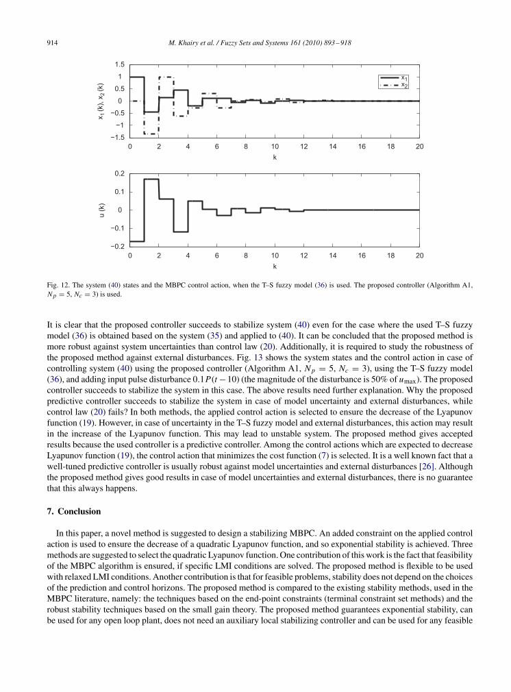
914 M. Khairy et al. / Fuzzy Sets and Systems 161 (2010) 893 –918
0 2 4 6 8 10 12 14 16 18 20−0.2
−0.1
0
0.1
0.2
k
u (k
)
0 2 4 6 8 10 12 14 16 18 20−1.5
−1
−0.5
0
0.5
1
1.5
k
x 1 (k
), x 2
(k)
x1x2
Fig. 12. The system (40) states and the MBPC control action, when the T–S fuzzy model (36) is used. The proposed controller (Algorithm A1,Np = 5, Nc = 3) is used.
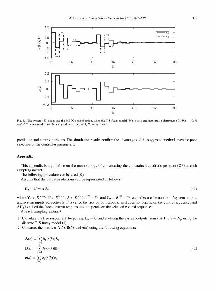
It is clear that the proposed controller succeeds to stabilize system (40) even for the case where the used T–S fuzzymodel (36) is obtained based on the system (35) and applied to (40). It can be concluded that the proposed method ismore robust against system uncertainties than control law (20). Additionally, it is required to study the robustness ofthe proposed method against external disturbances. Fig. 13 shows the system states and the control action in case ofcontrolling system (40) using the proposed controller (Algorithm A1, Np = 5, Nc = 3), using the T–S fuzzy model(36), and adding input pulse disturbance 0.1P(t −10) (the magnitude of the disturbance is 50% of umax). The proposedcontroller succeeds to stabilize the system in this case. The above results need further explanation. Why the proposedpredictive controller succeeds to stabilize the system in case of model uncertainty and external disturbances, whilecontrol law (20) fails? In both methods, the applied control action is selected to ensure the decrease of the Lyapunovfunction (19). However, in case of uncertainty in the T–S fuzzy model and external disturbances, this action may resultin the increase of the Lyapunov function. This may lead to unstable system. The proposed method gives acceptedresults because the used controller is a predictive controller. Among the control actions which are expected to decreaseLyapunov function (19), the control action that minimizes the cost function (7) is selected. It is a well known fact that awell-tuned predictive controller is usually robust against model uncertainties and external disturbances [26]. Althoughthe proposed method gives good results in case of model uncertainties and external disturbances, there is no guaranteethat this always happens.
7. Conclusion
In this paper, a novel method is suggested to design a stabilizing MBPC. An added constraint on the applied controlaction is used to ensure the decrease of a quadratic Lyapunov function, and so exponential stability is achieved. Threemethods are suggested to select the quadratic Lyapunov function. One contribution of this work is the fact that feasibilityof the MBPC algorithm is ensured, if specific LMI conditions are solved. The proposed method is flexible to be usedwith relaxed LMI conditions. Another contribution is that for feasible problems, stability does not depend on the choicesof the prediction and control horizons. The proposed method is compared to the existing stability methods, used in theMBPC literature, namely: the techniques based on the end-point constraints (terminal constraint set methods) and therobust stability techniques based on the small gain theory. The proposed method guarantees exponential stability, canbe used for any open loop plant, does not need an auxiliary local stabilizing controller and can be used for any feasible
M. Khairy et al. / Fuzzy Sets and Systems 161 (2010) 893 –918 915
0 5 10 15 20 25 30−1.5
−1
−0.50
0.5
1
1.5
k
x 1 (k
),x2
(k)
0 5 10 15 20 25 30−0.2
−0.1
0
0.1
0.2
k
u (k
)
x1x2
Fig. 13. The system (40) states and the MBPC control action, when the T–S fuzzy model (36) is used and input pulse disturbance 0.1P(t − 10) isadded. The proposed controller (Algorithm A1, N p = 5, Nc = 3) is used.
prediction and control horizons. The simulation results confirm the advantages of the suggested method, even for poorselection of the controller parameters.
Appendix
This appendix is a guideline on the methodology of constructing the constrained quadratic program (QP) at eachsampling instant.
The following procedure can be used [8]:Assume that the output predictions can be represented as follows:
Yn = C+ KUn (41)
where Yn ∈ RNP no ,C ∈ RNP no ,K ∈ RNP no×(Nc+1)ni , and Un ∈ R(Nc+1)ni . no and ni are the number of system outputsand system inputs, respectively. C is called the free output response as it does not depend on the control sequence, andKUn is called the forced output response as it depends on the selected control sequence.
At each sampling instant k:
1. Calculate the free response C by putting Un = 0, and evolving the system outputs from k + 1 to k + Np using thediscrete T–S fuzzy model (1).
2. Construct the matrices A(k), B(k), and c(k) using the following equations:
A(k) =r∑
i=1hi (z(k))Ai
B(k) =r∑
i=1hi (z(k))Bi
c(k) =r∑
i=1hi (z(k))ci
(42)
916 M. Khairy et al. / Fuzzy Sets and Systems 161 (2010) 893 –918
3. Use A(k), B(k), and c(k) to construct the matrix K:
K = [CnH 0] (43)
where
Cn =
⎡⎢⎢⎢⎣
c(k) 0 . . . 00 c(k) . . . 0...
.... . .
...
0 0 . . . c(k)
⎤⎥⎥⎥⎦ ∈ RNP no×NP nS (44)
H =
⎡⎢⎢⎢⎢⎢⎢⎢⎢⎢⎢⎣
B(k) 0 . . . 0A(k)B(k) B(k) . . . 0
......
. . ....
ANP−2(k)B(k) ANP−3(k)B(k) . . .NP−Nc−1∑
i=0Ai (k)B(k)
ANP−1(k)B(k) ANP−2(k)B(k) . . .NP−Nc∑
i=0Ai (k)B(k)
⎤⎥⎥⎥⎥⎥⎥⎥⎥⎥⎥⎦
∈ RNP nS×Ncni (45)
where ns is the system order.4. The QP is
J (Un) = Jmin + 2[(C− Yre f )T Q1K− UTk−1S1D]Un + UT
n [KT Q1K+ R1 + DT S1D]Un (46)
where
Jmin = YTre f Q1Yre f + CT Q1C− 2YT
re f Q1C+ UTk−1S1Uk−1 (47)
Q1 =
⎡⎢⎢⎢⎣
Q 0 . . . 00 Q . . . 0...
.... . .
...
0 0 . . . Q
⎤⎥⎥⎥⎦ ∈ RNP no×NP no (48)
S1 =
⎡⎢⎢⎢⎣
S 0 . . . 00 S . . . 0...
.... . .
...
0 0 . . . S
⎤⎥⎥⎥⎦ ∈ R(Nc+1)ni ×(Nc+1)ni (49)
R1 =
⎡⎢⎢⎢⎣
R 0 . . . 00 R . . . 0...
.... . .
...
0 0 . . . R
⎤⎥⎥⎥⎦ ∈ R(Nc+1)ni ×(Nc+1)ni (50)
Uk−1 =
⎡⎢⎢⎢⎣
u(k − 1)0...
0
⎤⎥⎥⎥⎦ ∈ R(Nc+1)ni (51)
D =
⎡⎢⎢⎢⎢⎢⎣
I 0 0 · · · 0−I I 0 · · · 00 −I I · · · 0...
.... . .
. . ....
0 0 0 −I I
⎤⎥⎥⎥⎥⎥⎦ ∈ R(Nc+1)ni ×(Nc+1)ni (52)
M. Khairy et al. / Fuzzy Sets and Systems 161 (2010) 893 –918 917
Yre f is the vector of reference values of the outputs during the prediction horizon
Yre f =
⎡⎢⎣
yre f (k + 1)...
yre f (k + Np)
⎤⎥⎦ ∈ RNP no (53)
The input and output constraints can be represented as follows:⎡⎢⎢⎣
I−IK
−K
⎤⎥⎥⎦Un ≤
⎡⎢⎢⎣
Umax−Umin
Ymax − �−Ymin + �
⎤⎥⎥⎦ (54)
where
Ymin =
⎡⎢⎣
ymin(k + 1)...
ymin(k + Np)
⎤⎥⎦ ∈ RNP no
Ymax =
⎡⎢⎣
ymax(k + 1)...
ymax(k + Np)
⎤⎥⎦ ∈ RNP no
Umin =
⎡⎢⎣
umin(k)...
umin(k + Nc)
⎤⎥⎦ ∈ R(Nc+1)ni
Umax =
⎡⎢⎣
umax(k)...
umax(k + Nc)
⎤⎥⎦ ∈ R(Nc+1)ni (55)
The QP ((46) with the added constraints (54)) is solved to get the optimal control sequence. The same procedure isrepeated at each sampling instant.
An added stability constraint should be added to the input and output constraints, if it is required to guaranteeasymptotic stability of the closed loop system.
References
[1] K. Belarbi, F. Megri, A stable model-based fuzzy predictive control based on fuzzy dynamic programming, IEEE Trans. Fuzzy systems 15 (4)(2007) 746–754.
[2] R.E. Bellman, L. Zadeh, Decision-making in a fuzzy environment, Manage. Sci. 17 (1970) 141–164.[3] S. Blazic, I. Skrjanc, Design and stability analysis of fuzzy model-based predictive control—a case study, J. Intelligent Robotic Syst. 49 (3)
(2007) 279–292.[4] S.G. Cao, N.W. Rees, G. Feng, Analysis and design for a class of complex control systems, part 1–2, Automatica 33 (1997) 1017–1039.[5] L. Chisci, A. Lombardi, E. Mosca, Dual receding horizon control of constrained discrete-time systems, Eur. J. Control 2 (1996) 278–285.[6] D.W. Clarke, C. Mohtadi, P.S. Tufs, Generalized predictive control, part 1. The basic algorithm, Automatica 23 (2) (1987) 137–148.[7] D.W. Clarke, C. Mohtadi, P.S. Tufs, Generalized predictive control, part 2. Extensions and interpretations, Automatica 23 (2) (1987) 149–160.[8] J. Espinosa, J. Vandewalle, V. Wertz, Fuzzy Logic, identification and Predictive Control, Springer, Berlin, 2005.[9] G. Feng, A survey on analysis and design of model-based fuzzy control systems, IEEE Trans. Fuzzy Systems 14 (5) (2006) 676–697.
[10] A. Flores, D. Saez, J. Araya, M. Berenguel, A. Cipriano, Fuzzy predictive control of a solar power plant, IEEE Trans. Fuzzy Syst. 13 (1) (2005)58–68.
[11] T.M. Guerra, L. Vermeiren, LMI-based relaxed non-quadratic stabilization conditions for nonlinear systems in Takagi–Sugeno’s form,Automatica 40 (5) (2004) 823–829.
[12] T.A. Johansen, R. Babuska, Multiobjective identification of Takagi–Sugeno fuzzy models, IEEE Trans. Fuzzy Syst. 11 (6) (2003) 847–860.[13] T.A. Johansen, R. Shorten, R. Murray-smith, On the interpretation and identification of dynamic Takagi–Sugeno fuzzy models, IEEE Trans.
Fuzzy Syst. 8 (3) (2000) 297–313.[14] S. Kawamoto, et al., An approach to stability analysis of second order fuzzy systems, in: Proc. First IEEE Internat. Conf. on Fuzzy Systems,
Vol. 1, 1992, pp. 1427–1434.
918 M. Khairy et al. / Fuzzy Sets and Systems 161 (2010) 893 –918
[15] S.S. Keerthi, E.G. Gilbert, Optimal infinite horizon feed-back laws for a general class of constrained discrete time systems: stability andmoving-horizon approximations, J. Optim. Theory Appl. 57 (1988) 265–293.
[16] E. Kim, H. Lee, New approaches to relaxed quadratic stability condition of fuzzy control systems, IEEE Trans. Fuzzy Syst. 8 (5) (2000)523–533.
[17] A. Kruszewski, R. Wang, T.M. Guerra, Non-quadratic stabilization conditions for a class of uncertain nonlinear discrete-time T–S fuzzy models:a new approach, IEEE Trans. Autom. Control 53 (2) (2008) 606–611.
[18] S.Y. Li, W. Hu, Y.P. Yang, Receding horizon fuzzy optimization under local information environment with case study, Int. J. Inf. Technol.Decision Making 3 (2004) 109–127.
[19] S.Y. Li, T. Zou, Y.P. Yang, Finding the fuzzy satisfying solutions to constrained optimal control systems and application to robot path planning,Int. J. Gen. Syst. 33 (2004) 321–337.
[20] J.M. Maciejowski, Predictive Control with Constraints, Prentice-Hall, Pearson Education Limited, Harlow, UK, 2002.[21] L. Magni, G. De Nicolao, L. Magnani, R.A. Scattolini, Stabilizing model-based predictive control algorithm for nonlinear systems, Automatica
37 (2001) 1351–1362.[22] D.Q. Mayne, J.B. Rawlings, C.V. Rao, P.O.M. Scokaert, Constrained model predictive control: stability and optimality, Automatica 36 (2000)
789–814.[23] L.F. Mendonca, J.M. Sousa, J.M.G. Sa da costa, Optimization problems in multivariable fuzzy predictive control, Int. J. Approx. Reason. 36
(2004) 199–221.[24] H. Michalska, D.Q. Mayne, Robust receding horizon control of constrained nonlinear systems, IEEE Trans. Autom. Control 38 (1993)
1623–1632.[25] M. Minoux, Mathematical Programming, Theory and Practice, Wiley, New York, 1986.[26] S. Mollov, T. Van den Boom, F. Cuesta, A. Ollero, R. Babuska, Robust stability constraints for fuzzy model predictive control, IEEE Trans.
Fuzzy Syst. 10 (1) (2002) 50–64.[27] J.A. Roubos, S. Mollov, R. Babuska, H.B. Verbuggen, Fuzzy model-based predictive control using Takagi–Sugeno models, Int. J. Approx.
Reason. 22 (1999) 3–30.[28] A. Sala, C. Arino, Asymptotically necessary and sufficient conditions for stability and performance in fuzzy control: applications of Polya’s
theorem, Fuzzy Sets and Systems 158 (24) (2007) 2671–2686.[29] P.O.M. Scokaert, D.Q. Mayne, J.B. Rawlings, Suboptimal model predictive control (feasibility implies stability), IEEE Trans. Autom. Control
44 (3) (1999) 648–654.[30] D.E. Seborg, T.F. Edgar, D.A. Mellichamp, Process Dynamics and Control, Wiley, New York, NY, 1989.[31] J.M. Sousa, U. Kaymak, Model predictive control using fuzzy decision function, IEEE Trans. Syst. Man Cybern. B Cybern. 13 (1) (2001)
54–65.[32] J.M. Sousa, Optimization issues in predictive control with fuzzy objective functions, Int. J. Intell. Syst. 15 (2000) 879–899.[33] M. Sugeno, G.T. Kang, Structure identification of fuzzy model, Fuzzy Sets and Systems 28 (1986) 329–346.[34] M. Sugeno, Fuzzy Control, Nikkan Kougyou Shinbunsha Publisher, Tokyo, 1988.[35] T. Takagi, M. Sugeno, Fuzzy identification of systems and its application to modeling and control, IEEE Trans. Syst. Man Cybern. 15 (1) (1985)
116–132.[36] K. Tanaka, H.O. Wang, Fuzzy Control Systems Design and Analysis: A Linear Matrix Inequality Approach, Wiley, New York, 2001.[37] K. Tanaka, T. Ikeda, H.O.Wang, Design of fuzzy control systems based on relaxed LMI stability conditions, in: 35th IEEE Conf. on Decision
and Control, Kobe, Vol. 1, 1996, pp. 598–603.[38] M.C.M. Teixeira, S.H. Zak, Stabilizing controller design for uncertain nonlinear systems using fuzzy models, IEEE Trans. Fuzzy Syst. 7 (2)
(1999) 133–142.[39] R. Thompson, A. Dexter, A fuzzy decision making approach to temperature control in air conditioning system, Control Eng. Pract. 13 (2005)
58–68.[40] H.D. Tuan, P. Apkarian, T. Narikiyo, Y. Yamamoto, Parameterized linear matrix inequality techniques in fuzzy control system design, IEEE
Trans. Fuzzy Syst. 9 (2) (2001) 324–332.[41] H.O. Wang, K. Tanaka, M.F. Griffin, An analytical framework of fuzzy modeling and control of nonlinear systems: stability and design issues.
in: Proc. 1995, Amer. Control Conf., Seattle, 1995, pp. 2272–2276.[42] S. Yasunobo, S. Miyamoto, Automatic train operating system by predictive fuzzy control. in: M. Sugeno (Ed.), Industrial Applications of Fuzzy
Control, North-Holland, Amsterdam, The Netherlands, 1985, pp. 1–11.[43] J. Yen, L. Wang, C.W. Gillespie, Improving the interpretability of TSK fuzzy models by combining global learning and local learning, IEEE
Trans. Fuzzy Syst. 6 (4) (1998) 530–537.


![~V4 ffi~~~~~@ti~T~ ~~~~~(g~ ©©lMi]lMi]~[M[Q) …](https://img.pdfslide.us/doc/110x75/61cc5ca722583c59e2144e35/v4-ffitit-g-lmilmimq-.jpg)