61

multiple presence factors (m), the dynamic load allowance (IM), and the 0.9 factor, since

the controlling case was always the two-truck case [Barker and Puckett, 1997]. The

multiple presence factors and the dynamic load allowance were presented in the previous

chapter in Table 3.2 and Table 3.3, respectively.

For the West Bound bridge, which has two lanes, m = 1.0, while the three-lane

East Bound bridge has m = 0.85. Since deck joints and fatigue were not the subject of

interest in this analysis, IM = 0.33. Thus the formulas to calculate the live load effects of

these bridges were

LL = 1.0×2×(1.33×0.9×TT + 0.9×LN) for the WB bridge

LL = 0.85×3×(1.33×0.9×TT + 0.9×LN) for the EB bridge

TT = two-truck load effects

LN = lane load effects

4.8. Combined Dead and Live Load Effects on the Columns

The dead and live load effects were combined with the load factors from Table

3.5-1 in the AASHTO Standard Specifications, which was presented as Table 3.4 in this

report. Since earthquake loading was a significant part of this study, Extreme Event-I

from Table 3.4 of this report was chosen. Suggested values for γEQ are 0.0, 0.5 and 1.0

[Barker and Puckett, 1997]. γEQ = 0.5 was chosen to reflect normal traffic loading, which

means there is no traffic jam on the bridge when the earthquake occurs. Thus the

combined effects of the dead load and live load are

P = DL + (0.5×LL)

P = combined dead load and live load effects

DL = dead load effects

LL = live load effects

62

The complete results of the dead load and live load effects are presented in Appendix

XV.

4.9. Determination of the Required Seismic Design and Analysis Procedure

(SDAP) and Seismic Design Requirement (SDR)

In order to determine the required Seismic Design and Analysis Procedure

(SDAP) and Seismic Design Requirement (SDR) for this pair of bridges, first the

following parameters have to be determined:

Ss = 0.2-second period spectral acceleration, obtained from the USGS website zip

code lookup for spectral accelerations at the location of the bridges

S1 = 1-second period spectral acceleration, obtained from the USGS website zip

code lookup for spectral accelerations at the location of the bridges

Fa = site coefficients for the short-period range, which are given in Table 3.5

Fv = site coefficients for the long-period range, which are given in Table 3.6

The 0.2-second and 1-second period spectral acceleration maps are based on a

probability of exceedance of 2% in 50 years, but all the analyses in this study were

performed to investigate if the bridges could endure a maximum considered earthquake,

which has a probability of exceedance of 3% in 75 years. As proved in Chapter 3, using

the spectral acceleration maps which were based on a probability of exceedance of 2% in

50 years to analyze these two bridges for the maximum considered earthquake with a

probability of exceedance of 3% in 75 years was proved acceptable because the return

periods for the two different probabilities of exceedance are similar.

This bridge is located in the Tazewell County, 70 miles northeast of Bristol, in the

southwestern part of Virginia. But the closest town to the bridge is Bluefield, Virginia,

which has a zip code 24605. After inputting zip code 24605 into the USGS website zip

code lookup for spectral accelerations, the following values were obtained:

63

Ss = 0.405 g

S1 = 0.118 g

Since the soil is class B, Fa = 1.0 and Fv = 1.0

SDS = FaSs = (1.0)(0.405 g) = 0.405 g

SD1 = FvS1 = (1.0)(0.118 g) = 0.118 g

The values of FvS1 and FaSs were used to determine the Seismic Hazard Level

according to Table 3.7 of this report, which was taken from Table 3.7-1 of the new LRFD

Guidelines. When two different Seismic Hazard Levels are required by the values of FvS1

and FaSs, the higher level controls. Therefore Seismic Hazard Level III was assigned to

this pair of bridges.

The Seismic Hazard Level was used to determine the required Seismic Design

and Analysis Procedure (SDAP) and Seismic Design Requirement (SDR) by using Table

3.8 of this report, which was taken from Table 3.7-2 of the new LRFD Guidelines. Since

Seismic Hazard Level III was assigned to this pair of bridges and the operational

performance objective was chosen, SDAP C, D or E could be required for this pair of

bridges. But according to section 4.4.2 of the new LRFD Guidelines, SDAP C couldn’t

be used for these two bridges because they had fewer than three spans. Thus SDAP D

was required for this pair of bridges. And the required Seismic Design Requirement

(SDR) for this bridge was SDR 5 according to Table 3.8 of this report. In the next step,

the cracked section properties of the columns and pier cap beam had to be determined

because SDAP D uses an elastic (cracked section properties) analysis.

4.10. Cracked Section Properties of the Columns

The combined axial loads from the dead and live loads were used to obtain the

cracked section properties of the columns, i.e. the effective moment of inertia about the

x-axis (Iexx) and the effective moment of inertia about the y-axis (Ieyy). The relationship

between the axial load P (computed in section 4.8) on the column and its effective

moment of inertia (Ie) is presented in Figure 3.10. Thus with a known reinforcement ratio

Ast/Ag, effective moment of inertia Ie can be calculated by way of P/fc’Ag and Ie/Ig

64

[Priestley and others, 1996]. For the WB bridge, Ie/Ig was approximately 0.403, while for

the EB bridge, Ie/Ig was approximately 0.390. The spreadsheet for this calculation is also

presented in Appendix XV.

4.11. Cracked Section Properties of the Pier Cap Beam

The cracked section properties of the pier cap beam, i.e. Iexx and Ieyy, can be

obtained by using two methods, the moment-curvature method [Priestley and others,

1996] and ACI Equation [Building, 2001]. The moment-curvature relationship uses the

following equation:

y

y

e

MEI

φ=

My = the yield moment in the moment-curvature relationship for the cross section

φy = the yield curvature in the moment-curvature relationship for the cross section

The cracked section properties using this method produced Ie = 0.305 Ig for the WB pier

cap beam, and Ie = 0.327 Ig for the EB pier cap beam. The complete calculation for this

method is presented in Appendix XVI.

The method using ACI Equation revealed that the pier cap beam was not expected

to be cracked at service loads, since Mcr > Ma (the maximum positive or negative moment

in the pier cap beam), and therefore Ie = Ig.

Despite the discrepancy between the result of the moment-curvature method and

the ACI Equation, the moment-curvature result was used.

4.12. Section Properties of the Superstructure

A RISA 3D analysis was run in order to investigate whether or not the

superstructures were actually cracked during a maximum considered earthquake. Two

distributed loads, 0.262-k/in and 0.327-k/in, which were respectively the equivalent

earthquake forces for the West Bound and East Bound bridges obtained using the

65

uniform load method that will be explained later in section 4.15.1, were applied along the

superstructure. The results showed that the superstructures for both bridges were actually

cracked. Nevertheless the gross section properties were used for the superstructures of

both bridges, because this analysis was performed after all the necessary analyses were

completed. The calculations for this analysis are provided in Appendix XXV.

4.13. Period of Vibration

After obtaining the cracked section properties for the pier cap beam and the

columns, the RISA 3D model of the bridge was modified by changing the gross section

properties with the cracked section properties. The next step was to compute the period of

vibration of the bridge. There are two methods used to calculate the period of vibration,

the uniform load method and the single mode spectral analysis method [MCEER/ATC,

2002].

4.13.1. Uniform Load Method

The uniform load method is basically an equivalent static method of analysis

which uses a uniform lateral load to approximate the effect of seismic loads. The method

is suitable for common bridges that respond primarily in their fundamental mode of

vibration. The complete calculation of the period of vibration of this bridge using the

uniform load method is presented in Appendix XVII.

The first step of this method was to apply a uniformly unit distributed load po,

which can be set arbitrarily to any magnitude according to one’s preference, over the

length of the bridge. For this bridge analysis, po was set to 100 k/in. so that the resulting

deflections would have a reasonable magnitude. For this bridge, po was applied only in

the transverse direction. Since the bridge has integral abutments, it was assumed that the

bridge superstructure and substructure would move together in an earthquake in the

longitudinal direction. Each span of the bridge was divided into sections, eleven in this

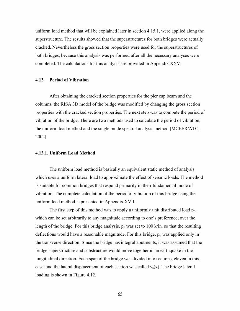
case, and the lateral displacement of each section was called vs(x). The bridge lateral

loading is shown in Figure 4.12.

66

Then the bridge lateral stiffness (K) and total weight (W) were calculated by

using equations 4-1 and 4-2.

MAXs

o

v

LpK

,

= (4-1)

L = total length of the bridge

vs,MAX = maximum value of vs(x)

K = 22601 k/in. for the WB bridge

K = 44045 k/in. for the EB bridge

∫= dxxwW )( (4-2)

w(x) = weight per unit length of the dead load of the bridge superstructure and

tributary substructure

W = 1515 kips for the WB bridge

W = 1897 kips for the EB bridge

Figure 4.12. The uniform lateral loading on the bridge.

67

gK

WT π2=

g = acceleration of gravity = 386 in/sec2

T = 0.0828 sec. for the WB bridge

T = 0.0664 sec. for the EB bridge

[MCEER/ATC, 2002].

4.13.2. Single Mode Spectral Analysis Method

The primary difference between this method and the uniform load method is that

the equivalent lateral earthquake forces for this method are not uniformly distributed

loads over the length of the bridge. Instead, they are of variable magnitude over the

length of the bridge, as explained later in section 4.15.2. The complete calculation of the

period of vibration using the single mode spectral analysis method is presented in

Appendix XVIII.

As in the uniform load method, first the bridge was subjected to a uniform load po

of 100 k/in, and the resulting deflection of each of the eleven sections as given by RISA

3D was called vs(x). Then the α, β, and γ factors were calculated as follows:

∫= dxxvs

)(α (4-3)

∫= dxxvxws

)()(β (4-4)

∫= dxxvxws

2)()(γ (4-5)

w(x) = the weight of the dead load of the bridge superstructure and tributary

superstructure.

For the WB bridge,

α = 12986 in2

β = 7662 k-in

γ = 63585 k-in2

68

For the EB bridge,

α = 6709 in2

β = 4922 k-in

γ = 21069 k-in2

Then the period of the bridge can be calculated from the expression:

α

γπ

gpT

o

2= (4-6)

T = 0.0708 sec. for the WB bridge.

T = 0.0567 sec. for the EB bridge.

[MCEER/ATC, 2002].

As expected, the periods of vibration obtained by using the uniform load method were

longer than that obtained using the single mode spectral analysis method, because the

uniform load method uses a uniformly distributed load, which is a larger force on the

superstructure in the transverse direction of the bridge, compared to the different

magnitudes of distributed load along the bridge for the single mode spectral analysis

method.

4.14. Design Response Spectrum Curve

After the periods of vibration were determined, the next step is to draw the design

response spectrum curve, from which the spectral acceleration (Sa) can be obtained.

SDS = 0.405 g (computed in section 4.9)

SD1 = 0.118 g (computed in section 4.9)

ondg

g

S

ST

DS

D

Ssec291.0

405.0

118.01

===

To = 0.2 Ts = 0.2 (0.291 second) = 0.0583 second

[MCEER/ATC, 2002].

69

The design response spectrum curve for this bridge is given in Figure 4.13.

0

0.05

0.1

0.15

0.2

0.25

0.3

0.35

0.4

0.45

0 0.2 0.4 0.6 0.8 1 1.2 1.4

Period (T) (sec.)

Sa (

g)

SDS = 0.405 g

0.4SDS = 0.162 g

SD1 = 0.118 g

T0 = 0.0583 sec. T0 = 0.291 sec.

Figure 4.13. The design response spectrum curve for this bridge.

It can be seen from Figure 4.11 that for T = 0.0828 sec. (WB bridge) and T = 0.0664

sec. (EB bridge), Sa = 0.405 g.

4.15. Equivalent Earthquake Forces

After obtaining the spectral acceleration from the design response spectrum curve,

the equivalent earthquake forces were computed. The equivalent earthquake forces can be

computed using the uniform load method and the single mode spectral analysis method

[MCEER/ATC, 2002].

70

4.15.1. Uniform Load Method

The equivalent earthquake force pe was calculated using the expression:

L

WSp a

e= (4-7)

Sa = the spectral acceleration from the design response spectrum curve

[MCEER/ATC, 2002].

For the West Bound bridge, pe = 0.262 k/in., and for the East Bound bridge, pe =

0.327 k/in. The complete calculation of the equivalent earthquake force using this method

is provided in Appendix XVII.

4.15.2. Single Mode Spectral Analysis Method

As explained briefly in section 4.13.2, the equivalent earthquake force computed

using this method is not a uniformly distributed load as in the uniform load method. The

equivalent earthquake force pe was calculated using the expression:

)()()( xvxwS

xps

a

e

γ

β= (3-8)

pe(x) = the equivalent earthquake force for that section

Other variables as defined in section 4.13.2.

[MCEER/ATC, 2002].

Since each span of the bridge was divided into eleven sections and each section of the

span had a different deflection vs(x), each section also had a different equivalent

earthquake force. Thus the equivalent earthquake loading for the bridge using this

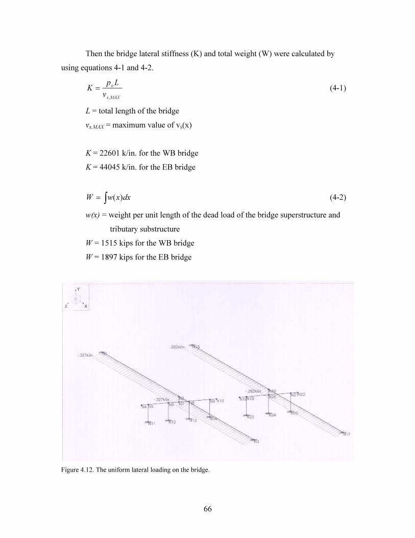
method looks like that shown in Figure 4.14 and 4.15. The distributed load in the middle

is much larger than the other distributed loads, because the distributed load in the middle

carries the tributary load of the substructure. The complete calculation to compute the

equivalent earthquake force using this method is presented in Appendix XVIII.

71

4.16. Combined Effects of the Dead, Live and Earthquake Loads

The final analysis of the bridge was performed using the cracked section

properties for dead, live and earthquake loads. The procedure to calculate the dead and

live load effects for this final analysis is the same as when performing the analysis to

calculate the dead and live load effects to obtain cracked section properties, which was

explained earlier in sections 4.6 and 4.7. For the earthquake loads, the axial loads,

Figure 4.14. The segmentally uniform loading of the West Bound bridge

72

Figure 4.15. The segmentally uniform loading of the East Bound bridge.

moments and shears for the pier cap beam and columns were taken directly from the

analysis on the entire bridge, unlike the dead and live loads, for which a separate

additional analysis had to be performed on the pier structure. The load factors used to

combine the dead, live and earthquake load effects are given in Table 3.4 (Extreme

Event-I), which was shown earlier in section 3.8. But for the earthquake loads, the

responses (axial loads, moments and shears) were divided by the R factor given in Table

3.9. Since SDAP D (Elastic Response Spectrum Method) and the Operational

performance level were used in this research study, the earthquake load responses on the

columns were divided by R = 1.5. Thus the combined effects of the dead, live and

earthquake loads are given by this expression:

++=

5.10.15.00.1

EQLLDLP (4-9)

The complete results of the dead, live and earthquake load effects are given in Appendix

XIX.