Live long and Prosper! - UAB Barcelona · 2015. 2. 28. · the lovely Aram . Thanks, thanks a lot. Thanks also Gustavo and Alexandra, my great friends, thanks for your patience with

Live long and Prosper!Departament d’Arquitectura de

Computadors i Sistemes Operatius

Live long and Prosper even more!!!

Performance Evaluation of Applicationsfor Heterogeneous Systems by means of

Performance Probes

Thesis submitted by Alexandre OttoStrube for the degree of PhilosophiaeDoctor by the Universitat Autonoma deBarcelona, under the supervision of Dr.Emilio Luque

July 15, 2011

Preface

Memoria presentada por Alexandre Otto Strube para optar al grado de Doctor porla Universidad Autonoma de Barcelona. Trabajo realizado en el Departamento deArquitectura de Computadores y Sistemas Operativos de la Universidad Autonomade Barcelona dentro del programa de Doctorado en Computacion de Altas Presta-ciones bajo la direccion del Dr. Emilio Luque Fadon.

4

“I almost wish I hadn’t gone down that rabbit-hole

-and yet-and yet-

it’s rather curious, you know, this sort of life!”

— Alice in Wonderland

Acknowledgments

This is a strange part of this work. One is always afraid of saying the old cliches, orof forgetting to mention some person and then, unwittingly, hurt someone’s feelings.At least I don’t care about the cliches.

Before anything, some unusual acknowledgments: mr Carlito Jensen, a goodfriend of my dad. Why? Because I have stolen I book of COBOL from his housewhen I was less than five years old. That book shaped my life like nothing else did.My cousin Ricardo, who started teaching me BASIC when I was 6, and d.Neda, whokept on my education on computers during primary school, when my colleagues weretrying to learn how to subtract, and who hired me as a teacher for the computingscience classes when I was 12.

Let’s get started. First and foremost, Andrea “Dolly” Couto, my old friend,versed in pretty much anything, from languages to art, cooking, photography, sailing,beer and wines to software system analysis. She started the chain of events thatmade me start in a Ph.D., and without her, I would not be here at all. I don’t knowif I should thank you or smack you, but I prefer the former. So I pay for the beer!

Then Eduardo, who was of more importance than he probably knows about.Besides his help on my first steps as a researcher, his thesis was the whole base ofmy work. I try to mimic - mostly unsuccessfully - his discipline and writing style,in the sense of completeness and cohesion. Thanks Edu.

In Computer Science, every work tends to be radically different from the pre-vious one. My personal guru from the very first moment I landed in our lab, Genarohelped me with his seemingly infinite knowledge of everything related to computersand other subjects, and with his good will to everyone. Again, I could not havedone this without you, my friend.

Of course I cannot forget to thank Emilio Luque and Dolores “Lola” Rexachs.Your wisdom, patience and care go far beyond research. You are not only my rolemodel as researchers, but as human beings. One day I aspire to be like you.

I cannot forget my sister Fernanda. She has a heart as big as my parents, and

a smile as beautiful as the sky. And she gave me my niece, Gabi, which I see duringthese lonely and long nights working. She is the piece of hope that this world canbe a better place.

As we are in the subject of people I aspire to be like, I cannot forget myparents, Ralf and Nilce. I have no words to explain how I love and admire you.If one day I manage to be half the human being you are, I will be a great personalready. Thanks for everything, always.

Pretty much no one is quite sure about the existence of a god, but one thingI know for sure: guardian angels exist. Some of them helped me directly. See, myhealth has not been the best during these crazy years. But when my heart decidedto give a break to tell me to go slower, Hisham was on my side all the way to thehospital. Would I be here if it were not for him? Probably no.

Likewise, when the anaphylaxis hit me like a tsunami, letting me blind andwith a start of a cardiac arrest, Katia literally dragged me to the doctors. Shehelped in so many ways throughout the years that I can only say thank you. I hopeyou are happy, wherever you are.

In a large journey like this, from an arrogant grad student to a humble Ph.D,you never go alone. Dario, the brother I discovered in this side of the world, alwayshad the shoulder and the ears available when I needed, and for bringing to the worldthe lovely Aramı. Thanks, thanks a lot. Thanks also Gustavo and Alexandra, mygreat friends, thanks for your patience with this crazy friend. And thanks Danieland Jamile. I spent almost as much time in their house as in mine. They made thedistance from my family a little more bearable, by putting me into theirs.

Being this a small world, I have had the opportunity to make a friend in somany different places and circles that it is hard to be just coincidence. From thetimes when we both worked on internet providers, then to the motorcycling world,then to the sailing world, and finally, working side by side 10.000km far from wherewe met, I must thank Leonardo for being such an example of worker I should be,and of living to the full and surviving to it.

My second family supported me and has set the example of how someone frommy generation can be happy and good. Thanks Kathrine, thanks Charles, thanksmy godson Oscar, thanks Ricardo.

Thanks Carla, and thanks Luciano, for the wii matches, for all the fun andjoy.

I must say thanks, or “multumesc”, to my great friend Alex Prunean. Weboth have been through difficult times, and you helped me a lot. I hope I did, too.

I cannot forget my colleagues students, some who started with me, some who

were there already, and some who came later: Alvaro Wong, Chris, John, Alex,Pilar, Claudia, Gonzalo, Moni, Ihab, Jairo, Alvaro Chalar, Ronal, Andres, Tharsoand others which deserve to be here as well.

After I left Barcelona, life turned another way, and new people, new experiencesentered into my life. I must thanks all the support from my new bosses, Felix andMarkus, and from my colleagues and now friends, Pavel, Micha, Claudia, David,and Peter.

Last, but not least, the person who is saw how hard these last steps of the Ph.D.have been, and who is making my days sunnier. Olga, thanks for your patience, yourcare and your love.

Contents

Preface 3

Contents i

1 Introduction 1

1.1 Some history . . . . . . . . . . . . . . . . . . . . . . . . . . . . . . . 4

1.2 Objectives . . . . . . . . . . . . . . . . . . . . . . . . . . . . . . . . . 5

1.3 Proposal and Outcomes . . . . . . . . . . . . . . . . . . . . . . . . . 5

1.4 Related Work . . . . . . . . . . . . . . . . . . . . . . . . . . . . . . . 6

1.5 Work Organization . . . . . . . . . . . . . . . . . . . . . . . . . . . . 8

2 The multi-cluster environment 9

2.1 Introduction . . . . . . . . . . . . . . . . . . . . . . . . . . . . . . . . 9

2.2 The free ride . . . . . . . . . . . . . . . . . . . . . . . . . . . . . . . . 9

2.3 Clusters of workstations . . . . . . . . . . . . . . . . . . . . . . . . . 10

2.4 The master/worker paradigm . . . . . . . . . . . . . . . . . . . . . . 10

2.5 Multi-clusters . . . . . . . . . . . . . . . . . . . . . . . . . . . . . . . 11

2.6 The hierarchical multi-cluster . . . . . . . . . . . . . . . . . . . . . . 12

3 Basic Block Vector Distribution Analysis 17

3.1 Introduction . . . . . . . . . . . . . . . . . . . . . . . . . . . . . . . . 17

3.1.1 Metrics . . . . . . . . . . . . . . . . . . . . . . . . . . . . . . 17

3.2 Basic Block Vector Analysis . . . . . . . . . . . . . . . . . . . . . . . 19

i

4 Probe 25

4.1 Introduction . . . . . . . . . . . . . . . . . . . . . . . . . . . . . . . . 25

4.2 The alternatives . . . . . . . . . . . . . . . . . . . . . . . . . . . . . . 26

4.2.1 Thorough executions . . . . . . . . . . . . . . . . . . . . . . . 26

4.2.2 Comparison of hardware characteristics . . . . . . . . . . . . . 26

4.2.3 Benchmarks . . . . . . . . . . . . . . . . . . . . . . . . . . . . 27

4.3 Our alternative: the Probes . . . . . . . . . . . . . . . . . . . . . . . 28

4.4 Creation methodology . . . . . . . . . . . . . . . . . . . . . . . . . . 30

4.4.1 Overview . . . . . . . . . . . . . . . . . . . . . . . . . . . . . 31

4.5 Data Collection . . . . . . . . . . . . . . . . . . . . . . . . . . . . . . 33

4.6 Phase discovery . . . . . . . . . . . . . . . . . . . . . . . . . . . . . . 35

4.7 Binary generation . . . . . . . . . . . . . . . . . . . . . . . . . . . . . 36

4.8 Probe execution . . . . . . . . . . . . . . . . . . . . . . . . . . . . . . 37

4.8.1 Phase save . . . . . . . . . . . . . . . . . . . . . . . . . . . . . 38

4.9 Measurement . . . . . . . . . . . . . . . . . . . . . . . . . . . . . . . 39

4.10 How it fits in the multi-cluster model . . . . . . . . . . . . . . . . . . 42

5 Reduced Probe 45

5.1 Introduction . . . . . . . . . . . . . . . . . . . . . . . . . . . . . . . . 45

5.1.1 Memory access pattern . . . . . . . . . . . . . . . . . . . . . . 45

5.1.2 Program control flow . . . . . . . . . . . . . . . . . . . . . . . 46

5.2 Reduction . . . . . . . . . . . . . . . . . . . . . . . . . . . . . . . . . 47

5.3 Removal of less-important phases . . . . . . . . . . . . . . . . . . . . 47

5.4 Compression . . . . . . . . . . . . . . . . . . . . . . . . . . . . . . . . 50

5.5 Touched set approach . . . . . . . . . . . . . . . . . . . . . . . . . . . 50

5.5.1 Probe generation . . . . . . . . . . . . . . . . . . . . . . . . . 51

5.5.2 Checkpointing library kernel module . . . . . . . . . . . . . . 52

6 Experimental study 59

6.1 Introduction . . . . . . . . . . . . . . . . . . . . . . . . . . . . . . . . 59

6.2 Experimental results . . . . . . . . . . . . . . . . . . . . . . . . . . . 60

6.2.1 Precision . . . . . . . . . . . . . . . . . . . . . . . . . . . . . . 62

6.2.2 Probe Transmission Time . . . . . . . . . . . . . . . . . . . . 63

6.2.3 Reducing Probe size . . . . . . . . . . . . . . . . . . . . . . . 64

7 Conclusion and future work 73

7.1 Work contribution . . . . . . . . . . . . . . . . . . . . . . . . . . . . 73

7.2 Publications . . . . . . . . . . . . . . . . . . . . . . . . . . . . . . . . 74

7.3 Future Work . . . . . . . . . . . . . . . . . . . . . . . . . . . . . . . . 74

Bibliography 76

Abstract

This doctoral Thesis describes a novel way to select the best computer node out ofa pool of available potentially heterogeneous computing nodes for the execution ofcomputational tasks. This is a very basic and difficult problem of computer scienceand computing centres tried to get around it by using only homogeneous computeclusters. Usually this fails as like any technical equipment, clusters get extended,adapted or repaired over time, and you end up with a heterogeneous configuration.

So far, the solution for this, was:

• To leave it to the computer users to choose the right node(s) for execution, or

• To make extensive tests by executing and measuring all tasks on every typeof computing node available in the pool. In the typical case, where a largenumber of tasks would need to be tested on many different types of nodes, thiscould use a lot of computing resources, sometimes even more than the actualexecution one wants to optimize.

In a specific situation (hierarchical multi-clusters), the situation is worse, asthe configuration of the cluster changes over time, so that the execution tests wouldhave to be done over and over, every time the configuration of the cluster is changed.

I developed a novel and elegant solution for this problem, named ”PerformanceProbe”, or just ”Probe”, for short. A probe is a striped-down version of a compu-tational task which includes all important characteristics of the original task, butcan be executed in a much shorter time (seconds, instead of hours), is much smallerthan the original task (about 5% of the original size in the worst cases), but allowsto predict the execution time of the original within reasonable bounds (around 90%accuracy).

These results are very important: as scheduling is a basic problem of computerscience, these results cannot only be used in the setting described by the thesis (ofsetting the right compute node for tasks in a hierarchical multi-cluster), but canalso be applied in many different contexts every time scheduling and/or selection

decisions have to be made: selecting where a computational task would run mostefficiently (which cluster at which centre); picking the right execution nodes in alarge complex (grid, cloud), workflows and many more.

Chapter 1

Introduction

Read the directions and directly you will be directed in the right direction.— Doorknob

Applications are the reason people use computers. Different applications usethe computers in different ways, and might be better suited to run in one type ofcomputer than another. And yet, as obvious as it should be, to determine the bestmatch between a kind of computer and an application is neither easy nor a solvedproblem at all.

When applications started to become so demanding that a single computerwould not be able to run them in reasonable time, one of the solutions was to joinseveral computers together and divide the problem tackled by these application intosmaller pieces, enough for each computer to process them in a reasonable time. Thecluster was born.

The end of speed improvements in processor cores by simple clock speed in-crease made the evolution go towards adding more computers together to addressthe increasing demand in computing power first, and then adding more processorsinto a single computer, and subsequently adding more cores into a single dye. Apersonal computer of today is not so different from a cluster from yesterday.

Increasing the number of computing elements does not bring automatic im-provements to applications. Applications must be either adapted to conform to thisnew model or rewritten.

One of the most popular models to make an application avail the extra com-puting power provided by multiple computers running together in a network is theMaster/Worker paradigm. A simple definition of it is that a “master” machine as-signs tasks to “workers”, which receives them, compute and return the final resultof this task back to the master. The master will give the workers more tasks untilthe complete problem is solved, and then the master aggregates the results of all

1

2 CHAPTER 1. INTRODUCTION

completed tasks in form of the final result. It is widely used because of its simplicity,reliability and elasticity.

An economic-wise form of having huge computing power is that of clustersof commodity workstations. They are cheap and in case of failures or upgrades,it is easy to replace them individually. It is a system widely used in academia, forinstance, when laboratories might provide the workstations for normal use during theday for students and let them available for parallel applications during non-workinghours.

The replacement cycle of these clusters makes them heterogeneous throughouttime. And as already said, different applications perform differently according to thecomputer where they are running. The heterogeneity also introduces inefficienciesinto the scheduling, which can be seen as times when the workers stay idle waitingfor more data.

This makes the decision of choosing which machine should run a given taskmore difficult.

Clusters of workstations cannot grow indefinitely, be it because of space con-straints, network addressing or even power consumption. Therefore, in order tokeep increasing the computing power to handle ever-increasing problems, one of thesolutions is to add another level in the distribution, by joining multiple clusters ofworkstations together. We call this extra level “multi-cluster”. The Grid and theCloud are specializations of this concept.

The extra level of organization leads to differences in network performances:each cluster has its own high-speed network, but communication between them is notnecessarily (and probably never is) the same. The heterogeneity between machinesis even more probable.

It is worth noting that we call heterogeneous machines and clusters in terms ofinternal architecture or computational power. It does not mean heterogeneity suchas that mentioned in other papers related to GPU or accelerators, for instance.

One form of organizing a multi-cluster running a master-worker applicationis hierarchically. Similarly as a single cluster running a master-worker application,one element acts as a master, while others act as workers. On this case, a mastercluster has not only its own machines to send tasks, but also other clusters. Theseclusters can be seen by the master as machines capable of processing a lot of tasks,but with a higher time required to send tasks to them. The master cluster sends thetasks to a worker, or sub-cluster through an entity called Communication Manager,responsible only for taking care of the communication between a master clusterand its sub-clusters. On the sub-cluster there is another Communication Manager,which receives the tasks and send to a local master, which finally assigns them to

3

individual computing units or even to sub-clusters. This sub-master joins togetherthe results of the tasks under its responsibility, and sends them back to the mastercluster, again using the Communication Manager.

The hierarchical multi-cluster is a powerful tool to handle big problems withadvantages akin to that of a cluster of workstations: it is relatively cheap, simple toimplement, easy to grow, and simple to replace or disable individual elements (oreven whole clusters).

Ideally, machines should be computing as much as they possibly could, withno time lost by waiting between the end of one task and the beginning of the nextone. In order to achieve this, the communications should occur while the workersare computing. So while the worker is computing its task, it should be alreadyreceiving the next one, effectively “hiding” or “masking” the communication time.

Easier said than done. To be able to mask communications, the master ma-chine assigning all tasks must have knowledge of two things:

• The time required to send a given task to each of them. The master shouldsend tasks early enough that a worker wastes no time receiving it, but not soearly that in the case of a malfunction or a slow machine that unbalances thisscheduling, and, of course,

• the computing power of each machine while running this specific application.

These two parameters, network and machine performance are enough for ascheduler to optimize the execution of an application in this hierarchical multi-clusterenvironment. The relationship CPU power/Network bandwidth gives the schedulerknowledge enough to send more tasks to a given machine than another, less tasks, oreven discard a machine (or a whole cluster) completely, either because the machinesare so slow that they does not help at all, or does not help on the efficiency thresholdset, or because the time required to send tasks to them might delay the wholeexecution. The model is able to adapt to changing network conditions throughoutexecutions, and with our Probes, also is able to quickly characterize nodes thatmight become available during the execution.

It is trivial to calculate network performance by just sending data from onemachine to another and calculate the time required to send it. But to determinethe performance of a computer while running an application is a harder task.

Performance characterization and prediction has been a subject in ComputerScience since its inception, and it is an issue far from solved, given the very na-ture of applications and how they run on different computers. Compilers, run-timeenvironments, abstraction layers and virtual machines (such as 1960’s VM, 1970’sCP/M, 1990’s Java and modern full-OS VMs) made the matters even more difficult.


One of the issues of performance characterization has to do with the time takento run an application. If an application is important enough to be characterized, itprobably also tends to have a large execution time, with orders of magnitude fromhours to months, and will be run thousands of times, and these are applications thatrun several times.

The other issue is that different machines behave differently, even though theyare computationally equivalent (or ISA-equivalent) - that is, with the same inputsand the same application, they give the same results, even though the internals arenot identical. Even when machines are apparently the same, smaller revisions ofprocessors or memory controllers can add to heterogeneity.

1.1 Some history

To deal with the issue of execution time, computer scientists came up with theidea of benchmarks. Some of them were totally artificial, created to stress specificcomponents of the computers, while others are kernels of “real” applications withsome fixed inputs, intended reproduce this application’s behavior during a shorttime.

Both kinds of benchmarks can be useful in some contexts - they give people away to compare different computers. The Linpack benchmark [18], for instance, isthe official standard of the Top500 supercomputer ranking [1], and has been usedfor decades as such.

However, benchmarks, as any computer program, only do what they are toldto, and nothing more. The aforementioned Linpack, for instance, criticized for notfulfilling its basic purpose of real comparisons between modern supercomputers, asit does not takes into account the ever-increasing problem of memory-bound codes[90], [77], not being representative even of its own field of dense linear algebraapplications [26], does not represent behavior of applications in general [75], andhave a much higher peak efficiency than real applications [76]. In fact, doubling theLinpack index can give real applications a speedup of only around 10% [53]. So wecan affirm that benchmarks are not useful, per se, as valid tools for performancecharacterization of real applications on computers.

There is research about using micro benchmarks to stress specific computercomponents [21], as they are relatively simple and can be highly optimized for specificuses. Some researchers also join multiple ones together in order to try to correlatetheir performances to that of real applications [39], [43], [64], [40], or even generalcharacteristics of programs [36].

If a computer system is going to be used for a very specific application, there

1.2. OBJECTIVES 5

is no benchmark better than running the application itself. However, suppose thefollowing scenario: a company has this very specific application, that takes weeksto execute every single time. The process of evaluating new equipment to runthis program should evidently stress the characteristics necessary for this specificexecution. With multiple options available, the production of performance indexescan take a time so long that it might be impossible to do it.

There are other scenarios where a precise and quick knowledge of one appli-cation’s performance is desired, as the multi-cluster mentioned before, and that iswhy we pursue the goal of characterizing the performance of a program quickly.

1.2 Objectives

The objective of this work is to create a way to characterize and predict the perfor-mance of one specific part of a parallel master-worker application: the worker, asaccurately and quickly as possible.

The quality of this prediction must be as close to the application itself aspossible, to better inform the scheduler about the performance of each machineavailable in the multi-cluster system. A scheduler must be fast, which means thatthis characterization must be quick, on the order of seconds.

As the multi-cluster environment usually uses slow networks as its intercon-nect, amount of data required to perform this characterization must be reasonable,to be transferred quickly.

These requirements made us create a methodology to analyze an application’sexecution, extract its relevant behavior, shrink it to its bare minimum and build aProbe from it to be sent to the remote machines.

1.3 Proposal and Outcomes

We proposed the creation of a methodology that is able to take a parallel applica-tion’s worker - that is, its serial component, extract its performance characteristics- which means, the phases able to characterize performance, and create a Probe,able to be sent to remote clusters and quickly characterize the performance of everycomputing node available.

This Probe must have a high prediction quality related to the execution timeof the program it originated from, but with a much shorter execution time than it.

The Probe must also be small enough to be transported through slower non-


local networks, such as the internet, in a reasonable time.

Our method basically analyzes the behavior of an execution of the programto be characterized, extracts the non-repetitive behavior from the application andis able to run only the unique behavior, with the repetitions being extrapolatablefrom them.

I think this proposal was reasonably fulfilled. Our Probe methodology is ableto:

• run entirely in three orders of magnitude less time than running the applicationitself,

• predict execution time of the application with an average precision of over90%, and

• be transported through the internet in matter of seconds.

1.4 Related Work

The work of Sherwood, Sair and Calder [66] is one of the foundations of this research.They created a methodology to find repetitive behavior on applications so they areable to reduce run-time for benchmarking future processors on functional simulators.

Further, Sherwood, Sair and Calder [66] proposed a profiling technique ableto understand an execution as a series of different phases that may repeat.

A work related to ours is that of Sodhi and Subhlok [73], where their perfor-mance skeletons intend to mimic application behavior in a shorter execution timefor evaluating shared resources using a node selection algorithm [81]. While theyfocus on shared resources and network usage, we focus this work on computation formaster/worker applications by characterizing the worker. This happens for two rea-sons: (a) it is the model most widely used by cloud and grid environments becauseof the easy ’elasticity’ of it, and (b) our research group already have ongoing workon characterizing communication patterns, such as the study conducted by Wong,Luque and Rexachs [91]. Besides, the general workflow paradigm is composed ofnodes in graphs that only communicates in the beginning and the end. In thissense, a node in a directed acyclic graph (DAG) is no different from a worker. [72][74]

The work of Weaver and McKee [87] developed a tool that runs under theQEMU emulator or the Valgrind as a method to gather multi-platform basic blockvectors faster than when using functional simulators, but to use them inside those

1.4. RELATED WORK 7

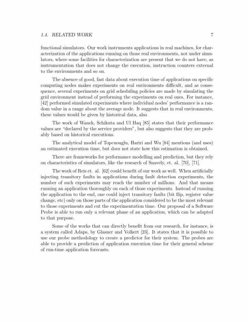
functional simulators. Our work instruments applications in real machines, for char-acterization of the applications running on those real environments, not under simu-lators, where some facilities for characterization are present that we do not have, asinstrumentation that does not change the execution, instruction counters externalto the environments and so on.

The absence of good, fast data about execution time of applications on specificcomputing nodes makes experiments on real environments difficult, and as conse-quence, several experiments on grid scheduling policies are made by simulating thegrid environment instead of performing the experiments on real ones. For instance,[42] performed simulated experiments where individual nodes’ performance is a ran-dom value in a range about the average node. It suggests that in real environments,these values would be given by historical data, also

The work of Wanek, Schikuta and Ul Haq [85] states that their performancevalues are “declared by the service providers”, but also suggests that they are prob-ably based on historical executions.

The analytical model of Topcuouglu, Hariri and Wu [84] mentions (and uses)an estimated execution time, but does not state how this estimation is obtained.

There are frameworks for performance modelling and prediction, but they relyon characteristics of simulators, like the research of Snavely, et. al. [70], [71].

The work of Reis et. al. [62] could benefit of our work as well. When artificiallyinjecting transitory faults in applications during fault detection experiments, thenumber of such experiments may reach the number of millions. And that meansrunning an application thoroughly on each of those experiments. Instead of runningthe application to the end, one could inject transitory faults (bit flip, register valuechange, etc) only on those parts of the application considered to be the most relevantto those experiments and cut the experimentation time. Our proposal of a SoftwareProbe is able to run only a relevant phase of an application, which can be adaptedto that purpose.

Some of the works that can directly benefit from our research, for instance, isa system called Adaps, by Glasner and Volkert [23]. It states that it is possible touse our probe methodology to create a predictor for their system. The probes areable to provide a prediction of application execution time for their general schemeof run-time application forecasts.


1.5 Work Organization

This manuscript is organized as follows. In chapter 2, the environment and program-ming model is described. Chapter 3 sets the theoretical basis for the model. In 4 theapplication characterization method and the Probe construction is described, wherechapter 5 goes a step further, into the description of methods to reduce Probes’sizes. Chapter 6 is the experiments and results chapter, and this work is finished inchapter 7.

Chapter 2

The multi-cluster environment

Let me see: four times five is twelve, and four times six is thirteen, and four times sevenis – oh dear! I shall never get to twenty at that rate! — Alice

2.1 Introduction

For decades, the advances in raw computing processing power has been given byfaster chips, with more transistors per chip, and faster clock speeds. The number oftransistors per chip approximately doubled every 18 months, which was predictedby Intel’s co-founder Gordon Moore in 1965. Since then, this computing powerexponential increase has been known as Moore’s Law.

2.2 The free ride

Programmers, however, called it differently: “the free ride” [82]. The simplest wayto make your program faster was to simply wait for the next generation of processors,and with no additional effort from the programmer, her application would run faster,“for free”.

Even though algorithms able to process data in parallel exists for years [69],programmers kept taking advantage of the free ride for as long as possible - whichmakes sense. Why bother in learning new (and recognizedly difficult) techniquesthat most computers would not be able to extract any advantage at all?

The exponential growth of computing power, however, reached two relatedobstacles: power consumption and heat dissipation. The more power a processoruses, the more heat it generates. The added heat needs more dissipation, which in

9

10 CHAPTER 2. THE MULTI-CLUSTER ENVIRONMENT

turn also consumes more power.

2.3 Clusters of workstations

With the advent of local-area networks, a form of computing became readily and,most important, cheaply available: the clusters of workstations (COWs). Linkingtogether several computers into a network and making them work towards the so-lution of a single problem is one of the most cost-effective ways to tackle problemsbigger than the capacity of a single computer.

Scientific computing has changed a lot in the last decades. From the vectorcomputers of the past, to personal academic workstations, the current trend is toaggregate a big number of processing units by means of one or more interconnects,in the form of clusters. Today, every supercomputer is built around the principle ofaggregating a number of CPUs ranging from the dozens to hundreds of thousands,each with relatively small computing power, where applications run in parallel in allthese processing units, in order to achieve a single goal, be them highly specializedmachines, or if they are small clusters of standard workstations interconnected byethernet networks.

Most of highly specialized machines, such as the modern supercomputers, usesproprietary interconnects, homogeneous CPUs and its own I/O, cooling systems,etc. On the other hand, clusters of standard workstations tend to be heterogeneousby nature, even when the machines share a common ISA and operating system -be it by the multiplicity of vendors and platforms, be it by the natural replace-ment cycle of machines. Heterogeneity, even in single clusters, brings hindrances toparallel programming: scheduling, load balancing, domain decomposition, processorselection, as mentioned by [15].

2.4 The master/worker paradigm

The textbook example of parallel programming is the master/worker paradigm.On it, the computation and the data are divided in tasks that can be executedindependently and simultaneously on different computing elements.

On it, two distinct entities exist: one master and some workers. The master isresponsible for decomposing a problem into tasks, and for distributing these tasksamong its workers. Also of masters’s responsibility is to gather the results fromthese workers and from them, generate the program’s final output.

The workers operate cyclicly: they receive the task, process it and the result

2.5. MULTI-CLUSTERS 11

back to the master, and wait for the next task.

The great advantage of the master/worker paradigm is that it is well-suitedfor dynamic, heterogeneous environments, where adaptability, reliability, capabilityand efficiency are required [25].

• Adaptability, or elasticity: the same program can be solved in different envi-ronments, with different number of workers, and even with changing numberof workers available, when allowed by the runtime. The performance increasecan be made by adding more workers;

• Reliability: the loss of one of more workers during an execution affects onlythe execution of the task being computed by the element lost. The overallfunctioning is not affected;

• Capability: more powerful computing elements will finish performing theirtasks before other elements; In the master/worker model, it will simply “ask”for more work, instead of waiting for some synchronization barrier, for instance;

• Efficiency: computing elements must not be idle waiting for others. Idle timesin single units add to the overall execution time. We understand efficiencyhere as the time the computing elements are effectively working in proportionto the total execution time - that is, excluding the moments they are idle.

These factors are essential, for instance, in cloud computing environments,where the number of computing elements and their computing power is highly vari-able among executions and possibly even during one specific execution. It is alsoessential for grid environments, where the available computing elements for perform-ing a computation are not usually known beforehand and might have some dynamicchanges in the environment throughout the execution.

2.5 Multi-clusters

A natural extension of the act of gathering machines together in the form of thecluster is that of joining clusters of workstations together. The ample availabilityof network connectivity across organizations and the pervasiveness of the Internetmade possible the creation of these multi-clusters.

There are several forms of multi-cluster, from the simple act of using a set ofgeographically distributed machines that can communicate directly to each other,to grids, most present in scientific research, and cloud environments, popular amongenterprises.


However, the usage of multi-clusters to increase computing power brings withitself added levels of heterogeneity, and with it, further difficulties in schedulingand processor selection [50]. Now, not only the heterogeneity between machines isimportant, but the heterogeneity in terms of interconnect of each cluster, the inter-connect between clusters and heterogeneity in computing power among individualnodes are important. The communication between each pair of clusters might bedifferent, and this poses a challenge for masking the communication time throughoutthe computation.

Heterogeneity between machines is a well-studied problem[84] [57], but inmulti-clusters, efficient executions of applications is field less touched.

These factors are not linear and worse, not uniform across applications. Whatis perceived as an inferior CPU for one application might not be the case for anotherone. Differences in cache usage, for instance, account for big differences in applica-tion performance, and the same happens for every other parameter that influencesin performance.

2.6 The hierarchical multi-cluster

The hierarchical multi-cluster is a extension of both concepts of geographically dis-tributed multi-cluster and the master/worker paradigm. In this architecture, eachcluster is a master/worker itself. The cluster where the application is launched isconsidered then the master cluster. The other ones are called sub-clusters, and in-side them there are the figures of the sub-master, the sub-workers. On all clusters,the element responsible for managing WAN communication is the CommunicationManager (CM), as seen in figure 2.1

In this scheme, what the master node sees is a set of machines where it cansend tasks to. The CM then is responsible to send tasks to the sub-clusters underits responsibility and receive computation results from them. In that sense, whatthe master perceives is that the CM behaves like a powerful machine (given it is thecomputing power of its sub-clusters) with a higher interconnect latency (because itis sending tasks to its sub-clusters through the internet).

This architecture allows great flexibility and scalability to run master/workerapplications, as to increase computing power is a matter of adding more clusters, aslong as the interconnect allows it.

As the sub-clusters are seen by the master node of the master cluster as apowerful node, it might send tasks of either coarse-grained or more tasks, in thecase of a fixed-sized problem. To optimize communication, the CM might makeuse of a pipeline scheme in order to send and receive a higher amount of work to

2.6. THE HIERARCHICAL MULTI-CLUSTER 13

Sub-Master

Sub-Master

Sub-Master

Master

CM

CM

CM

Master cluster

Subcluster A

{Workers

Subworkers

Subworkers

SubworkersSubcluster B

Subcluster CInternet

CM

Figure 2.1: A hierarchical multi-cluster environment. Different machine sizes repre-sent different processing power. Thickness of the arrows represent different networkbandwidths.


a sub-cluster than that which would be sent to a single worker, and make use ofbuffers/caches to communicate only when necessary.

Sub-masters receive work from the master cluster via communication manager.They then behave as regular masters in single clusters. They can schedule their tasksand grain sizes among their workers, and join back the results to send back to themaster cluster.

Workers and sub-workers work identically - they receive tasks from a master- be it the root master or from their own master, compute it, send the results backto their master, and request new data. In order to mask communication time, theymight start receiving the next task in background before they finish their currenttask, and can send their results back to their master while already processing itsnext task.

On the application level, the communication manager and the sub-clustersare transparent, so it can be run unchanged in a single cluster or in a hierarchicalmulti-cluster, and even with failures in communicating with the sub-clusters, as theCM is able to detect it and redistribute the work accordingly, without stopping theapplication.

The work of [9] sets the basic ground for this work. On it, an analytical modelfor execution of master/worker applications in hierarchical multi-clusters is defined,based on the CPU and network performances between the different elements andthe computation/communication ratios.

This model is able to run master/worker applications on a set of aggregateclusters working together hierarchically, and the cluster where the application waslaunched sees the other clusters as powerful machines, with usually slower networksthan its own nodes. According to this power to bandwidth ratio, this model candecide on the number of tasks to send to the sub-clusters, to use only parts of themor slash clusters entirely, if they will not be able to reduce this application computingtime over a user-specified efficiency threshold.

This model is also able to predict a master/worker application execution time.But both for scheduling the number of tasks and for predicting total execution time,two kinds of information are required:

• The network throughput between all the clusters, and

• Computational capacity of every node available, in every cluster, for thatspecific application.

To calculate network throughput is trivial. To calculate computational ca-pacity, however, is not straightforward. The model of [9] actually ran at least one

2.6. THE HIERARCHICAL MULTI-CLUSTER 15

task of the application on every unique available node, during the first step of itsexecution, to then decide where to run.

This, of course, brings its own sort of problems. Very early in my research, Irealized two problems with this model:

• Some nodes (in one of the Universities’ heterogeneous cluster) were so slowthat this performance determination would take an unfeasible time to run,sometimes even longer than the rest of the application.

• The performance results were not valid for the next executions, as it was reallycommon to have different sets of computing nodes in some clusters beyond ourcontrol.

So, basically, the performance estimation was taking an unrealistic time.

Our goal is to enhance the efficiency of master/worker applications on heteroge-neous environments, where the available machines - and, of course, their performance- is not known until the time to run this application comes.

We focus our studies on master/worker applications, but any environmentwith heterogeneous machines that needs quick and precise information about howan application will perform on a given machine may benefit from our method. Thatis, queueing systems that selects resources based on availability, performance andefficiency, such as grids and clouds, can take advantage of this research.


Chapter 3

Basic Block Vector DistributionAnalysis

Speak English! I don’t know the meaning of half those long words, and I don’t believe youdo either!— Eaglet

3.1 Introduction

This chapter explains the base methodology used to find repetitive behavior on anapplication’s execution, made independent from any hardware characteristics. Itis related to how the code performs, although it is totally independent from theprogramming language used and even from the presence of the source code at all.Instead, if focus on how the code’s flow, which is highly correlated to the sourcecode. This methodology is called basic block vector analysis.

3.1.1 Metrics

In order to characterize a program’s execution, metrics are needed. Given we wantto predict execution time, the first metric is, evidently, execution time.

Nevertheless, just execution time is not enough for characterization - and moreimportant, it does not help us find repetitive behavior, which we could trim out fromthe Probes.

The first metric we analyzed was the cache hits/misses of the applications.Considering the ever-growing gap between the processor speeds and memory laten-cies, one access to a memory position not replicated in the first-level cache (a cache

17

18 CHAPTER 3. BASIC BLOCK VECTOR DISTRIBUTION ANALYSIS

miss) might stall the processor for hundreds of clock cycles. So the cache miss/hitratio during an execution, if replicated, could mimic a great part of an applicationprogram.

The obvious issue with the cache hit/miss metric is that it is completely depen-dent on the underlying hardware. Even in hardwares of the same architecture line,different cache sizes or configurations might produce unbeknownst consequences.

Moreover, the cache miss ratio is a metric derived both from the hardware andfrom the behavior of the memory access pattern.

The memory access pattern alone can represent a significant part of the per-formance characteristics of an application [10] , but it is not the panacea that cangive an optimal representation of the execution time, as issues such as address spacerandomization and allocation above the available capacity - which might make thesystem start to make use of virtual memory - makes the memory access pattern aan information of little use for our needs when taken into account individually.

Furthermore - the memory access itself is derived from a more fundamentalbehavior - and this one independent of the specifics of the underlying hardware: thecode itself.

Other researchers arrived to the same conclusion - which bolstered our decisioninto investigating the path of mimicking the program control flow itself.

The program control flow can be described as a series of decisions, jumps andloops. And the structure of programs makes that some behavior repeats itself, suchas a calculation done over a large amount of data, for instance, or a function beingcalled several times.

Although programs have repetitive behavior, on the same time, throughoutexecution they can have wildly different behavior. During one part of an execution,a program can be cpu-bounded, and in a further moment, it can turn to memory-bound as a consequence of a different part of it being run.

The changes into a program’s execution from one state to another tend to re-peat. We call these repetitions phases, and that is one of our basic elements. Phasesare sets of intervals within a program’s execution that present similar behavior,regardless of temporal adjacency [48].

This work classify phases breaking a program into intervals of execution, andfinding similarity between them. Similarity is how close an interval of the programexecution is close to another in some metric. In our case, we classify similarityby the number of executions of each basic block into each interval - that is, eachvector, with the other vectors. Vectors where the more or less same basic blocks areexecuted more or less the same amount of time tend to take the same time to run

3.2. BASIC BLOCK VECTOR ANALYSIS 19

in the large scale.

For classifying similarity, we do not use any architecture, but as already stated,the program’s control flow is used to classify similarity, as what the code is doing ata particular moment determines the program’s behavior.

With this insight, it is possible to find phases in programs without hardware-dependent metrics at all.

The metric used to classify the code traversal throughout the execution is theBasic Block Vector Analysis, explained below.

3.2 Basic Block Vector Analysis

In a well-designed master/worker application, the determinant in execution time isthat of the workers computing their tasks. So we focus our efforts on understandingthe performance of the worker.

Most code that does not depend on constant user iteration (such as majority ofscientific high-performance applications) presents repetitive behavior of some sort -methods and functions calls, and loops, are all repetition of the same code with somedifferent parameters. This is especially true in number-crunching scientific code.According to Sherwood, Perelman and Calder [65], “the large scale of programs iscyclic in nature”. On their research, they measured under simulation that for theSPEC95 benchmarks, the hardware statistics in fixed periods of time, and notedthat these statistics (1) repeat from time to time, or (2) have a repeatable cyclicbehavior until the end of their execution. It is demonstrated that periodicity of thebasic block frequency profile “reflects the periodicity of detailed simulation acrossseveral different architectural metrics (e.g., IPC, branch miss rate, cache miss rate,value misprediction, address misprediction, and reorder buffer occupancy)”.

Periodic behavior is defined as a repeatable pattern seen for a given architec-ture metric. On Sherwood’s breakthrough article, it is possible to notice that nomatter what the hardware characteristic is chosen, they change at the same time,i.e., there are distinct phases, and to discover them, they used a metric indepen-dent of any architectural parameter, but highly correlated with their performance.Their intuition was that what is executed in a given moment determines programbehavior, and it reflects on architectural metrics.

This metric is then given by counting the number of times a piece of code -defined here as basic block - is executed under several contiguous periods of time.This is the most efficient technique for phase detection, according to Dhodapkar andSmith [17]. In this work, fixed-sized phases are used, as they work well enough, but


there is research on phases with variable sizes and even hiearchical ones, such as inthe work of Lau[47]. The size of the phase means the number of instructions of oneor more basic block vectors.

A basic block is classically defined as a piece of code with one point of entryand one exit - i.e. no control flow. They called this metric “basic block distributionanalysis”. A key point is that the phase behavior seen in any program metric isdirectly a function of the code being executed [49, 68] . Because of this, a metricthat is related to the code can describe phase behavior [67].

Sherwood’s goal was to reduce run-time of functional simulators for next-generation processors. With a functional simulator, it was possible to count theinstructions and have precise information of which basic block of a given code thissimulated processor is running.

The biggest insight was the selection of an approach that does not use anyknowledge of the architectural state of a program, but yet is highly correlated withthe performance of such metrics.

His method consisted in counting the number of times a basic block was ex-ecuted during a fixed number of instructions (called the basic block vector - BBV[65]), and compare the similarity of these vectors.

Their goal with such method, for the field of computer architecture simulation,was to find:

• The end of the initialization part of the program, and the start of the cyclicpart of the program.

• The period of the program. The period is the length of the cyclic nature foundduring a programs execution.

• The ideal place to simulate given a specific number of instructions one hastime to simulate.

• An accurate confidence estimation of the simulation point.

Simulation point here means the exact point in the execution where one couldstart the simulation (recovering from an architecture checkpoint, complete withcache/register/memory state, straightforward in a simulator), thus reducing simu-lation time.

It is common that applications pass through a initialization period, where itsdata structures are created, files are created and read and so on, before proceedingto the actual processing phase. The processing phase usually consists of periodic


behavior, alternating between completely different sections of code (functions, pro-cedures, loops, methods).

The idea is that similar vectors were running more or less the same code, and,on large scale, they tend to take the same execution time [61].

By having the same execution time, it was possible to run only a reducednumber of occurrences of one phase, skipping repetitive behavior [59]. This greatlyreduced simulation time. In figure 3.1, for instance, the three dominant functions,x solve, y solve and z solve took the wide majority of this execution’s time, but byno means the functions themselves took a long time, but instead, the sheer numberof calls to these functions.

Their work resulted in a tool, called Simpoint [27]. Basically a K-means clus-tering algorithm that reads a basic block vectors’ file and points out the relevantphases found, to drive the simulation to these specific points. The basic blockswere collected either during functional simulation or in real machines through codeinstrumentation [58] in order to feed the simulator later.

Once an application is profiled, for instance from an execution trace of anarchitecture simulator such as simpleScalar [14], the basic block profile is then fedinto their SimPoint [28] tool.

Our Probe departed from the concept of phase classification and simulationpoints and implemented these in a tool that is able to run in real computers, runningreal code, instead of simulators. The specifics of the Probe are going to be discussedon the next chapters.

Simpoint is a tool that uses the k-means algorithm from machine learningto group code signatures into clusters based on signature similarity. The singlemost representative code signature from each group is selected for execution, theimportance of this selected phase is weighted, and the results of each execution areextrapolated to estimate the program’s overall behavior, according with each phase’sweight.

Each execution phase has a typical set of instructions, that is, under a givenperiod of time the application will use only a subset of the total architecture instruc-tion set. Dhodapkar and Smith found that exists a relationship between phases andarchitecture instruction working sets, and that those phase changes tend to occurwhen the instruction set changes. In [17] they found that BBV analysis is accurate.Their approach focused on online phase classification. On the other hand, Simpointis an offline tool.


0

50000

100000

150000

200000

Jacobi

initialize copy_x_face copy_y_face compute_rhsx_solve y_solve z_solve

Function:

Time(s):

Figure 3.1: Total time spent for the main functions in the Jacobi Relaxation Bench-mark as measured by the Scalasca toolset in 1024 processors.


According to [48], the representatives for each phase selected by Simpoint basedon full-BBV data not only represent the whole program well, but also represents eachphases well. Their results shown an average error rate about 2% on the CPI metricwhen compared with full executions across the SPEC2000 benchmarks.

Their first attempt was to find a single continuous window of executed instruc-tions that matched the whole program’s execution, so that this smaller window ofexecution can be used for simulation instead of executing the program to completion.In [67], Sherwoord, et. al found out that more sophisticated applications cannot berepresented using a small contiguous section of execution.

Applications do have regular behavior, however not in a single window ofexecution, coming from the beginning to some specific point. Instead, the repetitivephases are found along the whole execution of some program. To find them, Simpointexamines the similarity between different phases, grouping the ones which are similartogether, in a method called clustering. The goal of clustering is to divide a set ofpoints into groups such that points within each group are similar to one another,and points in different groups are different from one another.

One problem with the clustering algorithm used in simpoint, the k-means, isthat its performance suffers from the excess of dimensions on the basic block vectors,as every basic block is one dimension across the different BBVs. So the target basicblock vector from the full execution can have millions of dimensions on one fairlycomplex application.

To address this problem, it was used an algorithm dimension reduction, bycreating a new lower-dimensional space and then projecting each data point intothe new space. The algorithm is the random linear projection, that reduces theamount of dimensions while retaining the properties of the data.

In [67], it was found out that 15 dimensions are enough to correctly clusterthe phases, and that increasing this number gives little for improvement on findingclusters. Once the clusters are found, it is necessary to run then, in a noncontiguousway, as they can be spread among the whole execution. That is, the executioncan be broken down into N executions, where N is the number of clusters foundthrough analysis, and each execution is run separately. On homogeneous clusters ofworkstations, this can be used to break the execution into parallel components thatcan be distributed across the nodes. In any case, results from the separate clustersof phases needs to be weighed and combine to arrive at the overall performance ofthe program.


Chapter 4

Probe

What is the use of a book, without pictures or conversations?— Alice

4.1 Introduction

The general idea is that if we are able to know how long will an application taketo run on a machine without taking the time that would be required to run itthoroughly previous to an execution, we will be able to decide if this machine fitsour needs or not.

For that, we came with the concept of a software Probe. We define a Probe as apiece of code that is able to quickly extract useful information about the relationshipbetween the application and the system we want to know about. This means that aProbe from a given application will run fast and will return us precise informationabout how the application we are analyzing is going to run in there.

The work in multi-clusters already introduced at chapter 2, and described inmore detail in [8] , [9] deals with the issue of efficiency of Master/Worker applicationsin those heterogeneous and distributed environments. For it, efficiency is defined asthe ratio between the best possible execution time Tbest and the total execution timeTex, as in equation 4.1:

(4.1) Efficiency =Tbest

Tex

Basically, that means the proportion between the time taken actually doinguseful computational work over the total execution time, with delays.

25

26 CHAPTER 4. PROBE

Several works on the literature uses simulated environments, usually because ofthe long times required to characterize applications and test their policies, as notedin chapter 1. The work of Kim, Rho, Lee and Ko [42] is typical: they performedsimulated experiments where individual nodes’ performance is given by a randomvalue in a range around the average node’s one. It suggests that in real environments,these values could be given by execution historial.

Therefore, the absence of a good and fast way to determine execution timehas hampered experiments on real environments for a long time. Mostly, eitherhistorical data or simulation was used. Until now.

4.2 The alternatives

Before explaining our method, we briefly introduce two of the alternatives, why theycould be useful or otherwise: Thorough executions and Benchmarks.

4.2.1 Thorough executions

The explanation for this one is straightforward: there is no better method to pre-dict the execution time of an application running in a machine than running thisapplication itself. The obvious problem with that is the execution time requiredto do this makes it of little use for the selection of sub-clusters or sets of machinesaccording to the communication/computation rates. Actually, this was the methodused on the multi-cluster environment already which is the base of our research.

The problem is not isolated to the fact that execution time of one worker doingthis first task thoroughly may delay the overall execution, but furthermore, as atleast one execution of a task must be executed on each unique kind of machine oneach sub-cluster, which creates a cascade effect on delay. This delays the decisionof discarding a cluster completely, for example.

4.2.2 Comparison of hardware characteristics

Modern computers have special registers called “performance counters” that storethe counts of hardware-related activities, such as instruction counters, cache faults,memory access and so on. While they are very useful for low-level applicationperformance tuning, its difficulty to relate them back to the code running [86] andmicro-architecture differences between CPUs of the same families (which themselveslead to wildly different results of the same application on compatible but not identicalmachines) make the question of performance determination of little usage in our case.

4.2. THE ALTERNATIVES 27

4.2.3 Benchmarks

The other alternative is using benchmarks to characterize machines [45]. The useof benchmarks for determining performance of machines is only useful to have anindex to compare machines between themselves, but even then, only under some cir-cumstances. Benchmarks are hardly able to represent an application’s performance[53].

There are several different kinds of benchmarks. Here are some examples:

Synthetic Benchmarks

Benchmarks created to exercise all aspects of the machine, or some specific, are notnew. Curnow created the Whetstone synthetic benchmark on the 1970’s [16], withthe explicit objective of “breaking” compiler optimizations, doing operations foundin common programs from that time.

Another classic synthetic benchmark is the one of Weicker, known as Dhrys-tone, a pun to the previous one [89]. This one tries to be general for the applicationsof its time, in terms of the distribution of statement types, data types, and datalocality.

None of them try to reflect any specific application, quite on the contrary -they tend to be means to compare CPUs in a general manner.

Joshi, Eeckhout and John created a tool, called BenchMaker [38], [40] whichfrom a set of program characteristics related to the instruction mix, instruction-level parallelism, control flow behavior, and memory access patterns [39], generatesa synthetic benchmark whose performance relates to that of a real-world application,with mixed results.

It is unclear how to transport the instruction mix and instruction-level paral-lelism from one application to a benchmark to a different cpu with the same ISA,but different internal structure.

Another approach is that of Strohmaier and Shan [75], [76], [77]. Their Apex-Map tool is able to create different types of memory access pattern in parallelapplications, in order to compare architectures. No claim of similarity with anyapplications is made.

Kernels of widely-used algorithms, Microbenchmarks

These benchmarks take the main loop of well-known algorithms and encase theminto smaller packages with some default input data. Perhaps the most omnipresent

28 CHAPTER 4. PROBE

of these is the High-Performance Linpack [60] that solves a (random) dense linearsystem in double precision (64 bits) arithmetic on distributed-memory computers.

The research of Hoisie [32] uses an application itself as a benchmark. Thisapplication is the Sweep3d, a “particle transport code taken from the United StatesDepartment of Energy (DOE)’s Accelerated Strategic Computing Initiative (ASCI)workload, SWEEP3D represents the core of a widely utilized method of solvingthe Boltzmann transport equation”. As such, it is a really good benchmark fortesting the scalability of extremely parallel systems, but no correlation with otherprograms exist. We used, however, Sweep3D as an application in and on itself, andcharacterized its behavior, and created Probes from it.

Some works try to be more thorough in covering the different characteristicsof different application for pure benchmarking purposes, i.e. for comparing ma-chines. Such examples are the SPEC [37],Phansalkar:2006p1558 and NAS Parallelbenchmarks [11]. Another use of these benchmark suites is to use themselves as theapplication, as is commonly done in the field of performance measurement, exactlybecause they are so thorough in general characteristics.

Mashups of different benchmarks to try to reproduce application behavior

Some works try to analyze characteristics of several different benchmarks, and, ac-cording to their indexes, create a “mix” of benchmarks that can correlate to theperformance of some application, such as the work of Murphy and Kogge [55], wherethey found a high rate of discrepancy between benchmarks and real applications.

4.3 Our alternative: the Probes

We focused in transporting the knowledge and techniques used in the world ofsimulation to real applications, running on real computers.

The idea is to be able to give the multi-cluster scheduler (and possibly otherschedulers) information in order to be able to select the computing nodes best suitedfor running a specific application, according to an efficiency threshold.

For that, a Probe must be sent to the remote node(s) to be characterized, whereit runs for a short time and returns the predicted execution time of the applicationit was based upon.

The goals set for the Probe implementation were the following:

• Be able to correctly predict the execution time of an application (that is, with

4.3. OUR ALTERNATIVE: THE PROBES 29

a high quality of prediction);

• This prediction must be done in a fraction of the time required to run theapplication itself;

• The amount of data to be sent for this prediction be small enough that it canbe sent to the remote clusters in a reasonable time.

I believe these objectives were achieved. The Probe is able to reach a predictionquality higher than expected. In most cases, prediction quality stays way above 90%.

Regarding the time the Probes takes to run, it stays in most of the experimentsunder 15 seconds, with most of them revolving around 3 and 16 seconds.

And finally, about the transmission size, the use of the reduction techniquesdescribed in the next chapter made the probes significantly smaller, enough to betransmitted through the internet to the remote clusters in matters of minutes.

The time reduction that our Probe methodology provides for predicting exe-cution time is not only useful for master/worker applications. It is also useful forperformance prediction of highly parallel codes, such as in the work of Wong, Luqueand Rexachs [91], where the computation part between communication events of itscharacterization methodology can be reduced to individual Probes, enhancing itsprediction time, and any other scheduler that needs performance information. Gridand workflow engines are obvious examples.

So we define the concept of a software Probe as a program which was generatedusing parts of the original program based on its execution behavior that can repro-duce the performance behavior of a given application/input data pair on a machinein a fraction of time required to run this application itself. That is, the small rele-vant phases we execute are representative of the whole execution by extrapolationof their importance to the total execution.

We can determine, just by knowing how the code is exercised, the repetitiveperformance behavior, that is, parts of the program which behaves similarly in termsof performance.

As stated in chapter 3, when the code is doing the same operations, its timeto perform them tends to be similar, in the large scale, as there is a strong relationbetween the code being executed and performance predictability. [7]

Therefore, to know the characteristics of an application on a given machine,only the relevant parts of this application must be ran, a very reduced number oftimes. The rest of the program’s execution is mostly different iterations of the samephases, and can be represented by these relevant parts and their weights.

30 CHAPTER 4. PROBE

Data collection

Analysis

Probe creation

PROBE

Application Characterization

PROBE

Checkpoint restart

Warmup

Measurement

Application/Machine Characterization

Prediction

Figure 4.1: General Scheme.

Phases with less than a minimal participation in total execution time - forinstance, 1% of it - can be discarded. With a reduced number of executions of eachphase it is possible to extrapolate the full execution time.

Our software probe aims to give us performance information about a machinewe know nothing about in this aspect. This information can then be useful fordetermining if this machine is worthy to run this given application completely, or ifit’s best to let it to run somewhere else.

4.4 Creation methodology

Before being used, a Probe must evidently be created. The next sections describethe steps required for creating a probe, starting from application characterization,state saving, Probe build, with the tools and techniques required to perform such

4.4. CREATION METHODOLOGY 31

actions.

In general terms, we must:

• Run the program, in a controlled environment, to monitor its execution. Nosource code is required, as we use instrumentation directly on the binary;

• Analyze this program’s execution, in order to find the repetitive behavior.With this we can discover the relevant phases and its weights;

• Capture this behavior. Given the Probes are for real computers and not sim-ulators, the only way of doing this is by the use of checkpoints. We also takeinto account issues such as architectural warmup;

• Create additional support structures to run the checkpoints for a specificamount of time

• The Probes are ready. New they need to be sent to remote machines run, andpredict the original application’s execution time.

We want to predict the execution time of an application or worker task whileperforming on a machine, without spending too much time in the process. How-ever, this fast characterization must be kept accurate regarding to the performancecharacteristics of the application itself, that is, it must have a good prediction.

To be able to keep a good balance between these antagonistic goals, we use thebasic block vector analysis previously described in chapter 3 order to run as littleof the original program, but running only the pieces of code necessary for executiontime prediction, that is, performance-wise. By avoiding repetitions, we are able tocapture meaningful behavior and reduce time altogether. According to the basicblock vector analysis, it is possible to define the proportion of the total executiontime taken by each phase. By extrapolating the time taken by the execution ofeach phase to its proportion of the total execution time, it is possible to predict theapplication’s total execution time.

4.4.1 Overview

The generation of a Probe for an application comprises the following steps: datagathering, phase discovery, phase save, Probe construction. With them it is possibleto perform remote machine’s probe execution and measure this Probe’s performance.

In essence, what happens is:

32 CHAPTER 4. PROBE

• In our reference machine, the application is ran to the end, and the program’sbasic block vectors are collected;

• The Simpoint utility reads the basic block vectors input file and discovers therelevant parts of our applications - the phases - and its weights. The weightsare the importance, or the proportion that each relevant phase has over theentire execution;

• With the beginning of the relevant phases known (in number of instructions),we run the application again, instrumented. This instrumentation counts thenumber of instructions, and when the beginning of a phase is reached (minusa number of instructions for warmup), it saves a checkpoint, with specialinstrumentation that will be engaged when this checkpoint is restored.

• The execution proceeds saving as much checkpoints as phases found by Sim-point.

Essentially, the first version of our Probes is done after this point. One cansend these special checkpoints to a remote machine and restore from them. Whatthis instrumentation code does is:

• Wait for the warmup. At this point, instrumentation is kept to a minimuminlined instruction counter, to not interfere with the execution. After thewarmup, it saves the time and resets the instruction counter.

• The instruction counter is inlined again, in order to interfere as little as possiblewith the execution. When the number of instructions set for the basic blockvector size is reached, this phase’s execution time is calculated and executionis interrupted.

The Probe runtime then proceeds to the next phase, and so on, until all thephases have been executed. This happens in matter of seconds.

Our software Probe will be created by modifying the application we want toknow about dynamically. In a first step, to acquire the basic block vectors, weinstrument the application with gathering instructions. Later, to save the applica-tion’s phases beginnings, we will instrument these places with checkpoint commands.And finally, the probe will be ran as the application dynamically modified to restorefrom the checkpoints, run each phase, compute its time, and then jump to the nextrelevant phase, by means of restoring from the next checkpoint.

These steps will now be described in detail.

4.5. DATA COLLECTION 33

4.5 Data Collection

The first step of our methodology is to acquire knowledge about the applicationbehavior. We use instrumentation code to gather the basic blocks [88]. It insertscode at the program we want to characterize, counting the times each basic block isrun during a period measured in number of instructions committed.

At the beginning of our research we used a static instrumentation toolkit calledAtom, from Intel. It was a very straightforward tool to create instrumented binaries.However, it was being phased out by Intel because of its numerous problems in favorof their new tool for Dynamic instrumentation, then still in development, called Pin[31]. Atom’s problems and total lack of support made impossible to use it.

The trend in academia seemed to be the usage of DynInst, which has a similargoal of dynamically instrumenting programs [34], so we followed suit. Using DynInst,we created a tool to gather the basic block vectors. However, several compatibilityissues with then GNU/Linux kernel versions, and the fact that it requires a previousenvironment setup which is hardly done automatically, is a big drawback whencharacterizing unknown machines - something that needs to be automatic, so weditched this tool and started the search again for one better suited for our needs.

As Intel was putting heavy effort on their new tool, we tried using it, and itsuited our needs much better than the DynInst. it requires only that its binaryand some helper files on the remote machines, which lessens the requisites on theenvironment we want to characterize when compared to DynInst, as we can sendthe runtime together with the Probes with little trouble.

Together with the fact that the overhead imposed by DynInst was, in ourobservations, somewhat bigger than the one imposed by Pin, we decided in favor ofthe Pin toolkit.

Pin is able to instrument at different levels of granularity, thus being able tominimize the intrusion according to the user’s needs, ranging from the full programimage up to the instruction level. That is, a program that does not need to beinstrumented at instruction level will not be, thus avoiding unnecessary intrusion.

Our instrumentation code uses, evidently, Basic Block granularity level. Itcounts the number of times each basic block was executed on each interval of Ninstructions. On our experiments, we used N as 100 million instructions, which isbig enough to capture performance parameters and big enough to make the cachewarmup effect not significant, however being small enough to reduce on orders ofthousands the time required for characterization on an unknown machine. It thengenerates a basic block file to feed Simpoint. All machines we tried executed 100millions instructions under a second even in cases of low cache hit ratios.

34 CHAPTER 4. PROBE

MAX_INSTRUCTIONS=100000000; // This is actually an argument

inscounter=0; // Instruction counter

interval=0; // Numer of this BBV

map <address, long> BBV; // Basic blocks vector

while(true):

if(inscounter != MAX_INSTRUCTIONS):

BBV(address)++; // Uses the address of the basic block as key

inscounter++;

else

dump(BBV, interval, output_file); // Dumps data in Simpoint format

empty_map(BBV); // Resets the structures and

inscounter=0; // stays running the application

interval++;

Figure 4.2: Pseudocode of the instrumentation for capturing basic blocks

One characteristic of Pin for acquiring basic block vectors is that, since it runson user level, it is unable to instrument operating system activity. This turned outto be an advantage in our case. The idea is that our instrumentation code onlycaptures the application activity, because the original application, when used onother machines, will use the libraries of that machine, so any differences in executiontime given by different libraries will be reflected in our Probes in the same way theywould on the original application.

Another apparent limitation is that instrumentation might slow down an ap-plication’s execution in orders of magnitude, when instrumentation is not done right.For the basic block vector acquisition of this stage of our process, time is not rel-evant, however. In further stages, instrumentation is kept to a bare minimum andinlined, in order to affect as little as possible the execution.

The instrumentation code consists of an instruction counter and a map, ahistogram-type data structure, where the key is the number of the basic blocks,and the value is a counter of the number of executions of this basic block. Thepseudocode for the data acquisition instrumentation routine can be seen in Figure4.2:

4.6. PHASE DISCOVERY 35

4.6 Phase discovery

Once the basic block vectors were gathered, the Simpoint tool is then used to discoverthe application phases and weights.

Although its original purpose is to discover simulation points for running shortexecutions of applications in functional computer architecture simulators, we can usewith no modifications to discover the most relevant phases of real applications, inreal machines.

Besides the underneath complexity of Simpoint, its a straightforward tool touse. Once one provides it with the basic blocks vectors and the max K to be usedon the k-means algorithm, its operation is automatic. Simpoint’s output consists oftwo files:

• one containing the initial point of each relevant phase: this means, the com-mitted interval since the beginning of an execution;

• one containing its weights, that is, what portion of the whole execution thisphase represents.

An interval, as defined in the pseudo-code, is the number of a specific basicblock vector throughout the execution. The initial interval that SimPoint gives usmust be multiplied by the interval size used when gathering the basic blocks - in ourcase, 100 million. For instance, a interval of 34 means that this phase starts at 34 *100 million = 3400000000 committed instructions after the begin of the execution.

This means that the granularity of the phase discovery method - and thephases’ size itself - is given by the size of the basic block vectors. There is researchin using BBVs of variable sizes [47], but the potential gain in precision did not justifythe extra overhead.

The weights of each phase are the proportions of this phase’s number of exe-cutions in relation to the full execution. It means that if a phase has a weight of50%, for instance, means that this specific basic block vector (or those similar to it)accounts for half of the collected BBVs throughout the execution.

To this point, we know the relevant phases and their weights on the overallexecution. With the initial instruction of each relevant phase known it is possibleto proceed to the next step of actually generating the probes from them. On theoriginal work of Sherwood, this would be a matter of saving a snapshot of theapplication on these moments, and simply use them with the instruction counter ofthe simulator running with an alarm. On real machines, this is not so trivial, andthat is what we explain in the further sections.

36 CHAPTER 4. PROBE

4.7 Binary generation

Our method of generating the Probes needs:

• The application/data set being characterized;

• The interval size;

• The interval numbers of each relevant phase.

These requirements are rather obvious - there are also additional requirementsfor the specific prototype implementation, which are:

• The instrumentation toolkit;

• System-wide checkpointing library;

• Our instrumentation code to generate the Probes;

It was coded in C++, C, Assembly and Shell Script and developed as a pintool. Pin tool is the name of instrumentation code that uses the Pin toolkit.

From the previous steps of application behavior analysis and phase discovery,we have the relevant phases initial instruction as given by Simpoint. This is theinput for the further proceedings.

The application is ran monitoring the total instructions committed. Whenthis instruction counter reaches the point of one relevant phase minus a numberof instructions for warmup, it creates a checkpoint. Execution is resumed and thisprocedure goes on until the last phase was checkpointed.

One of the characteristics of the Pin toolkit is that the instrumentation codelies in the same address space of the application. Actually, it creates a copy of thewhole executable, instrumented, and jumps the execution to this new code, keepingthe original code unaffected in memory. This means that when checkpointing, italso keeps the instrumentation code on the checkpoint itself.

This is important to us. It means that the same instrumentation code usedfor creating the checkpoint snapshots of the execution is going to be used whenmeasuring the phase execution time on remote machines.

The checkpointing library provides undocumented callbacks for a code to knoweither it is being checkpointed or execution is being restored/restarted from a check-point. As we cannot touch the program itself, this code is embedded into the in-strumentation. So we have two instrumentation modes:

4.8. PROBE EXECUTION 37

• Code for counting instructions and generate the checkpoints, and

• Code for time measurement and execution interruption.

Both codes are totally different, but they need to be enclosed in the sameinstrumentation because of the characteristics cited above. See figure 4.3.

When we are actually saving the phases for further executions, we call it “mon-itoring” mode. In this mode, its working is straightforward. Its input is the Simpointoutput, where there are the number of each relevant phases on the execution. Thisinstrumentation code then sort Simpoint’s output and runs over the application,counting instructions. When the point

(4.2) save point = (Interval ∗ Interval size)− warmup

is reached, the instrumentation pauses the execution and checkpoints the appli-cation altogether with the instrumentation. The instrumentation code has a specialcallback which says that this pause was generated by the procedure of creating acheckpoint, so it tells the application to keep on with the execution, and for theinstrumentation code to keep on with the instruction count until the next phase isreached.

The outcome of this procedure is a set of checkpoints that can be run onremote machines. These checkpoints carry not only the original application, butalso special instrumentation code to count the instructions and measure the phaseexecution time.

4.8 Probe execution

The previous steps gives us enough data to generate a Probe. This Probe is thencomposed by:

• A shell script to restart from the checkpoints;

• The Pin runtime and the application files, if necessary;

• The checkpoints themselves.

As previously stated, the instrumentation code when the application is gener-ating the checkpoints behaves differently that when it is restarting from them. On

38 CHAPTER 4. PROBE

phases=[simpoint output];


WARMUP=7000; // Instructions for warmup


counter=MAX_INSTRUCTIONS; // Negative counter of one phase

if(mode==MONITORING):

if(inscounter==phases[x]*MAX_INSTRUCTIONS - WARMUP):

make checkpoint;

x++;

inscounter++;

else if(mode==RESTART_FROM_CHECKPOINT):

start_time=time.now();

loop: if(counter--==0): // JE in asm

SIGSTOP;

end_time=time.now();

printf(start_time, end_time);

exit(0);

Figure 4.3: Pseudocode of the instrumentation both phase capture and measurement

the previous step, the only thing it needed to do was to wait for the save point, andwhen reached, call the checkpointing routine and go on as long as necessary.

This is not the case when running the Probe. Now it needs to

• restart the application and detect this state,

• warm up the architecture,

• measure start time of the phase,

• count the instructions until the phase’s end according to the interval size,

• interrupt the execution and count time again.

4.8.1 Phase save

Since there’s no way to fast-forward an execution up to a point we want - in our case,to the beginning of a representative phase - we propose implementing the saving ofcheckpoints of the execution while gathering their phases. The checkpoint brings

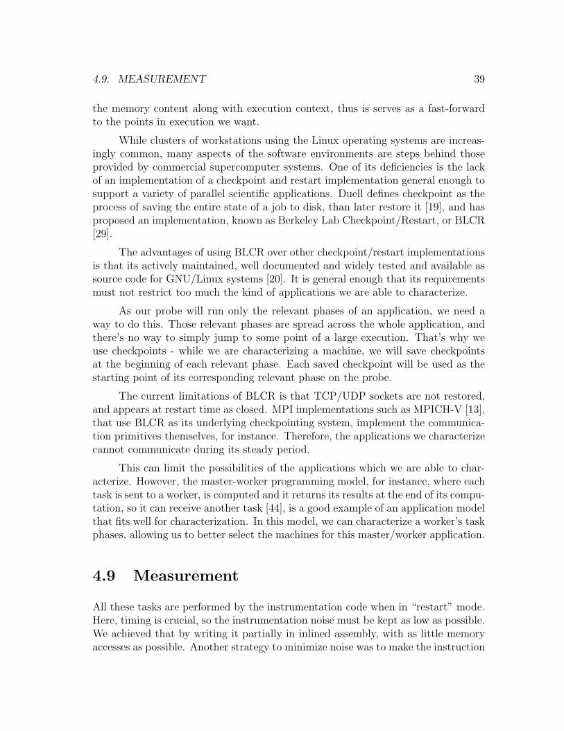
4.9. MEASUREMENT 39

the memory content along with execution context, thus is serves as a fast-forwardto the points in execution we want.

While clusters of workstations using the Linux operating systems are increas-ingly common, many aspects of the software environments are steps behind thoseprovided by commercial supercomputer systems. One of its deficiencies is the lackof an implementation of a checkpoint and restart implementation general enough tosupport a variety of parallel scientific applications. Duell defines checkpoint as theprocess of saving the entire state of a job to disk, than later restore it [19], and hasproposed an implementation, known as Berkeley Lab Checkpoint/Restart, or BLCR[29].

The advantages of using BLCR over other checkpoint/restart implementationsis that its actively maintained, well documented and widely tested and available assource code for GNU/Linux systems [20]. It is general enough that its requirementsmust not restrict too much the kind of applications we are able to characterize.

As our probe will run only the relevant phases of an application, we need away to do this. Those relevant phases are spread across the whole application, andthere’s no way to simply jump to some point of a large execution. That’s why weuse checkpoints - while we are characterizing a machine, we will save checkpointsat the beginning of each relevant phase. Each saved checkpoint will be used as thestarting point of its corresponding relevant phase on the probe.

The current limitations of BLCR is that TCP/UDP sockets are not restored,and appears at restart time as closed. MPI implementations such as MPICH-V [13],that use BLCR as its underlying checkpointing system, implement the communica-tion primitives themselves, for instance. Therefore, the applications we characterizecannot communicate during its steady period.

This can limit the possibilities of the applications which we are able to char-acterize. However, the master-worker programming model, for instance, where eachtask is sent to a worker, is computed and it returns its results at the end of its compu-tation, so it can receive another task [44], is a good example of an application modelthat fits well for characterization. In this model, we can characterize a worker’s taskphases, allowing us to better select the machines for this master/worker application.

4.9 Measurement

All these tasks are performed by the instrumentation code when in “restart” mode.Here, timing is crucial, so the instrumentation noise must be kept as low as possible.We achieved that by writing it partially in inlined assembly, with as little memoryaccesses as possible. Another strategy to minimize noise was to make the instruction

40 CHAPTER 4. PROBE

count updated only at the end of each basic block and inlined, instead of after eachinstruction. This made the code almost 50 times faster (thus less intrusive) thanbefore. The instrumentation noise is one inlined branch instruction (the JE) andone operator decrement (count–) per basic block, which is around 1% of it in ourexperiments.

When restoring execution from a checkpoint, a side effect will happen. Thecaches and predictors will not be in a consistent state with what would be done ina full execution that happened from the beginning up to that point. The process ofputting the machine in a state similar of that from a full execution is called warmup[30]. We use a warmup size of 7,000 instructions, as stated as enough by Laha [46].On that time, caches were much smaller than today’s multi-megabyte caches ofmodern processors, but still, we did not have any observable difference in predictionprecision when changing this value from 7,000 up to 50,000 instructions. In ourexperiments, we used a phase length interval of 100 million instructions, which wasnoted big enough to mitigate cache warmup effects.

After the number of instructions executed is the size of our interval (the in-strumentation itself is not counted), instrumentation sends a signal (the Unix’sSIGSTOP) to pause the application execution and measures the time, then it stopsthe application execution (With SIGKILL). The reason for using SIGSTOP firstis that it pauses immediately, without taking any further action, so it’s immedi-ate. After measuring the time, the instrumentation sends a SIGKILL, which freesmemory, sockets, handlers and so on, which takes a short, but perceptible and un-determined time. When the process is terminated, the shell script regains controland can proceed to restart/resume from the next phase.

In order to extrapolate the execution time, it is necessary to have a base valuefor comparison. So, with the execution time of the full application uninstrumentedwhen compared to the instrumented one in the reference machine, we are able tocalculate instrumentation noise (see Figure 4.4), which tends to be a fixed portionof execution time - i.e., it tends to keep the same amount of noise regardless of themachine we are running our Probes at, so we consider it constant. So on our referencemachine we calculate the noise as the proportion between the time it takes to run thewhole application on the reference machine with the phase instrumentation ETRefand the uninstrumented execution time ETuninstRef .

(4.3) Noise =ETRef

ETuninstRef

We calculate the proportion of each phase time and the total execution time,instrumented, on the reference machine. This is given by the formula in equation

4.9. MEASUREMENT 41

“Clean” execution - i.e. No instrumentation

(1)

“Noisy” (instrumented) execution

(2)

Figure 4.4: Instrumentation noise. The dark dots are instrumentation instructionsinserted in the execution during runtime.

4.4, where ETRef is the full execution time with instrumentation in the referencemachine, Weight is this phase’s weight, and TPhaseRef is the time this phase tookto run on the reference machine.

(4.4) TimeUnitV alue =(ETRef ∗ Weight)

TPhaseRef

For example, if the application takes 120 seconds to run, and one phase takes3 seconds, but this phase’s weight is 50% of the total execution, by substitution,each second of this phase is worth (120 · 0, 5)/3 = 20 seconds of the full executiontime.

With the time unit value, it is easy to extrapolate the execution time of thephase probed regarding to the full execution

(4.5) PhasePredicted = TimeUnitV alue ∗ TProbed

With all the data, we are able to predict our execution time as can be seen inequation 4.6

(4.6) ETPredicted =(∑numPhases

i=1 PhasePredicted)

Noise

42 CHAPTER 4. PROBE

(4.9) CPerfavail =∑

workers

PerfAvail

As Noise itself is a fraction, we multiply the predicted execution time by itsinverse. The final result is given by equation 4.7:

(4.7)

ETPredicted = (numPhases∑

i=1

(ETRef ∗ Weighti)

TPhaseRefi

∗ TiProbed) ∗ ETuninstRefETRef

4.10 How it fits in the multi-cluster model

In the multi-cluster performance model developed by [9], a methodology to improvethe execution time of master/worker applications in multi-clusters was developed.The performance model can predict the execution of the whole applications pro-vided it knows beforehand the network throughput and the time it will take forcompleting a task in each and every of the available computing elements. Thesteady performance model (that is, after initialization of all workers) is given byPerfSte in equation 4.8.

(4.8)

PerfSte = min

(CPerfAvail, Oper ∗

TPutEC

SComm

, Oper ∗ N ∗ TPutInetIN

STaskInter

, Oper ∗ N ∗ TPutInetOUT

SResultInter

)On this equation, CPerfAvail is given by equation 4.9, Oper is the number of

basic operations of a task, TPutEC is the external cluster LAN average throughput,SComm is the total communication of a task, N is the number of the tasks of this exe-cution, TPutInetIN is the external cluster’s internet incoming throughput, STaskInter

is the size of an inter-cluster task, TPutInetOUT is the the external cluster’s outgoingthroughput, and SResultInter is the inter-cluster’s task size.

Every parameter of this equation is either a factor of the network throughputs,which are straightforward to discover and problem size, which is known beforehand,and that sub-cluster available performance, described in equation 4.9.

On it, PerfAvail is the relative computation performance of a machine whilerunning a worker task. While every other parameter of these equations is discov-erable or already known, this one is not, neither is trivial to be discovered. In this

4.10. HOW IT FITS IN THE MULTI-CLUSTER MODEL 43

0Mb

2.000Mb

4.000Mb

sweep 3d 50 n.Body bt.B sweep3d 150

Probe sizes in megabytes

Figure 4.5: Probe sizes.

methodology, to determine the performance of the application, a whole long-runningtask was sent to every available node on the whole multi-cluster. That may takelong times, according to the time of a single worker task.

What our Probe does is to fill this gap of the PerfAvail value in Argollo’sresearch in a way fast enough that the model can determine the value for thisvariable to make dynamic adaptations to the performance of the multi-cluster. Thisway it is possible to reschedule tasks and discard those computing elements notfast enough to help with the computation efficiently during execution, with no needfor a previous setup stage for performance discovery, which greatly enhances theusefulness of his model.

44 CHAPTER 4. PROBE

Chapter 5

Reduced Probe

Off with her head!— The Queen

5.1 Introduction

Chapter 4 described the basic concept of the probe, how to build it and what it does.One issue with this methodology is that by generating a number of checkpoints inorder to characterize an application means that the Probes themselves can be prettylarge.

In previous experiments, we found Probes in order of gigabytes. In chapter 6,one of the Probes is around 1.3 gigabyte. This means a transmission time of aroundthree hours in a 1Mbps connection, something not totally unusual on the Internet.A strategy to reduce probe size was essential to make it useful in the multi-clusterenvironment.

In order to make the program mimic the functionality of the original applica-tion, two parameters are essential: memory access pattern and program flow.

5.1.1 Memory access pattern

Some researchers, as Toomula and Subhlok, for instance, go as far as to say thatreplicating only the memory access pattern is enough to predict performance [83], asaccess times for modern memories are orders of magnitude longer than computingtime, and a cache failure can account for hundreds of clock cycles spend with theCPU being idle.

Other researchers, such as Weinberg et. al. [90], try to match the temporal and

45

46 CHAPTER 5. REDUCED PROBE

spatial locality of memory access patterns of HPC applications with those of somebenchmarks. Their insight is that it is possible to derive application performance in amachine from metrics given by execution of such benchmarks and its correspondency.

Andrade et.al. even developed a method to guide the compiler optimizationprocess in respect to cache miss probability [4], [3], [6], [5].

Hollingsworth created a tool which is able to model memory patterns to predictthe performance of future computing systems [35]. So we can safely assert that thememory access pattern is one of the important factors for performance prediction.

5.1.2 Program control flow

The other parameter relevant for performance prediction is the program control flow.Modern processor cores have multiple pipelines and duplicated functional units forthread parallelism, among other characteristics. To fully mimic a program behavior,computation is important as well.

The control flow is closely associated to the memory access pattern, as thedecision flow is usually related to the contents of the memory in some moment.

Our initial research on mimicking only the memory access patterns to theexclusion of all other factors did not produce the performance prediction precisionrequired to feed the multi-cluster scheduler with any useful informatio, so this linewas promptly abandoned. One outcome of the need to keep the computation andthe call path and decision flow of the application to be characterized is that thememory contents must also be kept in the Probe. Which, as already stated, leads tosizes big enough to diminish the usefulness of the probe on our target environment,the Internet.

As our research advanced through the use of checkpoints, it became evidentthat the sizes of the Probes were getting bigger with every iteration of applications.Memory capacity is increasing steadily, so are the data sets of scientific applications.

However, our empirical observations suggests that the average internet speed isnot following suit. So these two factors: data sets already big (and therefore, Probes)getting even bigger, and the network not becoming faster on the same proportion,urged us to look to this issue of Probe size as a priority.

So we started to seek ways of reducing the Probe size, and this is furtherexplained in this chapter.

5.2. REDUCTION 47

5.2 Reduction

We investigated multiple ways to reduce Probe size. Currently, we use three differentmethods.

They are:

• Removal of less-important phases,

• Compression, and

• Touched set approach.

They will be detailed on the following sections.

5.3 Removal of less-important phases

This approach is straightforward - it consists of selectively not carrying the check-points of the less relevant phases. The tradeoff here lies between a possibly dramaticreduction of the Probe’s size, with little complexity, as it is just the removal of check-points of phases with lesser weights against the loss of precision.

With the weights in hand, we know exactly the remainder percentage of ourprediction stays. With a rule of three, we extrapolate that to the full execution.

This method is particularly useful in programs whose behavior is dominatedby a small number of functions. This seem to be the case in several scientificapplications, which perform transformations in data in very specific patterns.

Some example of extreme cases are those of workflow applications, where theindividual tasks that transform the data were already separated in the workflow’snodes. As current implementations of workflows’ nodes create separate executablefiles for each node, so we must create separate probes for each of them, and experi-ments shown us that these nodes are mostly dominated by one or two single phases,so it is difficult to remove any of those phases from the Probe.

In all our experiments, we set Simpoint to output a maximum of 30 phases.This is a number high enough to represent the whole application’s behavior in practi-cally every application we tested, even those with varying behavior during execution.The disadvantage is that it is also possible to come with a high number of phases,meaning big amount of checkpoints, up to a maximum of 30. We also tell Sim-point to automatically discard phases beforehand - those whose sum accounts for amaximum 1% of the overall execution are automatically discarded.


402MB

680MB

959MB

1.372MB

1.785MB

2.195MB

2.608MB

25%

50%

75%

100%

7 6 5 4 3 2 1

99,7% 99,6% 99,3% 98,8% 97,6%93,7%

51,9%

Number of remaining phases

Sweep3d.150

Probe size

Figure 5.1: Prediction Quality x Probe Size.

In these cases, the Simpoint algorithm can output a number of phases that arelittle to no relevant to the overall execution, such as initialization and end phases,and during changes from important parts of the overall execution. Several of thesephases can be discarded with little loss of prediction.

One example of phase removal is that of Figure 5.1. It shows the checkpointsizes (thus, the phases) of the SWEEP3D application and the overall predictionquality and how this quality degrades whenthe number of phases gets reduced. Itcan also be seen how the Probe’s size is also reduced.

This example shows that SWEEP3D’s execution is dominated by two distinctphases - and keeping only those two phases and discarding the remaining, less-important ones, still gives us a prediction accuracy of more than 93%.

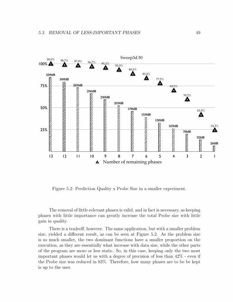
5.3. REMOVAL OF LESS-IMPORTANT PHASES 49

25%

50%

75%

100%

13 12 11 10 9 8 7 6 5 4 3 2 1

99,9% 98,7% 97,9% 96,7% 95,2% 93,0%88,5%

83,4%77,5%

69,5%

59,2%

41,8%

24,3%


Sweep3d.50

26MB

52MB

78MB

103MB

128MB

153MB

178MB

203MB

230MB

256MB

283MB

309MB329MB

Figure 5.2: Prediction Quality x Probe Size in a smaller experiment.

The removal of little-relevant phases is valid, and in fact is necessary, as keepingphases with little importance can greatly increase the total Probe size with littlegain in quality.

There is a tradeoff, however. The same application, but with a smaller problemsize, yielded a different result, as can be seen at Figure 5.2. As the problem sizeis so much smaller, the two dominant functions have a smaller proportion on theexecution, as they are essentially what increase with data size, while the other partsof the program are more or less static. So, in this case, keeping only the two mostimportant phases would let us with a degree of precision of less than 42% - even ifthe Probe size was reduced in 83%. Therefore, how many phases are to be be keptis up to the user.


5.4 Compression

Compression itself is a widely studied subject in computer science for decades andalien to the scope of this work, so it used only as a tool, as is. We use the gzipcompression tool, given its fast compression/decompression times, and its ubiquitouspresence in UNIX systems.

Compressing checkpoints as they were yielded different results according tothe workload and application, ranging from 20% to 35% of size reduction. So ithelps us achieve our goal of reducing the total Probe size, and it can - and is - usedaltogether with other approaches.

Slightly higher rates were obtained using other compression algorithms, asbzip2 and 7-zip, but the increase in compression/decompression times is dispropor-tional to the reductions in size. In essence, the time taken to compress a file using,say, bzip2, sending it to a remote cluster and decompressing it there is bigger thangzip in all our tests except with pathologically slow networks under 30kbps, theaverage speed of a dial-up connection in 1995. So we kept gzip for its simplicity,availability and speed.

5.5 Touched set approach

The touched set approach is based on two simple ideas:

• A Probe’s phase runs for a very limited amount of time, and is improbablethat in this time the program will access all its memory contents, and

• Every compression algorithm can benefit of large sequences of repeated char-acters, as all of them possess some form of run-length encoding [24].

A program’s phase basically consists in the application’s checkpoint in a spe-cific moment of time, that will have its execution time measured after a given numberof instructions is ran. In our experiments, this number is whether 10, 50 or 100 mil-lion instructions, but mostly 100 millions. In that interval - also known as trackingwindow [52], it is probable that only a subset of the application’s memory contentsits accessed. If a considerable amount of memory is not going to be used during aphase’s execution, this memory contents does not need to exist in the checkpoint.That is what we call touched set approach.

Touched set, as defined by Yawei and Zhiling [51] is the memory contentsaccessed during the interval - in our case, during a phase’s execution. All memorynot touched during the interval does not need to be present in the checkpoint.

5.5. TOUCHED SET APPROACH 51

X X X X X X X X (a)

(b)

0 0 0 0 0 0 0 0 0 0 0 0 0 0 0 0 0 0 0 0 0 0 0 0 (c)

8 * 0 1 2 * 0 (d)

Figure 5.3: Touched set approach

This means that the whole checkpoint is not necessary for running an interval,but instead, only the memory contents effectively accessed during this interval, asexemplified in Figure 5.3(a). On it, the memory accessed during the execution of agiven phase is marked with an “X”. As checkpoints have memory page granularitylevel, on Figure 5.3(b) we mark the pages to which these contents belong to asused, and on Figure 5.3(c), we fill the remaining contents with zeros, with can becompressed, as seen in Figure fig:touched-set(d). This means we can greatly trimthe checkpoints to carry as little information as possible, only the memory contentsthat are going to be required for reproducing the phase.

Our idea was that this approach could reduce the Probe sizes drastically.

We implemented the touched set approach in our probe system by intersectinginformation by modifying the code both for generating our Probes and that of thecheckpointing library kernel module, in the following way:

5.5.1 Probe generation

In the previous chapter, where we outlined the Probe generation process, the laststep was run the application to the end in our characterization machine, in order tosave the instrumented checkpoints.

The novelty we created to reduce the Probe size then is that now, in themoment right after saving a checkpoint, a trace of every memory page accessed


during its interval is recorded. That means, we still run the program thoroughlyand save the checkpoints, but during what would be the interval of this phase’sexecution, the address every single memory page accessed is recorded.

The reviewed algorithm of the probe becomes more or less like this:

The algorithm shown at figure 5.4 saves the checkpoint just at the beginningof the warmup period, as usual. However, the change comes when the warmupinterval has passed and the real phase point begins. On it, we dump the accessesto every memory page. Pin gives us instrumentation for memory accesses at bytelevel, but this precision is not necessary, and makes the trace files of memory accessesunreasonably large without any real need for it, as the checkpointing library mapsmemory pages and not individual bytes.

Which means that we either keep or remove one entire page at a time. If asingle byte in a page was touched, the whole page will be kept on the checkpoint.This reduces the possible compression gains, but it was necessary because not doingit made the instrumentation and the trace so heavy it did not fit the machines tested(some traces were estimated in the regions of dozens of terabytes for each phase).

So, in order to reduce trace file granularity, we perform the following binaryshift:

(5.1) memory page = memory access >> 12 << 12;

This effectively zeroes the twelve less-significant bits of the address, giving usa granularity of 4096 bytes, the standard page size of the Linux operating system.This greatly reduces the size of the trace, as an array transposition, for instance,would generate a single line for every 4096 positions, instead of one for each elementaccessed.

Besides this trace, additional information is required, which is discussed onthe next session:

5.5.2 Checkpointing library kernel module

The memory access trace must be matched with the contents on the checkpoints.The problem was that BLCR’s checkpoint file structure is not documented, and theheaders are of variable size.

In order to know the offset where a given memory page is recorded on this file,we had to modify the checkpoint kernel module to also create a trace of the tuple[memory page address / file offset].


phases=[simpoint output];


WARMUP=7000; // Instructions for warmup


counter=MAX_INSTRUCTIONS; // Negative counter of one phase

if(mode==MONITORING):

switch(inscounter):

case phases[x]*MAX_INSTRUCTIONS - WARMUP): // Point to checkpoint

make checkpoint;

x++;

break;

case phases[x]: // Point to start monitorin memory accesses:

// Instrument only the instructions that touch main memory

mem_address=instrument(instr_mem_access, memory_effective_address);

// Granularity is at byte level, but checkpoint works at

// memory pages level, so only stores page addresses.

mem_page=mem_address >> 12 << 12;

break;

default:

inscounter++;

else if(mode==RESTART_FROM_CHECKPOINT):

start_time=time.now();

loop: if(counter--==0): // JE in asm

stop_execution;

end_time=time.now();

printf(start_time, end_time);

exit(0);

Figure 5.4: Pseudocode for monitoring memory page addresses


With the touched set and the information given by the kernel module in hands,the only data required to stay in the checkpoint file is:

• File header,

• Process information required for restoring (pid, uid, gid, etc.),

• Part of the code segment (the one being used in this phase),

• The touched set.

The memory not accessed during the execution of the Phase interval is effec-tively discarded.

The touched set ξ in the checkpoint file is given by the set definition 5.2:

(5.2) ξ = (θ ∩ ϕ)

And the set of pages ζ to be removed from the checkpoint file is in definition5.3:

(5.3) ζ = (θ ∪ ϕ)− ξ

Where θ is the touched set as recorded when running the phase, and ϕ is theoffset of those pages in the checkpoint file. Everything else can then be removedfrom the checkpoint file, thus reducing its size drastically.

Our first approach was to simply trim ζ from the checkpoint file, and changethe headers accordingly, in order to denote where each memory page part of ξ is,directly reducing checkpoint’s file size, as the non-used portions were not recordedat all, making it a densely-populated file. This presented some major drawbacks:

• Implementation cost: the checkpointing library needed to be extensively changedin the restart code, in order to accommodate the “jumps” we created on thepages’ sequence, and

• Binary compatibility: as the checkpoint restart code was changed, we had acheckpointing library kernel module that needed to be installed in every systemwe would test our probe, which would break with the premise for the electionof BLCR as the checkpointing library of choice given its availability in severaldifferent clusters, and we would not be able to restore “regular” checkpointfiles on that, either, breaking functionality for other users.


For that reason, we created a simpler approach:

The memory pages present in the set ζ, that, for our purposes, can be discardedare instead filled with zeros, so the file can be now considered sparse.

The implementation of that is a Python program that reads all addressesof memory pages from the kernel module output for this specific checkpoint andtransforms it into a vector of tuples containing the memory page and file offset.Then, it reads the trace of memory pages accessed during the execution of thisinterval, and excludes the pages read from the trace file from its vector. The positionsthat remain on the vector are those which were not accessed during this phase, andare therefore zeroed out in the checkpoint file.

The biggest advantages are:

• It keeps binary compatibility with standard BLCR installations in other clus-ters - which was really welcome by these clusters’ administrators, our check-points are binary-compatible with the standard BLCR;

• Although the checkpoint file itself does not change, compression ratios increasegreatly, as the memory pages that were discarded now are just big sequencesof zeroes, which even the most primitive run-length encoding compressionalgorithm is able to take advantage of.

In resume, the steps are:

• The program is executed, instrumented;

• Simpoint runs over the BBV file and discovers the phases;

• The program is run again, instrumented, and makes checkpoints at the momentof a phase warmup with information about the memory pages’ offset in thefile dumped from the kernel module;

• The program keeps running. When it passes the warmup phase, it startsdumping the memory page addresses until the end of the phase;

• The program keeps running and doing the two previous points until all phasesare checkpointed and traced;

• With the memory trace and checkpoint offsets matched, the memory pages ζare zeroed from the checkpoint by a special utility;

• Previous point is made for all checkpoints;


• Probe can be compressed now, with the sparse checkpoint files, which reducesthem significantly.

So, after the program was characterized, its phases discovered, the phasessaved, a special program gathers the data coming from the kernel and that from thememory trace for each phase.

Then it creates the set ζ and zeroes it from that checkpoint’s phase and com-presses this now sparse file. Then it proceeds to the next phase, up to when thereare no more phases to reduce.

The final output is a set of gzipped files. One further idea to reduce probe sizeis one characteristic of gzip compression: it can be decompressed before the wholefile is present. So a probe could be sent through the network and uncompressed onthe fly, with a pipe from the process receiving the byte stream to the gunzip utility.This eliminates the need to receive the whole file and then start the uncompressionprocess, masking the time required for it, as it is done while receiving the file.

The resulting file on the other end is a checkpoint file containing only thememory contents required for running the original application’s phase from thewarmup to the phase’s size plus a very light instrumentation required to measurephase execution time. After the phase reaches its designated number of instructions,time is registered and the execution is interrupted, allowing the execution of the nextphase.

The combination of the aforementioned methods: removal of little-relevantphases, touched set approach and compression is what allows us to achieve greatreductions in probe size, up to 95% smaller when compared to the original set ofcheckpoints, as we will show in the next chapter.

Several characteristics that can be seen in our method are not from the methodper se, but instead it reflects those from the tools used to build this prototype. Someof them are:

• The application’s binary and its open files must be present in the same loca-tions on the machine to be characterized: This is a characteristic of BLCR,not of our method.

• Instrumentation library’s .so files must be present on the machine to be char-acterized, on the same location: same as again, a requirement from BLCR. AsBLCR does not “see” the instrumentation library, but instead thinks that itis part of the application itself, it requires them to be on the same location onthe file system.


• Sockets are not restored by default: special support from, for instance, MPIlibraries, must be present for restoring network connections. As we are char-acterizing the worker during its steady state, this is not really important atthis moment.


Chapter 6

Experimental study

Begin at the beginning and go on till you come to the end: then stop.— The King

6.1 Introduction

As we seen on the previous chapters, this work studies the problem of characterizingthe performance of a given application running on a machine in a fraction of thetime required to run this application thoroughly.

The goal is to create knowledge of this application performance, so Argollo’smethod can use it to decide if this machine is worthy or not for execution accordingto an efficient threshold.

To reach this objective, we adopted the concept of a software probe that willrun only representative parts of an application. Those parts will provide us withperformance knowledge similar to the one which would be possible running the sameapplication entirely on the given machine and we can then predict execution time.

To prove the concept of the Probe, we did some experiments, both regardingthe accuracy of the probe as well as the possible gains in reductions. We charac-terized the applications and created the Probes in our reference machine. Then weran these Probes on another machine or machines, predicted the execution time andcompared with the real execution time on this machine.

On them, phases’ times were compared, and weights were applied to each ofthose phases. The weights are given to us by Simpoint, and they mean the numberof executions of that phase over the number of executions of all phases, i.e. itdescribes how important a phase is. This comparison made possible to extrapolatethe execution time on the probed machine.

59

60 CHAPTER 6. EXPERIMENTAL STUDY

The first experiment was done with a double-nested loop matrix multiplica-tion. Being a program with a well known behavior, we could verify if the methodand our tool worked as expected. Being so simple and with a known memory accesspattern (stride), Simpoint correctly found only one phase representative of 99,9%of program’s behavior. and the Phase found was close to the middle of the execu-tion. This proved that the general system works and that we might proceed to testexecution time of more complex applications.

6.2 Experimental results

We realized a series experiments to verify the quality of our prediction.

We ran and characterized the worker in Master/Worker versions of the ASC’sSweep3d [33], a Matrix Multiplication, a n-Body problem, the NAS Benchmarks[11] BT and DC, class B. We show these specific experiments because these specificproblem sizes took roughly similar execution times, although providing very distinctphase behavior. These are average results for the execution of a single worker. Thisprobing would be done on each and every node available for execution in the parallelenvironment.

The testbed consisted of one Intel Pentium4 2.6ghz“Northwood” with 1 giga-byte of RAM as reference machine, and the Probes were sent to a cluster of sevenIntel Pentium4 “Prescott” 2.88ghz machines with 512 megabytes of RAM, and acluster of Intel Pentium4 “Cedar Mill” 3.0ghz machines with 1024 megabytes ofRAM, all in a switched Fast Ethernet network.

Although Pentium 4 indicates the same technology, they are different proces-sors, with different manufacturing methods and transistor sizes. It is worth notingthat the comparisons is not only among CPUs, but instead the whole computer - asmall amount of memory may affect an application’s performance as much (or more,in extreme cases) than the number of pipeline stages or cache sizes.

In this work’s experiments, each cluster was homogeneous, although they wereheterogeneous among themselves. It means that we would be able to further speedcharacterization time by running different phases in different machines in parallel.If the clusters were heterogeneous, we also would gain time, as the Probe wouldbe sent just once for the whole cluster, and each machine would be able to run itwithout having to download it again from our location.

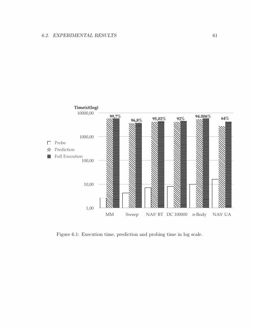
6.2. EXPERIMENTAL RESULTS 61

1,00

10,00

100,00

1000,00

10000,00

MM Sweep NAS’ BT DC 100000 n-Body NAS’ UA

ProbePredictionFull Execution

Time(s)(log)

99,7%96,8% 95,02% 92% 94.006% 64%

Figure 6.1: Execution time, prediction and probing time in log scale.


6.2.1 Precision

Figure 6.1 summarizes the prediction quality of our Probes. The bar in white is theexecution time taken by the Probe to run. The bars in light grey are the predictedexecution time calculated from these Probes’ executions, and the dark grey barsare real executions of the same applications on these machines. The graph is in logscale, because the Probes took orders of magnitude less time to run than the actualapplication and would not appear there at all otherwise.

We chose problem sizes who took similar execution times for the sake of pre-sentation. For the tested applications, the precision stood above 92%, while theprobing time was around 0.2% of the original application’s execution time for thisset of experiments, with the exception of NAS’ UA (more on that later). Longerapplications in general yields even better reductions, consequence of a higher num-ber of repetitions of the same phase. The probing time doesn’t take into accountcheckpoint transmission and checkpoint loading, instead focus on its phase executiontime.

The Matrix Multiplication is an obvious case, with a single phase that correctlyrepresented the execution time.

The Sweep3d application, using a grid of 150x150x150 units, possesses a mem-ory usage around 436 megabytes in most of its execution, except for the startup.Simpoint detects between 7 and 13 phases for it (according to the random dimensionprojection, the results can vary), with the behavior dominated in more than 90% bytwo phases, as shown in the previous chapter. In the case of ten phases, the Probeable to represent 99,7% of its total behavior actually predicted the execution timewith 96% accuracy with all phases. On the next section, we show the reductions insize and prediction for this experiment.

The NAS’ BT has three main phases that dominate more than 60% of theexecution time, but in total, it produced 17 different phases for the problem sizecategory B. The phases ran in less than ten seconds, but were able to predict theexecution time of the full execution, which took around two hours, with an error ofless than 5%.

The NAS’ DC had our worst prediction quality with the exception of UA. Thetime predicted from its Probe was 8% less than the real application. Yet, this is stillenough to show differences between execution times between different machines inorders of magnitude faster than the executions themselves.

The n-Body Probe was able to predict the execution time of the original ap-plication, with a correctness of 94%. Interestingly, this Probe had the smallest sizeof them all, keeping the state of the program around four megabytes throughoutthe whole execution. However, it was the probe that took longer to execute, close


to ten seconds for its ten phases. I suppose this has to do with a badly projectedapplication with a pathological number of cache misses. More studies on the imple-mentation and with other tools could give us some answers on this case. Still, theprediction information is enough for our purposes.

The UA case is special. It has a much worse prediction quality than anyother experiment. Turned out that the Simpoint found 16 phases for it, but ourreduced probes from phases 11 to 16 failed to execute, as the checkpoint segfaultsimmediately after restarting on such phases, so it was a forced reduction in qualitywhich accounts to 38% of the execution, so our method was able to measure onlyabout 62% of the program’s behavior.

Upon further investigation, we realized that it might be a bug in the Pin toolkititself or in our instrumentation code: specifically where we trace individual memoryaccesses. It seems that some bytes accessed were not recorded by the trace, whichthen reported them as not used, prone to further trimming.

We suspect that it can be some data type very close to the border of a memorypage, which means that only the parts pertaining to the page where this data beganwere recorded, but not the bytes on the next memory page. Further research isnecessary.

However, when we took into account that the 62% was the remaining behaviorand extrapolated from it, the prediction still was over 91%, which indicates that thecomputation behavior, time-wise, of these phases was not that different from theprevious ones.

If we considered only the first ten phases as being representative of the wholeprogram and proceeded to reduce it using the techniques explained in the previouschapter, we would end up with a prediction quality of 53,4%, which, when extrapo-lated to the full execution, led us to predict the execution time of the UA benchmarkon this machine with an accuracy of 89,5%. This reduced probe was 87% percentsmaller than the one comprised by the original ten checkpoints, being reduced fromaround 221 megabytes to 27 megabytes.

6.2.2 Probe Transmission Time

As different programs have distinct number of phases, the number of checkpointsis evidently different. For the sake of illustration, we ran the Sweep3d applicationwith a smaller problem size. The first group used a 50-unit cube, which took about40 seconds to run. Our characterization method found 19 distinct phases in thisexecution, and the Probe comprised the application and these 19 checkpoints. Thesum of checkpoints’ sizes was more than 372 megabytes. Consequently, a set of files


this big would take a little bit over an hour to transmit over a 1 mbps network link,in the case the transmission is perfect. Also this specific case, our Probe would notworth the effort, as this is just an example of a very short execution where it tooklonger to be produced and sent than the execution time of the application itself.The obvious conclusion is that the longer the application’s execution time, the moreuseful the Probes become.

However, when looking at the n-Body example, its state was kept constantaround 4.2 megabytes, and the whole Probe had approximately 43 megabytes. Thisprogram took more than two hours to run, but the Probe’s transmission time wouldbe of only 5 minutes in the same hypothetic 1mbps network link. The time in ourmulti-cluster, with a fast network, is negligible.

When Sweep 3d used the 150-unit cube, the total Probe size was around 2.8gigabytes, while BT.B was around 1.8 gigabytes. Sending both of them wouldbe overkill, so now we experiment with reduced probes while trying to maintainprediction quality with the techniques explained on the previous chapter.

6.2.3 Reducing Probe size

Are those checkpoints really necessary? We set our characterization to reflect 99%of the execution, because we noted that this extra one percent gave us nothing inprediction quality while increasing enormously the number of checkpoints. But canwe go even further? Can we discard phases on purpose, while maintaining qualityon our precision? How much would the prediction quality loose while reducing theProbes to their bare minimum?

To answer to this question, we selectively verified our prediction quality withless and less phases. Figure 6.2 shows some of those results, We now proceed todiscuss them individually.

Sweep3d.50

Figure 6.3 shows us a short execution, therefore there’s no dominant behavior. Thismeans that phases are, in general, equally important, and the curve is smooth.

Although this makes easier to choose the prediction precision, it makes biggerProbe size reductions more difficult. We experimented with keeping the five mostrelevant phases. Before extrapolation with a rule of three, this kept the predictionquality in about 78% of the execution. But in this experiment, the original Probehad more than 400 megabytes; Reducing it with keeping only the five most relevantphases, trimming the probes using the touched-set approach and compressing the


0%

2%

4%

5%

7%

Probe Size reductions - % of the original size

Sweep3d 50 Swee3d 150 BT UA t-coffee

Figure 6.2: Reduction


25%

50%

75%

100%

20 19 18 17 16 15 14 13 12 11 10 9 8 7 6 5 4 3 2 1

99,7% 97,7% 95,6% 93,6% 91,6% 89,5% 87,5% 85,5% 83,4%79,4%

75,3%71,2%

67,1%

61,0%

54,9%

48,8%

42,7%

34,6%

26,5%

16,3%


Sweep3d.50

Figure 6.3: Prediction quality (without extrapolation) of the Sweep3D applicationwith the cube sized as 50 units

resulting files let the probe with 19,2 megabytes. Still, this execution is so shortthat there is little point in making this process for this application/data size pair.

Sweep3d.150

Interestingly, we had two wildly different executions of the Sweep3d during our tests.In Figure 6.4, we see that Simpoint gave us seven phases, where execution is highlydominated by two of them, being others of little relevance. With this data in hand,we can selectively remove the less important phases while maintaining the desiredprediction quality.

We decided to keep only the three most relevant phases in this experiment. Itsquality should be around 97%, which held true by the experiments. However, evenafter trimmed down to one third of its original size by discarding the less-relevantphases, the Probe is still a behemoth of 959 megabytes. It would take about 2h20mto be transferred in a 1mbps network link. The communication time is almost as


402MB

680MB

959MB

1.372MB

1.785MB

2.195MB

2.608MB

25%

50%

75%

100%

7 6 5 4 3 2 1

99,7% 99,6% 99,3% 98,8% 97,6%93,7%

51,9%


Sweep3d.150

Probe size

Figure 6.4: Prediction quality (without extrapolation, touched-set or compression)of the Sweep3D application with the cube sized as 150 units, versus probe size


big as the execution itself.

After using the touched-set approach and standard gzip compression, theProbe had 151 megabytes, a reduction of 94% from its original size of 2608 megabytes.In the 1mbps network link, this would take circa 20 minutes to be transferred.

A different execution of the same test gave us a totally different result. InFigure 6.5, the same application when run under our characterization method yielded14 phases, with around 87% of its behavior in the first nine phases, with no dominantbehavior.

This is caused by the random dimension projection algorithm in Simpoint.As the number of Basic Block Vectors and of Basic Blocks itself is huge, Simpointprojects those dimensions in a matrix of 15 dimensions in order to be computa-tionally feasible. As the selection algorithm uses a random seed, behavior like thatcan appear. We noticed that several of those phases with a weight about 10% ofthe execution are in the same steady state of the execution, which means that theyare actually similar. Their measured execution times and the checkpoint sizes wassimilar as well.

In this experiment, we kept the six most significant phases, which by itselfwould give us a quality of 70% of prediction of the total execution time. Withextrapolation, this value was 93% of the actual execution time on the probed ma-chines, so the methodology worked, even in this case. From the 5440 megabytesof the original Probe, the reduced version ended up with 330 megabytes, which isabout 6% of its original size. In a slow network of 1mbps, it would take close to 40minutes to send this Probe, so perhaps, a more drastic reduction is required in thepresence of such a slow network, sacrificing prediction.

BT.B

The case shown in Figure 6.6 is a typical case of a benchmark, whose behavior isdominated by a small number of phases. In this case, 3. With these three phases,after extrapolating the behavior from 61% to the entirety of this execution, wearrived to a prediction quality of 91% of the original execution time, in average,with a reduction of 93% of the Probe size.

t-Coffee

T-Coffee is a multiple sequence alignment package, used to align Protein, DNAand RNA sequences and to combine sequence information with protein structuralinformation, profile information or RNA secondary structures [56]. As seen in figure


402MB680MB

959MB

1.372MB

1.785MB

2.195MB2.534MB

2.957MB

3.379MB

3.800MB4.173MB

4.595MB

5.017MB

5.440MB

25%

50%

75%

100%

14 13 12 11 10 9 8 7 6 5 4 3 2 1

99,8% 99,5% 98,6%95,6%

92,3%87,4%

82,2%76,2%

70,1%

60,3%

49,8%

39,1%

28,4%

14,3%


Sweep3d.150

Probe size

Figure 6.5: Prediction quality (without extrapolation, touched-set or compression)of the Sweep3D application with the cube sized as 150 units, versus probe size


25%

50%

75%

100%

16 15 14 13 12 11 10 9 8 7 6 5 4 3 2 1

97,0% 96,5% 94,8% 92,9% 91,0% 88,9% 86,6%84,0%

81,3%78,5%

75,7%72,6%

69,1%

61,2%

41,4%

21,0%


NAS’ BT

192MB383MB

574MB765MB

955MB1.144MB

1.332MB1.519MB

1.714MB1.909MB

2.102MB2.296MB

2.489MB2.681MB

2.867MB3.053MB

Figure 6.6: NAS’ Bt.B


143MB

300MB

458MB

634MB

857MB

25%

50%

75%

100%

5 4 3 2 1

99,3% 98,8% 97,6%93,7%

51,9%


T-coffee 50

Probe size

Figure 6.7: Prediction quality (without extrapolation, touched-set or compression)of the t-coffee application.

6.7, about 94% of its execution time is dominated by two phases. During thesetwo phases, the application was working over a really small segment of data, soour reduction techniques left us with a Probe of a mere 5,6 megabytes, able to betransferred in under a minute even under our 1mbps network. This is a reductionof 98% from the original Probe, that was of 857 megabytes.


Chapter 7

Conclusion and future work

What is the use of repeating all that stuff, if you don’t explain it as you go on? It’s by farthe most confusing thing I ever heard!— The Mock Turtle

7.1 Work contribution

This research started in order to complement previous research of [9] on the multi-cluster model, where one of the parameters of the equation for performance predic-tion in such model was left out as future work.

One of the ways to characterize the performance of a worker to finalize suchresearch is what we call the software Probe.

Our Probe methodology is able to fill this gap and find the PerfAvail param-eter necessary for equation 4.9 mentioned in chapter 4, which is itself one of theparameters of the whole model, depicted as equation 4.8 in the same chapter.

The Probe is able to predict the execution time of a worker in a matter ofseconds, instead of much longer times took by running the whole worker, and muchmore precisely than trying to correlate the application with benchmarks.

Initial research demonstrated that the checkpoints’ sizes made the Probes toobig to be transported over the internet in feasible time. Further research reducedthe Probes to a fraction of their original sizes, making them small enough to betransported to remote clusters in order to characterize their machines in viabletime.

One characteristic of the current Probe model is that the prediction dependson the original application’s input data. This is not exactly a defect, but a inherentcharacteristic of the application to be characterized. If the application is data-

73

74 CHAPTER 7. CONCLUSION AND FUTURE WORK

dependent, so will the Probe be.

There are two aspects of the data-dependency “issue” that should be observed:

• Even when a data-dependent application yields wildly different results fromone execution to another with different data sets of equivalent sizes, the Probesstill fulfill their objective of give performance information to the scheduler, inthe sense that the same Probe while run in different machines gives differentresults - so it is still an useful result for the matter of machine selection.

• Being the Probes as fast as they are, it is possible to construct a set of pre-defined probes with different input data that correlates to the spectrum ofpossible performances. There is ongoing research on characterizing these dif-ferent input data sets started by Fritzsche, Rexachs and Luque [22], and theunion of both lines of research stands as a promising future work (see nextsection).

7.2 Publications

This research has had as outcome the publication of the following Papers:

• Software Probes: Towards a Quick Method for Machine Characterization andApplication Performance Prediction [80], which received the awards of bestpaper and best presentation on the 7th International Symposium on Paralleland Distributed Computing (ISPDC) in 2008,

• Software Probes: A Method for Quickly Characterizing Applications’ Perfor-mance on Heterogeneous Environments [79], presented on the Workshop onDesign, Optimization and Management of Heterogeneous Networked Systemsof the 38th International Conference on Parallel Processing (ICPP) in 2009,

• Improving Probe Usability [78], presented on the Cloud Computing and Ser-vices Workshop of the 25th IEEE International Conference on Advanced In-formation Networking and Applications (AINA), in 2011.

7.3 Future Work

Probes are useful enough in a series of other models, not only in master/workerapplications in hierarchical multi-clusters. In fact, any scheduling logic that needsinformation about how a given computing element will perform while running an

7.3. FUTURE WORK 75

application can benefit from the use of Probes. Selection algorithms such as [2] and[12] can be simplified with the performance prediction given by our Probes.

Environments such as grids and clouds can use our Probes directly to replacethe “benchmark” parameter of the schedulers, as it is way more related to the realapplication.

Different application models, such as workflows [41] may also benefit fromProbes, as we may run Probes for every node of the workflow on every machineavailable, and run the workflow nodes where they run best.

Although the applicability of our methodology in such environments seemsobvious, experiments to prove the usefulness of the Probes on them are necessary.

As already stated on the previous section, the work of Fritzsche, Rexachs andLuque [22] correlates input data sets with their performance characteristics, andit is able to predict the execution time of applications where the input data maychange it radically, such as the parallel traveling salesman problem (TSP) [54], ofthe parallel clustering and classification of large number of documents [63]. It usesclustering techniques to correlate the position of the cities in a 2d map and the citywhere the travel starts with the time taken for the TSP to find the solution.

Fritzsche’s solution for the specific problem of the TSP can be generalizedto different kinds of applications. Their limitation was that to correlate differentinput data, the execution time for the thousands of experiments required was not afeasible task. Our proposal of fast Probes can make that research more general toencompass any kinds of applications, and their research can improve ours in the caseof data-dependent applications, using a collection of probes of the same applicationwith different characteristics.

76

Bibliography

[1] The top 500 supercomputers list - http://www.top500.org, June 2011.

[2] I Al-Furiah, S Aluru, S Goil, and S Ranka. Practical algorithms for selec-tion on coarse-grained parallel computers. IEEE Transactions on Parallel andDistributed Systems, Jan 1997.

[3] D Andrade, M Arenaz, B Fraguela, and J Tourino. Automated and accuratecache behavior analysis for codes with irregular access patterns. In Proceedingsof Workshop on Compilers for Parallel . . . , Jan 2006.

[4] D Andrade, B Fraguela, and R Doallo. Analytical modeling of codes with arbi-trary data-dependent conditional structures. Journal of Systems Architecture,Jan 2006.

[5] D Andrade, B Fraguela, and R Doallo. Precise automatable analytical modelingof the cache behavior of codes with indirections. portal.acm.org, Jan 2007.

[6] Manuel Diego Andrade. Automated and accurate cache behavior analysis forcodes with irregular access patterns. Concurrency and Computation: Practiceand Experience, 19(18):2407–2423, 2007.

[7] Murali Annavaram, Ryan Rakvic, Marzia Polito, Jean-Yves Bouguet,Richard A. Hankins, and Bob Davies. The fuzzy correlation between codeand performance predictability. pages 93–104, 2004.

[8] E Argollo, A Gaudiani, D Rexachs, and E Luque. Tuning application in amulti-cluster environment. Proceedings of the Euro-Par 2006, pages 78–98, Jan2006.

[9] Eduardo Argollo and Emilio Luque. Performance prediction and tuning in amulti-cluster environment. Ph.D. Dissertation, Oct 2006.

[10] D Bailey. Unfavorable strides in cache memory systems (rnr technical reportrnr-92-015). Scientific Programming, Jan 1995.

77

http://www.top500.org

[11] DH Bailey, E. Barszcz, JT Barton, DS Browning, RL Carter, L. Dagum, andet al. Fatoohi. The nas parallel benchmarks. International Journal of HighPerformance Computing Applications, 5(3):63–73, Jan 1991.

[12] J Barbosa, J Tavares, and A.J Padilha. Linear algebra algorithms in heteroge-neous cluster of personal computers. hcw, 00:147, 2000.

[13] A. Bouteiller, T. Herault, G. Krawezik, P. Lemarinier, and F. Cappello.MPICH-V project: A multiprotocol automatic fault-tolerant MPI. Interna-tional Journal of High Performance Computing Applications, 20(3):319, 2006.

[14] Doug Burger and Todd M Austin. The simplescalar tool set, version 2.0.SIGARCH Comput. Archit. News, 25(3):13–25, 1997.

[15] M Cierniak, M Zaki, and W Li. Compile-time scheduling algorithms for aheterogeneous network of workstations. The Computer Journal, 40(6):356–372,1997.

[16] H Curnow and B Wichmann. A synthetic benchmark. The Computer Journal,Jan 1976.

[17] A.S Dhodapkar and J.E Smith. Comparing program phase detection techniques.Microarchitecture, 2003. MICRO-36. Proceedings. 36th Annual IEEE/ACM In-ternational Symposium on, pages 217– 227, 2003.

[18] Jack Dongarra. The linpack benchmark: An explanation. In E. Houstis, T. Pa-patheodorou, and C. Polychronopoulos, editors, Supercomputing, volume 297of Lecture Notes in Computer Science, pages 456–474. Springer Berlin / Hei-delberg, 1988.

[19] J Duell. The design and implementation of berkeley labs linux check-point/restart. Tr, Lawrence Berkeley National Laboratory, 2000.

[20] J Duell, PH Hargrove, and ES Roman. Requirements for linux check-point/restart. 2002.

[21] B Fraguela, R Doallo, and E Zapata. Probabilistic miss equations: evaluatingmemory hierarchy performance. IEEE Transactions on Computers, Jan 2003.

[22] P. Fritzsche. Podemos Predecir en Algoritmos Paralelos no Deterministas?Ph.D. dissertation, 2007.

[23] C Glasner and J Volkert. Adaps-a three-phase adaptive prediction systemfor the run-time of jobs based on user behaviour. CISIS ’09. InternationalConference on Complex, Intelligent and Software Intensive Systems, 2009., Jan2010.

78

[24] S Golomb. Run-length encodings (corresp.). Information Theory, IEEE Trans-actions on, 12(3):399 – 401, 1966.

[25] J Goux, J Linderoth, and M Yoder. . . . Metacomputing and the master-workerparadigm. Preprint MCS/ANL-P792-0200 . . . , Jan 2000.

[26] G Griem, L Oliker, J Shalf, and K Yelick. Identifying performance bottleneckson modern microarchitectures using an adaptable probe. Parallel and Dis-tributed Processing Symposium, 2004. Proceedings. 18th International, 2004.

[27] G Hamerly, E Perelman, and B Calder. How to use simpoint to pick simula-tion points. ACM SIGMETRICS Performance Evaluation Review, 31(4):25–30,2004.

[28] Greg Hamerly, Erez Perelman, Jeremy Lau, and Brad Calder. Simpoint 3.0:Faster and more flexible program phase analysis. Journal of Instruction LevelParallelism, Sep 2005.

[29] P.H. Hargrove and J.C. Duell. Berkeley lab checkpoint/restart (blcr) for linuxclusters. Journal of Physics: Conference Series, 46(1):494–499, 2006.

[30] J.W Haskins and K Skadron. Memory reference reuse latency: Acceleratedwarmup for sampled microarchitecture simulation. Performance Analysis ofSystems and Software, 2003. ISPASS. 2003 IEEE International Symposiumon, pages 195– 203, 2003.

[31] Kim Hazelwood, Dan Connors, David Kaeli, and Vijay Janapa Reddi. Using pinfor compiler and computer architecture research and education. ACM Sigplan2007, PLDI Tutorial 2007, Jun 2007.

[32] A Hoisie, O Lubeck, and H Wasserman. Scalability analysis of multidimensionalwavefront algorithms on large-scale smp clusters. Frontiers of Massively ParallelComputation, Jan 1999.

[33] A Hoisie, O Lubeck, and H Wasserman. Performance and scalability analysisof teraflop-scale parallel architectures using multidimensional wavefront appli-cations. International Journal of High Performance Computing Applications,pages 330–346, Jan 2000.

[34] JK Hollingsworth, BP Miller, and J Cargille. Dynamic program instrumen-tation for scalable performance tools. Scalable High-Performance ComputingConference, 1994. Proceedings of the, pages 841–850, 1994.

79

[35] JK Hollingsworth, A Snavely, S Sbaraglia, and K Ekanadham. Emps: An en-vironment for memory performance studies. Parallel and Distributed Process-ing Symposium, 2005. Proceedings. 19th IEEE International, pages 223b–223b,2005.

[36] K Hoste and L Eeckhout. Microarchitecture-independent workload characteri-zation. IEEE Micro, Jan 2007.

[37] L John. Spec cpu2000: Measuring cpu performance in the new millennium.IEEE Computer, Jan 2000.

[38] A Joshi, L Eeckhout, and L John. The return of synthetic benchmarks. spec.org.

[39] A Joshi, L Eeckhout, L John, and C Isen. Automated microprocessor stressmarkgeneration. Proceedings of International Symposium on High Performance . . . ,Jan 2008.

[40] Ajay Joshi, Lieven Eeckhout, Robert Bell, Jr, and Lizy John. Distilling theessence of proprietary workloads into miniature benchmarks. Transactions onArchitecture and Code Optimization (TACO, 5(2), Aug 2008.

[41] DS Katz, JC Jacob, E. Deelman, C. Kesselman, G. Singh, M.H. Su, GB Ber-riman, J. Good, AC Laity, and TA Prince. A comparison of two methods forbuilding astronomical image mosaics on a grid. In Parallel Processing, 2005.ICPP 2005 Workshops. International Conference Workshops on, pages 85–94,2005.

[42] Junghwan Kim, Jungkyu Rho, Jeong-Ook Lee, and Myeong-Cheol Ko. Cpoc:Effective static task scheduling for grid computing. High Performance Com-puting and Communcations, pages 477–486, 2005: Springer.

[43] W Korn and P Teller. . . . Just how accurate are performance counters? Per-formance, Jan 2001.

[44] V Kumar, A Grama, and A Gupta. Introduction to parallel computing: designand analysis of algorithms. cs.umn.edu, Jan 1994.

[45] Lizy Kurian and Lieven Eeckhout. Performance evaluation and benchmarking.Jul 2007.

[46] S Laha, JH Patel, and RK Iyer. Accurate low-cost methods for perfor-mance evaluation of cachememory systems. Computers, IEEE Transactionson, 37(11):1325–1336, 1988.

80

[47] J Lau, E Perelman, G Hamerly, T Sherwood, and B Calder. Motivation forvariable length intervals and hierarchical phase behavior. IEEE InternationalSymposium on Performance Analysis of Systems and Software, 2005.

[48] J Lau, J Sampson, E Perelman, G Hamerly, and B Calder. The strong cor-relation between code signatures and performance. Performance Analysis ofSystems and Software, 2005. ISPASS 2005. International Symposium on Per-formance Analysis of Systems and Software, pages 236–247, 2005.

[49] J Lau, S Schoemackers, and B Calder. Structures for phase classification. Per-formance Analysis of Systems and Software, 2004 IEEE International Sympo-sium on - ISPASS, pages 57– 67, 2004.

[50] C Lee, C DeMatteis, and J Stepanek. . . . Cluster performance and the implica-tions for distributed, heterogeneous grid performance. hcw, Jan 2000.

[51] Y Li and Z Lan. Frem: A fast restart mechanism for general checkpoint/restart.Computers, IEEE Transactions on, PP(99):1 – 1, 2010.

[52] Yawei Li and Zhiling Lan;. A fast restart mechanism for checkpoint/recoveryprotocols in networked environments. Dependable Systems and Networks WithFTCS and DCC, 2008. DSN 2008. IEEE International Conference on, pages217 – 226, 2008.

[53] J McCalpin and CA Oakland. An industry perspective on performance charac-terization: Applications vs benchmarks. Proceedings of the Third Annual IEEEWorkshop Workload Characterization, keynote address, Sept, 2000.

[54] J Mohan. Experience with two parallel programs solving the traveling salesmanproblem. osti.gov, Jan 1983.

[55] R Murphy and P Kogge. On the memory access patterns of supercomputer ap-plications: Benchmark selection and its implications. Computers, IEEE Trans-actions on, 56(7):937 – 945, Jul 2007.

[56] C Notredame, D G Higgins, and J Heringa. T-coffee: A novel method for fastand accurate multiple sequence alignment. J Mol Biol, 302(1):205–17, Sep 2000.

[57] L Pastor and J.L Bosquwe Orero. An efficiency and scalability model for het-erogeneous clusters is -. Cluster Computing, 2001. Proceedings. 2001 IEEEInternational Conference on AB -, pages 427–434, 2001.

[58] H Patil, R Cohn, M Charney, R Kapoor, A Sun, and A Karunanidhi. Pin-pointing representative portions of large intel itanium programs with dynamicinstrumentation. MICRO-37 2004. 37th International Symposium on Microar-chitecture, pages 81– 92, 2004.

81

[59] E Perelman, G Hamerly, and B Calder. Picking statistically valid and earlysimulation points. Parallel Architectures and Compilation Techniques, 2003.PACT 2003. Proceedings. 12th International Conference on, pages 244– 255,2003.

[60] A Petitet, R Whaley, J Dongarra, and A Cleary. A portable implementationof the high-performance linpack benchmark for distributed-memory computers.Innovative Computing Laboratory, Jan 2004.

[61] A Phansalkar and L John. Performance prediction using program similarity.Proceedings of the 2006 SPEC Benchmark Workshop, Jan 2006.

[62] George A. Reis, Jonathan Chang, David I. August, Robin Cohn, and Shub-hendu S. Mukherjee. Configurable transient fault detection via dynamic binarytranslation. In IN: PROCEEDINGS OF THE 2ND WORKSHOP ON ARCHI-TECTURAL RELIABILITY. Citeseer, 2006.

[63] A Ruocco and O Frieder. Clustering and classification of large document basesin a parallel environment. Journal of the American Society for InformationScience, Jan 1997.

[64] I Sharapov, R Kroeger, G Delamarter, and R Cheveresan. A case study in top-down performance estimation for a large-scale parallel application. . . . ACMSIGPLAN symposium on Principles and practice of parallel . . . , Jan 2006.

[65] T Sherwood, E Perelman, and B Calder. Basic block distribution analysisto find periodic behavior and simulation points in applications. InternationalConference on Parallel Architectures and Compilation Techniques, Jan 2001.

[66] T Sherwood, S Sair, and B Calder. Phase tracking and prediction. Proceedingsof the 30th Annual International Symposium on Computer Architecture, 2003,pages 336 – 347, 2003.

[67] Timothy Sherwood, Erez Perelman, Greg Hamerly, and Brad Calder. Auto-matically characterizing large scale program behavior. SIGPLAN: Proceedingsof the 10th international conference on Architectural support for programminglanguages and operating systems, 37(10):45–57, 2002.

[68] Timothy Sherwood, Erez Perelman, Greg Hamerly, Suleyman Sair, and BradCalder. Discovering and exploiting program phases. IEEE Micro, Jan 2004.

[69] H Siege, L Wang, J So, and M Maheswaran. Data parallel algorithms.docs.lib.purdue.edu.

82

[70] A Snavely, L Carrington, N Wolter, and J Labarta. A framework for perfor-mance modeling and prediction. Supercomputing, Jan 2002.

[71] A Snavely, X Gao, C Lee, N Wolter, J Labarta, J Gimenez, and P Jones.Performance modeling of hpc applications. Parallel Computing (ParCo2003),2003.

[72] S Sodhi and J Subhlok. Skeleton based performance prediction on shared net-works. Cluster Computing and the Grid, 2004. CCGrid 2004. IEEE Interna-tional Symposium on, pages 723–730, 2004.

[73] S Sodhi and J Subhlok. Automatic construction and evaluation of performanceskeletons. Proceedings of the 19th IEEE International Parallel and DistributedProcessing Symposium (IPDPS’05), pages 88–98, Apr 2005.

[74] S Sodhi, J Subhlok, and Q Xu. Performance prediction with skeletons. ClusterComputing, Jan 2008.

[75] E Strohmaier and H Shan. Architecture independent performance character-ization and benchmarking for scientific applications. Modeling, Analysis, andSimulation of Computer and Telecommunications Systems, 2004.(MASCOTS2004). Proceedings. The IEEE Computer Society’s 12th Annual InternationalSymposium on, pages 467–474, 2004.

[76] E Strohmaier and H Shan. Apex-map: A synthetic scalable benchmark probeto explore data access performance on highly parallel systems. LECTURENOTES IN COMPUTER SCIENCE, 3648:114, 2005.

[77] E Strohmaier and H Shan. Apex-map: a parameterized scalable memory ac-cess probe for high-performance computing systems: . . . . Concurrency andComputation: Practice & Experience, Jan 2007.

[78] Alexandre Strube, Emilio Luque, and Dolores Rexachs. Improving probe us-ability. Cloud Computing and Services Workshop, The 25th IEEE InternationalConference on Advanced Information Networking and Applications (to appear),2011.

[79] Alexandre Otto Strube, Dolores Rexachs, and Emilio Luque. Software probes:A method for quickly characterizing applications’ performance on heteroge-neous environments. Parallel Processing Workshops, International Conferenceon, 0:262–269, 2009.

83

[80] AO Strube, Dolores Rexachs, and Emilio Luque. Software probes: Towards aquick method for machine characterization and application performance pre-diction. Parallel and Distributed Computing, 2008. ISPDC ’08. InternationalSymposium on Parallel and Distributed Computing, pages 23–30, 2008.

[81] J Subhlok, P Lieu, and B Lowekamp. Automatic node selection for high per-formance applications on networks. Proceedings of the seventh ACM SIGPLANsymposium on Principles and practice of parallel programming, pages 163–172,1999.

[82] H Sutter. The free lunch is over: A fundamental turn toward concurrency insoftware. Dr. DobbOs Journal, 30(3):202–210, 2005.

[83] A Toomula and J Subhlok. Replicating memory behavior for performance pre-diction. Proceedings of the 7th workshop on Workshop on languages, compilers,and run-time support for scalable systems, pages 1–8, 2004.

[84] Haluk Topcuouglu, Salim Hariri, and Min-you Wu. Performance-effective andlow-complexity task scheduling for heterogeneous computing. IEEE Transac-tions on Parallel and Distributed Systems, 13(3):260–274, 2002.

[85] Helmut Wanek, Erich Schikuta, and Irfan Ul Haq. Grid workflow optimizationregarding dynamically changing resources and conditions. In GCC ’07: Proceed-ings of the Sixth International Conference on Grid and Cooperative Computing,pages 757–763, Washington, DC, USA, 2007. IEEE Computer Society.

[86] V Weaver and S McKee. Can hardware performance counters be trusted?Workload Characterization, Jan 2008.

[87] V.M. Weaver and S.A. McKee. Using dynamic binary instrumentation to gen-erate multi-platform simpoints: Methodology and accuracy. Proceedings of the3rd international conference on High performance embedded architectures andcompilers, 4917:305–309, 2008.

[88] VM Weaver and SA McKee. Using dynamic binary instrumentation to gener-ate multi-platform simpoints: Methodology and accuracy. Proceedings of the3rd international conference on High performance embedded architectures andcompilers, 4917:305–319, 2008.

[89] R Weicker. Dhrystone: a synthetic systems programming benchmark. Com-munications of the ACM.

[90] J Weinberg. Quantifying locality in the memory access patterns of hpc appli-cations. 2005.

84

[91] A. Wong, D. Rexachs, and E. Luque. Parallel application signature. In ClusterComputing and Workshops, 2009. CLUSTER ’09. IEEE International Confer-ence on, pages 1 –10, aug. 2009.

85

Documents

Live long and Prosper! - UAB Barcelona · 2015. 2. 28. · the lovely Aram . Thanks, thanks a lot. Thanks also Gustavo and Alexandra, my great friends, thanks for your patience with