Embed Size (px)
Citation preview

LISO - Program for Linear Simulation and Optimization
of analog electronic circuits – Version 1.7
G. Heinzel, NAO Mitaka
November 9, 1999
New features of version 1.7
For the benefit of those users who have been using LISO version 1.33, here is a shortlist of the most important new features:
• The circuit can contain transmission lines as additional passive circuit elements(see Section 6.5 on page 18).
• The noise can also be computed as current through one component, not onlyvoltage at one node (see Section 7.3 on page 28).
• The noise at the output can be referred to the input, i.e. divided by the transferfunction (see Section 7.3.2 on page 29).
• The sensitivity of any of the computed results (such as transfer function, noiseetc.) to small variations in the components can be computed and printed intabular form (see Section ?? on page ??).
• The dynamical range of a circuit can be optimized with additional fitting con-straints (see Section 10.5 on page 41).
• New fitting algorithms offer improved convergence for poor starting values (seeSection 4.1 on page 9).
• Various improvements in the fitting part offer intermediate results and improveddiagnostics.
• In the uinput and iinput instructions, the specification of the source-impedanceis optional (see Section 6.7 on page 21).
• A voltage input (uinput instruction) can be floating. (see Section 6.7 on page 21).
Contents
1 Introduction 5
1

2 Availability 5
3 Features and limitations 6
4 Invoking LISO 8
4.1 Options . . . . . . . . . . . . . . . . . . . . . . . . . . . . . . . . . . . . 9
5 The input file 10
5.1 General remarks . . . . . . . . . . . . . . . . . . . . . . . . . . . . . . . 10
5.2 Instruction summary . . . . . . . . . . . . . . . . . . . . . . . . . . . . . 11
5.3 Example . . . . . . . . . . . . . . . . . . . . . . . . . . . . . . . . . . . . 14
6 Circuit description 15
6.1 Overview . . . . . . . . . . . . . . . . . . . . . . . . . . . . . . . . . . . 15
6.2 Nodes . . . . . . . . . . . . . . . . . . . . . . . . . . . . . . . . . . . . . 16
6.3 Simple passive components . . . . . . . . . . . . . . . . . . . . . . . . . 17
6.4 Mutual inductances . . . . . . . . . . . . . . . . . . . . . . . . . . . . . 17
6.5 Transmission lines . . . . . . . . . . . . . . . . . . . . . . . . . . . . . . 18
6.6 Op-amps . . . . . . . . . . . . . . . . . . . . . . . . . . . . . . . . . . . . 21
6.7 Input definition . . . . . . . . . . . . . . . . . . . . . . . . . . . . . . . . 21
6.8 Input factor . . . . . . . . . . . . . . . . . . . . . . . . . . . . . . . . . . 22
7 Circuit mode: requesting output 23
7.1 Transfer functions . . . . . . . . . . . . . . . . . . . . . . . . . . . . . . 23
7.1.1 Treatment of the input . . . . . . . . . . . . . . . . . . . . . . . . 23
7.1.2 Specifying the output format . . . . . . . . . . . . . . . . . . . . 23
7.1.3 Voltage transfer functions . . . . . . . . . . . . . . . . . . . . . . 24
7.1.4 Current transfer functions . . . . . . . . . . . . . . . . . . . . . . 25
7.1.5 Maximum permissible input signal . . . . . . . . . . . . . . . . . 25
7.1.6 Input impedance . . . . . . . . . . . . . . . . . . . . . . . . . . . 26
7.1.7 Op-amp differential input voltages . . . . . . . . . . . . . . . . . 26
7.2 Op-amp stability . . . . . . . . . . . . . . . . . . . . . . . . . . . . . . . 27
7.3 Noise calculations . . . . . . . . . . . . . . . . . . . . . . . . . . . . . . . 28
7.3.1 Specifying the noise sources to be added . . . . . . . . . . . . . . 29
7.3.2 Input-referred noise . . . . . . . . . . . . . . . . . . . . . . . . . 29
2

8 Root mode 30
8.1 Transfer function definition . . . . . . . . . . . . . . . . . . . . . . . . . 31
8.1.1 Poles and zeroes . . . . . . . . . . . . . . . . . . . . . . . . . . . 31
8.1.2 Overall factor . . . . . . . . . . . . . . . . . . . . . . . . . . . . . 32
8.1.3 Frequency scaling . . . . . . . . . . . . . . . . . . . . . . . . . . . 32
8.1.4 Delay time . . . . . . . . . . . . . . . . . . . . . . . . . . . . . . 32
8.2 Requesting output of the transfer function . . . . . . . . . . . . . . . . . 32
8.3 Transfer function examples . . . . . . . . . . . . . . . . . . . . . . . . . 33
8.3.1 Lowpass . . . . . . . . . . . . . . . . . . . . . . . . . . . . . . . . 33
8.3.2 Highpass . . . . . . . . . . . . . . . . . . . . . . . . . . . . . . . 33
8.3.3 Bandpass . . . . . . . . . . . . . . . . . . . . . . . . . . . . . . . 34
8.3.4 Bandstop . . . . . . . . . . . . . . . . . . . . . . . . . . . . . . . 34
9 Sensitivity analysis 35
10 Fitting 35
10.1 Introduction . . . . . . . . . . . . . . . . . . . . . . . . . . . . . . . . . . 35
10.2 Function to be fitted . . . . . . . . . . . . . . . . . . . . . . . . . . . . . 36
10.3 Data file . . . . . . . . . . . . . . . . . . . . . . . . . . . . . . . . . . . . 36
10.3.1 Weighting . . . . . . . . . . . . . . . . . . . . . . . . . . . . . . . 37
10.4 Parameters . . . . . . . . . . . . . . . . . . . . . . . . . . . . . . . . . . 39
10.4.1 Dependent parameters . . . . . . . . . . . . . . . . . . . . . . . . 40
10.5 Additional fitting constraints for optimizing the dynamic range . . . . . 41
10.5.1 Input range constraint . . . . . . . . . . . . . . . . . . . . . . . . 41
10.5.2 Noise minimization . . . . . . . . . . . . . . . . . . . . . . . . . . 42
10.6 Rewriting the input file with best-fit parameters . . . . . . . . . . . . . 43
10.7 Output of the fitting procedure . . . . . . . . . . . . . . . . . . . . . . . 43
10.8 Hints for fitting . . . . . . . . . . . . . . . . . . . . . . . . . . . . . . . . 45
11 Plot options 48
11.1 Defining the frequency range . . . . . . . . . . . . . . . . . . . . . . . . 49
11.2 GNUPLOT terminals . . . . . . . . . . . . . . . . . . . . . . . . . . . . 49
12 Initialization file “fil.ini” 50
3

13 Op-amp library 51
13.1 Open-loop voltage gain . . . . . . . . . . . . . . . . . . . . . . . . . . . . 52
13.2 Op-amp noise . . . . . . . . . . . . . . . . . . . . . . . . . . . . . . . . . 53
13.3 Op-amp limits . . . . . . . . . . . . . . . . . . . . . . . . . . . . . . . . 54
14 Circuit simulation algorithm 55
14.1 Transfer functions . . . . . . . . . . . . . . . . . . . . . . . . . . . . . . 55
14.1.1 Transmission lines . . . . . . . . . . . . . . . . . . . . . . . . . . 57
14.2 Noise calculations . . . . . . . . . . . . . . . . . . . . . . . . . . . . . . . 58
14.2.1 Treatment of the input . . . . . . . . . . . . . . . . . . . . . . . . 59
14.2.2 Resistor noise . . . . . . . . . . . . . . . . . . . . . . . . . . . . . 59
14.2.3 Op-amp voltage noise . . . . . . . . . . . . . . . . . . . . . . . . 59
14.2.4 Op-amp current noise . . . . . . . . . . . . . . . . . . . . . . . . 60
14.3 Op-amp stability calculations . . . . . . . . . . . . . . . . . . . . . . . . 61
15 Fitting algorithms 61
15.1 Extensions to the Nelder-Mead Simplex algorithm . . . . . . . . . . . . 62
15.1.1 Computation of n+ 1 directions equally distributed in Rn . . . . 62
15.1.2 Derivation . . . . . . . . . . . . . . . . . . . . . . . . . . . . . . . 63
15.1.3 Example . . . . . . . . . . . . . . . . . . . . . . . . . . . . . . . . 63
15.1.4 Initialization and termination . . . . . . . . . . . . . . . . . . . . 63
15.2 Extensions to the Levenberg-Marquardt algorithm . . . . . . . . . . . . 64
15.2.1 Numerical derivatives . . . . . . . . . . . . . . . . . . . . . . . . 64
15.2.2 Application to complex data . . . . . . . . . . . . . . . . . . . . 64
15.2.3 λ search . . . . . . . . . . . . . . . . . . . . . . . . . . . . . . . . 66
15.3 Overall minimization strategy . . . . . . . . . . . . . . . . . . . . . . . . 66
15.4 Implementation of parameter limits . . . . . . . . . . . . . . . . . . . . . 67
15.5 Correlation matrix and confidence limits . . . . . . . . . . . . . . . . . . 68
16 Implementation notes 69
16.1 Internal scaling . . . . . . . . . . . . . . . . . . . . . . . . . . . . . . . . 69
16.2 Sparse matrices . . . . . . . . . . . . . . . . . . . . . . . . . . . . . . . . 70
16.3 Efficient noise computation using the transposed matrix . . . . . . . . . 70
17 Application examples 71
17.1 Root mode simulation . . . . . . . . . . . . . . . . . . . . . . . . . . . . 71
17.2 Root mode fit . . . . . . . . . . . . . . . . . . . . . . . . . . . . . . . . . 72
4

1 Introduction
The computer simulation of electronic circuits is a well-established discipline. Thewidely known program SPICE, e.g., is very powerful at simulating things such as MOStransistors, transient behaviour, integrated circuits, digital logic devices, etc. For manyof the circuits that we1 need, however, the emphasis is on other aspects:
• The frequency response of preamplifiers and active filters built with op-amps inthe presence of non-ideal op-amp characteristics (finite gain and strange phaseshifts around the unity gain frequency).
• The noise behaviour of such circuits.
• The stability of each op-amp in a complex circuit.
• The sensitivity of the circuit’s characteristics to small variations in the compo-nents.
• The desire to optimize some components of such circuits for a given purpose, suchas maximum dynamic range.
The frequency response of several interesting circuits had been found analytically bythe author using Mathematica, assuming ideal op-amps. The attempt to extendthese analytical models to real op-amps showed, however, that the analytical solutionsvery quickly become too complex to be useful. In particular the noise behaviour getsvery complicated to compute. SPICE models provided by op-amp manufacturers dousually not correctly predict the noise behaviour of the circuits. Therefore a programwas written that computes these aspects of a given circuit numerically.
Using the simulation as base, the additional fitting function is a powerful tool toanalyze, design and optimize circuits.
2 Availability
The program and this manual were written by Gerhard Heinzel, mainly during hisstay at the Max-Planck-Institut fur Quantenoptik in Garching, Germany. The presentaddress is:
Gerhard HeinzelSpace-Time Astronomy Section,National Astronomical Observatory,2-21-1 Ohsawa, Mitaka, Tokyo 181-8588, Japane-mail: gerhard.heinzelnao.ac.jp
The program was written for use by members of GEO600, TAMA and cooperatingprojects. Both program and manual are
1By “we” I mean mainly those people who design analog electronics for gravitational wave detec-tors. However, LISO may also be useful to design electronic circuits for other purposes and also foreducational purposes.
5

Copyright c© G. Heinzel 1997, 1998, 1999.
Various portions of software from other authors were used. These have copyrightsof their own, which allow free non–commercial use under certain conditions, such ascomplete unmodified distribution with all sources. Since at present this is not yet thecase, I ask everyone:
• Feel free to use LISO for any noncommercial application.
• Of course you may also give it to interested colleagues and friends.
• Please to not distribute LISO to the general public, such as by placing it on yourown website.
• For any wider distribution or non-scientific application, please contact the authorfirst.
• The author is interested to learn about the applications, usefulness, problems,wishes, bugs etc. of LISO.
• Of course no guarantee of any kind is given or implied, such as for the correctnessof any algorithm, model or result. Any application of LISO is at the full risk ofthe user.
LISO is available by ftp from:ftp.rzg.mpg.de in the directory/pub/grav/ghh/liso.
3 Features and limitations
The input to LISO is a fixed circuit consisting of passive components (any combinationof R, C, L, transformers and transmission lines) and op-amps. It can have a voltageinput (grounded or floating) or a current input (such as for photodiode preamplifiers).The program may compute and plot:
• The frequency response from the input to any component or node (in particular,the voltage at the output or the current through any component).
• The maximum permissible input signal, taking into account op-amp output volt-age, output current and slew rate.
• The stability of each op-amp in the circuit. Since op-amps are the only elementswith gain, this is equivalent to computing the stability of each closed loop in thecircuit and the stability of the circuit as a whole.
• The voltage noise at any node of the circuit (in particular the output), takinginto account Johnson noise of resistors and voltage noise and current noise ofop-amps. It can separate the individual contributions of these noise sources andidentify the dominating noise source for any frequency range.
6

• The spectral density of the noise current in each component, taking into accountthe same noise sources as in the above item.
• The sensitivity of any of the above results to small variations in the components.
Some features of the program include:
• The program uses a user-expandable library of op-amp models with their maincharacteristics. For each op-amp in the circuit, the library parameters can be“overridden” by individual parameters.
• A very important function of the program is its ability to fit the model to givendata (either measured data or ideal desired data) by varying specified componentsor parameters.
• All computations can be done with complex numbers. In particular, data mea-sured with phase can be properly fitted.
• Some effort has been made to incorporate state-of-the-art algorithms for the sim-ulation and fitting parts, i.e. the author believes that the results are accurate forreasonable inputs and they are delivered fast.
• In a separate mode of operation of the program, frequency responses can becomputed using the poles and zeroes of the transfer function as input instead ofa circuit description.
• Extensions to the basic fitting algorithm allow the user to find circuits with auser-specified transfer function under additional constraints such as a minimalallowed output swing and minimum noise.
• Two new fitting procedures Direct Search Simulated Annealing and ControlledRandom Search often converge to solutions even when no reasonable startingvalue are given.
• The combination of the last two items allows the user to almost automaticallyfind circuits with a specified transfer function and the maximum possible dynamicrange. Many of these solutions are almost impossible to find by other means.
• The results are plotted via GNUPLOT, which supports many different output‘devices’ (including Postscript) and allows the user to change the appearance ofthe plot in an easy and flexible way.
The program has at present several limitations. Some of them (marked with an aster-isk *) could possibly be overcome if necessary, others not.
• The circuit topology is fixed and must be known and entered by the user.
• All computations are done linearly in the frequency domain. In particular, theDC operating point is not computed. No time-domain analyses are performed.No non-linear components such as discrete semiconductors can be simulated.
7

• Only voltage-feedback op-amps can be simulated. *
• There is no graphical user interface. Input and output are done via ASCII files ina batch-mode like operation. Plots are produced by calling GNUPLOT. WithoutGNUPLOT, the only output is an ASCII data file, which may be plotted by othersoftware.
• At present the program has mainly been tested under various versions of UNIX(mainly LINUX, also SUN and IBM) and MS-DOS. There should, however, beno big problem in porting it to any reasonable operating system. It is entirelywritten in C and the preferred compiler is the GNU C-compiler.
• There is only a very simple electrical rule check (ERC) which will not detect manykinds of errors in the circuit (e.g. outputs connected to GND etc.) *
• Not all useful transfer functions can be entered by the present pole/zero syntax.*
4 Invoking LISO
LISO is started from the command line with one, two or three filename arguments. Inorder to run, LISO needs three filenames: the name of the input file, which usuallyhas the extension .fil, the output file which usually has the extension .out, and theGNUPLOT batch command file, which usually has the extension .gnu.
The easiest way is to give only one argument, the basename for all files involved. Forexample, calling
liso [options] test
is equivalent to
liso [options] test.fil test.out test.gnu
If you want to use different filenames, you can call LISO with three arguments:
liso [options] input-file output-file gnuplot-file
If you give only two file names on the command line, LISO tries to extract the basenamefrom the name of the input file and appends .gnu to it to construct the gnuplot filename. E.g. calling
liso [options] test.fil output-file
is equivalent to
liso [options] test.fil output-file test.gnu
LISO will first read and interpret the input file. If there are no errors, the computationsspecified in the input file will be performed. Their results are written to the outputfile. Some intermediate status information will simultaneously be written to the console(stdout). At the end of the output file, LISO writes a copy of the input, as it wasinterpreted. This is not only useful for documentation purposes, but also for debugging,if LISO produces unexpected results. Finally LISO writes the GNUPLOT commandfile and calls GNUPLOT to display the specified plots.
8

4.1 Options
The command-line options are mainly used to choose or influence the fitting algorithmused:
-d requests that the Direct Search Simulated Annealing algorithm (DSA) should becalled before the normal fitting procedure (see Section ?? on page ??).
-c requests that the Controlled Random Search algorithm (CRS) should be calledbefore the normal fitting procedure (see Section ?? on page ??).
-p requests that Powell’s COBYLA2 algorithm for constrained optimization shouldbe called before the normal fitting procedure (see Section ?? on page ??).
-t requests that the derivatives used in the Marquardt algorithm should always bethe ‘true’ (as opposed to the faster ‘simplified’) derivatives (see Section 15.2.2 onpage 64). Note that normally the appropriate type of derivative is automaticallyselected.
-f requests that the derivatives used in the Marquardt algorithm should always bethe ‘fast’ (as opposed to the ‘true’) derivatives (see Section 15.2.2 on page 64).Note that normally the appropriate type of derivative is automatically selected.
-0 (zero) requests that the fit is skipped and the data is plotted together with themodel using the starting values.
-n requests that the plot is skipped (useful in batch-mode operation when many fitsare attempted for a difficult problem and the best result is finally selected).
-r requests that the starting values are discarded and a random starting point withinthe parameter limits ic chosen instead.
-seedxxxxx chooses the integer xxxxx as seed for the random generator (useful toreproduce errors or strange behaviour of the random-number controlled fittingalgorithms).
-m requests that only the Marquardt algorithm should be used in the main fittingprocedure, i.e. the Simplex algorithm is disabled.
-s requests that only the Simplex algorithm should be used in the main fitting pro-cedure, i.e. the Marquardt algorithm is disabled.
These are sometimes useful in special fitting situations (see Section 10.8 on page 45).In general, however, the combination of both algorithms (no option given) yields bestresults.
9

5 The input file
5.1 General remarks
The input file is a plain-text ASCII file. Each line is interpreted as one instruction,identified by a keyword. In the following we speak of instructions (e.g. a freq instruc-tion) and mean by that a line in the input file that begins with that keyword. Most ofthe input file is interpreted case-insensitively, i.e. opamp1, OpAmp1 and OPAMP1 are allthe same thing. The only exceptions are the abbreviations listed below. Empty linesare ignored. A ’#’ indicates that the rest of the line is a comment and will be ignored.
Numbers can be entered in the following formats: 2200, 2.2e3, 2.2E3 .22e4 or 2200.0.Additionally, the following abbreviations are recognized (and used in outputs):
abbreviation meaning value
G giga 109
M mega 106
k kilo 103
m milli 10−3
u micro 10−6
n nano 10−9
p pico 10−12
f femto 10−15
These abbreviations are case-sensitive. As an example, the above number could alsobe written as 2.2k or even 0.0022M.
The units for all numbers in LISO, in the input as well as the output, are the SI-units.In particular the following units are used:
Ω for resistors (written Ohm in the output),F for capacitors,H for inductors,V for voltages,A for currents,Hz for frequencies,V/√Hz for voltage noise spectral densities (written V/sqrt(Hz) in the output),
A/√Hz for current noise spectral densities (written A/sqrt(Hz) in the output),
m for the length of a transmission line andΩ/m, F/m, H/m and S/m for the resistance, capacitance, inductance and conductancerespectively per unit length of a trnamission line.
In the input file, these units are not entered. For example, a capacitance of 33 pFcould be entered as 33p or 3.3e-11. Note that all frequencies in LISO are physicalfrequencies f , and not angular frequencies ω = 2πf .
10

5.2 Instruction summary
The program has two main modes of operation. They are called circuit mode androot mode. In circuit mode, the input consists of a circuit description (compareble to“nodelists” of other programs), and the output are transfer functions, noise spectra,etc. of that circuit. In root mode, the input consists of a list of poles and zeroes ofthe transfer function, and the output is just the transfer function itself (as a functionof frequency). In any single run of the program, only one of the two modes can beused. By running the program several times with different input files, however, thesetwo modes can be combined in various useful ways.
To describe the required syntax of the input file, the following conventions are usedthroughout this manual:
• Words written in typewriter style must be entered literally.
• Words written slanted such as component-name must be replaced by the appro-priate input.
• Words included in brackets [ ] are optional.
• Words separated by vertical lines | represent alternatives, i.e. exactly one of thealternatives must be entered.
• Three dots . . . indicate that a repetition is allowed.
The instructions available in circuit mode are:
r name value node1 node2defines a resistor (see section 6.3 on page 17).
c name value node1 node2defines a capacitor (see section 6.3 on page 17).
l name value node1 node2defines an inductor (see section 6.3 on page 17).
m name value inductor1 inductor2defines a mutual inductance (such as in transformers, see section 6.4 onpage 17).
op name type node+ node– nodeout [parameter=value . . . ]defines an op-amp (see section 6.6 on page 21).
tr name length Z0 C′ R′ G′ fskin n3 n4 n5 n6
defines a transmission line (see section 6.5 on page 18).
uinput input-node [input-node2] [source-impedance]defines a voltage input to the circuit (see section 6.7 on page 21).
iinput input-node [source-impedance]defines a current input to the circuit (see section 6.7 on page 21).
factor factordefines a factor which multiplies the input (see section 6.8 on page 22).
11

The following instructions in circuit mode are used to request output:
uoutput all[coordinates]requests the voltage at all nodes to be plotted (see section 7.1.3 on page 24).
uoutput allop[coordinates]requests the voltage at all op-amp outputs to be plotted (see section 7.1.3 onpage 24).
uoutput node[coordinates] [node[coordinates]] . . .requests the voltage at one or several nodes to be plotted (see section 7.1.3 onpage 24).
ioutput all[coordinates]requests the current through all components to be plotted (see section 7.1.4on page 25).
ioutput allop[coordinates]requests the current through all op-amps to be plotted (see section 7.1.4 onpage 25).
ioutput component[coordinates] [component[coordinates]] . . .requests the current through one or several components to be plotted (seesection 7.1.4 on page 25).
maxinput
requests the maximum permissible input to be plotted (see section 7.1.5 onpage 25).
zin[coordinates]requests the input impedance to be plotted (see section 7.1.6 on page 26).
opdiff all[coordinates]requests the differential voltage between the two inputs of all op-amps to beplotted (see section 7.1.7 on page 26).
opdiff op-name[coordinates] [op-name[coordinates]] . . .requests the differential voltage between the two inputs of one or more op-amps to be plotted (see section 7.1.7 on page 26).
opstab all[coordinates]requests the “stability function” of all op-amps to be plotted (see section 7.2on page 27).
opstab op-name[coordinates] [op-name[coordinates]requests the “stability function” of one or more op-amps to be plotted (seesection 7.2 on page 27).
:db|abs|re|im|deg|deg+|deg-[:db|abs|re|im|deg|deg+|deg-] . . .is an option (called coordinates) for the above instructions that specifies theoutput format (see section 7.1.2 on page 23).
noise node|component sum|all|allr|allop|noise-source[sum|all|allr|allop| noise-source] . . .
requests the noise at a certain node or through a certain component to beplotted (see section 7.3 on page 28).
12

inputnoise node|component sum|all|allr|allop|noise-source[sum|all|allr|allop| noise-source] . . .
requests the noise at a certain node or through a certain component to be com-puted and divided by the transfer function from the input to that node/component,i.e. referred to the input (see section 7.3.2 on page 29).
noisy all|allr|allop|noise-source [sum|all|allr|allop|noise-source] . . .defines which noise sources should contribute to the plotted total noise (seesection 7.3.1 on page 29).
:u|+|- [u|+|-]is a suffix for an op-amp name in the above two instructions that switcheson/off individual noise contributions of an op-amp (see section 10 on page 28).
The instructions available in root mode are:
pole frequency [Q] defines a pole of the transfer function (see section 8.1.1 onpage 31).
zero frequency [Q] defines a zero of the transfer function (see section 8.1.1 onpage 31).
factor factordefines an overall factor of the transfer function (see section 8.1.2 on page 32).
ffactor scale-factordefines a frequency scaling factor of the transfer function (see section 8.1.3 onpage 32).
delay delay-timedefines a delay time in the transfer function (see section 8.1.4 on page 32).
tfoutput coordinatesrequests the transfer function to be plotted (see section 8.2 on page 32).
Two instructions are common to both modes:
freq lin|log startfreq stopfreq stepsdefines the frequency range for all plots (see section 11.1 on page 49).
gnuterm terminal-name [file-name] selects an output terminal for GNUPLOT (seesection 11.2 on page 49).
The following instructions are available in both modes, if a fit is to be performed:
param parameter-name lower-limit upper-limitdefines an independent parameter to be fitted (see section 10.4 on page 39).
sparam parameter-namedefines a dependent parameter that is equal to the last independent parameter(see section 10.4.1 on page 40).
pparam parameter-name [factor]defines a dependent parameter that is proportional to the last independentparameter (see section 10.4.1 on page 40).
13

rparam parameter-name [factor]defines a dependent parameter that is inversely proportional to the last inde-pendent parameter (see section 10.4.1 on page 40).
fit file-name reim|dbdeg|absdeg|db|abs abs|rel|semi|sdev [plotfirst]describes the file holding the data to be fitted and requests the fit (see sec-tion 10.3 on page 36).
rewrite [file-name | same]causes a copy of the input file to be written, where all parameters that werefitted are replaced by their best-fit results (see section 10.6 on page 43).
mininput value min-freq max-freq(valid only in circuit mode) puts an additional constraint on the fit: thepermissible input signal must be bigger than value for all frequencies betweenmin-freq and max-freq (see section 10.5.1 on page 41).
minnoise node min-freq max-freq aim(valid only in circuit mode) puts an additional constraint on the fit: the rmsnoise at node node should be below aim in the frequency band between min-freq and max-freq (see section 10.5.2 on page 42).
5.3 Example
An example of a complete input file is given in Figure 1 on the following page. Themeaning of each instruction will be explained in detail in the following sections.
LISO will produce the following output from that input file:
LISO analog circuit simulation 1.32 G. Heinzel MPQ 13.4.98 ([email protected])
Input file x.fil, Output file x.out, Gnuplot file x.gnu
Mon Apr 13 21:39:23 1998
nfunc Stat ssq r1 r4
1 Start 29.76 100 42.2
4 Splx 6.87 141.4 51.54
6 Splx 0.4615 199.9 28.29
16 Splx 0.2844 212.8 32.1
22 Splx 0.2119 212.7 30.05
33 Sout 0.209 213.2 29.66
43 Marq 0.2086 213.9 29.47
51 Marq 0.2086 213.9 29.48
51 Mout 0.2086 213.9 29.48
54 Splx 0.3833 213.9 26.11
56 Splx 0.2421 219.6 29.93
64 Splx 0.2168 213.9 28.71
78 Sout 0.2087 213.8 29.41
Correlation matrix
r1 r4
r1 1
r4 -0.533 1
14

# circuit definition
r r1 100 nin nsum
r r3 1.075k no nsum
r r4 42.2 nsum nm
r r6 65 nin gnd
c c2 4.7n nsum gnd
c c5 122p no nm
op op1 ad797 gnd nm no
uinput nin 50
# computing instructions
freq log 10k 10M 400
uoutput no:db:deg
# fitting instructions
param r1 10 10k
param r4 10 10k
fit soll reim rel
Figure 1: Sample input file describing the low-pass filter shown above (file x.fil).
Best parameter estimates:
r1 = 213.91856 +- 3.365 (1.57%)
r4 = 29.47639 +- 840.4m (2.85%)
6 Circuit description
6.1 Overview
In circuit mode, the input file consists of three kinds of instructions:
15

-30
-25
-20
-15
-10
-5
0
5
10
15
20
10000 100000 1e+06 1e+07
45
90
135dB
Pha
se [D
egre
e]
Frequency [Hz]
soll dB soll Phase
U[no] dB U[no] Phase
Figure 2: Output from the example in Figure 1 on the page before.
Circuit definition The circuit is defined by one or more r, c, l, m, tr or op in-structions, and exactly one input instruction (either uinput or iinput). Theydefine the topology of the circuit and the component values. These may come inany order, but must be completed before any computing instructions or fittinginstructions appear. These instructions are described in this section.
Computing instructions These intructions define the type of computation andplot to be done. There must be exactly one freq instruction, which describes thefrequency range of the plot (unless a fit is done and the frequency range is takenfrom the data file). There must be one or more uoutput, ioutput, maxinput,opdiff, zin, opstab, noisy, noise, inputnoise or sens instructions. Some, butnot all combinations are allowed (see Section 7 on page 23).
Fitting instructions These instructions are optional and only used if an optimiza-tion is desired. If they are absent, the program will do a simulation of the givencircuit using the component values given in the input file.
For an optimization, there must be one or more param instructions optionallyfollowed by sparam, pparam or rparam instructions. These define the parametersto be varied in the optimization. There must also be exactly one fit instructionwhich describes the input file for the fitting procedure, e.g. the measured or desiredfrequency response to be approximated and its file format. These instructions aredescribed in Section 10.
6.2 Nodes
An essential concept in the circuit description is the node, which is defined as thecommon connection between components. A node is assumed to be an ideal wire,enforcing the same voltage at all points where it is connected. Nodes must be given
16

names by the user. The names may be alphanumeric, e.g. n1, n sum 17, op3 output,etc. They are treated case-independently, i.e. n sum and N SUM are the same node. Ihave adopted the convention to begin all node names with n; this is, however, left tothe user’s taste. Node names may be at most 14 characters long. Nodes need notto be defined explicitly; the program automatically creates a list of all nodes while itparses the input file. The circuit ground is treated in a special way and must alwaysbe entered as gnd (or GND). All voltages are referred to that ground.
6.3 Simple passive components
For each simple passive component (resistor, inductor or capacitor) in the circuit, theremust be exactly one instruction in the input file beginning with either r, c or l forresistors, capacitors and inductors, respectively. Each such instruction needs exactly 5entries in the following form:
r|l|c name value node1 node2
The name is a character string of up to 14 characters, which is used in later in- andoutputs to identify the component. The value must be given in the appropriate SI-unit(Ohm, Farad or Henry), but without explicitly entering the unit. The abbreviations M,k, m, etc. for powers of ten as listed in Section 5.1 on page 10 may be used. Finally,the two nodes node1 and node2 between which the component is connected, must begiven. Some examples are:
r load 10k nout gnd
c c1 22n n7 n8
l cable 200n no no1
6.4 Mutual inductances
Transformers and similar devices are described by mutual inductances. All windings ofthe transformer must be defined as individual coils. Then a coupling factor (betweenzero for independent coils and unity for a perfect transformer) is introduced, whichcouples the various inductances to each other. The syntax of the instruction is:
m name value inductor1 inductor2
The name is a character string of up to 14 characters, which is used in later in- andoutputs to identify the component. The value is the coupling factor, which must bebetween zero and unity. The two inductors to be coupled together are identified bytheir names inductor1 and inductor2.
Note that impedances (in particular inductances) transform with the square of thewinding ratio. Note also that it is not allowed to create parts of the circuit that arecompletely floating. The simulation algorithm will fail in these cases. At least onepoint of the secondary circuit must be connected to ground, otherwise the simluationalgorithm will fail (because all voltages are referenced to ground).
Figure 3 on the following page shows three examples for mutual inductances. Thenumerical values given below are of course arbitrary examples.
17

Figure 3: Three examples for transformers (mutual inductances).
The first one is the simplest form of a transformer and is entered as:l l1 10u n1 n2
l l2 40u n3 n4 # winding ratio 1:2
m m1 .95 l1 l2
The second example is an “autotransformer”:l l3 100u n5 n6
l l4 100u n6 gnd # winding ratio 1:1
m m1 .95 l3 l4
Note that this “autotransformer” behaves very differently from two inductances in serieswithout magnetic coupling.
The third example is a transformer with three windings:l l5 1m n7 n8
l l6 9m n9 n10
l l7 9m n11 n12 # winding ratio 1:3:3
m m56 .95 l5 l6
m m57 .95 l5 l7
m m67 .95 l6 l7
The important point here is that all combinations of windings must be assigned amutual inductance, i.e. it is not sufficient to couple e.g. L5 to L6 and L5 to L7 only.
6.5 Transmission lines
Transmission lines are often used to transmit signals or power at higher frequenciesover finite distances [Horowitz–Hill, Section 13.09][7, Kapitel 2]. The two most commonforms are (asymmetric) coaxial cables and (symmetric) twisted pairs.
Transmission lines have a characteristic impededance (e.g. 50Ω), which depends ontheir geometry and material, but not on their length or connection. They permit (in the
18

idealized case) lossless and distortion-free transmission over arbitrary distances. If thereceiving end is terminated with an impedance equal to the characteristic impededance,the input end “looks like” a real impedance of just that value; and the signal arrives atthe other end with just the time-delay caused by the finite speed of propagation, butno loss or distortion.
LISO can simulate ideal and non-ideal transmission lines with arbitrary termination,in particular with mismatched termination.
This simulation is not very well tested and should be considered experimental. I amvery interested to hear about any experience with these simulations, in particular ifthey are compared with measurements.
Two limitations have already become apparent during my first experiments:
1. The model is only valid if the return current flows entirely through the trans-mission line. This condition is not perfectly true for the common case of coaxialcables which have their outer shield connected to ground on both ends and ifthere are alternative ground paths between receiver and sender. The conditioncan experimentally be enforced by using an isolated 1:1 transformer at one end,and experiments have shown that in this case the behaviour does indeed changeand becomes more close to the model.
This condition is not at all true if e.g. the shield of a coaxial cable is not connectedat one end. In this case the transmission line behaves like an ordinary (shielded)cable with a capacitance between the conductor and ground. The LISO trans-mission line model cannot describe this case.
2. Although frequency-dependent losses are included in the model, some types oftransmission lines (in particular the vacuum-compatible teflon-isolated types usedin GEO600) have a strong dispersion that cannot be described by the LISOmodel. The LISO model can, however, be used in a limited frequency range ifthe transmission line parameters for that frequency range are known (typicallyfrom measurements and a LISO fit).
3. In all simulations that I have tried so far the transmission line was always con-nected as in the example shown below, i.e. nodes n4 and n6 of Figure 5 on thenext page were connected to ground. I have no idea whether the model is stillcorrect for other connections.
Figure 4 on the following page shows the equivalent circuit used in the model. Eachinfinitesimally short part of the transmission line (of length dx) has a series resistanceR′ dx, a series inductance L′ dx, a parallel capacitance C ′ dx and a parallel conductanceG′ dx. The quantities R′, L′, C ′ and G′ have the units Ω/m, H/m, F/m and S/m =1/(Ωm), respectively.
The characteristic impedance (in the low-loss approximation) is given by
Z0 =
√L′
C ′, (1)
19

Figure 4: The equivalent circuit of an infinitesimally short piece of a transmission line.
and the propagation speed is given by
v =
√1
L′C ′. (2)
With the typical values C ′ = 100pF/m and L′ = 250nH/m one obtains Z0 = 50Ω andv = 2 · 108m/s ≈ 2/3c.
Figure 5 shows the relevant connections of a transmission line as a whole.
n4 n6
u1 u2
i1
i1
i2
i2
n3 n5
Figure 5: The connection of a transmission line.
The LISO instruction to enter a transmission line is
tr name length Z0 C′ R′ G′ fskin n3 n4 n5 n6
where name is an arbitrary alphanumeric name, length is the physical length (in meters),Z0, C
′, R′, G′ are defined above and fskin is a frequency (in Hz) that is used in the modelof the frequency-dependent losses (usually several kHz; see Section ?? on page ?? fordetails). The nodes n3, . . . , n6 correspond to the nodes in Figure 5. The inductanceL′ is automatically computed from C ′ and Z0.
Here is an example:
tr tr1 5.39 50 100p 0.1 100u 2.7k ni GND no GND
Note that there are two currents associated with each transmission line, i1 and i2in Figure 5. All other circuit elements have only one current associated with them,and hence that current is referred to in the input file by the component name2. Fortransmission lines, on the other hand, the two currents must have different names whichare constructed as follows:
2The instructions that may refer to the name of a current are ioutput, noise, inputnoise, minnoiseand mininputnoise.
20

The name of the ‘input current’ (i1 in Figure 5) is given by the name of the transmissionline with the letters ‘in’ appended, whereas the ‘output current’ (i2 in Figure 5) is givenby the name of the transmission line with the letters ‘out’ appended.
In the example above, these two currents would be called tr1in and tr1out , respec-tively.
6.6 Op-amps
For each op-amp in the circuit, there must be exactly one instruction in the input filewith the following format:
op name type node+ node– nodeout [characteristic=value . . . ]
The name is a character string of up to 14 characters, which is used in later in- andoutputs to identify the op-amp. The type is another character string, such as op27,which must be defined in the op-amp library (see Section 13 on page 51). The threenode names define how the op-amp is connected to the rest of the circuit, their orderis (1) non-inverting input, (2) inverting input and (3) output. Finally there may bezero or more “override” instructions. These have the form characteristic=value, wherecharacteristic is one of a0, gbw, un, uc, in, ic, delay, pole0 . . . pole4, zero0
. . . zero4, umax, imax or sr. The meaning of these characteristics is explained inSection 13. Their purpose is to allow individual op-amps to have different characteristicsthan those stored in the library. There must be an equal sign ‘=’ without any spacebetween the name of the characteristic and the value. An example is:op op1 ad797 gnd nm no umax=8
6.7 Input definition
The circuit must have exactly one input, which is used for the transfer function calcu-lations. The input can be either a voltage or a current. It is defined by exactly oneinstruction of the form
iinput input-node [source-impedance]
uinput input-node [source-impedance]
uinput input-node input-node2 [source-impedance]
The input-node defines to which node of the circuit the input is applied. The lastform (uinput with two nodes given) is used to define a floating voltage input, which isconnected between the two given nodes3. For the first two forms, the input is referredto ground.
The source-impedance is assumed to be a real impedance between the input nodes(between the input node and GND, in the normal case of a non-floating input). A
3This was used to compute the output impedance of a current source. The normal control inputwas grounded, and a floating voltage source connected in series with the load. The zin instruction wasthen used to compute the unknown impedance.
21

complex source impedance can be simulated by explicitly connecting the appropriatepassive components between the input nodes.
Note that for the computation of transfer functions, the source-impedance is ignored,whereas for the computation of noise and op-amp stability functions, the distinctionbetween uinput and iinput is ignored (see sections 7.1.1 on the following page, 7.2 onpage 27 and 10 on page 28).
The specification of the source-impedance is optional. If it is not given, a value of50Ω is assumed. If noise or op-amp stability functions are computed, the value ofthe source-impedance is important and hence a warning message is printed if it is notspecified by the user.
6.8 Input factor
Normally the input to the circuit is taken to be unity (1V or 1A) at the frequencyof interest. In some special applications, however, it is useful to assume a differentinput signal. One example is when measured data are to be fitted to a model, andthe measured data contain some factor caused by the measurement process4. Theinstruction has the following simple format:
factor factor
The factor can be any positive or negative number. The circuit input is multiplied bythat factor. For internal reasons5 the factor instruction may not be the very first lineof the input file.
It multiplies voltage outputs (uoutput), current outputs (ioutput), noise outputs(noise) and op-amp differential input voltages (opdiff).
It does not affect the computation of the circuit input impedance (zin), op-amp sta-bility (opstab) or input-referred noise (inputnoise).
As a side-effect, the maximal permissible input voltage (maxinput) is divided by factor.
The input factor can be used as a fitting parameter. Its name is factor. Note thatfactor has a slightly different meaning in root mode (see Section 8.1.2 on page 32).Special precautions apply if factor is negative. Since the fitting algorithm uses thelogarithm of the parameters, it cannot handle negative parameters. If the factor isnegative, the sign is remembered and the absolute value taken as fitting parameter.The fitting algorithm is not able to cross the boundary between positive and negative
4One example is the measurement of an unknown complex impedance with a RF network analyzerwith 50Ω ports. For best agreement between model and measured data the 50Ω source impedancemust be included in the circuit model. Using a circuit model that includes the 50Ω source impedance,the 50Ω receiver impedance and a unity source voltage will produce a transfer function of 1/2 for thisshort. However, the analyzer is usually calibrated such that its transfer function output is unity fora short between source and receiver. Measured data and model ind this case can be made consistentby including a factor 2 instruction which effectively introduces a voltage source of 2V at the sourcenode (before the 50Ω source impedance). Another possible application is when the measured data havepassed through an inverting stage and thus have 180 phase shift with respect to the simulated model.
5There is a factor instruction in both circuit and root modes, and LISO needs to distinguishbetween them before it can process the factor instruction.
22

paremeters. Thus, is if you anticipate a negative factor, you must enter a negativefactor as start value is the factor instruction. Furthermore, the absolute value offactor is used internally for all computations, e.g. if factor is a fitted parameter andother parameters depend on it.
7 Circuit mode: requesting output
After the circuit definition is complete, one or several computing instructions mustbe given in the input file. Somewhere in the input file must be a freq instructionthat specifies the frequency range for which all computations are to be performed (seesection 11.1 on page 49).
The computing instructions fall into three mutually exclusive categories:
transfer functions: These are the uoutput, ioutput, zin, opdiff and maxinput
instructions described below.
op-amp stability: is requested with the opstab instruction.
noise: These are the noise and inputnoise instructions described below.
Only instructions from one single category may be given in a single run of the program6.
7.1 Transfer functions
7.1.1 Treatment of the input
Depending on the type of input, the input voltage or input current is set to unity(1V or 1A, respectively) at the frequency being computed7. The source-impedancegiven in the uinput or iinput statement is ignored for these calculations. If a factor
instruction is present, the input is multiplied by the given factor.
7.1.2 Specifying the output format
For any complex-valued function8 to be computed and plotted, the output format canbe specified with an option in the instruction that requests the output. That option,called coordinates, can either be empty or a string of the following type:
:db|abs|re|im|deg|deg+|deg-[:db|abs|re|im|deg|deg+|deg-] . . .
6This limitation is not a fundamental one, it is mainly there because otherwise the programs controllogic would become more complex, and because it usually doesn’t make sense to plot the computedresults from the three categories together.
7 For a simple voltage input, the voltage at the input node is set to 1V. For a floating voltage input,the voltage between the two input nodes is set to 1V. For a current input, a current of 1A is injectedinto the input node.
8The maxinput, noise and inputnoise instructions produce nonnegative real-valued output only,which is always plotted as absolute value.
23
Note that this string must not contain any spaces. It defines the format in which the(complex) transfer function is to be written to the output file and plotted.
re and im represent the real and imaginary part of the transfer function,
abs its absolute value abs =√re2 + im2,
db the absolute value expressed in decibel db = 20 log10(abs) and
deg the phase expressed in degrees with −180 ≤ deg ≤ 180.
To avoid ugly phase jumps, the two optionsdeg+ and deg- also yield the phase in degrees, with0 ≤ deg+ < 360 and −360 < deg− ≤ 0, respectively.
Any combination of these can be specified, and the output file will contain one columnfor each specified coordinate, in the order given. If coordinates is not specified at all, adefault of :db:deg is assumed.
Example: If you want as output the absolute value of the transfer function for a nodecalled nsum, and both absolute value and phase for a node called nout, you could enter:
uoutput nsum:abs nout:abs:deg
7.1.3 Voltage transfer functions
‘Voltage transfer functions’ yield as output the voltage at one or more specified nodes,after setting up the input as described above (section 7.1.1 on the page before).
If there is a voltage input, the result is the standard voltage transfer function. If, onthe other hand, the circuit has a current input, the computed transfer function has thedimension 1V/1A = 1Ω and corresponds to the “transimpedance” of the circuit.
Both of these cases will be called “voltage transfer functions” throughout this text.The computation of voltage transfer functions is requested by one or more uoutput
instructions that have the following general form:
uoutput all[coordinates]
uoutput allop[coordinates]
uoutput node[coordinates] [node[coordinates]] . . .
The all keyword requests the voltage at all nodes in the circuit to be computed andplotted. The voltage at all op-amp outputs is computed and plotted with the allop
keyword. The voltage at individual nodes can be requested with the last form of theinstruction. It is possible to combine both forms, if, for example, the absolute valueof the voltage at all nodes is desired, plus the phase (in degrees) at the node no. Theinstruction
uoutput all:abs no:abs:deg
will produce just that output. Note that the two items all:abs and no:abs:deg mustappear in that order to achieve the desired effect.
24

7.1.4 Current transfer functions
‘Current transfer functions’ yield as output the current through one or more specifiedcomponents, after setting up the input as described above (section 7.1.1 on page 23).
For passive components, the current is counted as flowing from node1 to node2, whereasfor an op-amp, the output current is computed. For circuits with a current input, theioutput instruction hence computes a “current transfer function”. If the circuit hasa voltage input, however, the result is “current flowing for 1V input voltage” withthe unit of 1A/1V = 1/Ω, i.e. something like a conductance, although the computedcurrent may actually be supplied by an op-amp and not from the input. The syntax ofthe required instructions is:
ioutput all[coordinates]
ioutput allop[coordinates]
ioutput component[coordinates] [component[coordinates]] . . .
where component now stands for the name of a previously defined component (resistor,capacitor, inductor or op-amp). The two currents flowing in and out of a transmis-sion line are referred to by adding the letters ‘in’ or ‘out’ to the transmission line’sname, respectively (see Section 6.5 on page 18. The option coordinates is defined inSection 7.1.2 above. As expected, the all keyword requests the current through allcomponents to be computed, the allop keyword requests the current from all op-ampoutputs to be computed, and individual currents can be chosen by the second form ofthe instruction. The two forms can be combined in the same way as described at theend of Section 7.1.3.
7.1.5 Maximum permissible input signal
LISO’s circuit analysis described so far has been strictly linear, i.e. assuming smallsignals. In practice, however, op-amps are limited in their output voltage, outputcurrent and slew-rate. If any of these limits is exceeded, the function of the circuit isobviously disturbed and the small-signal analysis is invalid.
These limits set a maximum permissible input signal for any circuit that uses op-amps.That maximum is in general frequency-dependent and is given by the minimum orall the individual limits given by each op-amp’s output voltage, output current andslew-rate.
In some complex active filter circuits (e.g. state-variable filters), the voltage at inter-nal nodes can be considerably higher than at the in- and output, and the maximumpermissible input signal may be surprisingly small and nontrivial to compute manually.
All these effects can be predicted with LISO’s maxinput instruction which takes intoaccount the maximum output voltage, maximum output current and slew rate of eachop-amp in the circuit. These maximum values are defined in the op-amp library foreach type of op-amp (see section 13 on page 51), but can be overridden by the user foreach individual op-amp in the circuit (see section 6.6 on page 21). The instruction hasthe following simple form without any options:
25

maxinput
It can be used together with the other “transfer function” output instructions describedin this section. The output produced is a single curve representing the maximuminput signal in Volts or Amperes, depending on whether a voltage- or current input isspecified. The format of the output is the absolute value; no other output format issupported.
For each frequency, the input limitation due to each op-amp is computed. The minimumof these numbers is then the result to be plotted. During the computation, the op-ampthat causes the limit is identified and printed out (both to the console and the outputfile). This additional output consists of lines such as
from x Hz onwards input is limited by Umax( op-amp name ).from x Hz onwards input is limited by Imax( op-amp name ).from x Hz onwards input is limited by SR( op-amp name ).
for limits being caused by the output voltage, output current or slew rate, respectively.Note that if the permissible input signal is limited by an op-amp’s slew rate, the actualfilter performance may deviate strongly from LISO’s small-signal prediction, becausemost op-amps need considerable differential input voltages to achieve their stated slewrate.
In fitting, the related mininput instruction can be specified to put the additional con-straint on the fit that the permissible input signal must not fall below a given limit (seesection 10.5.1 on page 41).
7.1.6 Input impedance
The input impedance of the circuit can be computed by entering an instruction of thefollowing format:
zin[coordinates]
where the option coordinates is defined in Section 7.1.2 on page 23. It is computed asinput voltage divided by current flowing into the input, thus has the unit of 1Ω, andthe result is independent of whether the circuit has a voltage input or a current input.Note that this has nothing to do with the source-impedance defined in the uinput oriinput instruction. That source-impedance is ignored for the calculation, as for alltransfer function calculations.
7.1.7 Op-amp differential input voltages
In a circuit with ideal op-amps and properly connected negative feedback, the dif-ferential input voltage for an op-amp (i.e. the voltage between the non-inverting andinverting input) will always be zero. However, for real op-amps with finite gain, thisvoltage will be finite. In order to check whether this effect will disturb a given circuit,these differential voltages can be computed and plotted by instructions of the followingformat:
opdiff all[coordinates]
26

opdiff op-name[coordinates] [op-name[coordinates]] dots
where the option coordinates is defined in Section 7.1.2 on page 23. The op-name mustbe the name of a previously defined op-amp. The units are Volts, for a given input ofeither 1 Volt or 1 Ampere. As expected, the all keyword requests the differential inputvoltage for all op-amps to be plotted, whereas individual op-amps can be selected withthe second form. The remark in Section 7.1.3 on page 24 about combining both formsis applicable here as well.
7.2 Op-amp stability
In many circuits it is difficult to determine beforehand whether an op-amp will bestable or will oscillate. In order to understand and predict this behaviour, the “stabilityfunction” for some or all op-amps in a given circuit can be computed. The requiredinstructions are
opstab all[coordinates]
opstab op-name[coordinates] [op-name[coordinates] . . . ]
where the option coordinates is defined in Section 7.1.2 on page 23. The op-name mustbe the name of a previously defined op-amp. As expected, the all keyword requeststhe stability function for all op-amps to be plotted, whereas individual op-amps can beselected with the second form.
The stability function needs to be computed separately for each op-amp in question.That means that the total computation time is multiplied by the number of op-ampsfor which the stability function is computed (as opposed to all other possible outputsof LISO, which can be computed simultaneously).
For each op-amp, the computation is done as follows (see also Section 14.3 on page 61):The normal ciruit input is disabled, i.e. neither an input voltage nor an input currentis applied to the input node; and it makes no difference whether a voltage input orcurrent input was specified. The specified source impedance is assumed to be connectedbetween the input node and GND. The op-amp in question is “disconnected” from thecircuit, i.e. it no longer has its normal functions. All other components (including otherop-amps) retain their normal functions. A fixed voltage of 1V is applied to the nodewhere the op-amp’s output was connected. The result of the computation is the transferfunction from the op-amp’s output to its differential input voltage multiplied with theop-amp’s open loop gain. Thus, the result is the open-loop gain of the feedback loopconsisting of the op-amp in question and the rest of the circuit The usual stabilityconditions for control loops can be applied to this open-loop gain, e.g. the phase delaymust be less than 360 at the unity-gain frequency9. Note that obviously the result canonly be as accurate as the op-amp’s open-loop gain is modelled (which is taken fromthe op-amp library, with possible “overrides” by the user).
9 This corresponds to the usual 180, where negative feedback is implicitly assumed.
27

7.3 Noise calculations
The program knows about three different types of noise sources in the circuit: Johnsonnoise of resistors (Un =
√4kTR), and voltage and current noise of op-amps (taken
from the op-amp library, with possible “overrides” by the user). The op-amp’s voltagenoise is assumed to be applied between its input nodes. The current noise is assumedto be identical for the inverting and non-inverting input10 (for some more detail seeSection 14.2 on page 58). However, because both op-amp inputs will usually be con-nected to different impedances, the current noise densities of both inputs are treatedas separate noise sources, such that one op-amp in total has three noise sources: onevoltage noise and two current noise sources.
While resistor noise is assumed to be frequency-independent (i.e. white noise), the op-amp noise may have 1/f -corners (i.e. the noise increases below a certain frequency). Theeffective noise at any node of the circuit (such as the output) will in general always befrequency-dependent, because the circuit has frequency-dependent impedances, gains,etc.
For the computation of noise, the distinction between uinput and iinput is ignored,since no input signal is assumed. The source-impedance given in the uinput or iinputinstruction is assumed to be connected from the input node to ground. It will affectthe gain of noise contributions from their source to the output. The impedance itself isconsidered noise-free, i.e. no Johnson noise is computed for it. If you want to computethe source impedance’s Johnson noise, you must explicitly enter it as a resistor.
There are two types of instructions that describe which noise contributions should becomputed and plotted. A noise instruction requests a noise contribution to be plotted.It has the format
noise node|component sum|all|allr|allop|noise-source[sum|all|allr|allop| noise-source] . . .
The noise is computed as linear spectral density, either as voltage at the node callednode (with the unit V/
√Hz) or as current through the component which is called
component (with the unit A/√Hz).
It is computed by multiplying the spectral density at the noise source with the transferfunction from that source to the specified node. Note that in one run of LISO, noisecontributions at only one node or one component can be computed.
Specifying all causes all noise contributions in the circuit to be plotted separately.The keywords allop cause all op-amp noise contributions and allr all resistor noisecontributions to be plotted, respectively.
Specifying sum causes an additional output, the sum of all specified noise sources (seebelow). An item noise-source can either be the name of a resistor, the name of anop-amp, or the name of an op-amp with the following suffix:
:u|+|- [u|+|-]
10 This is true for most voltage-feedback op-amps, but not for current-feedback op-amps, which atpresent cannnot be handled properly by the program, anyway.
28

If only the name of the op-amp is given without any suffix, all three noise contributionsare plotted. Otherwise, to select only one or two of its noise sources, the suffixesindicate which of the three noise sources are to be plotted. The letter ‘u’ stands forthe voltage noise, ‘+’ represents the current noise of the non-inverting input and ‘-’represents the current noise of the inverting input. For example, if you want to plot thenoise contributions of a resistor r1 and both current noise contributions of an op-ampcalled op2 at a node called nout, you should enter
noise nout r1 op2:+-
The suffixes :u|+|- [u|+|-] can also be entered after the keywords all or allop.
7.3.1 Specifying the noise sources to be added
Plotting all individual noise contributions of a complex circuit will produce a messyplot with many lines. The option sum of the noise instruction allows to plot the sumof several or all noise contributions. In order to specify which noise contributions areto be added, there is an additional instruction called noisy. Its format is:
noisy all|allr|allop| noise-source [sum|all|allr|allop| noise-source] . . .
The keywords all, allop and any individual op-amp name can again be followed bythe suffixes (:u|+|- [u|+|-] dots) with the same meaning as above.
Note that the noisy instruction has an effect only if the sum keyword is included inthe noise instruction. It can be used to switch on/off individual noise sources asfar as their contribution to the sum is concerned. Note also that all noise sourcesthat are included in the noise instruction, i.e. those that are plotted individually, areautomatically considered “noisy”, i.e. they are always included in the sum.
In case of doubt, please examine the end of the output file, where all noise sources arelisted to find out what was included in the sum. As a simple example, the followingtwo instructions
noisy all
noise output-node allop:u sum
cause a plot of the individual contributions of all op-amp voltage noise sources and thesum of all noise sources (i.e. including op-amp current noise and resistor noise).
During the computation, the dominant noise source for each frequency is identified andprinted with lines similar to the following example:
from 100 Hz onwards noise by R(r01) dominates.
from 15.1022 kHz onwards noise by OP:U (op1) dominates.
Taken into account for this comparison are all noise sources that are listed either in thenoise or in the noisy instruction.
7.3.2 Input-referred noise
The noise instruction computes the noise at one point of the circuit, typically itsoutput. Specifying the input as that point will not compute the input-referred noise
29

performance of the circuit, but instead the noise that can be measured at the inputnode11. The correct way to compute the input-referred noise performance is to computethe noise at the output and divide it by the circuits transfer function from input tooutput. This can be achieved with LISO’s inputnoise instruction. The syntax isexactly equivalent to the noise instruction, i.e.
inputnoise node|component sum|all|allr|allop|noise-source[sum|all|allr|allop| noise-source] . . .
The simplest typical application is:
noisy all
inputnoise output-node sum
8 Root mode
The second main operating mode of LISO is called root mode. It is much simpler thanthe circuit mode. Its purpose is to compute or fit a frequency response defined by polesand zeroes of the transfer function. Some applications include:
• To compute a frequency response from poles and zeroes (e.g. coming from a filtertable) as input to the LISO circuit mode fitting function.
• To fit measured data (e.g. from a pendulum-type control element) in order todetermine pole frequencies, Q’s, etc.
• To fit some computed output from LISO circuit mode in order to describe theresulting frequency response in terms of poles and zeroes.
In root mode, the input file consists of three kinds of instructions:
Transfer function definition The transfer function is defined by one or more poleor zero instructions. Additionally there may be factor, ffactor or delay in-structions, one of each kind at most. These may come in any order12, but mustbe completed before fitting instructions appear.
Computing instruction There must be exactly one freq instruction, which de-scribes the frequency range of the plot (unless a fit is done and the frequencyrange is taken from the data file). There is only one (optional) computing in-struction, tfoutput, that is used to specify the desired output format. It may beomitted if the default (dB and degrees) is acceptable.
Fitting instructions These instructions are optional and used only if an optimiza-tion is desired. If they are absent, the program will only compute the giventransfer function. For an optimization, there must be one or more param instruc-tions, optionally followed by sparam, pparam or rparam instructions. These define
11The difference is obvious if you imagine a low-noise voltage follower as first stage of a noisy filtercircuit.12Note, however, that the factor instruction may not be the first instruction of the input file.
30

the parameters to be varied in the optimization. There must also be exactly onefit instruction which describes the input file for the fitting procedure, e.g. themeasured or desired frequency response to be approximated and its file format(see Section 10.3 on page 36).
8.1 Transfer function definition
The transfer function has the following general form:
H(f) = A0z0(f) · . . . · znz(f)
p0(f) · . . . · pnp(f)exp(−2πi f tdelay), (3)
where A0 is the overall gain (called factor in LISO), tdelay is the delay time (called
delay in LISO), f is the frequency divided by ffactor (that corresponds to multiplyingall pole- and zero-frequencies by ffactor). Note that all frequencies in LISO arephysical frequencies f , and not angular frequencies ω = 2πf . The poles pk(f) andzeroes zk(f) can either be singles or conjugate-complex pairs:
pk(f) = 1 +if
fksingle (4)
pk(f) = 1 +if
fkQk−f2
f2kc.c. pair (5)
with coprresponding expressions for zk.
8.1.1 Poles and zeroes
Poles and zeroes of the transfer function are entered by the pole and zero instructions:
pole|zero frequency [Q]
If Q is present, a conjugate-complex pair is assumed, otherwise a single pole/zero. Theorder in which poles and zeroes are entered is unimportant if no fit is performed. Fora fit, the program enumerates the poles and zeroes separately in the order of entry,starting with 0. Thus the first pole is called pole0, the second one pole1 etc. Thezeroes are separately numbered zero0, zero1 etc. Note that one pole (or one zero)for the program can either be single or a c.c. pair, depending on whether a Q wasentered in the definition. Both frequency and Q must be positive. At present there isno possibility to directly enter a zero of the form
zi(f) = 1−f2
f2i. (6)
This can, however, be approximated by entering a huge value for Q, e.g. 106.
31

8.1.2 Overall factor
An overall factor (A0 in equation (3)) can be entered by the instruction
factor factor
It can be any positive or negative number. For internal reasons13 the factor instructionmay not be the very first line of the input file.
The factor can be used as a fitting parameter. Its name is factor. Special precau-tions apply if factor is negative. Since the fitting algorithm uses the logarithm of theparameters, it cannot handle negative parameters. If the factor is negative, the sign isremembered and the absolute value taken as fitting parameter. The fitting algorithmis not able to cross the boundary between positive and negative paremeters. Thus, isif you anticipate a negative factor, you must enter a negative factor as start value isthe factor instruction. Furthermore, the absolute value of factor is used internallyfor all computations, e.g. if factor is a fitted parameter and other parameters dependon it.
8.1.3 Frequency scaling
The frequency of all poles and zeroes (and the delay time, if present) can be scaled bya ffactor instruction:
ffactor scale-factor
This allows, for example, to enter poles and zeroes directly from filter tables, whichcorrespond to a nominal corner frequency of 1Hz. By entering the real corner frequencyas scale-factor one obtains a filter transfer function with the desired corner frequency.The scale-factor must be positive.
8.1.4 Delay time
Some transfer functions include a delay time tdelay. Its effect is a phase shift that growsproportional to the frequency. It can be entered with the delay instruction
delay delay-time
If there is a ffactor instruction, the effective delay time is appropriately scaled inter-nally.
8.2 Requesting output of the transfer function
As described in Section 11.1 on page 49, the input file must contain exactly one freq
instruction. In addition there may be a tfoutput instruction which can be used tospecify the coordinates in which the transfer function should be plotted. Its format is
tfoutput coordinates
13There is a factor instruction in both circuit and root modes, and LISO needs to distinguishbetween them before it can process the factor instruction.
32

The string coordinates has exactly the same format and meaning as defined in Sec-tion 7.1.2 on page 23. As described there, the default is db:deg, which is also assumedif no tfoutput instruction is there at all.
8.3 Transfer function examples
This section presents some elementary transfer functions and their corresponding LISOroot mode instructions. The corner frequency (or center frequency) is 1 kHz in allexamples.
8.3.1 Lowpass
-40
-35
-30
-25
-20
-15
-10
-5
0
5
100 1000 10000
dB
Frequency [Hz]
pole 1k 0.7
freq log 100 10k 400
The Q-value of 0.7 (≈ 1/√2) corresponds approximately to the maximally flat Butter-
worth response.
8.3.2 Highpass
-40
-35
-30
-25
-20
-15
-10
-5
0
5
100 1000 10000
dB
Frequency [Hz]
zero 1
zero 1
pole 1k 0.7
factor 1e-6
freq log 100 10k 400
A highpass response has zeroes at 0Hz. These cannot be entered directly in LISO.Instead they must be approximated by zeroes at a frequency much lower than all
33

frequencies of interest (1Hz in this example)14. The resulting response is unity at 0Hzand, correspondingly, 106 = 120dB at high frequencies. This factor is compensatedwith the ‘factor 1e-6’ instruction.
8.3.3 Bandpass
-20
-15
-10
-5
0
5
10
100 1000 10000
dB
Frequency [Hz]
zero 1
pole 1k 3
factor 1e-3
freq log 100 10k 400
In this example the Q-value is 3, corresponding to a gain of approximately 10 dB. Asingle zero at 0Hz is approximated by a zero at a low frequency as in the previousexample.
8.3.4 Bandstop
-40
-35
-30
-25
-20
-15
-10
-5
0
5
100 1000 10000
dB
Frequency [Hz]
zero 1k 1e9
pole 1k 3
freq log 100 10k 400
A perfect band-stop filter has a zero of infiniteQ at the center frequency (see Equation 6on page 31), which is approximated in this example by a zero with a Q of 109.
14The two single poles at 1Hz could also be expressed by one double pole, using an instruction like‘pole 1 0.7’.
34

9 Sensitivity analysis
Usually there are many different possibilities to implement a certain filter transferfunction electronically. They typically differ in complexity, number of components,noise behaviour, op-amp stability, dynamic range etc. Another important characteristicof any particular circuit is its sensitivity, which indicates how much the transfer functionchanges if components are changed by a small amount (see e.g. the book [5], of whicha large fraction is dedicated to analytical analysis of various circuit’s sensitivities).LISO can automatically analyze the sensitivity of any function that it computes (inparticular, a transfer function) with respect to the component values of the circuit.
Sensitivity Analysis:
Name ABS_RMS Abs_max at Rel_rms Rel_max at
r3 8.8751 13.315 7.04693 kHz 0.86832 1.1542 7.04693 kHz
r1 8.0545 10.048 2.71644 kHz 0.93267 0.99996 100 Hz
c5 4.9565 14.325 9.35406 kHz 0.76913 1.4639 11.6681 kHz
r4 3.8361 11.374 9.68278 kHz 0.68509 1.2411 12.942 kHz
c2 3.2558 9.9698 10.0231 kHz 0.64788 1.1535 14.1579 kHz
rload 0.0000 0.0000 100 Hz 0.0000 0.0000 100 Hz
10 Fitting
10.1 Introduction
The fitting function of LISO is one of its most important features. It works as follows:In addition to the complete circuit desciption, a data file must be given that containsthe same type of data that is computed by the simulation, e.g. a frequency response. Forsimplicity, we will call this data file the “measured data”, although in many applicationsit may as well come from some other simulation (e.g. an ideal filter response or someother ideal desired function). In some sense that data can be considered the ‘aim’ ofthe fitting procedure.
In general, the measured data will not coincide with the simulated data, e.g. due tounknown component values or non-ideal op-amp characteristics. The purpose of thefitting function is to vary some parameters (such as component values) of the simulatedcircuit until the best possible coincidence between measured data and simulated datais obtained.
Some applications include:
• In the design of active filters, the standard design techniques will usually producea circuit that only approximately has the desired (“ideal”) frequency response,because op-amps at higher frequencies are no longer ideal. With LISO’s fittingfunction it is possible to find modified component values that yield a circuit witha frequency response as close as possible to the ideal response, taking into accountthe non-ideal op-amp characteristics.
35

• Even at low frequencies where op-amp deficiencies are not yet important, it isoften very difficult to find suitable component values for a given circuit topologyand frequency response. “Textbook” solutions often imply arbitrary boundaryconditions (such as equal resistors) just because of the mathematical complexityof a general solution. LISO’s fitting function allows the user to find componentvalues without these boundary conditions and helps the user to optimize themfor a given purpose (such as lowest noise or maximum bandwidth).
• In some situations certain parameters of a circuit are not well known, such as pho-todiode capacitances or other parasitic capacitances or inductances. If a frequencyresponse has been measured, and most components of the circuit in question areknown, it is possible to find the unknown parameters by the fitting function.Once these are known, the circuit can be optimized for a certain purpose.
• If the characteristics of an op-amp are not well known, but some data exist aboutits frequency response (e.g. from a data sheet or from an actual measurement ina simple circuit), it is possible to find the op-amp parameters that most closelymatch the frequency response. These parameters can then be entered into theop-amp library and used for subsequent simulations or optimizations of morecomplex circuits.
10.2 Function to be fitted
At present, only “transfer functions” (see Sections 7.1.3 . . . 7.1.7) can be used forfitting. Usually an input file used for fitting will contain only one of the instructionsuoutput, ioutput, zin or opdiff. The transfer function requested by that instructionis then used for the fit. If there are several such instructions, the first output instructionfound is used as function to be fitted. The output format of the transfer function to befitted needs not to be identical to the format of the data file, e.g. it is possible to havea data file in the form of dB and degrees and request the output as real and imaginarypart. Both data formats will be converted into an internal representation (real andimaginary part if the phase is known, and absolute value otherwise) for the fit, and theplot will use the requested output format of the transfer function.
10.3 Data file
If a fit is to be performed, there must be exactly one instruction in the input file withthe following format:
fit file-name reim|dbdeg|absdeg|db|abs abs|rel|semi|sdev [plotfirst]
Apart from the fit keyword, there must be three items on this instruction. The firstone is the file-name of the data file to be fitted. The second one describes the type ofdata in that file, and the third one the weighting to be employed. The option plotfirstcauses all functions to be plotted twice: First with the startvalues for all parameters(i.e. before the fit), and then in the end with the best-fit values for all parameters. Ifthe option plotfirst is not present, the functions will be plotted only once, using thebest-fit parameters.
36

Currently five different types of data file are supported (see below). All of them mustbe ASCII files. One line in the data file describes one data point. Empty lines andlines beginning with ‘#’ are ignored. The first number in each line (i.e. the first columnin the data file) must be the frequency. After the frequency either one or two numbers(the data) are expected. Finally there may be an optional extra number describing theweight. This extra number needs not to be present in all input lines and is describedin Section 10.3.1.
The data to be fitted can be of two basic types: The first are absolute values, which mustbe non-negative. They can be entered either directly, or as decibel (dB). Secondly, ifphase information is available, the data can be complex numbers. They can be enteredeither directly (as real and imaginary parts), or as combinations of absolute value andphase (in degrees).
Accordingly, the five supported types of data files are:
reim The real and imaginary part of the complex function.
dbdeg The absolute value of the complex function (in dB) and its phase (in degree).
absdeg The absolute value of the complex function and its phase (in degree).
db The absolute value of the complex function (in dB).
abs The absolute value of the complex function.
Data points with absolute value 0 are ignored, and a warning message is printed.
10.3.1 Weighting
The last item of the fit instruction describes the weighting of the data points. Thefitting algorithm (described in more detail in Section 15 on page 61) minimizes a realand non-negative function conventionally called χ2 which is defined as follows:
χ2(p1, . . . , pm) =
ndata∑i=1
wi |yi − y(fi, p1, . . . , pm)|2 (7)
where ndata is the number of the measured data points yi, y is the computed (sim-ulated) frequency response, fi is the frequency of the ith data point, p1, . . . , pm arethe parameters to be fitted, and wi is the weight of each data point to be discussedhere. First note that all data points are internally converted to complex numbers orabsolute values before any calculations are done. No matter in which format the datais read from the data file or plotted (such as dB, absolute value, etc.), both yi and y arealways taken as either absolute values or complex numbers. In other words, the fittingalgorithm never uses dB or degrees to compute χ2. Now, there are several commonpossibilites to define the weights wi.
37

• All weights are the same, wi ≡ 1. This is often called absolute weighting. The χ2
function is dominated by those data points with the largest absolute values, whichis usually not the most useful approach for the typical applications of LISO. Asan example, the difference between 10 and 10.1 counts as much as the differencebetween 0.1 and 0.2.
• In the so-called relative weighting, one sets wi = 1/|yi|2. The effect is that therelative error in all data points contributes equally to the χ2 function, independentof the absolute value of the data point. If no individual weights are known forthe data points, this is usually a better approach than absolute weighting. Withthis approach, the difference between 10 and 11 counts as much as the differencebetween 0.01 and 0.011, or, in other words, a quotient expressed in dB countsalways the same, independent of the absolute value of the data point.
• A compromise between the last two alternatives is to set wi = 1/|yi|. I call thissemi-relative weighting. In many typical applications of LISO this is the mostsensible weighting.
• In the special case that the data come from an actual measurement with mea-surement errors that are known and have a normal distribution, the statisticallycorrect weights are given by wi = 1/σ2i , where σi is the standard deviation of thedata point i. If such data is available, use it. Only then the estimated errors ofthe fitted parameters can have absolute meanings.
Additionally the user may wish to assign extra weights to certain data points, eitherbecause they are considered very important, or else because they are considered unreli-able or unimportant. In LISO, this effect can be obtained by entering an extra columnin the data file which is interpreted as weight multiplier. This extra number needs notto be present for all data points. If it is present, the computed weight is multipliedby that number. The effect is the same as if the data point in question were presentseveral times in the data set. For example, a weight multiplier of 10 is equivalent tohaving 10 identical data points. A weight multiplier of 0 can be used to effectivelyexclude a data point from the fitting procedure15.
Now the meaning of the keywords abs|rel|semi|sdev in the fit input line should beeasily understandable:
abs All weights wi are set to unity. If a data point has a weight-multiplier, theweight is set to the weight-multiplier instead.
rel The weights are computed from the data points as wi = 1/|yi|2. If |yi| = 0,then the weight is set to unity. If a data point has a weight-multiplier, the weightis multiplied with it.
semi The weights are computed from the data points as wi = 1/|yi|. If |yi| = 0,then the weight is set to unity. If a data point has a weight-multiplier, the weightis multiplied with it.
15 This is obviously computationally inefficient and should not be used if computation time is aproblem.
38

sdev The extra column after the data (which is interpreted as weight-multiplier inthe above three cases) is now interpreted as standard deviation σi, and the weightis set to wi = 1/σ2i . If σi ≤ 0 or σi is missing, wi is set to unity and a warningmessage is printed.
10.4 Parameters
A parameter in this context is a non–negative variable that influences the output ofthe simulation. Typical examples are component values, pole frequencies, etc. Duringthe fit, the parameters are varied by the fitting algorithm, in order to bring simulateddata and measured data together as closely as possible. The basic instruction to definea parameter is the param instruction with the following syntax:
param parameter-name lower-limit upper-limit
Note that there must be a separate param instruction for every parameter. The limitslower-limit and upper-limit must both be positive numbers. They restrict the range inwhich the fitting algorithm is allowed to vary the parameter. Note that all parametersdefined by param instructions must have been previously defined in the circuit (ortransfer function) definition. The value from the definition is taken as starting valuefor the fitting algorithm.
In circuit mode, the parameter-name can be any of the following:
• The name of a passive component (resistor, capacitor, inductance or mutual in-ductance). The parameter itself is then the value of that component (or thecoupling factor in the case of a mutual inductance).
• The name of an op-amp, followed by a colon (:) and one of the op-amp charac-teristics described in Section 13 on page 51 (e.g. op1:gbw or op3:pole0). Theparameter is then that specified characteristic of the op-amp.
In root mode, the parameter-name can be any of the following:
• The word pole, followed by the number of the pole (according to the entry ofpoles, see Section 8.1.1 on page 31), followed by either :f or :q. This chooses apole frequency or pole Q as parameter. As an example, the frequency of the firstpole is called pole0:f. (Note that all counting starts from zero in LISO.)
• The same as above with the word zero instead of pole.
• The word factor, choosing the overall factor A0 as parameter.
• The word ffactor, choosing the overall frequency factor A0 as parameter. Notethat it is a bad idea to choose all pole frequencies and all zero frequencies asparameters, if ffactor is also chosen as parameter. The system would then beunderdetermined.
• The word delay, choosing the delay time tdelay as parameter.
39

10.4.1 Dependent parameters
In some situations, several parameters need to be varied together, but not indepen-dently. One example is a circuit with several identical op-amps. If a certain op-ampcharacteristic, such as its gain-bandwidth-product, is used as fitting parameter, onemay want to vary that parameter for all (or some) op-amps simultaneously. Anotherexample is a filter circuit whose DC gain is determined by the ratio of two resistors. Ifthat DC gain is known and fixed, it is desirable to vary only one of the resistors as trueparameter and let the other follow with the fixed ratio16. The instructions to definethese dependent parameters are
sparam parameter-name
pparam parameter-name [factor]
rparam parameter-name [factor]
parameter-name has the same meaning as in Section 10.4 above. A sparam (“simulta-neous” or “same”) instruction defines a parameter that is equal to the correspondingindependent parameter. A pparam (“proportional”) instruction defines a parameterthat is linearly proportional to the corresponding independent parameter, with the fac-tor given. Finally, a rparam (“reverse proportional”) instruction defines a parameterthat is inversely proportional to the corresponding independent parameter, with the‘factor’ given being the constant product of both parameters. These three instructionscan be arbitrarily combined or mixed. However, they must immediately follow a paraminstruction that defines the corresponding independent parameter.
If the factor is omitted in an pparam or rparam instruction, it is computed from thestarting values of both parameters. If the factor is given, but in disagreement with thetwo starting values, the starting value of the dependent parameter is adjusted accordingto the given factor, and a warning message is printed.
As an example, consider the following instructions:
param r1 100 10k # first independent parameter
sparam r2 # depends on r1, r2=r1
pparam r3 5 # depends on r1, r3=5*r1
rparam c1 0.001 # depends on r1, c1=0.001/r1
param op1:gbw 3M 10M # second independent parameter
sparam op2:gbw # same as op1:gbw
This defines two independent parameters (r1 and op1:gbw) which may be varied be-tween 100Ω and 10 kΩ and between 3MHz and 10MHz, respectively. The dependentparameter r2 is always equal to r1. The dependent parameter r3 is always equal to 5·r1,whereas the dependent parameter c1 is always equal to 0.001/r1. The gain-bandwidthproducts of op1 and op2 are varied together (typical for a dual op-amp).
16 If such a priori information is known, it is always advantageous to give it to the fitting algorithm.If, in the example given, two independent parameters were used, the fitting algorithm would maintainthe ratio of both resistors very close to the known ratio, if the measured data has the given DC gain.This is, however, much less efficient and reliable than telling the fitting algorithm the known ratio (andthus reducing the number of independent parameters by one).
40

10.5 Additional fitting constraints for optimizing the dynamic range
In the design of filter circuits, there is often a multitude of possible ‘solutions’ (i.e.sets of component values that provide the desired transfer function). With the LISOinstructions introduced so far, such sets can be found and the resulting circuit can beanalyzed for op-amp stability, noise, maximum input signal etc.
Sometimes it is desirable to optimize the dynamic range of the circuit. As dynamicrange we understand here the ratio of maximum permissible input signal to the outputnoise generated in the circuit. (Since we assume the transfer function to be fixed,minimizing the output noise is equivalent to minimizing the input-referred noise.)
Usually the dynamic range is limited at the upper end by the maximum output voltageand/or output current that the op-amp’s can produce. A typical specification mightbe that the output may swing ±12V in the frequency range of interest, i.e. the circuitis not limited by either overcurrent from op-amps output or higher voltages at internalnodes due to suboptimal gain distribution. This condition sets lower limits to resistorvalues.
At the lower end, the limit is noise. The noise can be reduced by reducing resistorvalues (thereby reducing both Johnson noise and the effect of op-amp current noise),but also by redistributing the gain between the stages of a multi-stage filter.
Optimizing the dynamic range hence involves reducing resistor values as much as pos-sible without overloading any op-amp, while always maintaining the desired transferfunction. Since in many circuits transfer function, noise and op-amp load are con-nected in a very complicated way, this optimization rarely finds the true optimum, ifdone ‘manually’.
Hence two new instructions have been added to LISO which allow to (at least partially)automatize the procedure. They work by putting additional constraints on a fit (incircuit mode). The mininput instruction requests that the allowable input signal mustbe at least a given value. The minnoise instruction aims for a given rms noise valueat the output. They are explained below. Some hints for their application are givenin Section 10.8 on page 45. Note that their implementation is rather new and stillexperimental. Any feedback on the success or failure of these instructions is very muchdesired by the author.
10.5.1 Input range constraint
In various circuit, the permissible input signal may become unacceptably small due toop-amp overloads at internal nodes. If there are enough free parameters, this situationcan often be avoided by proper choice of parameters. The mininput instruction helpsfinding such parameters. Its format is:
mininput value min-freq max-freq
It puts the following additional constraint on the fit: The permissible input signal (asit would be computed by the maxinput instruction, see Section 7.1.5 on page 25) mustbe bigger than value for all frequencies between min-freq and max-freq. In a typical
41

application, min-freq and max-freq specify the filter’s passband, and value is the desiredoutput range (e.g. 10V) divided by the filter’s passband gain.
The instruction is implemented in such a way that only those frequencies betweenmin-freq and max-freq are checked where a data point is given. All such data pointscontribute equally to a ‘punishment’ function, which makes the fit look worse, if theconstraint is violated, thereby forcing the fitting algorithm back into the allowed regionof parameter space. A consequence is that the degree of ‘punishment’ applied dependson the number of data points between min-freq and max-freq and can be made strongerby including more data points for those frequencies.
The mininput instruction works best with starting values that already describe a ‘solu-tion’ (i.e. a set of parameters which produce the desired transfer function). Otherwisethe mininput constraint may prevent LISO from finding a solution in the first place(see also Section 10.8 on page 45).
Because the χ2 function is modified in a highly nonlinear way by the mininput instruc-tion, the correlation matrix and parameter error estimates printed at the end of the fitare usually wrong and useless.
It is often interesting after a fit to look at the optimized transfer function and theallowable input signal at the same time. This can be achieved with instructions like:
uoutput node:abs:degmaxinput
10.5.2 Noise minimization
The minnoise instruction is used to add another ‘goodness of fit’ criterion to the fittingalgorithm: Minimize the noise at a certain node. The syntax is:
minnoise node min-freq max-freq aim
The noise is computed at the node named node, e.g. the output. It is computed as rmsvalue between the frequencies min-freq and max-freq. Depending on the application,min-freq and max-freq may specify either the passband or the stopband of the filter, orany other frequency range where the noise is to be minimized.
The noise is computed only for those discrete frequencies between min-freq and max-freq, where a data point is in the data file. Increasing the number of data points in thatfrequency range will increase the accuracy of the noise computation, but not the scalefactor.
The value aim is very important. It specifies the desired rms noise in the given frequencyband (with the unit Volt). If the computed noise is below aim, no penalty is added tothe χ2 function. If, on the other hand, the computed noise is bigger than aim, χ2 isincreased in such a way, that the χ2 for an otherwise perfectly fitting circuit is at least
χ2minimum = 2 logNoisecomputedNoiseaim
. (8)
42
If the aim is unreachable, the fitting algorithm will try to find a compromise betweenlowest noise, non-fitting transfer function and violation of other constraints (such asmininput). A possible choice for aim is around 0.5 times the reachable minimum.The compromise found will depend on the number of data points used for the fitand in particular on the weighting option used. Some experimentation will in generalbe necessary to find optimum results. The proposed aim of 0.5 times the reachableminimum corresponds to a minimal χ2 of around 1.4, which usually means only a smalldeviation of the desired transfer function.
The noise is computed for all components declared ‘noisy’ by a noisy instruction (seeSection 7.3.1 on page 29). Most often this will be a simple noisy all instruction.
The minnoise instruction should only be used together with other constraints, whichplace a lower limit on resistor values (either direct parameter limits or, more interesting,the mininput instruction). Otherwise the algorithm will propably reduce the resistorsto unrealistic small values.
Because the χ2 function is modified in a highly nonlinear way by the minnoise instruc-tion, the correlation matrix and parameter error estimates printed at the end of the fitare usually wrong and useless.
10.6 Rewriting the input file with best-fit parameters
Once a fit has been performed, one will often want to do additional computations inseparate runs of LISO, using the parameter values found by the fit. For this purpose,the rewrite instruction causes a copy of the input file to be written, where all fittedparameters are replaced by the best-fit values. The required syntax is:
rewrite [file-name | same]
If file-name is given, the result is written to that file. Otherwise, the filename isconstructed by appending ‘ f.fil’ to the basename. If, for example, the input filewas test.fil, the rewritten file will be called test f.fil. Note that the name of therewritten file must not be identical to the input file (because the input file is copied lineby line, except for those lines that contain fitted parameters). If the file-name given isidentical to the name of the input file, both files will be lost.
If the fitted parameters are to be written to the input file, use the rewrite same
instruction. It first writes to temporary file, then saves the original input file (with thename ‘ saved.fil’) and finally renames the temporary file to the original input filename.
10.7 Output of the fitting procedure
Here is a typical output of LISO’s fitting function:
nfunc Stat ssq r1 r3 r4
1 Start 1.978 170 1.075k 40
5 Splx 1.528 247.9 1.075k 35.01
43

10 Splx 1.364 212.6 975.8 22.89
15 Splx 0.9682 265.3 1.338k 25.88
17 Splx 0.5246 204.7 1.118k 32.84
21 Splx 0.3366 223.1 1.074k 26.06
23 Splx 0.1327 184.3 902.5 34.14
33 Splx 0.09768 187.1 884.4 36.17
37 Splx 0.08589 187.6 927.7 35.78
43 Splx 0.07336 179.8 879.7 37.17
60 Sout 0.06952 175.9 856.1 38.95
72 Marq 0.06947 176.4 858.8 38.74
72 Mout 0.06947 176.4 858.8 38.74
76 Splx 0.3901 166.6_ 777.9 37.21
78 Splx 0.1328 173 887.6 38.22
80 Splx 0.103 177.5 849.4 40.52^
86 Splx 0.08596 179.4 849.7 38.4
90 Splx 0.07574 175.1 866.8 38.68
121 Sout 0.06957 175.4 853.5 39.07
Correlation matrix
r1 r3 r4
r1 1
r3 0.946 1
r4 -0.946 -0.935 1
Best parameter estimates:
r1 = 176.37138 +- 5.083 (2.88%)
r3 = 858.84215 +- 26.1 (3.04%)
r4 = 38.740506 +- 1.608 (4.15%)
There are several interesting points to note:
• Because the fitting algorithm involves some random initialization functions (seeSection 15.1.4 on page 63), two separate runs of LISO with identical input fileswill usually produce slightly different output. The end results should, however,be the same. If ever significantly different end results should be obtained withidentical input files, please contact the author.
• The first part shows the progress if the fit. The individual columns are:
nfunc How often the χ2 function (see equation 7 on page 37) was computed.
Stat The status of the fitting algorithm. Start is the entry point, Splx a Simplexstep, Sout a final Simplex step, Marq a Marquardt step and Mout a finalMarquardt step (see Section 15 on page 61 for an explanation).
ssq The present value of χ2 (“sum of squares”). Note that it is no bug if thefirst few Simplex steps after a Marquardt step have a higher χ2 than theprevious minimum (see Section 15.1.4 on page 63).
44

r1 . . . These are the present values of all independent parameters. An appendedunderscore indicates that the parameter is running against its lower limit,whereas an appended caret ˆ indicates running against the upper limit.
• Next comes the correlation matrix. It is an indication of how strongly any twoparameters are correlated. The correlation of each parameter with itself is triviallyalways unity. The correlation between two different parameters can be between−1 and 1. The correlation matrix is the most important diagnostic tool if afit produces unexpected results. A correlation near 1 or −1 between differentparameters almost always indicates some problem (such as too many parameters).See also Sections 10.8 and 15.5 on page 68. To simplify spotting such problems,any correlations with absolute value larger than 0.95 are printed with a specialmessage after the matrix.
• Finally there are the best parameter estimates. Special care must be taken in in-terpreting the printed tolerances. If and only if the data were measured data thatincluded standard deviations (sdev file format) and those measurement errors arenormally distributed, then these are also standard deviations for the best-fit pa-rameters, but even then the correlation matrix must be taken into account forproper interpretation (see any statistics textbook such as [8]). In the usual case ofdata without real standard deviations, the printed tolerances should only be seenas indications how critical each parameter is in relation to the other parameters.Extremely huge tolerances (sometimes even “Infinity” printed as InfG) usuallycome together with highly correlated parameters and indicate problems such astoo many parameters etc.
10.8 Hints for fitting
Obtaining a satisfactory fit is a complex process that cannot fully be automized. Itneeds some experimentation by the user and is often not successful in the first attempt.Here are some hints for a few common situations:
Bad fit This shows up most clearly by a drastic discrepancy between “fitted” curveand data curve in the final plot. Another indication is a huge17 value of χ2.Possible causes include:
• Something is wrong in the model. One possibility to check the model is toexamine the output file, at the end of which a copy of the input is written asit was interpreted by LISO. Also helpful is the plotfirst option of the fitinstruction (see Section 10.3 on page 36)) which plots a computed curve forthe model using the starting values of all parameters. One common error isa wrong phase (off by 180).
• Model and data file don’t fit together. Is the correct output signal computed?Is the data file format entered correctly (e.g. dB and degrees vs. real andimaginary part)? Here also the plotfirst option may help.
17With the most common weighting options and data sets, a value of χ2 1 indicates a reasonablefit, whereas values of 100 or bigger hint towards a failed fit.
45

• Did any parameter run into a limit?
• Maybe there are too few parameters (not enough degrees of freedom)? Youmay try to add additional parameters, such as more variable components,poles or a variable overall factor.
• In a complex problem (e.g. more than 4 parameters) the fit may fail evenwith correct model and data, if the starting values are too far away from thesolution. This is a common and tricky situation with no general remedy.
Of course the starting values should be estimated by the user as good aspossible. It may help to try a few combinations manually (i.e. by a simulationwithout the fit instruction) to get a feeling for the appropriate orders ofmagnitude.
Sometimes it helps to let the fit algorithm first run with only a partial setof parameters, then copy these best estimates into the input file (or usethe rewrite instruction), modify the selection of parameters and iterate theprocedure. With creative experimentation it is almost always possible tofind a solution, if it exists at all. The “art” here lies in the selection ofparameters to fix or vary.
One common problem is to find appropriate component values for activefilters, when an ideal frequency response is given as data. The author foundthe following procedure practical: Set all resistors to a convenient value,such as 3 kΩ. Let the fit vary all capacitors. If necessary, vary some (asfew as possible) resistors as well. Once the fit is good, choose the closeststandard values for the capacitors and let now vary only the resistors. Oncea solution is found, check the maximum input signal, the noise and otherfigures of merit and modify starting values accordingly. After a few iterationsoften good results are obtained, which are very hard to find otherwise.
• The weighting of the data points may have an enourmous influence on thesuccess of the fit. If for example the measured data is very noisy for lowamplitudes, a relative weighting may cause a funny behaviour of χ2 for verywrong parameters, with spurious local minima and other weird effects. Trydifferent weighting options.
• In rare extreme cases it may be necessary to change the behaviour of thefitting algorithm, which can be controlled by the constants named “SIM ...”and “MAR ...” in the initialization file. This should, however, only beconsidered when all other possibilities have been thoroughly exhausted andpreferably in contact with the author.
Correlated parameters This is another common problem with symptoms such asentries near 1 or −1 in the correlation matrix, and/or unreasonably large “stan-dard deviations” for the best parameter estimates. It is generally caused byhaving too many degrees of freedom in the model, such that multiple equivalentsolutions exist18. Luckily here the remedy is simple: reduce the number of inde-
18In models with ideal data and a final χ2 ≈ 0, these indicators not always reliably indicate redundantparameters. In case of doubt disable one or more parameters and see if the same low χ2 is still obtained.Any variation in χ2 which is 1 can usually be considered insignificant.
46
pendent parameters. Depending on the situation, this may be achieved by eithersimply fixing one or more parameters (such as disabling the param instructionwith a # comment indicator) or using dependent parameters (see Section 10.4.1on page 40).
Advanced fitting with mininput and minnoise
Those two instructions can be very powerful, if used correctly. They allow the userto optimize a given circuit for maximal dynamic range, i.e. ratio between maximalallowable signal and noise. They are rather new and their implementation is stillexperimental. There is not yet much experience with their application. Here aresome hints from the first experiments (designing active filters):
• As usual, a data file with the desired frequency response is needed and canbe produce by LISO in the ‘root mode’. The number of data points in thefrequency range of interest plays some role in the effect of the mininput
instruction and in the accuracy of the noise calculation for the minnoise
instruction, but is usually not critical.
• It is best to first find a ‘solution’ (i.e. a set of parameters that yield thedesired transfer function) without the mininput and minnoise instructions.Because these instructions modify χ2, they may upset the fitting algorithmso much that it fails to find a solution at all, if the starting values are toofar off.
• For the mininput instruction, determine the desired input signal level asdesired output level divided by the transfer function in the frequency rangeof interest. For example, for a 11 kHz bandpass filter with 10 dB gain and adesired output swing of ±12V, an instruction like
mininput 3.79 10k 12k
will do.
• Note that the dynamic range optimization will often reduce resistors downto the limit given by the op-amps output capability, leaving no room for anoutput load. This can be avoided by including the anticipated load as loadresistor in the model.
• If in a mininput optimization the starting values provide the correct transferfunction, but a far too low allowable input signal, it may be necessary to‘approach’ a solution in smaller steps (i.e. first try to find a solution witha limit less strict than the final requirement, and then restart from thatintermediate solution).
• The minnoise instruction can be controlled by the value of the ‘aim’. Goodresults have been achieved with an aim of around half the finally reachablenoise. The reachable noise is usually not known in the beginning. An esti-mate can be found by running LISO with the minnoise instruction enabled,but using a huge value of aim, say 1 Volt. This effectively disables theminnoise instruction, but still prints the reached noise.
• For example, for the above-mentioned 11 kHz bandpass, a suitable instruc-tion would be
47

minnoise no1 10k 12k 1.5u
if no1 is the output node and the finally reachable noise is around 3µVrms.
• The weighting options also influence the result of a minnoise optimization.The propsed aim of half the reachable noise will yield a minimal χ2 of around1.4, which should correspond to only a negligible deviation of the transferfunction from its goal. If that is impractical, choose another aim accordingto equation 8 on page 42.
• In the present implementation, mininput and minnoise both modify χ2 ina similar way. The ‘punishment’ for a minnoise violation is applied exactlyonce, whereas the ‘punishment’ for a mininput violation is applied once forevery data point in the frequency range given in the mininput instruction.Hence, if there are more than a few data points in the mininput frequencyrange, the mininput constraint becomes a much ‘harder’ limit than theminnoise constraint. If it is desired to make both of them equally ‘hard’,choose the mininput frequency range such that there is only one data point(Untested).
• mininput and minnoise both modify the χ2 function in such a way that theMarquardt algorithm often becomes useless. If that happens, some compu-tation time can be saved by invoking LISO with the -s option, (‘use onlySimplex’).
• For the same reason, the correlation matrix and the estimated errors of thebest parameters are usually wrong and useless. If they are needed, re-runLISO with mininput and minnoise disabled. It may be necessary to reducethe number of variable parameters to prevent the algorithm from runningaway from the optimal solution.
• If everything goes well, the optimization will proceed to yield a circuit withthe minimum possible noise which at the same time has the desired transferfunction and allowable signal swing. Once such a solution is found, it cansometimes be improved by restarting the fit, using the optimized parametersas starting values and adjusting the aim in minnoise.
• Further improvements may be possible by making more (or even all) compo-nents variable. While this is not a good idea in ‘usual’ fits, it may work whenmininput and minnoise are properly set up and good starting values aregiven. It may even become unnecessary to specify limits for the parameters,since the constraints automatically restrict the components (in particularresistors) to reasonable values.
• Any feedback on the success or failure of these instructions is verymuch desired by the author ([email protected]).
11 Plot options
48

11.1 Defining the frequency range
Somewhere in the input file there must be a freq instruction that specifies the frequencyrange for which all computations are to be performed. It has the following format:
freq lin|log startfreq stopfreq steps
There must be exactly one of the keywords lin or log, specifying whether a linearor logarithmic subdivision is desired. The starting frequency startfreq and stoppingfrequency stopfreq must be given in Hertz, and the abbreviations listed in Section 5.1on page 10 may be used. The integer steps specifies how many subdivisions of thefrequency range should be made. The number of frequencies computed is
steps+1 (see also the footnote on page 56).
If in this run of LISO a fit is performed, the freq instruction can be omitted. Thestarting frequency startfreq and stopping frequency stopfreq are then taken from thedata file and a logarithmic subdivision of 400 steps is assumed. If the freq instructionis present, it has priority over the limits taken from the data file.
11.2 GNUPLOT terminals
The GNUPLOT program that LISO uses for plotting can handle various output devicescalled terminals. The most important ones are x11 for the X-Window system, svgafor DOS systems and Postscript. LISO allows its output plots to be plotted on anycombination of the available GNUPLOT terminals, and to specify various GNUPLOToptions in addition. This is handled by the initialization file fil.ini in conjunctionwith the gnuterm instruction. Various GNUPLOT terminal description may be enteredin the initialization file and given a name (see Section 12 on the following page). Agnuterm instruction has the following format:
gnuterm terminal-name [file-name]
where terminal-name must be defined in the initialization file and the optional file-name specifies where the output is written. For some terminals (such as X-Windows)it makes no sense to specify a file name. If the filename is not given, but needed, it isconstructed from the basename of the current input file and a suitable extension (whichagain is specified in the initialization file). If several gnuterm instructions appear inthe input file, the same plot is repeated for each of the specified terminals, in the ordergiven. In that case, one usually wants to see the plot on the monitor in addition towriting it to a file. The instruction for plotting on the monitor should come last in thiscase, because otherwise the plot on the monitor will be deleted immediately after it isfinished, because GNUPLOT can only handle a single output terminal at a time. Forexample, if you want the same plot both as an EPS file and on the terminal screen,you should enter
gnuterm eps
gnuterm x11
Note for X-Windows users: It is possible to leave the plot window on the screen evenafter the program has finished by specifying the -persist option for the GNUPLOT
49

command. This can be done automatically by changing the corresponding line in thethe initalization file fil.ini (see Section 12) to something like
GNUCOMMAND "/usr/local/bin/gnuplot -persist"
12 Initialization file “fil.ini”
Several parameters that are expected to be changed only occasionally (or never) areread from the file fil.ini after LISO starts. Here is a sample file that illustrates thefile format:
PSTEP 5 # For Display "Computing 0...100%" update display
# after how many %
DEP_SAME_EPS 1e-3 # Relative difference, when dependent parameters
# are considered same.
EQSMALL 1e-13 # "same" for floating point comparison (not used)
PARMIN 1e-20 # parameters equal to zero will be set to PARMIN.
SMALL 1e-9 # Consider zero if below SMALL (equation dump)
TEMPERATURE 25 # Temperature in Celsius (for Johnson noise)
PUNISH_BETA 0.1 # Start heavy penalty when limits are exceeded
# by PUNISH_BETA
DERIV_H 1e-3 # Stepwidth for numerical derivative
ENDTOL 1e-4 # Fitting global exit criterion
SIM_STARTLEN 0.4 # Sidelength in initial simplex (Nelder-Mead)
SIM_LENFACT 3.3 # Divide SIM_STARTLEN by SIM_LENFACT for each
# subsequent call of Nelder-Mead
SIM_STARTTOL 1e-1 # Initial exit criterion for Nelder-Mead
SIM_TOLFACT 10 # Divide SIM_STARTTOL by SIM_TOLFACT for each
# subsequent call of Nelder-Mead
SIM_TOLMIN 1e-6 # Minimum denomin. in Nelder-Mead exit criterion
MAR_LAMSTART 1e-2 # Initial Guess for lambda in Marquardt
MAR_LAMFACT 1.5 # Multiplicative stepwidth for lambda
# searching in Marquardt
MAR_LAMMIN 1e-8 # Minimum lambda for Marquardt
MAR_REPTOL 1e-3 # Marquardt exit criterion
MAR_QUICKOUT 1e-5 # Quit at once if Marquardt gets below this ssq
SPA_REORDER 10 # Recompute Sparse Matrix fill-in scheme after
# frequency has increased by a factor SPA_REORDER
GNUCOMMAND "/usr/local/bin/gnuplot" # location of GNUPLOT executable
OPLIBNAME "opamp.lib" # opamp library
# gnuplot x11 terminal
GNUTERM x11
set term x11
END
# gnuplot eps terminal black-white
GNUTERM eps
SUFFIX eps
50

set term post eps enhanced mono dashed "Helvetica" 17
set size ratio 0.7
END
# gnuplot eps terminal colour
GNUTERM ceps
SUFFIX ceps
set term post eps enhanced color solid "Helvetica" 17
set size ratio 0.7
END
# gnuplot ps terminal
GNUTERM ps
SUFFIX ps
set term post landscape enhanced monochrome dashed "Helvetica" 17
set size ratio 0.7
END
# gnuplot ps terminal colour
GNUTERM cps
SUFFIX cps
set term post landscape enhanced color solid "Helvetica" 17
set size ratio 0.7
set key below
END
Some of the parameters are mentioned or explained in other sections (mainly Sec-tion 15). Normally the user will not often need to change any parameters. There is noerror checking for the parameters in fil.ini, and it is easy to crash the program byentering unreasonable parameters.
The description of a GNUPLOT terminal has the following format:
GNUTERM terminal-name[SUFFIX default-suffix]GNUPLOT command[GNUPLOT command] . . .END
The default-suffix is appended to the basename of the input file, if no explicit file nameis given in the gnuterm instruction.
13 Op-amp library
The op-amp library is usually called opamp.lib. The name can be changed in theinitialization file fil.ini, if different versions exist. It is again an ASCII file with‘#’ as comment indicator. It consists of several sections, each describing one type ofop-amp. Here is a sample section illustrating the file format:
name = lt1037
51

a0 = 5e6
gbw = 53M
un = 2.5n
uc = 2
in = 0.4p
ic = 120
delay = 1n
pole = 870k # fitted from PMI OP37 data sheet
zero = 1.67M
pole = 17.1M
umax = 12
imax = 20m
sr = 15M
The name instruction must be the first instruction in the section. This name is usedto refer to the op-amp in the input file. An entry is ended by either the next name
instruction or by the end of the file. The meaning of each parameter will be explainedin the remainder of this section.
13.1 Open-loop voltage gain
The open-loop voltage gain is in the simplest case described by the DC-open loop gainA0 and the gain-bandwidth product fgbw. This corresponds to a one-pole model forthe op-amp gain, where the gain is given by
H(f) =A0
1 +A0sfgbw
(9)
a0 is the DC open loop gain A0. The unit is V/V = 1. Some synonyms in data sheetsare large signal voltage gain or open loop voltage gain, and data sheets often usethe units dB, V/mV or V/µV.
gbw is the gain-bandwidth product fgbw, sometimes also called unity gain frequencyor transit frequency. It is defined as the frequency where the magnitude of theopen-loop voltage gain reaches unity. The unit is Hz. Note that for op-amps withexternal compensation the gain-bandwidth product depends on the compensationcapacitor.
delay is a delay-time which causes extra phase lag at high frequencies.
pole introduces an extra pole in the transfer function.
zero introduces an extra zero in the transfer function.
Figure 6 on the following page shows the open-loop gain that results from the one-polemodel. It can be plotted (or fitted) using the following LISO model:
52

0.01
0.1
1
10
100
1000
10000
100000
1e+06
1e+07
1 10 100 1000 10000 100000 1e+06 1e+07 1e+08
-135
-90
-45
Abs
Pha
se [D
egre
e]
Frequency [Hz]
Abs (one-pole)Phase (one-pole)
Abs (complete)Phase (complete)
Figure 6: Open loop voltage gain of the op-amp described in the text, showing both the simpleone-pole model and the complete model with two extra poles and one extra zero.
op op1 lt1037 nin gnd nout
freq log 1 100M 400
uinput nin 50
uoutput nout:abs:deg
This model can be refined by adding a delay time and further poles and zeroes to thetransfer function. At present only simple poles and zeroes can be used. The basic gainas defined in equation (9) is then multiplied by 1 + i (f/fzero) for each zero and dividedby 1 + i (f/fpole) for each pole. If the delay time is non-zero, the gain is multiplied byexp(−2πif tdelay). This causes an additional phase-lag. Note that extra poles and zeroesmay change the actual unity-gain frequency. However, the gain-bandwidth product isnot affected at frequencies which are well above fgbw/A0 but below the first pole orzero. Figure 6 also shows the open-loop gain that results from the complete LT1037model19 given above.
13.2 Op-amp noise
The following four parameters specify the op-amp noise:
19 Note that this is only given as an example, which does still not completely describe the open-loopgain on an LT1037 (it does, for example, not explain why a minimum gain of 5 is required for thatop-amp). The reason is that the data from the data-sheet used to fit the poles and zeros extends onlyto just above than 10MHz. With better data, the model could be improved.
53

un is the voltage noise spectral density in V/√Hz.
in is the current noise spectral density in A/√Hz.
uc is the 1/f corner frequency of the voltage noise spectral density. The unit is Hz.
ic is the 1/f corner frequency of the current noise spectral density. The unit is Hz.
The voltage noise spectral density at a frequency f is computed as
U = un
√1 +
uc
f(10)
and equivalently for the current noise. Note that the voltage noise spectral density atlow frequencies (below uc) drops as 1/f1/2, whereas the noise power spectral densitydrops as 1/f . Figure 7 on the following page shows as an example the voltage noisespectral density of the LT1037. It was produced using the following LISO model:
op op1 lt1037 nin nout nout
freq log 1 1k 400
uinput nin 50
noise nout op1:u
To plot (or fit) the current noise of the noninverting input, the following model is useful:
op op1 lt1037 nin nout nout
freq log 1 1k 400
uinput nin 1
noise nout op1:+
Note that now the source impedance is important. By specifying it as 1Ω, a resultcorresponding to the equivalent input current noise measured in A/
√Hz is obtained.
13.3 Op-amp limits
The three parameters umax,imax, and sr describe the maximum output voltage (inVolts), output current (in Ampere) and slew rate (in Volts/second) of the op-amp.These values are only used by the maxinput instruction (see section 7.1.5 on page 25).
54
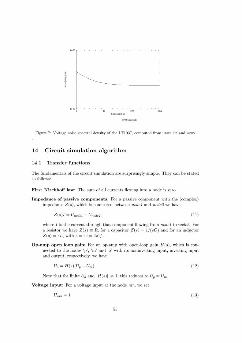
1e-09
1e-08
1 10 100 1000
Noi
se [V
/sqr
t(H
z)]
Frequency [Hz]
OP UNoise(op1)
Figure 7: Voltage noise spectral density of the LT1037, computed from un=2.5n and uc=2
.
14 Circuit simulation algorithm
14.1 Transfer functions
The fundamentals of the circuit simulation are surprisingly simple. They can be statedas follows:
First Kirchhoff law: The sum of all currents flowing into a node is zero.
Impedance of passive components: For a passive component with the (complex)impedance Z(s), which is connected between node1 and node2 we have
Z(s)I = Unode1 − Unode2, (11)
where I is the current through that component flowing from node1 to node2. Fora resistor we have Z(s) ≡ R, for a capacitor Z(s) = 1/(sC) and for an inductorZ(s) = sL, with s = iω = 2πif .
Op-amp open loop gain: For an op-amp with open-loop gain H(s), which is con-nected to the nodes ‘p’, ‘m’ and ‘o’ with its noninverting input, inverting inputand output, respectively, we have
Uo = H(s)(Up − Um) (12)
Note that for finite Uo and |H(s)| 1, this reduces to Up ≈ Um.
Voltage input: For a voltage input at the node nin, we set
Unin = 1 (13)
55

Current input: For a current we set
Iin = 1. (14)
In the special case of a floating voltage input, the equation is
Unin − Unin2 = 1, (15)
where nin represents the input node and nin2 the second input node of a floatingvoltage input.
Mutual inductances These are not so obvious. The procedure is as follows ([7,section 2.2.4]): If two coils L1 and L2 are coupled with the coupling factor k12(0 ≤ k12 ≤ 1), a mutual inductance M12 with the unit Henry is computed as
M12 = k12√L1L2. (16)
In the equation for L1, which normally states something like
sL1 IL1 − Unode1 + Unode2 = 0, (17)
an additional term +sM12 IL2 is introduced. Correspondingly, in the equationfor L2, the term +sM12 IL1 is added.
We find that for each component we get one equation and one unknown (the currentthrough that component). For each node, we also get one equation and one unknown(the voltage at that node). Furthermore, for the input we have one extra equation andalso an extra unknown (the input current Iin). All these equations are linear in theunknowns. This can most easily be demonstrated with an example, again using thelow-pass filter of Figure 1 on page 15. We obtain the following equations20:
20 In the present version of LISO, these equations (with numerical values substituted) can be printedby the program for debugging purposes. To do so, disable any fitting instructions and enter a freqinstruction likefreq lin 1k 1k 0
i.e. enter 0 ‘steps’ to request the debugging output, and set both start- and stop-frequency to thefrequency of interest.
56

1
sC2IC2 − Unsum = 0 (C2)
1
sC5IC5 − Uno + Unm = 0 (C5)
1
HOP1(s)Uno + Unm = 0 (OP1)
R1IR1 − Unin + Unsum = 0 (R1)
R3IR3 + Unsum − Uno = 0 (R3)
R4IR4 − Unsum + Unm = 0 (R4)
R6IR6 − Unin = 0 (R6)
−IR1 − IR6 + Iin = 0 (nin)
−IC2 + IR1 + IR3 − IR4 = 0 (nsum)
−IC5 + IOP1 − IR3 = 0 (no)
IC5 + IR4 = 0 (nm)
Unin = 1 (input)
(18)
These are 12 linear equations for the 12 unknown variablesIC2, IC5, IOP1, IR1, IR3, IR4, IR6,Unin, Unsum, Uno, Unm and Iin.
Note that for a current input, the first 11 equations remain unchanged and the lastone is replaced by Iin = 1. This basic set of equations is already sufficient to computethe currents through all components and the voltages at all nodes. All results listed as“transfer functions” in section 7.1 on page 23 can be obtained from this set of equations.
14.1.1 Transmission lines
n4 n6
u1 u2
i1
i1
i2
i2
n3 n5
Figure 8: A transmission line.
The model for transmission lines is taken from Ref. [?, Section 2.1.5]. Referring toFigure 8, we have:
U1 = U2 cosh γl + I2Z sinhγl,
I1 =U2Z
sinhγl + I2 cosh γl, (19)
57

with l the physical length of the transmission line,
Z =
√R′′ + sL′
G′ + sC ′, (20)
γ =√(R′′ + sL′)(G′ + sC ′), (21)
s = iω = 2π i f, (22)
R′′ = R′
√1 +
f
fskin. (23)
The LISO paramaters for a transmission line are (see Section 6.5 on page 18):l, Z0, R
′, C ′, G′ and fskin.Z0 is only used to compute L′ according to
L′ = Z20C′. (24)
The series loss resistance of the line, R′′l, increases with frequency due to the skin effect[?, 2.1.4], beginning at the limiting frequency fskin, which is usually a few kHz.
Other frequency-dependent effects, in particular a frequency dependence of C ′ or G′
do exist, but depend on the particular type of transmission line and are therefore notincluded in this model.
Using
U1 = U3 − U4, U2 = U5 − U6, (25)
and the abbreviations
sx = sinh γl, cx = cosh γl, (26)
For LISO, equation (19) is rewritten as
−Z I1 +cxZ I2 +sxU5 −sxU6 = 0 ,+sxZ I2 −U3 + U4 +cx U5 −cx U6 = 0 .
(27)
These are the two equations added to the linear system for each transmission line,according to the two new variables I1 and I2. Furthermore the currents I1 and I2 areadded with the appropriate sign to the four equations that described the nodes n3, n4,n5 and n6.
14.2 Noise calculations
It turns out that a set of linear equations very similar to the one above can be usedto compute the noise, if we now interpret all voltages and currents as linear spectraldensities. We introduce noise sources into the circuit, as described below, and computethe voltage at a certain node, interpreted as linear spectral noise density. All compo-nent characteristics and Kirchhoff’s law remain valid. We must, however, take care tocompute only one noise source at a time, and then quadratically add the results. Oth-erwise different noise sources might be added with a complex phase, or even subtracted,whereas we want to treat all noise sources as independent and uncorrelated. Further-more we only use the absolute value of the computed noise voltage, and not its phase,and hence the sign with which we introduce the noise source becomes unimportant.
58

14.2.1 Treatment of the input
As mentioned above, the input is treated differently for noise calculations. The lastequation is replaced by
IinZin + Uinput−node = 0 (28)
for the case of normal inputs and
IinZin + Uinput−node − Uinput−node2 = 0 (29)
for a floating voltage input. This corresponds to the impedance Zin connected betweenthe input nodes.
14.2.2 Resistor noise
The equation describing a resistor,
RI − Unode1 + Unode2 = 0, (30)
is replaced by
RI − Unode1 + Unode2 = Un, (31)
where Un is the Johnson noise expressed as voltage noise source, Un =√4kTR. This
corresponds to connecting the noise source Un in series with the resistor:
Note that as compared with the equations above, the right hand side is now changed,we still have the same unknowns and left-hand sides, but different right hand sides.The desired result is the voltage at a certain node, interpreted as linear spectral noisedensity.
14.2.3 Op-amp voltage noise
To compute the contribution of the voltage noise of an op-amp, we replace the equationdescribing the op-amp
Uo = H(s)(Up − Um) (32)
by
Uo = H(s)(Up − Um + Un). (33)
This corresponds to amplifying not only the differential input voltage, but also theadditional (equivalent input noise) voltage Un (see Figure 9 on the following page).
59
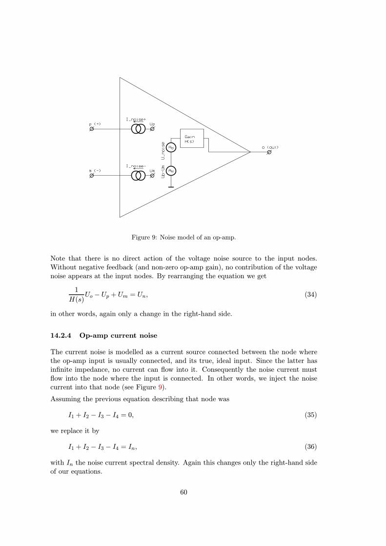
Figure 9: Noise model of an op-amp.
Note that there is no direct action of the voltage noise source to the input nodes.Without negative feedback (and non-zero op-amp gain), no contribution of the voltagenoise appears at the input nodes. By rearranging the equation we get
1
H(s)Uo − Up + Um = Un, (34)
in other words, again only a change in the right-hand side.
14.2.4 Op-amp current noise
The current noise is modelled as a current source connected between the node wherethe op-amp input is usually connected, and its true, ideal input. Since the latter hasinfinite impedance, no current can flow into it. Consequently the noise current mustflow into the node where the input is connected. In other words, we inject the noisecurrent into that node (see Figure 9).
Assuming the previous equation describing that node was
I1 + I2 − I3 − I4 = 0, (35)
we replace it by
I1 + I2 − I3 − I4 = In, (36)
with In the noise current spectral density. Again this changes only the right-hand sideof our equations.
60
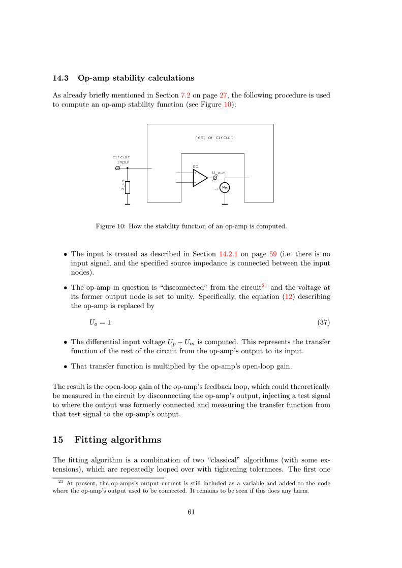
14.3 Op-amp stability calculations
As already briefly mentioned in Section 7.2 on page 27, the following procedure is usedto compute an op-amp stability function (see Figure 10):
Figure 10: How the stability function of an op-amp is computed.
• The input is treated as described in Section 14.2.1 on page 59 (i.e. there is noinput signal, and the specified source impedance is connected between the inputnodes).
• The op-amp in question is “disconnected” from the circuit21 and the voltage atits former output node is set to unity. Specifically, the equation (12) describingthe op-amp is replaced by
Uo = 1. (37)
• The differential input voltage Up −Um is computed. This represents the transferfunction of the rest of the circuit from the op-amp’s output to its input.
• That transfer function is multiplied by the op-amp’s open-loop gain.
The result is the open-loop gain of the op-amp’s feedback loop, which could theoreticallybe measured in the circuit by disconnecting the op-amp’s output, injecting a test signalto where the output was formerly connected and measuring the transfer function fromthat test signal to the op-amp’s output.
15 Fitting algorithms
The fitting algorithm is a combination of two “classical” algorithms (with some ex-tensions), which are repeatedly looped over with tightening tolerances. The first one
21 At present, the op-amps’s output current is still included as a variable and added to the nodewhere the op-amp’s output used to be connected. It remains to be seen if this does any harm.
61

is the Nelder-Mead Simplex algorithm [1], a very robust geometrical algorithm whichis good at approaching a minimum from far-off starting values. Secondly there is theLevenberg-Marquardt algorithm which is much faster once the vicinty of the (or a) min-imum has been found. The author has learned about these algorithms and their properapplication from his father Gunther Heinzel, who has been using such algorithms forpharmacocinetic applications for many years.
15.1 Extensions to the Nelder-Mead Simplex algorithm
The algorithm is well described in the original paper[1]. It is implemented in LISO asdescribed there. The only extension is the computation of start vectors:
15.1.1 Computation of n+ 1 directions equally distributed in Rn
In order to start the algorithm to minimize a function of n parameters, we need n+ 1points in Rn. However, in our application only one initial guess is given. The same istrue when the algorithm is restarted after apparent convergence to one point, whichis urgently recommended because the simplex possibly has degenerated and no longerspans the whole parameter space.
Here a set of (n+1) unity vectors v0, . . . , vn, distributed as regularily as possible in Rn
is useful. The problem has a unique solution (except for rotations) and the coordinatesof the resulting points can explicitly be calculated by
v0 = (1, 0, . . . , 0)
v1 = (b0, a1, 0, . . . , 0)
v2 = (b0, b1, a2, 0, . . . , 0)
. . .
vi = (b0, . . . , bi−1, ai, 0, . . . , 0)
vn−1 = (b0, . . . , bn−2, an−1)
vn = (b0, . . . , bn−2, bn−1)
(38)
with the diagonal elements
aj =
√(n+ 1)(n− j)
n(n− j + 1); (a0 = 1) (39)
and the subdiagonal elements
bj = −
√(n+ 1)
n(n− j + 1)(n− j)=
ajj − n
; (b0 = −1
n) (40)
Any two different vectors of this set have the scalar product
vi · vk = cos∠(vi, vk) = −1
n(41)
and the distance |vi − vk| =√2 + 2/n
62

15.1.2 Derivation
The basic observation is that (n+1) equally distributed points cannot be given directlyin Rn, but easily in Rn+1: (1, 0, 0, . . . , 0), (0, 1, 0, . . . , 0), . . . , (0, 0, . . . , 0, 1). They all liein the n-dimensional affine subspace x = (x0, . . . , xn) ∈ Rn+1 | x0+x1+ · · ·+xn = 1.By subtracting (1/(n+1), 1/(n+1), . . . , 1/(n+1)) and normalizing, new unity vectorsare obtained, now all in the linear subspace H = x ∈ Rn+1 | x0 + x1 + · · · + xn = 0.Now the scalar product given above can readily be calculated, and the coordinates canbe found either by constructing an orthonormal base of H and transforming the points’coordinates into this new base, or by computing the Cholesky–decomposition of the(n+ 1)× (n+ 1)–matrix
S =
1 −1/n −1/n . . .
−1/n 1 −1/n . . .
. . .. . .
−1/n . . . −1/n 1
(42)
15.1.3 Example
For n = 3 we get the 4 corners of a tetrahedron with center 0 and all points on theunity sphere:
( 1, 0, 0 )
(−13 ,23
√2, 0 )
(−13 , −13
√2,
√23 )
(−13 , −13
√2, −
√23)
(43)
15.1.4 Initialization and termination
Whenever the Simplex algorithm is called, it re-initializes the simplex by adding afraction of the above unity vectors to the given inital estimate. The fraction (calledstarting length) is controlled by the overall minimization strategy (see Section 15.3 onpage 66). In order to span all directions in parameter space as equally as possible,the unity vectors are randomly shuffled before each call of the Simplex algorithm. Thealgorithm then proceeds as usual. It is terminated as soon as the relative difference inχ2 between the best and worst points in the present simplex falls below a certain limit(called tolerance), which is also controlled by the overall minimization strategy.
Note that the initial simplex does not contain the single point that was given as previousbest estimate. Consequently in the first few iterations of the Simplex algorithm, theχ2 may be worse than at the previous best point. This effect may look disturbing, butin my experience this procedure is more likely to escape from local minima in complexproblems. If the previous best estimate was already the global minimum, the simplexjust shrinks more or less symmetrically to that point and eventually reproduces theprevious best χ2.
63

15.2 Extensions to the Levenberg-Marquardt algorithm
15.2.1 Numerical derivatives
Since the Levenberg-Marquardt algorithm requires the derivatives of χ2 with respectto the parameters, and χ2, which results from the simulation, cannot be differentiatedanalytically, we use the following approximations for numerical derivatives:
∂f
∂x≈
f(x+ h)− f(x− h)
2h, (44)
∂2f
∂x2≈
f(x+ h)− 2f(x) + f(x− h)
h2, (45)
∂2f
∂x∂y≈
f(x+ h, y + h)− f(x+ h, y − h)− f(x− h, y + h) + f(x− h, y − h)
4h2.
(46)
The problem of selecting a suitable stepwidth h is simplified by the fact that the mini-mization takes place with the logarithms of all parameters, such that a fixed stepwidthh is usually appropriate. In the present implementation this h is a constant namedDERIV H read from fil.ini with the default value of 10−3, corresponding to a 0.1%variation of the physical parameter. Note that any inaccuracy in the derivatives mayaffect the speed of convergence of the Levenberg-Marquardt algorithm, but not thefinal result.
15.2.2 Application to complex data
In a standard implementation of the Levenberg-Marquardt algorithm (see e.g. [2]), thegradient and Hessian of χ2 with respect to the parameters are expressed by
βk = −1
2
∂χ2
∂pk,
αkl =1
2
∂2χ2
∂pk∂pl,
(47)
where pk is the k-th parameter and χ2 is defined in equation (7). For brevity we define
zi = yi − y(fi, p1, . . . , pm),
zk+i = yi − y(fi, p1, . . . , pk + h, . . . , pm),
zk−i = yi − y(fi, p1, . . . , pk − h, . . . , pm)
(48)
and thus have
χ2 =∑i
wi |zi|2 . (49)
64

Note that in our case zi is complex, different from standard implementations of theLevenberg-Marquardt algorithm. Using the approximation (44) we thus find for thefirst derivatives
∂χ2
∂pk=∑i
wi∂
∂pk|zi|
2 =∑i
wi
∣∣∣zk+i ∣∣∣2 − ∣∣∣zk−i ∣∣∣22h
, (50)
βk =∑i
wi
∣∣∣zk−i ∣∣∣2 − ∣∣∣zk+i ∣∣∣24h
. (51)
For the second derivatives we find
∂2χ2
∂pk∂pl=∑i
wi∂2
∂pk∂pl|zi|
2
=∑i
wi∂2
∂pk∂pl(zi z
∗i )
=∑i
wi
(∂z∗i∂pk
∂zi∂pl
+∂zi∂pk
∂z∗i∂pl
+ z∗i∂2zi∂pk∂pl
+ zi∂2z∗i∂pk∂pl
) (52)
At this point the last two terms in the parenthesis are dropped with the followingreasons: The computational efficiency increases (we need only nparam evaluations ofequation (44) instead of n2param evaluations of equation (46)) and empirical evidence[2, 3] indicates that dropping these terms yields equally good results or even improvednumerical stability. Furthermore, zi should be small near the minimum of χ2 and havea zero average. Finally, errors in αkl and βk affect only the speed of convergence, butnot the final result. Now we apply equation (44) and obtain
∂2χ2
∂pk∂pl≈∑i
wi4h2
[((zk+i )∗ − (zk−i )∗
)(zl+i − zl−i
)+(
zk+i − zk−i
)((zl+i )∗ − (zl−i )∗
)]=∑i
wi2h2[((zk+i )∗ − (zk−i )∗
)(zl+i − zl−i
)]=∑i
wi2h2
([zk+i − zk−i ][zl+i − zl−i ] + [zk+i − zk−i ][zl+i − zl−i ]
),
αkl =∑i
wi4h2
([zk+i − zk−i ][zl+i − zl−i ] + [zk+i − zk−i ][zl+i − zl−i ]
).
(53)
For k = l the last expression simplifies to
αkk =∑i
wi4h2
∣∣∣zk+i − zk−i
∣∣∣2 . (54)
The function derivs2 computes βk and αkl from equations (51) and (53). For debug-ging purposes, there is another function truederivs that uses the definining equations(7) and (47) together with (44)–(46) to compute the same quantities.
65

15.2.3 λ search
Now that we have found A = (αkl) and b = (βk) the algorithm proceeds as usual. Weconstruct the augmented matrix
A′(λ) =(α′kl(λ)
)with
α′kk(λ) = (1 + λ)αkk,
α′kl(λ) = αkl (k = l),
(55)
solve the set of linear equations
A′d = b (56)
for the corrections d(λ) = (δk(λ)), add the corrections δk to the parameters pk andrecompute χ2(λ). Because the computation of A is comparatively expensive, our strat-egy to control λ differs from the standard procedure. After each computation of A,we scan λ in steps of 1.5 (MAR LAMFACT), starting with λ = 10−3 (MAR LAMSTART), withlimits 10−8 (MAR LAMMIN) and 1000 (MAR LAMMAX), until we have found the value of λthat minimizes χ2(λ). Then we recompute A and b and start a new scan of λ. Thisprocedure is repeated until the relative improvement in χ2 becomes less than 10−3
(MAR REPTOL).
Note that if constraints are violated, the χ2 function used in the λ search is increaseddue to the ‘punishment function’ (see 15.4 on the next page), whereas A and b areunaffected by the constraints. In this situation the Marquardt algorithm will usuallyfail and return with no improvement, leaving the work to the Simplex algorithm.
15.3 Overall minimization strategy
At present the following strategy is implemented: The main loop first calls the Sim-plex algorithm with a tolerance of 10−2 (SIM STARTTOL) and a length factor of 0.4(SIM STARTLEN). Then the Marquardt algorithm is called, after which it loops back tothe Simplex algorithm. Each time the Simplex algorithm is called, the length factor isdivided by 3.3 (SIM LENFACT) and the tolerance by 10 (SIM TOLFACT). The optimizationis always ended after a Simplex step, such that normally the minimum course of eventsis Simplex–Marquardt–Simplex. The criterion for ending is a relative improvement inχ2 below 10−4 (ENDTOL) in the last Simplex step. There is, however, a shortcut forvery good fits (which usually occur with simulated but almost never with measureddata): If after the Marquardt algorithm χ2 is below 10−5 (MAR QUICKOUT), the itera-tion is stopped immediately. This feature can be disabled by setting (MAR QUICKOUT)to a very small number (e.g. 10−13 or so) in the file fil.ini.
Because the parameters may differ widely in magnitude (e.g. pF vs. MΩ), all opti-mization algorithms work with the logarithms of the parameters. A consequence isthat only positive parameters are allowed. The transformed parameters now all have arange of approximately −20 . . . 20 or a subset thereof, with a precision of 0.001 beingadequate for most purposes. This transformation is essential for the efficiency and reli-ability of both the Simplex and the Marquardt algorithm, which have some geometricalbackground.
66

15.4 Implementation of parameter limits
There are at least three possibilities to implement limits for the parameters:
• With a transformation such as a suitably scaled arctan(x) function new parame-ters can be introduced which may vary between −∞ and ∞. The possible hugevalues of the transformed parameters might, however, upset geometrical algo-rithms.
• Any proposed set of new parameters can be examined for crossing the limits, andthen approporiate action may be taken, such as clipping at the limits. This isa possible approach, but rather complicated to implement into already complexalgorithms.
• The function to be minimzed, χ2, may be modified such that a “penalty” is addedwhenever the limits are crossed.
Since this last possibility (penalty function) is the most flexible22 one, is easy to imple-ment and has proven very satisfactory so far, it was chosen for LISO.
The penalty function was chosen as follows: Define
f(x) =
exp(x)− x− x2/2; x > 01; x ≤ 0
(57)
with f(x) ≡ 1 for x < 0, f(1.57) ≈ 2, f(x) increasing rapidly for x > 0 and twicedifferentiable at x = 0. Now consider the parameter pi with limits mini and maxi.Here parameters and limits are taken directly with their physical values (i.e. neitherscaled nor as logarithms). If pi falls outside mini or maxi, compute x > 0 as follows:
x =
(pi/maxi)− 1; pi ≥ maxi(mini/pi)− 1; pi ≤ mini
(58)
Then multiply x by 1.57/α, where α has been precomputed as
α =
β; maxi /mini > 2β(maxi/mini)− 1; maxi /mini ≤ 2
(59)
with the constant β = 0.1 (PUNISH BETA in the initialization file).
The function χ2 is then multiplied with f(x) for all parameters which exceed theirlimits. The effect is that χ2 is doubled if pi has passed beyond a limit by 10% (of thatlimit), with the “10%” being reduced if mini and maxi are close together.
A related strategy (still experimental) is used for the mininput instruction. For all datapoints with fmin ≤ f ≤ fmax, the allowable input signal Sa is computed (in the sameway as for the maxinput instruction) and compared to the required signal Sr (which
22It is, for example, possible to implement more complex constraints very easily.
67

was given by the user in the mininput instruction). If Sa < Sr, the following sum isincremented:
a =∑Sa<Sr
logSrSa
. (60)
After looping over all data points, a has a value between 0 (for no constraint violation)and a few thousand (for heavy constraint violation in many data points). This value ais then transformed by
b = 20arctan(a/10), (61)
which is linear for small a, monotonuously increasing and limited to 10π. The previousχ2 is then multiplied by exp(b). If the computed transfer function agrees perfectly withthe data file, χ2 is very close to zero and the multiplication by exp(b) was found toprovide not enough ‘punishment’ in some cases. Hence the modified χ2 is set to
χ2mod = min(χ2 exp(b), b). (62)
The χ2 thus modified is used for the Simplex algorithm and the λ search of the Mar-quardt algorithm. The gradient and Hessian for the Marquardt algorithm (equation 47on page 64) as well as the variance–covariance matrix (see Section 15.5) are not affectedby the limits. This means that if one or more parameters are constantly running againsta limit, the Marquardt algorithm may be not working and convergence to a minimummay then rely only on the Simplex algorithm.
If that final minimum of the modified χ2 involves a parameter having crossed its limit,the correlation matrix and confidence limits (see Section 15.5) may be wrong, becausewe are not at a minimum of the unmodified χ2.
15.5 Correlation matrix and confidence limits
After the fit has converged, the matrix A = (αkl) is computed according to equation 53on page 65 and inverted to give the variance–covariance matrix
C = (ckl) = A−1. (63)
The correlation between two parameters pk and pl is now computed as
corrkl =ckl
√ckk cll
. (64)
The standard deviation σk of pk is computed as
σk =
√χ2 ckk
ndata − nparam. (65)
This standard deviation refers to the logarithmic parameter and is transformed backinto physical parameters by
re = exp(σk)− 1 (66)
68

where re now means the relative error in the parameter. Note that for σi ≥ log 2 ≈ 0.69the relative error re becomes equal or bigger to the best estimate of the parameterbecause
log(pbest)− σi ≤ log pi ≤ log(pbest) + σi, (67)
which at the limit σi = log 2 transforms into
0.5 pbest ≤ pi ≤ 2 pbest. (68)
“Standard deviations” such big (or bigger) are only of very limited usefulness anyway.Note also that both correlation matrix and confidence limits may be wrong, if the finalminimum of χ2 involves any parameter having crossed its limit (see Section 15.4 onpage 67).
16 Implementation notes
16.1 Internal scaling
For most numerical algorithms, it is advantageous or even necessary to scale the vari-ables, i.e. to express them in some kind of natural unit instead of their SI units. Thisis in particular true in LISO, where we deal with e.g. pF and MΩ, nA and MHz. Thepurpose is to get internal variables that have at least comparable orders of magni-tude. Without such scaling, many algorithms may become imprecise, inefficient or mayeven fail. In LISO, the following internal scaling is used for impedances, capacitances,inductances, voltages, currents and frequencies:
R = R′Rn (69)
C = C ′Cn (70)
L = L′ Ln (71)
U = U ′ Un (72)
I = I ′ In (73)
f = f ′ fn. (74)
Here R (as an example) stands for the real physical values of the impedance (with theunit Ω), R′ is the internal value used by LISO algorithms (without any unit), and Rnrepresents the scale factor (again with the unit Ω). Out of various possibilities to selectreasonable scale factors, LISO uses the following one:
Rn = Rmean (75)
Cn = Cmean (76)
Ln = R2nCn (77)
Un = 1V (78)
In = Un/Rn (79)
fn = 1/(Rn Cn), (80)
69

where Rmean and Cmean are the geometric mean values of all resistors and capacitors inthe circuit, respectively. Another possibility, which might even be better for computa-tional purposes, but which would make the program more complex, would be to choosefn equal to the frequency just being considered, and choose the other scale factorsaccordingly. For simplicity we have, however, chosen the above scale factors, whichremain constant for any single run of LISO. The numerical values of the scale factorsare printed at the end of the output file.
16.2 Sparse matrices
For each frequency, a system of linear equations (such as equation (18)) needs to besolved numerically. Even for circuits of moderate complexity, that system gets alreadyrather large (its dimension is: number of components + number of nodes +1). Ofcourse it is possible to apply standard techniques, such as LU-decompositon. However,the computation time required makes that approach very impractical (in particularfor the fitting function, which needs to solve the system many times). It turns out,however, that most elements of the matrix describing the system are zero. Such matricesare called sparse, and there are special techniques available to deal with them. LISOuses a package called SPARSE [4], which was developped for circuit simulation and istherefore very well suited for this application. Practically, on a “normal” computer, atleast the fitting function of LISO would be unusably slow without such a specializedsparse matrix package.
16.3 Efficient noise computation using the transposed matrix
In one run of LISO, the noise is computed only at one fixed node. Usually, several or allnoise contributions are to be computed simultaneously. If we write the linear system(18) in matrix form, we get
Ax = b (81)
with A the matrix describing the left-hand sides of (18), b the right-hand sides andx the solution vector (consisting of all voltages and currents in the circuit). Formalinversion yields
x = A−1b. (82)
We are only interested in one component of x, say xn, which we call y (a scalar):
y = xn = (A−1b)n. (83)
The index n represents the node of interest in the solution vector and is fixed. Asexplained in Section 14.2, every noise contribution corresponds to a different right-hand-side vector b, say
bj = kjej (84)
70

with kj some real constant and ej the unity vector (0, . . . , 1, . . . , 0) with the ‘1’ atposition j. So the jth noise contribution can be computed as
yj = (A−1bj)n = kj(A−1ej)n. (85)
If more than one noise contribution is to be computed, we need to separately computeeach of them and then add them quadratically:
U =
√∑j
|yj|2, (86)
a nonlinear operation. (As explained in Section 14.2, we cannot directly computedifferent noise contributions in one operation). In a straightforward approach, wewould have to evaluate equation (82) separately for each bj given by (84), an obviouslyinefficient procedure. We can, however, rewrite equation (85) as follows:
yj = kj∑l
(A−1)nl(ej)l = kj(A−1)nj. (87)
We see that all the different noise contributions are contained in one row (with index n)of the matrix A−1. We can compute that row in one operation if we solve the equation
Aty = en, (88)
where At represents the transpose of A. The elements of y can be thought of as transferfunctions from the various points where noise sources might reside to the specified nodewhere the noise is to be computed. Then we can immediately compute
yj = kj yj (89)
and apply (86).
17 Application examples
In this Section, several simple examples are presented to help the reader understandthe possibilities of LISO and the necessary input. They are not intended to exhaust allof LISO’s possible uses. They are sorted by increasing complexity.
17.1 Root mode simulation
The aim is to compute the frequency response of a 4-pole Tschebyscheff filter with 3 dBripple, a corner frequency of 4 kHz and a DC-gain of 10. From filter tables[6, 5], weobtain the following pole data:
Stage 1: Ω = 0.44265, Q = 1.0765Stage 2: Ω = 0.9503, Q = 5.5770
Now all we need is a frequency scaling (from 1Hz to 4 kHz) and a gain scaling (from 1to 10). The input file ex1.fil is:
71

pole .44265 1.0765 # from filter tables
pole .9503 5.577 # from filter tables
ffactor 4000 # frequency factor
factor 10 # gain factor
tfoutput db:deg-
freq log 100 100k 400
gnuterm eps
gnuterm x11
Note the use of the deg- coordinate specifier (see Section 7.1.2 on page 23) in order toavoid an ugly phase jump at 180. The resulting plot is shown in Figure 11.
-120
-100
-80
-60
-40
-20
0
20
40
100 1000 10000 100000
-315
-270
-225
-180
-135
-90
-45
dB
Pha
se [D
egre
e]
Frequency [Hz]
TF dB TF Phase
Figure 11: Example 1: Frequency response of a 4-pole Tschebyscheff filter.
17.2 Root mode fit
The transfer function of a suspended pendulumwas measured with a spectrum analyzer.(These are real experimental data, the transfer function is from a current in a coil tothe actual movement of the penulum, measured optically.) It has the general form of atwo-pole low-pass filter:
HP(s = i f) =AP
1 +s
fPQP+
s2
f2P
(90)
We want to find the pole frequency fP, its associated QP and the overall gain factorAP. The data from the spectrum analyzer was stored in the file called ex2.dat. Itconsists of 3 columns: first the frequency (in Hz), second the real part and third theimaginary part of the transfer function. The frequency runs from 0 to 100Hz in 801steps. The input file ex2.fil is:
72

pole 1.5 2 # pole at f=1.5 Hz with Q=2
factor -10 # overall factor is negative
freq log 0.1 100 400
tfoutput abs:deg
param pole0:f 0.1 10
param pole0:q 0.1 10
param factor 1 100 # note the factor used for fitting is positive!
fit ex2.dat reim rel plotfirst
gnuterm eps
gnuterm x11
Note that the overall factor is negative. Its starting value (defined by the instructionfactor -10) must be negative in this case, because the fitting algorithm cannot “cross”from negative to positive values and vice versa. The limits in the param instruction aswell as intermediate values in the printout are positive. The overall factor in root modeis the only parameter in LISO that can have negative values and has this peculiar be-haviour. All other parameters are always positive. The instruction fit ex2.dat reim
rel plotfirst gives the filename, file format and weighting. The option plotfirst
requests a plot of the function with the startvalues as well as one with the final fittedvalues. Note also that the resulting plot (shown in Figure 12 on the next page) hasa logarithmic x-axis and the coordinates abs:deg, although the data file has linearlyspaced x-values and the coordinates reim. The first data point at the frequency 0Hzcannot be plotted. Running LISO on this example yields the following output:
nfunk Stat ssq pole0:f pole0:q factor
1 Start 1924 1.5 2 10
5 Splx 243.2 1.242 1.443 8.752
7 Splx 32.69 800.1m 2 12.49
17 Splx 27.13 990.7m 2.32 9.693
21 Splx 24.39 883.3m 1.963 10.96
34 Sout 22.28 898.4m 2.848 11.16
34 M in 22.28 898.4m 2.848 11.16
54 Marq 22.12 912.3m 2.954 10.69
54 M in 22.12 912.3m 2.954 10.69
64 Marq 22.12 913.5m 2.955 10.66
64 Mout 22.12 913.5m 2.955 10.66
68 Splx 35.06 913.5m 2.955 12.04
70 Splx 25.62 949m 2.955 10.52
78 Splx 22.72 900.2m 2.929 10.68
100 Sout 22.14 910.4m 2.976 10.78
Correlation matrix
pole0:f pole0:q factor
pole0:f 1
pole0:q 0.169 1
factor -0.973 -0.183 1
73

Best parameter estimates:
pole0:f = 913.50261m +- 11.48m (1.26%)
pole0:q = 2.955091 +- 227.8m (7.71%)
factor = -10.663409 +- -277.8m (2.6%)
Note that the final minimum of SSQ is already found by the first application of theMarquardt algorithm (after 64 function evaluations). The subsequent call of the Sim-plex algorithm cannot improve this minimum. The final results are always the best onesever found during the whole fitting procedure. The printed “deviations” of the bestparameter estimates have no real meaning, unless the data have normally distributederrors and these errors are known and entered (which is not the case in this example).The correlation matrix is, however, still valid.
0.0001
0.001
0.01
0.1
1
10
100
0.1 1 10 100-45
0
45
90
135
Abs
Pha
se [D
egre
e]
Frequency [Hz]
ex2.dat Abs ex2.dat Phase
TF(start) Abs
TF(start) Phase TF(fitted) Abs
TF(fitted) Phase
Figure 12: Example 2: Fitting a measured frequency response to a 2-pole lowpass filter model.
References
[1] J. A. Nelder, R. Mead: A simplex method for function minimization, ComputerJournal 7 (1965), 308–313
[2] William H. Press, Saul A. Teukolsky, William T. Vetterling, Brian P. Flannery:Numerical Recipes in C, The Art of Scientific Computing, Cambridge UniversityPress, 2nd ed., 1992.
[3] J. R. Donaldson, R. B. Schnabel: Technometrics 29 (1987), 67–82
[4] SPARSE: A Sparse Linear Equation Solver, Version 1.3a, 1 April 1988, by KennethS. Kundert and Alberto Sangiovanni-Vincentelli, Department of Electrical Engi-
74

neering and Computer Sciences, University of California, Berkeley, Calif. 94720;available from http://www.netlib.org/sparse/
[5] M. Herpy, J.–C. Berka: Aktive RC–Filter, Franzis–Verlag Munchen 1984
[6] L. v. Wangenheim: Aktive Filter in RC– und SC–Technik, Huthig–Verlag Heidel-berg 1991
[7] E. E. E. Hoefer, H. Nielinger: SPICE – Analyseprogramm fur elektronische Schal-tungen, Springer–Verlag 1985
[8] S. Brandt: Datenanalyse, B.I. Wissenschaftsverlag 1992
[Horowitz–Hill] P. Horowitz, W. Hill: ‘The Art of Electronics’, 2. ed., Cambridge Uni-versity Press 1989.
75