LiquidityAdjustedIntradayValueatRisk - iaeng.org · pt `ASK t wherert denotestherawlogVWAP-returnsand`t the deterministic seasonality pattern of intraday volatility. We ﬁrst chose

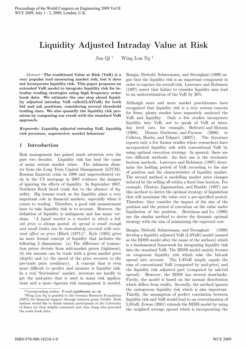
Liquidity Adjusted Intraday Value at RiskJun Qi ∗ Wing Lon Ng †

Abstract—The traditional Value at Risk (VaR) is avery popular tool measuring market risk, but it doesnot incorporate liquidity risk. This paper proposes anextended VaR model to integrate liquidity risk for in-traday trading strategies using high frequency orderbook data. We estimate the one step ahead liquid-ity adjusted intraday VaR called(LAIVaR) for bothbid and ask positions, considering several thresholdtrading sizes. We also quantify the liquidity risk pre-mium by comparing our result with the standard VaRapproach.

Keywords: Liquidity adjusted intraday VaR, liquidityrisk premium, asymmetric market behaviour

1 Introduction

Risk management has gained much attention over thepast two decades. Liquidity risk has lead the causeof many serious market crises. The infamous disas-ter from the Long Term Capital Management (LTCM),Russian financial crisis in 1998 and unprecedented cri-sis in the US mortgage in 2007 evidence the dangersof ignoring the effects of liquidity. In September 2007,Northern Rock faced crash due to the absence of liq-uidity. Big lessons teach us the liquidity plays a veryimportant role in financial markets, especially when itcomes to trading. Therefore, a good risk measurementhave to take liquidity risk in to account. However, thedefinition of liquidity is ambiguous and has many ver-sions. “A liquid market is a market in which a bid-ask price is always quoted, its spread is small enoughand small trades can be immediately executed with min-imal effect on price (Black (1971))”. Kyle (1985) givesan more formal concept of liquidity that includes thefollowing 3 dimensions: (a) The difference of transac-tion prices deviate from mid-market prices (tightness),(b) the amount can be trade with a given market price(depth) and (c) the speed of the price recovers to thepre-trade price (resiliency). A concept that is evenmore difficult to predict and measure is liquidity risk.In a real “frictionless” market, investors are hardly toget the mid-price that is used in many risk applica-tions and a more rigorous risk management is needed.

∗Corresponding author. E-mail:[email protected]†Wing Lon Ng is grateful to the German Research Foundation

(DFG) for financial support through research grant 531283. Bothauthors would like to thank seminar participants at the Universityof Essex for their helpful comments and Jian Jiang who providedthe order book data.

Bangia, Diebold, Schuermann, and Stroughair (1999) ar-gue that the liquidity risk is an important component inorder to capture the overall risk. Lawrence and Robinson(1997) assert that failure to consider liquidity may leadto an underestimation of the VaR by 30%.

Although more and more market practitioners haverecognized that liquidity risk is a very serious concernfor firms, plenty studies have separately analyzed theVaR and liquidity. Only a few studies incorporateliquidity into VaR, not to speak of VaR at intra-day level (see, for example, Beltratti and Morana(1999), Dionne, Duchesne, and Pacurar (2006) orColletaz, Hurlin, and Tokpavi (2007)). The literaturereports only a few former studies where researchers haveincorporated liquidity risk with conventional VaR byusing optimal execution strategy. In general, there aretwo different methods: the first one is the stochastichorizon methods. Lawrence and Robinson (1997) deter-mine the holding period of VaR according to the sizeof position and the characteristics of liquidity market.The second method is modelling market price changesinduced by the selling off within a fixed time horizon. Forexample, Glosten, Jagannathan, and Runkle (1997) usethis method to derive the optimal strategy of liquidationthat will maximize the value over a pre-specified period.Therefore, they consider the impact of the size of theposition and the period of execution on the value underliquidation of the position. Bertsimas and Lo (1998)use the similar method to derive the dynamic optimalstrategy with the aim of minimizing the expected cost.

Bangia, Diebold, Schuermann, and Stroughair (1999)develop a liquidity adjusted VaR (LAVaR) model (namedas the BDSS model after the name of the authors) whichis a fundamental framework for integrating liquidity riskinto the standard VaR. The BDSS model mainly focuseson exogenous liquidity risk which take the bid-askspread into account. The LAVaR simply equals thesum of conventional VaR (computed by mid-price) andthe liquidity risk adjusted part (computed by ask-bidspread). However, the BDSS has several drawbacks:Firstly, the model is based on the normal distributionwhich differs from reality. Secondly, the method ignoresthe endogenous liquidity risk which is also important.Thirdly, the assumption of perfect correlation betweenliquidity risk and VaR would lead to an overestimation ofLAVaR. Erwan (2001) extends the BDSS model by usingthe weighted average spread which is incorporating the

Proceedings of the World Congress on Engineering 2009 Vol IIWCE 2009, July 1 - 3, 2009, London, U.K.

ISBN:978-988-18210-1-0 WCE 2009

endogenous risk effect to instead of the ask-bid spread.He also points out that the endogenous liquidity risk istaking one half part of the total market risk and mustnot be neglected.

Hisata and Yamai (2000) propose a framework for thequantification of LAVaR model that incorporates themarket impact induced by the trader’s own liquidation.They derive the optimal execution strategy according tolevel of market liquidity and the scale of the investor’s po-sition. They choose the holding period as an endogenousvariable and provide discrete time model and continuoustime model for LAVaR measurement.

Further, Agnelidis and Benos (2006) investigate intradayLAVaR in Athens Stock Exchange and extend the modelfrom Madhavan, Richardson, and Roomans (1997) by in-corporating trading volume and take both endogenousand exogenous liquidity risk into account. Their resultalso shows that the liquidity risk must not be neglected.Moreover, the LAVaR exhibits a U-shaped patternthroughout the day. In contrast, Giot and Gramming(2006) introduce a GARCH model to derive LAVaR inan automated auction market. Their empirical model isbased on the BDSS model and model the liquidity riskby calculating the weighted average bid price from thereal order book data. Their result shows that liquidity inVaR accounts significantly and the liquidity risk exhibitsan L-shape pattern throughout the day.

The motivation for our paper is as follows: Firstly, aswe claimed in the beginning that liquidity risk is a veryimportant fragment in whole risk system. However theconventional VaR models have not take the liquidity riskin to account. The conventional VaR models heavily relyon the implied assumption that an asset can be traded ata certain price at any quantity within a fixed period oftime. This assumption is not realistic under real marketconditions, especially in intraday trading, as execution isnot always guaranteed, i.e. the conventional VaR modelsnot capture the liquidity risk that traders are exposed to.This paper therefore attempts to measure additional riskdue to liquidity in the VaR using intraday data and ex-tends the existing literature in the following way. We con-sider the endogenous liquidity risk, taking into accountthe volume effect to model the liquidity adjusted intradayVaR (LAIVaR), which refers to the liquidity fluctuationdriven by the size of investors’ position.

Secondly, there is an asymmetry in up and down move-ment in the equity market.Down movement are typicallymore abrupt than up movement. This is relevant becauselike hedge funds maybe long assets and need a LAIVaRfor both long and short positions. In particular, we areinterested in differentiating between both bid and asksides since different market sides have to face differentprice movements as well. We estimate the one step aheadLAIVaR of both market sides providing to quantify their

real risk position.

The outline of the paper is as follows. Section 2 describesthe methodology and Section 3 presents the data and theempirical results. Section 4 concludes.

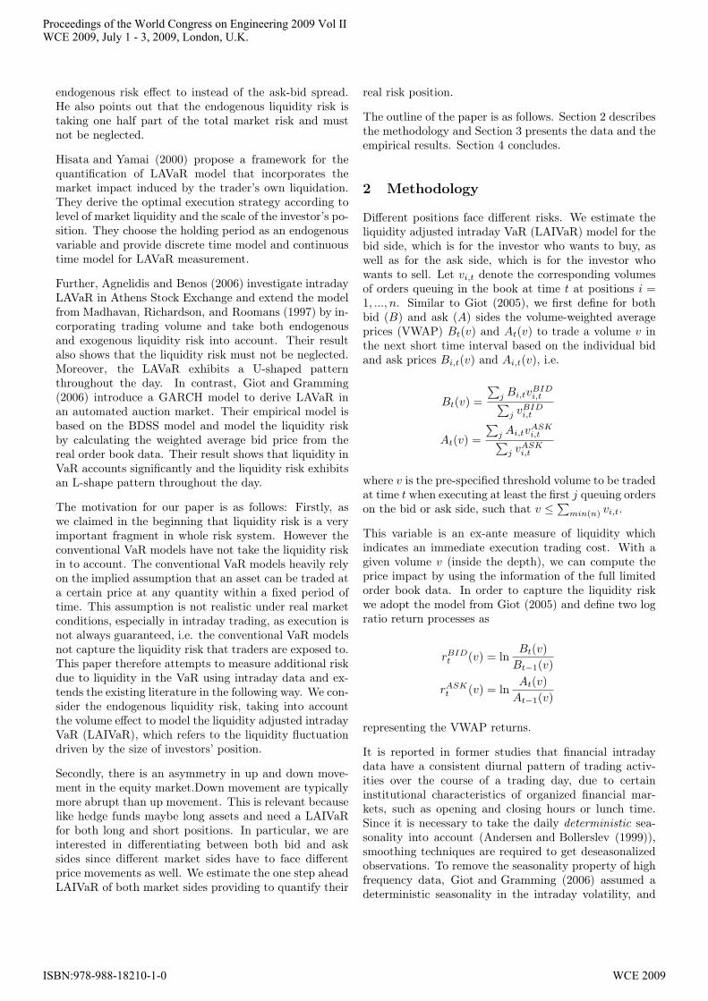
2 Methodology

Different positions face different risks. We estimate theliquidity adjusted intraday VaR (LAIVaR) model for thebid side, which is for the investor who wants to buy, aswell as for the ask side, which is for the investor whowants to sell. Let vi,t denote the corresponding volumesof orders queuing in the book at time t at positions i =1, ..., n. Similar to Giot (2005), we first define for bothbid (B) and ask (A) sides the volume-weighted averageprices (VWAP) Bt(v) and At(v) to trade a volume v inthe next short time interval based on the individual bidand ask prices Bi,t(v) and Ai,t(v), i.e.

Bt(v) =

∑j Bi,tv

BIDi,t∑

j vBIDi,t

At(v) =

∑j Ai,tv

ASKi,t∑

j vASKi,t

where v is the pre-specified threshold volume to be tradedat time t when executing at least the first j queuing orderson the bid or ask side, such that v ≤ ∑

min(n) vi,t.

This variable is an ex-ante measure of liquidity whichindicates an immediate execution trading cost. With agiven volume v (inside the depth), we can compute theprice impact by using the information of the full limitedorder book data. In order to capture the liquidity riskwe adopt the model from Giot (2005) and define two logratio return processes as

rBIDt (v) = ln

Bt(v)Bt−1(v)

rASKt (v) = ln

At(v)At−1(v)

representing the VWAP returns.

It is reported in former studies that financial intradaydata have a consistent diurnal pattern of trading activ-ities over the course of a trading day, due to certaininstitutional characteristics of organized financial mar-kets, such as opening and closing hours or lunch time.Since it is necessary to take the daily deterministic sea-sonality into account (Andersen and Bollerslev (1999)),smoothing techniques are required to get deseasonalizedobservations. To remove the seasonality property of highfrequency data, Giot and Gramming (2006) assumed adeterministic seasonality in the intraday volatility, and


ISBN:978-988-18210-1-0 WCE 2009

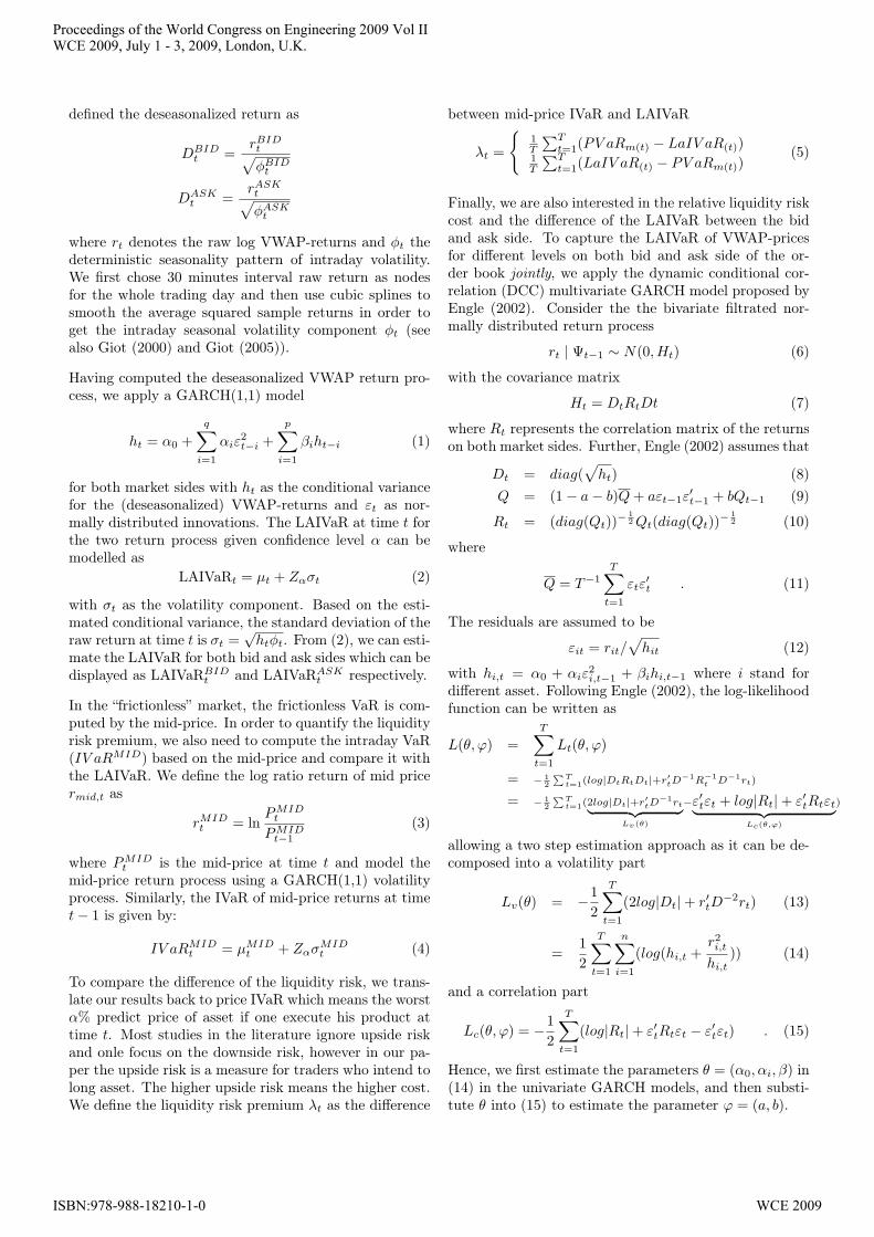
defined the deseasonalized return as

DBIDt =

rBIDt√φBID

t

DASKt =

rASKt√φASK

t

where rt denotes the raw log VWAP-returns and φt thedeterministic seasonality pattern of intraday volatility.We first chose 30 minutes interval raw return as nodesfor the whole trading day and then use cubic splines tosmooth the average squared sample returns in order toget the intraday seasonal volatility component φt (seealso Giot (2000) and Giot (2005)).

Having computed the deseasonalized VWAP return pro-cess, we apply a GARCH(1,1) model

ht = α0 +q∑

i=1

αiε2t−i +

p∑

i=1

βiht−i (1)

for both market sides with ht as the conditional variancefor the (deseasonalized) VWAP-returns and εt as nor-mally distributed innovations. The LAIVaR at time t forthe two return process given confidence level α can bemodelled as

LAIVaRt = µt + Zασt (2)

with σt as the volatility component. Based on the esti-mated conditional variance, the standard deviation of theraw return at time t is σt =

√htφt. From (2), we can esti-

mate the LAIVaR for both bid and ask sides which can bedisplayed as LAIVaRBID

t and LAIVaRASKt respectively.

In the “frictionless” market, the frictionless VaR is com-puted by the mid-price. In order to quantify the liquidityrisk premium, we also need to compute the intraday VaR(IV aRMID) based on the mid-price and compare it withthe LAIVaR. We define the log ratio return of mid pricermid,t as

rMIDt = ln

PMIDt

PMIDt−1

(3)

where PMIDt is the mid-price at time t and model the

mid-price return process using a GARCH(1,1) volatilityprocess. Similarly, the IVaR of mid-price returns at timet− 1 is given by:

IV aRMIDt = µMID

t + ZασMIDt (4)

To compare the difference of the liquidity risk, we trans-late our results back to price IVaR which means the worstα% predict price of asset if one execute his product attime t. Most studies in the literature ignore upside riskand onle focus on the downside risk, however in our pa-per the upside risk is a measure for traders who intend tolong asset. The higher upside risk means the higher cost.We define the liquidity risk premium λt as the difference

between mid-price IVaR and LAIVaR

λt =

{1T

∑Tt=1(PV aRm(t) − LaIV aR(t))

1T

∑Tt=1(LaIV aR(t) − PV aRm(t))

(5)

Finally, we are also interested in the relative liquidity riskcost and the difference of the LAIVaR between the bidand ask side. To capture the LAIVaR of VWAP-pricesfor different levels on both bid and ask side of the or-der book jointly, we apply the dynamic conditional cor-relation (DCC) multivariate GARCH model proposed byEngle (2002). Consider the the bivariate filtrated nor-mally distributed return process

rt | Ψt−1 ∼ N(0,Ht) (6)

with the covariance matrix

Ht = DtRtDt (7)

where Rt represents the correlation matrix of the returnson both market sides. Further, Engle (2002) assumes that

Dt = diag(√

ht) (8)Q = (1− a− b)Q + aεt−1ε

′t−1 + bQt−1 (9)

Rt = (diag(Qt))−12 Qt(diag(Qt))−

12 (10)

where

Q = T−1T∑

t=1

εtε′t . (11)

The residuals are assumed to be

εit = rit/√

hit (12)

with hi,t = α0 + αiε2i,t−1 + βihi,t−1 where i stand for

different asset. Following Engle (2002), the log-likelihoodfunction can be written as

L(θ, ϕ) =T∑

t=1

Lt(θ, ϕ)

= − 12

∑Tt=1(log|DtRtDt|+r′tD

−1R−1t D−1rt)

= − 12

∑Tt=1(2log|Dt|+r′tD

−1rt︸︷︷︸Lv(θ)

−ε′tεt + log|Rt|+ ε′tRtεt︸︷︷︸Lc(θ,ϕ)

)

allowing a two step estimation approach as it can be de-composed into a volatility part

Lv(θ) = −12

T∑t=1

(2log|Dt|+ r′tD−2rt) (13)

=12

T∑t=1

n∑

i=1

(log(hi,t +r2i,t

hi,t)) (14)

and a correlation part

Lc(θ, ϕ) = −12

T∑t=1

(log|Rt|+ ε′tRtεt − ε′tεt) . (15)

Hence, we first estimate the parameters θ = (α0, αi, β) in(14) in the univariate GARCH models, and then substi-tute θ into (15) to estimate the parameter ϕ = (a, b).


ISBN:978-988-18210-1-0 WCE 2009

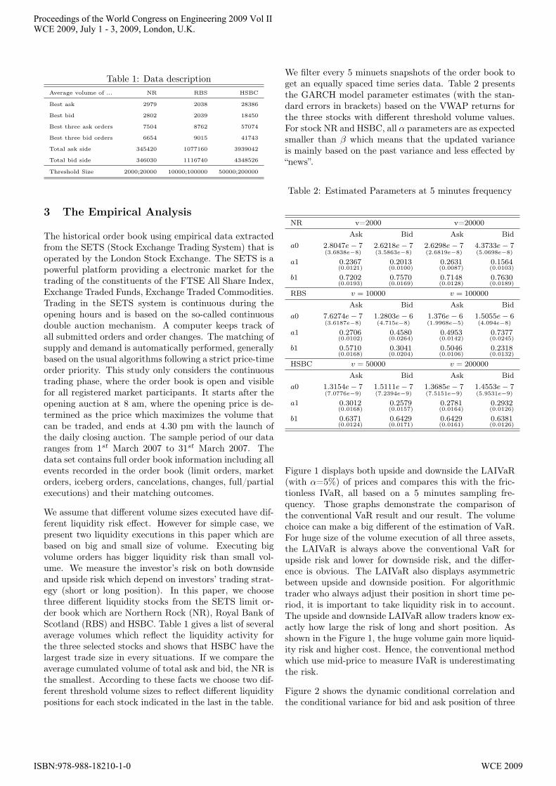
Table 1: Data descriptionAverage volume of ... NR RBS HSBC

Best ask 2979 2038 28386

Best bid 2802 2039 18450

Best three ask orders 7504 8762 57074

Best three bid orders 6654 9015 41743

Total ask side 345420 1077160 3939042

Total bid side 346030 1116740 4348526

Threshold Size 2000;20000 10000;100000 50000;200000

3 The Empirical Analysis

The historical order book using empirical data extractedfrom the SETS (Stock Exchange Trading System) that isoperated by the London Stock Exchange. The SETS is apowerful platform providing a electronic market for thetrading of the constituents of the FTSE All Share Index,Exchange Traded Funds, Exchange Traded Commodities.Trading in the SETS system is continuous during theopening hours and is based on the so-called continuousdouble auction mechanism. A computer keeps track ofall submitted orders and order changes. The matching ofsupply and demand is automatically performed, generallybased on the usual algorithms following a strict price-timeorder priority. This study only considers the continuoustrading phase, where the order book is open and visiblefor all registered market participants. It starts after theopening auction at 8 am, where the opening price is de-termined as the price which maximizes the volume thatcan be traded, and ends at 4.30 pm with the launch ofthe daily closing auction. The sample period of our dataranges from 1st March 2007 to 31st March 2007. Thedata set contains full order book information including allevents recorded in the order book (limit orders, marketorders, iceberg orders, cancelations, changes, full/partialexecutions) and their matching outcomes.

We assume that different volume sizes executed have dif-ferent liquidity risk effect. However for simple case, wepresent two liquidity executions in this paper which arebased on big and small size of volume. Executing bigvolume orders has bigger liquidity risk than small vol-ume. We measure the investor’s risk on both downsideand upside risk which depend on investors’ trading strat-egy (short or long position). In this paper, we choosethree different liquidity stocks from the SETS limit or-der book which are Northern Rock (NR), Royal Bank ofScotland (RBS) and HSBC. Table 1 gives a list of severalaverage volumes which reflect the liquidity activity forthe three selected stocks and shows that HSBC have thelargest trade size in every situations. If we compare theaverage cumulated volume of total ask and bid, the NR isthe smallest. According to these facts we choose two dif-ferent threshold volume sizes to reflect different liquiditypositions for each stock indicated in the last in the table.

We filter every 5 minuets snapshots of the order book toget an equally spaced time series data. Table 2 presentsthe GARCH model parameter estimates (with the stan-dard errors in brackets) based on the VWAP returns forthe three stocks with different threshold volume values.For stock NR and HSBC, all α parameters are as expectedsmaller than β which means that the updated varianceis mainly based on the past variance and less effected by“news”.

Table 2: Estimated Parameters at 5 minutes frequency

NR v=2000 v=20000Ask Bid Ask Bid

a0 2.8047e− 7(3.6838e−8)

2.6218e− 7(3.5863e−8)

2.6298e− 7(2.6819e−8)

4.3733e− 7(5.0698e−8)

a1 0.2367(0.0121)

0.2013(0.0100)

0.2631(0.0087)

0.1564(0.0103)

b1 0.7202(0.0193)

0.7570(0.0169)

0.7148(0.0128)

0.7630(0.0189)

RBS v = 10000 v = 100000

Ask Bid Ask Bida0 7.6274e− 7

(3.6187e−8)1.2803e− 6(4.715e−8)

1.376e− 6(1.9968e−5)

1.5055e− 6(4.094e−8)

a1 0.2706(0.0102)

0.4580(0.0264)

0.4953(0.0142)

0.7377(0.0245)

b1 0.5710(0.0168)

0.3041(0.0204)

0.5046(0.0106)

0.2318(0.0132)

HSBC v = 50000 v = 200000

Ask Bid Ask Bida0 1.3154e− 7

(7.0776e−9)1.5111e− 7(7.2394e−9)

1.3685e− 7(7.5151e−9)

1.4553e− 7(5.9531e−9)

a1 0.3012(0.0168)

0.2579(0.0157)

0.2781(0.0164)

0.2932(0.0126)

b1 0.6371(0.0124)

0.6429(0.0171)

0.6429(0.0161)

0.6381(0.0126)

Figure 1 displays both upside and downside the LAIVaR(with α=5%) of prices and compares this with the fric-tionless IVaR, all based on a 5 minutes sampling fre-quency. Those graphs demonstrate the comparison ofthe conventional VaR result and our result. The volumechoice can make a big different of the estimation of VaR.For huge size of the volume execution of all three assets,the LAIVaR is always above the conventional VaR forupside risk and lower for downside risk, and the differ-ence is obvious. The LAIVaR also displays asymmetricbetween upside and downside position. For algorithmictrader who always adjust their position in short time pe-riod, it is important to take liquidity risk in to account.The upside and downside LAIVaR allow traders know ex-actly how large the risk of long and short position. Asshown in the Figure 1, the huge volume gain more liquid-ity risk and higher cost. Hence, the conventional methodwhich use mid-price to measure IVaR is underestimatingthe risk.

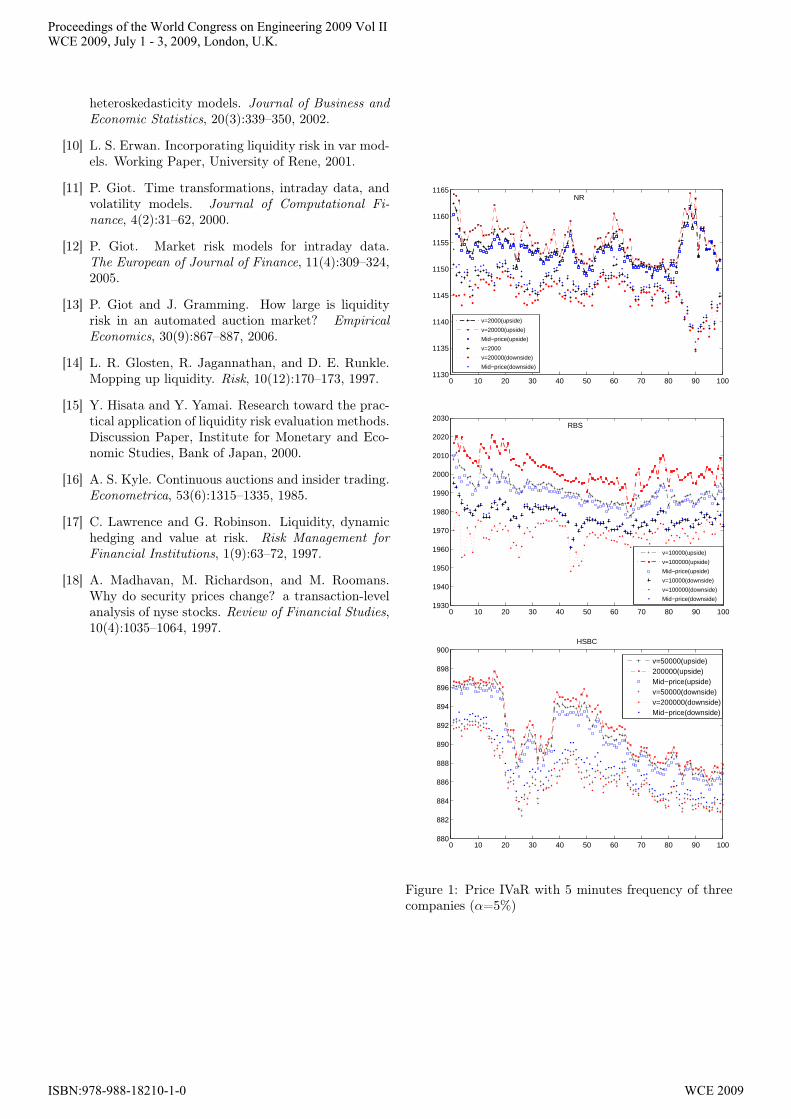
Figure 2 shows the dynamic conditional correlation andthe conditional variance for bid and ask position of three


ISBN:978-988-18210-1-0 WCE 2009

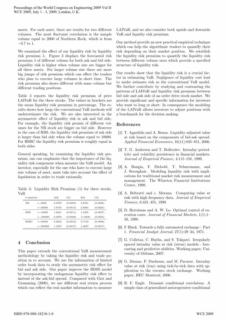
assets. For each asset, there are results for two differentvolumes. The most fluctuant correlation is the samplevolume equal to 2000 of Northern Rock, which is from−0.7 to 1.

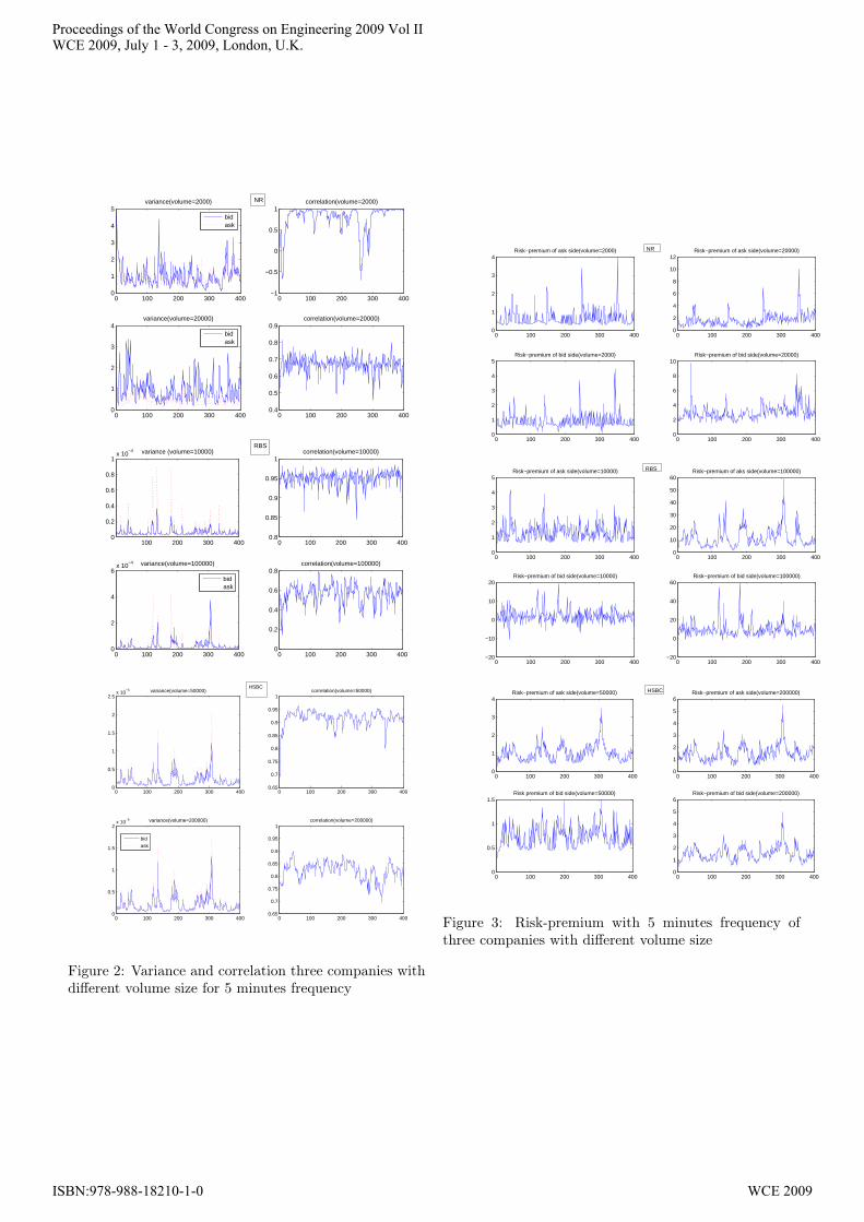
We examined the effect of our liquidity risk by liquidityrisk premium λ. Figure 3 displays the forecasted riskpremium λ of different volume for both ask and bid side.Liquidity risk is higher when volume size are bigger forall three assets. For larger volume size there are morebig jumps of risk premium which can effect the traderswho plan to execute large volumes in short time. Therisk premium also shows different with same volume butdifferent trading positions.

Table 3 reports the liquidity risk premium of priceLAIVaR for the three stocks. The values in brackets arethe mean liquidity risk premium in percentage. The re-sults shows how large the conventional VaR methods willunderestimate the risk. We are also interested in theasymmetric effect of liquidity risk in ask and bid side.For example, the liquidity risk premia of different vol-umes for the NR stock are bigger on bid side. Howeverin the case of RBS, the liquidity risk premium of ask sideis larger than bid side when the volume equal to 10000.For HSBC the liquidity risk premium is roughly equal inboth sides.

General speaking, by examining the liquidity risk pre-mium, one can emphasize that the importance of the liq-uidity risk component when measure the VaR model. Aninvestor, especially for the one who have to execute largesize volume of asset, must take into account the effect ofliquidation in order to trade rationally.

Table 3: Liquidity Risk Premium (λ) for three stocks.VaR

5 minutes Ask (%) Bid (%)

NR v=2000 0.3370 (0.0005) 0.8781 (0.0008)

v=20000 1.6755 (0.0014) 2.9364 (0.0025)

RBS v=10000 1.9241 (0.0011) 1.3305 (0.0007)

v=100000 9.4878 (0.0048) 11.9636 (0.0054)

HSBC v=50000 0.9624 (0.0010) 0.7133 (0.0008)

v=200000 1.4567 (0.0017) 1.4827 (0.0017)

4 Conclusion

This paper extends the conventional VaR measurementmethodology by taking the liquidity risk and trade po-sition in to account. We use the information of limitedorder book data to study the asymmetric risk effect forbid and ask side. Our paper improve the BDSS modelby incorporating the endogenous liquidity risk effect toinstead of the ask-bid spread. Compared with Giot andGramming (2006), we use different real return processwhich can reflect the real market information to measure

LAIVaR, and we also consider both upside and downsideVaR and liquidty risk premium.

Our method provide an new practical empirical techniquewhich can help the algorithmic traders to quantify theirrisk depending on their market position. We establishthe liquidity risk premium to quantify the liquidity riskbetween different volume sizes which provide a specifiedstructure of liquidity risk.

Our results show that the liquidity risk is a crucial fac-tor in estimating VaR. Negligence of liquidity cost leadto under estimate risk as the conventional VaR model.We further contribute by studying and contrasting thepatterns of LAIVaR and liquidity risk premium betweenbid side and ask side of an order drive stock market. Weprovide significant and specific information for investorswho want to long or short. In consequence the modelingof the LAIVaR allows investors to adjust positions witha benchmark for the decision making.

References

[1] T. Agnelidis and A. Benos. Liquidity adjusted valueat risk based on the components of bid-ask spread.Applied Financial Economics, 16(11):835–851, 2006.

[2] T. G. Andersen and T. Bollerslev. Intraday period-icity and volatility persistence in financial markets.Journal of Empirical Finance, 4:115–158, 1999.

[3] A. Bangia, F. Diebold, T. Schuermann, andJ. Stroughair. Modeling liquidity risk with impli-cations for traditional market risk measurement andmanagement. The Wharton Financial InstitutionsCenter, 1999.

[4] A. Beltratti and c. Morana. Computing value atrisk with high frequency data. Journal of EmpiricalFinance, 6:431–455, 1999.

[5] D. Bertsimas and A. W. Lo. Optimal control of ex-ecution costs. Journal of Financial Markets, 1(1):1–50, 1998.

[6] F Black. Towards a fully automated exchange : Part1. Financial Analyst Journal, 27(1):29–34, 1971.

[7] G. Colletaz, C. Hurlin, and S. Tokpavi. Irregularlyspaced intraday value at risk (isivar) models - fore-casting and predictive abilities. Working paper, Uni-versity of Orléans, 2007.

[8] G. Dionne, P. Duchesne, and M. Pacurar. Intradayvalue at risk (ivar) using tick-by-tick data with ap-plication to the toronto stock exchange. Workingpaper, HEC Montreal, 2006.

[9] R. F. Engle. Dynamic conditional correlation: Asimple class of generalized autoregressive conditional


ISBN:978-988-18210-1-0 WCE 2009

heteroskedasticity models. Journal of Business andEconomic Statistics, 20(3):339–350, 2002.

[10] L. S. Erwan. Incorporating liquidity risk in var mod-els. Working Paper, University of Rene, 2001.

[11] P. Giot. Time transformations, intraday data, andvolatility models. Journal of Computational Fi-nance, 4(2):31–62, 2000.

[12] P. Giot. Market risk models for intraday data.The European of Journal of Finance, 11(4):309–324,2005.

[13] P. Giot and J. Gramming. How large is liquidityrisk in an automated auction market? EmpiricalEconomics, 30(9):867–887, 2006.

[14] L. R. Glosten, R. Jagannathan, and D. E. Runkle.Mopping up liquidity. Risk, 10(12):170–173, 1997.

[15] Y. Hisata and Y. Yamai. Research toward the prac-tical application of liquidity risk evaluation methods.Discussion Paper, Institute for Monetary and Eco-nomic Studies, Bank of Japan, 2000.

[16] A. S. Kyle. Continuous auctions and insider trading.Econometrica, 53(6):1315–1335, 1985.

[17] C. Lawrence and G. Robinson. Liquidity, dynamichedging and value at risk. Risk Management forFinancial Institutions, 1(9):63–72, 1997.

[18] A. Madhavan, M. Richardson, and M. Roomans.Why do security prices change? a transaction-levelanalysis of nyse stocks. Review of Financial Studies,10(4):1035–1064, 1997.

0 10 20 30 40 50 60 70 80 90 1001130

1135

1140

1145

1150

1155

1160

1165NR

v=2000(upside)

v=20000(upside)

Mid−price(upside)

v=2000

v=20000(downside)

Mid−price(downside)

0 10 20 30 40 50 60 70 80 90 1001930

1940

1950

1960

1970

1980

1990

2000

2010

2020

2030RBS

v=10000(upside)

v=100000(upside)

Mid−price(upside)

v=10000(downside)

v=100000(downside)

Mid−price(downside)

0 10 20 30 40 50 60 70 80 90 100880

882

884

886

888

890

892

894

896

898

900HSBC

v=50000(upside)200000(upside)Mid−price(upside)v=50000(downside)v=200000(downside)Mid−price(downside)

Figure 1: Price IVaR with 5 minutes frequency of threecompanies (α=5%)


ISBN:978-988-18210-1-0 WCE 2009

0 100 200 300 4000

1

2

3

4

5variance(volume=2000)

0 100 200 300 400−1

−0.5

0

0.5

1correlation(volume=2000)

0 100 200 300 4000

1

2

3

4variance(volume=20000)

0 100 200 300 4000.4

0.5

0.6

0.7

0.8

0.9correlation(volume=20000)

bidask

bidask

NR

100 200 300 4000

0.2

0.4

0.6

0.8

1x 10

−4 variance (volume=10000)

0 100 200 300 4000.8

0.85

0.9

0.95


0 100 200 300 4000

2

4

6x 10

−4 variance(volume=100000)

0 100 200 300 4000

0.2

0.4

0.6

0.8correlation(volume=100000)

bidask

RBS

0 100 200 300 4000

0.5

1

1.5

2x 10


0 100 200 300 4000.65

0.7

0.75

0.8

0.85

0.9

0.95


bidask

0 100 200 300 4000

0.5

1

1.5

2

2.5x 10


0 100 200 300 4000.65

0.7

0.75

0.8

0.85

0.9

0.95


HSBC

Figure 2: Variance and correlation three companies withdifferent volume size for 5 minutes frequency

0 100 200 300 4000

1

2

3

4Risk−premium of ask side(volume=2000)

0 100 200 300 4000

2

4

6

8

10


0 100 200 300 4000

1

2

3

4

5Risk−premium of bid side(volume=2000)

0 100 200 300 4000

2

4

6

8


NR

0 100 200 300 400−20

−10

0

10


0 100 200 300 400−20

0

20

40


0 100 200 300 4000

1

2

3

4


0 100 200 300 4000

10

20

30

40

50

60Risk−premium of aks side(volume=100000)RBS

0 100 200 300 4000

1

2

3


0 100 200 300 4000

1

2

3

4

5


0 100 200 300 4000

0.5

1

1.5Risk premium of bid side(volume=50000)

0 100 200 300 4000

1

2

3

4

5


HSBC

Figure 3: Risk-premium with 5 minutes frequency ofthree companies with different volume size


ISBN:978-988-18210-1-0 WCE 2009

Documents

LiquidityAdjustedIntradayValueatRisk - iaeng.org · pt `ASK t wherert denotestherawlogVWAP-returnsand`t the deterministic seasonality pattern of intraday volatility. We ﬁrst chose