Liquidity Ratiostalentbucket.weebly.com/.../andrews_corporation.docx · Web viewThis would require increasing capacity, spending money on marketing, etc. (all of which would lower

Running head: ANDREWS CORPORATION

Andrews Corporation

by

Glen Sallee

Business Seminar BUS 496 Professor Daniel Morgan 05/25/2014

ANDREWS CORPORATION

Abstract

The purpose of the paper is to explain and illustrate the effectiveness of the various financial

tools employed by Team Andrews during the Capstone simulation. Andrews employed trend

analysis, where we plotted selected ratios over time to show whether our condition was

improving or deteriorating. In addition to that, we benchmarked our results against the average

of the six best firms in the sensor industry.

ii

ANDREWS CORPORATION

For the students of the University of La Verne’s Business Seminar

and Strategy class, and every other class I had the opportunity to

take at this wonderful school, thank you for teaching me so much.

iii

ANDREWS CORPORATION

CONTENTS

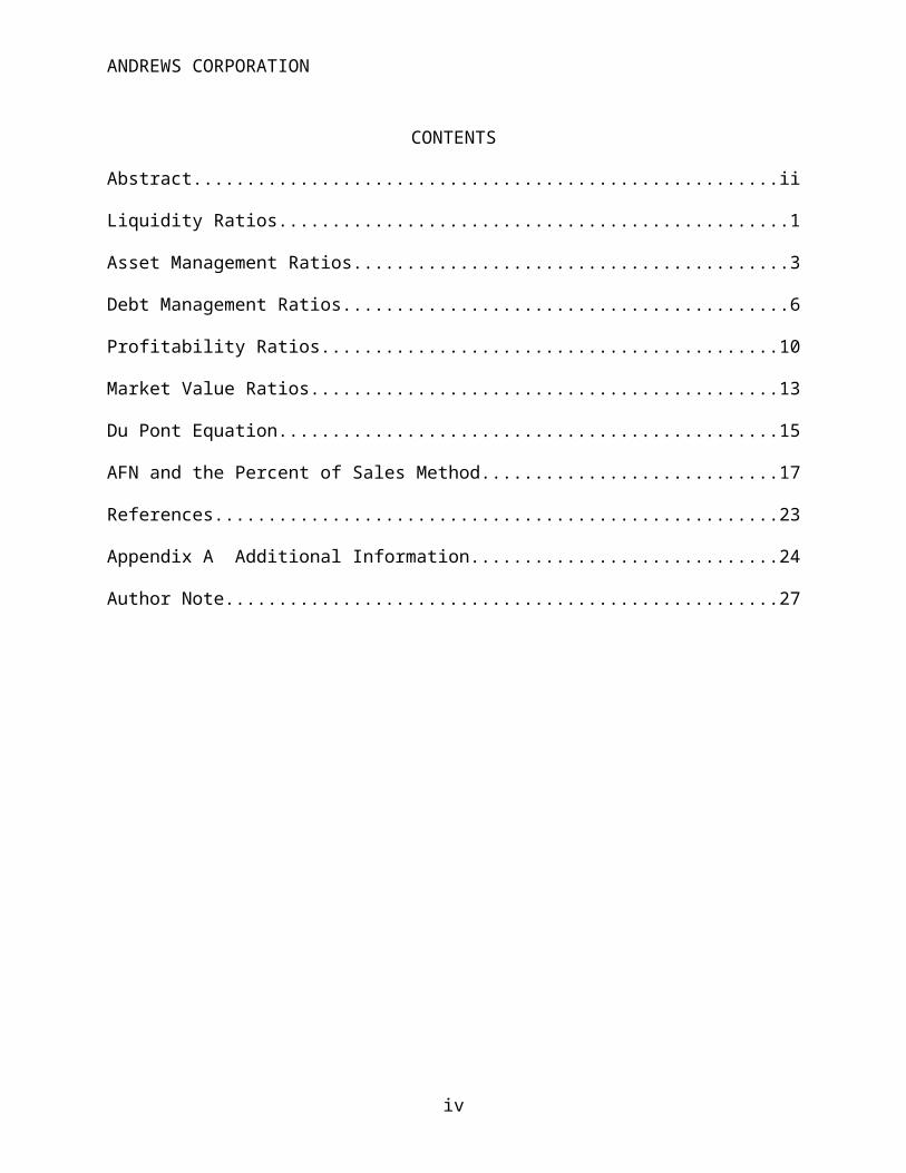
Abstract............................................................................................................................................ii

Liquidity Ratios...............................................................................................................................1

Asset Management Ratios................................................................................................................3

Debt Management Ratios.................................................................................................................6

Profitability Ratios.........................................................................................................................10

Market Value Ratios......................................................................................................................13

Du Pont Equation...........................................................................................................................15

AFN and the Percent of Sales Method...........................................................................................17

References......................................................................................................................................23

Appendix A Additional Information.............................................................................................24

Author Note...................................................................................................................................27

iv

ANDREWS CORPORATION

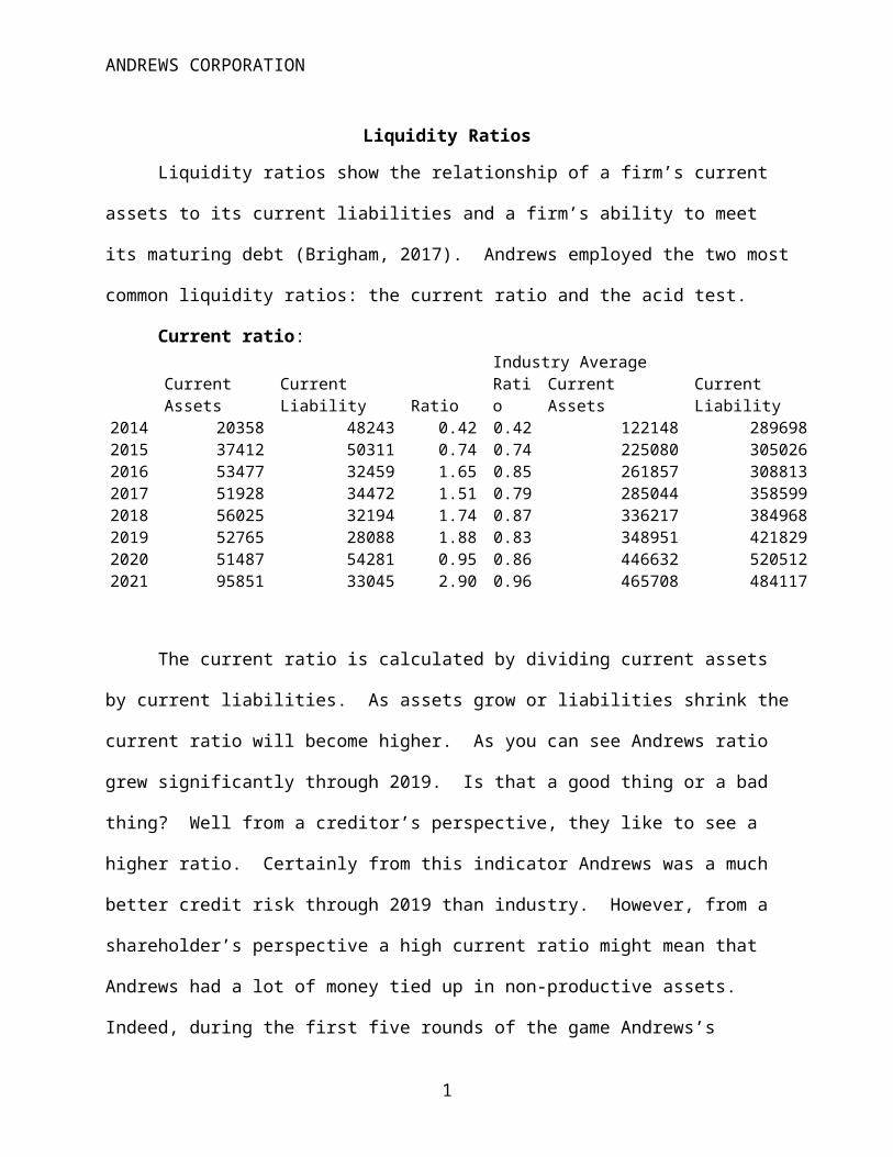
Liquidity Ratios

Liquidity ratios show the relationship of a firm’s current assets to its current liabilities

and a firm’s ability to meet its maturing debt (Brigham, 2017). Andrews employed the two most

common liquidity ratios: the current ratio and the acid test.

Current ratio:Industry Average

Current Assets Current Liability Ratio Ratio Current Assets Current Liability2014 20358 48243 0.42 0.42 122148 2896982015 37412 50311 0.74 0.74 225080 3050262016 53477 32459 1.65 0.85 261857 3088132017 51928 34472 1.51 0.79 285044 3585992018 56025 32194 1.74 0.87 336217 3849682019 52765 28088 1.88 0.83 348951 4218292020 51487 54281 0.95 0.86 446632 5205122021 95851 33045 2.90 0.96 465708 484117

The current ratio is calculated by dividing current assets by current liabilities. As assets

grow or liabilities shrink the current ratio will become higher. As you can see Andrews ratio

grew significantly through 2019. Is that a good thing or a bad thing? Well from a creditor’s

perspective, they like to see a higher ratio. Certainly from this indicator Andrews was a much

better credit risk through 2019 than industry. However, from a shareholder’s perspective a high

current ratio might mean that Andrews had a lot of money tied up in non-productive assets.

Indeed, during the first five rounds of the game Andrews’s strategy was to pay down liabilities

and retain as much cash as possible to hedge against any “Big Al” emergency loans. We decided

to stop offering equity as a means of holding of Big Al at bay, pay a dividend of 2.5% to release

some cash, stop making extra debt payments, and taking on long term debt to cover financing

needs. We were successfully able to lower our current ratio to a level more in line with industry.

1

ANDREWS CORPORATION 2

The Acid Test:Industry Average

Current Assets

Inventory

Current Liability Ratio

Ratio Current Assets

Inventory

Current Liability

2014 20358 8617 48243 0.24 0.24 122148 $51,702 2896982015 37412 6726 50311 0.61 0.61 225080 $39,962 3050262016 53477 926 32459 1.62 0.66 261857 $57,862 3088132017 51928 551 34472 1.49 0.48 285044 $113,219 3585992018 56025 6736 32194 1.53 0.73 336217 54464 3849682019 52765 2485 28088 1.79 0.68 348951 63012 4218292020 51487 7864 54281 0.80 0.70 446632 83620 5205122021 95851 5444 33045 2.74 0.82 465708 69798 484117

The acid test is calculated by deducting inventories from the current assets and then

dividing the remainder by current liabilities. Inventories are the least liquid of a firm’s current

assets and inventories are the most likely current asset to suffer a loss in a bankruptcy (Brigham,

2017). This is the reason that the capstone game penalized a firm if they had more than two

months inventory at the end of each round. Ratios below one indicate that inventories would

have to be liquidated to pay off current liabilities should the need arise. For most of the game,

Andrews’s ratio has been better than industry. In 2020, Andrews reported its highest inventory

level and saw its current assets shrink resulting in a ratio below one. By the close of the

simulation, this ratio improved dramatically.


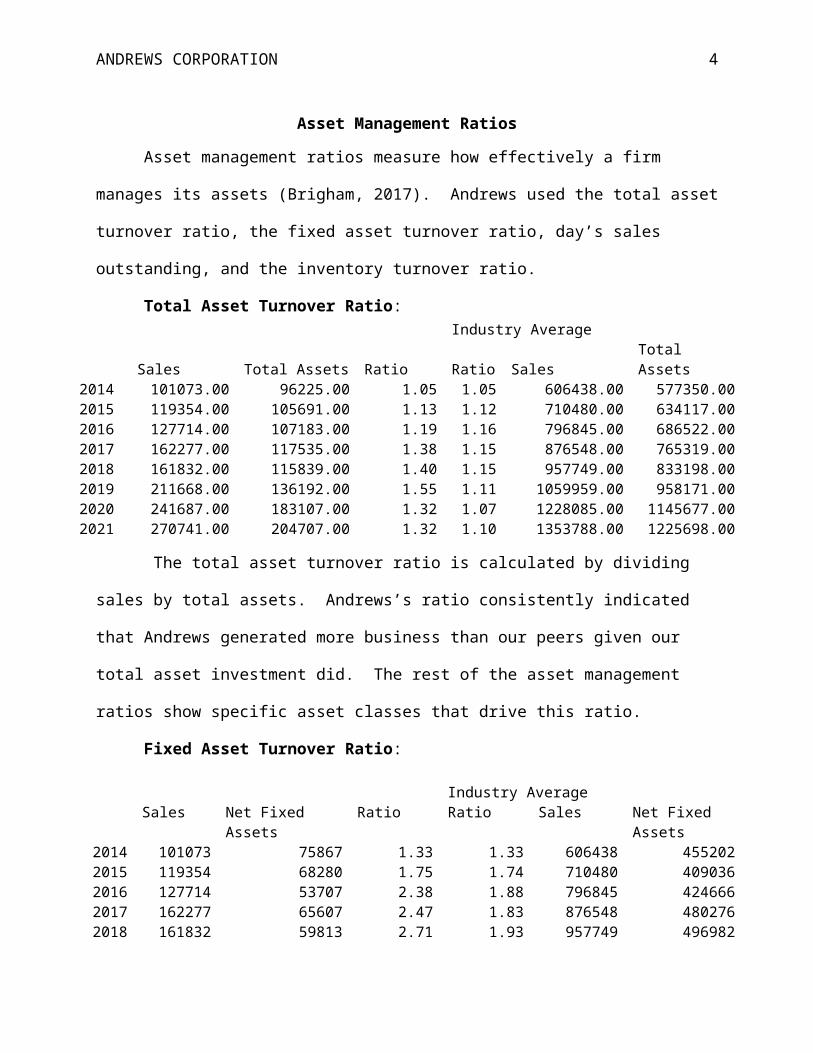
Asset Management Ratios

Asset management ratios measure how effectively a firm manages its assets (Brigham,

2017). Andrews used the total asset turnover ratio, the fixed asset turnover ratio, day’s sales

outstanding, and the inventory turnover ratio.

Total Asset Turnover Ratio:Industry Average

Sales Total Assets Ratio Ratio Sales Total Assets2014 101073.00 96225.00 1.05 1.05 606438.00 577350.002015 119354.00 105691.00 1.13 1.12 710480.00 634117.002016 127714.00 107183.00 1.19 1.16 796845.00 686522.002017 162277.00 117535.00 1.38 1.15 876548.00 765319.002018 161832.00 115839.00 1.40 1.15 957749.00 833198.002019 211668.00 136192.00 1.55 1.11 1059959.00 958171.002020 241687.00 183107.00 1.32 1.07 1228085.00 1145677.002021 270741.00 204707.00 1.32 1.10 1353788.00 1225698.00

The total asset turnover ratio is calculated by dividing sales by total assets. Andrews’s

ratio consistently indicated that Andrews generated more business than our peers given our total

asset investment did. The rest of the asset management ratios show specific asset classes that

drive this ratio.

Fixed Asset Turnover Ratio:

Industry AverageSales Net Fixed Assets Ratio Ratio Sales Net Fixed Assets

2014 101073 75867 1.33 1.33 606438 4552022015 119354 68280 1.75 1.74 710480 4090362016 127714 53707 2.38 1.88 796845 4246662017 162277 65607 2.47 1.83 876548 4802762018 161832 59813 2.71 1.93 957749 4969822019 211668 83427 2.54 1.74 1059959 6092192020 241687 131621 1.84 1.76 1228085 6990472021 270741 108857 2.49 1.78 1353788 759992


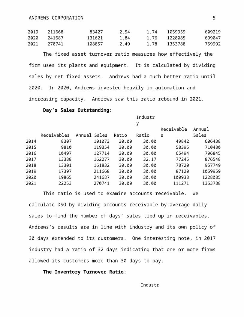
The fixed asset turnover ratio measures how effectively the firm uses its plants and

equipment. It is calculated by dividing sales by net fixed assets. Andrews had a much better

ratio until 2020. In 2020, Andrews invested heavily in automation and increasing capacity.

Andrews saw this ratio rebound in 2021.

Day’s Sales Outstanding:Industry

Receivables Annual Sales Ratio Ratio Receivables Annual Sales2014 8307 101073 30.00 30.00 49842 6064382015 9810 119354 30.00 30.00 58395 7104802016 10497 127714 30.00 30.00 65494 7968452017 13338 162277 30.00 32.17 77245 8765482018 13301 161832 30.00 30.00 78720 9577492019 17397 211668 30.00 30.00 87120 10599592020 19865 241687 30.00 30.00 100938 12280852021 22253 270741 30.00 30.00 111271 1353788

This ratio is used to examine accounts receivable. We calculate DSO by dividing

accounts receivable by average daily sales to find the number of days’ sales tied up in

receivables. Andrews’s results are in line with industry and its own policy of 30 days extended

to its customers. One interesting note, in 2017 industry had a ratio of 32 days indicating that one

or more firms allowed its customers more than 30 days to pay.

The Inventory Turnover Ratio:

IndustryContribution Inventories Ratio Ratio Contribution Inventories

2014 80100 8617 9.30 9.30 480600 517022015 86526 6726 12.86 13.20 527512 399622016 93638 925 101.23 10.25 593055 578622017 125094 551 227.03 6.04 683961 1132192018 125902 6736 18.69 13.19 718375 544642019 145736 2485 58.65 12.18 767485 630122020 162613 7864 20.68 10.44 873164 836202021 137847 5444 25.32 10.92 762305 69798


This ratio is calculated by dividing costs of goods sold (COGS) except depreciation by

inventories. COGS are used rather than sales as sales include costs and profits while inventories

are generally reported at cost only (Brigham, 2017). Andrews typically had much lower

inventory levels than did industry resulting in a much higher historical ratio. However, this did

not always indicate good news for Andrews as in several years Andrews stocked out of sensors.

In the case of stock outs, Andrews missed potential sales.


Debt Management Ratios

Financial leverage is defined as the extent that a firm uses debt financing. “This is

important for three reasons: (1) Stockholders can control a firm with smaller investments of their

own equity if they finance part of the firm with debt. (2) If the firm’s assets generate a higher

pre-tax return than the interest rate on debt, then shareholder’s returns are magnified. Of course,

shareholder losses are also magnified if assets generate a pre-tax return less than the interest rate.

(3) If a firm has high leverage, even a small decline in performance might cause the firm’s value

to fall below the amount it owes creditors” (Brigham, 2017). Andrews used the debt to asset,

debt to equity, market debt ratio, liabilities to assets, times interest earned ratio, and the EBITDA

coverage ratio.

Debt to Asset Ratio:

Industry AverageDebt Assets Ratio Ratio Debt Assets

2014 41700 96225 0.43 0.43 250200 5773502015 46133 105691 0.44 0.42 265365 6341172016 28020 107183 0.26 0.39 265113 6865222017 28020 117535 0.24 0.40 307956 7653192018 20850 115839 0.18 0.26 214066 8331982019 20850 136192 0.15 0.27 259668 9581712020 25000 183107 0.14 0.22 256764 11456772021 25000 204707 0.12 0.23 283686 1225698

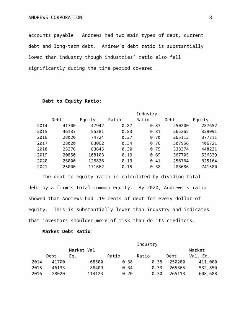
To calculate the debt to asset ratio we divide total debt by total assets. We do not

include other liabilities like accounts payable. Andrews had two main types of debt, current debt

and long-term debt. Andrew’s debt ratio is substantially lower than industry though industries’

ratio also fell significantly during the time period covered.


Debt to Equity Ratio:

IndustryDebt Equity Ratio Ratio Debt Equity

2014 41700 47942 0.87 0.87 250200 2876522015 46133 55381 0.83 0.81 265365 3290912016 28020 74724 0.37 0.70 265113 3777112017 28020 83062 0.34 0.76 307956 4067212018 25376 83645 0.30 0.75 338374 4482312019 20850 108103 0.19 0.69 367705 5363392020 25000 128826 0.19 0.41 256764 6251642021 25000 171662 0.15 0.38 283686 741580

The debt to equity ratio is calculated by dividing total debt by a firm’s total common

equity. By 2020, Andrews’s ratio showed that Andrews had .19 cents of debt for every dollar of

equity. This is substantially lower than industry and indicates that investors shoulder more of

risk than do its creditors.

Market Debt Ratio:

IndustryDebt Market Val Eq. Ratio Ratio Debt Market Val. Eq.

2014 41700 68500 0.38 0.38 250200 411,0002015 46133 88409 0.34 0.33 265365 532,8502016 28020 114123 0.20 0.30 265113 608,6882017 28020 124051 0.18 0.35 307956 560,0262018 25376 111186 0.19 0.36 338374 602,0442019 20850 170141 0.11 0.33 367705 752,0792020 25000 252221 0.09 0.21 256764 987,2222021 25000 400496 0.06 0.17 283686 1,348,523

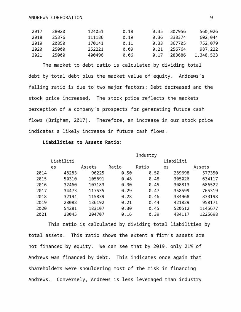
The market to debt ratio is calculated by dividing total debt by total debt plus the market

value of equity. Andrews’s falling ratio is due to two major factors: Debt decreased and the

stock price increased. The stock price reflects the markets perception of a company’s prospects

for generating future cash flows (Brigham, 2017). Therefore, an increase in our stock price

indicates a likely increase in future cash flows.


Liabilities to Assets Ratio:

IndustryLiabilities Assets Ratio Ratio Liabilities Assets

2014 48283 96225 0.50 0.50 289698 5773502015 50310 105691 0.48 0.48 305026 6341172016 32460 107183 0.30 0.45 308813 6865222017 34473 117535 0.29 0.47 358599 7653192018 32194 115839 0.28 0.46 384968 8331982019 28088 136192 0.21 0.44 421829 9581712020 54281 183107 0.30 0.45 520512 11456772021 33045 204707 0.16 0.39 484117 1225698

This ratio is calculated by dividing total liabilities by total assets. This ratio shows the

extent a firm’s assets are not financed by equity. We can see that by 2019, only 21% of Andrews

was financed by debt. This indicates once again that shareholders were shouldering most of the

risk in financing Andrews. Conversely, Andrews is less leveraged than industry.

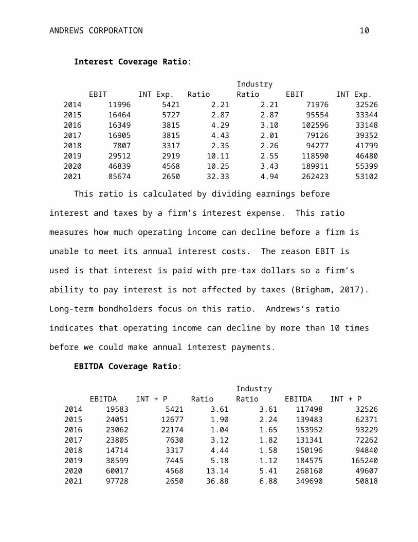
Interest Coverage Ratio:

IndustryEBIT INT Exp. Ratio Ratio EBIT INT Exp.

2014 11996 5421 2.21 2.21 71976 325262015 16464 5727 2.87 2.87 95554 333442016 16349 3815 4.29 3.10 102596 331482017 16905 3815 4.43 2.01 79126 393522018 7807 3317 2.35 2.26 94277 417992019 29512 2919 10.11 2.55 118590 464802020 46839 4568 10.25 3.43 189911 553992021 85674 2650 32.33 4.94 262423 53102

This ratio is calculated by dividing earnings before interest and taxes by a firm’s interest

expense. This ratio measures how much operating income can decline before a firm is unable to

meet its annual interest costs. The reason EBIT is used is that interest is paid with pre-tax dollars

so a firm’s ability to pay interest is not affected by taxes (Brigham, 2017). Long-term


bondholders focus on this ratio. Andrews’s ratio indicates that operating income can decline by

more than 10 times before we could make annual interest payments.

EBITDA Coverage Ratio:

IndustryEBITDA INT + P Ratio Ratio EBITDA INT + P

2014 19583 5421 3.61 3.61 117498 325262015 24051 12677 1.90 2.24 139483 623712016 23062 22174 1.04 1.65 153952 932292017 23805 7630 3.12 1.82 131341 722622018 14714 3317 4.44 1.58 150196 948402019 38599 7445 5.18 1.12 184575 1652402020 60017 4568 13.14 5.41 268160 496072021 97728 2650 36.88 6.88 349690 50818

In contrast to the interest coverage ratio, the EBITDA coverage ratio is used by banks

and short-term lenders whose typical loans are 5 years or less. The reason bankers use the

EBITDA coverage ratio rather than the ICR is that in the short-term depreciation generated funds

can be used to service debt. In the long-term, depreciation generated funds must be reinvested in

order to maintain plants and equipment (Brigham, 2017). Andrews’s covered its financial

charges 36.88 times in 2021, which is well above industry average.


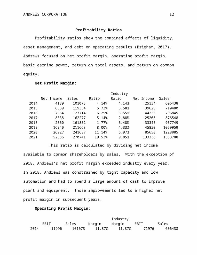
Profitability Ratios

Profitability ratios show the combined effects of liquidity, asset management, and debt on

operating results (Brigham, 2017). Andrews focused on net profit margin, operating profit

margin, basic earning power, return on total assets, and return on common equity.

Net Profit Margin:

IndustryNet Income Sales Ratio Ratio Net Income Sales

2014 4189 101073 4.14% 4.14% 25134 6064382015 6839 119354 5.73% 5.58% 39628 7104802016 7984 127714 6.25% 5.55% 44238 7968452017 8338 162277 5.14% 2.88% 25206 8765482018 2860 161832 1.77% 3.48% 33343 9577492019 16940 211668 8.00% 4.33% 45850 10599592020 26927 241687 11.14% 6.97% 85650 12280852021 52886 270741 19.53% 9.85% 133336 1353788

This ratio is calculated by dividing net income available to common shareholders

by sales. With the exception of 2018, Andrews’s net profit margin exceeded industry every year.

In 2018, Andrews was constrained by tight capacity and low automation and had to spend a large

amount of cash to improve plant and equipment. Those improvements led to a higher net profit

margin in subsequent years.

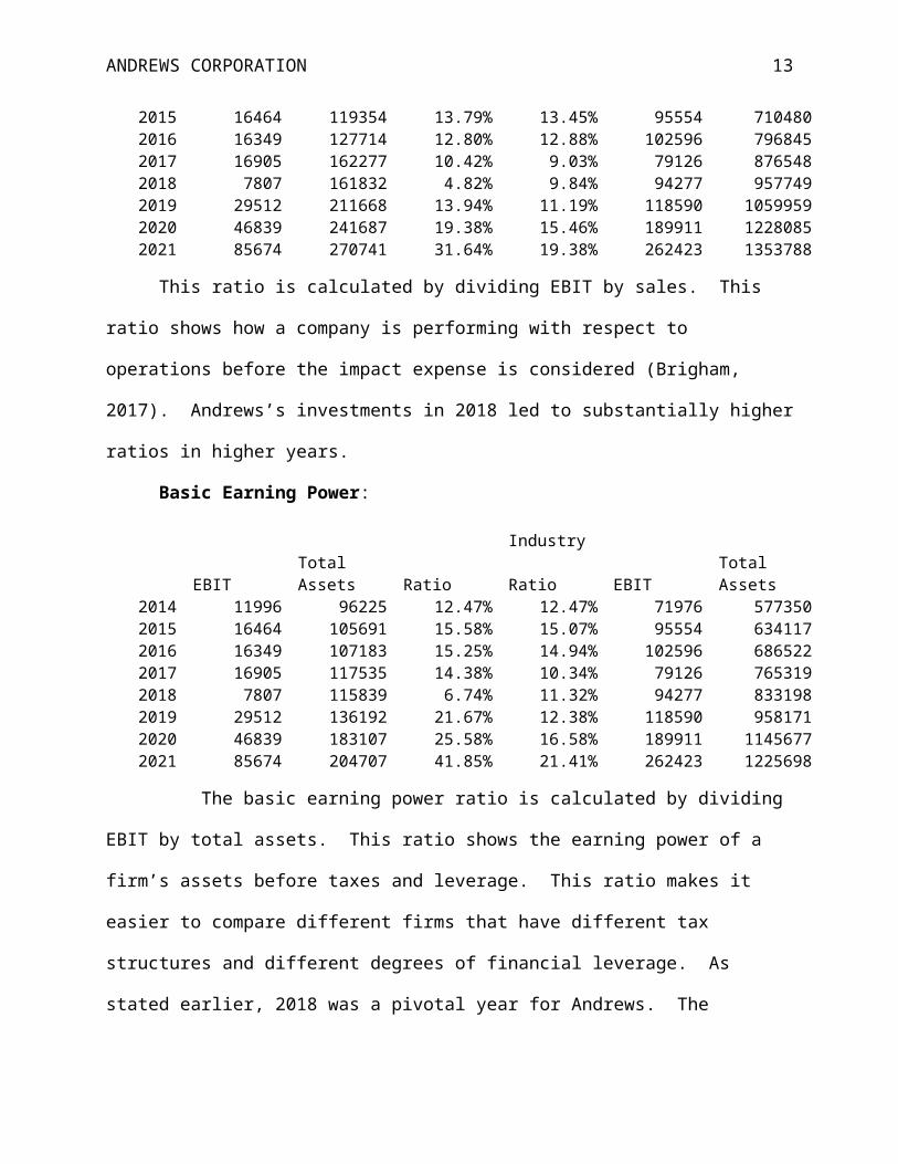
Operating Profit Margin:

IndustryEBIT Sales Margin Margin EBIT Sales

2014 11996 101073 11.87% 11.87% 71976 6064382015 16464 119354 13.79% 13.45% 95554 7104802016 16349 127714 12.80% 12.88% 102596 7968452017 16905 162277 10.42% 9.03% 79126 8765482018 7807 161832 4.82% 9.84% 94277 9577492019 29512 211668 13.94% 11.19% 118590 10599592020 46839 241687 19.38% 15.46% 189911 12280852021 85674 270741 31.64% 19.38% 262423 1353788


This ratio is calculated by dividing EBIT by sales. This ratio shows how a company is

performing with respect to operations before the impact expense is considered (Brigham, 2017).

Andrews’s investments in 2018 led to substantially higher ratios in higher years.

Basic Earning Power:

IndustryEBIT Total Assets Ratio Ratio EBIT Total Assets

2014 11996 96225 12.47% 12.47% 71976 5773502015 16464 105691 15.58% 15.07% 95554 6341172016 16349 107183 15.25% 14.94% 102596 6865222017 16905 117535 14.38% 10.34% 79126 7653192018 7807 115839 6.74% 11.32% 94277 8331982019 29512 136192 21.67% 12.38% 118590 9581712020 46839 183107 25.58% 16.58% 189911 11456772021 85674 204707 41.85% 21.41% 262423 1225698

The basic earning power ratio is calculated by dividing EBIT by total assets. This ratio

shows the earning power of a firm’s assets before taxes and leverage. This ratio makes it easier

to compare different firms that have different tax structures and different degrees of financial

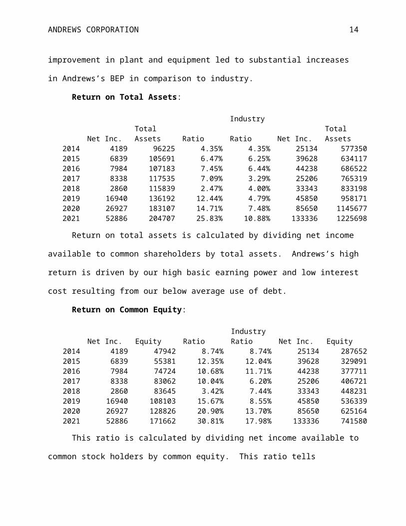
leverage. As stated earlier, 2018 was a pivotal year for Andrews. The improvement in plant and

equipment led to substantial increases in Andrews’s BEP in comparison to industry.

Return on Total Assets:

IndustryNet Inc. Total Assets Ratio Ratio Net Inc. Total Assets

2014 4189 96225 4.35% 4.35% 25134 5773502015 6839 105691 6.47% 6.25% 39628 6341172016 7984 107183 7.45% 6.44% 44238 6865222017 8338 117535 7.09% 3.29% 25206 7653192018 2860 115839 2.47% 4.00% 33343 8331982019 16940 136192 12.44% 4.79% 45850 9581712020 26927 183107 14.71% 7.48% 85650 11456772021 52886 204707 25.83% 10.88% 133336 1225698


Return on total assets is calculated by dividing net income available to common

shareholders by total assets. Andrews’s high return is driven by our high basic earning power

and low interest cost resulting from our below average use of debt.

Return on Common Equity:

IndustryNet Inc. Equity Ratio Ratio Net Inc. Equity

2014 4189 47942 8.74% 8.74% 25134 2876522015 6839 55381 12.35% 12.04% 39628 3290912016 7984 74724 10.68% 11.71% 44238 3777112017 8338 83062 10.04% 6.20% 25206 4067212018 2860 83645 3.42% 7.44% 33343 4482312019 16940 108103 15.67% 8.55% 45850 5363392020 26927 128826 20.90% 13.70% 85650 6251642021 52886 171662 30.81% 17.98% 133336 741580

This ratio is calculated by dividing net income available to common stock holders by

common equity. This ratio tells shareholders how their investment is doing. The ROE for

Andrews has made substantial improvements over industry.


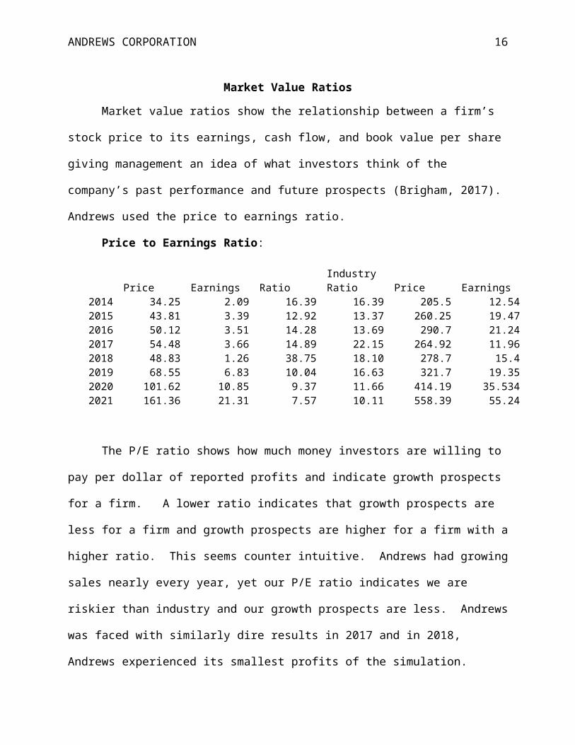
Market Value Ratios

Market value ratios show the relationship between a firm’s stock price to its earnings,

cash flow, and book value per share giving management an idea of what investors think of the

company’s past performance and future prospects (Brigham, 2017). Andrews used the price to

earnings ratio.

Price to Earnings Ratio:

IndustryPrice Earnings Ratio Ratio Price Earnings

2014 34.25 2.09 16.39 16.39 205.5 12.542015 43.81 3.39 12.92 13.37 260.25 19.472016 50.12 3.51 14.28 13.69 290.7 21.242017 54.48 3.66 14.89 22.15 264.92 11.962018 48.83 1.26 38.75 18.10 278.7 15.42019 68.55 6.83 10.04 16.63 321.7 19.352020 101.62 10.85 9.37 11.66 414.19 35.5342021 161.36 21.31 7.57 10.11 558.39 55.24

The P/E ratio shows how much money investors are willing to pay per dollar of reported

profits and indicate growth prospects for a firm. A lower ratio indicates that growth prospects

are less for a firm and growth prospects are higher for a firm with a higher ratio. This seems

counter intuitive. Andrews had growing sales nearly every year, yet our P/E ratio indicates we

are riskier than industry and our growth prospects are less. Andrews was faced with similarly

dire results in 2017 and in 2018, Andrews experienced its smallest profits of the simulation.

However, Andrews had quite a healthy rebound in subsequent years. Still by the last two years

of the simulation, Andrews’s P/E ratio is very low compared to industry. Lowering earnings or

raising share price would increase this ratio for Andrews. We do not want to lower earnings so


to raise the share price we would have to grow. This would require increasing capacity,

spending money on marketing, etc. (all of which would lower earnings).


Du Pont Equation

“The Du Pont equation is designed to show how the profit margin on sales, the asset

turnover ratio, and the use of debt all interact to determine the rate of return on equity.

Management can use the Du Pont system to analyze ways to improve performance” (Brigham,

2017). The Du Pont equation uses the profit margin ratio and the total asset turnover ratio that

we used earlier. The Du Pont equation also uses another ratio called the equity multiplier, which

is the ratio of assets to common equity. The Du Pont equation is calculated by multiplying net

income/sales times sales/total assets times total assets/common equity. Managers can use the

Du Pont equation to complete “what if” scenarios by changing the values of the different ratios

to forecast the effect of said changes.

Du Pont Equation Industry

Net Inc. Sales SalesTotal Assets

Total Assets

Common Equity Ratio Ratio

2014 4189 101073 101073 96225 96225 47942 8.74% 8.74%2015 6839 119354 119354 105691 105691 55381 12.35% 12.04%2016 7984 127714 127714 107183 107183 74724 10.68% 11.71%2017 8338 162277 162277 117535 117535 83062 10.04% 6.20%2018 2860 161832 161832 115839 115839 83645 3.42% 7.44%2019 16940 211668 211668 136192 136192 108103 15.67% 8.55%2020 26927 241687 241687 183107 183107 128826 20.90% 13.70%2021 52886 270741 270741 204707 204707 204707 25.83% 10.88%

As you can see, Andrews had a much better ratio in the later parts of the simulation than

did industry. We increased assets from 2018 to 2020 by increasing automation, TQM, and plant

capacity. Those increases led to increased sales and a greater contribution margin. Had we not

made those investments we could not have increased sales. Now if there had been a way to

increase sales without making the investments we did, the ratio could improve that way.

However, through 2017 we saw our contribution margin shrinking, capacity needs were growing,


and the market demanded better products at lower prices each year. Our existing plant and

equipment could not support that.


AFN and the Percent of Sales Method

The additional funds needed equation, also known as the external funds needed equation,

provides a simple way to get a quick and dirty estimate of the additional external financing a

firm will need to sustain a projected growth rate. The percent of sales method works by

assuming that there is a relationship between sales, assets, and spontaneous liabilities. A firm

with no access to external capital has a self-supporting growth rate equal to g when AAFN equal

zero. The AFN equation does not indicate whether a firm should finance the growth rate through

equity or debt. I had great hopes that using the AFN and percent of sales method would give

team Andrews a competitive advantage at the beginning of the game. However, two factors

limited this methodology to an academic pursuit only: First, competitive pressure to “win” the

game caused Andrews to focus on attaining the highest increase in sales year over year instead of

targeting a specific growth rate. Second, accurately forecasting sales was difficult in the early

part of the game. Because of the two limiting factors, AFN was not actively used during the

game. However, now that we are in the final round I thought it would be fun to project the

income statement and balance sheet for fiscal year 2021 and compare the prediction to the actual

year-end results.

There are two main methods of forecasting. The first is using the external funds needed

equation along with the percent of sales method. This type of forecasting assumes a relationship

between spontaneous assets and spontaneous liabilities and sales. In addition, the assumption is

made that it is advantageous to maintain the current relationship. This method is useful for one-

year forecasts. The main limitation of this method is the idea that the present relationships are

not optimal, only the current relationships are examined.


The second method, similar to the first, is to use simple linear regression to find the

relationships between sales and the spontaneous assets and spontaneous liabilities using multiple

years of data. A more accurate forecast can be generated with a longer history to look at. In

addition, this method has the advantage of easily changing the forecasted sales number to

examine the effects on the income statement and balance sheet of different hypothetical

scenarios. Either method used gives a quick and dirty look at the effects on the balance sheet

and income statements. Neither methodology is perfect, both are just tools used by decision

makers to help them decide on a course of action.

When we prepare our first-pass forecast, we generally make very basic assumptions. The

most common basic assumption is that we want the current or existing financial relationships to

be maintained. This is just our starting point. We can and should reevaluate these assumptions

in later forecasting passes during the planning process. To use percent of sales model, it requires

a sales forecast. This is the one area where a prediction is important. If company has no idea

where its sales are headed in the future then percent of sales model should not be used. For this

forecast, we are going to use a simple number, $279,113 million dollars. This number matches

what our forecasted sales revenue for the simulation found in the pro forma income statement for

the year 2021 on the Capstone simulation.

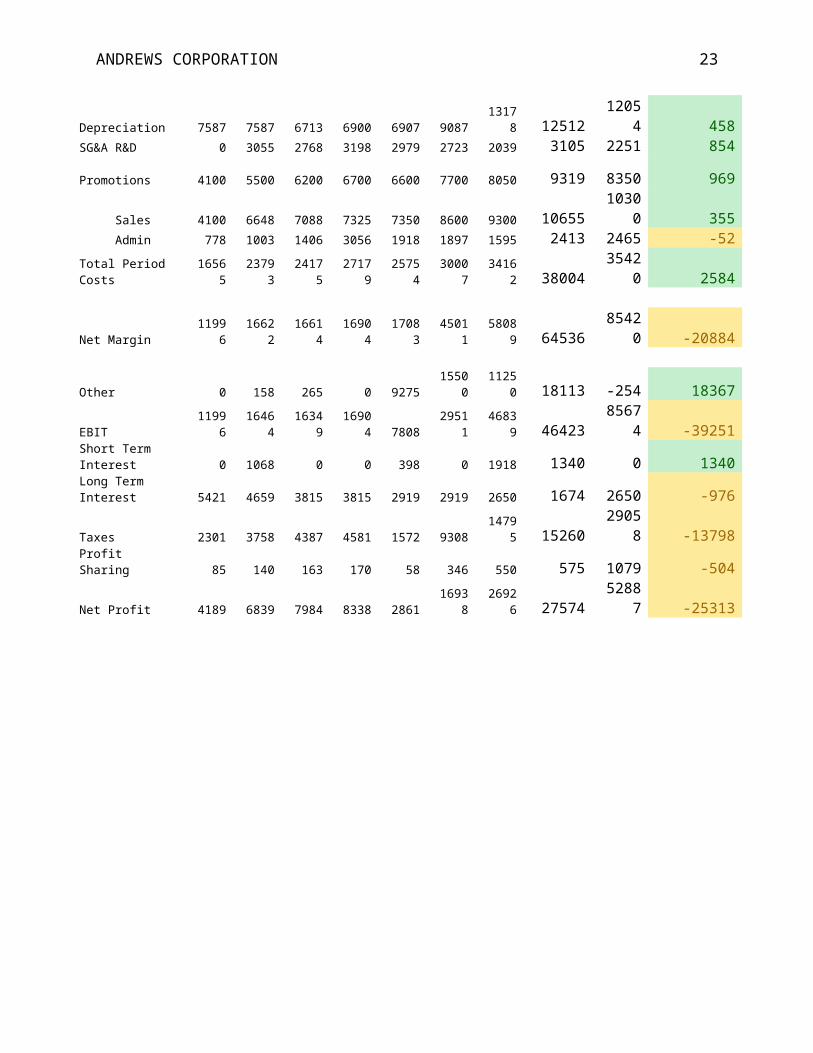
Projected Actual

Difference +/-

Income Statement 2014 2015 2016 2017 2018 2019 2020 2021 2021

Sales10107

311935

412771

416227

716183

221166

824168

7 27911327074

1 8372Variable Costs:

Direct Labor 28932 32726 38429 56089 57442 59698 59143 75004 50449 24555Direct Material 42546 45406 48385 62039 60745 76654 89349 100810 98799 2011Inventory Carry 1034 807 111 66 808 298 944 759 653 106Total Variable 72512 78939 86925 11819 11899 13665 14943 176573 14990 26672


4 5 0 6 1

Contribution Margin 28561 40415 40789 44083 42837 75018 92251 102540

120840 -18300

Period Costs:

Depreciation 7587 7587 6713 6900 6907 9087 13178 12512 12054 458SG&A R&D 0 3055 2768 3198 2979 2723 2039 3105 2251 854 Promotions 4100 5500 6200 6700 6600 7700 8050 9319 8350 969 Sales 4100 6648 7088 7325 7350 8600 9300 10655 10300 355 Admin 778 1003 1406 3056 1918 1897 1595 2413 2465 -52Total Period Costs 16565 23793 24175 27179 25754 30007 34162 38004 35420 2584

Net Margin 11996 16622 16614 16904 17083 45011 58089 64536 85420 -20884

Other 0 158 265 0 9275 15500 11250 18113 -254 18367EBIT 11996 16464 16349 16904 7808 29511 46839 46423 85674 -39251Short Term Interest 0 1068 0 0 398 0 1918 1340 0 1340Long Term Interest 5421 4659 3815 3815 2919 2919 2650 1674 2650 -976Taxes 2301 3758 4387 4581 1572 9308 14795 15260 29058 -13798Profit Sharing 85 140 163 170 58 346 550 575 1079 -504Net Profit 4189 6839 7984 8338 2861 16938 26926 27574 52887 -25313


Projected Actual

Difference +/-

Balance Sheet 2014 2015 2016 2017 2018 2019 2020 2021 2021Assets:

Cash 3434 20876 42055 38039 35988 32883 23758 37491 68154 -30663Accounts Receivable 8307 9810 10497 13338 13301 17397 19865 22943 22253 690Inventory 8617 6726 925 551 6736 2485 7864 6377 5444 933

Total Current Assets 20358 37412 53477 51928 56025 52765 51487 66811 95851 -29040

Plant & Equipment11380

011380

010070

011950

010360

013630

019767

2 19024218080

4 9438

Acc. Depreciation-

37933-

45520-

46994-

53893-

43787-

52873-

66052 -85293-

71948 -13345

Total Fixed Assets 75867 68280 53706 65607 59813 8342713162

0 10494910885

6 -3907

Total Assets 9622510569

210718

311753

511583

813619

218310

7 17176020470

7 -32947

Liabilities & O. Equity:

Accounts Payable 6583 4178 4439 6452 6817 7238 8431 9005 8045 960Current Debt 0 11359 0 0 4526 0 20850 0 0 0Long Term Debt 41700 34774 28020 28020 20850 20850 25000 25000 25000 0

Total Liabilities 48283 50311 32459 34472 32193 28088 54281 34005 33045 960

Common Stock 18360 18960 30319 30320 30319 40319 40319 40319 40319 0

Retained Earnings 29582 36421 44405 52743 53326 67785 88507 9743613134

3 -33907

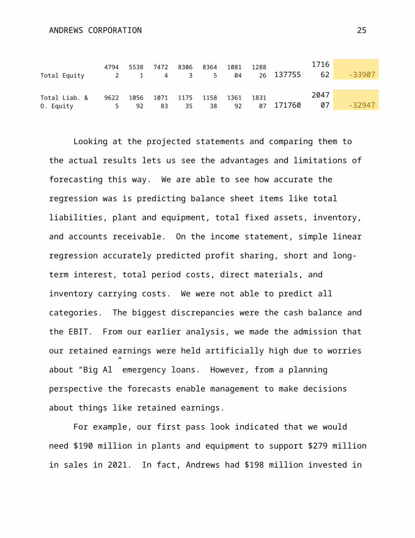
Total Equity 47942 55381 74724 83063 8364510810

412882

6 13775517166

2 -33907

Total Liab. & O. Equity 96225

105692

107183

117535

115838

136192

183107 171760

204707 -32947


Looking at the projected statements and comparing them to the actual results lets us see

the advantages and limitations of forecasting this way. We are able to see how accurate the

regression was is predicting balance sheet items like total liabilities, plant and equipment, total

fixed assets, inventory, and accounts receivable. On the income statement, simple linear

regression accurately predicted profit sharing, short and long-term interest, total period costs,

direct materials, and inventory carrying costs. We were not able to predict all categories. The

biggest discrepancies were the cash balance and the EBIT. From our earlier analysis, we made

the admission that our retained earnings were held artificially high due to worries about “Big Al”

emergency loans. However, from a planning perspective the forecasts enable management to

make decisions about things like retained earnings.

For example, our first pass look indicated that we would need $190 million in plants and

equipment to support $279 million in sales in 2021. In fact, Andrews had $198 million invested

in plants and equipment in 2020. Since no new investment in P & E is needed, Andrews might

look at ways of addressing the excessive amount it has in retained earnings. Investors expect a

company to retain earnings: retained earnings are often the fuel used to support growth, improve

efficiency, etc. However, if a company is not growing and is keeping significant amount of

earnings then they are going to demand a bigger dividend because the money they are allowing

the company to keep is not being used to make them more money (Leona). At this point in the

simulation, Andrews is growing and paying a dividend with a 2.5% yield. Since there are

thousands of types of sensors, Andrews might look to expand into a new type of sensor product

line or buy another firm in a new market segment.

Suppose though that Andrews had inside information in 2020, that two of its main

competitors would be exiting their shared market segment leaving Andrews with only three


competitors. Andrews CEO wants to capture 50% of the new opportunity. In 2020, the two

companies combined sales were $252,105 million. Andrews CEO targets $126,000 million in

new sales in addition to the $279,113 million already forecast for a grand total of $405,166

million dollars. The first thing he wants to know is how much capacity (Plants & Equipment) it

will take to support the new sales goal. In addition, the CEO wants a forecasted income

statement and balance sheet. The CFO agrees to have the figure together by the end of the day

and the statements by the end of the week. The CFO then goes to lunch and then plays golf since

he already has the necessary regression equations on file. For example, the regression equation

for Plants and Equipment: y = .5389x+39828. The CFO uses the calculator on his iPhone to see

that Andrews needs P & E assets of $258,172 million. In 2020, Andrews had P & E assets

totaling $197,672. Andrews would need to invest another $60,500 million to have the Plants and

Equipment necessary to support the new sales target. Andrews was projecting only $37,500

million in cash for 2021 leaving a shortfall of at least $23,000 million. The CFO reports all of

this to the CEO. (OK, I am not going to prepare another balance sheet and income statement for

you. You get the idea. I will put all the regression equations in the index.) Andrews’s CEO

now knows that to pursue the new market opportunity he needs to secure additional funds to

address the projected deficit in P & E of $23,000 million. The various historical regression

equations are then used by the CFO to complete the income statement and balance sheet.

ANDREWS CORPORATION

References

Brigham. (2017). Financial Management: Theory and Practice (14th ed.). Mason, Ohio: South-

Western.

Leona, Maluniu. (n.d.). How to Calculate Retained Earnings. Retrieved May 25, 2014, from

wikiHow Web site: http://www.wikihow.com/Calculate-Retained-Earnings

23

ANDREWS CORPORATION

Appendix A

Additional Information

Here are the simple linear equations used to calculate the projected balance sheet and

income statements. For simplicity I treated all costs as variable, which is an accepted though

more conservative technique. When the left and right side of the balance sheet did not balance I

made small adjustments, not statistically significant, in order to balance them. I did simple linear

regression for taxes, which would also not be done. I have also included a percent of sales EFN

worksheet.

Regression Equations

Balance Sheet Items:

.079x+15441 .0822x-.3451 .0035x+5401 .5389x+39828 -.234x-19981Cash Account Rec Inventory P/E Depreciation

.0228x+2641.7 .0787x-7401.5 -.1104x+46219 .1613x+3904.5 .3864x-8880.2Accounts P. Current Debt Long Term Debt Common Stock Retained Earnings

Income Statement Items:.2325x+10110

.3388x+6246.3

.0004x+647.82

.0358x+2519.4

.006x+1430.3

.0246x+2452.4

.0292x+2504.5

Direct laborDirect Material

inventory carry DPRE SG RD Promo sales

.0063x+654.72.1091x-12338.1 .0072x-670.08 -.0175x+6558.19 .0799x-7040.83 .003x-262.11

admin other short int long int TX PS

24


External Funds Needed Work Sheet

S0 = Current Sales,

S1 = Forecasted Sales = S0(1 + g),

g = the forecasted growth rate is Sales,

A*0 = Assets (at time 0) which vary directly with Sales,

L*0 = Liabilities (at time 0) which vary directly with Sales,

PM = Profit Margin = (Net Income)/(Sales), and

b = Retention Ratio = (Addition to Retained Earnings)/(Net Income).

Sales Forecast (S1): S0 g S1

241687 0.155 405166

PM NI Sales PM149435 241687 0.6183

b ARE NI88507 149435 0.592278

A0 51487

S0 241687 0.213032

S1 405166

S0 241687 163479 34826.21

A0 - Depreciation A0 Depreciation

A0 25000 13000 12000

L0 7000

S0 241687 0.028963

S1 405166

S0 241687 163479 4734.855


PM 0.075

S1 405166b 0.592277579 17997.81

EFN: 24093.55

The EFN equation shows a positive number of $24,094 million in external financing

needed to support the projected level of sales. Once again, this is a first pass look. There are

many other factors to be considered.

ANDREWS CORPORATION

Author Note

I got the idea to calculate the financial ratios manually after discovering that I was unsure

as to what drove each ratio. It is one thing to look the statistic for the current ratio and a whole

other thing to know that the current ratio is found by dividing current assets by current liabilities.

Moreover, a high current ratio indicates that a firm’s current assets are growing faster than its

liabilities. Conversely, a firm that is having financial difficulty will start to pay its bills more

slowly and its liabilities will grow lowering the ratio. Understanding the ratios and what drives

the ratios them allowed Team Andrews to make decisions we otherwise would not have made.

For example, Andrews P/E ratio was 14.89 in 2017, meaning that investors were willing to pay

$14.89 for every dollar of earnings. Investors were willing to pay industry $22.15 for every

dollar of earnings to industry. Why were investors willing to pay more to industry than to

Andrews? The answer is that P/E ratios are higher for firms with strong growth prospects and

lower for riskier firms. In fact, 2018 proved to be one of Andrews’s leanest years; we recorded

our smallest profit of the simulation. The situation was that our contribution margin was

shrinking after four rounds of price cuts, we were constrained by capacity, and we had not

automated. Therefore, we sold our traditional product and used the proceeds to launch a new

high-end product. We also, sold some of our excess capacity in our smaller product lines and

bumped up automation a bit. We would not have made these decisions had we not learned what

drove the P/E ratio.

All mistakes in this document are the author's alone.

27

Documents

Liquidity Ratiostalentbucket.weebly.com/.../andrews_corporation.docx · Web viewThis would require increasing capacity, spending money on marketing, etc. (all of which would lower