Embed Size (px)
Citation preview

Liquidity, Interest Rates and House Prices in the Euro area: A DSGE
Analysis
Margarita Rubio∗
University of Nottingham
José A. Carrasco-Gallego†
University of Portsmouth
October 2015
Abstract
In this paper, we propose a two-country monetary union DSGE model with housing, in order to
study how different shocks contributed to the increase in housing prices and credit in the EMU prior
to the crisis. One of the countries is calibrated to represent the core group in the Euro area while
the other one corresponds to the periphery. First, we explore how a liquidity shock (or a decrease in
the interest rate) affects house prices and the real economy through the asset price and the collateral
channel. Then, we analyze how a house price shock in the periphery and a technology shock in the
core countries are transmitted to the both economies. We find that a combination of an increase
in liquidity in the Euro area coming from the common monetary policy, together with asymmetric
house price and technology shocks, can explain the increase in house prices in the Euro area and the
stronger credit growth in the peripheral economies in the pre-crisis period.
Keywords: Liquidity, interest rates, monetary policy, house prices, collateral effects, asymmetric
shocks, asset prices.
JEL Classification: E32, E44, E58
∗University of Nottingham, Sir Clive Granger Building, University Park, Nottingham, NG7 2RD, UK. E-mail: [email protected].†Portsmouth Business School, 0.21 Burnaby Terrace, Burnaby Rd., Portsmouth PO1 3DE, UK. E-mail. jose.carrasco-
1

"[...] developments in the monetary aggregates and credit play an important role in the development
of asset price boom episodes. Although the issue of empirical causality between asset prices on the one
hand and money and credit developments on the other is a complicated one, the potential role of credit
and money in driving asset prices is straightforward.". Speech by Jean-Claude Trichet, President of the
ECB. 8 June 2005, Singapore.
1 Introduction
The launch of the European Economic and Monetary Union (EMU) in 1999 built up large imbalances in
housing markets between European countries. In particular, we can distinguish two groups of countries:
the peripheral countries (Greece, Ireland, Italy, Portugal, and Spain, known as GIIPS) and the rest.1
One of these imbalances was set in the real sector when residential property prices of new and existing
houses and flats increased 80% in the periphery from 1999 to 2007, while in the core the increase was
less than 20%. Moreover, real gross fixed capital formation in dwellings doubled in the periphery and
stated the same in the core between both years. Additionally, mortgage loans grew moderately in the
core but they boomed in the periphery (Brzoza-Brzezina, Kolasa and Makarski, 2014).
Several scholars have pointed the possibility that the main drivers of the asymmetric evolution of
the housing prices between the two areas could be of different nature. The first driver may remain
in the financial sector: a fall in interest rates following their euro area accession and the easy access
to cross-border borrowing after the launch EMU (see for instance ECB, 2003; Honohan and Leddin
2006; Blanchard, 2007; or Andrés et al., 2013). Secondly, it could be possible that a house price bubble
was developed in the periphery. Finally, a third possibility might be in the real economy: shocks to
productivity with asymmetric distribution between core and periphery (Andrés et al., 2013).
With respect to the first driver, it is important to note that in the Euro area, monetary policy is
common for all the countries and it is conducted by the European Central Bank (ECB). The ECB
implemented, since the introduction of the Euro till 2006, an expansionary monetary policy which
increased liquidity in the Euro area (See Figure A1 in the Appendix). This fact was reflected in decreasing
the interest rate to unprecedented lows. The fall was even more dramatic if the pre-EMU interest rates
are taken into account.2 Furthermore, due to the significant differences between the core and periphery
1See Quint and Rabanal (2014) for more details on this division.2For instance, the average Spanish government interest rate (interest payments/sovereign debt stock) fell from around
9% in the late 1990s to below 4% by 2010.
2

economies, the common monetary policy could have an asymmetric impact. The domestic demand
growth was extremely strong at the periphery but very weak at the core. Therefore, monetary policy
was too loose for the periphery and too tight for the rest. The increase in liquidity, the reduction of the
interest rate, and its asymmetric impact caused different effects on the housing prices and credit in the
core and the periphery through the transmission channels of monetary policy.
Secondly, many of the peripheral countries experimented strong increases in housing demand, not
determined by economic fundamentals, which can be interpreted as housing bubbles or asymmetric house
price shocks.
The third driver, an asymmetric productivity shock, could also affect differently the house prices of
the core and the periphery. The productivity in the core evolved better than in the periphery.3 Even
though the peripheral productivity was not improving as much as in the core, those countries benefitted
from the lower common interest rates stemming from low inflation in the more productive region. This
created a demand shock that affected credit and house prices in the periphery.
In order to explore the three previous drivers, we develop a model with two countries inside a
monetary union. We identify these countries as core and periphery, respectively. In each country,
there are two sectors, construction and consumption, and two infinite-horizon households, savers and
borrowers. The model constitutes a two-country version of the seminal paper of Iacoviello (2005), that
introduces a financial accelerator that works through the housing sector. This is done in the spirit of
Iacoviello and Smets (2006) and Aspachs and Rabanal (2010). However, it introduces cross-country
housing-market heterogeneity as in Rubio (2014). The model is then adapted to represent the core
and the periphery in the Euro area, as in Brzoza-Brzezina et al (2014) and Quint and Rabanal (2014),
who, differently to us, use their framework to study how to implement macroprudential policies in these
two regions. In our paper, we use this model to analyze the influence of interest rate falls (increase in
liquidity), and productivity shocks, on the asymmetric evolution of housing prices in the core and the
periphery. Additionally, we study the impact of a shock in house prices that some scholars, such as in’t
Veld et al. (2012), have pointed as source of changes in fundamentals.
Results from our simulations show that the increase in liquidity can explain higher house prices,
through an asset price channel. Furthermore, collateral effects coming from higher house prices, con-
tributed to the credit boom in the Euro area, being the effects more remarkable in the periphery, given
that these countries were more leveraged. We also consider a house price shock in the periphery, to
3See Figure A2 in the Appendix.
3

account for a housing bubble in this area. We see that a stronger housing demand preference in these
economies increases credit by a large amount, through the collateral constraint of borrowers. Finally, we
observe that higher productivity in the core makes the common interest rate decrease and this causes a
demand shock in the periphery, making credit and house prices increase through the credit channel.
Summarizing, our analysis shows that the combination of an increase in liquidity in the Euro area
coming from the common monetary policy, together with asymmetric house price and technology shocks,
contributed to the increase in house prices in the Euro area and the stronger credit growth in the
peripheral economies in the pre-crisis period.
The paper is organized as follows. Section 1.2 presents some discussion on the related literature and
the contribution of the paper. Section 2 sets up the model. Section 3 simulates the model. Section 4
concludes.
1.1 Related Literature and Contribution
There are a number of empirical studies that study the interrelations between monetary policy, liquidity
and other shocks with house prices and credit. For instance, Taltavull and White (2012, 2015) use a
VECM to examine the influence of several economic variables, including liquidity on house prices for
the UK and Spain. Crowe et al. (2011) study the relationship between monetary policy conditions and
house price changes based on a panel vector autoregression. Adrian and Shin (2009) and De Nicolo et al.
(2010) analyze to which extent monetary policy affects the leverage in the financial sector. Our paper
provides a theoretical counterpart to this studies to disentangle the mechanisms behind those results
through a DSGE model.
On the other hand, there is also plenty of evidence that housing and credit markets did not be-
have in the same way across European countries. Guerrieri and Esposito (2012) provide evidence of
these imbalances. They notice that the demand boom in the peripheral countries, led to losses of com-
petitiveness and asset price inflation, notably in the housing market. Hansen (2010) and Marin (2010)
suggest that Germany and the core countries reduced their labour costs, following the launch of the Euro
and increased their productivity. Furthermore, as Stockhammer (2011) shows the core economies were
export-led while the peripheral were credit-led. In the periphery, credit-financed consumption growth
and residential investment became the key source of demand growth and run substantial current account
deficits. Besides, the core did not experience an equally strong rise in household debt and consumption
and increasingly relied on exports as the main growth engine. Also, as pointed out by Quint and Rabanal
4

(2014), the leverage in the housing sector was much higher in the periphery than in the core countries.
The increase in household debt in percentage of GDP from 2000 to 2008 was more than 32% in Spain,
61% in Ireland, 21% in Portugal and 18% in Italy; while in core countries was much lower, in Austria
was 7% and in Germany 11%.4
Our paper also sheds some light, from a theoretical perspective, on the effects of these imbalances.
We calibrate the model to be representative of the core and the peripheral group and characterize
asymmetric house price shocks (in the periphery) and asymmetric productivity shocks (in the core),
to account for this evidence and find the mechanisms that explain them. We approximate the more
leveraged countries by a higher LTV, which makes the collateral constraint more important and the
financial accelerator effects stronger. In this way, the model is able to capture this difference between
the two areas. Furthermore, since it is a two country model within a monetary union, the analysis is
also able to illustrate the asymmetric technology and house price shocks between these two regions and
the common monetary policy. Therefore, the structure of the model is suitable to answer the research
question that we propose.
We introduce several channels in the setting through which shocks are transmitted. Throughout the
paper, we consider liquidity shocks and changes in the interest rate as equivalent. As Woodford (2003)
and Michis (2014) show, interest rates are influenced mainly by the money supply (i.e., the liquidity
effect). Then, a change in the interest rate or in the liquidity can affect real estate prices via different
channels. The first channel is the credit channel (Mishkin, 2007). Lower interest rates make it cheaper
to obtain a mortgage and thus, there is an increase in the housing demand and an increase in the
housing prices. This channel is present in our model through borrower’s debt repayments. The second
channel is the so-called asset inflation channel (Belke et al, 2008). In this case, lower interest rates imply
higher asset prices, including housing prices. In our model, housing prices move inversely with interest
rates. Another channel that we explore here is the impact of house prices in the economy. Our model
captures the positive wealth effect in case that the real estate price increases, since borrowers use houses
as collateral to obtain loans. A higher price will let them increase their purchases, including houses.
Therefore, we have here a financial accelerator effect (See Aoki et al, 2004 or Iacoviello, 2005).
Therefore, in our paper, we analyze the influence of interest rate falls (increase in liquidity), and
productivity shocks, on the asymmetric evolution of housing prices in the core and the periphery. Ad-
ditionally, we also study the impact of a shock in house prices.
4See Stockhammer (2011)
5

2 Model Setup
We consider an infinite-horizon, two-country, two-sector economy inside a monetary union. The home
country (Core) is denoted by COR and the rest of the union (the periphery) by PER. Households
consume, work, and demand real estate. Each country produces one differentiated intermediate good,
but households consume goods from both countries. For simplicity, housing is a non-traded good. We
assume that labor is immobile across the countries. Firms follow a standard Calvo problem. In this
economy, both final and intermediate goods are produced. Prices are sticky in the intermediate-goods
sector. There is a construction sector that produces houses. We introduce transaction-facilitating money
by the device of including real balances as an argument of each household’s utility function. Monetary
policy is conducted by a single central bank that responds to a weighted average of inflation in both
countries. We allow for housing-market heterogeneity across the countries.
2.1 The Consumer’s Problem
There are two types of consumers in each country: borrowers and savers. Borrowers are constrained
individuals who need to collateralize their debt repayment, that is, interest payments in the next period
cannot exceed a proportion of the expected future value of the current house stock. As in Iacoviello
(2005), I assume that constrained consumers are more impatient than unconstrained ones.5
2.1.1 Unconstrained Consumers (Savers)
Unconstrained consumers in COR maximize as follows:
max E0
∞∑t=0
βt(
lnCt + j lnHt + χ lnmt −(Lut )η
η
), (1)
Here, E0 is the expectation operator, β ∈ (0, 1) is the discount factor, and Ct, Ht, mt, and Lt are
consumption at t, the stock of housing, real money balances and hours worked, respectively.6 j represents
the weight of housing in the utility function. 1/ (η − 1) is the aggregate labor-supply elasticity.
Consumption is a bundle of domestically and foreign-produced goods, defined as: Ct = (CCORt)n (CPERt)
1−n ,
where n is the size of COR. Unconstrained consumers provide labor to both the consumption and con-
struction sector, so that Lt =[(Lct)
1−ν + (Lht)1−ν] 11−ν
.
5This assumption ensures that the borrowing constraint is binding in the steady state and that the economy is endoge-nously split into borrowers and savers.
6 It is assumed that housing services are proportional to the housing stock.
6

The budget constraint for COR is as follows:
PCORtCCORt + PPERtCPERt +QCORt (Ht −Ht−1) +RCORt−1Bt−1 +Rt−1Dt−1 +ψ
2D2t +Mt−1 ≤
WctLct +WhtLht +Bt +Dt +Mt−1 + PCORtFt + PCORtTt, (2)
where PCORt and PPERt are the prices of the goods produced in Countries COR and PER, respectively,
QCORt is the housing price in COR, and Wct and Wht are the consumption and housing sector wages for
unconstrained consumers. Bt represents domestic bonds denominated in the common currency. RCORt is
the nominal interest rate in COR. Positive bond holdings signify borrowing, and negative signify savings.
However, as we will see, unconstrained consumers will choose not to borrow at all: they are the savers
in this economy. Dt are foreign-bond holdings by savers in COR.7 Mt are nominal money balances. Rt
is the nominal rate of foreign bonds, which are denominated in euros. As is common in the literature,
to ensure stationarity of net foreign assets we introduced a small quadratic cost of deviating from zero
foreign borrowing, ψ2D2t .8 Savers obtain interest on their savings. Ft are lump-sum profits received from
the firms. Tt are lump-sum government transfers.
Dividing by PCORt, we can rewrite the budget constraint in terms of goods in COR:
CCORt +PPERtPCORt
CPERt + qCORt (Ht −Ht−1) +RCORt−1bt−1
πCORt+Rt−1dt−1PCORt
+ψ
2d2t +
mt−1πCORt
≤
wctLct + whtLht + bt + dt +mt + Ft + Tt, (3)
where πCORt denotes inflation for the goods produced in COR, defined as PCORt/PCORt−1. qCORt is
defined as QCORt/PCORt.
Maximizing (1) subject to (3) , we obtain the first-order conditions for the unconstrained group:
CCORtCPERt
=nPPERt
(1− n)PCORt(4)
1
CCORt= βEt
(RCORt
πCORt+1CCORt+1
), (5)
7Savers have access to international financial markets.8See Iacoviello and Smets (2006) for a similar specification of the budget constraint.
7

1− ψdtCCORt
= βEt
(Rt
πCORt+1CCORt+1
), (6)
n
CCORt= βEt
(n
πCORt+1CCORt+1
)+
χ
mt, (7)
wct = (Lt)η−1 (Lct)
−ν[(Lct)
1−ν + (Lht)1−ν] ν1−ν CCORt
n, (8)
wht = (Lt)η−1 (Lht)
−ν[(Lct)
1−ν + (Lht)1−ν] ν1−ν CCORt
n, (9)
j
Ht=
n
CCORtqCORt − βEt
n
CCORt+1qCORt+1. (10)
Equation (4) equates the marginal rate of substitution between goods to the relative price, and it reflects
the fact that countries are trading. Equation (5) is the Euler equation for consumption, which states that
consumers would like to smooth consumption over time. That is, at the margin, consumers should be
indifferent between consuming one extra unit of consumption today or saving it to the future. Equation
(6) is the first-order condition for net foreign assets, and its intuition is equivalent to the previous Euler
equation. Equation (7) represents money demand, that is an Euler equation for money.9 Equations (8)
and (9) are the labor-supply conditions for both sectors. These equations are standard. Equation (10)
is the Euler equation for housing and states that, at the margin, the benefits from consuming housing
today have to be equal to the costs. That is, if consumers consume one unit of housing today, they enjoy
the utility it derives and they can sell it in the future. However, they incur in a cost today in terms of
consumption.
Combining (5) and (6) we obtain a non-arbitrage condition between home and foreign bonds:10
RCORt =Rt
(1− ψdt). (11)
9The Euler condition for money is a typical expression for the price of an asset. If consumers give up consumption todayand decide to hold money forever from then on, they will enjoy the stream of utility services which will be eroded from therise in prices.10The log-linearized version of this equation could be interpreted as the uncovered interest-rate parity.
8
Since all consumption goods are traded and there are no barriers to trade, we assume in this paper
that the law of one price holds:
PCORt = P ∗CORt, (12)
where variables with a star denote foreign variables.
2.1.2 Constrained Consumers (Borrowers)
Constrained consumers are more impatient than unconstrained ones, that is β̃ < β. Constrained con-
sumers face a collateral constraint: the expected debt repayment in the next period cannot exceed a
proportion of the expectation of tomorrow’s value of today’s stock of housing:
EtRCORtπCORt+1
b′t ≤ kCOREtqCORt+1H
′t , (13)
where equation (13) represents the collateral constraint for the borrower. kCOR can be interpreted
as the loan-to-value ratio in COR.
Borrowers maximize their lifetime utility function:
max E0
∞∑t=0
β̃t
lnC′t + j lnH
′t + χ lnm′t −
(L′t
)ηη
, (14)
where C′t =
(C′CORt
)n (C′PERt
)1−n, L′t =
[(L′ct
)1−ν+(L′ht
)1−ν] 11−ν
, subject to the budget constraint
(in terms of the consumption good in COR):
C ′CORt +PPERtPCORt
C′PERt + qCORt
(H′t −H
′t−1
)+RCORt−1b
′t−1
πCORt+m′′t−1
πCORt≤ w′ctL
′ct +w
′htL
′t + b
′t +m
′t, (15)
and subject to the collateral constraint (13).
The first-order conditions for these consumers are as follows:
C′CORt
C′PERt
=nPPERt
(1− n)PCORt(16)
9
n
C′CORt
= β̃Et
(nRCORt
πCORt+1C′CORt+1
)+ λtRCORt, (17)
n
C′CORt
= β̃Et
(n
πCORt+1C′CORt+1
)+
χ
m′t, (18)
w′ct =
(L′t
)η−1 (L′ct
)−ν [(L′ct
)1−ν+(L′ht
)1−ν] ν1−ν C
′CORt
n, (19)
w′ht =
(L′t
)η−1 (L′ht
)−ν [(L′ct
)1−ν+(L′ht
)1−ν] ν1−ν C
′CORt
n, (20)
j
H′t
=n
C′CORt
qCORt − β̃Etn
C′CORt+1
qCORt+1 − λtkCOREtqtCOR+1πCORt+1. (21)
These first-order conditions can be interpreted in a similar way to the ones of the savers. However,
they differ from those of unconstrained individuals in some aspects. In the case of constrained consumers,
the Lagrange multiplier on the borrowing constraint (λt) appears in equations (17) and (21) to reflect
the fact that housing has an extra collateral effect on these consumers. As in Iacoviello (2005), the
borrowing constraint is always binding, so that constrained individuals borrow the maximum amount
they are allowed, and their saving is zero.11
The problem for consumers is analogous in PER.
2.2 Firms
2.2.1 Final-Consumption Goods Producers
In COR, there is a continuum of final-goods producers that aggregate intermediate goods according to
the production function:
Y kCORt =
[∫ 1
0Y kCORt (z)
ε−1ε dz
] εε−1
, (22)
11From the Euler equations for consumption of the unconstrained consumers, we know that RCOR = 1/β , where variableswithout a time subscript denote steady-state variables. If we combine this result with the Euler equation for consumption
for the constrained individual, we have λ = n(β − β̃
)/C
′COR > 0. Given that β > β̃, the borrowing constraint holds with
equality in steady state. Since the model is log-linearized around the steady state and low uncertainty is assumed, thisresult can be generalized to off-steady-state dynamics.
10

where ε > 1 is the elasticity of substitution among intermediate goods.
The total demand of intermediate-good z is given by YCORt (z) =(PCOR(z)PCORt
)−εYCORt, and the price
index is PCORt =[∫ 10 PCORt (z)1−ε dz
] 1ε−1
.
2.2.2 Intermediate-Goods and House Producers
The intermediate-goods consumption market is monopolistically competitive. Following Iacoviello (2005),
intermediate goods are produced according to the following production function:
YCORt (z) = ξt (Lct (z))γ(L′ct (z)
)(1−γ), (23)
where ξt represents technology. We assume that log ξt = ρξ log ξt−1 + uξt, where ρξ is the autoregressive
coeffi cient and uξt is a normally distributed shock to technology. γ ∈ [0, 1] measures the relative size of
each group in terms of labor.
Symmetry across firms allows avoiding index z and re-writing equation (23) as:
YCORt = ξt (Lct)γ(L′ct
)(1−γ), (24)
The production function for housing investment is as follows:
ICORt = ξt (Lht)γ(L′ht
)(1−γ), (25)
Producers maximize profits:
maxLct,Lht,L
′ct,L
′ht
YCORtXt
+ qCORtICORt − wctLct − whtLht − w′ctL
′ct − w
′htL
′t. (26)
The first-order conditions for labor demand are the following:
wct =1
XtγYCORtLct
, (27)
w′ct =
1
Xt(1− γ)
YCORt
L′ct
, (28)
wht = γqCORtICORt
Lht, (29)
11

w′ht = (1− γ)
qCORtICORt
L′ht
, (30)
where Xt is the markup, or the inverse of marginal cost.
The price-setting problem for the intermediate-goods producers is a standard Calvo-Yun case. An
intermediate-goods producer sells goods at price PCORt (z) , and 1− θ is the probability of being able to
change the sale price in every period. The optimal reset price POPTCORt (z) solves the following:
∞∑k=0
(θβ)k Et
{Λt,k
[POPTCORt (z)
PCORt+k− ε/ (ε− 1)
Xt+k
]Y OPTCORt+k (z)
}= 0. (31)
The aggregate price level is given as follows:
PCORt =[θP 1−εCORt−1 + (1− θ)
(POPTCORt
)1−ε]1/(1−ε). (32)
Using (31) and (32) and log-linearizing, we can obtain the standard forward-looking Phillips curve.12
The firm problem is similar in PER.
2.3 Aggregate Variables and Market Clearing
Economy-wide aggregates in Country COR are Ct ≡ Ct + C′t, Lt ≡ Lt + L
′t. Domestic housing market
clearing requires ICORt ≡ (Ht −Ht−1) +(H′t −H
′t−1
).
The market clearing condition for the final good in Country COR is nYCORt = nCCORt+(1− n)C∗CORt+
nψ2 d2t . Domestic financial markets clear: bt = b
′t. The world bond market clearing condition is
ndt + (1− n) PPERtPCORtd∗t = 0, where dt denotes the foreign bonds in real terms. The net foreign asset
position follows dt = Rt−1(1−ψdt)πCORtdt−1 + YCORt − CCORt − PPERt
PCORtCPERt. Everything is similar in PER.
2.4 Monetary Policy
In order to close the model, we need to specify a way to introduce monetary policy. The central bank
uses the money supply as an instrument to affect the economy, so that injecting or draining liquidity into
the system is transmitted through credit and housing markets until it affects real variables. However, if
we combine the saver’s Euler equation for consumption (equation 5) with their money demand (equation
7), we observe the following:
12This Phillips curve is consistent with other two-country models with financial accelerator. See for instance Gilchrist etal (2002) or Iacoviello and Smets (2006).
12

mt =χCCORt
n
(RCORt
RCORt − 1
)That is, for given values of consumption and prices and taking into account equation (11), there is a
one-to-one mapping between the money supply and the interest rate set by the central bank. Therefore,
monetary policy can be represented by an interest rate rule. In this way, a decrease in the target interest
rate is equivalent to an increase in liquidity and vice versa. With this approach, although there would
be a transaction-oriented demand for real money balances implied by the optimization problem of the
agents, when policy is based on an interest rate policy rule, the money demand function would serve
only to indicate the quantity of money needed to support the interest rate rule. Thus, throughout the
paper we will assume that interest rate shocks are analogous to liquidity shocks.13
2.4.1 Interest Rate Rule
We consider a Taylor rule with interest-rate smoothing for interest-rate setting by a single central bank,14
Rt = (Rt−1)ρR
([(πCORt)
n (πPERt)(1−n)
](1+φπ)R
)1−ρRεR,t, (33)
0 ≤ ρR ≤ 1 is the parameter associated with interest-rate inertia. (1 + φπ) measures the sensitivity of
interest rates to current inflation. εR,t is a white noise shock process with zero mean and variance σ2εR.
This rule is consistent with the primary objective of the ECB being price stability.
3 Dynamics
In this section, we simulate the model to illustrate how monetary policy affects housing prices and the
rest of economic variables in the core and the periphery. In particular, we want to explore how an increase
in liquidity has affected housing markets and the real economy in both economies. We also illustrate the
effects of house price shocks and technology shocks in the periphery and the core economies, respectively.
13Since Woodford (2003), the standard practice is to consider a cash-less economy, expressing policy behavior in termsof interest rate rules.14This type of rule is also used in other monetary-union models. See Iacoviello and Smets (2006) or Aspachs and Rabanal
(2008). Furthermore, as shown in Iacoviello (2005) and Rubio and Carrasco-Gallego (2013), a rule that only responds toinflation enhances the financial accelerator.
13

3.1 Parameter Values
Parameters are calibrated to reflect the core economy and the periphery. Some of the parameters are
standard and are common for both economies and some others will be specifically calibrated for each
area.15
Discount factors are set to be common in both economies, following the standard values in the
literature. The discount factor for savers, β, is set to 0.99 so that the annual interest rate is 4% in steady
state. The discount factor for borrowers, β̃, is set to 0.98.16 The steady-state weight of housing in the
utility function, j, is set to 0.12. This parameter pins down the ratio of housing wealth to GDP.17 We set
η = 2, implying a value of the labor supply elasticity of 1.18 Following Horvath (2000) and Iacoviello and
Neri (2010), we set the inverse elasticity of substitution across hours in the two sectors to one. For the
loan-to-value ratio we consider a steady-state value of 0.70 and 0.80, for COR and PER, respectively,
in order to reflect a low and a high leveraged country.19 The labor-income share of unconstrained
consumers, γ, is set to 0.7.20 We pick a value of 6 for ε, the elasticity of substitution among intermediate
goods. This value implies a steady-state markup of 1.2. The probability of not changing prices, θ, is set
to 0.75, implying that prices change every four quarters on average. For the Taylor Rule parameters,
we use ρ = 0.8, φπ = 0.5. The first value reflects a realistic degree of interest-rate smoothing.21 φπ is
consistent with the original parameters proposed by Taylor in 1993. The size of the peripheral group is
considered to be 40%.22 A technology shock is a 1% positive technology with 0.9 persistence.23
14
2 4 6 8 100.5
0
0.5
1Consumption
%de
v. s
tead
y st
ate
2 4 6 8 101
2
3
4Mortgaged Houses
2 4 6 8 100.5
0
0.5
1House Prices
%de
v. s
tead
y st
ate
2 4 6 8 100
2
4
6Borrowing
2 4 6 8 100.2
0
0.2Interest Rate
quarters
%de
v. s
tead
y st
ate
2 4 6 8 100
0.2
0.4Inflation
quarters
CORPER
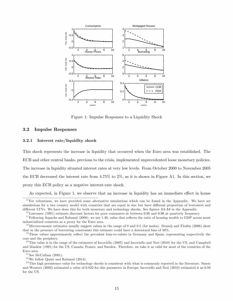
Figure 1: Impulse Responses to a Liquidity Shock
3.2 Impulse Responses
3.2.1 Interest rate/liquidity shock
This shock represents the increase in liquidity that occurred when the Euro area was established. The
ECB and other central banks, previous to the crisis, implemented unprecedented loose monetary policies.
The increase in liquidity situated interest rates at very low levels. From October 2000 to November 2005
the ECB decreased the interest rate from 4.75% to 2%, as it is shown in Figure A1. In this section, we
proxy this ECB policy as a negative interest-rate shock.
As expected, in Figure 1, we observe that an increase in liquidity has an immediate effect in house
15For robustness, we have provided some alternative simulations which can be found in the Appendix. We have setsimulations for a two country model with countries that are equal in size but have different proportion of borrowers anddifferent LTVs. We have done this for both monetary and technology shocks. See figures A3-A6 in the Appendix.16Lawrance (1991) estimate discount factors for poor consumers at between 0.95 and 0.98 at quarterly frequency.17Following Aspachs and Rabanal (2008), we use 1.40, value that reflects the ratio of housing wealth to GDP across most
industrialized countries as a proxy for the Euro area.18Microeconomic estimates usually suggest values in the range of 0 and 0.5 (for males). Domeij and Flodén (2006) show
that in the presence of borrowing constraints this estimate could have a downward bias of 50%.19These values approximately reflect the prevalent loan-to-values in Germany and Spain, representing respectively the
core and the periphery.20This value is in the range of the estimates of Iacoviello (2005) and Iacoviello and Neri (2010) for the US, and Campbell
and Mankiw (1991) for the US, Canada, France, and Sweden. Therefore, we take it as valid for most of the countries of theEuro area.21See McCallum (2001).22We follow Quint and Rabanal (2014).23This high persistence value for technology shocks is consistent with what is commonly reported in the literature. Smets
and Wouters (2002) estimated a value of 0.822 for this parameter in Europe; Iacoviello and Neri (2010) estimated it as 0.93for the US.
15

prices. As stated before, there are several channels that can potentially link liquidity with house prices.
Through the asset-price channel, since the increase in liquidity lowers the interest rate, asset prices
should increase due to a substitution effect from money to other assets. House prices are an asset price
and therefore they should move inversely with the interest rate. Figure 1 shows that this is precisely
what happens; following the decrease in the interest rate, house prices start to rise. We also see that
loose credit conditions in the Euro area lead to an increase in borrowing, especially in the periphery.
There are two reasons why this occurs. First, lower interest rates make it cheaper to obtain a mortgage
and thus, the common lower interest rates makes credit increase in both the core and the periphery.
A second reason which represents a strong mechanism in this model is wealth effects. Borrowers need
housing collateral in order to obtain loans. The value of this collateral is thus linked to house prices since
houses will be more or less valuable depending on house price movements. As we have seen, the increase
in liquidity makes house prices go up and therefore the value of the collateral to increase as well. This
produces a wealth effect because borrowers are wealthier now, since they can obtain more credit either
to purchase more houses or more consumption goods. This collateral channel is the so-called financial
accelerator effect since changes due to non-financial reasons, such as liquidity in this case, are amplified
through the financial market. We also see that the fact that the LTV is higher in the periphery makes
these households be more sensitive to changes in the interest rate, due to a stronger financial accelerator
effect. The increase in liquidity causes a common demand shock in both areas but it exacerbates the
credit boom in the periphery. Mortgaged houses, although they increase in both areas, increase by more
in the peripheral economies. This increase in housing demand should also have an effect on house prices.
However, as we see in the graph, house prices do not increase by more in the periphery than in the core
countries. Thus, given that the increase in house prices is very similar in the two economies, we can
conclude that the channel that is prevalent here is the asset price channel, which is common for both
the core and the periphery. In terms of consumption, demand increases in both groups of countries due
to lower interest rates and the collateral effects, but by more in the periphery.
3.2.2 House price shock in PER
In order to explain the higher house price growth in the peripheral economies, we assume that the
periphery suffered a housing demand shock that was translated to higher house prices. Brzoza-Brzezina
et al. (2014) present evidence that residential property prices of new and existing houses and flats in the
periphery raised to 80% between 1999 and 2007, while in the core the increase was less than 20%. They
16

2 4 6 8 100.02
0.01
0
0.01Consumption
%de
v. s
tead
y st
ate
2 4 6 8 102
0
2
4Mortgaged Houses
2 4 6 8 100
0.5
1
1.5House Prices
%de
v. s
tead
y st
ate
2 4 6 8 100
2
4
6Borrowing
2 4 6 8 102
1
0x 103 Interest Rate
quarters
%de
v. s
tead
y st
ate
2 4 6 8 105
0
5x 10³ Inflation
quarters
CORPER
Figure 2: Impulse Responses to a House Price Shock in the Periphery
also show that real gross fixed capital formation in dwellings multiplied by two in the periphery and
stated the same in the core in that period. Furthermore, they display that mortgage loans boomed in
the periphery while they grew moderately in the core. Besides, Mayer and Gareis (2013) find that in the
EMU from 1997 to 2008 housing preference and technology shocks were the main drivers of fluctuations
in house prices and residential investment. They show that the majority of the variation of housing
preference shocks can be explicated by demand factors. There is a general consensus about the fact that
some periphery countries suffered a bubble on house prices during the first years of the 21st century.24
Therefore, in order to explain the higher house price growth in the peripheral economies, we first analyze
the situation in which the periphery suffers a housing demand shock that is translated to higher house
prices. In the next section we will consider a technology shock.
Figure 2 illustrates an increase in the preference for houses in the periphery produces a raise in
housing prices in this area. Since the value of the collateral is higher in the peripheral economies but not
in the core countries, borrowing increases only in the periphery, creating a credit boom in this region.
Houses, in the periphery, since they serve as a collateral, have an intrinsic value that consumption goods
do not have. Therefore, in the periphery, households substitute away consumption goods by mortgaged
houses. This is why we observe a strong increase in mortgaged houses, financed by the increase in
credit and a slight decrease in consumption. The common interest rate slightly falls in the monetary
24See for instance McQuinn and O’Reilly (2006), Malzubris (2008) or Conefrey and Gerald (2010).
17

2 4 6 8 100
0.2
0.4Consumption
%de
v. s
tead
y st
ate
2 4 6 8 100.5
0
0.5
1Mortgaged Houses
2 4 6 8 100.5
0
0.5House Prices
%de
v. s
tead
y st
ate
2 4 6 8 100.5
0
0.5
1Borrowing
2 4 6 8 100.06
0.04
0.02
0Interest Rate
quarters
%de
v. s
tead
y st
ate
2 4 6 8 100.5
0
0.5Inflation
quarters
CORPER
Figure 3: Impulse Responses to a Technology Shock in the Core
union and, although it has no effects on borrowing in the core economies, there is a little increase in
consumption. Here, we see that higher house prices also affects the interest rate and thus liquidity. The
effect is bidirectional. If we compare this shock with the previous one, we see that in order to explain
the different behavior of house prices in the core and the periphery that we empirically observed, we
cannot only rely on liquidity shocks. The liquidity shock produces an upward effect in house prices that
is mainly driven by the asset-price channel and therefore, given the common monetary policy in the Euro
area, it does not generate a different behavior in house prices across economies. We need to introduce
asymmetric house price (housing demand) shocks in order to explain the higher hike in house prices in
this periphery, as compared to the core.
3.2.3 Technology shock in COR
As it was pointed out before, technology shocks were one of the main drivers of fluctuations in house
prices and residential investment in EMU countries. However, they did not occur evenly between the
core and the peripheral countries. In Figure A2 in the Appendix, we show the growth in multifactor
productivity for the core and the periphery. We observe that the growth in productivity was higher in
the pre-crisis period in the core region than in the periphery. For instance, the difference in productivity
growth between the two areas was 0.2 percentage points in 2001 and it increased up to 1.4 percentage
points in 2006. Then, productivity differentials between the core and the periphery after the launch of
18

the Euro may have contributed to the credit boom in the peripheral economies previous to the crisis.
In Figure 3, we illustrate an asymmetric shock that happens only in the core countries, to proxy for
this evidence. The core countries experiment a productivity shock that increases output and decreases
inflation. Lower inflation rates in the core countries, which have a higher weight in the Taylor rule,
make the systematic component of the policy rule respond by lowering interest rates. The decrease
in the interest rate, in the context of the monetary union, is common to the periphery as well. The
periphery does not benefit from a productivity shock but it is transmitted to these countries in the form
of lower interest rates, loosening credit conditions. Thus, a supply shock in the core Euro area becomes
a demand shock in the periphery, due to lower interest rates. Therefore, consumption in the periphery
also increases, as in the core but at the expense of higher inflation and a credit boom that is stronger
than in the core countries.
4 Concluding Remarks
In this paper, we build a two-country, two-sector DSGE model with housing and collateral constraints in
order to illustrate how the common monetary policy and asymmetric shocks to technology and housing
preferences contributed to the increase in house prices and credit in the Euro area previous to the crisis.
We characterize the two economies as the core and the periphery, in order to compare the effects of
different shocks among these different groups of countries.
Using this framework, we illustrate that the increase in liquidity that emerged from the launch of
the Euro made house prices increase through an asset price inflation. Lower interest rates following the
increase in liquidity and collateral effects stemming from higher house prices contributed to the credit
boom in the Euro area, being the effects more remarkable in the periphery, given that these countries
were more leveraged.
Furthermore, we also analyze how asymmetric shocks helped determine the imbalances in housing
and credit markets in the Euro area. First, we consider a house price shock in the periphery. We see that
a stronger housing demand preference in these economies has as a consequence a strong increase in credit,
through the collateral constraint of borrowers. Second, we study the effects of an asymmetric technology
shock in the core economies. We observe that higher productivity in the core makes the common interest
rate decrease; this supply shock in the core is transmitted to the periphery as a demand shock through
lower interest rates, making credit and house prices increase.
19

In conclusion, a combination of an increase in liquidity in the Euro area coming from the common
monetary policy, together with asymmetric house price and technology shocks, contributed to the increase
in house prices in the Euro area and the stronger credit growth in the peripheral economies.
Appendix
Additional Tables and Figures
Table A1: Parameter Values
β 0.99 Discount Factor for Savers
β̃ 0.98 Discount Factor for Borrowers
j 0.12 Weight of Housing in Utility Function
η 2 Parameter associated with labor elasticity
k 0.7/0.8 Loan-to-value, COR/PER
γ 0.70 Labor-Income share for savers
ε 6 Elasticity of substitution among intermediate goods
1− ν 2 Labor elasticity of substitution across sectors
n 0.6 COR Country Size
ρ 0.8 Interest-rate smoothing in Taylor rule
φπ 0.5 Inflation Parameter in Taylor rule
σε 0.29 Monetary shock standard error
ρξ 0.9 Technology shock persistence
20

Figure A1: European Central Bank Benchmark Rate. Source: www.tradingeconomics.com, European
Central Bank
Figure A2: Multifactor productivity average growth rate (2001-2007). Source: OECD Statistics,
Growth in multifactor productivity. Authors’calculations. Core: Austria, Belgium, Finland, France,
Germany, and Netherlands. Periphery: Ireland, Italy, Portugal, and Spain.
21

Figure A3: Impulse Responses to a Monetary Policy Shock. Same size countries. Country A, gamma=
0.2. Country B, gamma= 0.8
Figure A4: Impulse Responses to a Technology Shock. Same size countries. Country A, gamma= 0.2.
Country B, gamma= 0.8
22

Figure A5: Impulse Responses to a Monetary Policy Shock. Same size countries. Country A, LTV=
0.1. Country B, LTV= 0.9
Figure A6: Impulse Responses to a Technology Shock. Same size countries. Country A, LTV= 0.1.
Country B, LTV= 0.9
23

References
[1] Andrés, J., Arce, O., Thomas, C., (2013), “Banking Competition, Collateral Constraints, and
Optimal Monetary Policy,”Journal of Money, Credit and Banking - Supplement to Vol 45, No 2
[2] Aoki, K., Proudman, J. and G. Vlieghe (2004): "House prices, consumption, and monetary policy:
a financial accelerator approach," Journal of Financial Intermediation, 13, 4, pp. 414-435.
[3] Aspachs, O., Rabanal, P., (2010), "The Drivers of Housing Prices in Spain," SERIEs, 1 (1), 101-130
[4] Belke, A., Orth, W. and Setzer, R. (2008) Global Liquidity and House Prices: A VAR Analysis for
OECD Countries. Deutsche Bundesbank
[5] Benigno, P., Woodford, M., (2008), Linear-Quadratic Approximation of Optimal Policy Problems,
mimeo
[6] Brzoza-Brzezina, M., Kolasa, M. and Makarski, K., (2014), Macroprudential policy instruments and
economic imbalances in the euro area, Journal of International Money and Finance.
[7] Conefrey T., Gerald J. F., (2010), "Managing Housing Bubbles in Regional Economies under EMU:
Ireland and Spain," National Institute Economic Review, 211, 91-108
[8] Crowe, C., Dell’Ariccia, G., Igan, D., Rabanal, P., (2011), How to deal with real estate booms:
lessons from country experiences. In: IMF Working Paper No. 11/91.
[9] Domeij, D., Flodén, M., (2006), "The Labor-Supply Elasticity and Borrowing Constraints: Why
Estimates are Biased", Review of Economic Dynamics, 9, 242-262
[10] Gilchrist, S., Hairault, J., Kempf, H., (2002), Monetary Policy and the Financial Accelerator in a
Monetary Union, ECB Working Paper, 175
[11] Guerrieri, P., Esposito, P. (2012), “Intra-European imbalances, adjustment, and growth in the
Eurozone,”Oxford Review of Economic Policy, Oxford University Press, vol. 28(3), 532-550
[12] Hansen, T. (2010), ‘TariffRates, Offshoring and Productivity: Evidence from German and Austrian
Firm-level Data’, Munich Discussion Paper 2010—21, University of Munich.
[13] Horvath, M., (2000), “Sectoral Shocks and Aggregate Fluctuations”, Journal of Monetary Eco-
nomics, 45 (1), pp. 69-106.
24

[14] Iacoviello, M., (2005), "House Prices, Borrowing Constraints and Monetary Policy in the Business
Cycle", American Economic Review, 95 (3), 739-764
[15] Iacoviello, M., Smets, F., (2006), House Prices and the Transmission Mechanism in the Euro Area:
Theory and Evidence from a Monetary Union Model, mimeo
[16] Iacoviello, M., Neri, S., (2010), "Housing Market Spillovers: Evidence from an estimated DSGE
Model", American Economic Journal: Macroeconomics, American Economic Association, 2 (2),
125-64
[17] In ’t Veld, J., Kollmann, R., Pataracchia, B., Ratto, M., and Roeger, W. (2014). International
capital flows and the boom-bust cycle in Spain. Journal of International Money and Finance. 48,
314-335.
[18] Malzubris, J., (2008), Ireland’s housing market: bubble trouble?, ECFIN Country Focus, 5(9), 1—7
[19] Marin, D (2010), ‘The Opening Up of Eastern Europe at 20– Jobs, Skills, and “Reverse Maquilado-
ras”in Austria and Germany’, Discussion Papers in Economics 11435, University of Munich.
[20] McCallum, B., (2001), "Should Monetary Policy Respond Strongly To Output Gaps?," American
Economic Review, 91(2), 258-262
[21] McQuinn K, O’Reilly G., (2006), Assessing the role of income and interest rates in determining
house prices, Working paper series, 15/RT/06, Central Bank of Ireland
[22] Mendicino, C., Pescatori, A., (2007), Credit Frictions, Housing Prices and Optimal Monetary Policy
Rules, mimeo
[23] Michis, A. A. (2014). Multiscale analysis of the liquidity effect in the UK economy. Computational
Economics, Article in Press.
[24] Mishkin, F. (2007) Housing and the Monetary Transmission Mechanism. Federal Reserve Bank of
Kansas City.
[25] Monacelli, T., (2006), "Optimal Monetary Policy with Collateralized Household Debt and Borrowing
Constraint," in conference proceedings "Monetary Policy and Asset Prices" edited by J. Campbell.
[26] Monacelli, T., (2009), "New Keynesian Models, Durable Goods, and Collateral Constraints," Jour-
nal of Monetary Economics 56, 242-254
25

[27] Mora-Sanguinetti, J. S. and A. Fuentes (2012), "An Analysis of Productivity Performance in Spain
Before and During the Crisis: Exploring the Role of Institutions", OECD Economics Department
Working Papers, No. 973, OECD Publishing. DOI: 10.1787/5k9777lqshs5-en
[28] Moro, A., Nuño, G. (2012) Does total-factor productivity drive housing prices? A growth-accounting
exercise for four countries Economics Letters 115, 221—224
[29] Peeters, M. and den Reijer, A. (2014) Coordination versus flexibility in wage formation: a focus
on the nominal wage impact of productivity in Germany, Greece, Ireland, Portugal, Spain and the
United States, Applied Economics, 46:7, 698-714
[30] Quint, Dominic and Rabanal, Pau, (2014). "Monetary and Macroprudential Policy in an Estimated
DSGE Model of the Euro Area," International Journal of Central Banking, International Journal
of Central Banking, vol. 10(2), 169-236
[31] Rubio, M., (2014), "Housing Market Heterogeneity in a Monetary Union," Journal of International
Money and Finance, 40
[32] Schmitt-Grohe, S., Uribe, M., (2004), "Solving Dynamic General Equilibrium Models Using a
Second-Order Approximation to the Policy Function," Journal of Economic Dynamics and Con-
trol, 28, 755-775
[33] Stockhammer, E. (2011). Peripheral Europe’s debt and German wages: the role of wage policy in
the Euro area, International Journal of Public Policy, Vol. 7
[34] Taltavull, P., White, M., (2012), Fundamental drivers of house price change: the role of money,
mortgages, and migration in Spain and the United Kingdom. Journal of Property Research, 29(4),
341-367.
[35] Taltavull, P., White, M., (2015), The Sources of House Price Change: Identifying Liquidity Shocks
to the Housing Market, mimeo
[36] Woodford, (2003), Interest and Prices: Foundations of a Theory of Monetary Policy, Princeton
University Press
26