Embed Size (px)
Citation preview

Liquidity in the Foreign Exchange Market:
Measurement, Commonality, and Risk Premiums∗
Loriano Mancini
Swiss Finance Institute
and EPFL†
Angelo Ranaldo
Swiss National Bank
Research Unit‡
Jan Wrampelmeyer
Swiss Finance Institute
and UBS AG§
This version: December 16, 2011
First draft: August 2009
∗The authors thank Campbell Harvey (the editor), the associate editor, two anonymous referees, ViralAcharya, Francis Breedon, Michael Brennan, Tarun Chordia, Pierre Collin-Dufresne, Rudiger Fahlen-brach, Amit Goyal, Robert Hodrick, Antonio Mele, Lukas Menkhoff, Erwan Morellec, Lubos Pastor,Lasse Heje Pedersen, Ronnie Sadka, Lucio Sarno, Rene Stulz, Giorgio Valente, Adrien Verdelhan, PaoloVitale, and Christian Wiehenkamp as well as participants at the 2010 Workshop on International AssetPricing at the University of Leicester, the 2010 Eastern Finance Association Annual Meeting, the 2010Midwest Finance Association Annual Meeting, the Warwick Business School FERC 2009 conference onIndividual Decision Making, High Frequency Econometrics and Limit Order Book Dynamics, the 2009CEPR/Study Center Gerzensee European Summer Symposium in Financial Markets, and the EighthSwiss Doctoral Workshop in Finance for helpful comments. The views expressed herein are those ofthe authors and not necessarily those of the Swiss National Bank or UBS, which do not accept anyresponsibility for the contents and opinions expressed in this paper. Financial support by the Swiss Na-tional Science Foundation—National Centre of Competence in Research “Financial Valuation and RiskManagement” (NCCR FINRISK)—is gratefully acknowledged.†Loriano Mancini, Swiss Finance Institute at EPFL, Quartier UNIL-Dorigny, Extranef 217, CH-1015
Lausanne, Switzerland. E-mail: [email protected]‡Angelo Ranaldo, Swiss National Bank, Research Unit, Borsenstrasse 15, P.O. Box 2800, Zurich,
Switzerland. E-mail: [email protected]§Jan Wrampelmeyer, UBS AG, Stockerstrasse 64, P.O. Box 8098, Zurich, Switzerland. E-mail: jan.

Liquidity in the Foreign Exchange Market:
Measurement, Commonality, and Risk Premiums
Abstract
Using a novel and comprehensive dataset, we provide the first systematic study
of liquidity in the foreign exchange (FX) market. Contrary to common perceptions,
we find significant variation in liquidity across exchange rates, substantial costs due
to FX illiquidity, and strong commonality in the liquidities of different currencies.
We analyze the impact of liquidity risk on the carry trade, which is a popular trad-
ing strategy that borrows in low interest rate currencies and invests in high interest
rate currencies. We find that low (high) interest currencies tend to offer insurance
against (exposure to) liquidity risk. A liquidity risk factor has a strong impact on
daily carry trade returns from January 2007 to December 2009, suggesting that liq-
uidity risk is priced in currency returns. Finally, we provide evidence that liquidity
spirals may trigger these findings.
Keywords: Foreign Exchange Market, Liquidity, Commonality in Liquidity,
Liquidity Spiral, Liquidity Risk Premium, Carry Trade
JEL Codes: F31, G01, G12, G15

I. Introduction
Over the last three decades, liquidity in equity and bond markets has been studied exten-
sively in the finance literature.1 By contrast, we still know very little about liquidity in
the foreign exchange (FX) market. This is surprising since the FX market is the world’s
largest financial market with an estimated average daily trading volume of four trillion
U.S. dollars (USD) in 2010 (Bank for International Settlements, 2010) corresponding to
more than ten times that of global equity markets (World Federation of Exchanges, 2009).
Due to its size, the FX market is commonly regarded as extremely liquid. However,
given the limited transparency, heterogeneity of participants, and decentralized dealership
structure of the market (Lyons, 2001), FX liquidity is not well understood. Moreover,
the recent financial crisis and the study on currency crashes by Brunnermeier, Nagel,
and Pedersen (2009) highlight the importance of liquidity in the FX market.2 Short-
term money market positions are extensively funded via FX markets. A decline in FX
liquidity affects funding costs, increases rollover risks, and impairs hedging strategies.
FX rates are also at the core of many arbitrage strategies such as triangular arbitrage,
exploiting deviations from covered interest rate parity or price mismatching between
1Based on the theoretical model of Amihud and Mendelson (1986), Chordia, Roll, and Subrahmanyam(2001), among others, use trading activity and transaction costs to study daily liquidity in equity markets.Amihud (2002) suggests the average ratio of absolute stock return to its trading volume as a measure ofilliquidity. Hasbrouck (2009) estimates the effective cost of trades by relying on the spread model of Roll(1984). Chordia, Roll, and Subrahmanyam (2000) as well as Hasbrouck and Seppi (2001) document thefact that the liquidity of individual stocks comoves with industry and market-wide liquidity. Pastor andStambaugh (2003) measure stock market liquidity using return reversal, and show that liquidity risk ispriced in the cross-section of stock returns. Acharya and Pedersen (2005), Sadka (2006), and Korajczykand Sadka (2008) lend further support to liquidity risk being a priced factor in stock returns. Goyenko,Holden, and Trzcinka (2009) compare various proxies of liquidity against high-frequency benchmarks.Fleming and Remolona (1999) and Chordia, Sarkar, and Subrahmanyam (2005), among others, providerelated studies for U.S. government bond markets, while Green, Li, and Schuerhoff (2010) study municipalbond markets. Recently, Bao, Pan, and Wang (2011) and Dick-Nielsen, Feldhutter, and Lando (2011)have studied liquidity issues in corporate bond markets.2Further recent studies of crash risk in currency markets include Jurek (2009), Farhi, Fraiberger, Gabaix,Ranciere, and Verdelhan (2009), and Plantin and Shin (2011).
1
multiple-listed equity shares and American depositary receipts. FX market liquidity is
crucial for arbitrage trading, which keeps prices tied to fundamental values and enables
market efficiency (Shleifer and Vishny, 1997).
The first contribution of this paper is to provide the first systematic study of liquidity
in the FX market. Using a novel comprehensive dataset of intraday data, we analyze FX
liquidity from January 2007 to December 2009. We use data from Electronic Broking
Services (EBS), the leading platform for spot FX interdealer trading.3 We calculate a
variety of liquidity measures covering the dimensions of price impact, return reversal,
trading cost, and price dispersion. Contrary to common perceptions of the FX market
being highly liquid at all times, we find significant temporal and cross-sectional variation
in currency liquidities. To quantify illiquidity costs, we develop a carry trade example
and show that FX illiquidity can aggravate losses during market turmoil by as much as
25%.
Our analysis provides ample evidence of strong commonality in liquidity, i.e., large
comovements of FX rate liquidities over time. This suggests that FX liquidity is largely
driven by shocks that affect the FX market as a whole, rather than individual FX rates.
We also find that more liquid FX rates, like EUR/USD or USD/JPY, tend to have
lower liquidity sensitivities to market-wide FX liquidity. The opposite is true for less
liquid FX rates, such as AUD/USD or USD/CAD. We document strong contemporaneous
comovements among foreign exchange, U.S. equity and bond market-wide liquidities,
suggesting that the efficacy of international and cross asset class diversification may be
impaired by liquidity risks.
3The separate appendix discusses the advantages of EBS data over other datasets provided by Datas-tream, Reuters, carry trade ETFs, and data from custodian banks.
2

Next, we study the impact of liquidity risk on the carry trade. This popular trading
strategy consists of borrowing in low interest rate currencies and investing in high interest
rate currencies. The high profitability of carry trades is a long-standing conundrum in the
field of finance, which has fueled the search for risk factors driving these returns. However,
the impact of liquidity risk on carry trades has not yet been explored. Our main finding
is that low interest rate currencies tend to exhibit negative liquidity betas, thus offering
insurance against liquidity risk. Liquidity betas for high interest rate currencies, however,
tend to be positive, thus providing exposure to liquidity risk.
Liquidity betas reflect the liquidity features of the various currencies. Low interest
rate currencies tend to be more liquid and exhibit lower liquidity sensitivities. High
interest rate currencies, by contrast, tend to be less liquid and have higher liquidity
sensitivities. The following mechanism emerges from these findings. When FX liquidity
improves, high interest rate currencies appreciate further, because of positive liquidity
betas, while low interest rate currencies depreciate further, because of negative liquidity
betas, increasing the deviation from the Uncovered Interest rate Parity (UIP). During
the unwinding of carry trades (i.e., when high interest currencies are being sold and low
interest rate currencies are being bought) we find that market-wide FX liquidity drops,
inducing a higher price impact of trades. Because FX liquidity drops and liquidity betas
have opposite signs, high interest rate currencies depreciate further and low interest rate
currencies appreciate further, exacerbating currency crashes. This finding is consistent
with a “flight to liquidity.” It also suggests that liquidity risk may be priced in currency
returns. Carry traders seem to be aware of the liquidity features of various currencies
and demand a liquidity premium accordingly.
3
To compute liquidity betas, we introduce a tradable liquidity risk factor constructed
as a portfolio which is long in the most illiquid and short in the most liquid currencies.
When regressing daily carry trade returns on our liquidity risk factor and the “market”
risk factor of Lustig, Roussanov, and Verdelhan (2011), we find that there are no more
anomalous or unexplained returns during our sample period. This holds true even when
the tradable liquidity factor is replaced by unexpected shocks to latent market-wide FX
liquidity extracted via Principal Component Analysis.
Another contribution of this paper is to show that liquidity spirals may trigger the
findings above. The theory of liquidity spirals has been formalized by Brunnermeier and
Pedersen (2009); Morris and Shin (2004) provide a related model for “liquidity black
holes.” Their theoretical models imply that when traders’ funding liquidity deteriorates,
they are forced to liquidate positions. This reduces market-wide liquidity and triggers
large price drops.4
We provide evidence that when traders’ funding liquidity (proxied by TED and
LIBOR-OIS spread) decreases, market-wide FX liquidity drops - a cross-market effect.
The drop in FX liquidity then affects FX rates via their liquidity betas. As predicted by
Brunnermeier and Pedersen (2009), funding liquidity has a strong impact on market-wide
FX liquidity. This effect is more pronounced when the Lehman bankruptcy is included
in the analysis. However, it is still significant when using data from January 2007 to
mid-September 2008 only, when the FX market was calmer, in relative terms. These
findings support the conjecture in Burnside (2009) that liquidity frictions may explain
4It is even strategically optimal for traders to “run for the exit,” namely to liquidate their positionsahead of other traders, thereby avoiding distressed assets - but buying the same assets back later beforeprices rebound to fundamental values; Brunnermeier and Pedersen (2005).
4
the profitability of carry trades because liquidity spirals can aggravate currency crashes.
Our contribution is to document the wedge in liquidity between high and low interest rate
currencies, their different liquidity sensitivities to market-wide FX liquidity, and their liq-
uidity betas of opposite signs. These features rationalize the impact of FX liquidity risk
on carry trade returns.
The remainder of the paper is organized as follows. Section II discusses the related
literature. Section III describes the dataset and measures of liquidity. Section IV presents
an empirical investigation of liquidity in the FX market. Section V introduces measures
for market-wide liquidity and documents commonality in liquidity across FX rates. Sec-
tion VI relates FX liquidity to funding liquidity and liquidity of the U.S. equity and
bond markets. Section VII analyzes the impact of liquidity risk on carry trade returns.
Section VIII concludes.
II. Related Literature
Despite its importance, only very few studies exist on liquidity in the FX market. Most
studies focus on the contemporaneous correlation between order flow and exchange rate
returns documented by Evans and Lyons (2002). Using a unique dataset from a commer-
cial bank, Marsh and O’Rourke (2005) investigate the effect of customer order flows on
exchange rate returns. Breedon and Vitale (2010) argue that portfolio rebalancing can
temporarily lead to liquidity risk premiums as long as dealers hold undesired inventories.
Berger, Chaboud, Chernenko, Howorka, and Wright (2008) document a prominent role
of liquidity effects in the contemporaneous relation between order flow and exchange rate
5
movements in their study of EBS data. However, none of these papers systematically
measures benchmark liquidity or investigates commonality in liquidity as is done in this
paper.
Extensive work documents the failure of UIP, beginning with the seminal studies by
Hansen and Hodrick (1980), Fama (1984), and Hodrick and Srivastava (1986). This liter-
ature can be divided into two parts. The first approach endeavors to explain carry trade
returns using standard asset pricing models based on systematic risk.5 The second ap-
proach aims to provide non-risk based explanations.6 Lustig, Roussanov, and Verdelhan
(2011) provide a fairly complete survey of both approaches. Recently, Burnside, Eichen-
baum, Kleshchelski, and Rebelo (2011) find that traditional risk factors cannot explain
the profitability of carry trades. Lustig, Roussanov, and Verdelhan (2011) develop a
factor model in the spirit of Fama and French (1993) for FX returns. They find that a
single carry trade risk factor, given by a currency portfolio which is long in high interest
rate currencies and short in low interest rate currencies, can explain most of the variation
in monthly carry trade returns. During our sample period, our liquidity risk factor is
strongly correlated (0.92) with their carry trade factor. Menkhoff, Sarno, Schmeling, and
Schrimpf (2011) illustrate the role of volatility risk for currency portfolios in Lustig and
Verdelhan (2007). To the extent that liquidity spirals induce volatility increases (Brun-
nermeier and Pedersen, 2009), our asset pricing model with liquidity risk provides a more
fundamental explanation of carry trade returns.
5This strand of literature includes, for example, Bekaert (1996), Brennan and Xia (2006), Bekaert andHodrick (1992), Backus, Foresi, and Telmer (2001), Harvey, Solnik, and Zhou (2002), Lustig and Verdel-han (2007), Brunnermeier, Nagel, and Pedersen (2009), Verdelhan (2010), and Farhi and Gabaix (2011).6This strand of literature includes, for example, Froot and Thaler (1990), Lyons (2001), Bacchetta andvan Wincoop (2010), and Plantin and Shin (2011).
6

III. Measuring Foreign Exchange Liquidity
A. The Dataset
Apart from the fact that the FX market is more opaque and fragmented than stock
markets, the main reason why liquidity in FX markets has not been studied previously
in more detail is the paucity of available data. Through the Swiss National Bank, it was
possible to gain access to a new dataset from EBS, including historical data for the most
important currency pairs from January 2007 to December 2009 on a one-second basis.
With a market share of more than 60%, EBS is the leading global marketplace for spot
interdealer FX trading. For the two major currency pairs, EUR/USD and USD/JPY, the
vast majority of spot trading is represented by the EBS dataset (Chaboud, Chernenko,
and Wright, 2007). EBS best bid and ask quotes as well as volume indicators are available
and the direction of trades is known. This is crucial for an accurate estimation of liquidity
because it avoids using any Lee and Ready (1991) type rule to infer trade directions. All
EBS quotes are transactable, in other words, they reliably represent the prevalent spot
exchange rate. Moreover, all dealers on the EBS platform are prescreened for credit and
bilateral credit lines and are monitored continuously by the system, so counterparty risk
is virtually negligible when analyzing this dataset.7 This feature implies that all our
findings pertain to liquidity issues and are not affected by potential counterparty risk.
The separate appendix discusses further advantages of EBS data compared to datasets
7EBS keeps track of bilateral credit allocations between counterparties in real time. Moreover, thesystem relies on continuous linked settlement (CLS) to rule out settlement risk. This facility settlestransactions on a payment versus payment (PVP) basis. When a foreign exchange trade is settled, eachof the two parties to the trade pays out (sells) one currency and receives (buys) the other currency.PVP ensures that these payments and receipts occur simultaneously. Chaboud, Chernenko, and Wright(2007) provide a descriptive study of EBS. Further information can be found on the website of ICAP,http://www.icap.com/, the current owner of EBS.
7
from Reuters, Datastream, Carry trade ETF as well as customer order flow data from
custodian banks.
In this paper, nine currency pairs will be investigated in detail, namely the AUD/USD,
EUR/CHF, EUR/GBP, EUR/JPY, EUR/USD, GBP/USD, USD/CAD, USD/CHF, and
USD/JPY exchange rates. For each exchange rate, the irregularly spaced raw data are
processed to construct second-by-second price and volume series, each containing 86,400
observations per day. For every second, the midpoint of best bid and ask quotes or the
transaction price of deals is used to construct one-second log-returns. For the sake of
interpretability, these FX returns are multiplied by 10,000 to obtain basis points as the
unit of measurement. Observations between Friday 10 p.m. and Sunday 10 p.m. GMT8
are excluded, since only minimal trading activity is observed during these non-standard
hours.9
This high-frequency dataset allows for a very accurate estimation of liquidity in the
FX market. Goyenko, Holden, and Trzcinka (2009) document the added value of intraday
data when measuring liquidity. For portfolios of stocks, the time-series correlation be-
tween high-frequency liquidity benchmarks and lower frequency proxies (e.g., Roll (1984)
or Amihud (2002)) can be as low as 0.018. Even the best proxy (Holden, 2009) achieves
only a moderate correlation of 0.62 for certain portfolios. For individual assets these
correlations are likely to be even smaller. Thus, when analyzing liquidity it is crucial to
rely on high-quality data, as we do in this paper.
8GMT is used throughout the paper.9We drop U.S. holidays and other days with unusually light trading activity from the dataset. Wealso remove a few obvious outlying observations. The separate appendix discusses in detail the filteringprocedure for the data.
8
B. Liquidity Measures
This section presents the liquidity measures used in our study. Liquidity is a complex
concept with different facets, thus, we break down our measures into three categories,
namely price impact and return reversal, trading cost as well as price dispersion.10
Price Impact and Return Reversal
Conceptually related to Kyle (1985), the price impact of a trade measures how much the
exchange rate changes in response to a given order flow. The greater the price impact,
the more the exchange rate moves following a trade, reflecting lower liquidity. Moreover,
if a currency is illiquid, part of the price impact will be temporary, as net buying (selling)
pressure leads to excessive appreciation (depreciation) of the currency, followed by a
reversal to the fundamental value (Campbell, Grossman, and Wang, 1993).
Our dataset allows for an accurate estimation of price impact and return reversal,
thus we can avoid using proxies like those proposed by Amihud (2002) and Pastor and
Stambaugh (2003). For each currency, let rti , vb,ti , and vs,ti denote the log exchange
rate return between ti−1 and ti, the volume of buyer-initiated trades, and the volume of
seller-initiated trades at time ti during day t, respectively. Then, price impact and return
10Measures of trading activity such as number of trades, trading volume, percentage of zero returnperiods, or average trading interval are not used as proxies for FX liquidity in this paper. As more activemarkets tend to be more liquid, such measures are frequently used as an indirect measure of liquidity.Unfortunately, the relation between liquidity and trading activity is ambiguous. Jones, Kaul, and Lipson(1994) show that trading activity is positively related to volatility, which in turn implies lower liquidity.Melvin and Taylor (2009) document a strong increase in FX trading activity during the financial crisis,which they attribute to “hot potato trading” rather than an increase in market liquidity. Moreover,traders apply order splitting strategies to avoid a significant price impact of large trades.
9
reversal can be modeled as
rti = ϑt + ϕt(vb,ti − vs,ti) +K∑k=1
γt,k(vb,ti−k− vs,ti−k
) + εti . (1)
By estimating the parameter vector θt = [ϑt ϕt γt,1 . . . γt,K ] on each day, we can com-
pute the liquidity dimensions of price impact and return reversal on a daily basis. To
ensure that the estimates are not affected by potential outliers, we apply robust tech-
niques to estimate the model parameters.11 It is expected that the price impact of a
trade L(pi) = ϕt will be positive due to net buying pressure. The overall return reversal
is measured by L(rr) = γt =∑K
k=1 γt,k, which is expected to be negative.
The intraday frequency for estimating Model (1) should be low enough to distinguish
return reversal from simple bid-ask bouncing. Hence, one-second data needs to be ag-
gregated. Furthermore, a lower frequency or a longer lag length K has the advantage
of capturing delayed return reversal. On the other hand, the frequency should be high
enough to accurately measure contemporaneous impact and to obtain an adequate num-
ber of observations for each day. The results presented in this paper are mainly based on
one-minute data and K = 5. Several robustness checks are collected in the separate ap-
pendix and largely confirm that our results are robust to the choice of sampling frequency
and number of lags K.
We note that Model (1) is consistent with recent theoretical models of limit order
books. Rosu (2009) develops a dynamic model which predicts that assets which are more
liquid should exhibit narrower spreads and lower price impact. In line with Foucault,
Kadan, and Kandel (2005), prices recover quickly from overshooting following a market
11The robust estimation is described in detail in the separate appendix.
10

order if the market is resilient (i.e., liquid). By measuring the relation between returns and
lagged order flow, Model (1) captures delayed price adjustments due to lower liquidity.
Trading Cost
The second group of liquidity measures covers the cost aspect of illiquidity, i.e., the cost of
executing a trade. A market can be regarded as liquid if the proportional quoted bid-ask
spread, L(ba), is low:
L(ba) = (PA − PB)/PM , (2)
where the superscripts A, B and M indicate the ask, bid and mid quotes, respectively.
The latter is defined as PM = (PA + PB)/2.
In practice trades are not always executed at the posted bid or ask quotes.12 Instead,
deals frequently transact at better prices. Effective costs can be computed by comparing
transaction prices with the quotes prevailing at the time of execution. The effective cost
of a trade is defined as:
L(ec) =
(P − PM)/PM , for buyer-initiated trades,
(PM − P )/PM , for seller-initiated trades,
(3)
with P denoting the transaction price. Since our dataset includes quotes and trades we
do not have to rely on proxies for the effective spread (e.g., Roll, 1984; Holden, 2009;
Hasbrouck, 2009), but can compute it directly from observed data. Daily estimates of
illiquidity are obtained by averaging the effective cost of all trades that occurred on day t.
12For instance, new traders may come in, executing orders at a better price, or the spread may widen ifthe size of an order is particularly large. Moreover, in some electronic markets traders may post hiddenlimit orders which are not reflected in quoted spreads.
11
Price Dispersion
When large dealers hold undesired inventories, the higher the volatility the more reluc-
tant these dealers are to provide liquidity; e.g., Stoll (1978). Thus, if volatility is high,
liquidity tends to be low, and intraday price dispersion, L(pd), can be used as a proxy for
illiquidity; e.g., Chordia, Roll, and Subrahmanyam (2000). We estimate daily volatility
from intraday data. Given the presence of market frictions, standard realized volatil-
ity (RV) is inappropriate (Aıt-Sahalia, Mykland, and Zhang, 2005). Zhang, Mykland,
and Aıt-Sahalia (2005) developed a nonparametric estimator which corrects the bias of
RV by relying on two time scales. This two-scale realized volatility (TSRV) estimator
consistently recovers volatility even if the data are subject to microstructure noise.
Latent Liquidity
All liquidity measures presented above capture different aspects of liquidity. A natu-
ral approach to extracting the common information across these measures is Principal
Component Analysis (PCA). Principal components can be interpreted as latent liquidity
factors for an individual exchange rate. For each FX rate j, all five liquidity measures,
(L(pi), L(rr), L(ba), L(ec), L(pd)), are de-meaned, standardized and collected in the 5 × T
matrix Lj, where T is the number of days in our sample. The usual eigenvector decom-
position of the empirical covariance matrix is Lj L′j Uj = UjDj, where Uj is the 5 × 5
eigenvector matrix, and Dj the 5 × 5 diagonal matrix of eigenvalues. The time-series
evolution of all five latent factors is given by U′jLj, with for instance, the first principal
component corresponding to the largest eigenvalue. Such a decomposition is repeated for
each exchange rate to capture the most salient features of liquidity with a few factors.
12
IV. Liquidity in the Foreign Exchange Market
A. Liquidity of Exchange Rates During the Financial Crisis
Using the large dataset described above, we estimate our six liquidity measures (price
impact, return reversal, bid-ask spread, effective cost, price dispersion, and latent liquid-
ity) for each trading day and each exchange rate. Table I shows the mean and standard
deviation for all of the liquidity measures.13
[Table I about here.]
The average return reversal, i.e., the temporary price change accompanying order
flow, is negative and therefore captures illiquidity. The median is larger than the mean
indicating negative skewness in daily liquidity. Depending on the currency pair, one-
minute returns are reduced by 0.013 to 0.172 basis points on average, if there was an
order flow of 1–5 million in the previous five minutes. This reduction is economically
significant, given the fact that average five-minute returns are virtually zero. In line with
the results of Evans and Lyons (2002) and Berger, Chaboud, Chernenko, Howorka, and
Wright (2008), the average trade impact coefficient is positive. Effective costs are less
than half the bid-ask spread, implying significant within-quote trading. Annualized FX
return volatility ranges between 5.9% and 14%.
Comparing liquidity estimates across currencies, EUR/USD is the most liquid ex-
change rate, which is in line with the perception of market participants and the fact
that it has by far the largest market share in terms of turnover (Bank for International
13Additional descriptive statistics are collected in the separate appendix along with statistics for exchangerate returns and order flow.
13

Settlements, 2010). The least liquid FX rates are USD/CAD and AUD/USD. Despite
the fact that GBP/USD is one of the most important exchange rates, it is estimated
to be relatively illiquid, which can be explained by the fact that GBP/USD is mostly
traded on Reuters rather than on EBS (Chaboud, Chernenko, and Wright, 2007). The
high liquidity of EUR/CHF and USD/CHF during our sample period may be related
to “flight-to-quality” effects and the perceived safe haven properties of the Swiss franc
(CHF) (Ranaldo and Soderlind, 2010) during the crisis.
Figure 1 shows effective cost as defined in Equation (3) for all currencies in our sam-
ple over time. Most exchange rates were relatively liquid and stable at the beginning
of the sample. Liquidity suddenly dropped during the major unwinding of carry trades
in August 2007. In the following months liquidity rebounded slightly for most currency
pairs before it entered on a downward trend at the end of 2007. The decrease in liq-
uidity continued after the collapse of Bear Stearns in March 2008. A potential reason
for the increase in liquidity during the second quarter of 2008 is that investors believed
that the crisis might soon be over and began to invest again in FX markets. Moreover,
central banks around the world supported the financial system by a variety of traditional
as well as unconventional policy tools. However, in September and October 2008, liq-
uidity plummeted following the collapse of Lehman Brothers. This decline reflected the
unprecedented turmoil and uncertainty in financial markets caused by the bankruptcy.
During 2009, FX liquidity returned, slowly but steadily.
There were large cross-sectional differences in FX rate liquidities.14 For instance, the
fall in AUD/USD liquidity following the Lehman Brothers bankruptcy was quicker and
14Note that the vertical scale in Figure 1 differs considerably from one graph to another.
14
more pronounced than that of other exchange rates. For all FX rates, levels of effective
costs changed significantly over time but virtually never intersected over the entire sample
period.
[Figure 1 about here.]
While Figure 1 only shows effective cost, all other measures of liquidity share similar
patterns. Indeed, PCA reveals that one single factor can explain up to 78.9% of variation
in all liquidity measures for EUR/USD.15
To summarize, the level of liquidity varies significantly across FX rates and over time,
liquidities comove strongly across FX rates, and liquidity-based ranking of FX rates is
stable over time. Before analyzing all of these aspects in more detail, the next subsection
highlights the economic relevance of illiquidity in the FX market by quantifying potential
costs due to illiquidity for currency investors.
B. Impact of Illiquidity on a Currency Investor
To quantify the economic relevance of liquidity in the FX market we analyze the impact of
illiquidity costs on a simple carry trade. Pinning down FX illiquidity cost is a challenging
task.16 However, we abstract from additional costs which might impact carry trade
returns and focus on the direct effect of FX illiquidity on investors’ profits. We keep
15The separate appendix reports loadings of the first three principle components for all currency pairs.The first two principle components have clear interpretation. The first component, which on averageexplains 70% of variation in liquidity measures, loads roughly equally on price impact, bid-ask spread,effective cost, and price dispersion. The loading on return reversal is consistently smaller for all exchangerates. In contrast, the second principle component is dominated by return reversal and accounts for anadditional 15% of variation. These factor loadings are remarkably similar across exchange rates.16One reason for this is that maturity mismatches (i.e., financing long-term lending with short-termborrowing) are frequently used to increase the carry trade performance. Moreover, investors have thechoice between secured fixed income assets such as repos and more risky unsecured assets such as un-collateralized interbank loans. However, these aspects pertain to the fixed income markets and have noimpact on the costs attributable to illiquidity in the FX market.
15

exchange rates as well as interest rates constant and assume that the speculator is not
leveraged. An extension of this example including leverage and additional costs will be
discussed below.
Consider a U.S. speculator who wants to engage in the AUD-JPY carry trade. She
plans to fund this trade by borrowing the equivalent of USD 1 million at a low interest
rate (1%) in Japan and invest at a higher interest rate (7%) in Australia. She institutes
the trade by buying Australian dollars (AUD) and selling Japanese yen (JPY) versus USD
to earn the interest rate differential. Suppose liquidity is high in the FX market, namely
bid-ask spreads are small and given by 2.64bps for AUD/USD and 0.90bps for USD/JPY
(minimum pre-crisis level; see separate appendix). If the U.S. speculator unwinds the
carry trade under these liquid conditions, the cost due to illiquidity is very small and
amounts to 0.03% of the trading volume or 0.52% of the profit from the investment.17
Suppose now the speculator is forced to unwind the carry trade when FX liquidity is
low. For example, the speculator may face a liquidity shortage due to unexpected financial
losses on other assets during a time of market turbulence. The turmoil triggers margin
calls and the need to repatriate foreign capital to be invested in liquid USD-denominated
assets. Low levels of liquidity in the Japanese fixed income market can also mean that it
is impossible to roll over short-term positions. Such unfortunate circumstances are likely
to occur when investor’s marginal utility is high due to additional losses. Thus, the carry
17These illiquidity costs are obtained by cumulating the costs due to bid-ask spread, converting JPY intoUSD and then USD into AUD to initiate the carry trade, and vice versa when unwinding the carry trade.More precisely, the cost at time t of the investment leg of the carry trade, AUD/USD, is determinedas carry volume in USD multiplied by (1/PB
AUD/USD,t − 1/PMAUD/USD,t). The rationale for computing the
illiquidity cost as the difference between bid price and mid quote price is that if the bid-ask spread iszero then the illiquidity cost is zero as well. The cost of the funding leg is determined analogously butthe USD/JPY ask price is used rather than the bid price. The costs of unwinding the carry trade arealso computed analogously.
16
trader (and any investor facing similar situations) is forced to unwind precisely when FX
liquidity is low. Waiting for narrower bid-ask spreads is not feasible given the fact that
movements in FX rates are also potentially harmful. If the bid-ask spread for AUD/USD
is 54.03bps, as it was at the peak of the crisis in October 2008, the cost due to illiquidity
of unwinding the position is 10.70% of the profit! The cost of unwinding the trade is
more than 20 times larger than under the liquid scenario. The 20-fold increase in the
AUD/USD bid-ask spread (from 2.64bps to 54.03bps) is not an isolated event during the
crisis. Indeed, there were comparable increases in the bid-ask spreads of various other
currencies and common stocks during that period.18 This suggests that FX illiquidity
costs can be quite substantial and comparable, to some extent, to illiquidity costs for
other assets.
Now, consider the illiquidity cost in a slightly more realistic example. At times of low
liquidity and unwinding of carry trades, low interest rate currencies (JPY in the example)
usually appreciate whereas high interest rate currencies (AUD in the example) depreciate
due to supply and demand pressure; see, for example, Brunnermeier, Nagel, and Pedersen
(2009). Carry traders refer to these sudden movements in exchange rates as “going up the
stairs and coming down with the elevator.” Additionally, speculators often use leverage,
which further magnifies potential losses. Suppose the U.S. speculator has levered her
investment 4:1 and the AUD depreciates by 8% before the carry trader manages to
unwind the position. Such a scenario is realistic given the sharp movements in exchange
rates during fall 2008. In this scenario the carry trader has to bear a substantial loss.
18For instance, the average daily bid-ask spread of the 30 stocks always in the Dow Jones CompositeAverage during our sample period ranged from USD 0.021 to USD 0.427, exhibiting a 20-fold increase,like the AUD/USD bid-ask spread.
17

Without illiquidity cost in FX markets, the speculator loses 2.56% of the carry volume
which corresponds to a loss of 10.24% of her capital. This loss is increased by 25% under
illiquid FX market conditions resulting in a 12.81% decrease in capital.
Illiquidity of the FX market does not only affect speculators. Every investor or com-
pany that owns assets denominated in foreign currencies is subject to FX illiquidity risk.
Given the sizeable illiquidity costs, it would appear that currency investors should man-
age liquidity risk by managing cash holdings, credit lines, and investment decisions, as
highlighted by Campello, Giambona, Graham, and Harvey (2011). Moreover, Figure 1
suggests that, rather than being limited to a particular currency pair, the phenomenon
of diminishing liquidity and the economic importance of FX illiquidity cost affects all ex-
change rates. This commonality in FX liquidity will be investigated in the next section.
V. Commonality in Foreign Exchange Liquidity
Testing for commonality in FX liquidity is crucial as shocks to market-wide liquidity
have important implications for investors as well as regulators. Documenting such com-
monality is also a necessary first step before examining whether liquidity is a risk factor
for carry trade returns. Commonality in liquidity has been extensively documented in
stock and bond markets. Given the segmented structure of the FX market and the het-
erogeneity of economic players acting in this market, it is unclear - a priori - whether
commonality in liquidity is present in the FX market. From a theoretical point of view,
the model of Brunnermeier and Pedersen (2009) implies that assets liquidities include
common components across securities, because the theory predicts a decline in assets
18
liquidities when investors’ funding liquidity diminishes. To test for commonality in the
FX market, a market-wide liquidity time-series is constructed to represent the common
component in liquidity across exchange rates.
A. Common Liquidity Across Exchange Rates
Two approaches have been proposed to extract market-wide liquidity: averaging and
Principal Component Analysis (PCA). For completeness we implement both methods,
but most of the analysis will be based on the latter. In the first approach, an estimate for
market-wide FX liquidity is computed simply as the cross-sectional average of liquidity
at individual exchange rate level. Chordia, Roll, and Subrahmanyam (2000) and Pastor
and Stambaugh (2003) use this method for determining aggregate liquidity in equity
markets. In our setting, given a measure of liquidity, daily market-wide liquidity L(·)M,t
can be estimated as:
L(·)M,t =
1
N
N∑j=1
L(·)j,t, (4)
where N is the number of exchange rates and L(·)j,t the liquidity of exchange rate j on
day t. In order for market-wide liquidity to be less influenced by extreme values, a
common practice is to rely on a trimmed mean. Therefore, we exclude the currency pairs
with the highest and lowest value for L(·)j,t in the computation of L
(·)M,t.
19
Instead of averaging, both Hasbrouck and Seppi (2001) and Korajczyk and Sadka
(2008) rely on PCA to extract market-wide liquidity. For each exchange rate, a given
19The separate appendix computes market-wide liquidities using simple mean, rather than trimmedmean. As expected, these market-wide liquidities are somewhat more volatile but share the same patternas market-wide liquidities based on a trimmed mean. We report graphs of market-wide FX liquiditybased on a process of averaging each liquidity measure. Time series patterns of all market-wide liquiditymeasures resemble the ones in Figure 1.
19

liquidity measure is standardized by the time-series mean and standard deviation of the
average of the liquidity measure obtained from the cross-section of exchange rates. The
first three principle components across exchange rates are then extracted for each liquidity
measure, with the first principal component representing market-wide liquidity. The
separate appendix reports factor loadings and shows that the first principal component
loads more or less equally on the liquidity of each exchange rate. Thus, for each liquidity
measure, market-wide liquidity based on PCA can be interpreted as a level factor which
behaves similarly to the trimmed mean in Equation (4).
Table II shows correlations between the various market-wide FX liquidity measures.
The lowest correlation is 0.85 suggesting strong comovements among liquidity measures.
Such high correlations present a strong contrast to the low correlations between sev-
eral liquidity measures for emerging markets reported in Bekaert, Harvey, and Lundblad
(2007). Differences between FX and emerging markets as well as data frequencies can
explain the gap in correlations.
[Table II about here.]
B. Testing for Commonality in FX Liquidity
To formally test for commonality, for each exchange rate j, the time series of daily liquidity
measure L(·)j,t, t = 1, . . . , T is regressed on the first three principle components described
above. Figure 2 shows the cross-sectional average of the adjusted-R2 and provides ample
evidence of strong commonality. The first principle component explains between 70%
and 90% of the variation in daily FX liquidity, depending on which measure is used.
As additional support, the R2 increases further when two or three principle components
20
are included as explanatory variables. The reversal measure exhibits the lowest level of
commonality. The commonality, already strong at daily frequency, increases even more
when aggregating liquidity measures at weekly and monthly horizons.
[Figure 2 about here.]
The R2 statistics are significantly larger than those typically found for equity data
and reported, for instance, in Chordia, Roll, and Subrahmanyam (2000), Hasbrouck and
Seppi (2001), and Korajczyk and Sadka (2008).20 This would imply that commonality in
the FX market is stronger than in equity markets. However, it remains to be seen whether
this phenomenon is specific to our sample period, namely the financial crisis of 2007 to
2009, as comovements among financial assets and liquidities are reinforced during crisis
periods. The nature of the FX market, with triangular connections between exchange
rates, does not explain the strong commonality. Repeating the regression analysis based
on only the six exchange rates which include the USD results in R2 of the same magnitude,
lends further support to the presence of strong commonality.21
C. Latent Market-wide Liquidity Across Measures
Korajczyk and Sadka (2008) take the idea of using PCA to extract common liquidity
one step further by combining the information contained in various liquidity measures.
The strong empirical evidence on commonality in the previous subsection suggests that
alternative liquidity measures proxy for the same underlying latent liquidity factor. Un-
observed market-wide liquidity is extracted by assuming a latent factor model, which is
20For example Korajczyk and Sadka (2008) report adjusted-R2 ranging between 2% and 30%, dependingon the liquidity measure.21Detailed results are collected in the separate appendix.
21
estimated using PCA:
Lt = βL(pca)M,t + ξt, (5)
where Lt =[L
(pi)t , L
(rr)t , L
(ba)t , L
(ec)t , L
(pd)t
]′denotes the vector which stacks all five liquidity
measures for all N exchange rates and L(·)t =
[L(·)1,t, . . . , L
(·)N,t
]′. β is the matrix of factor
loadings and ξt represents FX rate and liquidity measure specific shocks on day t.
The first principle component explains the majority of variation in the liquidity of
individual exchange rates, further substantiating the evidence for commonality. We use
the first latent factor as proxy for market-wide liquidity, L(pca)M,t , combining the information
across exchange rates as well as across liquidity measures.
VI. Properties of FX Liquidity
A. Relation to Proxies of Investors’ Fear and Funding Liquidity
What are the reasons for the strong decline in FX liquidity during the crisis? This
subsection tries to answer this question by investigating the link between funding liquid-
ity and market-wide FX liquidity. The typical starting point of liquidity spirals is an
increase of uncertainty in the economy, which leads to a decrease in funding liquidity.
Difficulty in securing funding for business activities in turn lowers market liquidity, espe-
cially if investors are forced to liquidate positions. This induces prices to move away from
fundamentals, leading to increasing losses on existing positions and a further reduction
in funding liquidity, which reinforces the downward spiral (Brunnermeier and Pedersen,
2009).
Figure 3 illustrates latent market-wide FX liquidity extracted by PCA over time
22

together with the Chicago Board Options Exchange Volatility Index (VIX) and the TED
spread. Primarily an index for the implied volatility of S&P 500 options, the VIX is
frequently used as a proxy for investors’ fear and uncertainty in financial markets. The
TED spread is a proxy for the level of credit risk and funding liquidity in the interbank
market (e.g., Brunnermeier, Nagel, and Pedersen, 2009).22 The severe financial crisis is
reflected in a TED spread which is significantly larger than its long-run average of 30–50
basis points.
[Figure 3 about here.]
Interestingly, the VIX as well as the TED spread are strongly negatively correlated
with FX liquidity (−0.87 and −0.35 for daily latent liquidity), indicating that investors’
fear measured by equity-implied volatility and funding liquidity in the interbank market
may have spillover effects to other asset classes. Even when excluding observations from
mid-September 2008 to December 2009, i.e., after the bankruptcy of Lehman Brothers,
the negative correlations prevail (−0.66 and −0.36 for daily latent liquidity). These
comovements are consistent with a theory of liquidity spirals. After the bankruptcy of
Lehman Brothers, in particular, the VIX and the TED spread surged while FX market
liquidity dropped.
In Table III we regress daily latent FX liquidity on lagged VIX and lagged TED
spread. Both past VIX and past TED spread are strongly negatively related to current
common FX liquidity. For instance, an increase in VIX by one standard deviation on day
t − 1 is followed on average by a drop of −8.37 in FX liquidity on day t. This drop is
22An alternative proxy for funding liquidity is the LIBOR-OIS spread. The results based on this proxyare collected in the separate appendix and largely confirm the results reported here.
23

highly relevant when compared to the standard deviation of FX liquidity of 10.02. Thus,
an increase in investors’ uncertainty and a reduction of funding liquidity are followed
by significantly lower FX market liquidity. These effects are statistically significant at
any conventional level and explain most of the variation in market-wide FX liquidity,
with an adjusted-R2 of 76%. Changing the specification of the regression model, e.g., by
controlling for lagged FX market liquidity, does not alter the conclusion.
Standard inventory models, (e.g., Stoll, 1978) predict that an increase in volatility
leads to a widening of bid-ask spreads and lower liquidity in general as soon as market
makers hold undesired inventories. In these models, commonality in FX liquidity arises
if volatilities of various exchange rates are driven by a common factor, providing a com-
plementary or alternative explanation to our findings above. However, inventory models
do not accommodate the potential impact of a decline in funding liquidity on market
liquidity. To test the implications of these models, we rely on the JP Morgan Implied
Volatility Index for the G7 currencies, VXY,23 as proxy for perceived FX inventory risk.
Then, we regress latent FX liquidity on lagged TED spread and lagged VIX, control-
ling for lagged FX implied volatility. An inventory model would imply a negative slope
for VXY, but only a liquidity spiral theory would predict a negative slope for the TED
spread. Table III presents regression results and confirms both predictions. In particular,
the estimated slope coefficient of the TED spread is largely unchanged and significantly
negative, supporting the presence of liquidity spirals. This is true regardless of whether
or not lagged FX market liquidity and VIX are included in the regression.
[Table III about here.]
23The separate appendix provides a description of the VXY index.
24
The separate appendix reports regression results for the same models as in Table III,
but only using data from January 2007 to mid-September 2008, i.e., discarding all obser-
vations after the Lehman bankruptcy. Lagged VIX still has a negative and statistically
strong impact on FX liquidity, although to a lesser extent. Depending on the model
specification, the slope of lagged TED spread is - or is not - statistically different from
zero. These findings are consistent with liquidity spiral effects being stronger during
crisis periods. However, funding liquidity still impacts market-wide FX liquidity even
during the relatively calmer period from January 2007 to mid-September 2008. This is
consistent with funding liquidity constraints being important even before they actually
become binding, as predicted by Brunnermeier and Pedersen (2009). Simply the risk of
hitting these constraints seems to induce lower market-wide FX liquidity.
B. Relation to Liquidity of the U.S. Equity and Bond Markets
There are a number of reasons why we might expect a connection between equity and
FX illiquidities: If liquidity deteriorates in the FX market, which is the world’s largest
financial market, this is a signal warning of a liquidity crisis with effects in all financial
markets. Moreover, a link between the two market liquidities is consistent with liquidity
spirals, as described in the previous subsection. Also, while central bank interventions
have a direct impact on the FX market, they also have strong effects on other markets and
the worldwide economy, due, for instance, to portfolio rebalancing or revaluation effects.
Finally, common factors may well enter pricing kernels for equity and FX markets.
To investigate the relation between liquidity in the two markets, the measures of
market-wide FX liquidity presented in the previous section are compared to market-
25
wide liquidity in the U.S. equity market. This is estimated on the basis of (i) return
reversal24 (Pastor and Stambaugh, 2003) and (ii) Amihud’s (2002) measure utilizing
return and volume data of all stocks listed at the New York Stock Exchange (NYSE) and
the American Stock Exchange (AMEX). Figure 4 compares liquidity in FX and equity
markets based on a sample of 36 non-overlapping monthly observations.
[Figure 4 about here.]
The monthly correlation between latent FX liquidity extracted by PCA and Ami-
hud’s measure of equity liquidity is 0.81 (Panel (a) of Figure 4), while the correlation
between average FX and equity return reversal is only 0.34 (Panel (b) of Figure 4). Simi-
larly, Spearman’s rho equal 0.67 and 0.35, respectively, suggesting comovements between
liquidity in equity and FX markets. Such comovements confirm that financial markets
are integrated and support the notion that liquidity shocks are systematic across asset
classes. The significantly lower correlation between average FX and equity return re-
versal could be explained by the noise inherent in the latter. Compared to Pastor and
Stambaugh’s (2003) reversal measure for equity markets, aggregate FX return reversal
for monthly data is negative over the whole sample. This desirable result might be due to
the fact that the EBS dataset includes more accurate order flow data and that Model (1)
is estimated robustly at a higher frequency.25
Table II reports monthly correlations between FX and equity liquidity as well as
24Equity return reversal estimates are available at Lubos Pastor’s website: http://faculty.
chicagobooth.edu/lubos.pastor/research/liq_data_1962_2010.txt.25We have also extracted the first principal component via PCA from Amihud’s price impact and Pastor–Stambaugh’s return reversal. Because of the noisier nature of the latter, the first principal componentis essentially the Amihud’s measure and is somewhat less well correlated with market-wide FX liquiditythan the Amihud’s measure itself.
26
market-wide liquidity measures for the corporate bond market26 and the U.S. 10-year
Treasury bonds. The latter is computed using BrokerTec data27 and then averaging bid-
ask spreads of all intraday transactions during New York trading hours. Excluding the
Pastor–Stambaugh’s equity measure, all correlations between liquidities in FX, equity
and bond markets are above 0.64. Such high correlations further confirm that liquidity
shocks appear to be a global phenomenon across asset classes.28
Glen and Jorion (1993) and Campbell, Serfaty-de Medeiros, and Viceira (2010) show
that holding certain currencies allows to reduce portfolio risk of international equity and
bond investors. Our findings suggest that the FX market is likely to become illiquid
precisely when the U.S. equity or bond markets are illiquid. Thus, the diversification
benefits provided by some currencies should be taken with caution and investors should
consider liquidity risks across asset classes when making investment decisions.
C. Currency Liquidity Sensitivity to Market-Wide FX Liquid-
ity
Having documented the strong commonality of FX liquidity, a natural question arises
as to how the liquidity of individual exchange rates relates to market-wide FX liquidity.
To analyze the sensitivity of the liquidity of exchange rate j to a change in market-wide
liquidity, we run a time series regression of individual liquidity, L(·)j,t, on common liquidity
L(·)M,t:
L(·)j,t = aj + bjL
(·)M,t + L
(·)I,j,t, (6)
26The corporate bond market liquidity measure is from Dick-Nielsen, Feldhutter, and Lando (2011) andavailable at the authors’ website.27BrokerTec is the leading electronic interdealer platform for trading U.S. Treasuries in North America.28The separate appendix shows graphs of market-wide FX liquidity along with bond market liquidities.
27
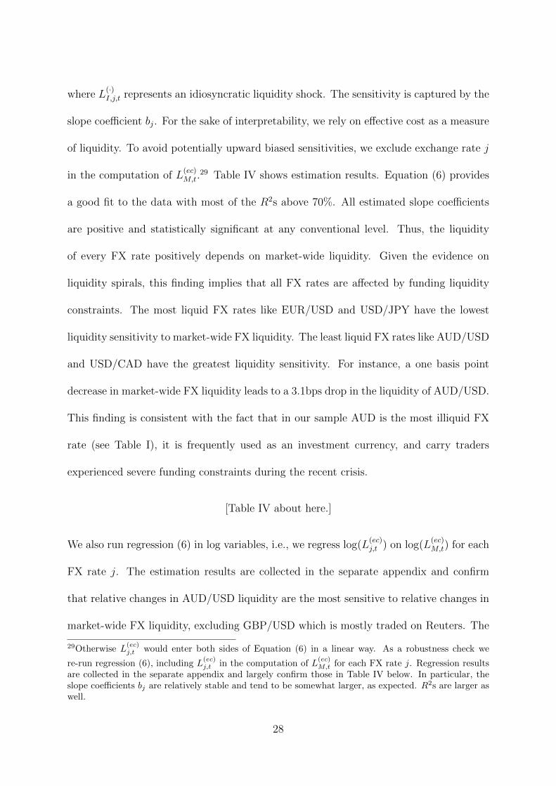
where L(·)I,j,t represents an idiosyncratic liquidity shock. The sensitivity is captured by the
slope coefficient bj. For the sake of interpretability, we rely on effective cost as a measure
of liquidity. To avoid potentially upward biased sensitivities, we exclude exchange rate j
in the computation of L(ec)M,t.
29 Table IV shows estimation results. Equation (6) provides
a good fit to the data with most of the R2s above 70%. All estimated slope coefficients
are positive and statistically significant at any conventional level. Thus, the liquidity
of every FX rate positively depends on market-wide liquidity. Given the evidence on
liquidity spirals, this finding implies that all FX rates are affected by funding liquidity
constraints. The most liquid FX rates like EUR/USD and USD/JPY have the lowest
liquidity sensitivity to market-wide FX liquidity. The least liquid FX rates like AUD/USD
and USD/CAD have the greatest liquidity sensitivity. For instance, a one basis point
decrease in market-wide FX liquidity leads to a 3.1bps drop in the liquidity of AUD/USD.
This finding is consistent with the fact that in our sample AUD is the most illiquid FX
rate (see Table I), it is frequently used as an investment currency, and carry traders
experienced severe funding constraints during the recent crisis.
[Table IV about here.]
We also run regression (6) in log variables, i.e., we regress log(L(ec)j,t ) on log(L
(ec)M,t) for each
FX rate j. The estimation results are collected in the separate appendix and confirm
that relative changes in AUD/USD liquidity are the most sensitive to relative changes in
market-wide FX liquidity, excluding GBP/USD which is mostly traded on Reuters. The
29Otherwise L(ec)j,t would enter both sides of Equation (6) in a linear way. As a robustness check we
re-run regression (6), including L(ec)j,t in the computation of L
(ec)M,t for each FX rate j. Regression results
are collected in the separate appendix and largely confirm those in Table IV below. In particular, theslope coefficients bj are relatively stable and tend to be somewhat larger, as expected. R2s are larger aswell.
28

liquidity of EUR/USD is again the least sensitive.
These findings suggest that managing the liquidity risk of illiquid currencies is partic-
ularly challenging. Not only is the level of liquidity lower, but it is also more sensitive to
changes in market-wide liquidity. In contrast, the most liquid currencies may offer a “liq-
uidity hedge” as they tend to remain relatively liquid, even when market-wide liquidity
drops.
VII. Liquidity Risk Premiums
A. Shocks to Market-wide FX Liquidity
Given the evidence for liquidity spirals and strong declines in market-wide FX liquidity,
the question arises as to whether investors demand a premium for being exposed to liquid-
ity risk. To our knowledge, a theoretical model for currency returns which accommodates
liquidity risk, in the same spirit as, e.g., Lustig, Roussanov, and Verdelhan (2011) has not
yet been developed. However, if liquidity shocks vanish quickly it appears unlikely that
investors would be concerned about liquidity risk. Only long-lasting shocks to market-
wide liquidity are likely to affect investors and require liquidity risk premia (Korajczyk
and Sadka, 2008). This may be the case because investors will probably suffer higher
costs during long and unexpected illiquid environments, and will consequently require a
premium for that risk.30 The separate appendix shows the autocorrelation functions for
the various market-wide FX liquidities. Invariably, all aggregate liquidity proxies exhibit
strong positive autocorrelation, even after several months. Hence a drop in aggregate
30This interpretation may also help to explain why liquidity in equity markets is persistent (Chordia,Roll, and Subrahmanyam (2000, 2001)) and priced (Pastor and Stambaugh, 2003).
29
liquidity is unlikely to be reversed quickly, suggesting that liquidity risk may indeed be
priced.
B. Carry Trade Returns
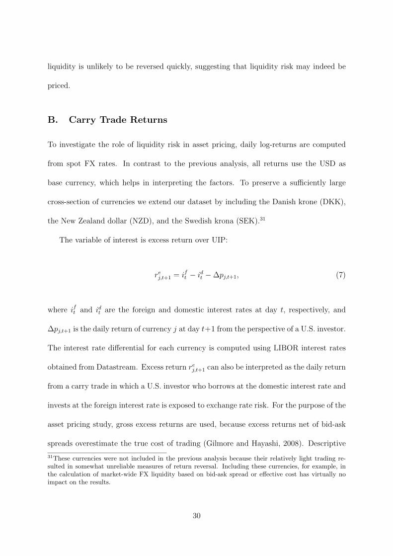
To investigate the role of liquidity risk in asset pricing, daily log-returns are computed
from spot FX rates. In contrast to the previous analysis, all returns use the USD as
base currency, which helps in interpreting the factors. To preserve a sufficiently large
cross-section of currencies we extend our dataset by including the Danish krone (DKK),
the New Zealand dollar (NZD), and the Swedish krona (SEK).31
The variable of interest is excess return over UIP:
rej,t+1 = ift − idt −∆pj,t+1, (7)
where ift and idt are the foreign and domestic interest rates at day t, respectively, and
∆pj,t+1 is the daily return of currency j at day t+1 from the perspective of a U.S. investor.
The interest rate differential for each currency is computed using LIBOR interest rates
obtained from Datastream. Excess return rej,t+1 can also be interpreted as the daily return
from a carry trade in which a U.S. investor who borrows at the domestic interest rate and
invests at the foreign interest rate is exposed to exchange rate risk. For the purpose of the
asset pricing study, gross excess returns are used, because excess returns net of bid-ask
spreads overestimate the true cost of trading (Gilmore and Hayashi, 2008). Descriptive
31These currencies were not included in the previous analysis because their relatively light trading re-sulted in somewhat unreliable measures of return reversal. Including these currencies, for example, inthe calculation of market-wide FX liquidity based on bid-ask spread or effective cost has virtually noimpact on the results.
30
statistics for exchange rate returns, interest rate differentials as well as daily carry trade
returns are depicted in Table V.
[Table V about here.]
Panel (a) shows that the annualized returns of individual exchange rates between
January 2007 and December 2009 are larger in absolute value than those in the longer
sample of Lustig, Roussanov, and Verdelhan (2011). Prior to the bankruptcy of Lehman
Brothers (Panel (b)), the difference in magnitude is rather small. After the collapse (Panel
(c)), larger average and extremely volatile returns occur. Interest rate differentials tend
to be lower in absolute value in the last subsample, mirroring the joint efforts of central
banks to alleviate the economic downturn by lowering interest rates.
Typical low interest rate currencies (JPY, CHF) have a positive excess return over the
whole sample with the appreciation being strongest after September 2008. Immediately
after the Lehman bankruptcy, high interest rate currencies (AUD, NZD) depreciated
strongly, mirroring liquidity spirals and unwinding of carry trades. However, in the
course of 2009, these currencies appreciated against the USD, resulting in a negative
excess return on the USD.32
The crisis led to significant volatility in exchange rates. Standard deviations of carry
trade returns doubled for many currencies when comparing the samples before and after
the Lehman bankruptcy. This large variation and significant carry trade returns require
32A common explanation for this appreciation of high interest rate currencies versus USD is the factthat, at that time, the outlook for the U.S. economy had worsened, in relative terms. Also, the enormousinjection of liquidity into USD (in particular via central bank swap lines) and the Fed’s quantitativeeasing operations probably kept interest rates low in the U.S., thereby weakening the USD. Moreover,investors may have started to set up carry trades again, because the historically low U.S. interest rateshad fueled the search for yields and allowed the USD to be used as a funding currency. Commodityprices increased again in 2009, thus supporting commodity-related currencies such as the AUD.
31
further analysis, which is undertaken below.
C. Liquidity and Carry Trade Returns
Recently, a number of studies have documented comovements in carry trade returns; e.g.,
Lustig, Roussanov, and Verdelhan (2011) and Menkhoff, Sarno, Schmeling, and Schrimpf
(2011). The significant variation and commonality in currency liquidities documented
above suggest that liquidity risk may contribute to this common variation. The sep-
arate appendix reports correlations between carry trade returns and FX liquidity, and
provides evidence for contemporaneous comovements between the two. FX liquidity is
given by liquidity levels, liquidity shocks, and unexpected liquidity shocks. The liquidity
level is the latent market-wide liquidity, as outlined in Section V. As in Pastor and Stam-
baugh (2003) and Acharya and Pedersen (2005), liquidity shocks and unexpected liquidity
shocks are defined as the residuals from an AR(1) model and an AR(2) model fitted to
latent market-wide liquidity, respectively. Typical high interest rate currencies during
our sample period, such as AUD, Canadian dollar (CAD) or NZD, exhibit the largest
positive correlations (with AUD reaching 70% at monthly frequency), meaning that they
depreciate contemporaneously with a decrease in liquidity. Vice versa, JPY, a typical
low interest rate currency, exhibits a negative correlation, meaning that it appreciates
when liquidity drops. Moreover, with the exception of CAD and pound sterling (GBP),
a nearly monotone relation exists between sorting currencies based on decreasing interest
rate differentials (Table V) and increasing liquidity-carry trade return correlations. This
finding is also consistent with liquidity spirals (Table III). The correlation between FX
liquidity and carry trade return is largest in absolute value for shocks at the monthly
32

frequency. Correlations between liquidity shocks and carry trade returns are often twice
the correlations between liquidity levels and returns. Such strong comovements between
carry trade returns and unexpected changes in liquidity are consistent with liquidity risk
being a risk factor for carry trade returns.
D. Liquidity Risk Factor
To formally test whether liquidity risk affects carry trade returns, variation in the cross-
section of returns is assumed to be caused by different exposure to a small number of
risk factors (Ross, 1976). In particular, we introduce a liquidity risk factor given by a
currency portfolio which is long in the two most illiquid and short in the two most liquid
FX rates on each day t. We label this liquidity risk factor IML (illiquid minus liquid).
IML has a natural interpretation as the return in dollars on a zero-cost strategy that
goes long in illiquid currencies and short in liquid currencies.33 As IML is a tradable
risk factor, its computation is straightforward and currency investors can easily hedge
associated liquidity risk exposures. The separate appendix compares IML to a non-
tradable risk factor computed as shocks to latent market-wide liquidity. Both liquidity
factors exhibit similar patterns with a correlation of 0.20 (0.71 for monthly data) and
much larger variation after the bankruptcy of Lehman Brothers.
Lustig, Roussanov, and Verdelhan (2011) introduce a carry trade risk factor, HML,
given by a currency portfolio which is long in high interest rate currencies and short
in low interest rate currencies. They find that HML explains the common variation
in carry trade returns and suggest that this risk factor captures “global risk” for which
33As all FX rates use USD as their base currency, to construct the portfolio IML an investor pays USD2 to buy the two most illiquid currencies and receives USD 2 for selling the two most liquid currencies.
33
carry traders earn a risk premium. Our liquidity risk factor IML is strongly correlated
(0.92) with HML during our sample period. Thus, the risk of liquidity spirals, which is
captured by IML, appears to contribute significantly to “global risk.”
The second risk factor we consider is the “market” risk factor or average excess return,
AER, from Lustig, Roussanov, and Verdelhan (2011):
AERt =1
N
N∑j=1
rej,t, (8)
which is the average return for a U.S. investor who goes long in all N exchange rates
available in the sample. AER has also a natural interpretation as the currency “market”
return in USD available to a U.S. investor and is driven by the fluctuations of the USD
against a broad basket of currencies. As shown in the separate appendix this level risk
factor does not exhibit significant variation compared to both IML and HML.
We now estimate a factor model to assess the relative importance and cross-sectional
differences in exposure to the risk factors IML and AER. The following asset pricing
model is estimated on a daily basis for each FX rate j:
rej,t = αj + βAER,jAERt + βIML,jIMLt + εj,t, (9)
where βAER,j and βIML,j denote the exposure of the carry trade return j to the market
risk factor and liquidity risk factor, respectively. Any unusual or abnormal return that
is not explained by the FX risk factors is captured by the constant αj. The regression
results are shown in Table VI.
[Table VI about here.]
34
Equation (9) provides a good fit to the data with adjusted-R2s ranging from approxi-
mately 60% to 90%. Thus, the vast majority of variation in carry trade returns can be
explained by exposure to two risk factors. Moreover, no currency pair exhibits a signif-
icant αj, indicating that the pricing model appropriately captures the characteristics of
carry trade returns. Liquidity betas, βIML,j, are economically and statistically significant
at any conventional level. For example, when our liquidity factor decreases by one stan-
dard deviation, AUD depreciates by 0.53 standard deviations, whereas JPY appreciates
by 0.98 standard deviations.34 Unreported results show that adjusted-R2s attain 60%
when only IML is included as regressor, highlighting the crucial role of liquidity risk. In
line with Lustig, Roussanov, and Verdelhan (2011), all exchange rates load fairly equally
on the market risk factor, which therefore helps to explain the average level of carry trade
returns. In contrast, liquidity betas, βIML,j, vary significantly across exchange rates.35
An interesting pattern emerges from Table VI. Typical high interest rate currencies,
such as AUD or NZD, exhibit the largest positive liquidity betas, thus providing exposure
to liquidity risk. Vice versa, low interest rate currencies, such as JPY or CHF, exhibit
the largest negative liquidity betas, thus offering insurance against liquidity risk. To
help visualize the relation between liquidity betas and interest rate differentials, Figure 5
shows the corresponding scatter plot.
[Figure 5 about here.]
When FX liquidity improves, high interest rate currencies appreciate further, because
34These findings are not driven by the events after the bankruptcy of Lehman Brothers. When onlyconsidering the period before the bankruptcy the number of standard deviations for AUD and JPY are0.51 and 0.86, respectively. The separate appendix collects these results for all currencies in our sample.35Unreported regression results show that estimates of βIML,j remain largely the same when addingHML as a regressor in Equation (9), although standard errors are obviously unreliable due to collinearitybetween IML and HML.
35
of positive liquidity betas, while low interest rate currencies depreciate further, because
of negative liquidity betas, increasing the deviation of FX rates from UIP. During an
unwinding of carry trades (i.e., when high interest currencies are sold and low interest
rate currencies are bought), because of liquidity spirals, market-wide FX liquidity drops,
inducing a higher price impact of trades. Because FX liquidity falls and liquidity betas
have opposite signs, high interest rate currencies depreciate further and low interest rate
currencies appreciate further, exacerbating currency crashes and inflicting large losses on
carry traders.
Figure 6 illustrates this phenomenon for the AUD-JPY carry trade. Cumulative
returns of one U.S. dollar invested in AUD/USD and JPY/USD carry trades are depicted
along with market-wide FX liquidity. The Australian dollar has a positive liquidity
beta (0.33) and the cumulative AUD/USD carry trade return tends to comove with
market-wide FX liquidity. In contrast, JPY has a negative liquidity beta (−0.38) and the
cumulative JPY/USD carry trade return tends to mirror FX liquidity fluctuations. The
unwinding of carry trades on August 16, 2007 results in a drop in the FX liquidity and
sharp movements in AUD and JPY in opposite directions. Similar opposite movements
are evident around the Lehman bankruptcy.
[Figure 6 about here.]
Liquidity betas reflect the liquidity features of the various currencies. High inter-
est rate currencies tend to have low liquidity (Table I) and high liquidity sensitivity to
fluctuations in market-wide FX liquidity (Table IV). Such low liquidity features appear
to command a liquidity risk premium which is reflected in large positive liquidity betas
(Table VI). Vice versa, low interest rate currencies tend to have higher liquidity and
36
less liquidity sensitivity to market-wide FX liquidity. Such high liquidity features are re-
flected in negative liquidity betas and thus lower returns when market-wide FX liquidity
improves. Such lower returns are the “insurance premiums” for holding currencies which
will tend to deliver higher returns in bad times, i.e., when FX liquidity drops.
Finally, the trigger of this mechanism appears to be a liquidity spiral. As shown
in Section VI, when traders’ funding liquidity deteriorates, market-wide FX liquidity
drops (Table III) with an impact on currency returns which is diametrically opposite,
depending on the sign of their liquidity betas. Consistent with this interpretation, highly
liquid currencies, the liquidity of which is least sensitive to market-wide liquidity, and
which are usually not involved in carry trades, such as the euro (EUR), have a liquidity
beta close to zero.
The separate appendix presents four robustness checks that confirm our results. First,
in the same spirit as Lustig, Roussanov, and Verdelhan (2011), we regress FX rate returns,
−∆pj,t+1, rather than carry trade returns, rej,t+1, on liquidity and market risk factors. All
liquidity betas are virtually the same as in Table VI. This implies that low interest rate
currencies offer insurance against liquidity risk because they appreciate when market-
wide FX liquidity drops, not because the interest rates on these currencies increase.
On the other hand, high interest rate currencies expose carry traders to liquidity risk
because they depreciate when FX liquidity drops, not because the interest rates on those
currencies decline. Second, we add the interest rate differential, idt − ift , as an explanatory
variable when regressing FX rate returns on liquidity and market risk factors. Model (9)
is a special case of the latter when the slope of idt − ift is restricted to be one. Again, all
liquidity betas are almost unchanged. Third, in Equation (9) we replace IML by latent
37
unexpected shocks to market-wide FX liquidity. The new liquidity betas largely share
the same pattern as liquidity betas in Table VI. Fourth, we use Equation (9) to explain
carry trade index returns, namely the returns of the Deutsche Bank’s “G10 Currency
Harvest” (DBV) exchange traded fund.36 The liquidity beta for DBV is significant at
any conventional level and very close to the liquidity beta for AUD. The corresponding
intercept is not statistically different from zero. This finding confirms the key role of
liquidity risk in explaining carry trade returns.
All in all, our findings suggest that liquidity risk is an important risk factor for FX
returns. The presence of this factor is consistent with the theory of liquidity spirals and
currency crashes. Investors are exposed to these spirals and will thus demand a risk
premium as compensation for bearing liquidity risk. It remains to be investigated, with
a longer sample, whether liquidity risk is also priced in the cross-section of carry trade
returns and during other periods. There are at least two reasons to expect that this will be
the case. First, as mentioned above, our liquidity risk factor is strongly correlated (0.92)
with the carry trade factor of Lustig, Roussanov, and Verdelhan (2011), which is shown to
have a large impact on monthly carry trade returns from 1983 to 2008. Second, recently
Banti, Phylaktis, and Sarno (2011) followed our work and studied the risk premium of
FX liquidity. Although they consider only the return reversal aspect of liquidity and use
data from custodian banks,37 they provide some evidence of liquidity risk being priced in
currency portfolios.
36We thank an anonymous referee for suggesting this robustness check.37The separate appendix compares our EBS dataset to data from custodian banks. Besides dataset andliquidity measures there are other important differences between the two studies related to identificationof liquidity risk, analysis of commonality, and inference procedure.
38
VIII. Conclusion
Using a novel and comprehensive dataset of intraday data, this paper provides the first
systematic study of liquidity in the foreign exchange market. Contrary to common per-
ceptions of the FX market being highly liquid at all times, we find significant cross-
sectional and temporal variation in liquidities, substantial costs due to FX illiquidity for
carry traders, and ample evidence of commonality in liquidities, i.e., strong comovements
across the liquidity of different currencies. Such commonality implies that FX liquidity
is largely driven by shocks that affect the FX market as whole rather than individual FX
rates. It also implies that the FX market is likely to become illiquid precisely when the
U.S. equity and bond markets are illiquid - given the large liquidity comovements across
markets that we document - impairing the efficacy of international and cross asset class
diversification as a means of reducing liquidity risk.
Second, we analyze the impact of liquidity risk on carry trades. Low interest rate cur-
rencies tend to have high liquidity, low liquidity sensitivities to market-wide FX liquidity,
and negative liquidity betas, thus offering insurance against liquidity risk. The opposite
is true for high interest rate currencies which provide exposure to liquidity risk. Negative
liquidity betas reflect an “insurance premium” for relatively high liquidity features of low
interest rate currencies. Positive liquidity betas reflect compensation for relatively low
liquidity features of high interest rate currencies. These liquidity features and liquidity
betas rationalize the impact of market-wide FX liquidity on carry trade returns. When
FX liquidity improves, high interest rate currencies tend to appreciate, because of positive
liquidity betas, while low interest rate currencies tend to depreciate, due to their negative
liquidity betas, increasing the deviation of FX rates from UIP. During the unwinding of
39

carry trades, because of liquidity spirals, market-wide FX liquidity drops and the price
impact of trades increases. As FX liquidity falls and liquidity betas have opposite signs,
high interest rate currencies tend to depreciate and low interest rate currencies tend to
appreciate, exacerbating currency crashes.
To compute liquidity betas we introduce a novel tradable liquidity risk factor which
is shown to have a strong impact on carry trade returns during our sample period from
January 2007 to December 2009. This suggests that liquidity risk is priced in currency
returns. Finally, we provide evidence that liquidity spirals may trigger the mechanisms
above. When traders’ funding liquidity decreases, market-wide FX liquidity drops (a
cross-market effect), impacting currency returns via their liquidity betas.
Several policy implications can be drawn from this study. From a central bank per-
spective, an implication of FX liquidity commonality is that providing liquidity for a
specific FX rate may have positive spillover effects to other currencies as well. Take the
example of high interest rate currencies during an unwinding of carry trade. A central
bank’s liquidity injection in its own currency could alleviate liquidity strains in other
“investment” currencies and moderate the sudden appreciation (depreciation) of other
“borrowing” (“investment”) currencies. Our empirical evidence on liquidity spirals also
appears insightful. To use the same example, monetary policies aimed at relieving fund-
ing market constraints could also improve FX market liquidity in all exchange rates. But
abundant liquidity may have adverse consequences. Overwhelming liquidity in one cur-
rency tends to spread to other currencies and even more so to “investment” currencies. In
risk-taking environments with attractive carry trade opportunities, ample liquidity could
bolster speculative trading.
40
The use of EBS intraday data limits the extension of our sample. It remains to
be investigated whether liquidity risk plays an important role in explaining carry trade
returns in other periods as well. In fact, our liquidity risk factor turns out to be highly
correlated with another carry trade risk factor which is shown to have a large impact on
carry trade returns over decades. Investigating the impact of liquidity risk on carry trade
returns during other periods appears to be a promising direction for future research.
41
References
Acharya, V. V., and L. H. Pedersen, 2005, “Asset Pricing with Liquidity Risk,” Journal
of Financial Economics, 77, 375–410.
Aıt-Sahalia, Y., P. A. Mykland, and L. Zhang, 2005, “How Often to Sample a Continuous-
Time Process in the Presence of Market Microstructure Noise,” Review of Financial
Studies, 18, 351–416.
Amihud, Y., 2002, “Illiquidity and Stock Returns: Cross-Section and Time-Series Ef-
fects,” Journal of Financial Markets, 5, 31–56.
Amihud, Y., and H. Mendelson, 1986, “Asset Pricing and the Bid-Ask Spread,” Journal
of Financial Economics, 17, 223–249.
Bacchetta, P., and E. van Wincoop, 2010, “Infrequent Portfolio Decisions: A Solution to
the Forward Discount Puzzle,” American Economic Review, 100, 837–869.
Backus, D., S. Foresi, and C. Telmer, 2001, “Affine Term Structure Models and the
Forward Premium Anomaly,” Journal of Finance, 56, 279–304.
Bank for International Settlements, 2010, “Foreign Exchange and Derivatives Market
Activity in April 2010,” Triennial Central Bank Survey.
Banti, C., K. Phylaktis, and L. Sarno, 2011, “Liquidity in the Foreign Exchange Market,”
Working paper, Cass Business School.
Bao, J., J. Pan, and J. Wang, 2011, “The Illiquidity of Corporate Bonds,” Journal of
Finance, forthcoming.
Bekaert, G., 1996, “The Time Variation of Risk and Return in Foreign Exchange Markets:
A General Equilibrium Perspective,” Review of Financial Studies, 9, 427–470.
Bekaert, G., C. R. Harvey, and C. Lundblad, 2007, “Liquidity and Expected Returns:
Lessons from Emerging Markets,” Review of Financial Studies, 20, 1783–1832.
Bekaert, G., and R. Hodrick, 1992, “Characterizing Predictable Components in Excess
Returns on Equity and Foreign Exchange Markets,” Journal of Finance, 47, 467–509.
Berger, D. W., A. P. Chaboud, S. V. Chernenko, E. Howorka, and J. H. Wright, 2008,
“Order Flow and Exchange Rate Dynamics in Electronic Brokerage System Data,”
Journal of International Economics, 75, 93–109.
42

Breedon, F., and P. Vitale, 2010, “An Empirical Study of Portfolio-Balance and Informa-
tion Effects of Order Flow on Exchange Rates,” Journal of International Money and
Finance, 29, 504–524.
Brennan, M., and Y. Xia, 2006, “International Capital Markets and Foreign Exchange
Risk,” Review of Financial Studies, 19, 753–795.
Brunnermeier, M. K., S. Nagel, and L. H. Pedersen, 2009, “Carry Trades and Currency
Crashes,” NBER Macroeconomics Annual 2008, 23, 313–347.
Brunnermeier, M. K., and L. H. Pedersen, 2005, “Predatory Trading,” Journal of Fi-
nance, 60, 1825–1863.
, 2009, “Market Liquidity and Fund Liquidity,” Review of Financial Studies, 22,
2201–2238.
Burnside, C., 2009, “Carry Trades and Currency Crashes: A Comment,” NBER Macroe-
conomics Annual 2008.
Burnside, C., M. Eichenbaum, I. Kleshchelski, and S. Rebelo, 2011, “Do Peso Problems
Explain the Returns to the Carry Trade?,” Review of Financial Studies, 24, 853–891.
Campbell, J. Y., S. J. Grossman, and J. Wang, 1993, “Trading Volume and Serial Cor-
relation in Stock Returns,” Quarterly Journal of Economics, 108, 905–939.
Campbell, J. Y., K. Serfaty-de Medeiros, and L. M. Viceira, 2010, “Global Currency
Hedging,” Journal of Finance, 65, 87–121.
Campello, M., E. Giambona, J. R. Graham, and C. R. Harvey, 2011, “Liquidity Man-
agement and Corporate Investment During a Financial Crisis,” Review of Financial
Studies, forthcoming.
Chaboud, A. P., S. V. Chernenko, and J. H. Wright, 2007, “Trading Activity and Ex-
change Rates in High-Frequency EBS Data,” International Finance Discussion Papers
903, Board of Governors of the Federal Reserve System and Harvard University.
Chordia, T., R. Roll, and A. Subrahmanyam, 2000, “Commonality in Liquidity,” Journal
of Financial Economics, 56, 3–28.
, 2001, “Market Liquidity and Trading Activity,” Journal of Finance, 56, 501–530.
Chordia, T., A. Sarkar, and A. Subrahmanyam, 2005, “An Empirical Analysis of Stock
and Bond Market Liquidity,” Review of Financial Studies, 18, 85–130.
43
Dick-Nielsen, J., P. Feldhutter, and D. Lando, 2011, “Corporate Bond Liquidity Before
and After the Onset of the Subprime Crisis,” Journal of Financial Economics, forth-
coming.
Evans, M. D. D., and R. K. Lyons, 2002, “Order Flow and Exchange Rate Dynamics,”
Journal of Political Economy, 110, 170–180.
Fama, E. F., 1984, “Forward and Spot Exchange Rates,” Journal of Monetary Economics,
14, 319–338.
Fama, E. F., and K. R. French, 1993, “Common Risk Factors in the Returns on Stocks
and Bonds,” Journal of Financial Economics, 33, 3–56.
Farhi, E., S. P. Fraiberger, X. Gabaix, R. Ranciere, and A. Verdelhan, 2009, “Crash Risk
in Currency Markets,” NBER Working paper 15062, Harvard University, New York
University, International Monetary Fund, and Boston University.
Farhi, E., and X. Gabaix, 2011, “Rare Disasters and Exchange Rates: A Theory of the
Forward Premium Puzzle,” Working paper, Harvard University, New York University.
Fleming, M., and E. Remolona, 1999, “Price Formation and Liquidity in the U.S. Treasury
Market: The Response to Public Informaion,” Journal of Finance, 54, 1901–1915.
Foucault, T., O. Kadan, and E. Kandel, 2005, “Limit Order Book as a Market for Liq-
uidity,” Review of Financial Studies, 18, 1171–1217.
Froot, K., and R. Thaler, 1990, “Anomalies: Foreign Exchange,” Journal of Economic
Perspectives, 4, 179–192.
Gilmore, S., and F. Hayashi, 2008, “Emerging Market Currency Excess Returns,” NBER
Working paper 14528, AIG Financial Products and University of Tokyo.
Glen, J., and P. Jorion, 1993, “Currency Hedging for International Portfolios,” Journal
of Finance, 48, 1865–1886.
Goyenko, R. Y., C. W. Holden, and C. A. Trzcinka, 2009, “Do Liquidity Measures Mea-
sure Liquidity?,” Journal of Financial Economics, 92, 153–181.
Green, R., D. Li, and N. Schuerhoff, 2010, “Price Discovery in Illiquid Markets: Do
Financial Asset Prices Rise Faster Than They Fall?,” Journal of Finance, 65, 1669–
1702.
Hansen, L. P., and R. J. Hodrick, 1980, “Forward Exchange Rates as Optimal Predictors
of Future Spot Rates: An Econometric Analysis,” Journal of Political Economy, 88,
829–853.
44
Harvey, C. R., B. Solnik, and G. Zhou, 2002, “What Determines Expected International
Asset Returns?,” Annals of Economics and Finance, 3, 249–298.
Hasbrouck, J., 2009, “Trading Costs and Returns for US Equities: Estimating Effective
Costs from Daily Data,” Journal of Finance, 64, 1445–1477.
Hasbrouck, J., and D. Seppi, 2001, “Common Factors in Prices, Order Flows, and Liq-
uidity,” Journal of Financial Economics, 59, 383–411.
Hodrick, R., and S. Srivastava, 1986, “The Covariation of Risk Premiums and Expected
Future Spot Rates,” Journal of International Money and Finance, 3, 5–30.
Holden, C. W., 2009, “New Low-Frequency Spread Measures,” Journal of Financial Mar-
kets, 12, 778–813.
Jones, C. M., G. Kaul, and M. L. Lipson, 1994, “Transactions, Volume, and Volatility,”
Review of Financial Studies, 7, 631–651.
Jurek, J. W., 2009, “Crash-Neutral Currency Carry Trades,” Working paper, Princeton
University.
Korajczyk, R. A., and R. Sadka, 2008, “Pricing the Commonality Accross Alternative
Measures of Liquidity,” Journal of Financial Economics, 87, 45–72.
Kyle, A., 1985, “Continuous Auctions and Insider Trading,” Econometrica, 53, 1315–
1335.
Lee, C., and M. Ready, 1991, “Inferring Trade Direction from Intraday Data,” Journal
of Finance, 46, 733–746.
Lustig, H. N., N. L. Roussanov, and A. Verdelhan, 2011, “Common Risk Factors in
Currency Markets,” Review of Financial Studies, forthcoming.
Lustig, H. N., and A. Verdelhan, 2007, “The Cross-Section of Foreign Currency Risk
Premia and Consumption Growth Risk,” American Economic Review, 97, 89–117.
Lyons, R. K., 2001, The Microstructure Approach to Exchange Rates. MIT Press.
Marsh, I. W., and C. O’Rourke, 2005, “Customer Order Flow and Exchange Rate Move-
ments: Is there Really Information Content?,” Working paper, Cass Business School.
Melvin, M., and M. P. Taylor, 2009, “The Crisis in the Foreign Exchange Market,”
Journal of International Money and Finance, 28, 1317–1330.
45

Menkhoff, L., L. Sarno, M. Schmeling, and A. Schrimpf, 2011, “Carry Trades and Global
Foreign Exchange Volatility,” Journal of Finance, forthcoming.
Morris, S., and H. S. Shin, 2004, “Liquidity Black Holes,” Review of Finance, 8, 1–18.
Pastor, L., and R. F. Stambaugh, 2003, “Liquidity Risk and Expected Stock Returns,”
Journal of Political Economy, 111, 642–685.
Plantin, G., and H. S. Shin, 2011, “Carry Trades, Monetary Policy and Speculative
Dynamics,” Working paper, London Business School and Princeton University.
Ranaldo, A., and P. Soderlind, 2010, “Safe Haven Currencies,” Review of Finance, 14,
385–407.
Roll, R., 1984, “A Simple Implicit Measure of the Effective Bid-Ask Spread in an Efficient
Market,” Journal of Finance, 39, 1127–1139.
Ross, S. A., 1976, “The Arbitrage Theory of Capital Asset Pricing,” Journal of Economic
Theory, 13, 341–360.
Rosu, I., 2009, “A Dynamic Model of the Limit Order Book,” Review of Financial Studies,
22, 4601–4641.
Sadka, R., 2006, “Momentum and Post-earnings Announcement Drift Anomalies,” Jour-
nal of Financial Economics, 80, 309–349.
Shleifer, A., and R. Vishny, 1997, “The Limits of Arbitrage,” Journal of Finance, 52,
35–55.
Stoll, H. R., 1978, “The Supply of Dealer Services in Securities Markets,” Journal of
Finance, 33, 1133–1151.
Verdelhan, A., 2010, “A Habit-Based Explanation of the Exchange Rate Risk Premium,”
Journal of Finance, 65, 123–145.
World Federation of Exchanges, 2009, 2009 Annual Report and Statistics. Paris, France.
Zhang, L., P. A. Mykland, and Y. Aıt-Sahalia, 2005, “A Tale of Two Time Scales:
Determining Integrated Volatility With Noisy High-Frequency Data,” Journal of the
American Statistical Association, 100, 1394–1411.
46
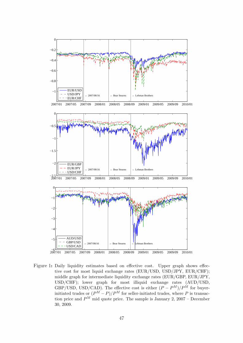
2007/01 2007/05 2007/09 2008/01 2008/05 2008/09 2009/01 2009/05 2009/09 2010/01
−1
−0.8
−0.6
−0.4
−0.2
0
← Lehman Brothers← Bear Stearns← 2007/08/16
EUR/USDUSD/JPYEUR/CHF
2007/01 2007/05 2007/09 2008/01 2008/05 2008/09 2009/01 2009/05 2009/09 2010/01−2.5
−2
−1.5
−1
−0.5
0
← Lehman Brothers← Bear Stearns← 2007/08/16
EUR/GBPEUR/JPYUSD/CHF
2007/01 2007/05 2007/09 2008/01 2008/05 2008/09 2009/01 2009/05 2009/09 2010/01−6
−5
−4
−3
−2
−1
0
← Lehman Brothers← Bear Stearns← 2007/08/16
AUD/USDGBP/USDUSD/CAD
Figure 1: Daily liquidity estimates based on effective cost. Upper graph shows effec-tive cost for most liquid exchange rates (EUR/USD, USD/JPY, EUR/CHF);middle graph for intermediate liquidity exchange rates (EUR/GBP, EUR/JPY,USD/CHF); lower graph for most illiquid exchange rates (AUD/USD,GBP/USD, USD/CAD). The effective cost is either (P − PM )/PM for buyer-initiated trades or (PM −P )/PM for seller-initiated trades, where P is transac-tion price and PM mid quote price. The sample is January 2, 2007 – December30, 2009.
47
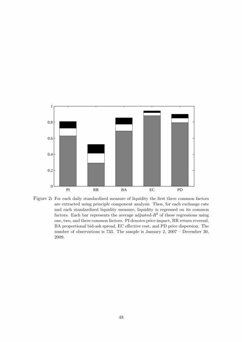
PI RR BA EC PD0
0.2
0.4
0.6
0.8
1
Figure 2: For each daily standardized measure of liquidity the first three common factorsare extracted using principle component analysis. Then, for each exchange rateand each standardized liquidity measure, liquidity is regressed on its commonfactors. Each bar represents the average adjusted-R2 of these regressions usingone, two, and three common factors. PI denotes price impact, RR return reversal,BA proportional bid-ask spread, EC effective cost, and PD price dispersion. Thenumber of observations is 733. The sample is January 2, 2007 – December 30,2009.
48

2007/01 2007/05 2007/09 2008/01 2008/05 2008/09 2009/01 2009/05 2009/09 2010/01−80
−60
−40
−20
0
20
← Lehman Brothers← Bear Stearns← 2007/08/16
FX liq.VIXTED
Figure 3: Latent market-wide FX liquidity (Equation (5)), the negative of the ChicagoBoard Options Exchange Volatility Index (VIX) as well as the negative of theTED spread. The sample is January 2, 2007 – December 30, 2009.
49
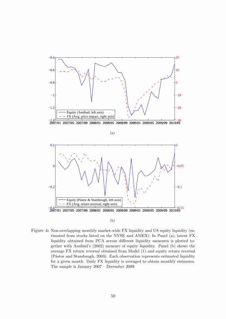
2007/01 2007/05 2007/09 2008/01 2008/05 2008/09 2009/01 2009/05 2009/09 2010/01−1.4
−1.2
−1
−0.8
−0.6
−0.4
2007/01 2007/05 2007/09 2008/01 2008/05 2008/09 2009/01 2009/05 2009/09 2010/01−30
−20
−10
0
10
20
Equity (Amihud, left axis)FX (Avg. price impact, right axis)
(a)
2007/01 2007/05 2007/09 2008/01 2008/05 2008/09 2009/01 2009/05 2009/09 2010/01−0.4
−0.2
0
0.2
2007/01 2007/05 2007/09 2008/01 2008/05 2008/09 2009/01 2009/05 2009/09 2010/01−0.15
−0.1
−0.05
0
Equity (Pástor & Stambough, left axis)FX (Avg. return reversal, right axis)
(b)
Figure 4: Non-overlapping monthly market-wide FX liquidity and US equity liquidity (es-timated from stocks listed on the NYSE and AMEX). In Panel (a), latent FXliquidity obtained from PCA across different liquidity measures is plotted to-gether with Amihud’s (2002) measure of equity liquidity. Panel (b) shows theaverage FX return reversal obtained from Model (1) and equity return reversal(Pastor and Stambaugh, 2003). Each observation represents estimated liquidityfor a given month. Daily FX liquidity is averaged to obtain monthly estimates.The sample is January 2007 – December 2009.
50
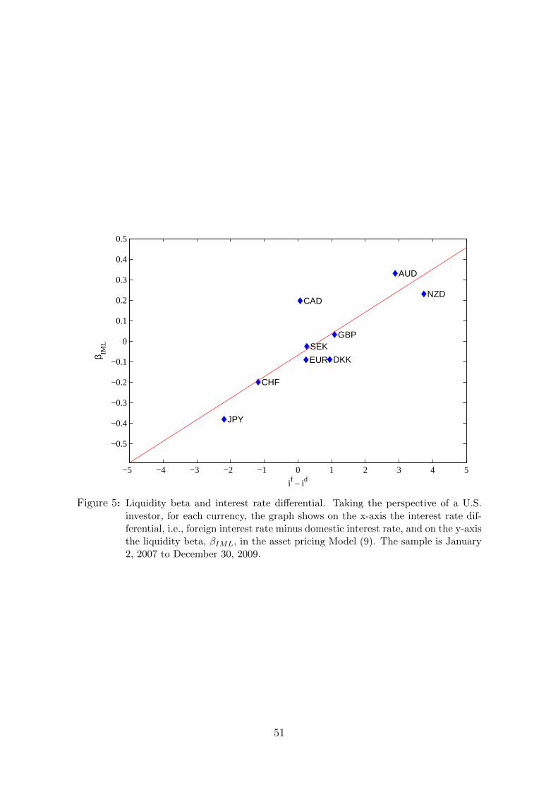
−5 −4 −3 −2 −1 0 1 2 3 4 5
−0.5
−0.4
−0.3
−0.2
−0.1
0
0.1
0.2
0.3
0.4
0.5
if – id
β IML
AUD
CAD
DKKEUR
JPY
NZD
SEK
CHF
GBP
Figure 5: Liquidity beta and interest rate differential. Taking the perspective of a U.S.investor, for each currency, the graph shows on the x-axis the interest rate dif-ferential, i.e., foreign interest rate minus domestic interest rate, and on the y-axisthe liquidity beta, βIML, in the asset pricing Model (9). The sample is January2, 2007 to December 30, 2009.
51
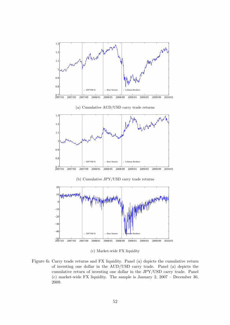
2007/01 2007/05 2007/09 2008/01 2008/05 2008/09 2009/01 2009/05 2009/09 2010/010.7
0.8
0.9
1
1.1
1.2
1.3
← Lehman Brothers← Bear Stearns← 2007/08/16
(a) Cumulative AUD/USD carry trade returns
2007/01 2007/05 2007/09 2008/01 2008/05 2008/09 2009/01 2009/05 2009/09 2010/010.7
0.8
0.9
1
1.1
1.2
1.3
← Lehman Brothers← Bear Stearns← 2007/08/16
(b) Cumulative JPY/USD carry trade returns
2007/01 2007/05 2007/09 2008/01 2008/05 2008/09 2009/01 2009/05 2009/09 2010/01−50
−40
−30
−20
−10
0
10
20
← Lehman Brothers← Bear Stearns← 2007/08/16
(c) Market-wide FX liquidity
Figure 6: Carry trade returns and FX liquidity. Panel (a) depicts the cumulative returnof investing one dollar in the AUD/USD carry trade. Panel (a) depicts thecumulative return of investing one dollar in the JPY/USD carry trade. Panel(c) market-wide FX liquidity. The sample is January 2, 2007 – December 30,2009.
52

Tab
leI:
Dai
lyli
qu
idit
ym
easu
res
AU
D/U
SD
EU
R/C
HF
EU
R/G
BP
EU
R/JP
YE
UR
/U
SD
GB
P/U
SD
US
D/C
AD
US
D/C
HF
US
D/JP
Y
Pri
ceim
pact
Mea
n1.
060.
120.
500.2
60.0
70.4
30.8
40.1
80.1
1
Std
.d
ev.
0.77
0.07
0.29
0.1
50.0
80.3
10.4
70.0
80.0
5
Ret
urn
rever
sal
(nu
mb
erof
lagged
ord
erfl
owK
=5)
Mea
n−
0.17
−0.
03−
0.09
−0.0
5−
0.0
1−
0.1
0−
0.1
6−
0.0
3−
0.0
2
Std
.d
ev.
0.32
0.03
0.14
0.0
50.0
10.1
30.2
60.0
40.0
2
Bid
-ask
spre
ad
(in
bp
s)
Mea
n5.
752.
074.
752.2
11.0
56.1
68.2
72.5
01.5
0
Std
.d
ev.
3.87
1.03
2.96
0.9
60.2
97.4
47.6
31.1
10.4
1
Eff
ecti
veco
st(i
nb
ps)
Mea
n1.
380.
360.
810.4
30.3
10.8
11.2
60.4
50.4
2
Std
.d
ev.
0.78
0.11
0.33
0.1
70.0
60.4
80.4
60.1
10.1
0
Volu
me
wei
ghte
deff
ecti
veco
st(i
nb
ps)
Mea
n1.
110.
280.
710.3
30.2
10.6
61.0
70.3
40.2
7
Std
.d
ev.
0.64
0.10
0.30
0.1
40.0
40.4
10.4
10.1
00.0
7
Pri
ced
isp
ersi
on
(TS
RV
,five
min
ute
s,in
%,
an
nu
aliz
ed)
Mea
n14
.25
5.36
8.28
12.2
68.9
111.3
111.8
49.8
110.4
1
Std
.d
ev.
9.59
3.21
4.36
7.3
94.4
28.2
95.3
84.1
44.8
4
Notes:
Th
ista
ble
show
ssu
mm
ary
stat
isti
csfo
rva
riou
sd
ail
ym
easu
res
of
liqu
idit
y.P
rice
imp
act
isth
ero
bust
lyes
tim
ate
dco
effici
ent
ofco
nte
mp
oran
eou
sor
der
flow
,ϕt,
ina
regre
ssio
nof
on
e-m
inu
tere
turn
son
conte
mp
ora
neo
us
an
dla
gged
ord
erfl
ow(E
qu
atio
n(1
)).
Ret
urn
rever
sal
isth
esu
mof
the
coeffi
cien
tsof
lagged
ord
erfl
ow,∑ K k
=1γt,k,
inth
esa
me
regre
ssio
n.
Bid
-ask
spre
add
enot
esth
eav
erag
ep
rop
ort
ion
al
bid
-ask
spre
ad
com
pu
ted
usi
ng
intr
ad
ayd
ata
for
each
trad
ing
day
.E
ffec
tive
cost
isth
eav
erag
ed
iffer
ence
bet
wee
nth
etr
an
sact
ion
pri
cean
dth
eb
id/ask
qu
ote
pre
vail
ing
at
the
tim
eof
the
trad
e.P
rice
dis
per
sion
for
each
trad
ing
day
ises
tim
ate
du
sin
gtw
o-s
cale
reali
zed
vola
tili
ty(T
SR
V).
Itis
exp
ress
edin
per
centa
geon
anan
nu
alb
asis
.T
he
sam
ple
isJanu
ary
2,
2007
–D
ecem
ber
30,
2009.
53

Tab
leII:
Cor
rela
tion
bet
wee
nli
qu
idit
yof
diff
eren
tas
set
clas
ses
FX
Equ
ity
Bon
d
Ave
rage
PC
A
RR
PI
BA
EC
PD
LL
PS
AM
CO
10y
FX
avg.
ret.
reve
rsal
1
pri
ceim
pac
t0.8
95
1
bid
-ask
spre
ad0.
853
0.8
90
1
effec
tive
cost
0.8
95
0.8
97
0.9
54
1
pri
ced
isp
ersi
on0.8
60
0.9
00
0.9
49
0.9
46
1
FX
PC
Ala
tent
liqu
idit
y0.9
27
0.9
55
0.9
53
0.9
23
0.9
38
1
Equ
ity
Pas
tor/
Sta
mb
augh
0.2
74
0.3
99
0.3
00
0.2
82
0.3
77
0.3
37
1
Am
ihu
d0.
672
0.6
39
0.6
45
0.6
40
0.7
21
0.6
77
0.3
56
1
Bon
dC
orp
orat
e0.9
09
0.8
83
0.9
16
0.9
09
0.9
22
0.9
29
0.4
01
0.7
25
1
10y
Tre
asu
ry0.8
69
0.7
98
0.8
63
0.8
80
0.8
79
0.8
41
0.2
19
0.6
73
0.9
31
1
Notes:
Cor
rela
tion
sb
etw
een
mar
ket-
wid
eliqu
idit
ym
easu
res
for
the
FX
mar
ket
(ret
urn
reve
rsal;
pri
ceim
pac
t;b
id-a
sksp
read
;eff
ecti
veco
st;
pri
ced
isp
ersi
on
;la
tent
liqu
idit
y),
for
the
equ
ity
mark
et(P
asto
r/S
tam
bau
gh;
Am
ihu
d),
for
the
corp
ora
teb
on
dm
ark
et(C
orp
ora
te),
an
dfo
rth
eU
.S.
10-y
ear
Tre
asu
ryb
ond
mar
ket
(10y
Tre
asu
ry).
Corr
elati
on
sare
com
pu
ted
usi
ng
36
non-o
verl
ap
pin
gm
onth
lyob
serv
atio
ns.
Th
esa
mp
leis
Janu
ary
2007
–D
ecem
ber
2009.
54
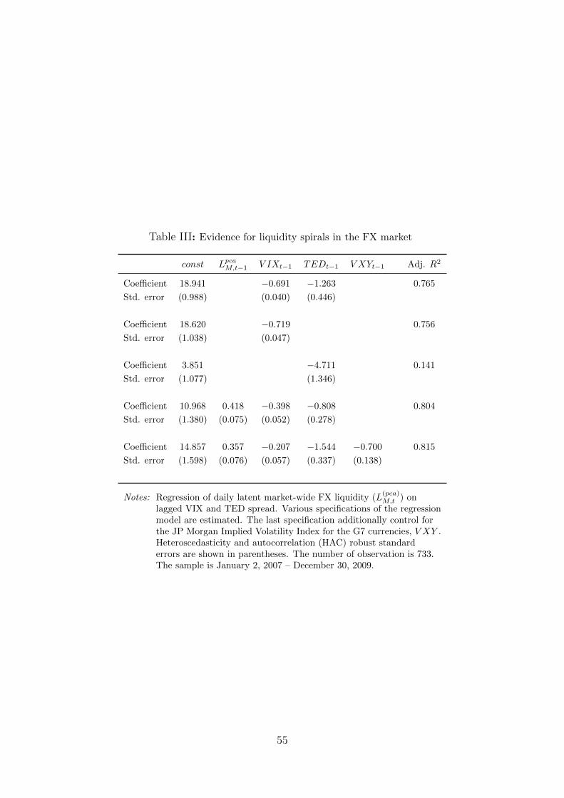
Table III: Evidence for liquidity spirals in the FX market
const LpcaM,t−1 V IXt−1 TEDt−1 V XYt−1 Adj. R2
Coefficient 18.941 −0.691 −1.263 0.765
Std. error (0.988) (0.040) (0.446)
Coefficient 18.620 −0.719 0.756
Std. error (1.038) (0.047)
Coefficient 3.851 −4.711 0.141
Std. error (1.077) (1.346)
Coefficient 10.968 0.418 −0.398 −0.808 0.804
Std. error (1.380) (0.075) (0.052) (0.278)
Coefficient 14.857 0.357 −0.207 −1.544 −0.700 0.815
Std. error (1.598) (0.076) (0.057) (0.337) (0.138)
Notes: Regression of daily latent market-wide FX liquidity (L(pca)M,t ) on
lagged VIX and TED spread. Various specifications of the regressionmodel are estimated. The last specification additionally control forthe JP Morgan Implied Volatility Index for the G7 currencies, V XY .Heteroscedasticity and autocorrelation (HAC) robust standarderrors are shown in parentheses. The number of observation is 733.The sample is January 2, 2007 – December 30, 2009.
55
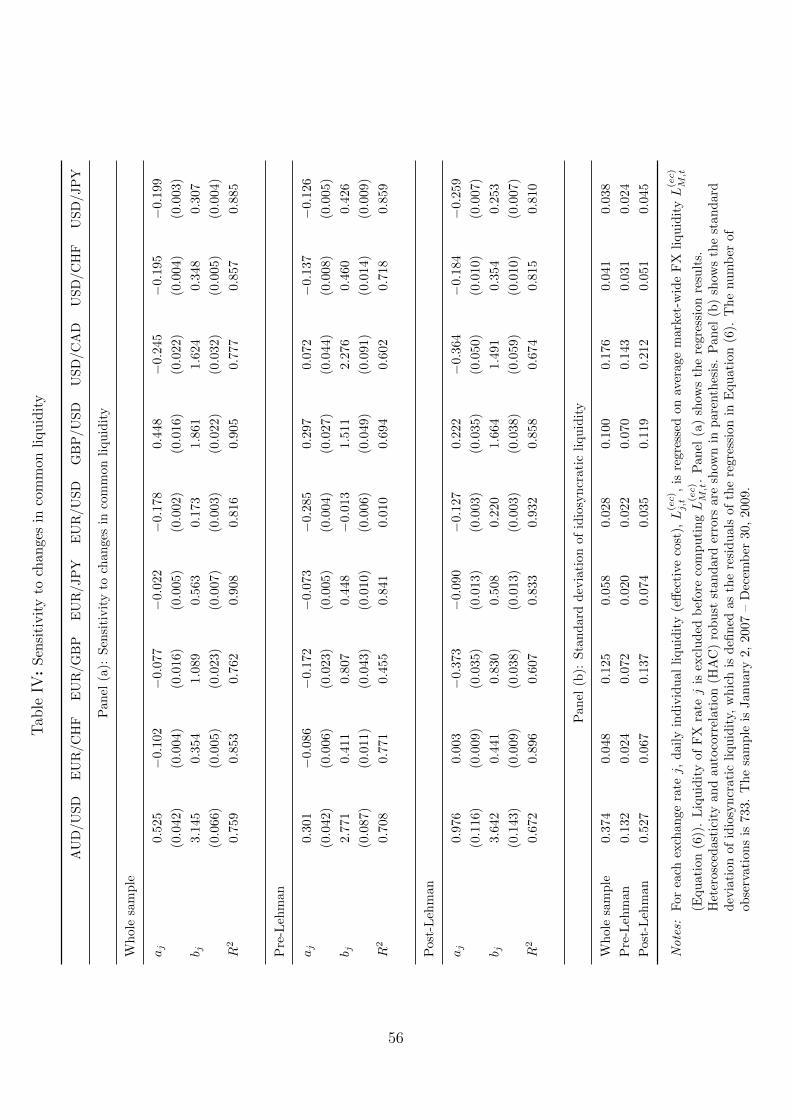
Tab
leIV
:S
ensi
tivit
yto
chan
ges
inco
mm
onli
qu
idit
y
AU
D/U
SD
EU
R/C
HF
EU
R/G
BP
EU
R/JP
YE
UR
/U
SD
GB
P/U
SD
US
D/C
AD
US
D/C
HF
US
D/JP
Y
Pan
el(a
):S
ensi
tivit
yto
chan
ges
inco
mm
on
liqu
idit
y
Wh
ole
sam
ple
aj
0.52
5−
0.10
2−
0.0
77
−0.0
22
−0.1
78
0.4
48
−0.2
45
−0.1
95
−0.1
99
(0.0
42)
(0.0
04)
(0.0
16)
(0.0
05)
(0.0
02)
(0.0
16)
(0.0
22)
(0.0
04)
(0.0
03)
b j3.
145
0.35
41.0
89
0.5
63
0.1
73
1.8
61
1.6
24
0.3
48
0.3
07
(0.0
66)
(0.0
05)
(0.0
23)
(0.0
07)
(0.0
03)
(0.0
22)
(0.0
32)
(0.0
05)
(0.0
04)
R2
0.75
90.
853
0.7
62
0.9
08
0.8
16
0.9
05
0.7
77
0.8
57
0.8
85
Pre
-Leh
man
aj
0.30
1−
0.08
6−
0.1
72
−0.0
73
−0.2
85
0.2
97
0.0
72
−0.1
37
−0.1
26
(0.0
42)
(0.0
06)
(0.0
23)
(0.0
05)
(0.0
04)
(0.0
27)
(0.0
44)
(0.0
08)
(0.0
05)
b j2.
771
0.41
10.8
07
0.4
48
−0.0
13
1.5
11
2.2
76
0.4
60
0.4
26
(0.0
87)
(0.0
11)
(0.0
43)
(0.0
10)
(0.0
06)
(0.0
49)
(0.0
91)
(0.0
14)
(0.0
09)
R2
0.70
80.
771
0.455
0.8
41
0.0
10
0.6
94
0.6
02
0.7
18
0.8
59
Pos
t-L
ehm
an
aj
0.97
60.
003
−0.3
73
−0.0
90
−0.1
27
0.2
22
−0.3
64
−0.1
84
−0.2
59
(0.1
16)
(0.0
09)
(0.0
35)
(0.0
13)
(0.0
03)
(0.0
35)
(0.0
50)
(0.0
10)
(0.0
07)
b j3.
642
0.44
10.
830
0.5
08
0.2
20
1.6
64
1.4
91
0.3
54
0.2
53
(0.1
43)
(0.0
09)
(0.0
38)
(0.0
13)
(0.0
03)
(0.0
38)
(0.0
59)
(0.0
10)
(0.0
07)
R2
0.67
20.
896
0.607
0.8
33
0.9
32
0.8
58
0.6
74
0.8
15
0.8
10
Pan
el(b
):S
tan
dard
dev
iati
on
of
idio
syncr
ati
cli
qu
idit
y
Wh
ole
sam
ple
0.37
40.
048
0.125
0.0
58
0.0
28
0.1
00
0.1
76
0.0
41
0.0
38
Pre
-Leh
man
0.13
20.
024
0.0
72
0.0
20
0.0
22
0.0
70
0.1
43
0.0
31
0.0
24
Pos
t-L
ehm
an0.
527
0.06
70.
137
0.0
74
0.0
35
0.1
19
0.2
12
0.0
51
0.0
45
Notes:
For
each
exch
ange
ratej,
dai
lyin
div
idu
al
liqu
idit
y(e
ffec
tive
cost
),L(ec)
j,t
,is
regre
ssed
on
aver
age
mark
et-w
ide
FX
liqu
idit
yL(ec)
M,t
(Equ
atio
n(6
)).
Liq
uid
ity
ofF
Xra
tej
isex
clu
ded
bef
ore
com
pu
tin
gL(ec)
M,t
.P
an
el(a
)sh
ows
the
regre
ssio
nre
sult
s.H
eter
osce
das
tici
tyan
dau
toco
rrel
atio
n(H
AC
)ro
bust
stan
dard
erro
rsare
show
nin
pare
nth
esis
.P
an
el(b
)sh
ows
the
stan
dard
dev
iati
onof
idio
syn
crat
icli
qu
idit
y,w
hic
his
defi
ned
as
the
resi
du
als
of
the
regre
ssio
nin
Equ
ati
on
(6).
Th
enu
mb
erof
obse
rvat
ion
sis
733.
Th
esa
mp
leis
Jan
uary
2,
2007
–D
ecem
ber
30,
2009.
56
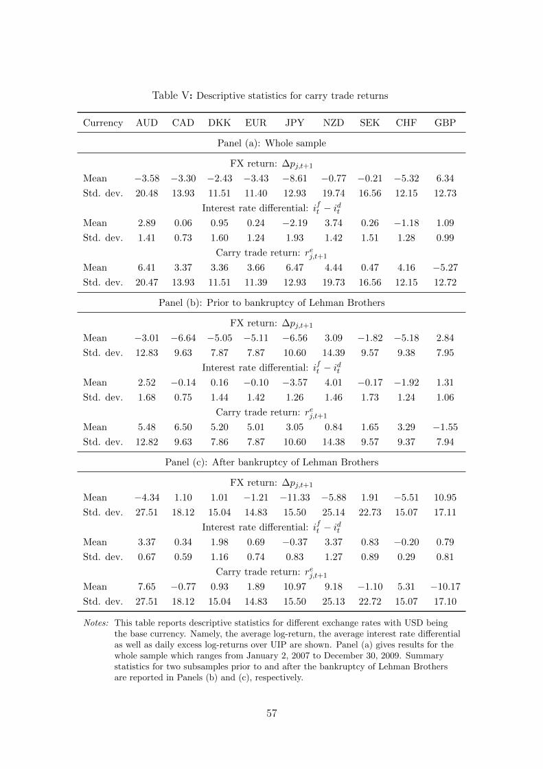
Table V: Descriptive statistics for carry trade returns
Currency AUD CAD DKK EUR JPY NZD SEK CHF GBP
Panel (a): Whole sample
FX return: ∆pj,t+1
Mean −3.58 −3.30 −2.43 −3.43 −8.61 −0.77 −0.21 −5.32 6.34
Std. dev. 20.48 13.93 11.51 11.40 12.93 19.74 16.56 12.15 12.73
Interest rate differential: ift − idtMean 2.89 0.06 0.95 0.24 −2.19 3.74 0.26 −1.18 1.09
Std. dev. 1.41 0.73 1.60 1.24 1.93 1.42 1.51 1.28 0.99
Carry trade return: rej,t+1
Mean 6.41 3.37 3.36 3.66 6.47 4.44 0.47 4.16 −5.27
Std. dev. 20.47 13.93 11.51 11.39 12.93 19.73 16.56 12.15 12.72
Panel (b): Prior to bankruptcy of Lehman Brothers
FX return: ∆pj,t+1
Mean −3.01 −6.64 −5.05 −5.11 −6.56 3.09 −1.82 −5.18 2.84
Std. dev. 12.83 9.63 7.87 7.87 10.60 14.39 9.57 9.38 7.95
Interest rate differential: ift − idtMean 2.52 −0.14 0.16 −0.10 −3.57 4.01 −0.17 −1.92 1.31
Std. dev. 1.68 0.75 1.44 1.42 1.26 1.46 1.73 1.24 1.06
Carry trade return: rej,t+1
Mean 5.48 6.50 5.20 5.01 3.05 0.84 1.65 3.29 −1.55
Std. dev. 12.82 9.63 7.86 7.87 10.60 14.38 9.57 9.37 7.94
Panel (c): After bankruptcy of Lehman Brothers
FX return: ∆pj,t+1
Mean −4.34 1.10 1.01 −1.21 −11.33 −5.88 1.91 −5.51 10.95
Std. dev. 27.51 18.12 15.04 14.83 15.50 25.14 22.73 15.07 17.11
Interest rate differential: ift − idtMean 3.37 0.34 1.98 0.69 −0.37 3.37 0.83 −0.20 0.79
Std. dev. 0.67 0.59 1.16 0.74 0.83 1.27 0.89 0.29 0.81
Carry trade return: rej,t+1
Mean 7.65 −0.77 0.93 1.89 10.97 9.18 −1.10 5.31 −10.17
Std. dev. 27.51 18.12 15.04 14.83 15.50 25.13 22.72 15.07 17.10
Notes: This table reports descriptive statistics for different exchange rates with USD beingthe base currency. Namely, the average log-return, the average interest rate differentialas well as daily excess log-returns over UIP are shown. Panel (a) gives results for thewhole sample which ranges from January 2, 2007 to December 30, 2009. Summarystatistics for two subsamples prior to and after the bankruptcy of Lehman Brothersare reported in Panels (b) and (c), respectively.
57
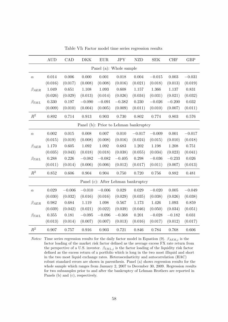
Table VI: Factor model time series regression results
AUD CAD DKK EUR JPY NZD SEK CHF GBP
Panel (a): Whole sample
α 0.014 0.006 0.000 0.001 0.018 0.004 −0.015 0.003 −0.031
(0.016) (0.017) (0.008) (0.008) (0.016) (0.021) (0.018) (0.013) (0.019)
βAER 1.049 0.651 1.108 1.093 0.608 1.157 1.366 1.137 0.831
(0.026) (0.029) (0.013) (0.014) (0.026) (0.034) (0.031) (0.021) (0.032)
βIML 0.330 0.197 −0.090 −0.091 −0.382 0.230 −0.026 −0.200 0.032
(0.009) (0.010) (0.004) (0.005) (0.009) (0.011) (0.010) (0.007) (0.011)
R2 0.892 0.714 0.913 0.903 0.730 0.802 0.774 0.803 0.576
Panel (b): Prior to Lehman bankruptcy
α 0.002 0.015 0.008 0.007 0.010 −0.017 −0.009 0.001 −0.017
(0.015) (0.019) (0.008) (0.008) (0.016) (0.024) (0.015) (0.010) (0.018)
βAER 1.170 0.605 1.092 1.092 0.683 1.202 1.198 1.208 0.751
(0.035) (0.043) (0.018) (0.018) (0.038) (0.055) (0.034) (0.023) (0.041)
βIML 0.288 0.226 −0.082 −0.082 −0.405 0.298 −0.036 −0.233 0.026
(0.011) (0.014) (0.006) (0.006) (0.012) (0.017) (0.011) (0.007) (0.013)
R2 0.852 0.606 0.904 0.904 0.750 0.720 0.756 0.882 0.481
Panel (c): After Lehman bankruptcy
α 0.029 −0.006 −0.010 −0.006 0.029 0.029 −0.020 0.005 −0.049
(0.030) (0.032) (0.016) (0.016) (0.029) (0.035) (0.038) (0.026) (0.038)
βAER 0.982 0.684 1.119 1.098 0.567 1.173 1.426 1.093 0.859
(0.039) (0.042) (0.021) (0.022) (0.039) (0.046) (0.050) (0.034) (0.051)
βIML 0.355 0.181 −0.095 −0.096 −0.368 0.201 −0.028 −0.182 0.031
(0.013) (0.014) (0.007) (0.007) (0.013) (0.016) (0.017) (0.012) (0.017)
R2 0.907 0.757 0.916 0.903 0.721 0.846 0.784 0.768 0.606
Notes: Time series regression results for the daily factor model in Equation (9). βAER,j is thefactor loading of the market risk factor defined as the average excess FX rate return fromthe perspective of a U.S. investor. βIML,j is the factor loading of the liquidity risk factordefined as the excess return of a portfolio which is long in the two most illiquid and shortin the two most liquid exchange rates. Heteroscedasticity and autocorrelation (HAC)robust standard errors are shown in parenthesis. Panel (a) shows regression results for thewhole sample which ranges from January 2, 2007 to December 30, 2009. Regression resultsfor two subsamples prior to and after the bankruptcy of Lehman Brothers are reported inPanels (b) and (c), respectively.
58