Louisiana State UniversityLSU Digital Commons

LSU Doctoral Dissertations Graduate School

2007

Liquidity and speculative trading: evidence fromstock price adjustments to quarterly earningsannouncementsHsiao-Fen YangLouisiana State University and Agricultural and Mechanical College

Follow this and additional works at: https://digitalcommons.lsu.edu/gradschool_dissertations

Part of the Finance and Financial Management Commons

This Dissertation is brought to you for free and open access by the Graduate School at LSU Digital Commons. It has been accepted for inclusion inLSU Doctoral Dissertations by an authorized graduate school editor of LSU Digital Commons. For more information, please contactgradetd@lsu.edu.

Recommended CitationYang, Hsiao-Fen, "Liquidity and speculative trading: evidence from stock price adjustments to quarterly earnings announcements"(2007). LSU Doctoral Dissertations. 3742.https://digitalcommons.lsu.edu/gradschool_dissertations/3742

LIQUIDITY AND SPECULATIVE TRADING: EVIDENCE FROMSTOCK PRICE ADJUSTMENTS TO QUARTERLY EARNINGS

ANNOUNCEMENTS

A Dissertation

Submitted to the Graduate Faculty of theLouisiana State University and

Agricultural and Mechanical Collegein partial fulfillment of the

requirements for the degree ofDoctor of Philosophy

in

The Interdepartmental Program in Business Administration

byHsiao-Fen Yang

B.B.A., National Taiwan University, 1998M.B.A., National Central University, 2000

August 2007

Acknowledgments

I would like to thank my committee chair, Dr. Ji-Chai Lin , for his great guidance

and help. I also would like to express my heartfelt gratitude to Dr. Gary Sanger for his

invaluable comments and suggestions. I am deeply indebted to other committee members

of my dissertation: Dr. Wei Li, Dr. Robert Newman, and Dr. Angela Woodland for

their helpful comments. Special thanks also go to other faculty members and staffs in the

Department of Finance, especially Dr. William Lane and Dr. Jimmy Hilliard, for their help

and support. Without the guidance and assistance from these individuals, this dissertation

would not have been completed.

In this lengthy studying process, I have also benefited from the support of my family

members and colleagues. I truly appreciate the support of my mother, my father, my

brother, and my sister. I am especially grateful to my mother for her encouragement

whenever I am stressed out. I also thank my colleagues in the finance department, especially

Huihua Li, Tung-Hsiao Yang, and Fan Chen, for their support and friendship.

ii

Table of Contents

Acknowledgments. . . . . . . . . . . . . . . . . . . . . . . . . . . . . . ii

List of Tables . . . . . . . . . . . . . . . . . . . . . . . . . . . . . . . v

List of Figures . . . . . . . . . . . . . . . . . . . . . . . . . . . . . . . vii

Abstract . . . . . . . . . . . . . . . . . . . . . . . . . . . . . . . . . ix

Chapter 1. Introduction . . . . . . . . . . . . . . . . . . . . . . . . . . . 1

Chapter 2. Literature Review . . . . . . . . . . . . . . . . . . . . . . . . 82.1 Liquidity, Risk, and Stock Return . . . . . . . . . . . . . . . . . . . 8

2.1.1 Dimensions of Liquidity . . . . . . . . . . . . . . . . . . . . . 82.1.2 Liquidity Risk . . . . . . . . . . . . . . . . . . . . . . . . . 11

2.2 Liquidity, Irrational Behavior, and Stock Returns . . . . . . . . . . . . 122.2.1 Evidence of Sentiment and Overconfidence . . . . . . . . . . . . . 132.2.2 Liquidity, Sentiment/Overconfidence, and Stock Returns . . . . . . . 17

2.3 Liquidity and Quarterly Earnings Announcement . . . . . . . . . . . . 20

Chapter 3. Empirical Prediction . . . . . . . . . . . . . . . . . . . . . . . 24

Chapter 4. Data and Research Design . . . . . . . . . . . . . . . . . . . . . 314.1 Data . . . . . . . . . . . . . . . . . . . . . . . . . . . . . . . 314.2 Research Design . . . . . . . . . . . . . . . . . . . . . . . . . . 344.3 Descriptive Statistics . . . . . . . . . . . . . . . . . . . . . . . . 37

Chapter 5. Empirical Results . . . . . . . . . . . . . . . . . . . . . . . . 415.1 Abnormal Return around Earnings Announcement. . . . . . . . . . . . 415.2 Robustness Check for Abnormal Return . . . . . . . . . . . . . . . . 44

5.2.1 Control for Size and Book-to-Market . . . . . . . . . . . . . . . 455.2.2 Control for Misperceptions of Future Earnings . . . . . . . . . . . 495.2.3 Control for Information Available, Dispersion in Opinions, and Infor-

mativeness of Announcements . . . . . . . . . . . . . . . . . . 585.2.4 Control for Changes of Future Liquidity . . . . . . . . . . . . . . 685.2.5 Control for Changes in Risk . . . . . . . . . . . . . . . . . . . 695.2.6 Use Market-Adjusted Return, Use Only NYSE/AMEX Stocks, and

Use Only Announcements with Trade on Day -2 . . . . . . . . . . 725.2.7 Subperiod Analysis . . . . . . . . . . . . . . . . . . . . . . . 83

iii

5.2.8 Summary of Robustness Checks . . . . . . . . . . . . . . . . . 845.3 Abnormal Volume around Earnings Announcements . . . . . . . . . . . 895.4 Robustness Check for Abnormal Volume . . . . . . . . . . . . . . . . 925.5 Liquidity Premium Realized during Quarterly Earnings Announcement Pe-

riods . . . . . . . . . . . . . . . . . . . . . . . . . . . . . .1015.6 Multivariate Regression . . . . . . . . . . . . . . . . . . . . . . .107

Chapter 6. Conclusion . . . . . . . . . . . . . . . . . . . . . . . . . . .124

References . . . . . . . . . . . . . . . . . . . . . . . . . . . . . . . . .127

Vita . . . . . . . . . . . . . . . . . . . . . . . . . . . . . . . . . . .131

iv

List of Tables

1 Summary Statistics . . . . . . . . . . . . . . . . . . . . . . . . . 38

2 Quarterly Earnings Announcement Effect on Stock Return . . . . . . . . 42

3 Robustness Check for Earnings Announcement Effect on Stock Return: Con-trol for Size and Book-to-Market . . . . . . . . . . . . . . . . . . . . 46

4 Robustness Check for Earnings Announcement Effect on Stock Return: Con-trol for Misperceptions of Future Earnings . . . . . . . . . . . . . . . . 53

5 Robustness Check for Earnings Announcement Effect on Stock Return: Con-trol for Information Available, Dispersion in Opinions, and Informativenessof Announcements . . . . . . . . . . . . . . . . . . . . . . . . . . 60

6 Robustness Check for Earnings Announcement Effect on Stock Return: Con-trol for Change of Liquidity . . . . . . . . . . . . . . . . . . . . . . 70

7 Robustness Check for Earnings Announcement Effect on Stock Return: Con-trol for Change of Risk . . . . . . . . . . . . . . . . . . . . . . . . 73

8 Robustness Check for Earnings Announcement Effect on Stock Return: UseMarket-Adjusted Return, Include Only NYSE/AMEX Stocks, and IncludeOnly Announcements with Trade on Day −2. . . . . . . . . . . . . . . 78

9 Robustness Check for Earnings Announcement Effect on Stock Return: Sub-period Analysis . . . . . . . . . . . . . . . . . . . . . . . . . . . 85

10 Quarterly Earnings Announcement Effect on Trading Volume . . . . . . . 90

11 Robustness Check for Earnings Announcement Effect on Stock Volume . . . 94

12 Liquidity Premium Realized during Quarterly Earnings Announcement Pe-riods . . . . . . . . . . . . . . . . . . . . . . . . . . . . . .102

13 Liquidity Premium Realized during Quarterly Earnings Announcement Pe-riods in Different Quarters . . . . . . . . . . . . . . . . . . . . . .105

v

14 Summary Statistics of Regression Variables . . . . . . . . . . . . . . .110

15 Multivariate Regression . . . . . . . . . . . . . . . . . . . . . . .114

16 Robustness Check of Multivariate Regression . . . . . . . . . . . . . .119

vi

List of Figures

1 Cumulative Abnormal Return during Quarterly Earnings Announcement Pe-riod . . . . . . . . . . . . . . . . . . . . . . . . . . . . . . 43

2 Cumulative Abnormal Return during Quarterly Earnings Announcement Pe-riod: Control for Size . . . . . . . . . . . . . . . . . . . . . . . . . 47

3 Cumulative Abnormal Return during Quarterly Earnings Announcement Pe-riod: Control for Book-to-Market. . . . . . . . . . . . . . . . . . . . 50

4 Cumulative Abnormal Return during Quarterly Earnings Announcement Pe-riod: Control for Forecast Error . . . . . . . . . . . . . . . . . . . . 54

5 Cumulative Abnormal Return during Quarterly Earnings Announcement Pe-riod: Control for Growth Revision . . . . . . . . . . . . . . . . . . . 56

6 Cumulative Abnormal Return during Quarterly Earnings Announcement Pe-riod: Control for Analysts Following . . . . . . . . . . . . . . . . . . 62

7 Cumulative Abnormal Return during Quarterly Earnings Announcement Pe-riod: Control for Forecast Dispersion . . . . . . . . . . . . . . . . . . 64

8 Cumulative Abnormal Return during Quarterly Earnings Announcement Pe-riod: Control for Change in Volatility . . . . . . . . . . . . . . . . . . 67

9 Cumulative Abnormal Return during Quarterly Earnings Announcement Pe-riod: Control for Changes of Liquidity . . . . . . . . . . . . . . . . . 71

10 Cumulative Abnormal Return during Quarterly Earnings Announcement Pe-riod: Control for Changes of βMKTRF . . . . . . . . . . . . . . . . . . 74

11 Cumulative Abnormal Return during Quarterly Earnings Announcement Pe-riod: Control for Changes of βSMB . . . . . . . . . . . . . . . . . . . 75

12 Cumulative Abnormal Return during Quarterly Earnings Announcement Pe-riod: Control for Changes of βHML . . . . . . . . . . . . . . . . . . . 76

vii

13 Cumulative Abnormal Return during Quarterly Earnings Announcement Pe-riod: Use Market-Adjusted Return as Abnormal Return . . . . . . . . . . 80

14 Cumulative Abnormal Return during Quarterly Earnings Announcement Pe-riod for NYSE/AMEX Stocks . . . . . . . . . . . . . . . . . . . . . 81

15 Cumulative Abnormal Return during Quarterly Earnings Announcement Pe-riod: Use Only Announcements with Trade on Day −2 . . . . . . . . . . 82

16 Cumulative Abnormal Return around Quarterly Earnings Announcementduring Internet Bubble Period . . . . . . . . . . . . . . . . . . . . . 86

17 Cumulative Abnormal Return around Quarterly Earnings Announcementduring Non-Bubble Period . . . . . . . . . . . . . . . . . . . . . . 87

18 Cumulative Abnormal Volume during Quarterly Earnings AnnouncementPeriod . . . . . . . . . . . . . . . . . . . . . . . . . . . . . . . 91

19 Cumulative Abnormal Volume during Quarterly Earnings Announcement Pe-riod: One-Factor Market Model . . . . . . . . . . . . . . . . . . . . 96

20 Cumulative Abnormal Volume during Quarterly Earnings Announcement Pe-riod for NYSE/AMEX Stocks . . . . . . . . . . . . . . . . . . . . . 97

21 Cumulative Abnormal Volume around Quarterly Earnings Announcementduring Internet Bubble Period . . . . . . . . . . . . . . . . . . . . . 99

22 Cumulative Abnormal Volume around Quarterly Earnings Announcementduring Non-Bubble Period . . . . . . . . . . . . . . . . . . . . . .100

viii

Abstract

This dissertation studies whether stock price reactions to quarterly earnings announce-

ments depend on stock liquidity. Baker and Stein (2004) and Scheinkman and Xiong (2003)

develop models showing that liquidity can be affected by investor sentiment or speculative

trading. With short-sale constraints, liquid stocks have more trading from optimistic,

overconfident investors and tend to be overvalued. In this study, we hypothesize that if a

liquid stock is overpriced due to intensive speculative trading, the overpricing should be

corrected partially or fully after quarterly earnings announcements which convey the in-

formation about the fundamental value of stocks and synchronize investors’ adjustment to

mispricing. Our results show that liquid stocks earn significant lower abnormal returns at

the announcements than illiquid stocks. Furthermore, prior to the announcements, liquid

stocks also have significant speculative trading. After controlling for other determinants of

abnormal returns, we find the return difference between liquid and illiquid stocks during

the 12-day earnings announcement period is 4.11%, which is about one-third of the annual

liquidity premium. Our findings suggest that the effect of investors’ speculative behavior

on stock prices is not negligible and that earnings announcements serve as an important

mechanism for regulating overpricing caused by speculative trading.

ix

Chapter 1 Introduction

The effect of liquidity on stock returns has been a subject of research for over two

decades. In a rational asset pricing framework, investors require a higher return for illiquid

stocks than for liquid stocks in order to compensate the extra liquidity risk and transaction

costs. Amihud and Mendelson (1986) develop a model which shows that the expected return

of an asset increases with the transaction costs and find supportive empirical evidence.

Recent studies such as Pastor and Stambaugh (2003), Acharya and Pedersen (2005), and

Liu (2006) all suggest that liquidity risk plays an important role in asset pricing. These

studies indicate that the liquidity premium is driven by the high required rate of return and

low valuation of illiquid stocks. On the contrary, Baker and Stein (2004) and Scheinkman

and Xiong (2003) who assume investors are overconfident develop models which show that

liquidity can be an indicator of investor sentiment or speculative trading. Liquid stocks

have more trading from optimistic overconfident investors and tend to be overvalued. Baker

and Stein (2004) and Scheinkman and Xiong (2003) imply that the liquidity premium can

also be partially driven by overpriced liquid stocks.

Motivated by Baker and Stein (2004) and Scheinkman and Xiong (2003), this dis-

sertation investigates whether stock price reactions to quarterly earnings announcements

depend on stock liquidity. The investigation allows us to assess the importance of specu-

lative trading on liquidity and the role of quarterly earnings announcements in regulating

speculative trading. We focus on the revision of the mispricing after quarterly earnings

announcements because quarterly earnings announcements provide information about firm

1

valuation and give investors a chance to correct mispricing. When overconfident investors

find the signal they get before the announcement is far from the value revealed in the fi-

nancial report, they learn that their own information is not as informative as they thought

it should be. Therefore, after the announcements, they may perceive their mispricing and

correct it. Besides, investors who know the stock is overpriced (underpriced) prior to the

announcement may not sell (buy) the stock immediately if they think the magnitude of

mispricing will continue increasing for a while. However, expecting the mispricing may be

revised after quarterly announcements, they may want to sell (buy) stocks synchronically

during the announcement period1. Therefore, quarterly earnings announcements can serve

as a mechanism for regulating mispricing caused by speculative trading.

In this study, we hypothesize that if liquid stocks are overpriced, right after quarterly

earnings announcements they should have lower abnormal returns than illiquid stocks.

Our hypothesis depend on two assumptions. First, we posit that investors adjust their

mispricing after quarterly earnings announcements. Second, we assume that liquid stocks

tend to have more speculative trading by optimistic overconfident investors and are more

likely to be overvalued. This assumption is derived from Baker and Stein (2004) and

Scheinkman and Xiong (2003). Baker and Stein (2004) develop a model which links liquidity

with subsequent stock returns. They show that with short-sale constraints, an increase in

liquidity indicates that the market is dominated by overconfident investors whose valuation

1Abreu and Brunnermeier (2003) argue that when rational arbitrageurs perceive a bubble, they knowthe market will eventually collapse. However, if the bubble will not burst soon, they would like to ride thebubble and then sell the bubble asset right before the bubble crashes. To burst the bubble, there must bea sufficient number of arbitrageurs selling the bubble asset at the same time. Because arbitrageurs havedifferent opinions about the timing of the bubble, it is difficult for them to synchronize their sales. As aresult, the bubble persists until a synchronizing event which induces a sufficient number of arbitrageurs tosell their assets.

2

of a stock is higher than its fundamental value. From Baker and Stein (2004), we can infer

a positive relation between active trading activities and the overpricing of a stock.

Scheinkman and Xiong (2003) provide a model which directly shows a positive relation

between cross-sectional trading activities and a speculative component of stock prices. In

their model, investors are overconfident and have different beliefs. When there are short-

sale constraints, the ownership of a share of stock gives investors an American-type re-

sale option. Expecting to sell their shares in the future to other investors who have more

optimistic beliefs (a greater fool), investors are willing to pay a price that is higher than their

subjective valuation of the firm’s fundamental value. As a result, a speculative component,

the difference between the transaction price and the asset’s fundamental value, is embedded

in the stock price. Scheinkman and Xiong (2003) show that in cross section, when the degree

of overconfidence is higher, investors trade more frequently and the speculative component

is larger. This indicates that liquidity of stocks is magnified by speculative trading of

overconfident investors and that liquid stocks tend to be more overvalued than illiquid

stocks.

If liquidity and stock prices are affected by speculative trading and investors ad-

just their mispricing around quarterly earnings announcements, we should observe a lower

return for liquid stocks than for illiquid stocks during the announcement periods. Further-

more, because quarterly earnings announcements are scheduled announcements, investors

anticipate the upcoming events before the announcements. During the period right before

the announcements, information asymmetry increases. Trading volume decreases because

discretionary liquidity traders are unwilling to trade with informed investors and will

3

postpone their transactions until news release. If the increase in information asymmetry

enlarges the differences in beliefs among overconfident investors, in Scheinkman and Xiong’s

(2003) framework, we should observe more speculative trading during this period. Because

liquid stocks tend to have more speculative trading, in this study we also test whether the

decrease, if any, in volume for liquid stocks prior to quarterly earnings announcements is

lower than the volume decrease for illiquid stocks.

Investigating the announcement effects of about 260,000 quarterly announcements

made during 1982-2004 by firms listed in NYSE, AMEX, and NASDAQ, we find evidence

supports our hypotheses. The abnormal returns right after quarterly earnings announce-

ments decrease with the liquidity of the stock. The differences of the cumulative abnormal

returns between the most liquid stocks and the least liquid stocks is 1.91% and is signif-

icant during the 3-day period from day 0 to day 2. This result is robust after we control

for book-to-market, analysts’ forecast errors, revisions of growth forecasts, analyst forecast

dispersions, changes of return volatility, changes of future liquidity, and for changes in risk.

Our results also hold well for small and median stocks and for firms with low or median ana-

lysts following. For large stocks, however, the differences of the 3-day cumulative abnormal

returns between liquid and illiquid stocks are not significant. Because larger firms tend to

have less subjective valuation, they are less likely to be affected by investor sentiment than

small firms. Therefore, our result is not surprising because large firms are not attractive

to speculators. For firms with high analysts following, we also do not find a significant re-

sult. Because high-following firms usually have frequent news releases from analysts, which

boosts the trading activities, the sample size for high-following illiquid firms is very small.

4

These firms may suffer from firm-specific problems such as financial distress which deter

investors from trading.

Examining the abnormal volume before earnings announcements, we find the trading

volume decreases prior to the quarterly earnings announcements. The drop in volume de-

creases with the liquidity of the stocks. From the path of cumulative abnormal returns and

the changes of trading volume during the period from day -10 to day 10, we find evidences

of speculative trading for the liquid stocks. Their cumulative abnormal returns increase

significantly prior to the announcements but decrease significantly after announcements.

Because we do not observe the same pattern for illiquid stocks and the decrease in trading

volume prior to the announcements for liquid stocks is lower than illiquid stocks, the re-

sult indicates that before the announcements, speculative trading occurs more frequently

for liquid stocks. This pattern of speculative trading holds particularly for small, growth,

high-forecast-dispersion, low-analyst-following stocks, which supports Baker and Wurgler

(2006).

In the further analysis of the different announcement effects on liquid and illiquid

stocks, we find liquidity premium realized during the 12-day announcement period is 5.54%.

It is about 45.6% of the annual liquidity premium. The liquidity risk or transaction cost

story alone seems not enough to explain why 45.6% of annual liquidity premium is realized

during only 12 days of the year. Because the liquidity premium realized around quarterly

earnings announcements may also reflect differences of information content between the

announcements of liquid firms and announcements of illiquid firms, we construct a regres-

sion of cumulative abnormal returns on the measure of liquidity as well as information

5

content of the announcements and other firm characteristics. We find the coefficient of the

liquidity measure is significant. After controlling for possible factors of abnormal returns

around quarterly earnings announcements, we still find about 4.11 % premium per year

(about one-third annual liquidity premium) occurs during the 12-day announcement pe-

riod. Again the magnitude is not trivial. These results indicate that liquidity premium can

be partially driven by the speculative trading from overconfident investors.

This study is related to several empirical studies which show the relation between

trading activities and stock returns. Johnson, Lei, Lin, and Sanger (2006) show the effect

of the time-series changes of volume on stock returns. The focus of this study is different

from that of Johnson, Lei, Lin, and Sanger (2006) in that we study the different response

to quarterly earnings announcements between liquid and illiquid stocks and show the re-

lation between cross-sectional differences of trading activities and stock returns. Lee and

Swaminathan (2000) also provide the abnormal returns for high-volume and low-volume

stocks around earnings announcements and argue that higher future returns experienced

by low volume stocks are related to investor misperceptions about future earnings. Here

we investigate whether speculative trading, in addition to investors’ misperceptions about

future earnings, affects announcement returns and trading volume around earnings an-

nouncements. We control the misperceptions documented by Lee and Swaminathan (2000)

and test whether stocks with high trading activities have speculative trading and low an-

nouncement returns. Piqueira (2006) tests whether liquid stocks are overvalued based on

monthly cross-sectional regressions of returns on lagged trading activities as well as other

control variables. In this study, we focus on the revision of mispricing and speculative

6

trading around quarterly earnings announcements. Frazzini and Lamont (2006) link trad-

ing volume during past earnings announcement periods with the returns of the subsequent

announcements; while we use the cross-sectional liquidity at the end of June each year as

a measure of speculative trading and test the relation between speculative trading and the

announcement returns during the following year.

Our findings contribute to the debate on whether investors’ behavior affects stock

prices. First, we document significant speculative trading on liquid stocks but not on

illiquid stocks. Second, we find a non-trivial magnitude of the perceived liquidity pre-

mium resulted from non-fundamental non-risk factors realized during quarterly earnings

announcements. This indicates that earnings announcements do serve as an important

mechanism for revising overpricing caused by speculative trading. The evidence that spec-

ulative trading by overconfident investors affects stock prices suggests that incorporating

investors’ speculative behavior into an asset pricing model is a promising area for future

research.

The rest of this dissertation proceeds as follows. Chapter 2 reviews literatures related

to this study. Chapter 3 presents the empirical predictions. In chapter 4, we briefly describe

the sources of data, research design, and sample characteristics. The empirical results are

shown in chapter 5. Chapter 6 concludes.

7

Chapter 2 Literature Review

This dissertation investigates whether stock price reactions to quarterly earnings an-

nouncements depend on stock liquidity. The investigation allows us to assess the impor-

tance of speculative trading on liquidity and the role of quarterly earnings announcements

in regulating speculative trading. We argue that quarterly earnings announcements provide

information about firms’ fundamental value to the public and thus give investors a chance

to review the precision of their own information. Furthermore, the announcements pro-

vide possible timing for investors who know the overpricing (underpricing) to synchronize

their revisions and generate a sufficient selling (buying) force to correct the mispricing.

Therefore, if liquid stocks are overpriced due to intensive speculative trading, its abnormal

return should be lower than illiquid stocks right after the quarterly announcements. In

this chapter, we review related literature. We first review the role of liquidity under the

rational asset pricing framework. Then we go on to the framework with the existence of

irrational investors. We focus on the effects of irrational behavior on liquidity and stock

returns. In the last section, we review papers related to the changes of liquidity during

quarterly earnings announcements, the particular period we are interested in.

2.1 Liquidity, Risk, and Stock Return

2.1.1 Dimensions of Liquidity

Liquidity is usually referred to the ability to buy or sell an asset quickly at low cost

without much change in value. The standard asset pricing model usually assumes that

market is perfect. Under this assumption, liquidity does not affect asset prices. However,

8

because the market is not frictionless, illiquid stocks are usually associated with high trans-

action costs, less information available, and great difficulty in executing orders. As a result,

investors usually require a higher return for illiquid stocks.

From the definition of liquidity, there are four dimensions of liquidity: trading cost,

price impact, trading volume, and trading speed.

Trading cost: When the trading cost of a stock is higher, the liquidity of that stock is

lower. Amihud and Mendelson (1986) develop a model which shows the effect of the bid-ask

spread on asset pricing. In their model, investors who buy an asset expect to sell it and pay

transaction costs in the future. Therefore, the stock price is the expected present value of

all future dividends minus the expected present value of all future transaction costs. Their

model predicts that the expected return of an asset increases with the transaction cost.

Using data over the period 1961-1980 for NYSE stocks, they find high-spread stocks earn

higher returns than low-spread stocks after controlling for firm size and market risk, which

is consistent with the prediction of their model.

Price impact: Price impact is the change of price caused by a trade. When a stock shows

a higher price impact, it is more illiquid. Using ISSM data in 1984 and 1988, Brennan and

Subrahmanyam (1996) estimate Kyle’s (1985) price-impact parameter, λ, by regressing the

trade by trade price change on the signed transaction size. Then they sort NYSE stocks and

form portfolios based on λ and examine the relation between λ and stock return during

1984-1991. Their results show that high-λ stocks earn significantly higher returns than

low-λ stocks. Considering that the intraday data does not cover a long period of time,

Amihud (2002) proposes a new price impact measure (measure of illiquidity) which can

9

be estimated from daily data. He defines the measure as the daily ratio of absolute stock

return to its dollar volume, averaged over some period of time. Examining returns of the

NYSE stocks during 1964-1997, he also finds stocks with a higher price impact measure

earn higher returns.

Trading volume: When a stock is traded more frequently, it is easier for traders to

close their position and thus it is more liquid. According to the liquidity hypothesis,

firms with relatively low trading volume should offer a higher expected return. Datar,

Naik, and Radcliffe (1998) examine the relation between turnover of NYSE stocks and

their returns during 1963-1991. They show that low turnover stocks earn higher returns

than high turnover stocks after controlling for size, book-to-market ratio, and beta. When

investors reduce their trading frequency, the average holding period of the stocks, which

is the reciprocal of the stock turnover, is prolonged. They argue that this result supports

Amihud and Mendelson’s (1986) prediction that less liquid stocks are allocated to investors

with longer holding periods and should earn a higher return. Using a regression model which

examines the relation between risk-adjusted returns to common risk factors and several firm

specific characteristics, Brennan, Chordia, and Subrahmanyam (1998) also find a negative

relation between trading activities and stock returns for both NYSE/AMEX and NASDAQ

stocks during 1966-1995.

Trading speed: When the order of a stock can be executed faster, that stock is more

liquid. Liu (2006) proposes a new liquidity measure, LM12, to capture trading quantity,

trading cost, and trading speed at the same time, with a particular focus on the trading

speed. He defines LM12 as the standardized turnover-adjusted number of zero daily trading

10

volume over the prior 12 months. High-LM12 stocks do not have trades every day and are

illiquid. His results show that for NYSE/AMEX stocks, stocks in the highest LM12 decile

significantly outperform stocks in the lowest LM12 decile by 0.682% per month over a

12-month holding period. After controlling for size, book-to-market, turnover, and past

returns, this liquidity premium is still robust.

2.1.2 Liquidity Risk

In addition to studies which focus on the relation between stock returns and different

dimensions of liquidity, many papers investigate whether liquidity is a common risk factor.

Pastor and Stambaugh (2003) argue that when the market-wide liquidity is low, investors

who face a solvency constraint require higher expected returns for holding illiquid assets.

They introduce the aggregate liquidity of the market to the asset pricing model and find

stocks with high sensitivities to changes of market liquidity earn higher returns than stocks

with low sensitivities by 7.5 percent per year during 1966-1999 after the adjustment for

exposures to the market return, size, value, and momentum factors. Their finding shows

that market-wide liquidity is an important state variable for asset pricing.

Acharya and Pedersen (2005) propose liquidity-adjusted CAPM which introduces

three liquidity betas. The first liquidity beta captures the commonality in liquidity with

the market liquidity and is positive for most securities . This indicates that expected return

increases with the covariance between the asset’s illiquidity and the market illiquidity. The

second liquidity beta measures the co-movement of the return of asset i with the market-

wide illiquidity. It is usually negative because a rise in market illiquidity reduces asset

values. The third liquidity beta shows the liquidity sensitivity to market returns. It is

11

usually negative for most stocks because investors are willing to accept a lower expected

return on a security that is liquid in a down market. Using Amihud’s (2002) illiquidity

measure to proxy for the illiquidity for NYSE/AMEX stocks during 1963-1999, Acharya

and Pedersen (2005) find evidence supports their model.

Unlike prior studies which use liquidity measures as pricing factors, Liu (2006) con-

structs a liquidity factor from mimicking portfolios of his liquidity measure, LM12. He

documents that the mimicking liquidity factor is highly negative correlated with the mar-

ket and should be a state variable in asset pricing. In his paper, he proposes a two-factor

augmented CAPM that includes both market and liquidity factors. Compared with CAPM

and Fama and French 3-factor model, his two-factor model is more powerful because it cap-

tures the liquidity risk and explains well for various anomalies such as size premium, value

premium, effects of earnings-to-price on stock returns, and returns on long-term contrarian

strategies. His results suggest that liquidity risk is an important factor in asset pricing.

Although the liquidity risk can explain the liquidity premium found in prior studies,

there is another stream of papers studying the possibility that the liquidity is affected by

irrational investors. As a result, the low return of liquid stocks can be partially driven by

irrational investors’ revision of their mispricing. This indicates that the liquidity premium

may not solely result from the liquidity risk. In next section, we review the relation between

liquidity and irrational investors’ behavior proposed by literature.

2.2 Liquidity, Irrational Behavior, and Stock Returns

Under a frictionless world, irrational investors’ behavior does not affect asset prices

because arbitrageurs trade immediately and then force the stock price to converge to its

12

fundamental value. However, in the real world, arbitrage is limited. Miller (1977) points

out that in the presence of a short-sale constraint, the stock price is overpriced because

pessimistic investors cannot sell the stock. Black (1986) argues that informed traders do

not take large enough positions to eliminate the mispricing because their information does

not guarantee profits. Taking a large position is too risky. Campbell and Kyle (1993) posit

that noise traders affect prices because fundamental risk deters smart-money investors

from aggressively betting against noise traders. Shleifer and Vishny (1997) suggest that

arbitrageurs can only specialize a small group of stocks and they avoid to take extremely

volatile arbitrage position because their capital providers use their performance to ascertain

their ability to invest profitably. Due to the above limits of arbitrage, stock prices are

affected by irrational investors.

In the following subsections, we review how irrational behavior affects liquidity and

returns. We first review evidences of investor sentiment and overconfidence from prior

studies. Then we review relations among liquidity, sentiment/overconfidence, and stock

returns both in time series and in cross section.

2.2.1 Evidence of Sentiment and Overconfidence

In this subsection, we focus on two sources of heterogeneous beliefs between rational

and irrational investors: sentiment and overconfidence. Sentiment could lead to the dif-

ferences in valuation between rational investors and irrational investors. When investor

sentiment is high and investor valuations of stocks are dispersed, stock prices could be

overvalued if there is a short-sale constraint. Using different measures of sentiment, many

studies have found evidences that sentiment affects stock prices:

13

Closed-end fund discounts, ratio of odd-lot sales to purchases, and net mu-

tual fund redemption: Individual investors are more likely to be affected by sentiment.

Because the investors of mutual fund and traders of odd lots are usually individual in-

vestors, closed-end fund discounts, ratio of odd-lot sales to purchases, and net mutual fund

redemption can be used as measures of general investor sentiment. Neal and Wheatley

(1998) examine whether these three measures can predict returns. They find little relation

between the odd-lot ratio and stock returns. However, they find closed-end fund discounts

and net redemption can predict size premium. Specifically, they find closed-end fund dis-

counts and net fund redemption are both positive related to returns on small firms. On the

contrary, on large firms, the relation between closed-end fund discounts and returns is not

significant and the relation between net redemption and returns is negative. These results

indicate that when closed-end fund discounts and net redemption are higher, size premium

is higher, which supports the hypothesis that investor sentiment affects stock returns.

Buy-sell imbalance of retail investors: Because individual investors are subject to

investor sentiment, their trading activities reflect their sentiment. Using the transaction

data of retail investors at a major U.S. discount brokerage house over the period 1991 to

1996, Kumar and Lee (2006) construct a buy-sell imbalance (BSI) measure for different

stock portfolios to proxy changes in retail sentiment. They find BSI can predict stock

returns. For small stocks, low-price stocks, firms with low institutional ownership, and

value stocks, the retail concentrations and retail trading activities are extraordinarily high.

These stocks also have significantly positive factor loadings on BSI. Besides, they also find

individual investors tend to buy or sell stocks in concert. When one set of retail investors

14

buy (sells) stocks, another set of retail investors also tends to buy (sell) stocks. Their

evidence shows that retail investors are affected by sentiment and their sentiment affects

stock returns.

Bull-bear spread: Using “bull-bear spread” from a direct survey data to measure investor

sentiment, Brown and Cliff (2005) investigate the effect of sentiment on stock returns. They

find sentiment appears to have little predictive power for subsequent near-term returns.

However, sentiment does have effect on long-term stock returns. High levels of sentiment

lead to significantly lower returns over the next two or three years. A one standard deviation

of bullish shock to sentiment results in a subsequent underperformance of the market by

7% over the next three years. This indicates that asset values are affected by investor

sentiment and market prices revert to fundamental values over several years.

Sentiment Index: Baker and Wurgler (2005) propose a sentiment index to measure

investor sentiment at the market level. The sentiment index is constructed based on the

first principal component of six sentiment proxies: closed-end fund discounts, NYSE share

turnover, the number of IPOs, the average first-day returns of IPOs, the share of equity

issues in total equity and debt issues, and the dividend premium. They predict that a

broad sentiment wave on the market can have different effects on stocks because sentiment-

based demand shocks and arbitrage constraints differ across stocks. Stocks that are likely

to be most sensitive to speculative demand also tend to be the riskiest and costliest to

arbitrage. Therefore, prices of those stocks tend to be overvalued when investor sentiment

is high and their subsequent returns would be lower than other stocks. They find small,

young, unprofitable, high-volatility, non-dividend-paying, distressed, and growth firms react

15

disproportionately to the broad wave of investor sentiment. Their results support that

investor sentiment affects asset prices in the cross section.

In addition to sentiment, overconfidence also result in disagreements among investors.

From psychological literature, there are several manifestations of overconfidence. In most

theoretical framework, overconfidence refers to investors’ overestimation of the precision

of their knowledge (miscalibration). Besides, people also tend to believe they are better

than average person (better than average effect). They are usually unrealistically optimistic

about future events (unrealistic optimism) , and tend to overestimate the possibility of their

success in the future (illusion of control). Odean (1999) argues that traders in financial

markets are more overconfident than the general population because people who are more

overconfident in their investment abilities are more likely to become traders or to trade on

their account frequently. Furthermore, traders who perform well in the past may attribute

their success to their ability and grow overconfidence.

Because overconfident investors have unrealistic beliefs about their expected trading

profits, many theoretical and empirical studies show that overconfident investors tend to

trade too often. Odean (1998) assumes investors believe their information is more precise

than it actually is and develops a model to show that when investors are overconfident,

trading volume and return volatility increase. Investigating ten thousand customer ac-

counts provided by a nationwide discount brokerage house, Odean (1999) finds investors

with discount brokerage accounts, who are more likely to be overconfident, trade frequently.

He documents that not only these investors do not earn enough returns from their frequent

trades to cover trading costs, but also, on average, the securities they buy underperform

16

those they sell. He concludes that these investors not only are overconfident, but must

be systematically misinterpreting information available to them. Statman, Thorley, and

Vorkink (2003) test the relation between overconfidence and trading volume. They argue

that after a period of high returns, the degree of investors’ overconfidence increases due

to their investment success. Their results show that after bull markets, trading activities

increase, which supports the Odean (1998). Using trading data of 215 individual investors

who answer a questionnaire which is designed to measure overconfidence, Glaser and Weber

(2003) also find investors who believe they are better than the average person in terms of

investment skills or past performance trade more. However, they do not find measures of

investors’ overestimation of the precision of their knowledge are related to trading volume.

2.2.2 Liquidity, Sentiment/Overconfidence, and Stock Returns

The empirical evidence from studies reviewed in the previous subsection suggests

that some investors may not be rational. They may be affected by sentiment or have

certain degree of overconfidence. Because investor sentiment and overconfidence increase

differences in beliefs among investors, when short-sale constraints exist, volume can convey

information about investors’ mispricing of stocks and thus predict future returns both in

time series and in cross section.

Baker and Stein (2004) develop a model which shows a relation between time-series

changes in volume and stock returns. In their model, there are two types of outside in-

vestors: smart investors who have rational expectations and dumb investors who underreact

to order flows. Dumb investors have positive (negative) sentiment when their own valua-

tion of stocks is higher (lower) than smart investors’ valuation. When there are short-sale

17

constraints, dumb investors trade only when their sentiment is positive and keep silent

when their sentiment is negative. Therefore, their participation in the market is associated

with both increases in stock prices and decreases in price impacts. When price impacts

decrease, dumb investors trade more frequently and the market is more liquid. As a re-

sult, an increase in liquidity indicates that the market is dominated by optimistic dumb

investors. Stocks are overvalued at this time and their subsequent returns will be lower.

Baker and Stein’s (2004) model is supported by Johnson, Lei, Lin, and Sanger (2006).

Johnson, Lei, Lin, and Sanger (2006) develop a simple volume-based measure of investor

sentiment, the trading volume trend per unit of time, for individual stocks and investigate

the relation between the sentiment measure and stock returns. They find that trading

volume trend over three year is significantly negative related with expected stock returns.

The negative relation is robust after controlling for liquidity measures, turnover volatility,

and other possible determinants of returns. Their results suggest that investor sentiment

has a long-term effect on stock returns.

Scheinkman and Xiong (2003) model a cross-sectional relation between trading volume

and stock returns. In their model, overconfidence is the source of differences in opinions.

When short-sale constraints exist, the ownership of a stock gives investors a chance to sell

the stock in the future to other optimistic investors who are willing to pay more. Therefore,

when investors buy stocks, they also acquire a re-sale option. Due to the re-sale option,

asset prices incorporate a speculative component. A higher level of investors’ overconfidence

leads to a larger difference in opinions, which increases the trading frequencies and then

boosts the value of the re-sale option at the same time. As a result, when the trading

18

frequency for a stock is high, the stock tend to have a high level of price and a low expected

future return.

Both Piqueira (2006) and Mei, Scheinkman, and Xiong (2004) test Scheinkman and

Xiong (2003) empirically. Piqueira (2006) investigates the effects of turnover on returns for

NYSE and NASDAQ stocks from 1993 to 2002. In order to rule out the possibility that

turnover measures liquidity rather than speculative trading from overconfident investors,

she runs a regression and controls for the illiquidity measures such as bid-ask spread and

price impact in her model. Her results show that turnover has a significant negative effect

on future returns. Among NASDAQ (NYSE) stocks, when the monthly turnover increases

by one standard deviation, the subsequent monthly return decreases by 0.75% (0.35%).

Mei, Scheinkman, and Xiong (2004) investigate whether speculative trading contributes to

the Chinese A-B share premia. In their sample period, class A shares can only be bought by

domestic investors; while class B shares are restricted to only foreign investors. Although

the fundamental value for class A and B shares is the same, the price of class A shares are

on average 420% higher than that of class B shares. In addition, the turnover of A shares

per year is 500%; while the turnover of B shares per year is 100%. Mei, Scheinkman, and

Xiong (2004) examine the cross-sectional correlation between share turnovers and A-B share

premia. They find that A-share turnover can explain 20% of the cross-sectional variation

of the A-B share premia. On the contrary, B-share turnover does not have significant

effect on the A-B share premia. Their results suggest that speculative trading affects non-

fundamental component of stock prices.

19

2.3 Liquidity and Quarterly Earnings Announcement

In this study, we link the liquidity with the announcement effects during quarterly

earnings announcement periods. Quarterly earnings announcements are scheduled an-

nouncements. Investors expect an upcoming announcement every quarter. When the

timing of a news announcement can be anticipated in advance, information asymmetry

increases before the announcement. Kim and Verrecchia (1991) present a model in which

investors actively gather private information before a news release. As a result, some in-

vestors or corporate insiders can have superior information about the fundamental value

of a security before the announcement. During this period, the adverse selection problem

is severe. Informed traders with bad news have an incentive to sell stocks, and those with

good news have an incentive to buy. Lee, Mucklow, and Ready (1993) examine market

makers’ reaction prior to earnings announcements. They find that market makers widen

spreads and reduce depth when they anticipate an upcoming earnings announcement. They

interpret the results as market makers reduce liquidity to offset adverse selection costs as-

sociated with trading with informed investors. Krinsky and Lee (1996) examine changes in

liquidity around earnings announcements by decomposing the bid-ask spread. They also

find that the adverse selection component of bid-ask spreads increases in anticipation of

upcoming earnings announcement.

When the market anticipates a news release, theories in market microstructure suggest

that liquidity will deteriorate before the announcement. Admati and Pfleiderer (1988) and

Easley and O’Hara (1992) both develop models to show that volume might decrease prior

to scheduled news releases because discretionary liquidity traders fear being exploited by

20

informed traders and are unwilling to trade. On the contrary, the informed investors will

trade actively to take advantage of their private information because after the announce-

ments, their private information could be worthless. Therefore, the decrease of trades from

prudent liquidity traders can be partially offset by the trades from aggressive informed

investors. Chae (2005) investigates trading volume before scheduled (earnings announce-

ments) and unscheduled corporate announcements (acquisition, target, and Moody’s bond

rating change announcement) to explore how traders respond to private information. He

finds that the cumulative abnormal trading volume decreases prior to scheduled announce-

ments and the amount of decrease is positively related to the degree of information asym-

metry. On the contrary, after the announcement, volume increases with the information

asymmetry. For the unscheduled announcements, volume increases dramatically before

the announcements and there is little relation between changes of volume and proxies for

information asymmetry. His results support that liquidity traders delay their trades until

the information asymmetry is resolved when they expect an announcement will be made

soon.

Lee (1992) also examines the volume reaction for small and large trades to earnings

news of 230 NYSE firms during 1988. He finds mean abnormal volume increases in both

large and small trades at the announcement day and the day after the announcement, espe-

cially for large trades. However, he also observes unusual small trades for buying activities

from the day before the announcement, irrespective of the direction of the upcoming news.

The anomalous buying activities of small traders is robust across firm size, trading volume,

and different earnings expectation models. Chae (2005) and Lee (1992) suggest that before

21

earnings announcements, some discreet liquidity traders withdraw their trades; while other

small noisy traders trade aggressively.

Unlike Lee (1992) and Chae (2005) who examine the changes of volume during earn-

ings announcement periods, Lee and Swaminathan (2000) and Frazzini and Lamont (2006)

link the past trading volume with the returns around earnings announcements. Lee and

Swaminathan (2000) argue that trading volume provides information about investors’ mis-

perceptions of future earnings. They find that analysts are more optimistic about the

earnings growth for high-volume stocks, but their future operating performance (measured

by return on equity) tends to be lower. They show that during a four-day event window

of earnings announcements from day -2 to day 1, returns are significantly more positive

for low-volume firms than for high-volume firms over each of the subsequent eight quarters

after the volume portfolios are formed. Lee and Swaminathan (2000) argue that the lower

return of high-volume stocks during earnings announcement periods results from investors’

correction of the misperceptions about future earnings. Frazzini and Lamont (2006) find the

effect of earnings announcements on stock returns, announcement premium, is on average

positive. Stocks with higher volume concentration around past earnings announcements

period earn higher announcement premium2. They also show that stocks which have high

announcement premium usually have high small investor buying. These results indicate

that for some stocks, the buying pressure from individual investors drive prices up around

earnings announcements. Although in this study we also examine the relation between

2Volume concentration focuses on whether trading activity tends to be concentrated in the four-monthannouncement period out of the year, rather than on whether the absolute turnover or trading volumeoccur during the announcement period. Therefore, our results do not contradict Frazzini and Lamont’s(2006) results because the trading activities of illiquid stocks tend to be more concentrated during themonth of earnings announcements than those of liquid stocks.

22

trading volume and announcement returns, we focus on the effect of speculative trading

on the announcement returns after controlling other possible determinants. In the next

chapter, we describe the empirical predictions.

23

Chapter 3 Empirical Prediction

Prior studies have documented significant liquidity premiums. Using bid-ask spreads

as a measure of liquidity, Amihud and Mendelson (1986) find a significant liquidity premium

of 0.675 percent per month between high-spread firms and low-spread firms for NYSE stocks

from 1961 to 1980. Similarly, Brennan and Subrahmanyam (1996) measure liquidity based

on Kyle’s (1985) measure of market depth, λ, and report 0.57 to 1.44 percent premium (for

different size groups) per month between high-λ firms and low-λ firms for NYSE stocks

during the period 1984-1991. In a more recent study, Liu (2006) proposes a new liquidity

measure, standardized turnover-adjusted number of zero daily trading volumes over the

prior 12 months, and shows that stocks in the least liquid decile outperform stocks in

the most liquid decile by 0.682 percent per month for NYSE/AMEX stocks during 1963-

2003. In these studies, the annualized liquidity premiums vary from 6.84 percent to 17.28

percent. The magnitude of the annualized liquidity premium is sizable and prior studies

attribute liquidity premium to different transaction costs and liquidity risks between liquid

and illiquid stocks.

In this study, we investigate whether investors’ speculative trading also contribute to

liquidity premium. Our hypotheses are developed based on Baker and Wurgler (2006),

Baker and Stein (2004), and Scheinkman and Xiong (2003). Baker and Wurgler (2006)

argue that investor sentiment can drive up the demand for speculative investments and

causes cross-sectional effects on stock returns. When the investor sentiment is higher

(lower), investors desire stocks which have a more (less) subjective valuation. Therefore,

24

stocks with more subjective valuations tend to have more speculative trading. When short-

sale constraints exist, these stocks are overvalued and their subsequent returns are low.

Because speculative investments boost the trading activities of a stock, we argue that

high liquidity can be linked with intensive speculative trading and relatively high level of

overpricing. Baker and Stein (2004) develop a model which links liquidity to subsequent

stock returns. They show that with short-sale constraints, a high level of liquidity indicates

that the market is dominated by irrational investors whose valuation of stocks is higher

than rational investors. Therefore, from Baker and Stein (2004) we can infer a negative

relation between cross-sectional variation in liquidity and subsequent stocks returns.

Scheinkman and Xiong (2003) provide a model which directly shows a positive relation

between cross-sectional trading activities and a speculative component of stock prices.

Their model is consistent with the greater fool theory which states that overconfident

investors think that they can make money by buying securities, whether overvalued or not,

and later selling them at a higher price because they figure that there would always be

someone (a greater fool) who is willing to pay more. In their model, there are two groups

of overconfident investors. Both of them observe their own signal as well as the signal

of the other group. The over-confidence makes them believe that the informativeness of

their own signal is larger than its true informativeness. Consequently, when forming their

beliefs, they put more weight on the surprises of their own signal, which leads to differences

in beliefs between investors in different groups. Due to differences in beliefs and short-sale

constraints, the ownership of a stock gives the investor an American-type re-sale option.

Someday in the future, the current owner think they can make profits from selling his

25

share to other investors who have more optimistic beliefs. Because of the re-sale option,

overconfident investors pay prices that are higher than their subjective valuation of the

asset’s fundamental value. Although the prices they pay are too high, they believe in the

future they can find another overconfident investors who are willing to pay even more. As

a result, a speculative component, the difference between the transaction price and the

asset’s fundamental value, is embedded in the stock price. Scheinkman and Xiong (2003)

show that in the cross section, when the degree of overconfidence is higher, investors trade

more frequently and the speculative component is larger. This indicates that liquidity of

a stock may be magnified by speculative trading of overconfident investors and thus liquid

stocks tend to have larger speculative components (more overpricing) than illiquid stocks.

Based on Baker and Wurgler (2006), Baker and Stein (2004), and Scheinkman and

Xiong (2003), this study examines whether overconfident investors of liquid stocks revise

their overpricing after quarterly earnings announcements. We introduce quarterly earnings

announcements because the announcements make it possible for investors to correct the

mispricing of an overvalued stock at the same time. Abreu and Brunnermeier (2003) argue

that when bubbles exist, rational arbitrageurs know the market will eventually collapse.

However, if the bubble will not burst soon, they would like to ride the bubble and then

sell the bubble asset right before the bubble crashes. To burst a bubble, there must be

a sufficient mass of arbitrageurs selling the bubble asset at the same time. Because ar-

bitrageurs may have different opinions about the timing of the bubble, it is difficult for

them to synchronize their sales. As a result, the bubble persists until a synchronizing event

which induces a sufficient number of arbitrageurs to sell their assets.

26

In this study, we posit that a quarterly earnings announcement can be the synchro-

nizing event. Although our analysis focus on the revision of overpriced liquid stocks rather

than the crash of a bubble, the revision of mispricing still requires a sufficient number

of investors to adjust their mispricing at the same time. Quarterly earnings announce-

ments provide information about a firm’s fundamental value and give investors a chance

to correct their mispricing. When overconfident investors find the signal their get before

the announcement is far from the value revealed in the financial report, they learn that

their own information is not as informative as they thought it should be. As a result, they

revise their overconfidence, which causes the mispricing to diminish. This suggests that

around the quarterly earnings announcements, liquid stocks which have more speculative

trading and a larger speculative component in their prices before the announcements should

show a lower abnormal return than illiquid stocks because the price adjustment of liquid

stocks around this period also reflects the revision of investors’ overpricing3. As Lee and

Swaminathan (2000) argue, during a very short event window, the risk differences have

little effect on returns. Therefore, in the paper, we focus on the 3-day event window from

day 0 to day 2. This short event window enables us to hold constant the effect of risks on

the announcement returns. Thus, the announcement effect reflects the information inno-

vation of the news and the revision of the mispricing. After controlling for the information

3We do not argue that the return of a liquid stock shows a cyclic pattern in which the stock returnincreases during the non-event period and decreases right after the quarterly announcement. On average,liquid stocks tend to be overvalued and have lower announcement returns. However, not all liquid stocksare overvalued. Because investor sentiment and stock liquidity change over time, a liquid stock which isovervalued in one quarterly is not necessarily overvalued in another quarter. Before the announcement,investors do not know which liquid stock is overvalued. After the announcement, a group of investors learntheir mispricing for some liquid stock and possibly another group of investors start to become overconfidentand speculate in another stock. Therefore, the on-average low announcement returns of liquid stocks resultfrom different stocks and behavior of different investors.

27

innovation, the differences of abnormal returns between liquid and illiquid stocks around

the short period of quarterly earnings announcements can be viewed as an evidence that

speculative trading affects liquidity premium.

Hypothesis 1: Around earnings announcements, liquid stocks which are over-

priced due to intensive speculative trading have lower abnormal returns than

illiquid stocks after controlling for the informativeness of the announcements.

The second hypothesis in this study links cross-sectional trading activities with the

time-series changes of volume around quarterly earnings announcements. Because quar-

terly earnings announcements are scheduled events, before the announcements, all investors

expect the news release in the near future. During this period, the information asymme-

try increases due to information leakage and investors’ aggressive excavation for private

information. Therefore, the number of informed investors before announcements increases.

They usually bid aggressively prior to the announcements because after the announcements,

their information could be worthless. Facing the increasing number of informed trading,

uninformed traders become reluctant to trade and will postpone their trades until news

release if they have timing discretion. Therefore, before quarterly earnings announcement,

the trading volume should decrease with the information asymmetry.

The negative relation between information asymmetry and trading volume before

quarterly earnings announcements is documented by Chae (2005). He finds prior to the

quarterly announcements, the trading volume of NYSE/AMEX stocks decreases by 9%

from day -10 to day -3. However, investigating small trades around quarterly earnings

announcements, Lee (1992) documents unusually high buying activities in the small trades

28

of 230 NYSE firms, irrespective of the direction of news. Together, Chae (2005) and

Lee (1992) indicate that, before quarterly earnings announcements, some prudent liquidity

traders do withdraw their trades to avoid trading with informed traders; while some small

investors also bid more aggressively than usual to speculate in the upcoming news release.

Although on average, the trading volume decreases before quarterly earnings an-

nouncement, investors’ speculative trading can lead to cross-sectional variation. During

this period when discretionary liquidity traders postpone their trades, the market is domi-

nated by informed traders and speculative investors. In Baker and Stein (2004) and Baker

and Wurgler (2006), if stocks are liquid because of investor sentiment or speculative trad-

ing, liquid stocks may have the bundle of salient characteristics that attract speculative

investors. As a result, before quarterly announcements, liquid stocks which are preferred

by speculative traders should experience less decrease in volume than illiquid stocks. In

Scheinkman and Xiong’s (2003) framework, increase in information asymmetry may en-

large the differences of beliefs among investors, which then increases the trading frequency

and the speculative component of stock prices. If investors of liquid stocks tend to be

more overconfident than investors of illiquid stocks, there will be more speculative trading

for liquid stocks before quarterly earnings announcements. Therefore, for liquid stocks,

the volume decrease caused by discreet liquidity traders can be partially or fully offset by

overconfident speculators.

Hypothesis 2: Before quarterly earnings announcements, the volume decrease,

if any, of liquid stocks should be lower than that of illiquid stocks because there

are more speculative trading for liquid stocks during this period.

29

The third hypothesis of this study investigates whether there is a significant propor-

tion of the perceived liquidity premium realized during quarterly earnings announcement

periods. Quarterly earnings announcements convey information about firms’ fundamen-

tal values. If liquid stocks are mispriced by overconfident investors, after the quarterly

earnings announcements when firms’ fundamental values are more transparent, overconfi-

dent investors may correct their overconfidence and mispricing to some degree and then

move stock prices toward their fundamental values. Therefore, the difference of the an-

nouncement returns between liquid stocks and illiquid stocks in part captures the effect

of investors’ irrational behavior on stock returns. If the perceived liquidity premium is

partially affected by speculative trading of overconfident investors and the quarterly earn-

ings announcement is one of the synchronizing events which enables investors to correct

mispricing, we should observe a non-trivial proportion of the perceived liquidity premium

realized around quarterly earnings announcements.

Hypothesis 3: If speculative trading contributes to the perceived liquidity pre-

mium, there should be a significant proportion of the perceived liquidity pre-

mium realized during quarterly earnings announcement periods.

30

Chapter 4 Data and Research Design

In this chapter, we describe the source of data, research design, and summary statistics

of our sample.

4.1 Data

Prior studies have proposed many different liquidity measures to capture different di-

mensions of liquidity. In this study, we use Liu’s (2006) LM12, the standardized turnover-

adjusted number of zero daily trading volumes over the prior 12 months, to measure liq-

uidity. That is,

LM12 =

(

ZeroV ol +1/TO

Deflator

)

×

21 × 12

NoTD, (1)

where ZeroV ol is number of days with zero volume in prior 12 months, TO is 12-month

turnover, which is the sum of daily turnover (trading volume over number of shares out-

standing) over the prior 12 months, NoTD is the total number of trading days in the market

over the prior 12 months, and Deflator is chosen such that 0 < 1/TODeflator

< 1. Following Liu

(2006), we let Deflator equal to 11,000. The first term captures the continuity of trading

and the difficulty in executing an order. The second term measures the trading quantity

and is used to distinguish two stocks with the same number of non-trading days from each

other. This liquidity measure particularly focuses on the trading speed of a stock. If LM12

of a stock is larger, trading may be delayed because it is more difficult for investors or

market makers to find a trading counterpart. Therefore, stocks with higher LM12 is more

illiquid.

31

We choose LM12 as the liquidity measure for three reasons. First, LM12 is consistent

with the concept of the trading volume in Scheinkman and Xiong’s (2003) model. In their

model, the trading frequency is measured by “duration between trades.” For stocks which

do not have trades for many days, LM12 can reflect the duration between trades more di-

rectly than volume and turnover. Second, if we consider transaction prices as information,

LM12 also reveals the amount of information available to investors. More information may

fuel speculative trading. Scheinkman and Xiong’s (2003) argue that increase in information

of a stock enlarges differences of opinions, which may induce frequent speculative trading

and boost the speculative component of stock prices. Prices of high-LM12 stock are usually

stale and are less likely to induce speculative trading. Third, LM12 captures the continu-

ity of trading and can better measure the cumulative effect of speculative trading from

overconfident investors. Black (1986) argues that noise traders must trade to have their

influence and the noise they put into stock prices is cumulative. Although volume and

turnover also provides information of trading activities, it does not indicate when trades

occur. Trades may cluster during a period of time and then disappear during another pe-

riod of time. For these stocks, the speculative component cannot be boosted continuously

and may drop during the period without any volume.

Liu’s LM12 is very similar to the measure of transaction costs proposed by Lesmond,

Ogden, and Trzcinka (1999). Lesmond, Ogden, and Trzcinka (1999) argue that if the value

of the information is insufficient to exceed the costs of trading, investors will not trade,

which causes a zero return. Therefore, the incidence of zero returns can be used to estimate

the transaction costs which is one dimension of liquidity. By definition, the dominant factor

32

of LM12 is the number of zero-volume days over prior 12 months. Because zero volume

is usually associated with zero returns, the LM12 is highly correlated with the number of

zero daily returns. Although these two liquidity measures are quite similar, the concepts

they convey are different. The LM12 captures the trading activities; while the number of

zero daily returns proposed by Lesmond, Ogden, and Trzcinka (1999) measures transaction

costs. Since in this study, we focus on speculative trading which affects liquidity, the LM12

is a more straightforward measure than the number of zero daily returns.

The sample of our study comprises quarterly earnings announcements of all ordinary

common shares from NYSE, AMEX, and NASDAQ during the period from 1982 to 2004.

Earnings announcement dates come from I/B/E/S actuals database. Stock prices, returns,

shares outstanding, and trading volume are extracted from CRSP. Book values of firms

is obtained from Compustat. We also obtain the number of analysts following, long-term

growth forecasts, and mean analysts’ forecasts of earnings per share from I/B/E/S Sum-

mary files.

Data from I/B/E/S, CRSP, and Compustat are merged by cusip numbers. To be

included in our sample, firms must exist in both I/B/E/S and CRSP. We also require

non-missing value for LM12 at the end of June each year. Following Liu (2006), if shares

outstanding and trading volume of a firm is missing on any day during the previous 12

months, we exclude that firm from our sample4. Furthermore, in order to estimate the

abnormal return and abnormal volume during the announcement period, we require at least

4This criterion might be strict. However, because the number of zero daily volume is the dominantfactor of the LM12 and we cannot know whether the missing value of trading volume is zero or not, theLM12 of firms with missing daily volume may not be comparable with the LM12 of firms without anymissing daily volume. In CRSP, from 1982 to 2004, about 9% firms are IPO firms which are introduced tothe public less than one year and 7% firms have missing daily volume.

33

24 non-missing daily data during the estimation period from day -40 (40 days before the

announcement) to day -11 (11 days before the announcement). Based on the above criteria,

our final sample contains 11,330 firms and 260,109 quarterly earnings announcements.

4.2 Research Design

In this study, we use traditional event studies to test our hypotheses. At the end

of June in year t, we sort all stocks listed on NYSE, AMEX, and NASDAQ in CRSP

by LM12. Based on the sort, we classify each firm into one of the ten LM12 groups.

The breakpoints are determined based on all NYSE/AMEX/NASDAQ stocks. Then we

compute the abnormal return of announcements around the announcement period from

Fama and French (1993) 3-factor model. Specifically, for each announcement, we use the

data from during the estimation period (from day -40 to day -11) to estimate the factor

loadings, βMKTRF , βSMB, and βHML from the following equation:

Rit − Rft = αi + βi,MKTRFMKTRFt + βi,SMBSMBt + βi,HMLHMLt + eit, (2)

where Ri is the return of stock i, Rf is risk-free rate, MKTRF is market risk premium,

SMB is size premium, and HML is value premium. The abnormal return, ARi, and

cumulative abnormal return, CARi, for firm i around the announcement are then defined

as:

ARit = Rit − Rft − βi,MKTRFMKTRF − βi,SMBSMB − βi,HMLHML (3)

CARi =t=T∑

t=1

ARit (4)

To rule out the possibility that our results are driven by a specific asset pricing model,

following Lee and Swaminathan (2000), we also define the abnormal return as the

34

market-adjusted return in the robustness test. The market-adjusted return is calculated

as: Rit − Rmt, where Rmt is the NYSE/AMEX/NASDAQ value-weighted index.

To test abnormal volume around earnings announcements, we follow the method pro-

posed by Chae (2005). Chae (2005) argues that turnover can measure trading volume

better than absolute volume because it corrects for the number of shares outstanding and

thus provides a cleaner interpretation of the results. He further shows that turnover is non-

normal and then applies the log function to correct for the extreme skewness and kurtosis

of turnover. He defines the abnormal trading volume as the log turnover during the test

period minus the average log turnover during the 30-day estimation period from day -11

to day -40. In our study, however, stocks with high LM12 have many missing log turnover

because zero daily volume occurs frequently. If we delete missing log turnover, our result

for high-LM12 stocks may be biased. To overcome this problem, we add one share to

daily volume when we calculate log turnover. The log turnover and abnormal turnover are

defined as follows:

Log Turnoveri,t = Log

(

1 + Trading V olumei,t

Shares Outstandingi,t

)

(5)

Abnormal Turnoveri,t = Log Turnoveri,t −Average Log Turnoveri, (6)

where Average Log Turnoveri is the average of log turnover over the estimation period

from day -11 to day -40 for firm i.

In the first and second hypotheses, we compare the abnormal return and abnormal

volume between low-LM12 stocks and high-LM12 stocks. If investors of low-LM12 stocks

show higher degree of overconfidence, engage in speculative trading before quarterly an-

nouncements, and revise their overpricing after the announcements, we should observe

35

that low-LM12 stocks demonstrate lower abnormal returns after announcements and higher

trading volume before announcements than high-LM12 stocks.

In the third hypothesis, we calculate how much annual liquidity premium, return of

high-LM12 stocks minus return of low-LM12 stocks, is realized during the 3-day event

window from day 0 to day 2. In each year from July year t to June year t + 1, the

annual raw return of firm i is calculated as ΠJun,t+1mon=Jul,t(1+Ri,mon)−1. The annual liquidity

premium is the difference between the average raw return of high-LM12 stocks and that

of low-LM12 stocks. For each announcement of firm i, we define the event-day return as

Π2d=0(1+Ri,d)−1. Each year for each firm i, we take the sum of the event-day returns during

all of the four quarterly earnings announcement periods. If a stock has missing quarterly

announcements, the return of the missing announcement is replaced with the average return

of all other quarterly announcements during the same year. We calculate the cross-sectional

mean for each LM12 group each year. The liquidity premium realized during earnings

announcements is the time-series average of the differences between the return of high-LM12

stocks and that of low-LM12 stocks around quarterly earnings announcements. T-statistics

are used to test whether the annual differences over the sample period is significant different

from zero.

Considering that the liquidity premium realized during quarterly earnings announce-

ments may also reflect the information shock of the earnings and some firm characteristics,

we run regressions of the cumulative abnormal returns around event periods on LM12, as

well as proxies of information shock and firm characteristics. If the difference of abnormal

returns between high-M12 stocks and low-LM12 stocks are partially driven by speculative

36

trading, after controlling for other factors, the coefficient of LM12 should be significant

positive. The details of the regression model are described in section 5.6.

4.3 Descriptive Statistics

The descriptive statistics of our sample are presented in Table 1. Panel A shows the

distribution of quarterly earnings announcements each year. Year t refers to the period

from July, year t to June, year t + 1. Because our sample period ends in Dec. 2004,

only two quarters are included in year 2004. From the original I/B/E/S Actual Database,

there are about 23,000 firms and 467,000 quarterly earnings announcements. On average,

about one-third of firms and announcements in I/B/E/S do not have matches in CRSP

per year5. Firms which are excluded due to missing LM12 and missing daily data during

the estimation period are less than 10 percent of the original I/B/E/S sample. More than

half of these firms are IPO firms which do not have trading data for one whole year. The

number of stocks averages 3,209 per year, ranging from a low of 488 in 1982 to a high

of 4972 in 1999. On average, there are about 11,309 quarterly earnings announcements

per year. The lowest number of announcements is 536 in 1982. The highest number of

announcement 18,072 in 1999.

Panel B of Table 1 provides the characteristics of announcements for ten LM12

groups6. Because the breakpoints of the ten groups are determined by all CRSP firms,

instead of the merged sample of I/B/E/S and CRSP, the numbers of announcements for

5We merge I/B/E/S and CRSP by cusip. When the cusip of a stock change during the sample period,we use the latest cusip. 42% of the unmatched firms (about 66,000 announcements) are firms which changecusip during the sample period. The other 58% unmatched firms are those listed on OTC Bulletin Board,Pink Sheets, or other places.

6Following Hong, Lim, and Stein (2000), if the number of analyst following in I/B/E/S is missing, weassume it is zero.

37

Table 1: Summary Statistics

This table provides summary statistics of the sample. Panel A shows the number of observations in each year after filters are applied. Sample contains 260,109 quarterlyannouncements from 1982 to 2004. Year t refers to the period from July year t to June year t + 1. To be included in the sample, firms must exist in CRSP. For eachfirm to be included in the sample of year t, LM12 must be available. That is, firms must have non-missing trading data during previous 12 months from Jul. year t − 1to Jun. year t. For each announcement, we require at least 24 non-missing daily data during the estimation period from day -40 to day -11. Panel B provides the samplecharacteristics for ten LM12 groups. At the end of June in each year, all firms are sorted based on LM12 and are divided into 10 groups. The breakpoints are determinedbased on all stocks listed on NYSE, AMEX, and NASDAQ. Size (in million) and price (in dollar) are values at the end of June. B/M is the ratio of book value from theannual report in year t − 1 over market value at the end of Dec year t − 1. Daily return (in percentage), daily turnover, and daily volume (in thousands) are the average ofdaily return, turnover, and daily trading volume over previous 12 months Return volatility and turnover volatility are the standard deviations of daily return and dailyturnover, respectively. # Analyst is the number of analyst following right before the quarterly earnings announcement. If number of analyst following is missing, we assumeit is zero. Dividend yield is the ratio of the amount of dividend paid during previous 12 months to stock price in June.

Panel A: Number of observations in each year during sample period

Number of Firms Number of AnnouncementsI/B/E/S actual No match No LM12 & no Final I/B/E/S actual No match No LM12 & no FinalYear

database with CRSP 24 daily data sample database with CRSP 24 daily data sample1982 1075 368 219 488 1177 403 238 5361983 1434 508 383 543 4967 1740 1148 2079

1984 1821 624 175 1022 6173 2039 554 35801985 2073 678 147 1248 7170 2291 461 4418

1986 2523 823 262 1438 8837 2822 767 52481987 3010 969 284 1757 10658 3314 951 6393

1988 3985 1349 241 2395 12773 4130 755 78881989 4549 1635 264 2650 16678 5882 1058 9738

1990 4946 1872 294 2780 18409 6925 1089 103951991 5151 1896 373 2882 19548 7179 1327 11042

1992 5641 2067 587 2987 21549 8124 2227 111981993 6122 2170 667 3285 22270 7609 2170 12491

1994 6680 2307 781 3592 24289 8078 2801 134101995 7431 2610 736 4085 25836 8510 2340 14986

1996 8149 2795 1059 4295 29100 9587 3597 159161997 8623 2874 954 4795 30126 9524 3272 17330

1998 8361 2639 785 4937 30201 9220 3041 179401999 8297 2593 732 4972 28894 8477 2345 18072

2000 7565 2121 714 4730 26552 7220 2468 168642001 7217 2022 405 4790 25718 7006 2058 166542002 8144 2972 324 4848 31609 11542 2902 17165

2003 8845 3658 409 4778 33463 13620 1870 179732004 7932 2819 590 4523 15207 5221 1193 8793

38

Table 1 continued

Panel B: Sample characteristics for ten LM12 groups

1 10LM12 Group Low LM12 2 3 4 5 6 7 8 9 High LM12 10−1

(Liquid) (Illiquid)

# Announcement 31663 32028 32126 31909 29938 26748 24133 21423 18325 11816LM12 0.0000 0.0001 0.0001 0.1483 1.0937 3.9628 9.9144 23.77 51.15 112.83 112.83∗∗∗

Size (in millions) 1317.37 1942.07 2839.13 2865.33 3365.21 2086.99 711.95 167.12 63.06 51 -1266∗∗∗

Size adjusted forinflation

829.04 1253.94 1851.95 1808.49 2009.87 1224.56 403.78 98.67 39.58 31.45 -798∗∗∗

B/M 0.5065 0.656 0.6864 0.716 0.745 0.7955 0.9066 1.0902 1.2002 1.3918 0.8853∗∗∗

Stock Price 23.1 23.01 26.34 27.9 23.98 52.3 60.91 24.18 12.04 12.07 -11.03∗∗∗

Daily return (%) 0.1181 0.0798 0.0693 0.0638 0.069 0.0801 0.1016 0.1252 0.1453 0.1325 0.0144∗∗∗

Return volatility 0.0441 0.0358 0.0298 0.0272 0.028 0.0321 0.0375 0.0412 0.0434 0.0408 -0.0034∗∗∗

Daily turnover 0.0156 0.0067 0.0042 0.0031 0.0027 0.0026 0.0025 0.0021 0.0016 0.001 -0.0147∗∗∗

Daily share volume(in thousands)

776.9 452.17 331.23 249.33 207.4 104.71 40.45 14.25 7.38 2.91 -773.99∗∗∗

# Analyst 6.6158 5.6837 5.8214 4.8686 3.6863 2.1826 1.2477 0.7452 0.4285 0.1644 -6.4514∗∗∗

Dividend yield 0.0097 0.0136 0.0204 0.0232 0.0213 0.0192 0.0138 0.0144 0.0169 0.0159 0.0062∗∗∗

Turnover volatility 0.0183 0.0077 0.0046 0.0035 0.0034 0.0041 0.0046 0.0044 0.0039 0.0032 -0.0151∗∗∗

39

the ten LM12 groups vary dramatically. We find I/B/E/S coverage is biased toward low-

LM12 stocks7. The number of announcements from high-LM12 stocks is only about one-

third of the number of announcements from low-LM12 stocks. On average, firms in the

lowest four LM12 decile have trades every day. Firms in the largest LM12 decile do not

have trade for about 113 days per year.

From Panel B of Table 1, we find book-to-market ratio increases with LM12; while

daily turnover, daily share volume, number of analyst following, and turnover volatility

decrease with the increase of LM12. Size8, Price, daily return, and return volatility do

not change monotonically with LM12. On average, median-LM12 stocks have larger sizes,

higher prices, lower daily returns, and smaller return volatilities than both low-LM12 and

high-LM12 stocks.

To sum up, low-LM12 stocks are liquid stocks which capture much attention from

analysts. On average, each firm is followed by 6.6 analysts. They tend to be small growth

stocks with average price $23 per share. They also have high turnover, high daily return,

volatile turnover, low dividend yield, and high return volatility. For high-LM12 stocks,

we find more than 83 percent of high-LM12 stocks are not followed by any analyst. On

average, high-LM12 stocks are small value stocks with low average price ($12 per share),

high return and return volatility, low turnover, and low turnover volatility.

7La Porta (1996) documents that I/B/E/S coverage is heavily biased toward big stocks. His sampleconsists of NYSE and AMEX stocks. He finds 74 percent of the stocks in I/B/E/S are above the mediansize in CRSP. I/B/E/S only covers 2 percent of the stocks in the smallest size decile in CRSP.

8In Table 1, we also report firm size after the adjustment to inflation. We obtain the consumer priceindex (CPI) of all urban consumers from U.S. Department of Labor and calculate the inflation-adjustedsize as size/CPI×100. The average CPI from 1982-1984 is 100.

40

Chapter 5 Empirical Results

In this chapter, we show the empirical results of our hypotheses and provide various

robustness checks for our tests.

5.1 Abnormal Return around Earnings Announcement

In this study, we argue that liquidity can be an indicator of speculative trading by over-

confident investors. Because low-LM12 stocks are more liquid than high-LM12 stocks, they

are more likely to have frequent speculative trading and to be overvalued than high-LM12

stocks. Quarterly earnings announcements contain information about firm’s fundamental

values and give overconfident investors a chance to correct their mispricing. If the mispric-

ing is corrected right after earnings announcements, low-LM12 stocks, on average, should

earn lower abnormal returns during the announcement period than high-LM12 stocks.

The results of abnormal returns around quarterly earnings announcement are pre-

sented in Table 2. We find that abnormal returns right after the announcements increase

with LM12. For the lowest LM12 decile, the 3-day cumulative abnormal return from day

0 to day 2 is −0.49%. For the highest LM12 decile, the 3-day cumulative abnormal return

is 1.42%. The difference of cumulative abnormal returns between low-LM12 stocks and

high-LM12 stocks is 1.91% and is significant at 1% level. This initial result is consistent

with our first hypothesis.

Investigating the path of cumulative abnormal returns from day -10 to day 10, as

shown in Figure 1, we find the cumulative abnormal returns of the lowest three LM12

decile increase significantly before the announcements but after the announcements they

41

Table 2: Quarterly Earnings Announcement Effect on Stock Return

This table shows the abnormal returns during quarterly earnings announcement periods. Sample includes quarterly announcements of firms listed onNYSE/AMEX/NASDAQ from 1982 to 2004. The abnormal return is calculated based on Fama and French 3-factor model. At the end of June in each year, allfirms are sorted based on Lius liquidity measure, LM12- the standardized turnover-adjusted number of zero daily trading volumes over prior 12 months. Based on the sort,stocks are divided into 10 groups. The breakpoints are determined based on all stocks listed on NYSE, AMEX, and NASDAQ. Low LM12 group is more liquid than highLM12 group. Relative day 0 is the announcement day. Day -10 and day 10 are 10 days before and 10 days after announcement day, respectively. The estimation period isfrom day -40 to day -11. T-statistics are used to test the null hypothesis that the number is not different from zero. ***, **, and * indicate that a number is significantdifferent from zero at 1%, 5%, and 10%, respectively, from a two-tailed T test.

1 10Low LM12 2 3 4 5 6 7 8 9 High LM12 10−1(Liquid) (Illiquid)

# OBS 31663 32028 32126 31909 29938 26748 24133 21423 18325 11816

(-10, -2) 1.00%∗∗∗ 0.48%∗∗∗ 0.28%∗∗∗ 0.29%∗∗∗ 0.21%∗∗∗ 0.42%∗∗∗ 0.92%∗∗∗ 1.14%∗∗∗ 1.46%∗∗∗ 1.15%∗∗∗ 0.15%-1 0.27%∗∗∗ 0.18%∗∗∗ 0.12%∗∗∗ 0.11%∗∗∗ 0.12%∗∗∗ 0.18%∗∗∗ 0.31%∗∗∗ 0.32%∗∗∗ 0.24%∗∗∗ 0.38%∗∗∗ 0.11%∗

0 -0.05% 0.00% 0.06%∗∗ 0.08%∗∗∗ 0.14%∗∗∗ 0.13%∗∗∗ 0.33%∗∗∗ 0.37%∗∗∗ 0.67%∗∗∗ 0.83%∗∗∗ 0.88%∗∗∗

1 -0.39%∗∗∗ -0.10%∗∗∗ -0.08%∗∗∗ 0.04% 0.00% 0.00% -0.01% 0.10%∗∗ 0.26%∗∗∗ 0.30%∗∗∗ 0.69%∗∗∗

(2, 10) 0.03% 0.18%∗∗∗ 0.19%∗∗∗ 0.29%∗∗∗ 0.45%∗∗∗ 0.37%∗∗∗ 0.38%∗∗∗ 0.77%∗∗∗ 0.91%∗∗∗ 1.32%∗∗∗ 1.29%∗∗∗

(0, 2) -0.49%∗∗∗ -0.10%∗ -0.01% 0.15%∗∗∗ 0.20%∗∗∗ 0.16%∗∗∗ 0.33%∗∗∗ 0.57%∗∗∗ 1.11%∗∗∗ 1.42%∗∗∗ 1.91%∗∗∗

42

-0.005

0.000

0.005

0.010

0.015

0.020

0.025

0.030

0.035

0.040

0.045

-10 -8 -6 -4 -2 0 2 4 6 8 10

Relative day

1= Low LM12 2 3 4 5 6 7 8 9 10=High LM12

Figure 1: Cumulative Abnormal Return during Quarterly Earnings Announcement Period

This figure shows the cumulative abnormal returns during quarterly earnings announcement periods. Sample includes 260,109 quarterly announcements of firms listed onNYSE/AMEX/NASDAQ from 1982 to 2004. The abnormal return is calculated based on Fama and French 3-factor model. The cumulative abnormal return is the sum ofabnormal return since day −10.

43

decrease significantly. This pattern is particularly obvious for stocks with the lowest LM12.

In the lowest LM12 decile, the cumulative abnormal returns increase significantly from day

-7 to day -1. The increase in return during this period is about 1%. However, after

the announcements, returns drop significantly by 0.5%. This return path indicates that

traders speculate in the upcoming news releases of low-LM12 stocks. Since we do not

observe similar pattern for high-LM12 stocks, the evidences from Table 2 and Figure 1 are

consistent with the hypothesis that low-LM12 stocks have more speculative trading and

are more overvalued than high-LM12 stocks.

5.2 Robustness Check for Abnormal Return

In this section, we provide various robustness checks for the first hypothesis. For

each robustness check, we sort all stocks in CRSP based on LM12 each year and divide all

stocks in CRSP into 3 groups. Then we sort our sample based on a control variable and

also divide the sample into three groups. The sort of LM12 is independent of the sort of

any control variable. In the following subsections, we test whether low-LM12 stocks earn

a lower abnormal return than high-LM12 stocks around quarterly earnings announcements

after controlling for size and book-to-market, investors’ misperceptions of future earnings,

information available and quality of information, changes of liquidity, and for changes in

risk. We also investigate whether our results still hold when we use market-adjusted return

as the abnormal return, when we include only NYSE/AMEX stocks, and when we exclude

announcements without trade on day -2. In the last robustness test, we do the subperiod

analysis which separates the Internet bubble period from the non-bubble period.

44

5.2.1 Control for Size and Book-to-Market

Large firms usually have more analysts following and media coverage than small firms.

They also often disclose relevant information to investors voluntarily (see Atiase (1985)).

Accordingly, the fundamental value of large firms are more transparent than that of small

firms. Investors have more accurate valuation for large firms than for small firms. Because

the valuation of small firms are more subjective than that of large firms, according to

Baker and Wurgler (2006), when investor sentiment is high, small firms tend to have more

speculative trading than large firms.

In this subsection, we control for firm size in our tests. The results are shown in Panel

A of Table 3 and Figure 2. We find small firms tend to have high LM12. For small firms,

the number of announcements from high-LM12 firms is 26,517 larger than the number

of announcements from low-LM12 firms. On the contrary, large firms tend to have low

LM12. For large firms, there are 70,586 announcements from low-LM12 firms but only

3,760 announcements from high-LM12 firms. Investigating the differences of abnormal

returns between low-LM12 stocks and high-LM12 stocks, we find, for small and median

firms, the abnormal returns of high-LM12 firms are significantly higher than the abnormal

returns of low-LM12 firms right after quarterly earnings announcements.

For large firms, however, the differences of abnormal returns are not significant, which

is consistent with prior studies. For example, Liu (2006) finds that the difference in returns

between large low-LM12 stocks and large high-LM12 stocks is insignificant. He argues that

large firms are liquid and within large stocks, there should not be significant liquidity

45

Table 3: Robustness Check for Earnings Announcement Effect on Stock Return: Control for Size and Book-to-Market

This table shows the abnormal returns during earnings announcement periods. Sample size varies with the intersection of CRSP and Compustat, and the intersection ofCRSP and I/B/E/S Summary Database. The abnormal return is calculated based on Fama and French 3-factor model. Panel A shows the results after controlling forsize. At the end of June in each year, all firms are sorted based on size and LM12. Two sorts are independent. Based on the sorts, stocks are divided into 9 groups. Thebreakpoints are determined based on the universe of all stocks (NYSE/AMEX/NASDAQ). Panel B shows the results after controlling for book-to-market ratio. 9 groupsare formed based on book-to-market and LM12. In both panels, T-statistics are used to test the null hypothesis that the number is not different from zero. ***, **, and *indicate that a number is significant different from zero at 1%, 5%, and 10%, respectively, from a two-tailed T test.

Panel A: Control for size

Small Size Median Size Large SizeLow High High Low High High Low High High

LM12Median

LM12 −Low LM12Median

LM12 −Low LM12Median

LM12 −Low

# OBS 6117 11910 32634 28913 38228 21934 70586 46027 3760(-10, -2) 2.23%∗∗∗ 2.07%∗∗∗ 1.74%∗∗∗ -0.49%∗ 0.92%∗∗∗ 0.48%∗∗∗ 0.68%∗∗∗ -0.25%∗∗ 0.25%∗∗∗ -0.07%∗∗ 0.14% -0.11%

-1 0.51%∗∗∗ 0.64%∗∗∗ 0.43%∗∗∗ -0.08% 0.30%∗∗∗ 0.21%∗∗∗ 0.18%∗∗∗ -0.13%∗∗∗ 0.10%∗∗∗ 0.01% 0.05% -0.04%0 -0.14% 0.41%∗∗∗ 0.78%∗∗∗ 0.92%∗∗∗ -0.13%∗∗∗ 0.14%∗∗∗ 0.34%∗∗∗ 0.48%∗∗∗ 0.08%∗∗∗ 0.09%∗∗∗ 0.11%∗∗ 0.03%

1 -0.84%∗∗∗ -0.08% 0.21%∗∗∗ 1.05%∗∗∗ -0.43%∗∗∗ -0.03% 0.14%∗∗∗ 0.57%∗∗∗ 0.01% 0.06%∗∗∗ 0.06% 0.05%(2, 10) 0.46%∗ 1.00%∗∗∗ 1.33%∗∗∗ 0.87%∗∗∗ 0.05% 0.30%∗∗∗ 0.34%∗∗∗ 0.29%∗∗∗ 0.17%∗∗∗ 0.26%∗∗∗ 0.02% -0.15%

(0, 2) -1.01%∗∗∗ 0.39%∗∗∗ 1.21%∗∗∗ 2.21%∗∗∗ -0.69%∗∗∗ 0.11%∗∗∗ 0.54%∗∗∗ 1.23%∗∗∗ 0.12%∗∗∗ 0.21%∗∗∗ 0.19%∗∗ 0.07%

Panel B: Control for book-to-marketGrowth Neutral Value

Low High High Low High High Low High HighLM12

MedianLM12 −Low LM12

MedianLM12 −Low LM12

MedianLM12 −Low

# OBS 42833 24638 6961 34100 37404 17862 18540 25889 28191(-10, -2) 0.75%∗∗∗ 0.43%∗∗∗ 1.26%∗∗∗ 0.51%∗∗ 0.41%∗∗∗ 0.25%∗∗∗ 0.99%∗∗∗ 0.58%∗∗∗ 0.40%∗∗∗ 0.70%∗∗∗ 1.41%∗∗∗ 1.01%∗∗∗

-1 0.22%∗∗∗ 0.21%∗∗∗ 0.35%∗∗∗ 0.13%∗ 0.16%∗∗∗ 0.12%∗∗∗ 0.25%∗∗∗ 0.09%∗∗ 0.18%∗∗∗ 0.23%∗∗∗ 0.31%∗∗∗ 0.13%∗∗∗

0 -0.09%∗∗∗ 0.06% 0.42%∗∗∗ 0.51%∗∗∗ 0.08%∗∗∗ 0.14%∗∗∗ 0.53%∗∗∗ 0.45%∗∗∗ 0.09%∗ 0.29%∗∗∗ 0.68%∗∗∗ 0.60%∗∗∗

1 -0.24%∗∗∗ -0.04% 0.01% 0.25%∗∗ -0.06%∗∗ 0.06%∗∗ 0.07%∗ 0.13%∗∗ -0.16%∗∗∗ 0.01% 0.27%∗∗∗ 0.43%∗∗∗

(2, 10) 0.08% 0.36%∗∗∗ 0.57%∗∗∗ 0.49%∗∗∗ 0.26%∗∗∗ 0.32%∗∗∗ 0.52%∗∗∗ 0.27%∗∗∗ 0.16%∗ 0.38%∗∗∗ 1.05%∗∗∗ 0.90%∗∗∗

(0, 2) -0.36%∗∗∗ 0.07% 0.42%∗∗∗ 0.78%∗∗∗ 0.03% 0.22%∗∗∗ 0.71%∗∗∗ 0.68%∗∗∗ -0.08% 0.29%∗∗∗ 1.12%∗∗∗ 1.21%∗∗∗

46

-0.01

0

0.01

0.02

0.03

0.04

0.05

-10 -8 -6 -4 -2 0 2 4 6 8 10

Relative day

Small size, Low LM12 Small size, Median LM12 Small size, High LM12

Median size, Low LM12 Median size, Median LM12 Median size, High LM12

Large size, Low LM12 Large size, Median LM12 Large size, High LM12

Figure 2: Cumulative Abnormal Return during Quarterly Earnings Announcement Period: Control for Size

This figure shows the cumulative abnormal return during quarterly earnings announcement periods after controlling for firm size. Sample includes quarterly announcementsof firms listed on NYSE/AMEX/NASDAQ from 1982 to 2004 The abnormal volume is calculated from Fama and French 3-factor model. The cumulative abnormal returnis the sum of abnormal return since day −10.

47

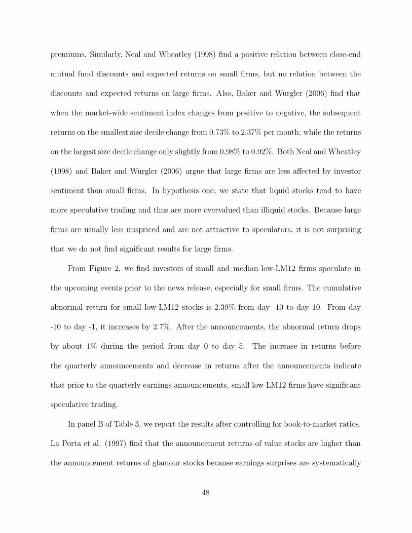
premiums. Similarly, Neal and Wheatley (1998) find a positive relation between close-end

mutual fund discounts and expected returns on small firms, but no relation between the

discounts and expected returns on large firms. Also, Baker and Wurgler (2006) find that

when the market-wide sentiment index changes from positive to negative, the subsequent

returns on the smallest size decile change from 0.73% to 2.37% per month; while the returns

on the largest size decile change only slightly from 0.98% to 0.92%. Both Neal and Wheatley

(1998) and Baker and Wurgler (2006) argue that large firms are less affected by investor

sentiment than small firms. In hypothesis one, we state that liquid stocks tend to have

more speculative trading and thus are more overvalued than illiquid stocks. Because large

firms are usually less mispriced and are not attractive to speculators, it is not surprising

that we do not find significant results for large firms.

From Figure 2, we find investors of small and median low-LM12 firms speculate in

the upcoming events prior to the news release, especially for small firms. The cumulative

abnormal return for small low-LM12 stocks is 2.39% from day -10 to day 10. From day

-10 to day -1, it increases by 2.7%. After the announcements, the abnormal return drops

by about 1% during the period from day 0 to day 5. The increase in returns before

the quarterly announcements and decrease in returns after the announcements indicate

that prior to the quarterly earnings announcements, small low-LM12 firms have significant

speculative trading.

In panel B of Table 3, we report the results after controlling for book-to-market ratios.

La Porta et al. (1997) find that the announcement returns of value stocks are higher than

the announcement returns of glamour stocks because earnings surprises are systematically

48

more positive for value stocks. Lee and Swaminathan (2000) also provide evidences that

the analysts’ growth forecasts for value stocks are more pessimistic than glamour stocks,

which results in future upward revision of growth forecasts and significant positive returns

of future earnings announcements. In Table 1, we show that low-LM12 stocks tend to be

growth stocks and high-LM12 stocks tend to be value stocks. To see whether our results

are driven by the effect of different book-to-market ratios, we divide our sample into 3

groups, growth, neutral, and value stocks, and test our hypothesis within each group.

Our results show that the differences of abnormal returns between high-LM12 stocks

and low-LM12 stocks are all significant positive in all 3 book-to-market groups right after

the announcements. The difference of cumulative abnormal returns between high-LM12

and low-LM12 stocks from day 0 to day 2 is 0.78% for growth stocks and 1.21% for value

stocks. From Figure 3, we find that low-LM12 growth stocks and low-LM12 value stocks

tend to have speculative trading before quarterly earnings announcements, which supports

that liquid stocks do have the bundle of salient characteristics that attract speculative

investors. The effect is more strong for low-LM12 growth stocks than for low-LM12 value

stocks, which is consistent with Baker and Wurgler (2006), who argue that growth stocks

are affected by investors’ speculative demand more than value stocks.

5.2.2 Control for Misperceptions of Future Earnings

Prior studies show that the return around earnings announcements is related to in-

vestors’ misperceptions of future earnings. La Porta (1996) documents that analysts’ esti-

mates of long-term growth show systematic errors. He finds that the one-year raw return

of high expected growth stocks is 20% lower than that of low expected growth stocks.

49

0

0.005

0.01

0.015

0.02

0.025

0.03

0.035

0.04

-10 -8 -6 -4 -2 0 2 4 6 8 10

Relative day

Growth, Low LM12 Growth, Median LM12 Growth, High LM12

Neutral, Low LM12 Neutral, Median LM12 Neutral, High LM12

Value, Low LM12 Value, Median LM12 Value, High LM12

Figure 3: Cumulative Abnormal Return during Quarterly Earnings Announcement Period: Control forBook-to-Market

This figure shows the cumulative abnormal return during quarterly earnings announcement periods after controlling for book-to-market. Sample includes quarterlyannouncements of firms listed on NYSE/AMEX/NASDAQ from 1982 to 2004. The abnormal volume is calculated from Fama and French 3-factor model. The cumulativeabnormal return is the sum of abnormal volume since day −10.

50

Furthermore, the excess return of earnings announcements is significant negative for high

expected growth stocks and positive for low expected growth stocks. He concludes that

analysts’ growth forecasts are too extreme so that following the earnings announcements,

analysts and investors both correct the biased forecasts. Lee and Swaminathan (2000) also

find that trading volume seems to provide information about investors’ misperceptions of

future earnings. Analysts are more optimistic for the future performance of high volume

stocks and provide higher long-term growth forecasts for high volume stocks than for low

volume stocks. However, low volume firms experience significantly better future operating

performance (measured by ROE). Because investors and analysts are too optimistic about

future earnings growth of high volume firms, they would revise their misperceptions during

the subsequent quarterly earnings announcements. As a result, high volume firms have

lower announcement returns than low volume firms.

This study differs from Lee and Swaminathan (2000) in that we focus on the effect of

overconfident investors’ speculative trading on the return of quarterly earnings announce-

ments, rather than the effect of investors’ misperceptions of future earnings. Due to short-

sale constraints, only overconfident investors whose valuation of a stock is higher than the

firm’s fundamental value buy the stock and reflect their opinions in the market. Therefore,

even if on average investors and analysts correctly forecast future earnings (that is, investors

do not have misperceptions of future earnings), the existence of the irrational overconfident

investors can still make liquid stocks overpriced. Because the returns of quarterly earnings

announcements capture both the effect of overconfident investors’ speculative trading on

stock prices and investors’ misperceptions of future earnings, in this subsection we examine

51

whether the speculative trading still affects the announcement returns after controlling for

investors’ misperceptions of future earnings.

We control two measures of investors’ misperceptions: errors of analysts’ earnings

forecasts and revisions of long-term growth forecasts. Both measures are obtained from

I/B/E/S summary database. I/B/E/S summary files compile analysts’ forecasts on the

third Thursday every month. If a quarterly announcement is made after the third Thursday

of a month, we define the forecast error as the actual earnings per share minus the consensus

forecast in the month of the announcement. If an announcement is made before the third

Thursday of a month, the forecast error is calculated as the actual earnings per share minus

analysts’ forecasts in the month before the announcement. For announcements made from

July year t to June year t+1, the forecast error is deflated by the stock price at end of June

year t. A positive (negative) forecast error indicates a positive (negative) information shock

of an announcement. The revision of long-term growth forecasts is defined as the growth

forecast right after the quarterly announcements minus the growth forecast right before the

quarterly announcements. If the earnings announcements contain information about future

earnings growth, after the announcement over-optimistic analysts should revise their growth

forecasts. Because we study the announcement returns during a very short event window

rather than the long-term performance, we only focus on the revision made right after

the earnings announcements. It is less likely that the 3-day event window of an earnings

announcement also reflect the analysts’ revision several months after the announcements.

Panel A of Table 4 and Figure 4 present the results after controlling for forecast errors.

We find for all three types of information shocks, the differences of abnormal returns

52

Table 4: Robustness Check for Earnings Announcement Effect on Stock Return: Control for Misperceptionsof Future Earnings

This table shows the abnormal returns during earnings announcement periods. Sample size varies with the intersection of CRSP and I/B/E/S Summary Database. Theabnormal return is calculated based on Fama and French 3-factor model. Panel A shows the results after controlling for the analyst forecast errors of the announcement.Forecast error is defined as the actual earnings per share (EPS) minus the last consensus of analysts forecast, deflated by the stock price at end of June in the previousyear. Firms are sorted based on the forecast error and are divided into 3 groups: positive shock (when the last consensus before the announcement is much lower thanthe actual EPS), Neutral shock (when the last consensus before the announcement is close to the actual EPS), and negative shock (when the last consensus before theannouncement is much higher than the actual EPS). Panel B controls for the revision of the long-term growth forecasts. Revisions of the long-term growth forecastsare defined as the estimates of long-term growth right after the announcement minus the estimates right before the announcement (Growth). Firms are divided into3 groups based on the direction of revisions: upward revision, no revision, and downward revision. In both panels, T-statistics are used to test the null hypothe-sis that the number is not different from zero. ***, **, and * indicate that a number is significantdifferent from zero at 1%, 5%, and 10%, respectively, from a two-tailed T test.

Panel A: Control for forecast errorPositive Shock Neutral Shock Negative Shock

Low High High Low High High Low High HighLM12

MedianLM12 −Low LM12

MedianLM12 −Low LM12

MedianLM12 −Low

# OBS 28829 21317 7214 35009 23171 4436 27143 22178 7507(-10, -2) 1.59%∗∗∗ 1.18%∗∗∗ 1.68%∗∗∗ 0.09% 0.58%∗∗∗ 0.22%∗∗∗ 0.63%∗∗∗ 0.05% -0.67∗∗∗% -0.62%∗∗∗ 0.04% 0.71%∗∗∗

-1 0.54%∗∗∗ 0.41%∗∗∗ 0.51%∗∗∗ -0.02% 0.14%∗∗∗ 0.09%∗∗∗ 0.13%∗∗ -0.01% -0.17%∗∗∗ -0.10%∗∗ 0.08% 0.24%∗∗∗

0 1.05%∗∗∗ 1.09%∗∗∗ 1.64%∗∗∗ 0.59%∗∗∗ 0.08%∗∗∗ 0.14%∗∗∗ 0.40%∗∗∗ 0.32%∗∗∗ -1.06%∗∗∗ -0.76%∗∗∗ -0.69%∗∗∗ 0.37%∗∗∗

1 0.59%∗∗∗ 0.64%∗∗∗ 0.67%∗∗∗ 0.08% 0.02% 0.07%∗∗∗ 0.14%∗∗ 0.13%∗ -1.00%∗∗∗ -0.52%∗∗∗ -0.41%∗∗∗ 0.59%∗∗∗

(2, 10) 0.27%∗∗∗ 0.74%∗∗∗ 0.89%∗∗∗ 0.62%∗∗∗ 0.15%∗∗∗ 0.30%∗∗∗ 0.41%∗∗∗ 0.25%∗ 0.02% -0.08% 0.07% 0.05%(0, 2) 1.68%∗∗∗ 1.87%∗∗∗ 2.49%∗∗∗ 0.81%∗∗∗ 0.09%∗∗ 0.24%∗∗∗ 0.55%∗∗∗ 0.46%∗∗∗ -2.13%∗∗∗ -1.34%∗∗∗ -1.14%∗∗∗ 0.99%∗∗∗

Error 0.0130∗∗∗ 0.0090∗∗∗ 0.0208∗∗ 0.0078 0.0001∗∗∗ 0.0001∗∗∗ 0.0001∗∗∗ 0.0000∗∗∗ -0.0559∗∗∗ -0.0427∗∗∗ -0.0364∗∗∗ 0.0195

Panel B: Control for revision of long-term growth

Downward Revision No Revision Upward RevisionLow High High Low High High Low High High

LM12Median

LM12 −Low LM12Median

LM12 −Low LM12Median

LM12 −Low

# OBS 24191 11879 1485 41068 35915 9840 17621 9164 763(-10, -2) 0.13%∗ -0.17%∗∗ 0.35% 0.22% 0.63%∗∗∗ 0.22%∗∗∗ 0.75%∗∗∗ 0.13% 0.70%∗∗∗ 0.33%∗∗∗ 1.03%∗∗∗ 0.33%

-1 0.08%∗∗∗ 0.12%∗∗ 0.02% -0.05% 0.20%∗∗∗ 0.10%∗∗∗ 0.28%∗∗∗ 0.08% 0.24%∗∗∗ 0.09%∗∗∗ 0.34%∗∗ 0.10%0 -0.10%∗∗∗ -0.04% 0.12% 0.21% 0.06%∗∗ 0.19%∗∗∗ 0.42%∗∗∗ 0.36%∗∗∗ 0.30%∗∗∗ 0.31%∗∗∗ 1.09%∗∗∗ 0.78%∗∗∗

1 -0.26%∗∗∗ -0.03% 0.05% 0.31% -0.10%∗∗∗ 0.05%∗∗ 0.09%∗ 0.19%∗∗∗ 0.28%∗∗∗ 0.27%∗∗∗ 0.46%∗∗ 0.18%(2, 10) 0.22%∗∗∗ 0.20%∗∗∗ 0.02% -0.20%∗∗ 0.15%∗∗∗ 0.31%∗∗∗ 0.52%∗∗∗ 0.37%∗∗∗ 0.25%∗∗∗ 0.53%∗∗∗ 0.60%∗ 0.35%

(0, 2) -0.33%∗∗∗ -0.03% 0.09% 0.41%∗ -0.07% 0.27%∗∗∗ 0.62%∗∗∗ 0.69%∗∗∗ 0.64%∗∗∗ 0.70%∗∗∗ 1.78%∗∗∗ 1.14%∗∗∗

∆Growth -1.63%∗∗∗ -1.48%∗∗∗ -3.21%∗∗∗ -1.58%∗∗∗ 0.00% 0.00% 0.00% 0.00% 1.42%∗∗∗ 1.36%∗∗∗ 3.00%∗∗∗ 1.58%∗∗∗

Growth 19.83% 15.42% 18.13% -1.70%∗∗∗ 19.42% 15.27% 16.03% -3.39%∗∗∗ 17.31% 13.43% 15.23% -2.08%∗∗∗

53

-0.04

-0.03

-0.02

-0.01

0

0.01

0.02

0.03

0.04

0.05

0.06

-10 -8 -6 -4 -2 0 2 4 6 8 10

Relative day

Postive shock, low LM12 Postive shock, median LM12 Postive shock, high LM12

Neutral shock, low LM12 Neutral shock, median LM12 Neutral shock, high LM12

Negative shock, low LM12 Negative shock, median LM12 Negative shock, high LM12

Figure 4: Cumulative Abnormal Return during Quarterly Earnings Announcement Period: Control forForecast Error

This figure shows the cumulative abnormal return during quarterly earnings announcement periods after controlling for analysts forecast error. Sample includes quarterlyannouncements of firms listed on NYSE/AMEX/NASDAQ from 1984 to 2004. The abnormal return is calculated from Fama and French 3-factor model. The cumulativeabnormal return is the sum of abnormal return since day −10. Positive (negative) shock is the announcement when the actual EPS is much higher (lower) than analysts’forecast.

54

between high-LM12 groups and low-LM12 groups are all significant during the period

(0, 2). The effect is more pronounced for announcements with negative shocks than for

announcements with positive or neutral shocks. However, after investigating the magnitude

of forecast errors, we find that analysts tend to be less optimistic for high-LM12 stocks

than for low-LM12 stocks, especially for negative events. In positive events, analysts, on

average, underestimate the earnings per share by 1.30 percent of stock prices for low-

LM12 stocks and by 2.08 percent for high-LM12 stocks. Similarly, in negative events,

they overestimate earnings by 5.59 percent of stock prices for low-LM12 stocks and by

3.64 percent for high-LM12 stocks. Because analysts’ forecasts before the announcements

are more optimistic for low-LM12 stocks than for high-LM12 stocks, the lower abnormal

returns for low-LM12 stocks may also result from analysts’ biased estimates. Although

our results may be partially driven by the analysts’ optimism about low-LM12 stocks, we

believe speculative trading as reflected in LM12 also has significant effects on the abnormal

returns. The difference of forecast errors between high-LM12 and low-LM12 stocks is not

significant in both of the positive events and negative events. In the neutral events, the

difference is significant statistically at 1% level but not significant economically because

its magnitude is less than 0.01% of stock prices. Considering that the abnormal returns

between high-LM12 and low-LM12 stocks are all significant at 1% in all three types of

events, we think that the results are unlikely to be caused solely by analysts’ forecast

errors.

In panel B of Table 4 and Figure 5 we report the results after controlling for the

revisions of growth forecasts. The total number of announcements is only 151,926 because

55

-0.005

0

0.005

0.01

0.015

0.02

0.025

0.03

0.035

0.04

-10 -8 -6 -4 -2 0 2 4 6 8 10

Relative day

Downward revision, Low LM12 Downward revision, Median LM12 Downward revision, High LM12

No revision, Low LM12 No revision, Median LM12 No revision, High LM12

Upward revision, Low LM12 Upward revision, Median LM12 Upward revision, High LM12

Figure 5: Cumulative Abnormal Return during Quarterly Earnings Announcement Period: Control forGrowth Revision

This figure shows the cumulative abnormal return during quarterly earnings announcement periods after controlling for growth revision. Sample includes quarterlyannouncements of firms listed on NYSE/AMEX/NASDAQ from 1984 to 2004. The abnormal return is calculated from Fama and French 3-factor model. The cumulativeabnormal return is the sum of abnormal return since day -10. Growth revision is the difference between analysts’ long-term growth forecasts right before and after theannouncement.

56

there are many missing value of analysts’ growth forecasts in I/B/E/S. Although the long-

term growth forecasts right before the announcements for low-LM12 stocks are significant

higher than the forecasts of high-LM12 stocks (by 1.70% for announcements with downward

revisions, 3.39%for announcements with no revisions, and by 2.08% for announcements with

upward revisions), the higher growth forecasts for low-LM12 stocks do not necessarily mean

that analysts are more over-optimistic for low-LM12 stocks than for high-LM12 stocks. For

both low-LM12 and high-LM12 stocks, downward revisions occur more frequently than the

upward revisions. Among all 151,926 announcements, 82,880 announcements are from low-

LM12 firms. About 21.26% of them receive upward revisions and 29.19% receive downward

revisions. There are 12,088 announcements from high-LM12 firms. 12.28% of them get

downward revisions and 6.30% obtain upward revisions. Therefore, in our sample, high-

LM12 stocks still receive many downward revisions and low-LM12 stocks also get many

upward revisions. Furthermore, the magnitude of revisions for high-LM12 stocks are larger

than that for low-LM12 stocks, irrespective to the direction of revisions. Based on the

directions and magnitude of growth revisions, we do not observe analysts are more over-

optimistic about future earnings growth for low-LM12 stocks than for high-LM12 stocks.

Because the abnormal returns for the announcements with downward revisions and the

announcements with upward revisions also reflect the effect of changes of growth forecasts,

we focus on the announcements without any revision. Among the 151,926 announcements,

more than 50% do not have any revision of long-term growth forecasts. The differences of

cumulative abnormal returns between high-LM12 stocks and low-LM12 stocks during the

event period (0, 2) is 0.69% and is significant at 1% level.

57

Our results in this subsection indicate that the differences of abnormal returns be-

tween high-LM12 and low-LM12 stocks do not solely result from investors’ misperceptions

of future earnings. Although analysts’ earnings forecasts are more optimistic for low-LM12

stocks, the differences of forecast errors between high-LM12 and low-LM12 stocks are not

significant for positive and negative events. Investigating the revisions of long-term growth

forecasts, we find that both high-LM12 and low-LM12 stocks receive more downward re-

visions than upward revisions right after quarterly announcements and that analysts are

not much more over-optimistic about future earnings growth for low-LM12 stocks than for

high-LM12 stocks. The fact that our results hold well after controlling for investors’ mis-

perceptions suggests that the overconfident investors’ speculative trading does affect stock

prices.

5.2.3 Control for Information Available, Dispersion in Opinions, and Informa-tiveness of Announcements

In this subsection, we do three robustness tests. The first robustness test controls for

information available to investors. We use the number of analysts following to measure

information available. Firms with more analysts following usually have more information

available to investors. The valuation of these firms is less subjective and investors may

have more accurate earnings forecasts. In Table 1, we show that high-LM12 firms are

usually low-following firms and low-LM12 firms are usually high-following firms. To rule

out the possibility that our results are affected by different amount of information available

to investors between high-LM12 and low-LM12 firms, we control for the number of analysts

following and redo our tests.

58

Panel A of Table 5 and Figure 6 provide the results after controlling for the number of

analysts following. There are 105,616 announcements from low-LM12 firms. Among these

announcements, 34.6% have low analysts following and 37.6% have high analysts following.

For the 58,328 announcements from high-LM12 firms, only 0.23% receive high analysts

coverage. 95.6% of high-LM12 firms receive low analysts following. For announcements

with low and median analysts following, our hypothesis hold well. High-LM12 stocks earn

significant larger abnormal returns than low-LM12 stocks. However, for announcements

with high analysts following, the result is not significant. The insignificant result may

be partially driven by the small sample size for high-LM12 high-following firms. Another

possibility is that firms with high analysts following but high LM12 may suffer firm-specific

problems such as financial distress. Although they are followed by many analysts, the

specific firm problems influence investors’ willingness to trade and may also affect the

announcement returns.

From Figure 6, we find that low-LM12 low-following stocks tend to have speculative

trading before quarterly earnings announcements. Although the information available for

these firms is limited, investors still trade frequently. If we resort to an explanation of

irrational behavior, we can attribute this phenomenon to the demand of propensity to

speculate proposed by Baker and Wurgler (2006). Firms with low analysts following are

difficult to price. Because their valuation is very subjective, investors have a wide spectrum

of valuations, from much too low to much too high. When the trading of these stocks are

very active, the market is dominated by irrational investors and thus the speculative trading

for low-following but low-LM12 stocks is prevalent.

59

Table 5: Robustness Check for Earnings Announcement Effect on Stock Return: Control for InformationAvailable, Dispersion in Opinions, and Informativeness of Announcements

This table shows the abnormal returns during earnings announcement periods. Sample varies with the intersection of CRSP and I/B/E/S Summary Database. Theabnormal return is calculated based on Fama and French 3-factor model. Panel A controls for the number of analyst following. Number of analyst following is defined asthe number of estimates in I/B/E/S right before the announcements. If the number of analyst following is not available in I/B/E/S, we set it zero. 9 groups are formedbased on two independent sorts of the number of analyst following and LM12. Panel B controls for the analysts forecast dispersion. Forecast dispersion is defined as thestandard deviation of analysts earnings estimates right before the announcements. Only announcements which have at least two analysts following are included in oursample. 9 groups are formed based on the two independent sorts of the analysts forecast dispersion and LM12. Panel C controls for the changes of return volatility afterannouncements. The changes of return volatility is defined as the standard deviation of stock return during the period (11, 40) minus the standard deviation of stockreturn during the period (-40, -11). In all panels, T-statistics are used to test the null hypothesis that the number is not different from zero. ***, **, and * indicate that anumber is significant different from zero at 1%, 5%, and 10%, respectively, from a two-tailed T test.

Panel A: Control for analyst followingLow Following Median Following High Following

Low High High Low High High Low High HighLM12

MedianLM12 −Low LM12

MedianLM12 −Low LM12

MedianLM12 −Low

# OBS 36548 61408 55768 29397 20902 2423 39671 13855 137

(-10, -2) 0.72%∗∗∗ 0.63%∗∗∗ 1.28%∗∗∗ 0.56%∗∗∗ 0.61%∗∗∗ 0.12%∗ 0.27% -0.34% 0.34%∗∗∗ -0.09% 0.38% 0.04%-1 0.21%∗∗∗ 0.23%∗∗∗ 0.31%∗∗∗ 0.09%∗∗ 0.19%∗∗∗ 0.10%∗∗∗ 0.36%∗∗∗ 0.17%∗∗ 0.14%∗∗∗ 0.01% -0.49% -0.63%∗

0 -0.14%∗∗∗ 0.15%∗∗∗ 0.59%∗∗∗ 0.73%∗∗∗ 0.07%∗ 0.20%∗∗∗ 0.24%∗∗ 0.17% 0.10%∗∗∗ 0.08%∗∗ 0.16% 0.05%1 -0.41%∗∗∗ -0.03% 0.18%∗∗∗ 0.59%∗∗∗ -0.13%∗∗∗ 0.07%∗∗ 0.10% 0.23%∗∗ 0.05%∗ 0.11%∗∗∗ -0.06% -0.10%

(2, 10) 0.14%∗∗ 0.41%∗∗∗ 0.89%∗∗∗ 0.75%∗∗∗ 0.13%∗ 0.28%∗∗∗ 0.53%∗∗∗ 0.41%∗∗ 0.18%∗∗∗ 0.30%∗∗∗ -0.06% -0.24%(0, 2) -0.61%∗∗∗ 0.13%∗∗∗ 0.91%∗∗∗ 1.52%∗∗∗ -0.08% 0.33%∗∗∗ 0.52%∗∗∗ 0.60%∗∗∗ 0.17%∗∗∗ 0.26%∗∗∗ 0.11% -0.06%

Panel B: Control for forecast dispersion

Low Dispersion Median Dispersion High DispersionLow High High Low High High Low High High

LM12Median

LM12 −Low LM12Median

LM12 −Low LM12Median

LM12 −Low

# OBS 42153 28635 4891 14035 8203 956 24686 12706 1743(-10, -2) 0.76%∗∗∗ 0.23%∗∗∗ 0.75%∗∗∗ -0.01% 0.26%∗∗∗ 0.00% 0.61%∗ 0.35% 0.10% -0.11% 0.17% 0.07%

-1 0.23%∗∗∗ 0.15%∗∗∗ 0.27%∗∗∗ 0.04% 0.12%∗∗∗ 0.01% -0.05% -0.17% 0.10%∗∗∗ 0.01% 0.30%∗∗∗ 0.20%∗

0 0.15%∗∗∗ 0.20%∗∗∗ 0.51%∗∗∗ 0.36%∗∗∗ 0.04% 0.17%∗∗∗ 0.26% 0.23% -0.08%∗∗ 0.05% 0.20% 0.28%∗

1 0.03% 0.09%∗∗∗ 0.12%∗ 0.09% -0.08%∗ 0.08%∗ 0.12% 0.20% -0.23%∗∗∗ 0.00% 0.01% 0.24%∗

(2, 10) 0.24%∗∗∗ 0.38%∗∗∗ 0.44%∗∗∗ 0.20% 0.32%∗∗∗ 0.19%∗∗ 0.80%∗∗ 0.47% -0.08% 0.21%∗∗ 0.33% 0.41%

(0, 2) 0.19%∗∗∗ 0.33%∗∗∗ 0.70%∗∗∗ 0.51%∗∗∗ -0.02% 0.27%∗∗∗ 0.58%∗∗ 0.60%∗∗ -0.35%∗∗∗ 0.15%∗∗ 0.15% 0.50%∗∗

60

Table 5 continued

Panel C: Control for changes of return volatilityDecrease in Volatility Little Change in Volatility Increase in Volatility

Low High High Low High High Low High HighLM12

MedianLM12 −Low LM12

MedianLM12 −Low LM12

MedianLM12 −Low

# OBS 35002 28711 20017 36166 36578 16260 33282 29898 20944

(-10, -2) 1.16%∗∗∗ 0.97%∗∗∗ 2.05%∗∗∗ 0.89%∗∗∗ 0.49%∗∗∗ 0.29%∗∗∗ 0.82%∗∗∗ 0.34%∗∗∗ -0.09% -0.02% 0.75%∗∗∗ 0.84%∗∗∗

-1 0.28%∗∗∗ 0.32%∗∗∗ 0.39%∗∗∗ 0.11%∗∗ 0.15%∗∗∗ 0.12%∗∗∗ 0.26%∗∗∗ 0.11%∗∗∗ 0.10%∗∗∗ 0.09%∗∗∗ 0.26%∗∗∗ 0.15%∗∗∗

0 0.15%∗∗∗ 0.27%∗∗∗ 0.80%∗∗∗ 0.65%∗∗∗ 0.13%∗∗∗ 0.18%∗∗∗ 0.56%∗∗∗ 0.42%∗∗∗ -0.25%∗∗∗ 0.00% 0.36%∗∗∗ 0.61%∗∗∗

1 -0.06%∗ 0.10%∗∗∗ 0.25%∗∗∗ 0.32%∗∗∗ 0.04% 0.05%∗∗ 0.19%∗∗∗ 0.16%∗∗∗ -0.45%∗∗∗ -0.11%∗∗∗ 0.11%∗∗ 0.56%∗∗∗

(2, 10) 0.48%∗∗∗ 0.58%∗∗∗ 1.26%∗∗∗ 0.79%∗∗∗ 0.38%∗∗∗ 0.44%∗∗∗ 0.57%∗∗∗ 0.19%∗∗ -0.41% 0.03% 0.67% 1.08%∗∗∗

(0, 2) 0.10%∗ 0.39%∗∗∗ 1.25%∗∗∗ 1.15%∗∗∗ 0.20%∗∗∗ 0.31%∗∗∗ 0.86%∗∗∗ 0.66%∗∗∗ -0.79%∗∗∗ -0.15%∗∗∗ 0.58%∗∗∗ 1.38%∗∗∗

61

-0.005

0

0.005

0.01

0.015

0.02

0.025

0.03

0.035

-10 -8 -6 -4 -2 0 2 4 6 8 10

Relative day

Low following, Low LM12 Low following, Median LM12 Low following, High LM12

Median following, Low LM12 Median following, Median LM12 Median following, High LM12

High following, Low LM12 High following, Median LM12 High following, High LM12

z

Figure 6: Cumulative Abnormal Return during Quarterly Earnings Announcement Period: Control forAnalysts Following

This figure shows the cumulative abnormal return during quarterly earnings announcement periods after controlling for number of analyst following. Sample includesquarterly announcements of firms listed on NYSE/AMEX/NASDAQ from 1982 to 2004. The abnormal return is calculated from Fama and French 3-factor model. Thecumulative abnormal return is the sum of abnormal return since day −10.

62

The second robustness test in this subsection controls for the dispersions in opinions

among investors. The dispersions in opinions affect stock returns when short-sale con-

straints exist. With short-sale constraints, investors with pessimistic views do not trade;

while optimistic investors buy stocks and reflect their opinions to the public. Therefore,

even if on average investors are rational, short-sale constraints may still result in overpric-

ing. The overpricing is more severe for stocks with larger dispersions in investors’ opinions.

Diether, Malloy, and Scherbina (2002) find that stocks with higher dispersions in analysts’

earnings forecasts tend to be more overvalued and earn lower future returns than otherwise

similar stocks. In Diether, Malloy, and Scherbina (2002), investors are rational and the

analysts’ forecast dispersion is a proxy of the dispersion in opinions.

On the other hand, Scheinkman and Xiong (2003) propose a model in which investors

are overconfident. In their model, due to short-sale constraints, investors who buy a stock

also obtain an option to sell it in the future. When the difference in beliefs is higher, an

overconfident investor expects that he can sell the stock to other overconfident investors

who are even more optimistic. As a result, the re-sale option embedded in the stock is

more valuable when the dispersion in opinions is higher. In their model, the overconfidence

results in differences of beliefs which in turn boosts speculative trading.

To see whether liquidity contains more information than analysts’ forecast disper-

sions, we control for dispersions in opinions. We get the forecast dispersion from I/B/E/S.

Because there should be at least two analysts’ forecasts for the calculation of forecast dis-

persions, we lose many observations of high-LM12 stocks which usually have, if any, only

one analyst following. The results are presented in panel B of Table 5 and Figure 7.

63

-0.005

0

0.005

0.01

0.015

0.02

0.025

-10 -8 -6 -4 -2 0 2 4 6 8 10

Relative day

Low Dispersion, Low LM12 Low Dispersion, Median] LM12 Low Dispersion, High LM12

Medain Dispersion, Low LM12 Medain Dispersion, Median] LM12 Medain Dispersion, High LM12

High Dispersion, Low LM12 High Dispersion, Median] LM12 HighDispersion, High LM12

Figure 7: Cumulative Abnormal Return during Quarterly Earnings Announcement Period: Control forForecast Dispersion

This figure shows the cumulative abnormal return during quarterly earnings announcement periods after controlling forecast dispersion. Sample includes quarterly an-nouncements of firms listed on NYSE/AMEX/NASDAQ from 1984 to 2004. The abnormal return is calculated from Fama and French 3-factor model. The cumulativeabnormal return is the sum of abnormal return since day -10. Forecast Dispersion is the standard deviation among all analysts forecasts right before the announcement.

64

Consistent with our first hypothesis, high-LM12 stocks have significant higher abnormal

returns than low-LM12 stocks in all 3 dispersion groups during the period (0, 2). Fur-

thermore, low-LM12 high-dispersion stocks have the lowest abnormal returns among all

dispersion-LM12 groups. This result shows that low-LM12 high-dispersion stocks show the

highest degree of overpricing so that after the announcements its return is the lowest. In-

vestigating the return path around the announcements in Figure 7, we find that low-LM12

high-dispersion stocks have positive abnormal returns before the announcements and neg-

ative abnormal returns after the announcements. If investors are rational and stocks are

overpriced before earnings announcements because of the large dispersions of opinion, we

should observe an increase in return before and a decrease in return after the announcements

for all three high dispersion groups. However, this pattern only exists for high-dispersion

low-LM12 stocks. This evidence is consistent with Scheinkman and Xiong (2003) which

shows that liquid stocks have higher differences in beliefs and more speculative trading

than illiquid stocks.

In the last test of this subsection, we use changes of return volatility to measure the

informativeness of announcements. The return volatility can be a proxy for the disagree-

ment of stock prices. If after the announcement, the return volatility does not change (that

is, the disagreement remains the same), the announcement may not be very informative. If

after the announcement, the return volatility decreases, the announcement is informative

because it mitigates the disagreement among different investors. On the contrary, if the

return volatility increases after the announcement, the announcement may convey surprises

which enlarge the disagreement. We define the changes of return volatility as the standard

65

deviation of stock returns during the period (11, 40) minus the standard deviation of stock

returns during the period (−40, −11)9. When the announcement is more informative, irra-

tional investors may have larger revision of their mispricing, which magnifies the difference

of abnormal returns between high-LM12 and low-LM12 stocks around quarterly earnings

announcements.

In Panel C of Table 5 and Figure 8, we provide the results after controlling the changes

of return volatility. In all 3 groups, high-LM12 stocks have significant higher abnormal re-

turns than low-LM12 stocks after the announcements. Furthermore, for low-LM12 stocks,

the abnormal returns during the period (0, 2) decrease from 0.20% for announcements

with little change in volatility to 0.10% for announcements with a decrease in volatility.

On the contrary, for high-LM12 stocks, the abnormal returns increase from 0.86% for an-

nouncements with little change in volatility to 1.25% for announcements with a decrease

in volatility. If the decrease in volatility is a good news for investors, the return for the an-

nouncements with decrease in volatility should be higher than the return for the announce-

ments with little change in volatility. The fact that low-LM12 stocks with a decrease in

volatility show lower returns than low-LM12 stocks with little change in volatility support

the argument that overconfident investors correct their mispricing more for informative

announcements than for non-informative announcements.

For the announcements with an increase in volatility, the difference between high-

LM12 and low-LM12 stocks is the highest among three groups. For low-LM12 stocks,

9The results are similar when we define the changes of return volatility as the standard deviation ofstock returns during the period (11, 20) minus the standard deviation of stock returns during the period(−20, −11).

66

-0.02

-0.01

0

0.01

0.02

0.03

0.04

0.05

0.06

-10 -8 -6 -4 -2 0 2 4 6 8 10

Relative day

Decrease in volatility, Low LM12 Decrease in volatility, Median LM12 Decrease in volatility, High LM12

Little change in volatility, Low LM12 Little change, Median LM12 Little change, High LM12

Increase in volatility, Low LM12 Increase in volatility, Median LM12 Increase in volatility, High LM12

Figure 8: Cumulative Abnormal Return during Quarterly Earnings Announcement Period: Control forChange in Volatility

This figure shows the cumulative abnormal return during quarterly earnings announcement periods after controlling forecast dispersion. Sample includes quarterly an-nouncements of firms listed on NYSE/AMEX/NASDAQ from 1984 to 2004. The abnormal return is calculated from Fama and French 3-factor model. The cumulativeabnormal return is the sum of abnormal return since day -10. The changes of return volatility is defined as the standard deviation of stock return during the period (11,40) minus the standard deviation of stock return during the period (−40, −11).

67

the abnormal returns change from 0.20% for announcements with little change in volatility

to -0.79% for announcements with an increase in volatility. For high-LM12 stocks, the

abnormal returns decrease from 0.86% for announcements with little change in volatility to

0.58% for announcements with an increase in volatility. Apparently, investors of low-LM12

stocks are more surprised at the increase in volatility than investors of high-LM12 stocks.

If we view the increase in volatility as a bad news, low-LM12 stocks is more sensitive to bad

news than high-LM12 stocks. A possible explanation is that after a bad news is released,

overconfident investors are shocked and may correct their mispricing more thoroughly.

5.2.4 Control for Changes of Future Liquidity

Liquid (illiquid) stocks are usually more likely to experience a liquidity deterioration

(improvement) in the future. If the earnings announcements contain information which

affects the future liquidity of a stock, the announcement effects may be affected by the in-

formation about changes of future liquidity. Hence, the low (high) announcement return of

low-LM12 (high-LM12) stocks may result from the information about liquidity downgrade

(upgrade) from the quarterly announcements. In this subsection, we control for changes of

future liquidity after the announcements. Because the changes of liquidity may be affected

by other events which occur after the earnings announcements, rather than by the infor-

mation conveyed by earnings announcements per se, an upgrade (downgrade) of liquidity

in the future is not necessarily related to a higher (lower) announcement returns.

We define the upgrade/downgrade of liquidity based on the movement of stocks from

one LM12 decile to another. For any quarterly announcement made by a firm between

July year t and June year t + 1, if that firm moves from a lower (higher) LM12 decile

68

to a higher (lower) LM12 decile from the end of June year t to June year t + 1, we assign

it into the liquidity downgrade (upgrade) group. The results are shown in Table 6 and the

graphical summaries are presented in Figure 9. Again high-LM12 stocks still earn higher

abnormal returns than low-LM12 stocks during the period (0, 2) for all liquidity-downgrade,

liquidity-upgrade, and liquidity-same groups. Furthermore, for both high-LM12 and low-

LM12 stocks, we find, in general, the abnormal returns in downgrade groups are lower

than their counterparts in upgrade groups. This indicates that the earnings announcements

may convey information about changes of future liquidity. Investors may either perceive the

future changes and require a higher (lower) rate of return for liquidity-downgrade (upgrade)

stocks, or be discouraged (stimulated) by the information content of the announcements

and trade less (more) frequently after the announcements. From Figure 9, we find low-LM12

stocks with future liquidity downgrade tend to have more speculative trading before the

announcements. A possible explanation is that investors revise not only their mispricing but

also their trading activities for low-LM12 stocks after the announcements. Therefore, stocks

with more speculative trading prior to the announcements experience liquidity downgrade

after the announcements.

5.2.5 Control for Changes in Risk

Risk potentially may affect the abnormal returns around quarterly earnings announce-

ments. Because the information available for high-LM12 stocks is less than that for low-

LM12 stocks, the uncertainty of future performance for high-LM12 stocks may be higher

than that of low-LM12 stocks. Therefore, the earnings releases for high-LM12 stocks may

resolve investors’ concern about risk more significantly than the announcements of

69

Table 6: Robustness Check for Earnings Announcement Effect on Stock Return: Control for Change ofLiquidity

This table shows the abnormal returns during earnings announcement periods. The abnormal return is calculated based on Fama and French 3-factor model. In June yeart − 1 and in June year t, all stocks are grouped into ten portfolios based on the sort of LM12. The breakpoints are calculated from all stocks listed in NYSE, AMEX, andNASDAQ. If, from Jun. year t − 1 to Jun. year t, firms move from a lower LM12 decile to a higher LM12 decile, they are assigned to the “liquidity upgrade” group. Iffrom year t − 1 to year t, firms remain in the same decile, they are assigned to the “liquidity same” group. If from year t − 1 to year t, firms move from a higher LM12decile to a lower LM12 decile, they are assigned to the “liquidity downgrade”. Then at the end June of each year, all firms are assigned into 9 groups based on LM12 andchanges of liquidity. The T-statistics are used to test the null hypothesis that the number is not different from zero. ***, **, and * indicate that a number is significantdifferent from zero at 1%, 5%, and 10%, respectively, from a two-tailed T test.

Liquidity Downgrade Liquidity Same Liquidity UpgradeLow High High Low High High Low High High

LM12Median

LM12 −Low LM12Median

LM12 −Low LM12Median

LM12 −Low# OBS 38190 28635 12003 47303 34867 27840 15913 28750 14521(-10, -2) 0.38%∗∗∗ 0.31%∗∗∗ 0.90%∗∗∗ 0.52%∗∗∗ 0.55%∗∗∗ 0.16%∗∗∗ 1.05%∗∗∗ 0.49%∗∗∗ 0.77%∗∗∗ 0.72%∗∗∗ 1.67%∗∗∗ 0.90%∗∗∗

-1 0.17%∗∗∗ 0.18%∗∗∗ 0.21%∗∗∗ 0.03% 0.15%∗∗∗ 0.09%∗∗∗ 0.27%∗∗∗ 0.11%∗∗∗ 0.21%∗∗∗ 0.25%∗∗∗ 0.48%∗∗∗ 0.27%∗∗∗

0 0.03% 0.15%∗∗∗ 0.41%∗∗∗ 0.38%∗∗∗ 0.04% 0.13%∗∗∗ 0.60%∗∗∗ 0.56%∗∗∗ 0.00% 0.16%∗∗∗ 0.78%∗∗∗ 0.78%∗∗∗

1 -0.23%∗∗∗ 0.04% 0.21%∗∗∗ 0.44%∗∗∗ -0.12%∗∗∗ 0.05%∗∗ 0.25%∗∗∗ 0.37%∗∗∗ 0.13%∗∗ -0.01% 0.09%∗ -0.04%(2, 10) -0.11%∗ 0.32%∗∗∗ 0.59%∗∗∗ 0.71%∗∗∗ 0.22%∗∗∗ 0.26%∗∗∗ 0.94%∗∗∗ 0.72%∗∗∗ 0.63%∗∗∗ 0.43%∗∗∗ 0.73%∗∗∗ 0.10%

(0, 2) -0.26%∗∗∗ 0.21%∗∗∗ 0.71%∗∗∗ 0.97%∗∗∗ -0.08%∗ 0.22%∗∗∗ 1.04%∗∗∗ 1.13%∗∗∗ 0.22%∗∗ 0.14%∗∗∗ 0.97%∗∗∗ 0.74%∗∗∗

70

-0.005

0

0.005

0.01

0.015

0.02

0.025

0.03

0.035

0.04

-10 -8 -6 -4 -2 0 2 4 6 8 10

Relative day

Liquidity downgrade, Low LM12 Liquidity downgrade, Median LM12 Liquidity downgrade, High LM12

Liquidity same, Low LM12 Liquidity same, Median LM12 Liquidity same, High LM12

Liquidity upgrade, Low LM12 Liquidity upgrade, Median LM12 Liquidity upgrade, High LM12

Figure 9: Cumulative Abnormal Return during Quarterly Earnings Announcement Period: Control forChanges of Liquidity

This figure shows the cumulative abnormal return during quarterly earnings announcement periods. Sample includes quarterly announcements of firms listed onNYSE/AMEX/NASDAQ from 1982 to 2004. The abnormal return is calculated from Fama and French 3-factor model. The cumulative abnormal return is the sumof abnormal return since day −10. Up (Down) indicates that the liquidity of stocks increase (decrease) from June year t − 1 to June year t.

71

low-LM12 stocks. To rule out the possibility that our results are attributed to changes in

risk caused by earnings announcements, in this subsection, we control for changes in risk in

our analysis. We run Fama and French 3-factor model for both period (-40, -11) and period

(11, 40), compare the factor loadings between these two periods, and divide our sample into

three groups: decrease in risk, little change in risk, and increase in risk. Since we cannot

know whether changes in risk are driven by information from earnings announcements or

not, the changes in risk may not be associated with the differences of announcement returns.

The results are shown in Table 7 and the graphical summaries are presented in Figure 10,

Figure 11, and Figure 12. After controlling for changes in risk, the abnormal returns for

high-LM12 stocks are still significant higher than that of low-LM12 stocks during the period

(0, 2). However, the abnormal returns of announcements with a decrease in risk are not

necessarily higher than the returns of announcements with an increase in risk. Our results

do not show that returns of earnings announcements reflect changes in future risk. We

conjecture that on average the changes in risk are not large enough to affect announcement

returns. Thus, announcements with a future increase (decrease) in risk may have certain

characteristics which lead to high (low) announcement returns.

5.2.6 Use Market-Adjusted Return, Use Only NYSE/AMEX Stocks, and UseOnly Announcements with Trade on Day -2

In this subsection, we do three robustness checks. First, in previous analysis, we

calculate the abnormal return from Fama-French 3-factor model.To rule out the possibility

that our results are driven by this specific asset pricing model, we calculate the market-

adjusted returns (raw stock return minus value-weighted index of NYSE, AMEX, and

72

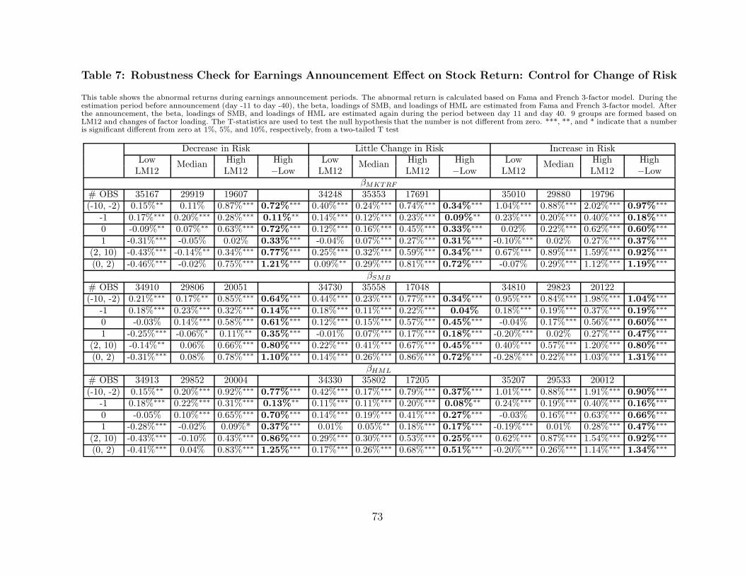
Table 7: Robustness Check for Earnings Announcement Effect on Stock Return: Control for Change of Risk

This table shows the abnormal returns during earnings announcement periods. The abnormal return is calculated based on Fama and French 3-factor model. During theestimation period before announcement (day -11 to day -40), the beta, loadings of SMB, and loadings of HML are estimated from Fama and French 3-factor model. Afterthe announcement, the beta, loadings of SMB, and loadings of HML are estimated again during the period between day 11 and day 40. 9 groups are formed based onLM12 and changes of factor loading. The T-statistics are used to test the null hypothesis that the number is not different from zero. ***, **, and * indicate that a numberis significant different from zero at 1%, 5%, and 10%, respectively, from a two-tailed T test

Decrease in Risk Little Change in Risk Increase in RiskLow High High Low High High Low High High

LM12Median

LM12 −Low LM12Median

LM12 −Low LM12Median

LM12 −LowβMKTRF

# OBS 35167 29919 19607 34248 35353 17691 35010 29880 19796(-10, -2) 0.15%∗∗ 0.11% 0.87%∗∗∗ 0.72%∗∗∗ 0.40%∗∗∗ 0.24%∗∗∗ 0.74%∗∗∗ 0.34%∗∗∗ 1.04%∗∗∗ 0.88%∗∗∗ 2.02%∗∗∗ 0.97%∗∗∗

-1 0.17%∗∗∗ 0.20%∗∗∗ 0.28%∗∗∗ 0.11%∗∗ 0.14%∗∗∗ 0.12%∗∗∗ 0.23%∗∗∗ 0.09%∗∗ 0.23%∗∗∗ 0.20%∗∗∗ 0.40%∗∗∗ 0.18%∗∗∗

0 -0.09%∗∗ 0.07%∗∗ 0.63%∗∗∗ 0.72%∗∗∗ 0.12%∗∗∗ 0.16%∗∗∗ 0.45%∗∗∗ 0.33%∗∗∗ 0.02% 0.22%∗∗∗ 0.62%∗∗∗ 0.60%∗∗∗

1 -0.31%∗∗∗ -0.05% 0.02% 0.33%∗∗∗ -0.04% 0.07%∗∗∗ 0.27%∗∗∗ 0.31%∗∗∗ -0.10%∗∗∗ 0.02% 0.27%∗∗∗ 0.37%∗∗∗

(2, 10) -0.43%∗∗∗ -0.14%∗∗ 0.34%∗∗∗ 0.77%∗∗∗ 0.25%∗∗∗ 0.32%∗∗∗ 0.59%∗∗∗ 0.34%∗∗∗ 0.67%∗∗∗ 0.89%∗∗∗ 1.59%∗∗∗ 0.92%∗∗∗

(0, 2) -0.46%∗∗∗ -0.02% 0.75%∗∗∗ 1.21%∗∗∗ 0.09%∗∗ 0.29%∗∗∗ 0.81%∗∗∗ 0.72%∗∗∗ -0.07% 0.29%∗∗∗ 1.12%∗∗∗ 1.19%∗∗∗

βSMB

# OBS 34910 29806 20051 34730 35558 17048 34810 29823 20122(-10, -2) 0.21%∗∗∗ 0.17%∗∗ 0.85%∗∗∗ 0.64%∗∗∗ 0.44%∗∗∗ 0.23%∗∗∗ 0.77%∗∗∗ 0.34%∗∗∗ 0.95%∗∗∗ 0.84%∗∗∗ 1.98%∗∗∗ 1.04%∗∗∗

-1 0.18%∗∗∗ 0.23%∗∗∗ 0.32%∗∗∗ 0.14%∗∗∗ 0.18%∗∗∗ 0.11%∗∗∗ 0.22%∗∗∗ 0.04% 0.18%∗∗∗ 0.19%∗∗∗ 0.37%∗∗∗ 0.19%∗∗∗

0 -0.03% 0.14%∗∗∗ 0.58%∗∗∗ 0.61%∗∗∗ 0.12%∗∗∗ 0.15%∗∗∗ 0.57%∗∗∗ 0.45%∗∗∗ -0.04% 0.17%∗∗∗ 0.56%∗∗∗ 0.60%∗∗∗

1 -0.25%∗∗∗ -0.06%∗ 0.11%∗∗ 0.35%∗∗∗ -0.01% 0.07%∗∗∗ 0.17%∗∗∗ 0.18%∗∗∗ -0.20%∗∗∗ 0.02% 0.27%∗∗∗ 0.47%∗∗∗

(2, 10) -0.14%∗∗ 0.06% 0.66%∗∗∗ 0.80%∗∗∗ 0.22%∗∗∗ 0.41%∗∗∗ 0.67%∗∗∗ 0.45%∗∗∗ 0.40%∗∗∗ 0.57%∗∗∗ 1.20%∗∗∗ 0.80%∗∗∗

(0, 2) -0.31%∗∗∗ 0.08% 0.78%∗∗∗ 1.10%∗∗∗ 0.14%∗∗∗ 0.26%∗∗∗ 0.86%∗∗∗ 0.72%∗∗∗ -0.28%∗∗∗ 0.22%∗∗∗ 1.03%∗∗∗ 1.31%∗∗∗

βHML

# OBS 34913 29852 20004 34330 35802 17205 35207 29533 20012

(-10, -2) 0.15%∗∗ 0.20%∗∗∗ 0.92%∗∗∗ 0.77%∗∗∗ 0.42%∗∗∗ 0.17%∗∗∗ 0.79%∗∗∗ 0.37%∗∗∗ 1.01%∗∗∗ 0.88%∗∗∗ 1.91%∗∗∗ 0.90%∗∗∗

-1 0.18%∗∗∗ 0.22%∗∗∗ 0.31%∗∗∗ 0.13%∗∗ 0.11%∗∗∗ 0.11%∗∗∗ 0.20%∗∗∗ 0.08%∗∗ 0.24%∗∗∗ 0.19%∗∗∗ 0.40%∗∗∗ 0.16%∗∗∗

0 -0.05% 0.10%∗∗∗ 0.65%∗∗∗ 0.70%∗∗∗ 0.14%∗∗∗ 0.19%∗∗∗ 0.41%∗∗∗ 0.27%∗∗∗ -0.03% 0.16%∗∗∗ 0.63%∗∗∗ 0.66%∗∗∗

1 -0.28%∗∗∗ -0.02% 0.09%* 0.37%∗∗∗ 0.01% 0.05%∗∗ 0.18%∗∗∗ 0.17%∗∗∗ -0.19%∗∗∗ 0.01% 0.28%∗∗∗ 0.47%∗∗∗

(2, 10) -0.43%∗∗∗ -0.10% 0.43%∗∗∗ 0.86%∗∗∗ 0.29%∗∗∗ 0.30%∗∗∗ 0.53%∗∗∗ 0.25%∗∗∗ 0.62%∗∗∗ 0.87%∗∗∗ 1.54%∗∗∗ 0.92%∗∗∗

(0, 2) -0.41%∗∗∗ 0.04% 0.83%∗∗∗ 1.25%∗∗∗ 0.17%∗∗∗ 0.26%∗∗∗ 0.68%∗∗∗ 0.51%∗∗∗ -0.20%∗∗∗ 0.26%∗∗∗ 1.14%∗∗∗ 1.34%∗∗∗

73

-0.01

0

0.01

0.02

0.03

0.04

0.05

0.06

-10 -8 -6 -4 -2 0 2 4 6 8 10

Relative day

Decrease in ristk, Low LM12 Decrease in ristk, Median LM12 Decrease in ristk, High LM12

Little change in ristk, Low LM12 Little change in ristk, Median LM12 Little change in ristk, High LM12

Increase in ristk, Low LM12 Increase in ristk, Median LM12 Increase in ristk, High LM12

Figure 10: Cumulative Abnormal Return during Quarterly Earnings Announcement Period: Control forChanges of βMKTRF

This figure shows the cumulative abnormal return during quarterly earnings announcement periods after controlling for changes of βMKTRF . Sample includes quarterlyannouncements of firms listed on NYSE/AMEX/NASDAQ from 1982 to 2004. The abnormal return is calculated from Fama and French 3-factor model. The cumulativeabnormal return is the sum of abnormal return since day −10. The changes of beta is defined as the difference between the beta during (−40, −11) and during (11, 40).

74

-0.005

0

0.005

0.01

0.015

0.02

0.025

0.03

0.035

0.04

0.045

0.05

-10 -8 -6 -4 -2 0 2 4 6 8 10

Relative day

Decrease in ristk, Low LM12 Decrease in ristk, Median LM12 Decrease in ristk, High LM12

Little change in ristk, Low LM12 Little change in ristk, Median LM12 Little change in ristk, High LM12

Increase in ristk, Low LM12 Increase in ristk, Median LM12 Increase in ristk, High LM12

Figure 11: Cumulative Abnormal Return during Quarterly Earnings Announcement Period: Control forChanges of βSMB

This figure shows the cumulative abnormal return during quarterly earnings announcement periods after controlling for changes of βSMB. Sample includes quarterlyannouncements of firms listed on NYSE/AMEX/NASDAQ from 1982 to 2004. The abnormal return is calculated from Fama and French 3-factor model. The cumulativeabnormal return is the sum of abnormal return since day −10. The changes of beta is defined as the difference between the beta during (−40, −11) and during (11, 40).

75

-0.01

0

0.01

0.02

0.03

0.04

0.05

0.06

-10 -8 -6 -4 -2 0 2 4 6 8 10

Relative day

Decrease in ristk, Low LM12 Decrease in ristk, Median LM12 Decrease in ristk, High LM12

Little change in ristk, Low LM12 Little change in ristk, Median LM12 Little change in ristk, High LM12

Increase in ristk, Low LM12 Increase in ristk, Median LM12 Increase in ristk, High LM12

Figure 12: Cumulative Abnormal Return during Quarterly Earnings Announcement Period: Control forChanges of βHML

This figure shows the cumulative abnormal return during quarterly earnings announcement periods after controlling for changes of βHML. Sample includes quarterlyannouncements of firms listed on NYSE/AMEX/NASDAQ from 1982 to 2004. The abnormal return is calculated from Fama and French 3-factor model. The cumulativeabnormal return is the sum of abnormal return since day −10. The changes of beta is defined as the difference between the beta during (−40, −11) and during (11, 40).

76

NASDAQ stocks) and redo our analysis. Second, compared with NYSE/AMEX trading ac-

tivities, NASDAQ volume is double counted and inflated by interdealer trades (See Atkins

and Dyl (1997)). To examine whether our results are affected by different market mi-

crostructures between NASDAQ and NYSE/AMEX, we delete NASDAQ stocks and test

the first hypothesis again. Third, the prices of high-LM12 stocks are usually stale because

the trading of these stocks is not active. Thus the high returns of high-LM12 stocks may

result from the information content of quarterly earnings announcements as well as other

events which occur before the announcements. To rule out the possibility that our results

come from the stale prices of high-LM12 stocks, we delete announcements which do not

have trade on day -2 and examine whether our hypothesis still hold for stocks without stale

prices.

The results of the three robustness checks are shown in panel A, panel B, and panel

C of Table 8. Their graphical summaries are provided in Figure 13, Figure 14, and Figure

15. For all three tests, we find similar results. In general, the abnormal returns right after

earnings announcements increase with LM12. The differences of abnormal returns between

low-LM12 and high-LM12 stocks are all significant at 1% level during the period (0, 2). The

lowest LM12 decile tends to have speculative trading before announcements. Comparing

each of the three tests with the results in Table 2, we find that the differences between

high-LM12 and low-LM12 groups are slightly smaller when we use market-adjusted returns

as the abnormal returns. When we include only NYSE/AMEX stocks in the sample, the

abnormal return during (0, 2) is about half of the abnormal return when we include all

NYSE/AMEX/NASDAQ stocks. Because NASDAQ stocks are usually smaller, riskier, and

77

Table 8: Robustness Check for Earnings Announcement Effect on Stock Return: Use Market-AdjustedReturn, Include Only NYSE/AMEX Stocks, and Include Only Announcements with Trade on Day −2

This table shows the abnormal returns during earnings announcement periods. The abnormal return is calculated based on Fama and French 3-factor model. Panel Areports the results when market-adjusted returns is used to calculate abnormal returns. The market-adjusted return is defined as the difference between individual stockreturn minus the market return (value-weighted return from all NYSE/AMEX/NASDAQ stocks). Panel B reports the results for only NYSE/AMEX stocks. Panel Creports the results for announcements with trades on day −2. In all panels, T-statistics are used to test the null hypothesis that the number is not different from zero. ***,**, and * indicate that a number is significant different from zero at 1%, 5%, and 10%, respectively, from a two-tailed T test.

Panel A: Use market-adjusted return as the abnormal return

1 10Low LM12 2 3 4 5 6 7 8 9 High LM12 10−1(Liquid) (Illiquid)

# OBS 31663 32028 32126 31909 29938 26748 24133 21423 18325 11816(-10, -2) 1.04%∗∗∗ 0.55%∗∗∗ 0.35%∗∗∗ 0.34%∗∗∗ 0.20%∗∗∗ 0.43%∗∗∗ 0.85%∗∗∗ 1.02%∗∗∗ 1.23%∗∗∗ 1.02%∗∗∗ -0.02%

-1 0.25%∗∗∗ 0.18%∗∗∗ 0.13%∗∗∗ 0.11%∗∗∗ 0.12%∗∗∗ 0.17%∗∗∗ 0.27%∗∗∗ 0.29%∗∗∗ 0.25%∗∗∗ 0.32%∗∗∗ 0.07%∗

0 -0.05% 0.00% 0.07%∗∗ 0.09%∗∗∗ 0.12%∗∗∗ 0.12%∗∗∗ 0.31%∗∗∗ 0.36%∗∗∗ 0.65%∗∗∗ 0.79%∗∗∗ 0.84%∗∗∗

1 -0.35%∗∗∗ -0.11%∗∗∗ -0.06%∗∗ 0.05%∗ 0.01% 0.02% -0.02% 0.10%∗∗ 0.24%∗∗∗ 0.28%∗∗∗ 0.63%∗∗∗

(2, 10) 0.13%* 0.26%∗∗∗ 0.31%∗∗∗ 0.37%∗∗∗ 0.50%∗∗∗ 0.40%∗∗∗ 0.33%∗∗∗ 0.54%∗∗∗ 0.65%∗∗∗ 1.08%∗∗∗ 0.96%∗∗∗

(0, 2) -0.45%∗∗∗ -0.10%∗ 0.03% 0.19%∗∗∗ 0.17%∗∗∗ 0.16%∗∗∗ 0.32%∗∗∗ 0.53%∗∗∗ 1.04%∗∗∗ 1.33%∗∗∗ 1.79%∗∗∗

Panel B: Effects of only NYSE/AMEX stocks

1 10Low LM12 2 3 4 5 6 7 8 9 High LM12 10−1(Liquid) (Illiquid)

# OBS 13167 13299 13518 13055 13031 12384 11268 10982 9231 6365(-10, -2) 0.21%∗∗ 0.12% -0.06% 0.02% -0.09% -0.06% 0.05% 0.22% 0.74% 0.79% 0.57%∗∗∗

-1 0.18%∗∗∗ 0.11%∗∗∗ 0.04%∗ 0.01% 0.01% 0.09%∗∗∗ 0.06%∗ 0.15%∗∗∗ 0.17%∗∗∗ 0.27%∗∗∗ 0.09%0 0.04% 0.18%∗∗∗ 0.08%∗∗ 0.12%∗∗∗ 0.12%∗∗∗ 0.09%∗∗ 0.10%∗∗ 0.19%∗∗∗ 0.26%∗∗∗ 0.68%∗∗∗ 0.65%∗∗∗

1 -0.17%∗∗∗ 0.07%∗ 0.05% 0.04% 0.03% 0.02% -0.02% 0.03% -0.06% 0.09% 0.26%∗∗∗

(2, 10) -0.10% 0.19%∗∗∗ 0.33%∗∗∗ 0.18%∗∗∗ 0.29%∗∗∗ 0.22%∗∗∗ 0.27%∗∗∗ -0.07% 0.22%∗ 0.59%∗∗∗ 0.69%∗∗∗

(0, 2) -0.11% 0.27%∗∗∗ 0.14%∗∗ 0.19%∗∗∗ 0.21%∗∗∗ 0.16%∗∗∗ 0.14%∗∗ 0.14%∗∗ 0.20%∗∗ 0.85%∗∗∗ 0.96%∗∗∗

78

Table 8 continued

Panel C: Effects for only announcements with trading on day −21 10

Low LM12 2 3 4 5 6 7 8 9 High LM12 10−1(Liquid) (Illiquid)

# OBS 31653 32006 32099 31846 29720 26216 23020 19254 14910 6909

(-10, -2) 1.00%*** 0.48%*** 0.28%*** 0.29%*** 0.20%*** 0.42%*** 0.88%*** 1.20%*** 1.57%*** 1.14%*** 0.14%-1 0.27%*** 0.17%*** 0.12%*** 0.12%*** 0.13%*** 0.20%*** 0.37%*** 0.43%*** 0.43%*** 0.85%*** 0.58%∗∗∗

0 -0.05% 0.00% 0.06%** 0.08%*** 0.14%*** 0.14%*** 0.32%*** 0.37%*** 0.70%*** 1.01%*** 1.06%∗∗∗

1 -0.39%*** -0.10%*** -0.08%** 0.04% 0.01% 0.01% -0.02% 0.08%* 0.23%*** 0.26%*** 0.65%∗∗∗

(2, 10) 0.04% 0.16%*** 0.18%*** 0.29%*** 0.44%*** 0.35%*** 0.33%*** 0.76%*** 0.92%*** 1.33%*** 1.29%∗∗∗

(0, 2) -0.49%*** -0.11%* -0.01% 0.15%*** 0.20%*** 0.17%*** 0.30%*** 0.55%*** 1.09%*** 1.53%*** 2.02%∗∗∗

79

-0.005

0.000

0.005

0.010

0.015

0.020

0.025

0.030

0.035

0.040

-10 -8 -6 -4 -2 0 2 4 6 8 10

Relative day

1=Low LM12 2 3 4 5 6 7 8 9 10=High LM12

Figure 13: Cumulative Abnormal Return during Quarterly Earnings Announcement Period: Use Market-Adjusted Return as Abnormal Return

This figure shows the cumulative market-adjusted return during quarterly earnings announcement periods. Sample includes quarterly announcements of firms listed onNYSE/AMEX/NASDAQ from 1982 to 2004. The abnormal return (market-adjusted return) is defined as the difference between individual stock return and valued-weightedmarket return from all NYSE/AMEX/NASDAQ stocks. The cumulative abnormal return is the sum of abnormal return since day −10.

80

-0.005

0.000

0.005

0.010

0.015

0.020

0.025

0.030

-10 -8 -6 -4 -2 0 2 4 6 8 10

Relative day

1= Low LM12 2 3 4 5 6 7 8 9 10=High LM12

Figure 14: Cumulative Abnormal Return during Quarterly Earnings Announcement Period forNYSE/AMEX Stocks

This figure shows the cumulative abnormal return during quarterly earnings announcement periods for only NYSE and AMEX stocks. Sample includes quarterly announce-ments of firms listed on NYSE and AMEX from 1982 to 2004. The abnormal return is calculated from Fama and French 3-factor model. The cumulative abnormal returnis the sum of abnormal return since day −10.

81

-0.01

0.00

0.01

0.02

0.03

0.04

0.05

-10 -8 -6 -4 -2 0 2 4 6 8 10

Relative day

1=Low LM12 2 3 4 5 6 7 8 9 10=High LM12

Figure 15: Cumulative Abnormal Return during Quarterly Earnings Announcement Period: Use OnlyAnnouncements with Trade on Day −2

This figure shows the cumulative abnormal return around quarterly earnings announcement with trade on day -2. Sample includes quarterly announcements with trade onday -2 for firms listed on NYSE/AMEX/NASDAQ from 1982 to 2004. The abnormal return is calculated from Fama and French 3-factor model. The cumulative abnormalreturn is the sum of abnormal return since day −10.

82

younger, which makes their valuation difficult, they are more attractive to speculative

investors than NYSE/AMEX stocks. As a result, the effect of speculative trading on the

announcement returns should be the highest for NASDAQ stocks. Excluding NASDAQ

stocks should lead to a less strong effect. In panel C, we find that in the lowest LM12

decile, about 99.97% announcements have trade on day -2. For the highest-LM12 stocks,

only about 58.47% announcements have non-zero trading volume on day -2. After excluding

announcements without trade on day -2, we still find a similar magnitude of abnormal

returns. Together, the three robustness checks in this subsection show that our results are

not driven by a specific asset pricing model, by stocks listed on a particular exchange, and

by inactive firms with stale prices prior to the quarterly earnings announcements.

5.2.7 Subperiod Analysis

In this study, we argue that liquid stocks are more likely to be overvalued due to

speculative trading and the overpricing may be partially corrected after quarterly earnings

announcements. Our analysis requires investors correct their mispricing right after quar-

terly earnings announcements. We focus on the revision for each stock, rather than the

crash of a bubble for the whole market. However, the market-wide sentiment can also affect

investors’ revision for each stock. During the bubble period when investors’ sentiment is

high, possibly investors would still be too optimistic even though they learn the stock price

is not justified by the firm’s fundamental value. Abreu and Brunnermeier (2003) argue that

although arbitrageurs know the existence of a bubble, if it will not burst soon, instead of

selling the bubble stock, they would like to ride the bubble for a while. As a result, during

the bubble period, possibly the revision of mispricing is not as strong as the revision during

83

the non-bubble period. In this subsection , we examine whether investors’ reactions during

the bubble period are different from those during the non-bubble period.

Following Ofek and Richardson (2003), we define the bubble period as the period

from Jan. 1998 to Feb. 2000. In panel A of Table 9 and Figure 16, we report the results

during the bubble period. The results during the non-bubble period are shown in panel B

of Table 9 and Figure 17. During both bubble and non-bubble periods, the differences of

cumulative abnormal returns between high-LM12 and low-LM12 stocks from day 0 to day

2 are significant at 1% level. Comparing the results during the bubble period with those

during the non-bubble period, we find that the difference is lower for the bubble period than

for the non-bubble period. Furthermore, for the lowest four LM12 decile, the cumulative

abnormal return from day -10 to day -2 during the bubble period is much higher than

that during non-bubble period, especially for the lowest LM12 decile. We conjecture that

during the bubble period when investors’ sentiment is high, many investors speculate in the

upcoming earnings announcements of low-LM12 stocks, which drives the stock prices up

significantly. After the announcements, because investors still have high sentiment during

the bubble period, the adjustment of mispricing is not as high as the revision during the

non-bubble period.

5.2.8 Summary of Robustness Checks

In this section, we provide various robustness checks to test whether the abnormal

returns of high-LM12 firms are higher than the abnormal returns of low-LM12 firms af-

ter earnings announcements. Our results hold well after we control for book-to-market,

revisions of growth forecasts, analyst forecast dispersions, changes of return volatility,

84

Table 9: Robustness Check for Earnings Announcement Effect on Stock Return: Sub-period Analysis

This table shows the abnormal returns during earnings announcement periods for ten LM12 groups. The abnormal return is calculated based on Fama and French 3-factormodel. Panel A reports the results during Internet bubble period from Jan. 1998 to Feb. 2000. Panel B shows the results for announcements which are not made duringthe bubble period. In both panels, the T-statistics are used to test the null hypothesis that the number is not different from zero. ***, **, and * indicate that a number issignificant different from zero at 1%, 5%, and 10%, respectively, from a two-tailed T test

Panel A: Effects for announcements during the period from Jan. 1998 to Feb. 2000 (Internet bubble period)1 10

Low LM12 2 3 4 5 6 7 8 9 High LM12 10−1(Liquid) (Illiquid)

# OBS 4465 4404 4467 4635 4661 4089 3888 3453 3139 2115

(-10, -2) 2.25%∗∗∗ 1.08%∗∗∗ 0.98%∗∗∗ 0.99%∗∗∗ -0.02% 0.24% 1.22%∗∗∗ 1.36%∗∗∗ 1.57%∗∗∗ 0.03% -2.22%∗∗∗

-1 0.76%∗∗∗ 0.59%∗∗∗ 0.36%∗∗∗ 0.19%∗∗∗ 0.19%∗∗∗ 0.42%∗∗∗ 0.31%∗∗∗ 0.44%∗∗∗ 0.14% 0.57%∗∗∗ -0.19%

0 0.12% 0.02% 0.21%∗∗ 0.12% 0.19%∗∗∗ 0.25%∗∗∗ 0.51%∗∗∗ 0.56%∗∗∗ 0.72%∗∗∗ 0.79%∗∗∗ 0.66%∗∗∗

1 -0.39%∗∗∗ -0.09% -0.25%∗∗ 0.14%∗ 0.07% -0.02% 0.10% -0.07% 0.09% 0.09% 0.48%∗∗

(2, 10) 0.16% 0.44%∗∗ 0.14% 0.09% 0.21% 0.18% 0.25% 0.72%∗∗∗ 0.75%∗∗∗ 1.01%∗∗∗ 0.85%∗∗

(0, 2) -0.44%∗∗ 0.00% -0.05% 0.27%∗∗ 0.24%∗∗ 0.17% 0.68%∗∗∗ 0.65%∗∗∗ 1.06%∗∗∗ 1.19%∗∗∗ 1.63%∗∗∗

Panel B: Effects for announcements which are not made during the period from Jan. 1998 to Feb. 2000 (Non-bubble period)

1 10Low LM12 2 3 4 5 6 7 8 9 High LM12 10−1(Liquid) (Illiquid)

# OBS 27198 27624 27659 27274 25277 22659 20245 17970 15186 9701(-10, -2) 0.79%∗∗∗ 0.39%∗∗∗ 0.16%∗∗∗ 0.17%∗∗∗ 0.25%∗∗∗ 0.46%∗∗∗ 0.85%∗∗∗ 1.10%∗∗∗ 1.46%∗∗∗ 1.40%∗∗∗ 0.60%∗∗∗

-1 0.19%∗∗∗ 0.11%∗∗∗ 0.08%∗∗∗ 0.10%∗∗∗ 0.11%∗∗∗ 0.13%∗∗∗ 0.31%∗∗∗ 0.29%∗∗∗ 0.26%∗∗∗ 0.33%∗∗∗ 0.15%∗∗

0 -0.08%∗ 0.00% 0.04% 0.07%∗∗ 0.13%∗∗∗ 0.11%∗∗∗ 0.29%∗∗∗ 0.33%∗∗∗ 0.66%∗∗∗ 0.84%∗∗∗ 0.91%∗∗∗

1 -0.38%∗∗∗ -0.10%∗∗∗ -0.05% 0.02% -0.01% 0.01% -0.03% 0.13%∗∗∗ 0.29%∗∗∗ 0.35%∗∗∗ 0.73%∗∗∗

(2, 10) 0.02% 0.12%∗∗ 0.20%∗∗∗ 0.32%∗∗∗ 0.49%∗∗∗ 0.40%∗∗∗ 0.40%∗∗∗ 0.75%∗∗∗ 0.94%∗∗∗ 1.39%∗∗∗ 1.37%∗∗∗

(0, 2) -0.50%∗∗∗ -0.13%∗∗ 0.00% 0.13%∗∗∗ 0.19%∗∗∗ 0.16%∗∗∗ 0.26%∗∗∗ 0.55%∗∗∗ 1.11%∗∗∗ 1.48%∗∗∗ 1.98%∗∗∗

85

-0.005

0.000

0.005

0.010

0.015

0.020

0.025

0.030

0.035

-10 -8 -6 -4 -2 0 2 4 6 8 10

Relative day

1=Low LM12 2 3 4 5 6 7 8 9 10=High LM12

Figure 16: Cumulative Abnormal Return around Quarterly Earnings Announcement during Internet BubblePeriod

This figure shows the cumulative abnormal return around quarterly earnings announcements during the period from Jan.1998 to Feb 2000. The abnormal return is calculatedfrom Fama and French 3-factor model. The cumulative abnormal return is the sum of abnormal return since day −10.

86

-0.005

0.000

0.005

0.010

0.015

0.020

0.025

0.030

0.035

0.040

0.045

0.050

-10 -8 -6 -4 -2 0 2 4 6 8 10

Relative day

1=Low LM12 2 3 4 5 6 7 8 9 10=High LM12

Figure 17: Cumulative Abnormal Return around Quarterly Earnings Announcement during Non-BubblePeriod

This figure shows the cumulative abnormal return around quarterly earnings announcement. Sample includes quarterly announcements of firms listed onNYSE/AMEX/NASDAQ from 1982 to 2004, excluding the period from Jan.1998 to Feb 2000. The abnormal return is calculated from Fama and French 3-factor model.The cumulative abnormal return is the sum of abnormal return since day −10.

87

changes of future liquidity, and for changes in risk. Tests which use market-adjusted return

as the abnormal returns, tests for only NYSE/AMEX stocks, and tests for announcements

with trade on day -2 indicate that our results are not driven by a specific asset pricing model,

by different market microstructures, and by stale prices of high-LM12 stocks. When we

control for size, high-LM12 firms still earn higher announcement returns than low-LM12

firms in small-size and median-size groups. However, for large firms, the difference is not

significant. A possible reason is that large firms are less likely to be affected by investors’

speculative demand than small firms. When we control for the number of analysts following,

we find a similar pattern as size-control groups. Our hypothesis hold for both low-following

and median-following stocks. For announcements with high analysts following, our result is

not significant. This result may be attributed to small sample size or firm-specific problems

for high-following high-LM12 stocks.

Examining the forecast errors of the announcements in different LM12 groups, we

find that analysts are more optimistic for low-LM12 stocks. However, the magnitude of the

optimism is not significant. Therefore, although our results may be partially driven by ana-

lysts’ rosy forecasts for low-LM12 stocks, we do not think the significant large differences of

abnormal returns between high-LM12 and low-LM12 groups are solely caused by analysts’

biased forecasts. When we divide our sample into the bubble and non-bubble period, we

find many investors speculate in low-LM12 stocks before quarterly announcements during

the bubble period. After the announcements, because investors still have high sentiment

during this period, the adjustment of mispricing is not as high as the revision during the

non-bubble period.

88

Investigating the path of cumulative abnormal returns during the period from day -10

to day 10, we find investors of low-LM12 stocks tend to be too optimistic before the an-

nouncements. The cumulative abnormal returns of low-LM12 stocks increase significantly

prior to the announcements. After the announcements, however, the cumulative abnormal

returns drop significantly. This result suggests that for low-LM12 stocks, speculative trad-

ing occurs before earnings announcements. Because high-LM12 stocks do not show this

pattern, our results indicate that liquid stocks are more likely to be affected by speculative

trading and to be overpriced, which supports Scheinkman and Xiong (2003). Among all

low-LM12 stocks, the pattern holds particularly for small, growth, high-dispersion, low-

following stocks, which are also consistent with Baker and Wurgler’s (2006) argument that

stocks with more subjective valuation are most likely to be affected by speculative demand.

5.3 Abnormal Volume around Earnings Announcements

In this section, we test the hypothesis that before the quarterly earnings announce-

ments when the valuation of a stock among investors are dispersed, low-LM12 stocks are

more likely to incur speculative trading and thus the decrease, if any, in trading volume

of low-LM12 stocks is less severe than that of high-LM12 stocks. Following Chae (2005),

we define the abnormal volume as the log turnover minus the average log turnover dur-

ing the estimation period. The results are shown in Table 10 and Figure 18. Consistent

with Chae (2005), our results show that except the lowest LM12 decile, from day -10 to

day -2 the trading volume decreases significantly. This result indicates that cautious liq-

uidity traders do withdraw their trades before earnings announcements. Investigating the

abnormal volume among the ten LM12 groups, we find the decrease in volume before the

89

Table 10: Quarterly Earnings Announcement Effect on Trading Volume

This table shows the abnormal volume during quarterly earnings announcement periods. Sample includes 260,109 quarterly announcements of firms listed onNYSE/AMEX/NASDAQ from 1982 to 2004. The abnormal volume is calculated as the difference of log turnover on an event day and the average log turnover during theestimation period. The log turnover is defined as log((1+volume)/shares outstanding). At the end of June in each year, all firms are sorted based on Lius liquidity measure,LM12, the standardized turnover-adjusted number of zero daily trading volumes over prior 12 months. Based on the sort, stocks are divided into 10 LM12 groups. Thebreakpoints are determined based on all stocks listed on NYSE, AMEX, and NASDAQ. Low LM12 stocks are more liquid than high LM12 stocks. Relative day 0 is theannouncement day. Day -10 and day 10 are 10 days before and 10 days after announcement day, respectively. The estimation period is the 30-day period from day -40 today -11. T-statistics are used to test the null hypothesis that the number is not different from zero. ***, **, and * indicate that a number is significant different from zeroat 1%, 5%, and 10%, respectively, from a two-tailed T test.

1 10Low LM12 2 3 4 5 6 7 8 9 High LM12 10−1(Liquid) (Illiquid)

# OBS 31663 32028 32126 31909 29938 26748 24133 21423 18325 11816

(-10, -2) -0.0223 -0.0935∗∗∗ -0.0774∗∗∗ -0.0974∗∗∗ -0.1071∗∗∗ -0.1933∗∗∗ -0.1931∗∗∗ -0.3087∗∗∗ -0.3076∗∗∗ -0.3722∗∗∗ -0.3498∗∗

-1 0.1803∗∗∗ 0.1417∗∗∗ 0.1171∗∗∗ 0.1057∗∗∗ 0.1158∗∗∗ 0.1377∗∗∗ 0.1523∗∗∗ 0.1226∗∗∗ 0.1250∗∗∗ 0.0740∗∗ -0.1062∗∗∗

0 0.5233∗∗∗ 0.4791∗∗∗ 0.4474∗∗∗ 0.4164∗∗∗ 0.4294∗∗∗ 0.5031∗∗∗ 0.6305∗∗∗ 0.7554∗∗∗ 0.9461∗∗∗ 0.9425∗∗∗ 0.4192∗∗∗

1 0.5917∗∗∗ 0.4894∗∗∗ 0.4358∗∗∗ 0.4097∗∗∗ 0.4144∗∗∗ 0.4804∗∗∗ 0.5750∗∗∗ 0.6850∗∗∗ 0.8732∗∗∗ 0.9538∗∗∗ 0.3622∗∗∗

(2, 10) 0.5202∗∗∗ 0.7536∗∗∗ 0.8414∗∗∗ 0.9672∗∗∗ 1.0478∗∗∗ 1.0828∗∗∗ 1.2958∗∗∗ 1.6876∗∗∗ 2.3345∗∗∗ 2.9616∗∗∗ 2.4414∗∗∗

(0, 2) 1.3691∗∗∗ 1.2174∗∗∗ 1.1211∗∗∗ 1.0548∗∗∗ 1.0821∗∗∗ 1.2728∗∗∗ 1.5695∗∗∗ 1.8760∗∗∗ 2.3685∗∗∗ 2.5227∗∗∗ 1.1536∗∗∗

90

-1.0

0.0

1.0

2.0

3.0

4.0

5.0

-10 -8 -6 -4 -2 0 2 4 6 8 10

Relative day

1= Low LM12 2 3 4 5 6 7 8 9 10=High LM12

Figure 18: Cumulative Abnormal Volume during Quarterly Earnings Announcement Period

This figure shows the cumulative abnormal volume during quarterly earnings announcement periods. Sample includes 260,109 quarterly announcements of firms listed onNYSE/AMEX/NASDAQ from 1982 to 2004. The abnormal volume is calculated as the difference of log turnover on the event day and the average log turnover during theestimation period. The log turnover is defined as log((1+volume)/shares outstanding). The cumulative abnormal volume is the sum of abnormal volume since day −10.

91

announcements, in general, increase with LM12. The differences between high-LM12 stocks

and low-LM12 stocks is significant at 5% level. This finding supports our second hypothesis.

Because the abnormal return for low-LM12 also increases during this period and then drops

significantly after the announcements, the trading market during this period for low-LM12

stocks is very likely to be dominated by speculative investors.

After the quarterly announcements, the volume pattern is reversed. The abnormal

volume of high-LM12 stocks is significantly higher than that of low-LM12 stocks. Investi-

gating the path of abnormal volume in Figure 18, we find that for low-LM12 stocks, the

response of volume to the announcements is more efficient than for high-LM12 stocks. Since

day 8, the abnormal volume of low-LM12 stocks even become negative. On the contrary,

for high-LM12 stocks, the positive abnormal volume continues. The positive abnormal

volume for low-LM12 stocks from day 0 to day 6 can be attributed to liquidity traders who

postpone their trades until the uncertainty about earnings announcements is resolved. The

negative abnormal volume from day 8 to day 10 may result from the revision of investors’

overconfidence. It is possible that the earnings for low-LM12 stocks are not as good as

overconfident investors had expected so that some of them revise their expectations and

decrease speculative trading for low-LM12 stocks.

5.4 Robustness Check for Abnormal Volume

In this section, we do three robustness checks. First, to rule out the possibility that

our results are driven by the particular model used in previous section, following Chae

(2005), we also compute the abnormal volume from a one-factor market model. Specifi-

cally, we construct a value-weighted log turnover index on day t, Log Turnoverm,t, from

92

all NYSE/AMEX/NASDAQ stocks in CRSP and run a univariate regression during the

estimation period to estimate the intercept and the coefficient of the index. The abnormal

volume is then calculated from the following equation:

Abnormal Turnoveri,t = Log Turnoveri,t − α̂i − β̂iLog Turnoverm,t. (7)

In the second robustness check, we use only NYSE/AMEX stocks to test whether our

results are affected by the differences of market microstructures between NYSE/AMEX

and NASDAQ. In the last robustness test, we divide our sample into the bubble period

and the non-bubble period in order to investigate whether the trading activities during the

bubble period are different from those during the non-bubble period.

The results of the first two robustness checks are presented in panel A and panel B

of Table 11. Their graphical summaries are shown in Figure 19 and Figure 20. When we

use the one-factor market model, we observe that the abnormal trading volume during the

period from day -10 to day -2 decreases with the increase of LM12. The difference between

high-LM12 stocks and low-LM12 stocks is significant at 5% level. When we use only

NYSE/AMEX stocks, the abnormal volume, in general, still decreases when LM12 increases

before earnings announcements, although the difference between high-LM12 and low-LM12

stocks is not significant. These results still support our second hypothesis although they are

not as strong as the results in section 5.3. They also indicates that there is less speculative

trading for NYSE/AMEX stocks. If we examine only NASDAQ stocks, the results should

be stronger.

Some issues may cause our results in section 5.3 and section 5.4 biased against signif-

icance. According to the definition in section 5.3, the abnormal volume is very close

93

Table 11: Robustness Check for Earnings Announcement Effect on Stock Volume

This table shows the abnormal volume during earnings announcement periods. Sample includes quarterly earnings announcements of firms listed on NYSE, AMEX, andNASDAQ from 1982 to 2004. At the end of June in each year, all firms are sorted based on Lius liquidity measure, LM12, the standardized turnover-adjusted number ofzero daily trading volumes over prior 12 months. Based on the sort, stocks are divided into 10 LM12 groups. The breakpoints are determined based on all stocks listedon NYSE, AMEX, and NASDAQ. Low LM12 stocks are more liquid than high LM12 stocks. If not specified, the abnormal volume is calculated as the difference of logturnover on an event period and the average log turnover during the estimation period. The log turnover is defined as log((1+volume)/shares outstanding). Panel Ashows the results when the abnormal volume is calculated from one-factor market model. During the estimation period (-40, -11), the coefficient of market log-volumeindex is estimated from a regression. Then during the event period, the abnormal volume is defined as the log turnover minus the benchmark log turnover estimated fromthe one-factor market model. Panel B reports the results for only NYSE/AMEX stocks. Panel C and Panel D show the results during bubble and non-bubble periods,respectively. In all panels, T-statistics are used to test the null hypothesis that the number is not different from zero. ***, **, and * indicate that a number is significantdifferent from zero at 1%, 5%, and 10%, respectively, from a two-tailed T test.

Panel A: Abnormal volume from one-factor market model1 10

Low LM12 2 3 4 5 6 7 8 9 High LM12 10−1(Liquid) (Illiquid)

# OBS 31663 32028 32126 31909 29938 26748 24133 21423 18325 11816

(-10, -2) -0.2319∗∗∗ -0.2992∗∗∗ -0.3036∗∗∗ -0.3521∗∗∗ -0.3641∗∗∗ -0.3841∗∗∗ -0.3761∗∗∗ -0.4885∗∗∗ -0.4473∗∗∗ -0.5121∗∗∗ -0.2802∗∗

-1 0.1495∗∗∗ 0.1102∗∗∗ 0.0841∗∗∗ 0.0692∗∗∗ 0.0785∗∗∗ 0.1103∗∗∗ 0.1321∗∗∗ 0.1033∗∗∗ 0.1160∗∗∗ 0.0743∗∗ -0.0752∗∗

0 0.4895∗∗∗ 0.4471∗∗∗ 0.4075∗∗∗ 0.3769∗∗∗ 0.3895∗∗∗ 0.4724∗∗∗ 0.6152∗∗∗ 0.7343∗∗∗ 0.9340∗∗∗ 0.9379∗∗∗ 0.4484∗∗∗

1 0.5581∗∗∗ 0.4594∗∗∗ 0.3982∗∗∗ 0.3717∗∗∗ 0.3766∗∗∗ 0.4534∗∗∗ 0.5545∗∗∗ 0.6655∗∗∗ 0.8582∗∗∗ 0.9511∗∗∗ 0.3930∗∗∗

(2, 10) 0.3994∗∗∗ 0.6748∗∗∗ 0.7190∗∗∗ 0.8269∗∗∗ 0.9012∗∗∗ 1.0332∗∗∗ 1.2880∗∗∗ 1.7178∗∗∗ 2.4397∗∗∗ 3.0764∗∗∗ 2.6770∗∗∗

(0, 2) 1.2846∗∗∗ 1.1388∗∗∗ 1.0202∗∗∗ 0.9539∗∗∗ 0.9788∗∗∗ 1.1975∗∗∗ 1.5266∗∗∗ 1.8245∗∗∗ 2.3357∗∗∗ 2.5134∗∗∗ 1.2288∗∗∗

Panel B: Abnormal volume for only NYSE/AMEX stocks

1 10Low LM12 2 3 4 5 6 7 8 9 High LM12 10−1(Liquid) (Illiquid)

# OBS 13167 13299 13518 13055 13031 12384 11268 10982 9231 6365

(-10, -2) 0.0088 0.0061 -0.032 0.0156 -0.1168∗∗∗ -0.1343∗∗∗ -0.1066∗∗ -0.1508∗∗ -0.2721∗∗∗ -0.1921 -0.2009-1 0.1627∗∗∗ 0.1414∗∗∗ 0.1282∗∗∗ 0.1003∗∗∗ 0.0782∗∗∗ 0.0740∗∗∗ 0.1032∗∗∗ 0.1349∗∗∗ 0.1086∗∗∗ 0.2006∗∗∗ 0.03790 0.5155∗∗∗ 0.4903∗∗∗ 0.4350∗∗∗ 0.3997∗∗∗ 0.3471∗∗∗ 0.3209∗∗∗ 0.3768∗∗∗ 0.5363∗∗∗ 0.6666∗∗∗ 1.1309∗∗∗ 0.6154∗∗∗

1 0.4681∗∗∗ 0.4406∗∗∗ 0.4048∗∗∗ 0.3862∗∗∗ 0.3417∗∗∗ 0.3169∗∗∗ 0.3462∗∗∗ 0.4580∗∗∗ 0.5874∗∗∗ 0.9418∗∗∗ 0.4737∗∗∗

(2, 10) 0.6057∗∗∗ 0.8349∗∗∗ 0.9303∗∗∗ 0.9685∗∗∗ 0.8922∗∗∗ 0.9128∗∗∗ 1.0680∗∗∗ 1.1692∗∗∗ 1.4439∗∗∗ 2.6268∗∗∗ 2.0211∗∗∗

(0, 2) 1.2166∗∗∗ 1.1705∗∗∗ 1.0649∗∗∗ 1.0098∗∗∗ 0.8931∗∗∗ 0.8320∗∗∗ 0.9416∗∗∗ 1.2883∗∗∗ 1.6160∗∗∗ 2.7046∗∗∗ 1.4880∗∗∗

94

Table 11 continued

Panel C: Abnormal volume for announcements during the bubble period1 10

Low LM12 2 3 4 5 6 7 8 9 High LM12 10−1(Liquid) (Illiquid)

# OBS 4465 4404 4467 4635 4661 4089 3888 3453 3139 2115

(-10, -2) 0.2495∗∗∗ 0.1232 0.3391∗∗∗ 0.2428∗∗∗ 0.1463∗∗ 0.1603∗ 0.5530∗∗∗ 0.4180∗∗ 0.1809 0.0162 -0.2334-1 0.1639∗∗∗ 0.1070∗∗∗ 0.1130∗∗∗ 0.0630∗∗∗ 0.0422∗∗∗ 0.0790∗∗∗ 0.1332∗∗∗ 0.0585 0.0688 0.0992 -0.0647

0 0.5058∗∗∗ 0.5122∗∗∗ 0.4972∗∗∗ 0.4352∗∗∗ 0.3501∗∗∗ 0.4099∗∗∗ 0.6143∗∗∗ 0.7010∗∗∗ 0.8439∗∗∗ 0.9760∗∗∗ 0.4702∗∗∗

1 0.7444∗∗∗ 0.6152∗∗∗ 0.5219∗∗∗ 0.4687∗∗∗ 0.3711∗∗∗ 0.4476∗∗∗ 0.5772∗∗∗ 0.7149∗∗∗ 0.7420∗∗∗ 0.8093∗∗∗ 0.0649

(2, 10) 0.8273∗∗∗ 1.1557∗∗∗ 1.2676∗∗∗ 1.3297∗∗∗ 1.2405∗∗∗ 1.2733∗∗∗ 1.8887∗∗∗ 2.0314∗∗∗ 2.3245∗∗∗ 2.7010∗∗∗ 1.8737∗∗∗

(0, 2) 1.5635∗∗∗ 1.4380∗∗∗ 1.3233∗∗∗ 1.1771∗∗∗ 0.9557∗∗∗ 1.1256∗∗∗ 1.5809∗∗∗ 1.8707∗∗∗ 2.0117∗∗∗ 2.3827∗∗∗ 0.8191∗∗∗

Panel D: Abnormal volume for announcements during the non-bubble period

1 10Low LM12 2 3 4 5 6 7 8 9 High LM12 10−1(Liquid) (Illiquid)

# OBS 27198 27624 27659 27274 25277 22659 20245 17970 15186 9701

(-10, -2) -0.0670∗∗ -0.1280∗∗∗ -0.1446∗∗∗ -0.1552∗∗∗ -0.1538∗∗∗ -0.2571∗∗∗ -0.3364∗∗∗ -0.4484∗∗∗ -0.4085∗∗∗ -0.4568∗∗∗ -0.3899∗∗

-1 0.1829∗∗∗ 0.1472∗∗∗ 0.1178∗∗∗ 0.1130∗∗∗ 0.1294∗∗∗ 0.1483∗∗∗ 0.1560∗∗∗ 0.1349∗∗∗ 0.1367∗∗∗ 0.0685∗ -0.1144∗∗∗

0 0.5261∗∗∗ 0.4739∗∗∗ 0.4393∗∗∗ 0.4132∗∗∗ 0.4440∗∗∗ 0.5199∗∗∗ 0.6336∗∗∗ 0.7658∗∗∗ 0.9673∗∗∗ 0.9352∗∗∗ 0.4091∗∗∗

1 0.5666∗∗∗ 0.4694∗∗∗ 0.4218∗∗∗ 0.3997∗∗∗ 0.4224∗∗∗ 0.4863∗∗∗ 0.5746∗∗∗ 0.6793∗∗∗ 0.9003∗∗∗ 0.9854∗∗∗ 0.4188∗∗∗

(2, 10) 0.4698∗∗∗ 0.6896∗∗∗ 0.7727∗∗∗ 0.9056∗∗∗ 1.0122∗∗∗ 1.0485∗∗∗ 1.1820∗∗∗ 1.6215∗∗∗ 2.3366∗∗∗ 3.0184∗∗∗ 2.5486∗∗∗

(0, 2) 1.3372∗∗∗ 1.1823∗∗∗ 1.0884∗∗∗ 1.0340∗∗∗ 1.1055∗∗∗ 1.2993∗∗∗ 1.5673∗∗∗ 1.8770∗∗∗ 2.4422∗∗∗ 2.5533∗∗∗ 1.2161∗∗∗

95

-1.00

0.00

1.00

2.00

3.00

4.00

5.00

-10 -8 -6 -4 -2 0 2 4 6 8 10

Relative day

1= Low LM12 2 3 4 5 6 7 8 9 10=High LM12

Figure 19: Cumulative Abnormal Volume during Quarterly Earnings Announcement Period: One-FactorMarket Model

This figure shows the cumulative abnormal volume during quarterly earnings announcement periods. Sample includes quarterly announcements of firms listed onNYSE/AMEX/NASDAQ from 1982 to 2004 The abnormal volume (log turnover) is calculated from one-factor market model. The log turnover is defined aslog((1+volume)/shares outstanding). The cumulative abnormal volume is the sum of abnormal volume since day −10.

96

-1.00

0.00

1.00

2.00

3.00

4.00

5.00

-10 -8 -6 -4 -2 0 2 4 6 8 10

Relative day

1= Low LM12 2 3 4 5 6 7 8 9 10=High LM12

Figure 20: Cumulative Abnormal Volume during Quarterly Earnings Announcement Period forNYSE/AMEX Stocks

This figure shows the cumulative abnormal volume during quarterly earnings announcementperiods for only NYSE/AMEX stocks. Sample includes quarterly announcementsof firms listed on NYSE/AMEX from 1982 to 2004. The abnormal volume is calculated from the difference between log turnover on the event day and the average logturnover during the estimation period (−40, −11). The log turnover is defined as log((1+volume)/shares outstanding). The cumulative abnormal volume is the sum ofabnormal volume since day −10.

97

to the percentage change in volume. However, 1% decrease in volume for illiquid stocks is

more difficult than 1% decrease for liquid stocks and 1% increase in volume for liquid stocks

is more difficult than 1% increase for illiquid stocks. Therefore, if the percentage decreases

for two stocks are the same, the decrease may mean more to illiquid stocks than to liquid

stocks. Furthermore, prior to the quarterly announcements, liquidity traders postpone their

trades but speculative traders and informed traders trade aggressively. Because liquidity

investors may prefer liquid stocks so that they can sell the stocks easily at any time, prior

to the quarterly announcements, the volume drop for liquid stocks due to liquidity traders’

withdrawal may be larger than that for illiquid stocks. As a result, even if liquid stocks show

the same magnitude of volume drop as illiquid stocks, they tend to have more speculative

trading to offset larger withdrawal from discretionary liquidity traders. Despite the above

possible biases against our hypothesis, in section 5.3 we still find that liquid stocks show a

significant smaller drop in volume than illiquid stocks. Therefore, our results support the

second hypothesis quite well.

In panel C and panel D of table 11, we show the results for announcements during

the bubble period and the non-bubble period. The graphical summaries are presented

in Figure 21 and Figure 22. We find the trading activities prior to quarterly earnings

announcements during the bubble period are very different from those during the non-

bubble period. During the bubble period, in general, the trading volume prior to quarterly

earnings announcements increases. This suggests that there may be significant speculative

trading prior to the quarterly earnings announcements. Although the lowest LM12 decile

does not show the highest increase in volume, considering that 20% increase in volume is

98

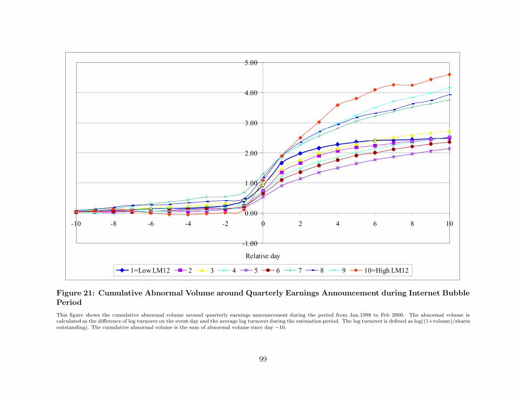
-1.00

0.00

1.00

2.00

3.00

4.00

5.00

-10 -8 -6 -4 -2 0 2 4 6 8 10

Relative day

1=Low LM12 2 3 4 5 6 7 8 9 10=High LM12

Figure 21: Cumulative Abnormal Volume around Quarterly Earnings Announcement during Internet BubblePeriod

This figure shows the cumulative abnormal volume around quarterly earnings announcement during the period from Jan.1998 to Feb 2000. The abnormal volume iscalculated as the difference of log turnover on the event day and the average log turnover during the estimation period. The log turnover is defined as log((1+volume)/sharesoutstanding). The cumulative abnormal volume is the sum of abnormal volume since day −10.

99

-1.00

0.00

1.00

2.00

3.00

4.00

5.00

-10 -8 -6 -4 -2 0 2 4 6 8 10

Relative day

1=Low LM12 2 3 4 5 6 7 8 9 10=High LM12

Figure 22: Cumulative Abnormal Volume around Quarterly Earnings Announcement during Non-BubblePeriod

This figure shows the cumulative abnormal volume around quarterly earnings announcement. Sample includes quarterly announcements of firms listed onNYSE/AMEX/NASDAQ from 1982 to 2004, excluding the period from Jan.1998 to Feb 2000. The abnormal volume is calculated as the difference of log turnoveron the event day and the average log turnover during the estimation period. The log turnover is defined as log((1+volume)/shares outstanding). The cumulative abnormalvolume is the sum of abnormal volume since day −10.

100

more difficult for liquid stocks than for illiquid stocks, we think that the results still show

pronounced speculative trading for low-LM12 stocks. During the non-bubble period, we

observe that trading volume decreases with the increase of LM12 prior to the announce-

ments. The magnitude is stronger during the non-bubble period than during the full sample

period. Therefore, the speculative trading is affected by the sentiment toward individual

stocks as well as by the market-wide sentiment. When the market-wide sentiment is high,

even illiquid stocks still have speculative trading. Therefore, during the high-sentiment

period, the differences of speculative trading between high-LM12 and low-LM12 stocks are

not as high as the differences during the low-sentiment period. These results suggest that

investor sentiment does affect trading volume.

5.5 Liquidity Premium Realized during Quarterly Earnings An-

nouncement Periods

Liu (2006) documents a liquidity premium, return of high-LM12 stocks minus return of

low-LM12 stocks, of 0.682% per month for NYSE/AMEX stocks and 0.906% for NASDAQ

stocks over a 12-month holding periods. In section 5.1, we find high-LM12 stocks earn

significantly higher abnormal returns than low-LM12 stocks around quarterly earnings

announcements. This implies that there may be a significant proportion of the annual

liquidity premium realized during the earnings announcement periods. In this section, we

calculate how much annual liquidity premium is realized during the 3-day event window

right after quarterly earnings announcements. Table 12 shows the results. We find the

average annual return is 8.13% for low-LM12 stocks and 20.27% for high-LM12 stocks.

Thus, the annual liquidity premium in our sample is 12.15%.

101

Table 12: Liquidity Premium Realized during Quarterly Earnings Announcement Periods

This table shows the returns realized during quarterly earnings announcementperiods from 1983 to 2004. In each year from July year t to June year t+1, the annual raw return

of firm i is calculated as∏jun,yr t+1

mon=jul,yr t(1+Ri,mon)−1. The market-adjusted annual return of firm i is defined as

∏jun,yr t+1

mon=jul,yr t(1+Ri,mon)−

∏jun,yr t+1

mon=jul,yr t(1+Rm,mon).

For each announcement, the raw return and market adjusted return during the event period is defined as∏2

d=0(1 + Ri,d) − 1 and

∏2

d=0(1 + Ri,d) −

∏2

d=0(1 + Rm,d) ,

respectively. For each stock, the average of all four quarterly announcements during the year from July year t to June year t + 1 is calculated first. If a stock has missingannouncements, the return of the missing announcement is replaced with the average returns of all other quarterly announcements during the same year. In each year, thecross-sectional mean of each LM12 group is calculated first. Then the time-series average of each LM12 group during the sample period is obtained. Non-event day returnis the difference between annual return and event-day return. Each year, the difference of return between low-LM12 group and high-LM12 group is taken and T-statisticsis used to test the null hypothesis that the differences are not different from zero. ***, **, and * indicate that a number is significant different from zero at 1%, 5%, and10%, respectively, from a two-tailed T test.

Raw Return Market-Adjusted ReturnAverage # Annual Event day Average # Annual Event dayLM12 Group

firms per year return (0, 2)Non-event day

firms per year return (0, 2)Non-event day

1 = low LM12 360 8.13% -0.94% 9.07% 360 -4.39% -1.52% -2.87%2 368 11.83% 0.43% 11.41% 368 -0.68% -0.22% -0.45%

3 369 14.30% 0.69% 13.61% 369 1.78% 0.11% 1.67%4 371 15.13% 1.00% 14.12% 371 2.61% 0.50% 2.11%

5 349 14.15% 0.95% 13.19% 349 1.63% 0.34% 1.30%6 313 15.80% 0.91% 14.89% 313 3.29% 0.23% 3.06%

7 287 18.18% 1.37% 16.81% 287 5.67% 0.70% 4.97%8 257 18.19% 2.28% 15.91% 257 5.67% 1.55% 4.12%

9 224 19.51% 3.35% 16.16% 224 7.00% 2.68% 4.31%10 = high LM12 153 20.27% 4.59% 15.68% 153 7.76% 4.06% 3.70%

10-1 12.15%∗∗ 5.54%∗∗∗ 6.61% 12.15%∗∗ 5.58%∗∗∗ 6.57%

102

Before we compare the liquidity premium in our sample with Liu’s (2006), we discuss

the differences between our sample and Liu’s sample. First, Liu separates NYSE/AMEX

from NASDAQ; while we mix all stocks from NYSE, AMEX, and NASDAQ together. Be-

cause the return variation for NASDAQ stocks is higher than that for NYSE/AMEX stocks,

even though we combine all stocks together, we expect the liquidity premium in our sam-

ple is more close to Liu’s NASDAQ sample than NYSE/AMEX sample. Second, because

our sample comes from the intersection of CRSP and I/B/E/S, it also reflects analysts’

preference. If analysts tend to follow firms which perform well and drop their coverage of

poor-performed firms, the returns we find would be biased toward well-performed firms.

Despite the above differences between our sample and Liu’s sample, we still find a

similar magnitude of the liquidity premium to Liu’s NASDAQ sample. In Table A.2 of

Liu (2006), the lowest-LM12 decile earn 0.559% per month. If we compound the monthly

return to generate an annual return, the lowest-LM12 stocks earn 6.92% per year. For the

highest-LM12 decile, the return is 1.466% per month, which is equivalent to 19.08% per

year. As a result, the annual liquidity premium of Liu’s NASDAQ sample is 12.16%, which

is very close to our estimate of 12.15%.

In Table 12, we find that about 5.54% raw liquidity premium and 5.58% market-

adjusted liquidity premium realized during only 12 days right after earnings announcements

(3-day period from day 0 to day 2 for four quarterly earnings announcements). Both of

the raw and market-adjusted liquidity premium realized during the quarterly earnings

announcement periods are significant at 1% level. During the non-event periods, the raw

liquidity premium is 6.61% and the market-adjusted liquid premium is 6.57%. Although

103

their magnitude is not trivial, liquidity premiums realized during non-event periods are not

significant because their time-series variation is high.

To investigate whether the liquidity premium realized during earnings announcement

periods distributes evenly over four quarters, we further classify each announcement into

one of the four quarters and redo the analysis. Table 13 provides the results. The liquidity

premium is 4.22% during the first calendar quarter, 2.11% during the second calendar

quarter, 6.29% during the third calendar quarter, and −5.07% during the fourth calendar

quarter. The Internet bubble affects the liquidity premium more significantly in the fourth

quarter than in other quarters. When we exclude the period from Jan. 1998 to Jun. 2000,

the liquidity premiums from the first calendar quarter to the fourth calendar quarter become

6.17%, 1.99%, 6.27%, and −1.88%, respectively. The variation of the liquidity premiums in

different quarters may result from the differences of seasonality between liquid and illiquid

firms. Another possible reason is that the market-wide investors sentiment may change

systematically during different quarters. For example, if in the fourth calendar quarter

investors sentiment tend to be higher than any other quarters, during this period liquid

stocks may be highly overvalued, which results in a negative liquidity premium.

Examining the 3-day abnormal return during quarterly earnings announcements, we

find that announcements made during the first and third calendar quarters exhibit higher

differences of abnormal returns between liquid and illiquid stocks than announcements in

the second and fourth calendar quarters. Because the fiscal year of most firms ends in

December, in our sample about 68% of quarterly announcements made from Jan. to Mar.

are combined with annual reports. The differences of degree of speculative trading between

104

Table 13: Liquidity Premium Realized during Quarterly Earnings Announce-ment Periods in Different QuartersThis table shows the return realized during quarterly earnings announcement periods from 1983 to 2004 in different quarters.Panel A, B, C, and D provide realized return for announcements from Jul. to Sep., from Oct. to Dec., from Jan. toMar., and from Apr. to Jun., respectively. For each announcement, the raw return and market adjusted return during the

event period is defined as∏2

d=0(1 + Ri,d) − 1 and

∏2

d=0(1 + Ri,d) −

∏2

d=0(1 + Rm,d) , respectively. In each quarter, the

cross-sectional mean of each LM12 group is calculated first. Then the time-series average of each LM12 group is obtained.Each year, the difference of return between low-LM12 group and high-LM12 group is taken and T-statistics is used to testthe null hypothesis that the differences are not different from zero. ***, **, and * indicate that a number is significantdifferent from zero at 1%, 5%, and 10%, respectively, from a two-tailed T test.

Panel A: Announcement from Jul. to Sep.Announcement from Jul. to Sep.

Raw Return Market-adjusted ReturnLM12Average #OBS

Quarterly Return 3-day (0, 2) Quarterly Return 3-day (0, 2)1=low LM12 370.95 -3.99% -0.66% -3.46% -0.68%

2 374.86 -2.28% -0.33% -1.75% -0.33%3 374.86 -1.64% -0.17% -1.12% -0.13%

4 372.45 -0.66% 0.00% -0.14% 0.05%5 350.14 -0.41% 0.12% 0.11% 0.17%

6 313.36 0.40% -0.09% 0.93% -0.06%7 282.18 -0.31% 0.02% 0.21% 0.03%

8 252.41 0.90% 0.03% 1.42% -0.01%9 217.77 3.00% 0.70% 3.53% 0.73%

10 = high LM12 142.41 2.31% 1.12% 2.83% 1.19%10-1 6.29%∗∗ 1.78%∗∗∗ 6.29%∗∗ 1.87%∗∗∗

Panel B: Announcement from Oct. to Dec.

Announcement from Oct. to Dec.Raw Return Market-adjusted ReturnLM12 Average #OBS

Quarterly Return 3-day (0, 2) Quarterly Return 3-day (0, 2)

1=low LM12 366.73 5.98% -0.12% 0.91% -0.25%2 371.95 4.64% 0.21% -0.43% -0.01%

3 373.32 4.84% 0.22% -0.23% 0.02%4 369.55 5.14% 0.15% 0.07% 0.03%

5 346.27 4.09% 0.21% -0.98% 0.02%6 310.36 2.60% 0.22% -2.47% 0.01%

7 282.09 2.71% 0.44% -2.37% 0.17%8 249.41 2.29% 0.72% -2.78% 0.50%

9 215.82 1.76% 0.36% -3.31% 0.16%10 = high LM12 138.27 0.91% 0.60% -4.16% 0.34%

10-1 -5.07% 0.72% -5.07% 0.59%

105

Table 13 continued

Panel C: Announcement from Jan. to Mar.Announcement from Jan. to Mar.

Raw Return Market-adjusted ReturnLM12 Average #OBSQuarterly Return 3-day (0, 2) Quarterly Return 3-day (0, 2)

1=low LM12 352.95 7.47% -0.19% 3.06% -0.41%

2 356.76 7.72% 0.00% 3.31% -0.18%3 362.38 7.19% 0.32% 2.78% 0.11%

4 361.67 7.67% 0.42% 3.26% 0.21%5 337.71 7.71% 0.32% 3.29% 0.11%

6 296.95 9.05% 0.40% 4.64% 0.20%7 264.67 10.84% 0.46% 6.43% 0.27%

8 228.95 11.66% 0.74% 7.25% 0.54%9 195 12.13% 1.06% 7.72% 0.85%

10 = high LM12 124.29 11.70% 1.35% 7.29% 1.14%10-1 4.22% 1.54%∗∗∗ 4.22% 1.56%∗∗∗

Panel D: Announcement from Apr. to Jun.

Announcement from Apr. to Jun.Raw Return Market-adjusted ReturnLM12 Average #OBS

Quarterly Return 3-day (0, 2) Quarterly Return 3-day (0, 2)1=low LM12 362.14 2.87% 0.05% -1.00% -0.16%

2 367.9 4.77% 0.44% 0.90% 0.21%

3 367.24 5.21% 0.31% 1.34% 0.11%4 367.29 4.87% 0.47% 1.00% 0.24%

5 343.29 4.38% 0.45% 0.51% 0.19%6 308.14 5.24% 0.46% 1.36% 0.18%

7 276.81 5.29% 0.61% 1.41% 0.36%8 249.43 5.46% 0.67% 1.59% 0.43%

9 208.14 5.05% 1.01% 1.18% 0.77%10 = high LM12 133.86 4.98% 1.24% 1.11% 0.98%

10-1 2.11% 1.19%∗∗∗ 2.11% 1.14%∗∗∗

annual announcements and quarterly announcements may be the reason for higher liq-

uidity premium for announcements in the first calendar quarters. Because there is more

information released from analysts and media before annual announcements, investors may

disagree about the precision of the available information. In Scheinkman and Xiong’s

(2003) framework, the speculative component of stock prices is higher when information

available enlarges the differences in beliefs. If we think that the liquidity premium around

quarterly earnings announcements reflects investors’ adjustments of their mispricing after

106

the announcements, the higher liquidity premium of announcements in the first calendar

quarter support Scheinkman and Xiong (2003). However, the reason for higher liquidity

premium for announcements in the third calendar quarter is not clear. Prior studies which

are related to cross-quarter differences of earnings announcements usually compare the

fourth fiscal quarter (annual announcement) with all of the interim quarters. It is not clear

why the third calendar quarter is different from the second and fourth calendar quarters. A

possible reason is the sales seasonality which results in different earnings quality in different

interim quarters.

To sum up, if we focus on the 3-day event period from day 0 to day 2, the liquidity

premium realized during the 12 days around quarterly earnings announcements is 5.54%.

It is about 45.6% of the annual liquidity premium. It is unlikely that investors require

5.54% over 12 days just to compensate liquidity risk. We believe that the 5.54% also

reflect investors’ adjustment of mispricing. Because there is more speculative trading for

low-LM12 stocks, the prices of low-LM12 stocks contain a higher speculative component

than the prices of high-LM12 stocks. After quarterly earnings announcements, investors

of low-LM12 stocks revise their overconfidence to some degree and thus the mispricing is

partially corrected, which leads to a lower announcement returns for low-LM12 stocks than

for high-LM12 stocks.

5.6 Multivariate Regression

The event study in previous sections provides univariate or bivariate tests. It cannot

control many variables at the same time. Because the earnings announcements contain

information about a firm’s fundamental value, even though the risk of the firm does not

107

change during the short event window, the liquidity premium realized during this period

may be affected by both of the information innovation and the adjustment of mispricing.

Therefore, in this section, we construct a Fama-Macbeth (1973) type regression which

controls possible factors that may affect abnormal returns around the announcements. If

the difference of abnormal returns between high-LM12 and low-LM12 firms reflect investors’

correction of their mispricing, we should observe a significant positive coefficient for LM12.

For each quarterly earnings announcement made between July year t to June year

t + 1, we calculate the following variables:

LM12 - LM12 at the end of June in year t (estimated from July year t− 1 to June year t).

Size - Log Market value (shares outstanding times price, in millions) at the end of June at

year t.

B/M - Log book-to-market ratio. Book value is obtained from the annual report in year

t − 1. Market value is estimated at the end of December in year t− 1.

Error - Analyst forecast error which equals actual earnings per share minus the consensus

of analysts’ forecast right before the announcement deflated by the stock price at the end

of June in year t.

∆Growth - Difference between the mean analysts’ estimate of long-term growth right be-

fore and right after the quarterly earnings announcement.

#Analyst - Number of analysts following right before the announcement.

Dispersion - Standard deviation of analysts’ earnings forecasts right before the announce-

ment.

LiqUp - Dummy variable which equals to 1 if a firm moves from a higher LM12 decile to

108

a lower LM12 decile from June year t to June year t + 1.

LiqDown - Dummy variable which equals to 1 if a firm moves from a lower LM12 decile to

a higher LM12 decile from June year t to June year t + 1.

∆σ - Changes of return volatility from the period (-40, -11) to period (11,40).

∆βMKTRF - Changes of systematic risk from the period (-40, -11) to period (11,40).

∆βSMB - Changes of sensitivity to SMB from the period (-40, -11) to period (11,40).

∆βHML - Changes of sensitivity to HML from the period (-40, -11) to period (11,40).

In Table 14, we provide the summary statistics of the explanatory variables used in

the regression. The I/B/E/S actuals database which provides the earnings announcement

dates has a larger coverage than the I/B/E/S summary database which provides analysts’

forecasts. Although our sample from the intersection of I/B/E/S and CRSP, on average,

contains 2768 announcements per quarter, 46.67% of observations do not have forecast

dispersions, 31.30% do not have analysts’ earnings forecasts, and 40.74% do not have

analysts’ growth forecasts. Regression analysis requires no missing value for all independent

variables. If we delete all observations which contain any missing value, on average, we lose

about 49% of observations per quarter.

As La Porta (1996) argues, the coverage of I/B/E/S summary files is heavily biased.

From panel A of Table 14, we find the sample firms without any missing value in I/B/E/S

tend to be large, liquid, growth firms with much more analysts following, higher forecast

accuracy, lower forecast dispersions, and larger downward growth revises. On the contrary,

stocks in the sample that contains missing value in I/B/E/S are small, illiquid, value stocks.

The average LM12 of these stocks is 21.43. This means, on average, these stocks do not

109

Table 14: Summary Statistics of Regression Variables

This table provides summary statistics of regression variables. Panel A shows the average of quarterly means of each variable for 82 quarters from Jul. 1984 to Dec. 2004for samples which excludes and includes OBS with missing values in I/B/E/S. Panel B shows the time-series average of cross-sectional correlation coefficients for thesample which includes OBS with missing values in I/B/E/S. For each announcement during the period from July year t to June year t + 1, the following variables arecalculated: LM12 (LM12 estimated from July year t − 1 to June year t), size (log market value (in millions) at the end of June at year t), B/M (log book-to-market ratio;book value from the annual report in year t − 1 over market value at the end of Dec year t − 1), Error (analysts?forecast error over price in June year t, in percentage),∆Growth (difference in percentage between the analysts?long-term growth forecasts right before and after the announcement, in percentage), # Analyst (number ofanalyst following), Dispersion (standard deviation of analysts?earnings forecast), LiqUp (dummy variable which equals to 1 if liquidity is upgrade from June year t to Juneyear t + 1), LiqDown (dummy variable which equals to 1 if liquidity is downgrade from June year t to June year t + 1), ∆βMKTRF (changes of systematic risk from (-40,-11) to (11,40)), ∆βSMB (changes of sensitivity to SMB from (-40, -11) to (11,40)), ∆βHML (changes of sensitivity to HML from (-40, -11) to (11,40)), )), ∆σ (changesof return volatility from (-40, -11) to (11,40), in percentage), NoEr (dummy which equals to 1 when analysts?forecast error is not found from I/B/E/S), NoGth (dummywhich equals to 1 when long-term growth is not found from I/B/E/S), and Nodps (dummy which equals to 1 when forecast dispersion is not found from I/B/E/S).

Panel A: Mean statistics for different sampleSample excludes all Sample with missing Sample includes all

missing OBS in I/B/E/S OBS in I/B/E/S missing OBS in I/B/E/S

Average OBS each quarter 1399.51 1368.57 2768.09LM12 1.6422 21.4289 11.4905Size 6.4265 4.1773 5.3057

B/M -0.7364 -0.3701 -0.5527Error -0.3947 -0.8458 -0.6126

# Analyst 6.6222 1.3215 3.5719Dispersion 0.0409 0.0918 0.0239

LiqUp 0.2251 0.2305 0.2275LiqDown 0.2679 0.3182 0.2942

∆βMKTRF -0.0107 -0.0111 -0.011∆βSMB 0.002 -0.0008 0.0019

∆βHML -0.0195 -0.0098 -0.0053∆Growth -0.1088 -0.054 -0.0602

∆σ -0.0674 0.0082 -0.0304NoEr 0 0.6126 0.313

NoDps 0 0.9307 0.4667NoGth 0 0.8105 0.4074

110

Table 14 continued

Panel B: Correlation Matrix# Disper- Liq- Liq-

LM12 Size B/M Error ∆GrowthAnalyst sion Up Down

∆βMKTRF ∆βSMB ∆βHML ∆σ NoGth NoEr NoDps

LM12 1Size -0.437 1B/M 0.233 -0.278 1

Error 0.012 0.024 -0.027 1∆Growth 0.011 -0.004 0.022 0.007 1

# Analyst -0.284 0.728 -0.232 0.008 -0.016 1Dispersion -0.070 0.105 0.017 -0.159 -0.009 0.120 1

LiqUp 0.001 -0.024 -0.014 0.009 0.009 -0.050 0.000 1LiqDown -0.123 -0.092 0.030 -0.008 -0.004 -0.079 -0.016 -0.345 1

∆βMKTRF 0.000 -0.001 0.002 -0.002 -0.002 0.000 0.002 0.006 -0.008 1∆βSMB -0.001 -0.002 0.002 -0.003 -0.001 0.000 0.002 0.005 -0.007 0.530 1

∆βSMB -0.002 0.000 -0.002 0.002 -0.003 -0.002 -0.002 0.001 -0.004 0.579 0.342 1∆σ 0.009 -0.018 0.010 -0.016 0.006 -0.014 -0.004 -0.005 0.001 0.124 0.093 0.015 1

NoGth 0.368 -0.551 0.190 0.004 0.028 -0.574 -0.129 0.001 0.048 0.001 0.001 0.001 0.019 1NoEr 0.387 -0.481 0.200 0.032 0.022 -0.515 -0.131 -0.023 0.036 0.001 0.000 0.001 0.020 0.799 1

NoDps 0.370 -0.590 0.226 -0.003 0.026 -0.656 -0.186 -0.002 0.061 0.000 -0.001 0.001 0.018 0.748 0.708 1

111

have trades for one month per year. If we delete the observations which have missing value

of analysts’ earnings forecasts, growth forecasts, and forecast dispersions, our result will be

biased toward large, liquid firms. Furthermore, because the average LM12 is 1.64 for the

sample without any missing value in I/B/E/S, these stocks are quite liquid. As a result,

the degree of mispricing among these stocks may be similar, which may lead to insignificant

regression results. To avoid losing too many observations at one time and to increase the

variation of LM12, we run stepwise regressions which include one of the forecast errors,

forecast dispersions, and changes of growth forecasts at one time. We also construct a

full-sample regression which sets the missing values of forecast errors, growth revisions,

and forecast dispersions zero and includes three dummy variables, NoEr, NoGth, and

Nodps, for the missing value in forecast errors, growth revisions, and forecast dispersions,

respectively.

Panel B of Table 14 reports the averages of the quarter by quarter cross-sectional

correlations of variables we use in regressions. The correlations are the highest between Size

and #Analyst, NoGth and NoEr, NoEr and NoDps, NoGth and NoDps, ∆βMKTRF and

∆βSMB, and between ∆βMKTRF and ∆βSMB. All other variables are not highly correlated

with each other.

For each quarter, we run a cross-sectional regression. The full-sample regression model

is as follows:

CARi = β0 + β1LM12i + β2Sizei + β3B/Mi + β4Errori + β5∆Growthi + β6#Analysti

+β7Dispersioni + β8LiqUpi + β9LiqDowni + β10∆σi + β11∆βMKTRF,i

+β12∆βSMB,i + β13∆βHML,i + β14NoGthi + β15NoEri + β16NoDpsi + ei (8)

112

In each quarter, we obtain an estimate of the coefficient for each variable and then compute

the average estimate over our sample period. We calculate the average estimate based on

two different methods. The first method is proposed by Fama and Macbeth (1973). The

average estimate of a coefficient is the equal-weighted time-series average of all quarterly

estimates. The T-statistics equals the time-series average over the standard error of the

quarterly estimates. The second method is proposed by Litzenberger and Ramaswamy

(1979). According to Litzenberger and Ramaswamy (1979), we give a different weight to

each quarterly estimate when we calculate the average across all quarters. The weight is

inversely proportional to the variance of the quarterly estimates. That is, we obtain the

weighted average estimate, weighted variance, the weight, and the T-statistics according

to the following equations:

β̂k =T∑

t=1

Zktβ̂kt, (9)

var(β̂k) =T∑

t=1

Z2ktvar(β̂kt), (10)

Zkt =

(

var(β̂kt))

−1

∑Tt=1

(

var(β̂kt))

−1 , (11)

Tk =β̂k

√

var(β̂k). (12)

Easley, Hvidkjaer, and O’Hara (2002) argue that this method weights the coefficients by

their precisions when summing across the cross-sectional regressions. Therefore, this cor-

rection technique is more efficient under time-varying volatility.

In Table 15, we show the regressions results. Panel A provides the average coefficients

when the dependent variable is the cumulative abnormal return from the Fama-French

3-factor model during the period (0, 2). In Model (1), we do not include analysts’ forecast

113

Table 15: Multivariate Regression

This table provides the results of multivariate regressions. In panel A the dependent variable is the cumulative abnormal return from Fama-French 3-factor model fromday 0 to day 2. In panel B the dependent variable is the cumulative market-adjusted return from day 0 to day 2. The dependent variable is expressed in percentage. Foreach announcement during the period from July year t to June year t + 1, the following independent variables are calculated: LM12 (LM12 estimated from July yeart − 1 to June year t), size (log market value (in millions) at the end of June at year t), B/M (log book-to-market ratio: book value from the annual report in year t − 1over market value at the end of Dec. year t − 1), Error (analysts?forecast error over price in June year t, in percentage), ∆Growth (difference in percentage betweenthe analysts?growth forecasts right before and after the announcement, in percentage), # Analyst (number of analyst following), Dispersion (standard deviation ofanalysts?earnings forecasts), LiqUp (dummy variable which equals to 1 if liquidity is upgrade from June year t to June year t + 1), LiqDown (dummy variable which equalsto 1 if liquidity is downgrade from June, year t to June year t + 1), ∆βMKTRF (changes of systematic risk from (-40, -11) to (11,40)), ∆βSMB (changes of sensitivityto SMB from (-40, -11) to (11,40)), ∆βHML (changes of sensitivity to HML from (-40, -11) to (11,40)), ∆σ (changes of return volatility from (-40, -11) to (11,40), inpercentage), NoEr (dummy which equals to 1 when analysts?forecast error is not available from I/B/E/S), NoGth (dummy which equals to 1 when long-term growth isnot available from I/B/E/S), and Nodps (dummy which equals to 1 when forecast dispersion is not available from I/B/E/S). All results are estimated from Fama andMacbeth (1973) type regressions. In each regression model, two types of the estimates are calculated. The first estimates are calculated according to Fama and Macbeth(1973). The estimates are time-series averages of coefficients from all quarterly cross-sectional regressions. T-statistics (in parenthesis) is calculated from the ratio of themean coefficient over 82 quarters to the standard errors of the 82 coefficients. The second estimates are computed according to Litzenberger and Ramaswamy (1979). Theestimates are weighted means of the quarterly estimates, where the weights are inversely proportional to the variances of these estimates. In model (2), (3), (4), and (5),the third calendar quarter in 1984 is removed because it only has 12 non-missing observations when we exclude missing forecast error, forecast dispersion, and growth forecast.

114

Table 15 continued

Panel A: Regression of cumulative abnormal return from Fama and French 3-factor Model from day 0 to day 2(1) (2) (3) (4) (5) (6)

ModelF-M L-R F-M L-R F-M L-R F-M L-R F-M L-R F-M L-R

Avg # OBS 2768 2768 1954 1954 1655 1655 1527 1527 1416 1416 2768 27680.4130 0.3533 0.0141 -0.0051 -0.0099 -0.0073 -0.0933 -0.0847 0.1074 0.0775 0.6135 0.5912

Intercept(3.40) (4.50) (0.09) (-0.06) (-0.06) (-0.07) (-0.56) (-0.80) (0.62) (0.71) (4.64) (6.48)0.0084 0.0094 0.0071 0.0062 0.0095 0.0066 0.0101 0.0105 0.0074 0.0099 0.0081 0.0091

LM12(6.70) (12.97) (3.27) (4.64) (2.94) (3.83) (2.80) (4.22) (1.53) (3.58) (6.51) (12.09)-0.0606 -0.0531 0.027 0.0296 0.0387 0.0377 0.0565 0.0524 0.0275 0.0282 -0.0789 -0.0730

Size(-3.00) (-3.49) (1.17) (1.69) (1.60) (2.06) (2.31) (2.75) (1.08) (1.45) (-3.90) (-4.71)0.2107 0.2255 0.1684 0.1872 0.1637 0.1612 0.1946 0.1855 0.1636 0.1557 0.2153 0.2267

B/M(5.89) (9.89) (3.89) (7.36) (4.38) (5.90) (5.19) (6.60) (4.17) (5.33) (6.23) (9.89)

0.0468 0.0019 0.2154 0.0052 0.0502 0.0020Error

(4.33) (6.35) (4.57) (4.20) (4.00) (4.89)0.0346 0.0344 0.0084 0.0071 0.0023 0.0006 0.0015 -0.0009 0.0027 0.0002 0.0316 0.0308

# Analyst(5.9) (6.22) (1.37) (1.22) (0.37) (0.10) (0.23) (-0.15) (0.41) (0.04) (4.49) (5.09)

-0.9446 -0.0261 -0.5807 -0.1205 -0.467 -0.021Dispersion

(-3.29) (-1.41) (-1.45) (-2.63) (-1.29) (-0.82)0.2017 0.1937 0.1684 0.1444 0.1207 0.0910 0.1450 0.139 0.1038 0.0909 0.1979 0.1915

LiqUp(3.01) (4.32) (2.58) (3.03) (1.94) (1.81) (2.21) (2.66) (1.57) (1.70) (2.96) (4.27)-0.1077 -0.1069 -0.0849 -0.0785 -0.0605 -0.0463 -0.0919 -0.0739 -0.0586 -0.0424 -0.1014 -0.1015

LiqDown(-2.07) (-2.51) (-1.41) (-1.71) (-1.14) (-0.96) (-1.64) (-1.47) (-1.04) (-0.83) (-1.94) (-2.38)0.1292 0.1407 0.1426 0.1661 0.1432 0.1602 0.1575 0.2035 0.1696 0.1987 0.1313 0.1416

∆βMKTRF (3.00) (12.16) (2.67) (11.19) (2.38) (9.53) (2.42) (11.38) (2.60) (10.51) (3.06) (12.24)-0.0162 -0.0093 -0.0195 -0.0162 -0.0252 -0.0242 -0.0317 -0.0316 -0.0472 -0.0476 -0.0167 -0.0082

∆βSMB (-0.51) (-1.25) (-0.53) (-1.67) (-0.66) (-2.21) (-0.86) (-2.69) (-1.29) (-3.85) (-0.53) (-1.10)-0.0113 -0.0241 -0.0078 -0.0188 -0.0107 -0.0181 -0.0206 -0.0289 -0.0185 -0.0315 -0.0126 -0.0262

∆βHML (-0.40) (-4.26) (-0.28) (-2.57) (-0.32) (-2.20) (-0.60) (-3.30) (-0.53) (-3.41) (-0.45) (-4.62)0.1139 0.0891 0.1366 0.1113 0.0849 0.0915

∆Growth(7.63) (10.23) (8.09) (11.2) (2.71) (9.18)

-0.2272 -0.2316 -0.2477 -0.2565 -0.3052 -0.3047 -0.2841 -0.3029 -0.2818 -0.3026 -0.2230 -0.2275∆σ

(-7.98) (-23.87) (-7.21) (-18.44) (-7.80) (-18.92) (-7.358) (-17.58) (-6.90) (-16.52) (-7.76) (-23.42)0.146 0.2483

NoEr(1.48) (3.69)0.1020 -0.0842

NoDps(-1.52) (-1.38)-0.1386 -0.2800

NoGth(-1.08) (-4.20)

R̄2 0.0241 0.0279 0.0244 0.0232 0.0326 0.0278

115

Table 15 continued

Panel B: Regression of cumulative market-adjusted return from day 0 to day 2(1) (2) (3) (4) (5) (6)

ModelF-M L-R F-M L-R F-M L-R F-M L-R F-M L-R F-M L-R

Avg # OBS 2768 2768 1954 1954 1655 1655 1527 1527 1416 1416 2768 27680.3508 0.2762 -0.0117 -0.0362 -0.0068 -0.0255 -0.1003 -0.0907 0.1239 0.0732 0.549 0.5222

Intercept(2.72) (3.69) (-0.06) (-0.41) (-0.03) (-0.26) (-0.46) (-0.89) (0.55) (0.69) (3.63) (6.01)0.0073 0.0082 0.0058 0.0054 0.0076 0.0053 0.0086 0.0073 0.0057 0.0065 0.0072 0.0080

LM12(6.06) (11.88) (2.81) (4.17) (2.56) (3.20) (2.28) (3.08) (1.43) (2.45) (6.07) (11.19)-0.0553 -0.0435 0.0279 0.0313 0.0346 0.0359 0.0551 0.0518 0.0223 0.0266 -0.0734 -0.0631

Size(-2.59) (-3.00) (0.95) (1.86) (1.07) (2.03) (1.61) (2.82) (0.63) (1.42) (-3.35) (-4.28)0.2223 0.2417 0.1879 0.2077 0.1690 0.1777 0.2045 0.2071 0.1656 0.1706 0.2234 0.2406

B/M(5.64) (11.11) (4.35) (8.49) (4.22) (6.74) (4.71) (7.62) (3.78) (6.04) (5.76) (10.99)

0.0406 0.0014 0.2128 0.0048 0.0438 0.0018Error

(3.87) (5.16) (4.47) (3.90) (3.59) (4.52)0.0393 0.0356 0.0138 0.0089 0.0078 0.0030 0.0064 0.0007 0.0078 0.0015 0.0368 0.0309

# Analyst(6.34) (6.74) (1.94) (1.59) (1.05) (0.54) (0.81) (0.12) (0.99) (0.25) (5.20) (5.34)

-0.7941 -0.0298 -0.3524 -0.0910 -0.3076 -0.0206Dispersion

(-2.59) (-1.67) (-0.86) (-2.10) (-0.86) (-0.84)0.2146 0.2029 0.1710 0.1491 0.1286 0.1068 0.1209 0.1206 0.0736 0.0755 0.2064 0.1970

LiqUp(3.10) (4.76) (2.61) (3.26) (2.04) (2.21) (1.74) (2.40) (1.06) (1.46) (3.00) (4.62)-0.1008 -0.1139 -0.1034 -0.1003 -0.0894 -0.0714 -0.1271 -0.0999 -0.1028 -0.0739 -0.0976 -0.1102

LiqDown(-1.96) (-2.81) (-1.74) (-2.28) (-1.74) (-1.54) (-2.32) (-2.06) (-1.80) (-1.49) (-1.92) (-2.71)0.1078 0.0743 0.1665 0.1210 0.1900 0.1309 0.2033 0.1612 0.2157 0.1625 0.1090 0.0751

∆βMKTRF (3.89) (6.75) (4.33) (8.48) (4.44) (8.06) (4.38) (9.32) (4.56) (8.89) (3.90) (6.82)0.0308 0.0235 0.0245 0.0138 0.0171 0.0106 0.0073 0.0024 -0.0051 -0.0108 0.0306 0.0249

∆βSMB (2.28) (3.29) (1.36) (1.47) (0.80) (1.01) (0.32) (0.21) (-0.23) (-0.90) (2.24) (3.49)-0.0383 -0.0172 -0.0537 -0.0232 -0.0608 -0.0318 -0.0628 -0.0321 -0.0601 -0.0363 -0.0391 -0.0190

∆βHML (-2.93) (-3.20) (-3.43) (-3.31) (-2.96) (-4.00) (-2.92) (-3.80) (-2.80) (-4.07) (-2.97) (-3.53)0.1170 0.0905 0.1408 0.1156 0.0782 0.0939

∆Growth(7.63) (10.71) (8.03) (11.94) (1.90) (9.80)

-0.2378 -0.2396 -0.2869 -0.2852 -0.3579 -0.3524 -0.3292 -0.3431 -0.3311 -0.3502 -0.2327 -0.2355∆σ

(-9.59) (-25.82) (-10.16) (-21.28) (-10.23) (-22.65) (-9.24) (-20.58) (-8.88) (-19.76) (-9.27) (-25.36)0.1856 0.2219

NoEr(2.33) (3.46)-0.0534 -0.0759

NoDps(-0.92) (-1.30)-0.2408 -0.2838

NoGth(-2.93) (-4.46)

R̄2 0.0119 0.0154 0.0141 0.0133 0.0237 0.0153

116

errors, forecast dispersions, and changes of growth forecasts. In Model (2), Model (3), and

Model (4), we add forecast errors, forecast dispersions, and changes of growth forecasts to

the regression model, respectively. Model (5) includes the three variables in the regression

but deletes announcements with any missing value in I/B/E/S. In Model (6), we report

the estimates from the regression which includes all variables and announcements.

Examining the Fama-Macbeth estimates, we find that the T-statistics of the coeffi-

cients of LM12 are larger than 2 in all models except Model (5). Because the stocks in

Model (5) are all quite liquid, and the T-statistics of the LM12 coefficient increases with

the number of observations, we conjecture that the low variation of LM12 for stocks in

Model (5) leads to the insignificant result.

Focusing on the Litzenberger-Ramaswamy weighted-average estimates, we find the

estimates in all models are significant, including Model (5). The T-statistics of these

estimates are all higher than 2. Because investor sentiment changes over time, if the

coefficient of LM12 captures the effect of speculative trading, possibly the volatility of the

estimates also changes over time. In this case, Litzenberger-Ramaswamy estimates can be

more efficient because they consider time-varying volatility.

Our results indicate that after controlling for possible factors of the returns around

quarterly earnings announcements, LM12 still have significant effects on the announcement

returns. From Model (6) which includes all announcements in our sample, we find when the

number of non-trading day increases by one day, the 3-day cumulative abnormal return in-

creases by 0.0091%. In Table 1, the difference of average LM12 between the highest-LM12

decile and the lowest-LM12 decile is 112.83 days. Therefore, after controlling for other

117

possible factors, about 1.0268% premium is realized during the 3-day quarterly earnings

announcement period and each year about 4.1070% is realized during the 12-day announce-

ment period. In panel B of Table 15, we use the cumulative market-adjusted return from

day 0 to day 2 as the dependent variable in the regressions. The results are quite similar

to those in panel A. After controlling for other factors, each year about 3.6106% premium

occurs during the 12-day quarterly earnings announcement period.

Following Brennan, Chordia, and Subrahmanyam (1998)10, we also run a regression

which expresses the explanatory variables for a given quarter as deviations from their cross-

sectional means for that quarter. The results are presented in Table 16. Because in the

regression, the coefficient of each explanatory variable captures the effect of a shock of

one standard deviation from cross-sectional mean on the abnormal return, in panel A we

first report the average of cross-sectional mean and standard deviation for each regression

model. Generally speaking, when the average number of the observations in a regression

model is larger, the cross-sectional mean and standard deviation of LM12 are larger.

Panel B of Table 16 shows the regression results when the dependent variable is the

3-day cumulative abnormal return from Fama and French 3-factor model. We find the

coefficients of LM12 in all of the 6 regression models are significant positive. In Model

(6) which includes all observations of our sample, the Litzenberger-Ramaswamy estimate

is 0.2322. This means when the LM12 increases by one standard deviation from 11.49 to

38.57, the 3-day cumulative abnormal return from day 0 to day 2 increases by 0.2322%.

10In Brennan, Chordia, and Subrahmanyam’s (1998) regression model, the dependent variable is therisk-adjusted return and the explanatory variables are non-risk firm characteristics. They argue that theregression model implies that the explanatory variables of the average security are zero and thus its expectedreturn is determined solely by its risk characteristics.

118

Table 16: Robustness Check of Multivariate Regression

This table provides the results of multivariate regressions. All explanatory variables are expressed as the deviation from cross-sectional mean ((variable?mean)/standarddeviation). We report the average of cross-sectional mean and standard deviation in Panel A. In panel B the dependent variable is the cumulative abnormal return fromFama-French 3-factor model from day 0 to day 2. In panel C the dependent variable is the cumulative market-adjusted return from day 0 to day 2. The dependent variableis expressed in percentage. For each announcement during the period from July year t to June year t + 1, the following independent variables are calculated: LM12 (LM12estimated from July year t − 1 to June year t), size (log market value (in millions) at the end of June at year t), B/M (log book-to-market ratio: book value from theannual report in year t− 1 over market value at the end of Dec. year t− 1), Error (analysts?forecast error over price in June year t, in percentage), ∆Growth (difference inpercentage between the analysts?growth forecasts right before and after the announcement, in percentage), # Analyst (number of analyst following), Dispersion (standarddeviation of analysts?earnings forecasts), LiqUp (dummy variable which equals to 1 if liquidity is upgrade from June year t to June year t + 1), LiqDown (dummy variablewhich equals to 1 if liquidity is downgrade from June, year t to June year t + 1), ∆βMKTRF (changes of systematic risk from (-40, -11) to (11,40)), ∆βSMB (changes ofsensitivity to SMB from (-40, -11) to (11,40)), ∆βHML (changes of sensitivity to HML from (-40, -11) to (11,40)), ∆σ (changes of return volatility from (-40, -11) to (11,40),in percentage), NoEr (dummy which equals to 1 when analysts?forecast error is not available from I/B/E/S), NoGth (dummy which equals to 1 when long-term growthis not available from I/B/E/S), and Nodps (dummy which equals to 1 when forecast dispersion is not available from I/B/E/S). All results are estimated from Fama andMacbeth (1973) type regressions. In each regression model, two types of the estimates are calculated. The first estimates are calculated according to Fama and Macbeth(1973). The estimates are time-series averages of coefficients from all quarterly cross-sectional regressions. T-statistics (in parenthesis) is calculated from the ratio of themean coefficient over 82 quarters to the standard errors of the 82 coefficients. The second estimates are computed according to Litzenberger and Ramaswamy (1979). Theestimates are weighted means of the quarterly estimates, where the weights are inversely proportional to the variances of these estimates. In model (2), (3), (4), and (5),the third calendar quarter in 1984 is removed because it only has 12 non-missing observations when we exclude missing forecast error, forecast dispersion, and growth forecast.

Panel A: Average cross-sectional mean and standard deviation(1) (2) (3) (4) (5) (6)

Standard Standard Standard Standard Standard StandardModelMean deviation Mean deviation Mean deviation Mean deviation Mean deviation Mean deviation

Avg # OBS 2768 2768 1954 1954 1655 1655 1527 1527 1416 1416 2768 2768LM12 11.4905 27.08 4.4093 14.23 3.0685 11.03 1.9344 7.91 1.6617 7.06 11.4905 27.08Size 5.3057 1.85 5.9018 1.69 6.1555 1.63 6.3322 1.59 6.4299 1.57 5.3057 1.85B/M -0.5527 0.82 -0.6682 0.77 -0.6903 0.75 -0.7322 0.76 -0.7341 0.75 -0.5527 0.82Error -0.8834 32.28 -0.3688 10.93 -0.6111 26.73# Analyst 3.5719 4.57 5.1687 4.75 5.7966 4.87 6.3842 4.75 6.6453 4.8 3.5719 4.57Dispersion 0.0446 0.49 0.0399 0.33 0.0239 0.37LiqUp 0.2275 0.42 0.2339 0.42 0.2282 0.41 0.2288 0.41 0.2248 0.41 0.2275 0.42LiqDown 0.2942 0.45 0.2856 0.44 0.2801 0.43 0.2711 0.43 0.2702 0.42 0.2942 0.45∆βMKTRF -0.011 2.33 -0.0125 1.95 -0.0129 1.82 -0.0129 1.77 -0.012 1.72 -0.011 2.33∆βSMB 0.0019 3.06 0.0013 2.54 0.0001 2.37 0.0025 2.29 0.0034 2.22 0.0019 3.06∆βHML -0.0053 3.84 -0.0066 3.2 -0.0061 2.95 -0.0035 2.88 -0.0021 2.79 -0.0053 3.84∆Growth -0.1017 2.13 -0.1104 1.99 -0.0602 1.62∆σ -0.0304 1.87 -0.0544 1.42 -0.06193 1.29 -0.0654 1.25 -0.0688 1.21 -0.0304 1.87NoEr 0.3078 0.45NoDps 0.4667 0.49NoGth 0.4074 0.48

119

Table 16 continued

Panel B: Regression of cumulative abnormal return from Fama and French 3-factor Model from day 0 to day 2(1) (2) (3) (4) (5) (6)

ModelF-M L-R F-M L-R F-M L-R F-M L-R F-M L-R F-M L-R

Avg # OBS 2768 2768 1954 1954 1655 1655 1527 1527 1416 1416 2768 27680.1981 0.1728 0.1186 0.0941 0.1522 0.1273 0.1267 0.1031 0.1511 0.1239 0.1981 0.1724

Intercept(6.73) (10.02) (3.66) (5.11) (4.77) (6.63) (3.99) (5.18) (4.79) (6.12) (6.73) (10.02)0.2461 0.2409 0.1017 0.0881 0.1005 0.0758 0.0885 0.0810 0.0738 0.0652 0.2380 0.2322

LM12(7.36) (12.06) (3.74) (4.38) (3.32) (3.67) (3.85) (3.82) (2.79) (3.03) (7.14) (11.27)-0.1139 -0.0959 0.0455 0.0497 0.0634 0.0608 0.0921 0.0806 0.0437 0.0429 -0.1480 -0.1320

Size(-3.06) (-3.44) (1.16) (1.69) (1.56) (2.04) (2.33) (2.68) (1.07) (1.42) (-3.96) (-4.65)0.1883 0.1678 0.1431 0.1304 0.1290 0.1123 0.1545 0.1297 0.1275 0.1078 0.1904 0.1700

B/M(6.05) (9.11) (4.19) (6.77) (4.32) (5.60) (5.21) (6.24) (4.16) (5.07) (6.34) (9.18)

0.8040 0.2790 0.5825 0.3271 0.2326 0.2358Error

(5.70) (14.93) (4.13) (13.93) (5.30) (12.87)0.1645 0.1508 0.0451 0.0313 0.0170 0.0014 0.0077 -0.0012 0.0152 0.0005 0.1474 0.1369

# Analyst(6.01) (5.89) (1.57) (1.13) (0.56) (0.05) (0.24) (-0.04) (0.48) (0.02) (4.67) (4.83)

-0.1070 -0.1046 0.0780 -0.0788 -0.0452 -0.0452Dispersion

(-3.78) (-5.17) (0.57) (-3.34) (-1.80) (-2.41)0.0854 0.0793 0.0720 0.0590 0.0494 0.0376 0.0606 0.0555 0.0422 0.0361 0.0838 0.0785

LiqUp(3.12) (4.25) (2.70) (2.96) (2.02) (1.81) (2.32) (2.58) (1.63) (1.65) (3.08) (4.20)-0.0451 -0.0513 -0.0345 -0.0382 -0.0222 -0.0239 -0.0368 -0.0351 -0.0230 -0.0209 -0.0423 -0.0487

LiqDown(-1.94) (-2.68) (-1.32) (-1.89) (-0.97) (-1.14) (-1.54) (-1.63) (-0.97) (-0.96) (-1.82) (-2.55)0.3009 0.3295 0.2824 0.3240 0.2637 0.2891 0.2972 0.3537 0.2960 0.3401 0.3054 0.3313

∆βMKTRF (3.12) (12.10) (2.97) (11.21) (2.73) (9.53) (2.87) (11.24) (2.98) (10.59) (3.18) (12.17)-0.0515 -0.0148 -0.0369 -0.0203 -0.0713 -0.0336 -0.0803 -0.0483 -0.1134 -0.0812 -0.0524 -0.0125

∆βSMB (-0.64) (-0.63) (-0.39) (-0.82) (-0.94) (-1.29) (-1.13) (-1.78) (-1.63) (-2.94) (-0.65) (-0.53)-0.0597 -0.0808 -0.0431 -0.0460 -0.0433 -0.0404 -0.0744 -0.0618 -0.0641 -0.0674 -0.0649 -0.0879

∆βHML (-0.59) (-3.53) (-0.50) (-1.91) (-0.46) (-1.61) (-0.78) (-2.38) (-0.67) (-2.55) (-0.64) (-3.84)0.2270 0.1991 0.2595 0.2259 0.1685 0.1564

∆Growth(7.51) (10.29) (8.08) (11.03) (7.22) (9.04)

-0.4270 -0.3997 -0.3505 -0.3400 -0.3936 -0.3637 -0.3652 -0.3442 -0.3578 -0.3253 -0.4195 -0.3925∆σ

(-8.26) (-22.51) (-7.71) (-17.73) (-7.68) (-18.13) (-7.28) (-16.49) (-6.73) (-15.22) (-8.07) (-22.08)0.0797 0.1110

NoEr(1.98) (3.63)-0.0382 -0.0420

NoDps(-1.32) (-1.39)-0.1028 -0.1341

NoGth(-2.48) (-4.12)

R̄2 0.0241 0.0279 0.0244 0.0232 0.0326 0.0278

120

Table 16 continued

Panel C: Regression of cumulative market-adjusted return from day 0 to day 2(1) (2) (3) (4) (5) (6)

ModelF-M L-R F-M L-R F-M L-R F-M L-R F-M L-R F-M L-R

Avg # OBS 2768 2768 1954 1954 1654 1654 1527 1527 1417 1417 2768 27680.1837 0.1414 0.1258 0.0837 0.1637 0.1201 0.1438 0.0979 0.1695 0.1186 0.1837 0.1410

Intercept(4.40) (8.61) (2.88) (4.74) (3.66) (6.49) (3.19) (5.11) (3.72) (6.08) (4.40) (8.60)0.2162 0.2099 0.0840 0.0763 0.0782 0.0601 0.0699 0.0571 0.0519 0.0406 0.2118 0.2041

LM12(6.59) (11.04) (3.28) (3.95) (2.88) (3.02) (3.23) (2.79) (2.35) (1.96) (6.67) (10.41)-0.1043 -0.0780 0.0471 0.0526 0.0565 0.0579 0.0885 0.0801 0.0342 0.0412 -0.1382 -0.1135

Size(-2.63) (-2.94) (0.94) (1.87) (1.05) (2.01) (1.62) (2.77) (0.61) (1.41) (-3.38) (-4.20)0.2001 0.1777 0.1609 0.1421 0.1367 0.1201 0.1673 0.1401 0.1338 0.1136 0.1997 0.1780

B/M(5.66) (10.14) (4.39) (7.69) (4.01) (6.23) (4.51) (6.99) (3.64) (5.54) (5.76) (10.09)

0.2516 0.2429 0.5783 0.2961 0.2108 0.2068Error

(5.56) (13.54) (4.20) (13.08) (5.13) (11.85)0.1835 0.1584 0.0652 0.0443 0.0382 0.0179 0.0269 0.0095 0.0352 0.0118 0.1622 0.1414

# Analyst(6.33) (6.50) (1.96) (1.66) (1.07) (0.65) (0.74) (0.34) (0.95) (0.42) (5.36) (5.23)

-0.0865 -0.0898 0.1122 -0.0566 -0.0269 -0.0312Dispersion

(-2.94) (-4.60) (0.85) (-2.49) (-1.05) (-1.75)0.0908 0.0827 0.0734 0.0602 0.0536 0.0426 0.0514 0.0464 0.0309 0.0280 0.0874 0.0803

LiqUp(3.23) (4.66) (2.74) (3.15) (2.13) (2.14) (1.83) (2.24) (1.12) (1.53) (3.13) (4.51)-0.0426 -0.0540 -0.0435 -0.0472 -0.0352 -0.0342 -0.0511 -0.0463 -0.0414 -0.0338 -0.0412 -0.0523

LiqDown(-1.86) (-2.97) (-1.69) (-2.43) (-1.57) (-1.70) (-2.15) (-2.23) (-1.70) (-1.60) (-1.82) (-2.87)0.2200 0.2055 0.2826 0.2670 0.2948 0.2666 0.3136 0.3135 0.3192 0.3071 0.2228 0.2072

∆βMKTRF (3.61) (7.90) (4.10) (9.59) (4.24) (9.09) (4.31) (10.29) (4.42) (9.87) (3.62) (7.97)0.0748 0.0904 0.0372 0.0517 0.0240 0.0444 0.0065 0.0231 -0.0230 -0.0067 0.0755 0.0935

∆βSMB (1.88) (4.05) (0.90) (2.15) (0.55) (1.76) (0.15) (0.88) (-0.52) (-0.25) (1.80) (4.19)-0.1351 -0.0772 -0.1678 -0.0770 -0.1776 -0.0920 -0.1758 -0.0918 -0.1660 -0.0963 -0.1391 -0.0829

∆βHML (-2.68) (-3.55) (-3.52) (-3.33) (-3.05) (-3.81) (-3.04) (-3.66) (-2.89) (-3.78) (-2.73) (-3.81)0.2340 0.2011 0.2697 0.2316 0.1740 0.1591

∆Growth(7.39) (10.79) (7.82) (11.74) (7.07) (9.66)

-0.4497 -0.4109 -0.4111 -0.3745 -0.4739 -0.4119 -0.4331 -0.3824 -0.4303 -0.3683 -0.4414 -0.4036∆σ

(-9.48) (-24.31) (-9.71) (-20.34) (-9.72) (-21.31) (-8.86) (-18.99) (-8.39) (-17.88) (-9.22) (-23.85)0.0798 0.1007

NoEr(2.19) (3.46)-0.0309 -0.0373

NoDps(-1.10) (-1.29)-0.1163 -0.1370

NoGth(-2.90) (-4.41)

R̄2 0.0119 0.0154 0.0141 0.0133 0.0237 0.0153

121

Because the difference of LM12 between high-LM12 and low-LM12 stocks is 112.83 (about

4.17 standard deviations), for each quarterly announcement the 3-day abnormal return of

high-LM12 stocks is estimated to be higher by 0.9674% than low-LM12 stocks. Each year,

the perceived liquidity premium realized around the 12-day announcement period is about

3.8699%, which is quite close to the magnitude in Table 15.

In Model (5) of panel B, although the estimate of the LM12 coefficient are very

different from that in Model (6), because the cross-sectional standard deviation of LM12 in

Model (5) is lower, the economic effect of LM12 in Model (5) is similar to that in Model (6).

The average cross-sectional standard deviation of LM12 in Model (5) is 7.06. When the

LM12 increases by 7.06, the 3-day abnormal return increases by 0.0652%. The difference

of 112.83 between liquid and illiquid stocks is about 15.98 standard deviations. Therefore,

from Model (5), the premium realized during the 3-day announcement period is about

1.0420% per quarter or 4.1680% per year.

In panel C of Table 16, we provide the results when the dependent variable is the 3-day

market-adjusted return. The effect of LM12 on the event-day return is not as strong as

the effect in panel B. In model (6), when the LM12 increases by 27.08, the 3-day abnormal

return increases by 0.2041%. In model (5), when the LM12 increases by 7.06, the 3-day

abnormal return increases by 0.0406%. This implies that the liquidity premium realized

during the 12-day announcement period is 3.4016% in Model (6) and 2.5954% in Model

(5).

To sum up, the magnitude of the perceived liquidity premium realized during quarterly

earnings announcement periods is not trivial. If we focus on Model (6) of Table 15 and use

122

the abnormal return from Fama-French 3-factor model as the dependent variable, we find

the liquidity premiums realized during the 12-day announcement period is about 4.11%,

which is around one-third annual liquidity premium. Because it is hard to explain why there

is a non-trivial liquidity premium realized during the 12-day quarterly announcement period

after controlling for possible factors, we believe it reflects the adjustment of mispricing after

quarterly earnings announcements by overconfident investors. Our results support the

third hypothesis that the perceived liquidity premium is partially driven by the speculative

trading of overconfident investors.

123

Chapter 6 Conclusion

This study investigates whether stock price reactions to quarterly earnings announce-

ments depend on stock liquidity. Our hypotheses are derived from Baker and Stein (2004)

and Scheinkman and Xiong (2003). With differences in beliefs from overconfident investors

and short-sale constraints, the liquidity of stocks is magnified by speculative trading of opti-

mistic overconfident investors. Thus, liquid stocks tend to be more overpriced than illiquid

stocks. We hypothesize that quarterly earnings announcements convey information about

firms’ fundamental values, which triggers and synchronizes investors’ revisions of their mis-

pricing. Therefore, right after the quarterly earnings announcements, liquid stocks which

contain a larger speculative component in their prices prior to the announcements should

show a lower abnormal return than illiquid stocks.

Investigating the return and trading activities around quarterly earnings announce-

ment, we find evidences support our hypothesis. The abnormal returns right after quarterly

earnings announcements decrease with the liquidity of the stock. The differences of cumu-

lative abnormal returns between the most liquid stocks and the least liquid stocks is 1.91%

during the 3-day period from day 0 to day 2. This difference is robust after we control

for firm size, book-to-market, earnings forecast errors, revisions of growth forecasts, ana-

lyst forecasts dispersions, changes of return volatility, changes of future liquidity, and for

changes in risk.

From the abnormal trading volume and the path of cumulative abnormal returns

during the announcement period, we find evidence of speculative trading for liquid stocks

124

prior to the announcements. Before the announcement, the trading volume decreases and

the drop in volume decreases with the increase in liquidity. The cumulative abnormal

returns of liquid stocks increase significantly prior to the announcements but decrease

significantly after the announcements. Because we do not observe the same return pattern

for illiquid stocks and the volume drop prior to the announcements for liquid stocks is

lower than illiquid stocks, the result indicates that before the announcements, speculative

trading occurs more frequently for liquid stocks than for illiquid stocks. This pattern

of speculative trading holds particularly for small, growth, high-forecast-dispersion, low-

analyst-following stocks whose valuation tend to be subjective, which also supports Baker

and Wurgler (2006).

In the further analysis of the different announcement effects on liquid and illiquid

stocks, we find liquidity premium realized during the 12-day period right after quarterly

earnings announcements is 5.54%. It is about 45.6% of the perceived annual liquidity

premium. After controlling other factors in a regression, we still find about 4.11% liquidity

premium per year occurs during the quarterly earnings announcements. The magnitude is

not trivial. These results support our hypothesis that liquidity premium can be partially

explained by the speculative trading from overconfident investors. They also suggest that

earnings announcements can serve as an important mechanism for regulating overpricing

caused by speculative trading.

Our findings contribute to the debate on whether investors’ behavior affects stock

prices. The effect of investors’ speculative trading on stock prices is not negligible. Given

the excessive trading activities on the stock market and the sizable liquidity premium

125

per year, we believe there is a non-trivial component of stock prices resulted from non-

fundamental non-risk factors. Thus, for future research, incorporating investors’ sentiment

or speculative behavior into an asset pricing model and identifying the magnitude of irra-

tional investors’ influence on stock prices are promising research areas.

126

References

Abreu, D. and M.K. Brunnermeier, 2003. “Bubbles and Crashes,” Econometrica,Vol. 71, No. 1, pp. 173-204.

Acharya, V.V., and L.H. Pedersen, 2005. “Asset pricing with liquidity risk,” Journal

of Financial Economics, 77, pp. 375-410.

Admati, A., and P. Pfleiderer, 1988. “A theory of intraday patterns: Volume andprice variability,” Review of Financial Studies, 1, pp. 3-40.

Amihud, Y., 2002. “Illiquidity and stock returns,” Journal of Financial Markets, 5,pp. 31-56.

Amihud, Y. and H. Mendelson, 1986. “Asset pricing and the bid-ask spread,” Journal

of Financial Economics, 17, pp. 223-249.

Atiase, R.K., 1985. “Predisclosure information, firm capitalization, and security pricebehavior around earnings announcements ,” Journal of Accounting Research, Vol. 23,No. 1 , pp. 21-36.

Atkins, A.B., and E.A. Dyl, 1997. “Market Structure and Reported Trading Volume:NASDAQ versus the NYSE,” Journal of Financial Research, Vol. XX, No. 3, pp.291-304.

Baker, M. and J. Stein, 2004. “Market liquidity as a sentiment indicator,” Journal

of Financial Markets, 7, pp. 271-299.

Baker, M. and J. Wurgler, 2006. “Investor sentiment and the cross-section of stockreturns,” Journal of Finance, 61, pp. 1645-1680.

Black, F., 1986. “Noise,” Journal of Finance, Vol. XLI, No. 3, pp. 529-543.

Brennan, M.J., T. Chordia, and A. Subrahmanyam, 1998. “Alternative factor spec-ifications, security characteristics, and the cross-section of expected stock returns,”Journal of Financial Economics, 49, pp. 345-373.

Brennan, M.J. and A. Subrahmanyam, 1996. “Market microstructure and asset pric-ing: On the compensation for illiquidity in stock returns,” Journal of Financial Eco-

nomics, 41, pp. 441-464.

127

Brown, G.W. and M.T. Cliff, 2005. “Investor sentiment and asset valuation,” Journal

of Business, Vol. 78, No. 2, pp. 405-440.

Campbell, J.Y. and A.S. Kyle, 1993. “Smart money, noise trading and stock pricebehaviour,” Review of Economic Studies, 60, pp. 1-34.

Chae, J, 2005. “Trading Volume, Information Asymmetry, and Timing Information,”Journal of Finance, Vol. LX, No. 1, pp. 413-442.

Datar, V., N.Y. Naik, and R. Radcliffe, 1998. “Liquidity and stock returns: Analternative test,” Journal of Financial Markets, 1, pp. 203-219.

Diether, K.B., C.J. Malloy, and A. Scherbina, 2002. “Differences of opinion and thecross section of stock returns,” Journal of Finance, 57, pp. 2113-2141.

Easley, D. and M. O’Hara, 1992.“Adverse selection and large trade volume: Theimplications for market efficiency,” Journal of Financial and Quantitative Analysis,Vol. 27, pp185-208.

Easley, D., S. Hvidkjaer, and M. O’Hara, 2002.“Is information risk a determinant ofasset returns?,” Journal of Finance, Vol. 57, pp2185-2221.

Fama, E.F., and K.R. French, 1993. “Common risk factors in the returns on stocksand bonds,” Journal of Financial Economics, 33, pp. 3-56.

Fama, E.F., and J. Macbeth, 1973. “Risk, return, and equilibrium: Empirical tests,”Journal of Political Economics, 71, pp.607-636.

Frazzini, A., and O. Lamont, 2006. “The earnings announcement premium andtrading volume,” working paper, University of Chicago.

Glaser, M., and M. Weber, 2003. “Overconfidence and trading volume,” workingpaper, University Mannheim.

Hong, H., T. Lim, and J. Stein, 2000. “Bad news travels slowly: Size, analyst coverageand the profitability of momentum strategies,” Journal of Finance, 55, pp. 265-296.

Johnson, S., A.Y.C. Lei, J. Lin, and G.C. Sanger, 2006. “Trading volume trend,investor sentiment, and stock returns,” working paper, Louisiana State University.

Kim, O. and R.E. Verrecchia, 1991. “Market reaction to anticipated announcements,”Journal of Financial Economics, 30, pp. 273-309.

128

Krinsky, I. and J. Lee, 1996. “Earnings announcements and the components of thebid-ask spread,” Journal of Finance, Vol. LI, No. 4, pp. 1523-1535.

Kumar, A. and C. Lee, 2006. “Retail investor sentiment and return comovements,”Journal of Finance, Vol. 61, No. 5, pp. 2451-2486.

La Porta, R., 1996. “Expectations and the cross-section of stock returns,” Journal

of Finance, Vol. LI, No. 5, pp. 1715-1742.

La Porta, R., J. Lakonishok, A. Shleifer, and R. Vishny, 1997. “Good news for valuestocks: Further evidence on market efficiency,” Journal of Finance, Vol. 52, No. 2,pp. 859-874.

Lee, C., 1992. “Earnings news and small traders,” Journal of Accounting & Eco-

nomics, Vol. 15, pp. 265-302.

Lee, C., B. Mucklow, and M.J. Ready, 1993. “Spreads, depths, and the impact ofearnings information: An intraday analysis,” Review of Financial Studies, Vol. 6, pp.345-374.

Lee, C. and B. Swaminathan, 2000. “Price Momentum and Trading Volume,” Journal

of Finance, Vol. LV, No. 5, pp. 2017-2069.

Lesmond, D.A., J.P. Ogden, and C.A. Trzcinka, 1999. “A new estimate of transactioncosts,” Review of Financial Studies, Vol. 12, No. 5, pp. 1113-1141.

Litzenberger, R.H. and K. Ramaswamy, 1979. “The effect of personal taxes anddividends on capital asset prices,” Journal of Financial Economics, 7, pp. 163-195.

Liu, W., 2006. “A liquidity-augmented capital asset pricing model,” Journal of Fi-

nancial Economics, 82, pp. 631-671.

Mei, J., J.A. Scheinkman, and W. Xiong, 2004. “Speculative trading and stock prices:An analysis of Chinese A-B share premia,” working paper, Princeton University.

Miller, E., 1977. “Risk, uncertainty, and divergence of opinion,” Journal of Finance,32, pp. 1151-1168.

Neal, R. and S. Wheatley, 1998. “Do measures of investor sentiment predict returns?”Journal of Financial and Quantitative Analysis, Vol. 33, No. 4, pp. 523-547.

129

Odean, T., 1998. “Volume, volatility, price, and profit when all traders are aboveaverage,” Journal of Finance, Vol. LIII, No. 6, pp. 1887-1934.

Odean, T., 1999. “Do investors trade too much?” American Economic Review, Vol.89, No. 5, pp. 1279-1298.

Ofek, E., and M. Richardson, 2003. “The rise and fall of internet stock prices,”Journal of Finance, Vol. 58, No. 3, pp. 1113-1138.

Pastor, L. and R.F. Stambaugh, 2003. “Liquidity risk and expected stock returns,”Journal of Political Economy, Vol. 111, No. 3, pp. 642-685.

Piqueira, N.S., 2006. ‘Trading activity, illiquidity costs and stock returns‘,” workingpaper, University of Houston.

Scheinkman, J. and W. Xiong, 2003. “Overconfidence and Speculative Bubbles,”Journal of Political Economy, Vol. 111, No. 6, pp. 1183-1220.

Shleifer, A. and R. Vishny, 1997. “The limits of arbitrage,” Journal of Finance, 52,pp. 35-55.

Statman, M., S. Thorley, and K. Vorkink, 2006. “Investor overconfidence and tradingvolume,” Review of Financial Studies, Vol. 19, No. 4, pp. 1531-1565.

130

Vita

Hsiao-Fen Yang obtained her Bachelor of Business Administration degree in 1998 from

National Taiwan University. In 2000, she obtained her Master of Business Administration

degree with a finance concentration from National Central University in Taiwan. From

2002, she joined the doctorate program in finance at Louisiana State University. She

expects to earn her Doctor of Philosophy degree in business administration with a finance

concentration from Louisiana State University in August 2007.

During her graduate study at Louisiana State University, Hsiao-Fen Yang taught busi-

ness finance and financial markets and institutions at the undergraduate level. In 2005, her

master thesis, titled “Pricing Quanto Equity Swaps in a Stochastic Interest Rate Economy,”

coauthored with her thesis advisor San-Lin Chung, was published in Applied Mathemat-

ical Finance. She also presented her working papers “Market Share and Execution Cost

for NYSE-listed Stocks during Earnings Announcement Period” and “Quote Competition,

Market Microstructure, and Information Asymmetry,” coauthored with Ji-Chai Lin, in the

2004 and 2005 annual meetings of Financial Management Association, respectively.

131