Embed Size (px)
Citation preview
VT
T T
EC
HN
OL
OG
Y 9
1
Liq
uid
tran
spo
rtatio
n fu
els via
larg
e-sc
ale
flu
idise
d-b
ed
ga
sificatio
n...
ISBN 978-951-38-7978-5 (soft back ed.)ISBN 978-951-38-7979-2 (URL: http://www.vtt.fi/publications/index.jsp)ISSN-L 2242-1211ISSN 2242-1211 (Print)ISSN 2242-122X (Online)
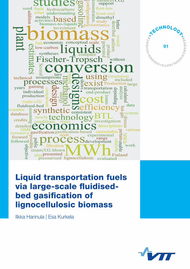
Liquid transportation fuels via large-scale fluidised-bed gasification of lignocellulosic biomass
With the objective of gaining a better understanding of the system design trade-offs and economics that pertain to biomass-to-liquids processes, 20 individual BTL plant designs were evaluated based on their technical and economic performance. The investigation was focused on gasification-based processes that enable the conversion of biomass to methanol, dimethyl ether, Fischer-Tropsch liquids or synthetic gasoline at a large (300 MWth of biomass) scale. The biomass conversion technology was based on pressurised steam/O2-blown fluidised-bed gasification, followed by hot-gas filtration and catalytic conversion of hydrocarbons and tars. This technology has seen extensive development and demonstration activities in Finland during the recent years and newly generated experimental data has been incorporated into the simulation models. Our study included conceptual design issues, process descriptions, mass and energy balances and production cost estimates.
Liquid transportation fuels via large-scale fluidised-bed gasification of lignocellulosic biomassIlkka Hannula | Esa Kurkela
•VISIONS•S
CIE
NC
E•T
ECHNOLOGY•R
ES
EA
RC
HHIGHLIGHTS
91

VTT TECHNOLOGY 91
Liquid transportation fuels via large-scale fluidised-bed gasification of lignocellulosic biomass Ilkka Hannula and Esa Kurkela VTT Technical Research Centre of Finland
ISBN 978-951-38-7978-5 (Soft back ed.) ISBN 978-951-38-7979-2 (URL: http://www.vtt.fi/publications/index.jsp)
VTT Technology 91
ISSN-L 2242-1211 ISSN 2242-1211 (Print) ISSN 2242-122X (Online)
Copyright © VTT 2013
JULKAISIJA – UTGIVARE – PUBLISHER
VTT PL 1000 (Tekniikantie 4 A, Espoo) 02044 VTT Puh. 020 722 111, faksi 020 722 7001
VTT PB 1000 (Teknikvägen 4 A, Esbo) FI-02044 VTT Tfn +358 20 722 111, telefax +358 20 722 7001
VTT Technical Research Centre of Finland P.O. Box 1000 (Tekniikantie 4 A, Espoo) FI-02044 VTT, Finland Tel. +358 20 722 111, fax + 358 20 722 7001
Kopijyvä Oy, Kuopio 2013
3
Liquid transportation fuels via large-scale fluidised-bed gasification of lignocellulosic biomass Liikenteen biopolttoaineiden valmistus metsätähteistä leijukerroskaasutuksen avulla. Ilkka Hannula & Esa Kurkela. Espoo 2013. VTT Technology 91. 114 p. + app. 3 p.
Abstract With the objective of gaining a better understanding of the system design trade-offs and economics that pertain to biomass-to-liquids processes, 20 individual BTL plant designs were evaluated based on their technical and economic performance. The investigation was focused on gasification-based processes that enable the conversion of biomass to methanol, dimethyl ether, Fischer-Tropsch liquids or synthetic gasoline at a large (300 MWth of biomass) scale. The biomass conver-sion technology was based on pressurised steam/O2-blown fluidised-bed gasifica-tion, followed by hot-gas filtration and catalytic conversion of hydrocarbons and tars. This technology has seen extensive development and demonstration activi-ties in Finland during the recent years and newly generated experimental data has been incorporated into the simulation models. Our study included conceptual design issues, process descriptions, mass and energy balances and production cost estimates.
Several studies exist that discuss the overall efficiency and economics of bio-mass conversion to transportation liquids, but very few studies have presented a detailed comparison between various syntheses using consistent process designs and uniform cost database. In addition, no studies exist that examine and compare BTL plant designs using the same front-end configuration as described in this work.
Our analysis shows that it is possible to produce sustainable low-carbon fuels from lignocellulosic biomass with first-law efficiency in the range of 49.6–66.7% depending on the end-product and process conditions. Production cost estimates were calculated assuming Nth plant economics and without public investment support, CO2 credits or tax assumptions. They are 58–65 €/MWh for methanol, 58 –66 €/MWh for DME, 64–75 €/MWh for Fischer-Tropsch liquids and 68–78 €/MWh for synthetic gasoline.
Keywords biomass, biofuels, gasification, methanol, DME, Fischer-Tropsch, MTG
4
Liikenteen biopolttoaineiden valmistus metsätähteistä leijukerros-kaasutuksen avulla
Liquid transportation fuels via large-scale fluidised-bed gasification of lignocellulosic bio-mass. Ilkka Hannula & Esa Kurkela. Espoo 2012. VTT Technology 91. 114 s. + liitt. 3 s.
Tiivistelmä Julkaisussa tarkastellaan metsätähteen kaasutukseen perustuvien liikenteen biopolt-toaineiden tuotantolaitosten toteutusvaihtoehtoja ja arvioidaan näiden vaikutuksia neljän eri lopputuotteen – metanoli, dimetyylieetteri (DME), Fischer-Tropsch-nesteet ja synteettinen bensiini (MTG) – kannalta. Arviointien perustaksi valittiin Suomessa viime vuosina kehitetty prosessi, joka perustuu paineistettuun leijukerroskaasutuk-seen, kaasun kuumasuodatukseen sekä katalyyttiseen tervojen ja hiilivetyjen refor-mointiin. Kaasutusprosessin perusvaihtoehdossa puun kaasutus tapahtuu 5 barin paineessa, minkä jälkeen kaasuttimesta poistuva raakakaasu jäähdytetään 550 °C:n lämpötilaan ja suodatetaan ennen sen johtamista reformeriin, jossa kaasun lämpöti-la jälleen nousee osittaispolton takia yli 900 °C:seen. Tämän perusprosessin toimi-vuus on demonstroitu VTT:llä vuosina 2007–2011 toteutetuissa pitkäkestoisissa PDU-kokoluokan koeajoissa sekä teollisella pilottilaitoksella. Tässä julkaisussa esi-tettyjen tarkastelujen kohteena oli kaikissa tapauksissa suurikokoinen tuotantolaitos, jonka metsätähteen käyttö vastasi saapumistilassaan 300 MW:n tehoa.
Julkaisun tulosten perusteella puumaisesta biomassasta on mahdollista tuottaa uusiutuvia biopolttonesteitä 50–67 %:n energiahyötysuhteella, lopputuotteesta ja prosessiolosuhteista riippuen. Korkein polttoaineen tuotannon hyötysuhde saavute-taan metanolin ja DME:n valmistuksessa. Mikäli myös sivutuotteena syntyvä lämpö-energia pystytään hyödyntämään esimerkiksi kaukolämpönä, nousee biomassan käytön kokonaishyötysuhde 74–80 %:n tasolle. Parhaillaan kehitystyön kohteena oleva kaasun suodatuslämpötilan nosto perusprosessin 550 °C:sta 850 °C:seen parantaisi polttonesteen tuotannon hyötysuhdetta 5–6 prosenttiyksikköä.
Kaupalliseen teknologiaan perustuvien tuotantokustannusarvioiden laskentaole-tuksissa ei huomioitu julkista tukea, päästökauppahyötyjä tai verohelpotuksia. Eri prosessivaihtoehtojen tuotantokustannuksiksi arvioitiin 58–65 €/MWh metanolille, 58–66 €/MWh DME:lle, 64–75 €/MWh Fischer-Tropsch-nesteille ja 68–78 €/MWh synteettiselle polttonesteelle. Korkeimmat tuotantokustannukset ovat kaasutuspro-sessin perusvaihtoehdolle ja tapauksille, joissa sivutuotelämmölle ei ole muuta hyö-tykäyttöä kuin biomassan kuivaus ja lauhdesähkön tuotanto. Alhaisimmat kustan-nukset taas saavutetaan kaukolämpöintegroiduilla laitoksilla, joissa kaasun suodatus tapahtuu korkeassa lämpötilassa. Tuotteiden kustannusarviot ovat lähellä nykyisten raakaöljypohjaisten tuotteiden verotonta hintaa, eivätkä kaupalliset laitokset sen vuoksi vaatisi merkittäviä julkisia tukia tullakseen kannattaviksi. Sen sijaan ensim-mäiset uraauurtavat tuotantolaitokset ovat oletettavasti merkittävästi tässä esitettyjä arvioita kalliimpia, minkä vuoksi teknologian kaupallistuminen edellyttää ensimmäis-ten laitosten osalta merkittävää julkista tukea.
Avainsanat biomass, biofuels, gasification, methanol, DME, Fischer-Tropsch, MTG
1. Introduction
5
Preface This work was carried out in the project “Biomassan kaasutukseen perustuvat alkoholipolttoaineet – Prosessiarvioinnit”, which was funded by Tekes – the Finn-ish Funding Agency for Technology and Innovation, together with VTT Technical Research Centre of Finland. The duration of the project was 1.8.2010–31.6.2012 including a 12 month research visit to the Energy Systems Analysis Group of Princeton University, NJ, USA.
1. Introduction
6
Contents Abstract ........................................................................................................... 3
Tiivistelmä ....................................................................................................... 4
Preface ............................................................................................................. 5
1. Introduction ............................................................................................... 9
2. Technology overview .............................................................................. 14 2.1 Solid biomass conversion & hot-gas cleaning .................................... 15 2.2 Synthesis gas conditioning ................................................................ 18 2.3 Synthesis island ............................................................................... 20
3. Auxiliary equipment design .................................................................... 22 3.1 Biomass pretreatment, drying and feeding equipment ........................ 22 3.2 Air separation unit ............................................................................. 24 3.3 Auxiliary boiler .................................................................................. 25 3.4 Steam cycle...................................................................................... 27 3.5 Compression of the separated CO2 ................................................... 29
4. Case designs and front-end results ........................................................ 30 4.1 Case designs ................................................................................... 30 4.2 Front-end mass and energy balances ................................................ 34
5. Process economics ................................................................................. 36 5.1 Cost estimation methodology ............................................................ 36 5.2 Capital cost estimates ....................................................................... 37 5.3 Feedstock cost estimation ................................................................. 40
6. Methanol synthesis design and results .................................................. 44 6.1 Introduction ...................................................................................... 44 6.2 Synthesis design .............................................................................. 46 6.3 Mass and energy balances ............................................................... 48 6.4 Capital and production cost estimates ............................................... 54
1. Introduction
7
7. Dimethyl ether synthesis design and results ......................................... 57 7.1 Introduction ...................................................................................... 57 7.2 Synthesis design .............................................................................. 58 7.3 Mass and energy balances ............................................................... 60 7.4 Capital and production cost estimates ............................................... 65
8. Fischer-Tropsch synthesis design and results ...................................... 68 8.1 Introduction ...................................................................................... 68 8.2 Synthesis design .............................................................................. 71 8.3 Product recovery and upgrade design ............................................... 73 8.4 Mass and energy balances ............................................................... 74 8.5 Capital and production cost estimates ............................................... 79
9. Methanol-to-gasoline synthesis design and results ............................... 82 9.1 Introduction ...................................................................................... 82 9.2 Synthesis design .............................................................................. 83 9.3 Mass and energy balances ............................................................... 85 9.4 Capital and production cost estimates ............................................... 90
10. Summary of results and sensitivity analysis .......................................... 93
11. Discussion ............................................................................................ 101
Acknowledgements ..................................................................................... 106
References ................................................................................................... 107
Appendix A: Summary of process design parameters

1. Introduction
8
1. Introduction
9
1. Introduction
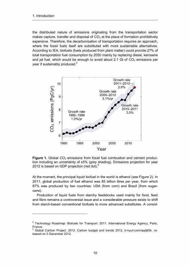
The long-run trend of sustained economic growth has provided economic prosperi-ty and well-being for a large portion of the world’s population. The advancement of material prosperity has been closely linked with a growing demand for energy, which has been largely satisfied by combustion of fossil fuels. As a result, sub-stantial amounts of greenhouse gases and carcinogenic compounds have been released to the atmosphere1 (see Figure 1) causing increased environmental stresses for our planet’s ecosystem, most notably in the form of global warming.
Carbon dioxide (CO2) emissions are the largest contributor to long-term climate change2 urging the development of more sustainable energy conversion process-es characterised by low net carbon emissions. In 2010, the generation of electrici-ty and heat was responsible of 41% of global CO2 emissions.3 The remainder came from direct use of fossil fuels in distributed applications such as transporta-tion and residencies as well as industrial applications. According to IEA, transpor-tation sector is the second largest source of atmospheric carbon, causing nearly one quarter of global energy-related CO2 emissions. 4 Thus, it is clear that a wide-spread decarbonisation of transportation needs to be an integral part of any seri-ous solution to global warming.
For large point source emitters of CO2, such as stationary electric power gener-ators, a likely solution for decarbonisation would be the capture and sequestration of carbon dioxide emissions before they are released to atmosphere. However,
1 Le Quéré, C., Andres, R. J., Boden, T., Conway, T., Houghton, R. A., House, J. I., Marland, G., Peters, G. P., van der Werf, G., Ahlström, A., Andrew, R. M., Bopp, L., Canadell, J. G., Ciais, P., Doney, S. C., Enright, C., Friedlingstein, P., Huntingford, C., Jain, A. K., Jourdain, C., Kato, E., Keeling, R., Levis, S., Levy, P., Lomas, M., Poulter, B., Raupach, M. R., Schwinger, J., Sitch, S., Stocker, B. D., Viovy, N., Zaehle, S., and Zeng, N. (2012) The global carbon budget 1959–2011. Earth System Science Data-Discussions (manuscript under review) 5: 1107–1157. 2 Peters, G., Andrew, R., Boden, T., Canadell, J., Ciais, P., Le Quéré, C. Marland, M., Raupach, M., Wilson, C. 2012. The challenge to keep global warming below two degrees. Nature Climate Change. 3 IEA statistics. 2012. CO2 Emissions from fuel combustion, highlights, International Energy Agency, tinyurl.com/6vz25nl 4 Transport, Energy and CO2: Moving toward Sustainability. 2009. International Energy Agency, ISBN: 978-92-64-07316-6, tinyurl.com/3td6vso
1. Introduction
10
the distributed nature of emissions originating from the transportation sector makes capture, transfer and disposal of CO2 at the place of formation prohibitively expensive. Therefore, the decarbonisation of transportation requires an approach, where the fossil fuels itself are substituted with more sustainable alternatives. According to IEA, biofuels (fuels produced from plant matter) could provide 27% of total transportation fuel consumption by 2050 mainly by replacing diesel, kerosene and jet fuel, which would be enough to avoid about 2.1 Gt of CO2 emissions per year if sustainably produced.5
Figure 1. Global CO2 emissions from fossil fuel combustion and cement produc-tion including an uncertainty of ±5% (grey shading). Emissions projection for year 2012 is based on GDP projection (red dot).6
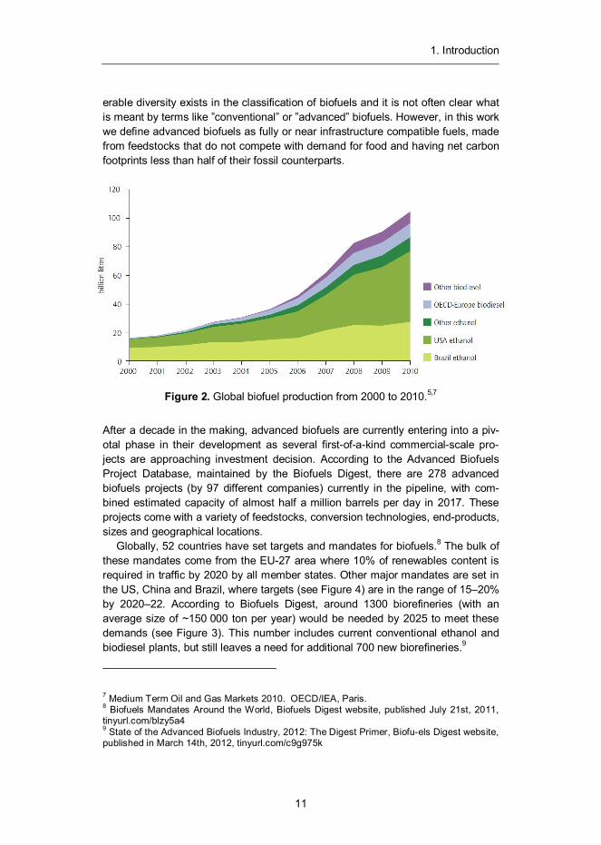
At the moment, the principal liquid biofuel in the world is ethanol (see Figure 2). In 2011, global production of fuel ethanol was 85 billion litres per year, from which 87% was produced by two countries: USA (from corn) and Brazil (from sugar-cane).
Production of liquid fuels from starchy feedstocks used mainly for food, feed and fibre remains a controversial issue and a considerable pressure exists to shift from starch-based conventional biofuels to more advanced substitutes. A consid-
5 Technology Roadmap: Biofuels for Transport. 2011. International Energy Agency, Paris, France. 6 Global Carbon Project. 2012. Carbon budget and trends 2012, ti-nyurl.com/aqdj65k, re-leased on 3 December 2012.
1. Introduction
11
erable diversity exists in the classification of biofuels and it is not often clear what is meant by terms like ”conventional” or ”advanced” biofuels. However, in this work we define advanced biofuels as fully or near infrastructure compatible fuels, made from feedstocks that do not compete with demand for food and having net carbon footprints less than half of their fossil counterparts.
Figure 2. Global biofuel production from 2000 to 2010.5,7
After a decade in the making, advanced biofuels are currently entering into a piv-otal phase in their development as several first-of-a-kind commercial-scale pro-jects are approaching investment decision. According to the Advanced Biofuels Project Database, maintained by the Biofuels Digest, there are 278 advanced biofuels projects (by 97 different companies) currently in the pipeline, with com-bined estimated capacity of almost half a million barrels per day in 2017. These projects come with a variety of feedstocks, conversion technologies, end-products, sizes and geographical locations.
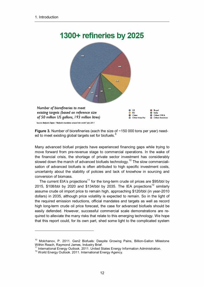
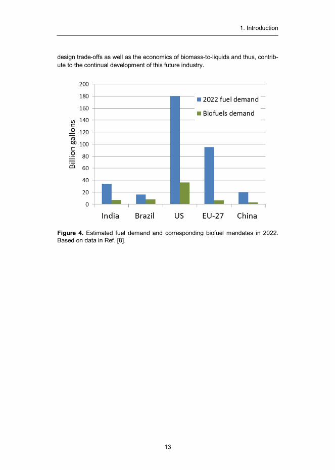
Globally, 52 countries have set targets and mandates for biofuels.8 The bulk of these mandates come from the EU-27 area where 10% of renewables content is required in traffic by 2020 by all member states. Other major mandates are set in the US, China and Brazil, where targets (see Figure 4) are in the range of 15–20% by 2020–22. According to Biofuels Digest, around 1300 biorefineries (with an average size of ~150 000 ton per year) would be needed by 2025 to meet these demands (see Figure 3). This number includes current conventional ethanol and biodiesel plants, but still leaves a need for additional 700 new biorefineries.9
7 Medium Term Oil and Gas Markets 2010. OECD/IEA, Paris. 8 Biofuels Mandates Around the World, Biofuels Digest website, published July 21st, 2011, tinyurl.com/blzy5a4 9 State of the Advanced Biofuels Industry, 2012: The Digest Primer, Biofu-els Digest website, published in March 14th, 2012, tinyurl.com/c9g975k
1. Introduction
12
Figure 3. Number of biorefineries (each the size of ~150 000 tons per year) need-ed to meet existing global targets set for biofuels.8
Many advanced biofuel projects have experienced financing gaps while trying to move forward from pre-revenue stage to commercial operations. In the wake of the financial crisis, the shortage of private sector investment has considerably slowed down the march of advanced biofuels technology.10 The slow commerciali-sation of advanced biofuels is often attributed to high specific investment costs, uncertainty about the stability of policies and lack of knowhow in sourcing and conversion of biomass.
The current EIA’s projections11 for the long-term crude oil prices are $95/bbl by 2015, $108/bbl by 2020 and $134/bbl by 2035. The IEA projections12 similarly assume crude oil import price to remain high, approaching $120/bbl (in year-2010 dollars) in 2035, although price volatility is expected to remain. So in the light of the required emission reductions, official mandates and targets as well as record high long-term crude oil price forecast, the case for advanced biofuels should be easily defended. However, successful commercial scale demonstrations are re-quired to alleviate the many risks that relate to this emerging technology. We hope that this report could, for its own part, shed some light to the complicated system
10 Molchanov, P. 2011. Gen2 Biofuels: Despite Growing Pains, Billion-Gallon Milestone Within Reach, Raymond James, Industry Brief. 11 International Energy Outlook. 2011. United States Energy Information Administration. 12 World Energy Outlook. 2011. International Energy Agency.
1. Introduction
13
design trade-offs as well as the economics of biomass-to-liquids and thus, contrib-ute to the continual development of this future industry.
Figure 4. Estimated fuel demand and corresponding biofuel mandates in 2022. Based on data in Ref. [8].
2. Technology overview
14
2. Technology overview
Large-scale production of synthetic fuels from biomass requires a fairly complex process that combines elements from power plants, refineries and wood-processing industry. Most of the components needed to build a biomass-to-liquids (BTL) plant are already commercially mature, making near-term deployment of such plants possible. However, conversion of solid biomass into clean, nitrogen-free gas, requires some advanced technologies that, although already demon-strated at a pre-commercial scale, are not yet fully commercialised.
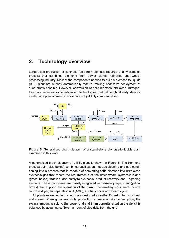
Figure 5. Generalised block diagram of a stand-alone biomass-to-liquids plant examined in this work.
A generalised block diagram of a BTL plant is shown in Figure 5. The front-end process train (blue boxes) combines gasification, hot-gas cleaning and gas condi-tioning into a process that is capable of converting solid biomass into ultra-clean synthesis gas that meets the requirements of the downstream synthesis island (green boxes) that includes catalytic synthesis, product recovery and upgrading sections. These processes are closely integrated with auxiliary equipment (yellow boxes) that support the operation of the plant. The auxiliary equipment include biomass dryer, air separation unit (ASU), auxiliary boiler and steam cycle.
All plants examined in this work are designed as self-sufficient in terms of heat and steam. When gross electricity production exceeds on-site consumption, the excess amount is sold to the power grid and in an opposite situation the deficit is balanced by acquiring sufficient amount of electricity from the grid.
2. Technology overview
15
It should be emphasised that when actual BTL plants are built, it is often advis-able to integrate them with existing processes to minimise capital footprint and to ensure efficient utilisation and exchange of heat and steam. However, as integra-tion solutions are highly case specific, the design of a representative plant configu-ration is difficult. “Stand-alone” plant was therefore adopted as a basis for all stud-ied process configurations.
2.1 Solid biomass conversion & hot-gas cleaning
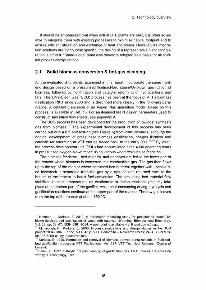
All the evaluated BTL plants, examined in this report, incorporate the same front-end design based on a pressurised fluidised-bed steam/O2-blown gasification of biomass, followed by hot-filtration and catalytic reforming of hydrocarbons and tars. This Ultra-Clean Gas (UCG) process has been at the focus of VTT’s biomass gasification R&D since 2006 and is described more closely in the following para-graphs. A detailed discussion of an Aspen Plus simulation model, based on this process, is available in Ref. 13. For an itemised list of design parameters used to construct simulation flow sheets, see appendix A.
The UCG process has been developed for the production of low-cost synthesis gas from biomass.14 The experimental development of this process has been carried out with a 0.5 MW test-rig (see Figure 6) from 2006 onwards, although the original development of pressurised biomass gasification, hot-gas filtration and catalytic tar reforming at VTT can be traced back to the early 90’s.15,16 By 2012, the process development unit (PDU) had accumulated circa 4000 operating hours in pressurised oxygen-blown mode using various wood residues as feedstock.
The biomass feedstock, bed material and additives are fed to the lower part of the reactor where biomass is converted into combustible gas. The gas then flows up to the top of the reactor where entrained bed material together with unconvert-ed feedstock is separated from the gas by a cyclone and returned back to the bottom of the reactor to boost fuel conversion. The circulating bed material flow stabilizes reactor temperatures as exothermic oxidation reactions primarily take place at the bottom part of the gasifier, while heat-consuming drying, pyrolysis and gasification reactions continue at the upper part of the reactor. The raw gas leaves from the top of the reactor at about 850 °C.
13 Hannula, I., Kurkela, E. 2012. A parametric modelling study for pressurised steam/O2-blown fluidised-bed gasification of wood with catalytic reforming, Biomass and Bioenergy, Vol. 38, pp. 58–67, ISSN 0961-9534, A post-print is available via: tinyurl.com/c6tcqzq 14 McKeough, P., Kurkela, E. 2008. Process evaluations and design studies in the UCG project 2004–2007. Espoo, VTT. 45 p. VTT Tiedotteita – Research Notes; 2434. ISBN 978-951-38-7209-0; tinyurl.com/bre4cdx 15 Kurkela, E. 1996. Formation and removal of biomass-derived conta-minants in fluidized-bed gasification processes VTT Publications, Vol. 287. VTT Technical Research Centre of Finland. 16 Simell, P. 1997. Catalytic hot gas cleaning of gasification gas. Ph.D. the-sis, Helsinki Uni-versity of Technology, TKK.
2. Technology overview
16
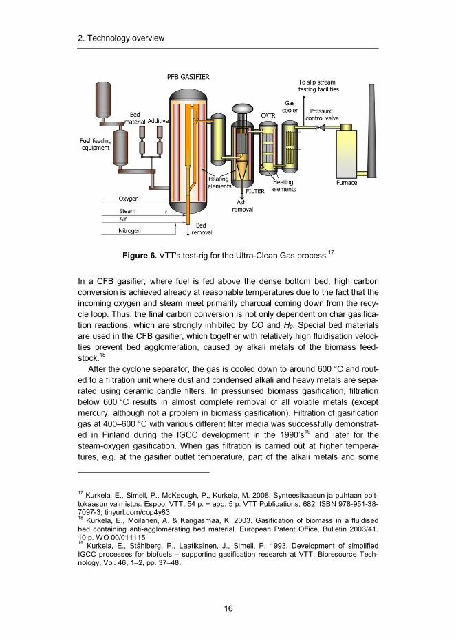
Figure 6. VTT's test-rig for the Ultra-Clean Gas process.17
In a CFB gasifier, where fuel is fed above the dense bottom bed, high carbon conversion is achieved already at reasonable temperatures due to the fact that the incoming oxygen and steam meet primarily charcoal coming down from the recy-cle loop. Thus, the final carbon conversion is not only dependent on char gasifica-tion reactions, which are strongly inhibited by CO and H2. Special bed materials are used in the CFB gasifier, which together with relatively high fluidisation veloci-ties prevent bed agglomeration, caused by alkali metals of the biomass feed-stock.18
After the cyclone separator, the gas is cooled down to around 600 °C and rout-ed to a filtration unit where dust and condensed alkali and heavy metals are sepa-rated using ceramic candle filters. In pressurised biomass gasification, filtration below 600 °C results in almost complete removal of all volatile metals (except mercury, although not a problem in biomass gasification). Filtration of gasification gas at 400–600 °C with various different filter media was successfully demonstrat-ed in Finland during the IGCC development in the 1990’s19 and later for the steam-oxygen gasification. When gas filtration is carried out at higher tempera-tures, e.g. at the gasifier outlet temperature, part of the alkali metals and some
17 Kurkela, E., Simell, P., McKeough, P., Kurkela, M. 2008. Synteesikaasun ja puhtaan polt-tokaasun valmistus. Espoo, VTT. 54 p. + app. 5 p. VTT Publications; 682, ISBN 978-951-38-7097-3; tinyurl.com/cop4y83 18 Kurkela, E., Moilanen, A. & Kangasmaa, K. 2003. Gasification of biomass in a fluidised bed containing anti-agglomerating bed material. European Patent Office, Bulletin 2003/41. 10 p. WO 00/011115 19 Kurkela, E., Ståhlberg, P., Laatikainen, J., Simell, P. 1993. Development of simplified IGCC processes for biofuels – supporting gasification research at VTT. Bioresource Tech-nology, Vol. 46, 1–2, pp. 37–48.
2. Technology overview
17
heavy metals will remain in gaseous form. This may lead to catalyst poisoning or deposit formation on heat exchanger surfaces when the gas is cooled down after reforming. Further R&D is being carried out by VTT on issues related to high-temperature filtration.
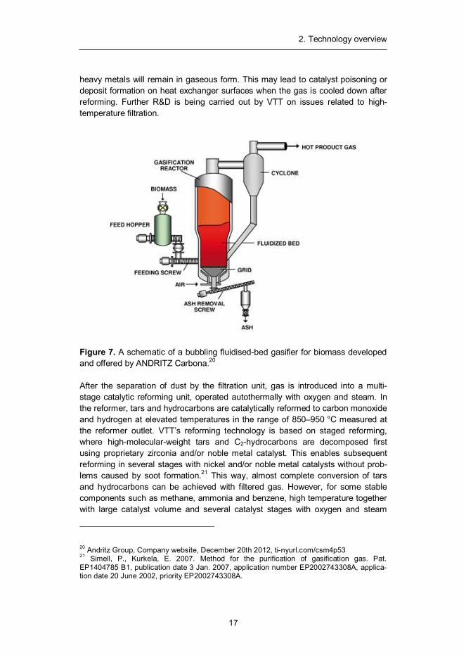
Figure 7. A schematic of a bubbling fluidised-bed gasifier for biomass developed and offered by ANDRITZ Carbona.20 After the separation of dust by the filtration unit, gas is introduced into a multi-stage catalytic reforming unit, operated autothermally with oxygen and steam. In the reformer, tars and hydrocarbons are catalytically reformed to carbon monoxide and hydrogen at elevated temperatures in the range of 850–950 °C measured at the reformer outlet. VTT’s reforming technology is based on staged reforming, where high-molecular-weight tars and C2-hydrocarbons are decomposed first using proprietary zirconia and/or noble metal catalyst. This enables subsequent reforming in several stages with nickel and/or noble metal catalysts without prob-lems caused by soot formation.21 This way, almost complete conversion of tars and hydrocarbons can be achieved with filtered gas. However, for some stable components such as methane, ammonia and benzene, high temperature together with large catalyst volume and several catalyst stages with oxygen and steam
20 Andritz Group, Company website, December 20th 2012, ti-nyurl.com/csm4p53 21 Simell, P., Kurkela, E. 2007. Method for the purification of gasification gas. Pat. EP1404785 B1, publication date 3 Jan. 2007, application number EP2002743308A, applica-tion date 20 June 2002, priority EP2002743308A.
2. Technology overview
18
addition is required to achieve complete conversion. The increase in operating pressure increases methane formation in the gasifier making it more difficult to achieve full methane conversion. This effect could be compensated by further increasing the reformer temperature and the number of reformer stages. However, over 1000 °C temperatures at the reformer outlet would lead to high oxygen con-sumption and would not be technically feasible with the present catalyst combina-tions included in VTT’s reforming technology. Consequently, reformer perfor-mance in this report is based on circa 950 °C outlet temperature using catalysts demonstrated in our PDU-scale test trials.
After the reformer, the gas has been pre-cleaned from major biomass-derived impurities that formed during gasification. The H2/CO ratio is now close to equilib-rium as some reforming catalysts (nickel and noble metal) also catalyse water-gas shift reaction. The properties of the gas are now comparable to synthesis gas produced by steam reforming of natural gas, and consequently, much of the re-quired downstream equipment can readily be adapted from existing synthesis gas industry.
2.2 Synthesis gas conditioning
Although a variety of impurities have already been removed from the gas, some further conditioning is still needed to meet the stringent requirements of the down-stream catalytic synthesis. The stoichiometric requirement of the fuel synthesis, in respect to the ratio of H2/CO in the make-up synthesis gas, is usually close to 2. Hydrogen-rich gases are characterised by values above 2 and are typical for indi-rect conversion routes. Values below 2 indicate carbon-rich gases normally ob-tained by conversion routes based on partial oxidation approach.
+ = + = 41,2 kJ/mol (1)
Synthesis gas, generated from forest residues with the kind of process described above, has a H2/CO ratio of about 1.4 at the reformer outlet and needs to be ad-justed to suite the downstream synthesis. This can be achieved by further catalys-ing the water-gas shift reaction (1) in an autothermal reactor filled with sulphur-tolerant cobalt catalyst. To drive the reaction and to suppress catalyst deactiva-tion, steam needs to be added until a minimum steam/CO ratio of 1.8 is achieved at the shift inlet.22 Heat from the slightly exothermic shift reaction dissipates to syngas causing its temperature to rise. To prevent deactivation of the catalyst, outlet temperature needs to be limited to 404 °C, which is controlled by adjusting the inlet temperature.
22 Kaltner, W. Personal communication, Clariant / Süd-Chemie AG, July 9th, 2012.
2. Technology overview
19
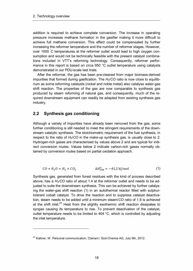
Figure 8. Layout of CO shift arrangement.
In order to avoid excess amount of CO shift, a portion of the feed gas needs to be bypassed around the reactor as shown in Figure 8. The amount of bypass is ad-justed to achieve a desired H2/CO ratio after the gas streams are once again combined. In addition to the CO conversion, sour shift catalysts also convert car-bonyl sulphide (COS), hydrogen cyanide (HCN) and other organic sulphur species to hydrogen sulphide (H2S), a more readily removable form of sulphur for the downstream equipment. To ensure complete hydrolysis of sulphur species, the bypass stream needs to be equipped with a separate hydrolysis reactor. In the CO shift converter the hydrogenation of COS proceeds in parallel with the water-gas reaction according to equation ), while in the separate reactor the COS hydrolysis achieves equilibrium according to equation (3).23 Both reactions have low ap-proach to equilibrium temperatures with satisfactory space velocities using modern catalysts.
H2 + COS = H2S+CO (2)
After the CO shift, syngas needs to be cooled close to ambient temperature before additional compression for the AGR and synthesis. The first syngas cooler lowers the temperature of the gas to 220 °C while simultaneously recovering heat for steam generation. The second cooling step from 220 °C to 40 °C is performed in a two-stage water scrubber to minimise the risk of residual tar condensation on syngas cooler surfaces. The first scrubber unit recovers heat between 220–60 °C which is used for biomass drying. The second scrubber stage lowers temperature further down to 40 °C and the recovered heat is directed to a near-by lake or a sea
23 Supp, E. 1990. How to produce methanol from coal. Springer-Verlag Berlin, Heidelberg.
2. Technology overview
20
(or to cooling towers if no natural source of cooling water is available). Any ammo-nia contained in the gas will be removed by the scrubber. A portion of scrubber water is continuously sent to an on-site water treatment facility, where it is cleaned and used to produce make-up water for the steam system. Formic acid can occa-sionally be rationed to the scrubber to control the pH value of the washing solu-tion.
+ = + (3)
Synthesis catalysts are usually very sensitive to impurities and especially all sul-phur must be removed upstream to avoid catalyst poisoning and deactivation. In addition to sulphur, an upstream removal of CO2 from the syngas is usually rec-ommended to maximise the productivity of downstream synthesis.
After the gas is cooled down to a near-ambient temperature and dried, it is compressed to higher pressure that enables more efficient operation of physical acid gas removal and catalytic synthesis. The pressure is elevated in a multistage centrifugal compressor with an intercooling to 35 °C between stages.
The acid gas removal step is based on Rectisol for all studied process configu-rations. Rectisol is a commercially proven physical washing process that uses chilled methanol as solvent and is able to guarantee a removal of total sulphur to less than 0.1 ppmv.24 After the separation, the acid gas laden solvent can be easi-ly regenerated with combination of flashing and steam. Physical absorption sys-tems are also capable of carrying out a selective removal of components by adapt-ing the solvent flow rate to the solubility coefficients of the gas components.25
2.3 Synthesis island
Synthesis island can be divided into three sub-sections: synthesis loop, product recovery and upgrading. In the synthesis loop, carbon monoxide and hydrogen are converted into desired products by catalysing the wanted and suppressing the unwanted reactions. The amount of synthesis gas that can be turned to products in a single pass of gas through the converter depends on the selection of catalyst and the design and size of the reactor. To boost the production of liquid fuel, un-converted part of the gas can be separated from the formed product and recycled back to the reactor.
A well designed synthesis loop should achieve high conversion and low by-product formation with low catalyst volume and should also recover reaction heat at high temperature level. While the recycle approach does enable high overall conversion, it also leads to increased costs in the form of additional equipment, increased gas flows through the synthesis loop and recirculator’s power consump-
24 Hochgesand, G. (1970) Rectisol and Purisol. Ind. Eng. Chem., 62 (7), 37–43. 25 Weiss, H. 1988. Rectisol wash for purification of partial oxidation gases. Gas Sep. Pur. 2 (4), 171–176.
2. Technology overview
21
tion. Gases such as methane, argon and nitrogen are considered inerts in the synthesis loop and their amount should be minimised as they increase purge gas volume and have adverse effect to the economics.
As described above, a proper design of a synthesis island is an intricate object function to optimise. In our synthesis designs we have aimed to minimise the specific synthesis gas consumption because we expect it to provide reduced feed-stock costs as well as investment savings for the upstream process due to lower gas volumes. This objective can be achieved by maximising synthesis gas effi-ciency:
= 1 ( ) ( )
, (4)
where CO and H2 refer to the molar concentrations of these components in gas. A majority of the formed product can be recovered from the reactor effluent by
means of condensation at synthesis pressure with cooling water at 45 °C. In some instances it might be beneficial to recover also the C1-C2 hydrocarbons to improve carbon efficiency. However, this approach requires the use of cryogenic separa-tion, which comes with cost and extra complexity. Therefore we have decided to exclude it from our syntheses designs.
The design of an upgrading area is highly dependent on the product being pro-duced and ranges from simple distillation approach to a full-blown refinery employ-ing hydrocrackers and treaters. These (and many other) issues are discussed in detail later in the report. For all upgrading areas we assume that the recovery of waste heat is enough to provide the needed utilities, leading to zero net parasitic utilities demand for the area.
3. Auxiliary equipment design
22
3. Auxiliary equipment design
Auxiliary equipment are required to support the operation of a BTL plant and close integration between the main process and auxiliaries is needed to ensure high performance and minimum production costs. The following text discusses tech-nical features adopted in the design of auxiliary systems for this study. An itemised list of process design parameters is available in appendix A.
3.1 Biomass pretreatment, drying and feeding equipment
Feedstock pretreatment is an important part of almost every biomass conversion process. The specific arrangement of a pretreatment chain is dependent on the feed and conversion application, but usually includes at least transfer, storage, chipping, crushing and drying of feedstock. In any event, drying is probably the most challenging of the pretreatment steps.26
Forest residue chips, produced from the residue formed during harvesting of industrial wood, was chosen as feedstock for all examined cases. It includes nee-dles and has higher proportion of bark than chips made out of whole trees. 300 MWth of biomass flows continuously to the dryer at 50 wt% moisture, corre-sponding to a dry matter flow of 1348 metric tons per day. The properties of forest residue chips27 are described in Table 1.
After having considered a variety of drying options, an atmospheric band con-veyor dryer (belt dryer) was chosen for all investigated plant designs. The dryer operates mostly with hot water (90 °C in, 60 °C out), derived from the first cooling stage of the syngas scrubber and from low temperature heat sources of the cata-lytic synthesis. It is used to dry the feedstock from 50 wt% to 15 wt% moisture.
26 Fagernäs, L., Brammer, J. Wilen, C., Lauer, M., Verhoeff, F. 2010. Drying of biomass for second generation synfuel production, Biomass and Bioenergy, Vol. 34(9), pp. 1267–1277, ISSN 0961-9534, 10.1016/j.biombioe.2010.04.005. 27 Wilen, C., Moilanen, A., Kurkela, E. 1996. Biomass feedstock analyses, VTT Publications 282, ISBN 951-38-4940-6
3. Auxiliary equipment design
23
Table 1. Feedstock properties for forest residues chosen as feedstock for all in-vestigated plant designs.27
FEEDSTOCK PROPERTIES Proximate analysis, wt% d.b.* Fixed carbon 19.37 Volatile matter 79.3 Ash 1.33 Ultimate analysis, wt% d.b. Ash 1.33 C 51.3 H 6.10 N 0.40 Cl 0 S 0.02 O (difference) 40.85 HHV, MJ/kg 20.67 Moisture content, wt% 50/15 LHV, MJ/kg 8.60/16.33 Bulk density, kg d.b./m3** Sintering temp. of ash >1000 *wt% d.b. = weight percent dry basis
**1 litre batch, not shaken
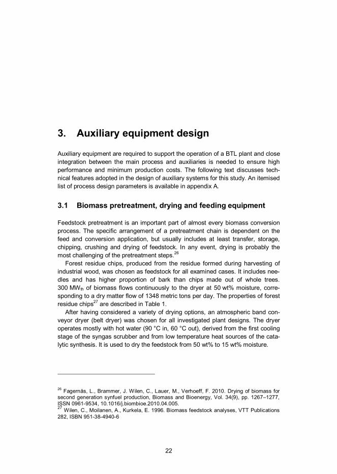
The operating principle of a commercially available SWISS COMBI’s single-stage single-pass biomass belt dryer is illustrated in Figure 9. According to an advertorial brochure28, it can be used to dry biomass down to 8 wt% moisture content, using various low temperature heat sources. One dryer is able to evaporate up to 20 ton of water per hour, and if necessary, multiple dryers can be stacked on top of each other to save floor space. A relatively thin layer of feedstock (2–15 cm) on the belt enables good uniformity of drying.26 All of our plant designs feature belt dryers with a maximum feedstock capacity of 100 MW per unit, operated in a recycle mode having a specific energy consumption of 1100 kWh/tonH2O evaporated. We as-sume 20% of this requirement to be satisfied with low (< 60 °C) temperature heat while the rest is satisfied with district heat with 90/60 °C inlet/outlet temperature. When the combined duty of the scrubber and synthesis falls short from the dryer’s heat requirement, low pressure steam (at 100 °C and 1 bar) is extracted from the turbine to close the heat balance.
28 Metso broschure on KUVO belt dryer: tinyurl.com/cf5dyhv
3. Auxiliary equipment design
24
Figure 9. A schematic of a KUVO belt dryer.28
When the feedstock arrives to the plant site, it needs to be cleaned and crushed to a particle size required by the gasification process. A sufficient storage capacity is also needed to enable continuous plant operation. After the dryer, biomass is fed to the process by a system that consists of an atmospheric storage/weigh silo, lock-hoppers for fuel pressurisation with inert gas to gasifier pressure, a surge hopper, a metering screw and a feeding screw to the gasifier. Bed material is fed through a separate lock-hopper/surge-hopper system to one of the fuel feeding screws. In a commercial plant, three parallel fuel feeding lines are required to enable continuous gasifier output without interruptions.29
Feeding of the dried solid biomass into a pressurised reactor is a technically challenging step, although well designed lock-hopper systems can be considered available for reliable execution. The downside of using lock-hoppers for the feed-stock pressurisation is the relatively high inert gas consumption per unit of energy fed into the process – a result of the low bulk density of biomass. However, an ample supply of inert CO2 is available from the acid gas removal unit situated downstream in the process.
3.2 Air separation unit
Oxygen is required for the generation of nitrogen-free synthesis gas, when gasifi-cation and reforming are based on partial oxidation. A variety of processes exist for the separation of oxygen and nitrogen from air (e.g. adsorption processes,
29 Carbona Inc. 2009. BiGPower D71 Finnish case study report, Project co-founded by the European Commission within the Sixth Framework Pro-gramme, project no. 019761.
3. Auxiliary equipment design
25
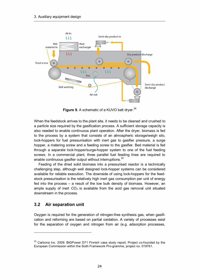
polymeric membranes or ion transportation membranes), but for the production of large quantities (> 20 tons per day) of oxygen and nitrogen at high recoveries and purities, the conventional multi-column cryogenic distillation process still remains as the most cost-effective option.30
Figure 10. Flow scheme of a cryogenic air separation unit.31
In the cryogenic air separation unit (see Figure 10), air is first pressurised and then purified from CO2 and moisture in a molecular sieve unit. The clean compressed air is then precooled against cold product streams, followed by further cooling down to liquefaction temperature by the Joule-Thompson effect. The liquefied air is then separated to its main components in a distillation tower operating between the boiling points of nitrogen and oxygen (-196 °C to -183 °C). Because the boiling point of argon is very similar to that of oxygen, the purity of the oxygen product from a double column unit is limited to around 96%. However, if higher purity oxy-gen is required, argon can also be removed by the addition of a third distillation column yielding a pure argon product.31 All the investigated plant designs feature stand-alone cryogenic air separation unit producing 99.5 mol% oxygen at a 1.05 bar delivery pressure.
3.3 Auxiliary boiler
The electricity consumption of a BTL plant using 300 MWth (LHV) of biomass is typically in the range of 20–30 MWe, depending on the pressure levels of equip-ment and configuration of the synthesis. Roughly half of this consumption can be
30 Smith, A.R., Klosek, J. 2001. A review of air separation technologies and their integration with energy conversion processes, Fuel Processing Technology, Vol. 70(2), pp. 115–134, ISSN 0378-3820. 31 Rackley, S. A. 2010. Carbon Capture and Storage. Elsevier.
3. Auxiliary equipment design
26
satisfied with a steam system that recovers heat from the hot syngas at the gasifi-cation island. The rest needs to be provided with the combination of grid purchas-es and on-site production by combustion of byproducts.
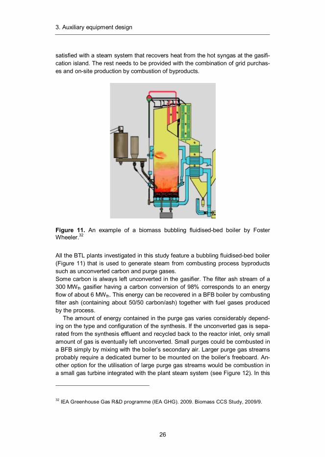
Figure 11. An example of a biomass bubbling fluidised-bed boiler by Foster Wheeler.32
All the BTL plants investigated in this study feature a bubbling fluidised-bed boiler (Figure 11) that is used to generate steam from combusting process byproducts such as unconverted carbon and purge gases. Some carbon is always left unconverted in the gasifier. The filter ash stream of a 300 MWth gasifier having a carbon conversion of 98% corresponds to an energy flow of about 6 MWth. This energy can be recovered in a BFB boiler by combusting filter ash (containing about 50/50 carbon/ash) together with fuel gases produced by the process.
The amount of energy contained in the purge gas varies considerably depend-ing on the type and configuration of the synthesis. If the unconverted gas is sepa-rated from the synthesis effluent and recycled back to the reactor inlet, only small amount of gas is eventually left unconverted. Small purges could be combusted in a BFB simply by mixing with the boiler’s secondary air. Larger purge gas streams probably require a dedicated burner to be mounted on the boiler’s freeboard. An-other option for the utilisation of large purge gas streams would be combustion in a small gas turbine integrated with the plant steam system (see Figure 12). In this
32 IEA Greenhouse Gas R&D programme (IEA GHG). 2009. Biomass CCS Study, 2009/9.
3. Auxiliary equipment design
27
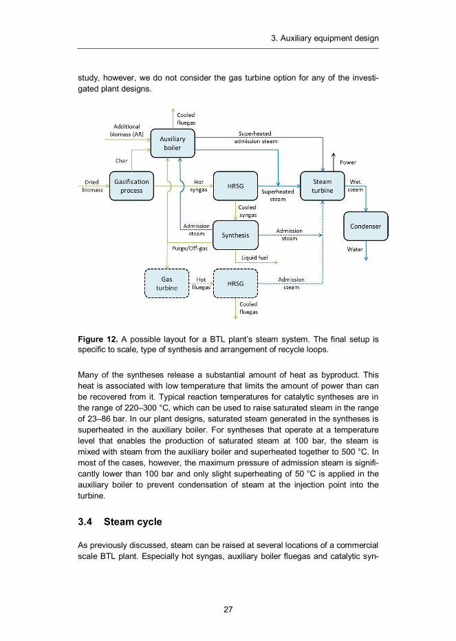
study, however, we do not consider the gas turbine option for any of the investi-gated plant designs.
Figure 12. A possible layout for a BTL plant’s steam system. The final setup is specific to scale, type of synthesis and arrangement of recycle loops.
Many of the syntheses release a substantial amount of heat as byproduct. This heat is associated with low temperature that limits the amount of power than can be recovered from it. Typical reaction temperatures for catalytic syntheses are in the range of 220–300 °C, which can be used to raise saturated steam in the range of 23–86 bar. In our plant designs, saturated steam generated in the syntheses is superheated in the auxiliary boiler. For syntheses that operate at a temperature level that enables the production of saturated steam at 100 bar, the steam is mixed with steam from the auxiliary boiler and superheated together to 500 °C. In most of the cases, however, the maximum pressure of admission steam is signifi-cantly lower than 100 bar and only slight superheating of 50 °C is applied in the auxiliary boiler to prevent condensation of steam at the injection point into the turbine.
3.4 Steam cycle
As previously discussed, steam can be raised at several locations of a commercial scale BTL plant. Especially hot syngas, auxiliary boiler fluegas and catalytic syn-
3. Auxiliary equipment design
28
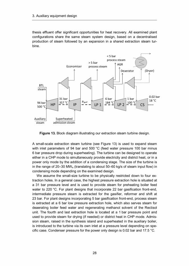
thesis effluent offer significant opportunities for heat recovery. All examined plant configurations share the same steam system design, based on a decentralised production of steam followed by an expansion in a shared extraction steam tur-bine.
Figure 13. Block diagram illustrating our extraction steam turbine design.
A small-scale extraction steam turbine (see Figure 13) is used to expand steam with inlet parameters of 94 bar and 500 °C (feed water pressure 100 bar minus 6 bar pressure drop during superheating). The turbine can be designed to operate either in a CHP mode to simultaneously provide electricity and district heat, or in a power only mode by the addition of a condensing stage. The size of the turbine is in the range of 20–30 MWe (translating to about 50–60 kg/s of steam input flow) in condensing mode depending on the examined design.
We assume the small-size turbine to be physically restricted down to four ex-traction holes. In a general case, the highest pressure extraction hole is situated at a 31 bar pressure level and is used to provide steam for preheating boiler feed water to 220 °C. For plant designs that incorporate 22 bar gasification front-end, intermediate pressure steam is extracted for the gasifier, reformer and shift at 23 bar. For plant designs incorporating 5 bar gasification front-end, process steam is extracted at a 6 bar low pressure extraction hole, which also serves steam for deaerating boiler feed water and regenerating methanol solvent of the Rectisol unit. The fourth and last extraction hole is located at a 1 bar pressure point and used to provide steam for drying (if needed) or district heat in CHP mode. Admis-sion steam, raised in the synthesis island and superheated in the auxiliary boiler, is introduced to the turbine via its own inlet at a pressure level depending on spe-cific case. Condenser pressure for the power only design is 0.02 bar and 17.5 °C.
3. Auxiliary equipment design
29
3.5 Compression of the separated CO2
A BTL process can also be designed to capture and sequestrate (CCS) the CO2 that is constantly formed during biomass conversion. In this kind of Bio-CCS de-sign, carbon, acquired from ambient air during the growth of biomass, ends up sequestered below ground and is thus permanently removed from atmosphere. As a result, biofuels produced with such a system can have even strongly negative life-cycle emissions.
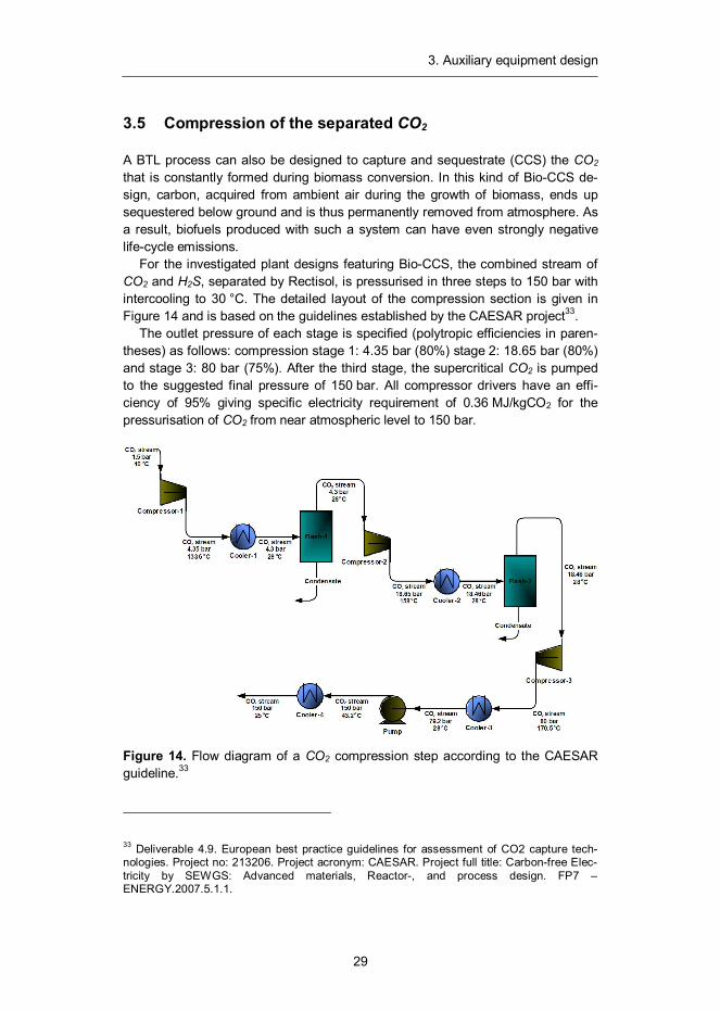
For the investigated plant designs featuring Bio-CCS, the combined stream of CO2 and H2S, separated by Rectisol, is pressurised in three steps to 150 bar with intercooling to 30 °C. The detailed layout of the compression section is given in Figure 14 and is based on the guidelines established by the CAESAR project33.
The outlet pressure of each stage is specified (polytropic efficiencies in paren-theses) as follows: compression stage 1: 4.35 bar (80%) stage 2: 18.65 bar (80%) and stage 3: 80 bar (75%). After the third stage, the supercritical CO2 is pumped to the suggested final pressure of 150 bar. All compressor drivers have an effi-ciency of 95% giving specific electricity requirement of 0.36 MJ/kgCO2 for the pressurisation of CO2 from near atmospheric level to 150 bar.
Figure 14. Flow diagram of a CO2 compression step according to the CAESAR guideline.33
33 Deliverable 4.9. European best practice guidelines for assessment of CO2 capture tech-nologies. Project no: 213206. Project acronym: CAESAR. Project full title: Carbon-free Elec-tricity by SEWGS: Advanced materials, Reactor-, and process design. FP7 – ENERGY.2007.5.1.1.
4. Case designs and front-end results
30
4. Case designs and front-end results
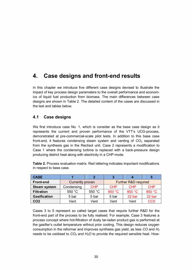
In this chapter we introduce five different case designs devised to illustrate the impact of key process design parameters to the overall performance and econom-ics of liquid fuel production from biomass. The main differences between case designs are shown in Table 2. The detailed content of the cases are discussed in the text and tables below.
4.1 Case designs
We first introduce case No. 1, which is consider as the base case design as it represents the current and proven performance of the VTT’s UCG-process, demonstrated at pre-commercial-scale pilot tests. In addition to this base case front-end, it features condensing steam system and venting of CO2, separated from the synthesis gas in the Rectisol unit. Case 2 represents a modification to Case 1 where the condensing turbine is replaced with a back-pressure design producing district heat along with electricity in a CHP mode.
Table 2. Process evaluation matrix. Red lettering indicates important modifications in respect to base case.
CASE 1 2 3 4 5 Front-end Currently proven Further R&D required Steam system Condensing CHP CHP CHP CHP Filtration 550 °C 550 °C 850 °C 850 °C 850 °C Gasification 5 bar 5 bar 5 bar 22 bar 22 bar CO2 Vent Vent Vent Vent CCS
Cases 3 to 5 represent so called target cases that require further R&D for the front-end part of the process to be fully realised. For example, Case 3 features a process concept where hot-filtration of dusty tar-laden product gas is performed at the gasifier’s outlet temperature without prior cooling. This design reduces oxygen consumption in the reformer and improves synthesis gas yield, as less CO and H2 needs to be oxidised to CO2 and H2O to provide the required sensible heat. How-
4. Case designs and front-end results
31
ever, the challenges of this concept are related to the fate of alkali metals in the reformer and gas coolers as well as soot formation on the filter dust cake, which may prevent efficient filtration.
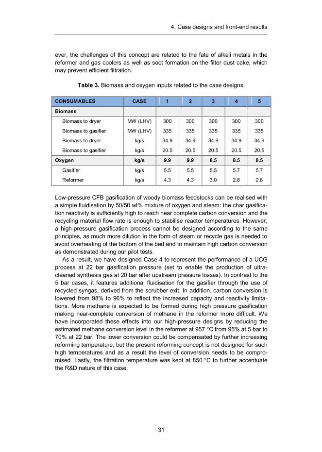
Table 3. Biomass and oxygen inputs related to the case designs.
CONSUMABLES CASE 1 2 3 4 5
Biomass
Biomass to dryer MW (LHV) 300 300 300 300 300
Biomass to gasifier MW (LHV) 335 335 335 335 335
Biomass to dryer kg/s 34.9 34.9 34.9 34.9 34.9
Biomass to gasifier kg/s 20.5 20.5 20.5 20.5 20.5
Oxygen kg/s 9.9 9.9 8.5 8.5 8.5
Gasifier kg/s 5.5 5.5 5.5 5.7 5.7
Reformer kg/s 4.3 4.3 3.0 2.8 2.8
Low-pressure CFB gasification of woody biomass feedstocks can be realised with a simple fluidisation by 50/50 wt% mixture of oxygen and steam: the char gasifica-tion reactivity is sufficiently high to reach near complete carbon conversion and the recycling material flow rate is enough to stabilise reactor temperatures. However, a high-pressure gasification process cannot be designed according to the same principles, as much more dilution in the form of steam or recycle gas is needed to avoid overheating of the bottom of the bed and to maintain high carbon conversion as demonstrated during our pilot tests.
As a result, we have designed Case 4 to represent the performance of a UCG process at 22 bar gasification pressure (set to enable the production of ultra-cleaned synthesis gas at 20 bar after upstream pressure losses). In contrast to the 5 bar cases, it features additional fluidisation for the gasifier through the use of recycled syngas, derived from the scrubber exit. In addition, carbon conversion is lowered from 98% to 96% to reflect the increased capacity and reactivity limita-tions. More methane is expected to be formed during high pressure gasification making near-complete conversion of methane in the reformer more difficult. We have incorporated these effects into our high-pressure designs by reducing the estimated methane conversion level in the reformer at 957 °C from 95% at 5 bar to 70% at 22 bar. The lower conversion could be compensated by further increasing reforming temperature, but the present reforming concept is not designed for such high temperatures and as a result the level of conversion needs to be compro-mised. Lastly, the filtration temperature was kept at 850 °C to further accentuate the R&D nature of this case.
4. Case designs and front-end results
32
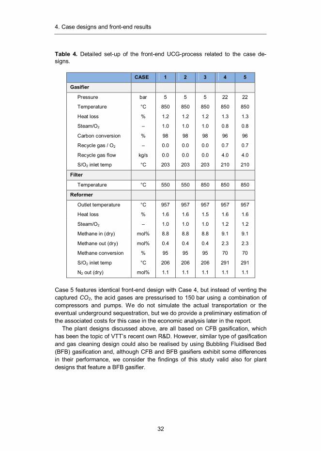
Table 4. Detailed set-up of the front-end UCG-process related to the case de-signs.
CASE 1 2 3 4 5
Gasifier
Pressure bar 5 5 5 22 22
Temperature °C 850 850 850 850 850
Heat loss % 1.2 1.2 1.2 1.3 1.3
Steam/O2 – 1.0 1.0 1.0 0.8 0.8
Carbon conversion % 98 98 98 96 96
Recycle gas / O2 – 0.0 0.0 0.0 0.7 0.7
Recycle gas flow kg/s 0.0 0.0 0.0 4.0 4.0
S/O2 inlet temp °C 203 203 203 210 210
Filter
Temperature °C 550 550 850 850 850
Reformer
Outlet temperature °C 957 957 957 957 957
Heat loss % 1.6 1.6 1.5 1.6 1.6
Steam/O2 – 1.0 1.0 1.0 1.2 1.2
Methane in (dry) mol% 8.8 8.8 8.8 9.1 9.1
Methane out (dry) mol% 0.4 0.4 0.4 2.3 2.3
Methane conversion % 95 95 95 70 70
S/O2 inlet temp °C 206 206 206 291 291
N2 out (dry) mol% 1.1 1.1 1.1 1.1 1.1
Case 5 features identical front-end design with Case 4, but instead of venting the captured CO2, the acid gases are pressurised to 150 bar using a combination of compressors and pumps. We do not simulate the actual transportation or the eventual underground sequestration, but we do provide a preliminary estimation of the associated costs for this case in the economic analysis later in the report.
The plant designs discussed above, are all based on CFB gasification, which has been the topic of VTT’s recent own R&D. However, similar type of gasification and gas cleaning design could also be realised by using Bubbling Fluidised Bed (BFB) gasification and, although CFB and BFB gasifiers exhibit some differences in their performance, we consider the findings of this study valid also for plant designs that feature a BFB gasifier.
4. Case designs and front-end results
33
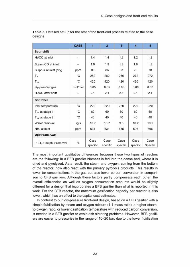
Table 5. Detailed set-up for the rest of the front-end process related to the case designs.
CASE 1 2 3 4 5
Sour shift
H2/CO at inlet – 1.4 1.4 1.3 1.2 1.2
Steam/CO at inlet – 1.9 1.9 1.8 1.8 1.8
Sulphur at inlet (dry) ppm 86 86 83 78 78
Tin °C 282 282 266 272 272
Tout °C 420 420 420 420 420
By-pass/syngas mol/mol 0.65 0.65 0.63 0.60 0.60
H2/CO after shift – 2.1 2.1 2.1 2.1 2.1
Scrubber
Inlet temperature °C 220 220 220 220 220
Tout at stage 1 °C 60 60 60 60 60
Tout at stage 2 °C 40 40 40 40 40
Water removal kg/s 10.7 10.7 9.5 10.2 10.2
NH3 at inlet ppm 631 631 635 606 606
Upstream AGR
CO2 + sulphur removal % Case
specific Case
specific Case
specific Case
specific Case
Specific The most important qualitative differences between these two types of reactors are the following: In a BFB gasifier biomass is fed into the dense bed, where it is dried and pyrolysed. As a result, the steam and oxygen, coming from the bottom of the reactor, now also react with the primary pyrolysis products. This results in lower tar concentrations in the gas but also lower carbon conversion in compari-son to CFB gasifiers. Although these factors partly compensate each other, the overall efficiencies as well as oxygen consumption amounts would be slightly different for a design that incorporates a BFB gasifier than what is reported in this work. For the BFB reactor, the maximum gasification capacity per reactor is also lower, which has an effect to the capital cost estimates.
In contrast to our low-pressure front-end design, based on a CFB gasifier with a simple fluidisation by steam and oxygen mixture (1:1 mass ratio), a higher steam-to-oxygen ratio, or lower gasification temperature with reduced carbon conversion, is needed in a BFB gasifier to avoid ash sintering problems. However, BFB gasifi-ers are easier to pressurise in the range of 10–20 bar, due to the lower fluidisation
4. Case designs and front-end results
34
velocities and easier recycle gas fluidisation arrangement, as demonstrated in the High Temperature Winkler gasifier operated in Finland in early 1990’s using peat as a feedstock.34
4.2 Front-end mass and energy balances
After having discussed the content of the five case designs, we analyse the ther-modynamic performance of these concepts based on our simulation results and using cold gas efficiency (5) as the metric.
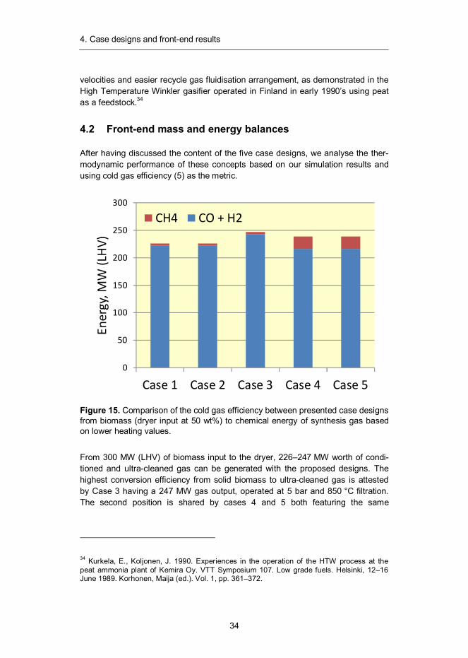
Figure 15. Comparison of the cold gas efficiency between presented case designs from biomass (dryer input at 50 wt%) to chemical energy of synthesis gas based on lower heating values.
From 300 MW (LHV) of biomass input to the dryer, 226–247 MW worth of condi-tioned and ultra-cleaned gas can be generated with the proposed designs. The highest conversion efficiency from solid biomass to ultra-cleaned gas is attested by Case 3 having a 247 MW gas output, operated at 5 bar and 850 °C filtration. The second position is shared by cases 4 and 5 both featuring the same
34 Kurkela, E., Koljonen, J. 1990. Experiences in the operation of the HTW process at the peat ammonia plant of Kemira Oy. VTT Symposium 107. Low grade fuels. Helsinki, 12–16 June 1989. Korhonen, Maija (ed.). Vol. 1, pp. 361–372.
0
50
100
150
200
250
300
Case 1 Case 2 Case 3 Case 4 Case 5
Ener
gy, M
W (L
HV)
CH4 CO + H2
4. Case designs and front-end results
35
22 bar/850 °C front-end leaving cases 1 and 2 (5 bar/550 °C front-ends) to the last place.
= , (5)
When we exclude the chemical energy of methane contained in the syngas we arrive to the amount of energy that is available for conversion in the synthesis. For cases employing 5 bar gasification and 550 °C filtration this amounts to 222 MW, which is increased to 243 MW as a result of higher filtration temperature. For 22 bar gasification with 850 °C filtration, the combined energy of CO and H2 is 216 MW, the lowest for all of the simulated front-end designs. As percentages these results are 74.1% (for Case 1 and Case 2), 81.1% (for Case 3) and 72.1% (for Case 4 and Case 5).
The above comparison reveals important features of the UCG process that per-colate through all of our subsequent analysis: the higher methane slip associated with higher gasification pressure significantly reduces the amount of energy that is eventually available for conversion into liquid fuel. In addition, large fraction of inerts in the make-up gas leads to larger recycle gas amounts in the conversion loop and thus to larger equipment volumes and higher costs. Whether the com-pression savings that result from the higher front-end pressure are enough to counter these adverse effects to performance will be examined later with the help of economic analysis.
5. Process economics
36
5. Process economics
5.1 Cost estimation methodology
The scale of production is expected to be an important factor in the overall eco-nomic performance of a BTL plant. The basic assumption is that the decrease in specific investment cost due to economies of scale offsets the increase in biomass transportation cost as the scale of the plant grows larger. However, the availability of biomass severely limits the maximum size of a BTL plant. In observance of this limitation, we have chosen to set the scale of our examined plants to 300 MW LHV of biomass input (at 50 wt% moisture). We expect this scale to be large enough to reach some of the benefits from economies of scale, while still be small enough to facilitate extensive heat integration with existing processes or district heating net-works. We expect the range of accuracy in the capital cost estimates to be ±30%, a value typical for factored estimates.35
All cost estimates are generated for a Nth plant design. We expect the first commercial scale installations to be more expensive, but do not try to estimate how much. The capacity of the CFB gasifier is set to 300 MW and syntheses are expected to process all the synthesis gas in one train.
The capital cost estimates for the examined plant designs were developed to the Total Overnight Capital (TOC) cost level, which includes equipment, installa-tion and indirect construction costs. 30% contingency factor has been assigned for the front-end equipment and synthesis islands, while 20% is used for other, com-mercially mature, components. For the use of financial analysis, the TOC was modified to account for interest during construction (5% of TOC) yielding a Total Capital Investment (TCI) for each of the examined plant designs.
35 Cran, J. 1981. Improved factored method gives better preliminary cost estimates, Chem Eng, April 6.
5. Process economics
37
5.2 Capital cost estimates
Table 6. Reference equipment capacities, scaling exponents and costs for auxiliary equipment and power island including balance of plant.
Ref.
Cost scaling parameter
Capacity Scaling
exponent
Installed cost in
2010 M€
AUXILIARY EQUIPMENT
Site preparation
Buildings VTT Biomass input, MWth 200 0.85 9.1
Oxygen production
ASU (stand alone) EL Oxygen output, t/h 76.60 0.5 47.8
Feedstock pretreatment
Feedstock handling CB Biomass input, MWth 157 0.31 5.3
Belt dryer CB Water removal, kg/s 0.427 0.50 1.7
POWER ISLAND
Heat recovery from GI VTT Duty, MWth 43.6 0.8 5.2
Auxiliary boiler + HRSG VTT Boiler input, MWth 80 0.65 26.3
Steam turbine +
condenser AH Power out, MWe 22.5 0.85 6.6
VTT = VTT in-house estimate EL = Larson et al. 2009. Footnote [36] CB = Carbona Inc, 2009. Footnote [29] AH = Andras Horvath, 2012. Footnote [37]
The reference equipment costs were assembled using literature sources, vendor quotes, discussions with industry experts and engineering judgement. Individual cost scaling exponents (k) were used to scale reference capital costs (Co) to ca-pacity that corresponds with simulation results (S) using following relation:
= , (6)
where So is the scale of reference equipment and C the cost of equipment at the size suggested by our simulation. All reference costs in our database have been escalated to correspond 2010 euros using Chemical Engineering’s Plant Cost index38 (CEPCI) to account for the inflation.
36 Larson, E.D., Jin, H., Celik, F.E. 2009. Large-scale gasification-based coproduction of fuels and electricity from switchgrass, Biofuels, Biorprod. Bioref. 3:174–194. 37 Horvath, A. 2012. Personal communication. 38 Chemical Engineering; Apr 2012; 119, 4; ABI/INFORM Complete pg. 84, www.che.com/pci
5. Process economics
38
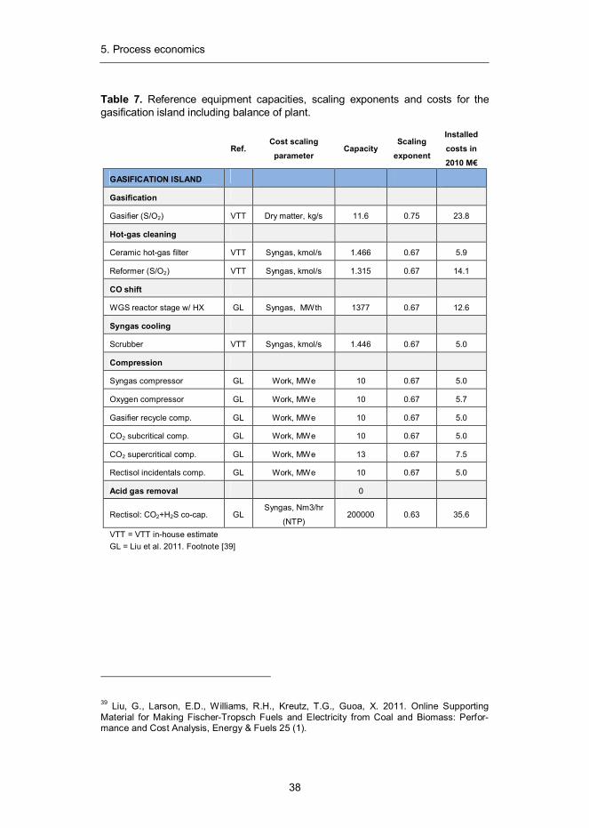
Table 7. Reference equipment capacities, scaling exponents and costs for the gasification island including balance of plant.
Ref.
Cost scaling parameter
Capacity Scaling
exponent
Installed costs in 2010 M€
GASIFICATION ISLAND
Gasification
Gasifier (S/O2) VTT Dry matter, kg/s 11.6 0.75 23.8
Hot-gas cleaning
Ceramic hot-gas filter VTT Syngas, kmol/s 1.466 0.67 5.9
Reformer (S/O2) VTT Syngas, kmol/s 1.315 0.67 14.1
CO shift
WGS reactor stage w/ HX GL Syngas, MWth 1377 0.67 12.6
Syngas cooling
Scrubber VTT Syngas, kmol/s 1.446 0.67 5.0
Compression
Syngas compressor GL Work, MWe 10 0.67 5.0
Oxygen compressor GL Work, MWe 10 0.67 5.7
Gasifier recycle comp. GL Work, MWe 10 0.67 5.0
CO2 subcritical comp. GL Work, MWe 10 0.67 5.0
CO2 supercritical comp. GL Work, MWe 13 0.67 7.5
Rectisol incidentals comp. GL Work, MWe 10 0.67 5.0
Acid gas removal
0
Rectisol: CO2+H2S co-cap. GL Syngas, Nm3/hr
(NTP) 200000 0.63 35.6
VTT = VTT in-house estimate GL = Liu et al. 2011. Footnote [39]
39 Liu, G., Larson, E.D., Williams, R.H., Kreutz, T.G., Guoa, X. 2011. Online Supporting Material for Making Fischer-Tropsch Fuels and Electricity from Coal and Biomass: Perfor-mance and Cost Analysis, Energy & Fuels 25 (1).
5. Process economics
39
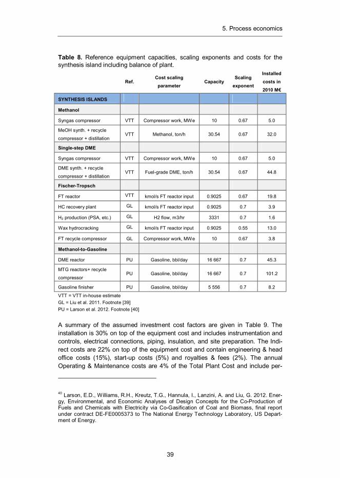
Table 8. Reference equipment capacities, scaling exponents and costs for the synthesis island including balance of plant.
Ref.
Cost scaling parameter
Capacity Scaling
exponent
Installed costs in 2010 M€
SYNTHESIS ISLANDS
Methanol
Syngas compressor VTT Compressor work, MWe 10 0.67 5.0
MeOH synth. + recycle
compressor + distillation VTT Methanol, ton/h 30.54 0.67 32.0
Single-step DME
Syngas compressor VTT Compressor work, MWe 10 0.67 5.0
DME synth. + recycle
compressor + distillation VTT Fuel-grade DME, ton/h 30.54 0.67 44.8
Fischer-Tropsch
FT reactor VTT kmol/s FT reactor input 0.9025 0.67 19.8
HC recovery plant GL kmol/s FT reactor input 0.9025 0.7 3.9
H2 production (PSA, etc.) GL H2 flow, m3/hr 3331 0.7 1.6
Wax hydrocracking GL kmol/s FT reactor input 0.9025 0.55 13.0
FT recycle compressor GL Compressor work, MWe 10 0.67 3.8
Methanol-to-Gasoline
DME reactor PU Gasoline, bbl/day 16 667 0.7 45.3
MTG reactors+ recycle
compressor PU Gasoline, bbl/day 16 667 0.7 101.2
Gasoline finisher PU Gasoline, bbl/day 5 556 0.7 8.2
VTT = VTT in-house estimate GL = Liu et al. 2011. Footnote [39] PU = Larson et al. 2012. Footnote [40] A summary of the assumed investment cost factors are given in Table 9. The installation is 30% on top of the equipment cost and includes instrumentation and controls, electrical connections, piping, insulation, and site preparation. The Indi-rect costs are 22% on top of the equipment cost and contain engineering & head office costs (15%), start-up costs (5%) and royalties & fees (2%). The annual Operating & Maintenance costs are 4% of the Total Plant Cost and include per-
40 Larson, E.D., Williams, R.H., Kreutz, T.G., Hannula, I., Lanzini, A. and Liu, G. 2012. Ener-gy, Environmental, and Economic Analyses of Design Concepts for the Co-Production of Fuels and Chemicals with Electricity via Co-Gasification of Coal and Biomass, final report under contract DE-FE0005373 to The National Energy Technology Laboratory, US Depart-ment of Energy.
5. Process economics
40
sonnel costs (0.5%), maintenance and insurances (2.5%) as well as catalysts & chemicals (1%).
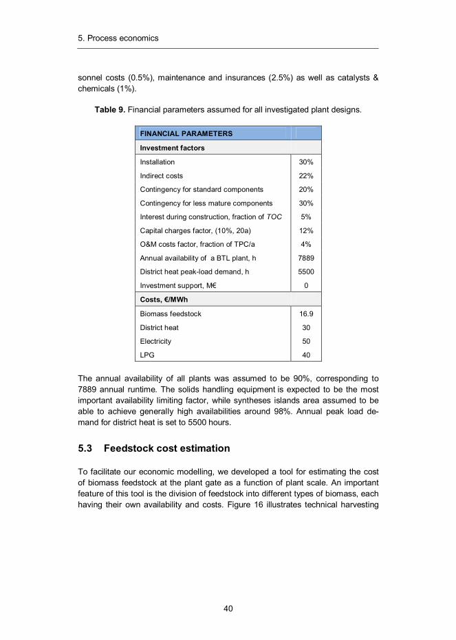
Table 9. Financial parameters assumed for all investigated plant designs.
FINANCIAL PARAMETERS
Investment factors
Installation 30%
Indirect costs 22%
Contingency for standard components 20%
Contingency for less mature components 30%
Interest during construction, fraction of TOC 5%
Capital charges factor, (10%, 20a) 12%
O&M costs factor, fraction of TPC/a 4%
Annual availability of a BTL plant, h 7889
District heat peak-load demand, h 5500
Investment support, M€ 0
Costs, €/MWh
Biomass feedstock 16.9
District heat 30
Electricity 50
LPG 40
The annual availability of all plants was assumed to be 90%, corresponding to 7889 annual runtime. The solids handling equipment is expected to be the most important availability limiting factor, while syntheses islands area assumed to be able to achieve generally high availabilities around 98%. Annual peak load de-mand for district heat is set to 5500 hours.
5.3 Feedstock cost estimation
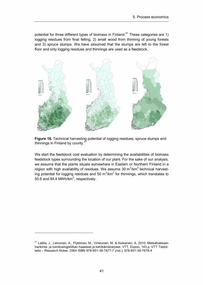
To facilitate our economic modelling, we developed a tool for estimating the cost of biomass feedstock at the plant gate as a function of plant scale. An important feature of this tool is the division of feedstock into different types of biomass, each having their own availability and costs. Figure 16 illustrates technical harvesting
5. Process economics
41
potential for three different types of biomass in Finland.41 These categories are 1) logging residues from final felling, 2) small wood from thinning of young forests and 3) spruce stumps. We have assumed that the stumps are left to the forest floor and only logging residues and thinnings are used as a feedstock.
Figure 16. Technical harvesting potential of logging residues, spruce stumps and thinnings in Finland by county.41
We start the feedstock cost evaluation by determining the availabilities of biomass feedstock types surrounding the location of our plant. For the sake of our analysis, we assume that the plants situate somewhere in Eastern or Northern Finland in a region with high availability of residues. We assume 30 m3/km2 technical harvest-ing potential for logging residues and 50 m3/km2 for thinnings, which translates to 50.6 and 84.4 MWh/km2, respectively.
41 Laitila, J., Leinonen, A., Flyktman, M., Virkkunen, M. & Asikainen, A. 2010. Metsähakkeen hankinta- ja toimituslogistiikan haasteet ja kehittämistarpeet. VTT, Espoo. 143 p. VTT Tiedot-teita – Research Notes: 2564 ISBN 978-951-38-7677-7 (nid.); 978-951-38-7678-4
5. Process economics
42
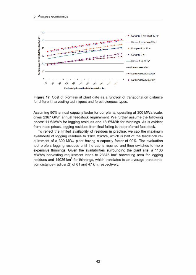
Figure 17. Cost of biomass at plant gate as a function of transportation distance for different harvesting techniques and forest biomass types.
Assuming 90% annual capacity factor for our plants, operating at 300 MWth scale, gives 2367 GWh annual feedstock requirement. We further assume the following prices: 11 €/MWh for logging residues and 18 €/MWh for thinnings. As is evident from these prices, logging residues from final felling is the preferred feedstock.
To reflect the limited availability of residues in practise, we cap the maximum availability of logging residues to 1183 MWh/a, which is half of the feedstock re-quirement of a 300 MWth plant having a capacity factor of 90%. The evaluation tool prefers logging residues until the cap is reached and then switches to more expensive thinnings. Given the availabilities surrounding the plant site, a 1183 MWh/a harvesting requirement leads to 23376 km2 harvesting area for logging residues and 14026 km2 for thinnings, which translates to an average transporta-tion distance (radius/ 2) of 61 and 47 km, respectively.
5. Process economics
43
Figure 18. Cost curves for biomass feedstock as a function of transportation dis-tance with different maximum amounts of logging residues assuming costs and availabilities discussed in the text.
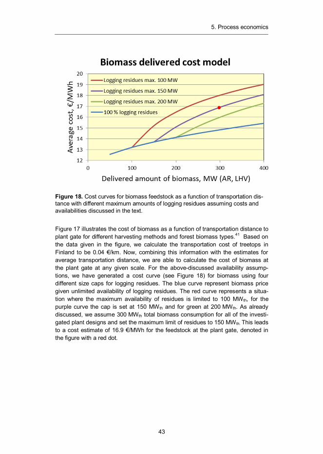
Figure 17 illustrates the cost of biomass as a function of transportation distance to plant gate for different harvesting methods and forest biomass types.41 Based on the data given in the figure, we calculate the transportation cost of treetops in Finland to be 0.04 €/km. Now, combining this information with the estimates for average transportation distance, we are able to calculate the cost of biomass at the plant gate at any given scale. For the above-discussed availability assump-tions, we have generated a cost curve (see Figure 18) for biomass using four different size caps for logging residues. The blue curve represent biomass price given unlimited availability of logging residues. The red curve represents a situa-tion where the maximum availability of residues is limited to 100 MWth, for the purple curve the cap is set at 150 MW th and for green at 200 MWth. As already discussed, we assume 300 MWth total biomass consumption for all of the investi-gated plant designs and set the maximum limit of residues to 150 MWth. This leads to a cost estimate of 16.9 €/MWh for the feedstock at the plant gate, denoted in the figure with a red dot.
6. Methanol synthesis design and results
44
6. Methanol synthesis design and results
Methanol, also known as methyl alcohol, is a well-known chemical with the formu-la CH3OH. It is the simplest of aliphatic alcohols and a light, volatile, colourless and flammable liquid at ambient conditions. It is miscible with water, alcohols and various organic solvents. Methanol (MeOH) is the largest product from synthesis gas after ammonia and can be utilised as chemical feedstock or as such to sup-plement liquid fuels. It can also be converted to acetic acid, formaldehyde, methyl methacrylate and methyl tertiary-butyl ether (MTBE) or used as a portal to hydro-carbon fuels through the conversion to dimethyl ether (DME) or gasoline (MTG). In 2011 the annual consumption of methanol amounted to 47 million tons, its largest consumer being formaldehyde industry followed by acetic acid industry.42
6.1 Introduction
The production of methanol from synthesis gas was first described by Patart43 and soon after produced by BASF chemists in Leuna, Germany in 1923.44 This be-came possible through the development of sulphur and chlorine resistant zinc oxide (ZnO-Cr2O3) catalyst, which benefitted from the engineering experience previously acquired through the development of ammonia synthesis technology.45 The main shortcoming of this process was the low activity of the catalyst, which required the use of relatively high reaction temperatures in the range of 300–400 °C. As a result, a high (about 350 bar) pressure was also needed to reach reasonable equilibrium conversions.46 Despite its drawbacks, high pressure meth-
42 Ott, J., Gronemann, V., Pontzen, F., Fiedler, E., Grossmann, G., Kerse-bohm, D., Weiss, G., Witte, C., Methanol. 2012. In Ullmann's Encyclope-dia of Industrial Chemistry, Wiley-VCH Verlag GmbH & Co. KgaA. 43 Patart, M., 1921, French patent, 540 343. 44 Tijm, P.J.A, Waller, G.J., Brown, D.M. 2001. Methanol technology devel-opments for the new millennium, Applied Catalysis A: General, Vol. 221(1–2), pp. 275–282, ISSN 0926-860X. 45 Appl, M., 1997, “Ammonia, Methanol, Hydrogen, Carbon Monoxide – Modern Production Technologies”, Nitrogen, ISBN 1-873387-26-1. 46 Mansfield, K. “ICI experience in methanol”. Nitrogen (221), 27 (May–Jun 1996).
6. Methanol synthesis design and results
45
anol synthesis was the principal industrial production route of methanol for 40 years. In 1960s workers at ICI pioneered an improved process using a more active and highly selective copper oxide catalyst, which became a practical option through the advent of virtually sulphur-free (H2S < 0.1 ppm) synthesis gas pro-duced by natural gas steam reformers. This low pressure methanol synthesis, operated at 250–280 °C and 60–80 bar has since become the exclusive produc-tion process for methanol at industrial scale with largest plants having a capacity of more than 500 metric tons per day (MTPD).47, 42
Methanol is synthesised by hydrogenation of carbon oxide over catalysts based on copper oxide, zinc oxide or chromium oxide. All commercially available modern catalyst systems are based on Cu-ZnO-Al2O3 or Cr2O3 with different additives and promoters. These catalysts allow the production of methanol with over 99.9% selectivity, with higher alcohols, ethers, esters, hydrocarbons and ketones as primary byproducts. In addition to water-gas shift reaction (1), methanol synthesis can be described with the following reactions48
+ 2 = , = 90.7 kJ/mol, (7)
+ 3 = + , = 40.9 kJ/mol. (8)
The kinetics and mechanisms of methanol synthesis have been discussed since the beginning of methanol research. An enduring question has been whether the formation of methanol proceeds primarily via CO or CO2 hydrogenation; some authors have reported sharp maximum of reaction rate for CO2 contents in the range of 2–5%, while others report constant increase with increasing CO2 con-tent.42 According to Hansen [48], there is an array of evidence favouring the CO2 route to methanol and only few proponents exists anymore who believe that meth-anol is formed from CO in any substantial quantities, at least with industrial cata-lysts and conditions. As both methanol reactions are exothermic and accompanied by net decrease in molar volume, the equilibrium is favoured by high pressure and low temperature. However, the copper-based catalyst is not active at temperatures much lower than 220 °C and a compromise between reaction kinetics and equilib-rium considerations is required.49 The methanol synthesis is characterised by ratio (H2 - CO2) / (CO + CO2), where H2, CO and CO2 represent their respective con-centrations in the make-up gas, continuously fed to the synthesis loop. This ratio, often referred to as the module M, should equal 2.03 for an ideal make-up gas
47 Lange, J., Methanol synthesis: a short review of technology improvements, Catalysis Today, Volume 64, Issues 1–2, 1 January 2001, Pages 3–8, ISSN 0920-5861. 48 Hansen, J.B., Methanol Synthesis, in: Ertl, G., Knözinger, H., Weitkamp, J.: Handbook of Heterogeneous Catalysis, Vol. 4, VCH, Weinheim (1997), p. 1856. 49 “Converter options for methanol synthesis”. Nitrogen (210), 36–44 (Jul–Aug 1994).
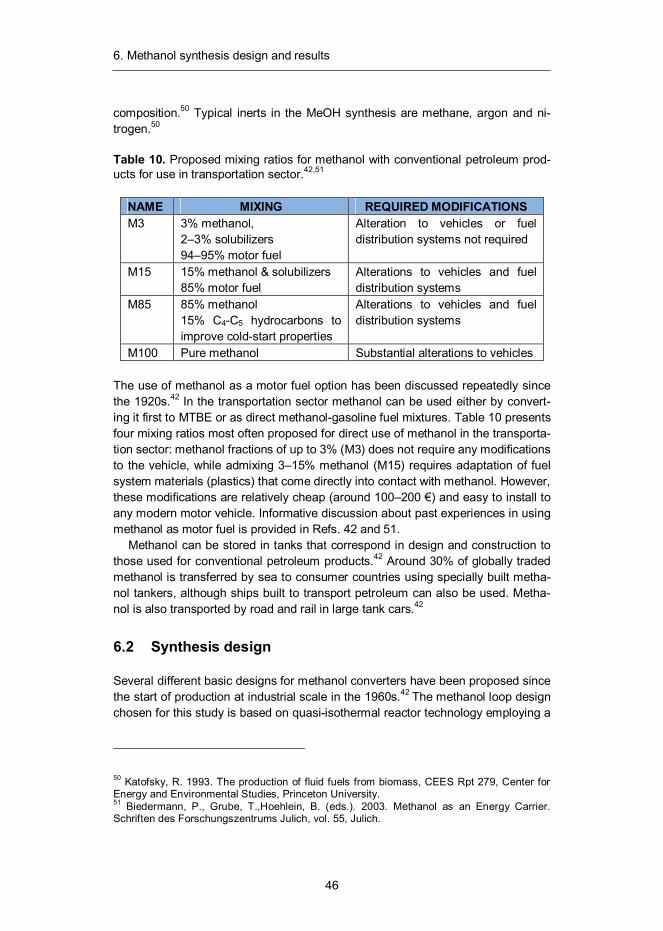
6. Methanol synthesis design and results
46
composition.50 Typical inerts in the MeOH synthesis are methane, argon and ni-trogen.50
Table 10. Proposed mixing ratios for methanol with conventional petroleum prod-ucts for use in transportation sector.42,51
NAME MIXING REQUIRED MODIFICATIONS M3 3% methanol,
2–3% solubilizers 94–95% motor fuel
Alteration to vehicles or fuel distribution systems not required
M15 15% methanol & solubilizers 85% motor fuel
Alterations to vehicles and fuel distribution systems
M85 85% methanol 15% C4-C5 hydrocarbons to improve cold-start properties
Alterations to vehicles and fuel distribution systems
M100 Pure methanol Substantial alterations to vehicles
The use of methanol as a motor fuel option has been discussed repeatedly since the 1920s.42 In the transportation sector methanol can be used either by convert-ing it first to MTBE or as direct methanol-gasoline fuel mixtures. Table 10 presents four mixing ratios most often proposed for direct use of methanol in the transporta-tion sector: methanol fractions of up to 3% (M3) does not require any modifications to the vehicle, while admixing 3–15% methanol (M15) requires adaptation of fuel system materials (plastics) that come directly into contact with methanol. However, these modifications are relatively cheap (around 100–200 €) and easy to install to any modern motor vehicle. Informative discussion about past experiences in using methanol as motor fuel is provided in Refs. 42 and 51.
Methanol can be stored in tanks that correspond in design and construction to those used for conventional petroleum products.42 Around 30% of globally traded methanol is transferred by sea to consumer countries using specially built metha-nol tankers, although ships built to transport petroleum can also be used. Metha-nol is also transported by road and rail in large tank cars.42
6.2 Synthesis design
Several different basic designs for methanol converters have been proposed since the start of production at industrial scale in the 1960s.42 The methanol loop design chosen for this study is based on quasi-isothermal reactor technology employing a
50 Katofsky, R. 1993. The production of fluid fuels from biomass, CEES Rpt 279, Center for Energy and Environmental Studies, Princeton University. 51 Biedermann, P., Grube, T.,Hoehlein, B. (eds.). 2003. Methanol as an Energy Carrier. Schriften des Forschungszentrums Julich, vol. 55, Julich.
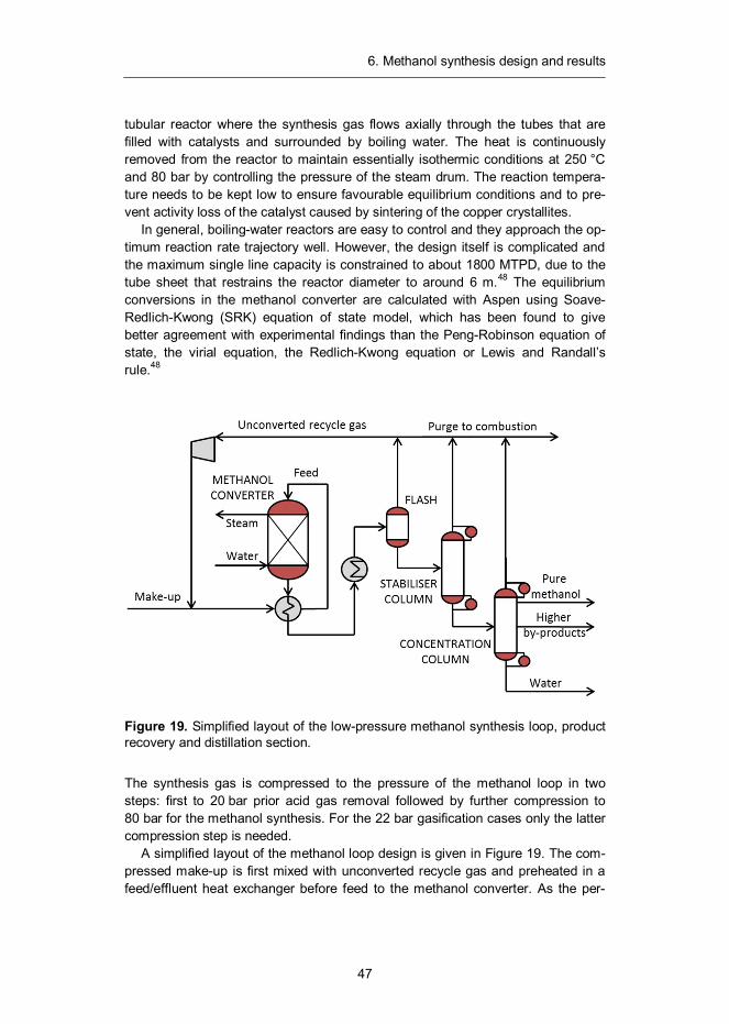
6. Methanol synthesis design and results
47
tubular reactor where the synthesis gas flows axially through the tubes that are filled with catalysts and surrounded by boiling water. The heat is continuously removed from the reactor to maintain essentially isothermic conditions at 250 °C and 80 bar by controlling the pressure of the steam drum. The reaction tempera-ture needs to be kept low to ensure favourable equilibrium conditions and to pre-vent activity loss of the catalyst caused by sintering of the copper crystallites.
In general, boiling-water reactors are easy to control and they approach the op-timum reaction rate trajectory well. However, the design itself is complicated and the maximum single line capacity is constrained to about 1800 MTPD, due to the tube sheet that restrains the reactor diameter to around 6 m.48 The equilibrium conversions in the methanol converter are calculated with Aspen using Soave-Redlich-Kwong (SRK) equation of state model, which has been found to give better agreement with experimental findings than the Peng-Robinson equation of state, the virial equation, the Redlich-Kwong equation or Lewis and Randall’s rule.48
Figure 19. Simplified layout of the low-pressure methanol synthesis loop, product recovery and distillation section.
The synthesis gas is compressed to the pressure of the methanol loop in two steps: first to 20 bar prior acid gas removal followed by further compression to 80 bar for the methanol synthesis. For the 22 bar gasification cases only the latter compression step is needed.
A simplified layout of the methanol loop design is given in Figure 19. The com-pressed make-up is first mixed with unconverted recycle gas and preheated in a feed/effluent heat exchanger before feed to the methanol converter. As the per-
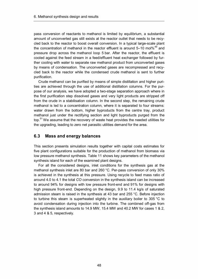
6. Methanol synthesis design and results
48
pass conversion of reactants to methanol is limited by equilibrium, a substantial amount of unconverted gas still exists at the reactor outlet that needs to be recy-cled back to the reactor to boost overall conversion. In a typical large-scale plant the concentration of methanol in the reactor effluent is around 5–10 mol%49 and pressure drop across the methanol loop 5 bar. After the reactor, the effluent is cooled against the feed stream in a feed/effluent heat exchanger followed by fur-ther cooling with water to separate raw methanol product from unconverted gases by means of condensation. The unconverted gases are recompressed and recy-cled back to the reactor while the condensed crude methanol is sent to further purification.
Crude methanol can be purified by means of simple distillation and higher puri-ties are achieved through the use of additional distillation columns. For the pur-pose of our analysis, we have adopted a two-stage separation approach where in the first purification step dissolved gases and very light products are stripped off from the crude in a stabilisation column. In the second step, the remaining crude methanol is led to a concentration column, where it is separated to four streams: water drawn from the bottom, higher byproducts from the centre tray, product methanol just under the rectifying section and light byproducts purged from the top.51 We assume that the recovery of waste heat provides the needed utilities for the upgrading, leading to zero net parasitic utilities demand for the area.
6.3 Mass and energy balances
This section presents simulation results together with capital costs estimates for five plant configurations suitable for the production of methanol from biomass via low pressure methanol synthesis. Table 11 shows key parameters of the methanol synthesis island for each of the examined plant designs.
For all the considered designs, inlet conditions for the synthesis gas at the methanol synthesis inlet are 80 bar and 260 °C. Per-pass conversion of only 30% is achieved in the synthesis at this pressure. Using recycle to feed mass ratio of around 4.0 to 4.1 the total CO conversion in the synthesis island can be increased to around 94% for designs with low pressure front-end and 91% for designs with high pressure front-end. Depending on the design, 9.9 to 11.4 kg/s of saturated admission steam is raised in the synthesis at 43 bar and 255 °C. Before injection to turbine this steam is superheated slightly in the auxiliary boiler to 305 °C to avoid condensation during injection into the turbine. The combined off-gas from the synthesis island amounts to 14.9 MW, 15.4 MW and 40.2 MW for cases 1 & 2, 3 and 4 & 5, respectively.
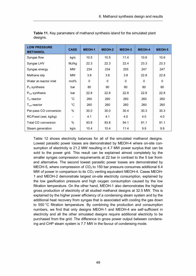
6. Methanol synthesis design and results
49
Table 11. Key parameters of methanol synthesis island for the simulated plant designs.
LOW PRESSURE METHANOL
CASE MEOH-1 MEOH-2 MEOH-3 MEOH-4 MEOH-5
Syngas flow kg/s 10.5 10.5 11.4 10.6 10.6
Syngas LHV MJ/kg 22.3 22.3 22.4 23.3 23.3
Syngas energy MW 234 234 255 247 247
Methane slip MW 3.8 3.8 3.8 22.8 22.8
Water at reactor inlet mol% 0 0 0 0 0
Pin synthesis bar 80 80 80 80 80
Pout synthesis bar 22.8 22.8 22.8 22.8 22.8
Tin reactor °C 260 260 260 260 260
Tout reactor °C 260 260 260 260 260
Per-pass CO conversion % 30.0 30.0 30.4 30.3 30.3
RC/Feed (wet, kg/kg) - 4.1 4.1 4.0 4.0 4.0
Total CO conversion % 93.8 93.8 94.1 91.1 91.1
Steam generation kg/s 10.4 10.4 11.4 9.9 9.9
Table 12 shows electricity balances for all of the simulated methanol designs. Lowest parasitic power losses are demonstrated by MEOH-4 where on-site con-sumption of electricity is 21.2 MW resulting in 4.7 MW power surplus that can be sold to the power grid. This result can be explained almost completely by the smaller syngas compression requirements at 22 bar in contrast to the 5 bar front-end alternative. The second lowest parasitic power losses are demonstrated by MEOH-5, where compression of CO2 to 150 bar pressure consumes additional 6.4 MW of power in comparison to its CO2 venting equivalent MEOH-4. Cases MEOH-1 and MEOH-2 demonstrate largest on-site electricity consumption, explained by the low gasification pressure and high oxygen consumption caused by the low filtration temperature. On the other hand, MEOH-1 also demonstrates the highest gross production of electricity of all studied methanol designs at 32.5 MW. This is explained by the higher power efficiency of a condensing steam system and by the additional heat recovery from syngas that is associated with cooling the gas down to 550 °C filtration temperature. By combining the production and consumption numbers, we find that only designs MEOH-1 and MEOH-4 are self-sufficient in electricity and all the other simulated designs require additional electricity to be purchased from the grid. The difference in gross power output between condens-ing and CHP steam system is 7.7 MW in the favour of condensing mode.
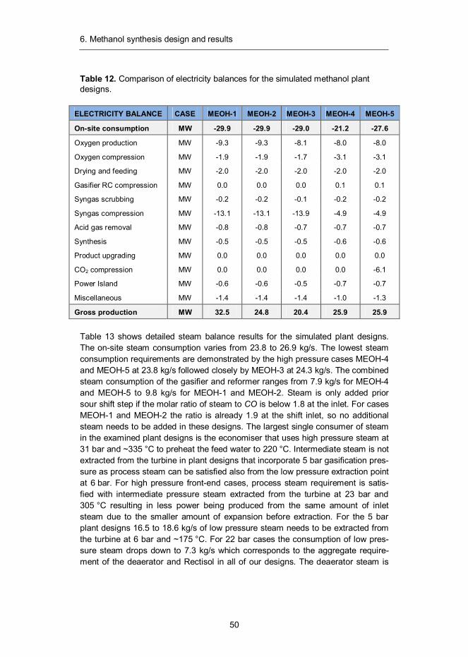
6. Methanol synthesis design and results
50
Table 12. Comparison of electricity balances for the simulated methanol plant designs.
ELECTRICITY BALANCE CASE MEOH-1 MEOH-2 MEOH-3 MEOH-4 MEOH-5
On-site consumption MW -29.9 -29.9 -29.0 -21.2 -27.6
Oxygen production MW -9.3 -9.3 -8.1 -8.0 -8.0
Oxygen compression MW -1.9 -1.9 -1.7 -3.1 -3.1
Drying and feeding MW -2.0 -2.0 -2.0 -2.0 -2.0
Gasifier RC compression MW 0.0 0.0 0.0 0.1 0.1
Syngas scrubbing MW -0.2 -0.2 -0.1 -0.2 -0.2
Syngas compression MW -13.1 -13.1 -13.9 -4.9 -4.9
Acid gas removal MW -0.8 -0.8 -0.7 -0.7 -0.7
Synthesis MW -0.5 -0.5 -0.5 -0.6 -0.6
Product upgrading MW 0.0 0.0 0.0 0.0 0.0
CO2 compression MW 0.0 0.0 0.0 0.0 -6.1
Power Island MW -0.6 -0.6 -0.5 -0.7 -0.7
Miscellaneous MW -1.4 -1.4 -1.4 -1.0 -1.3
Gross production MW 32.5 24.8 20.4 25.9 25.9
Table 13 shows detailed steam balance results for the simulated plant designs. The on-site steam consumption varies from 23.8 to 26.9 kg/s. The lowest steam consumption requirements are demonstrated by the high pressure cases MEOH-4 and MEOH-5 at 23.8 kg/s followed closely by MEOH-3 at 24.3 kg/s. The combined steam consumption of the gasifier and reformer ranges from 7.9 kg/s for MEOH-4 and MEOH-5 to 9.8 kg/s for MEOH-1 and MEOH-2. Steam is only added prior sour shift step if the molar ratio of steam to CO is below 1.8 at the inlet. For cases MEOH-1 and MEOH-2 the ratio is already 1.9 at the shift inlet, so no additional steam needs to be added in these designs. The largest single consumer of steam in the examined plant designs is the economiser that uses high pressure steam at 31 bar and ~335 °C to preheat the feed water to 220 °C. Intermediate steam is not extracted from the turbine in plant designs that incorporate 5 bar gasification pres-sure as process steam can be satisfied also from the low pressure extraction point at 6 bar. For high pressure front-end cases, process steam requirement is satis-fied with intermediate pressure steam extracted from the turbine at 23 bar and 305 °C resulting in less power being produced from the same amount of inlet steam due to the smaller amount of expansion before extraction. For the 5 bar plant designs 16.5 to 18.6 kg/s of low pressure steam needs to be extracted from the turbine at 6 bar and ~175 °C. For 22 bar cases the consumption of low pres-sure steam drops down to 7.3 kg/s which corresponds to the aggregate require-ment of the deaerator and Rectisol in all of our designs. The deaerator steam is
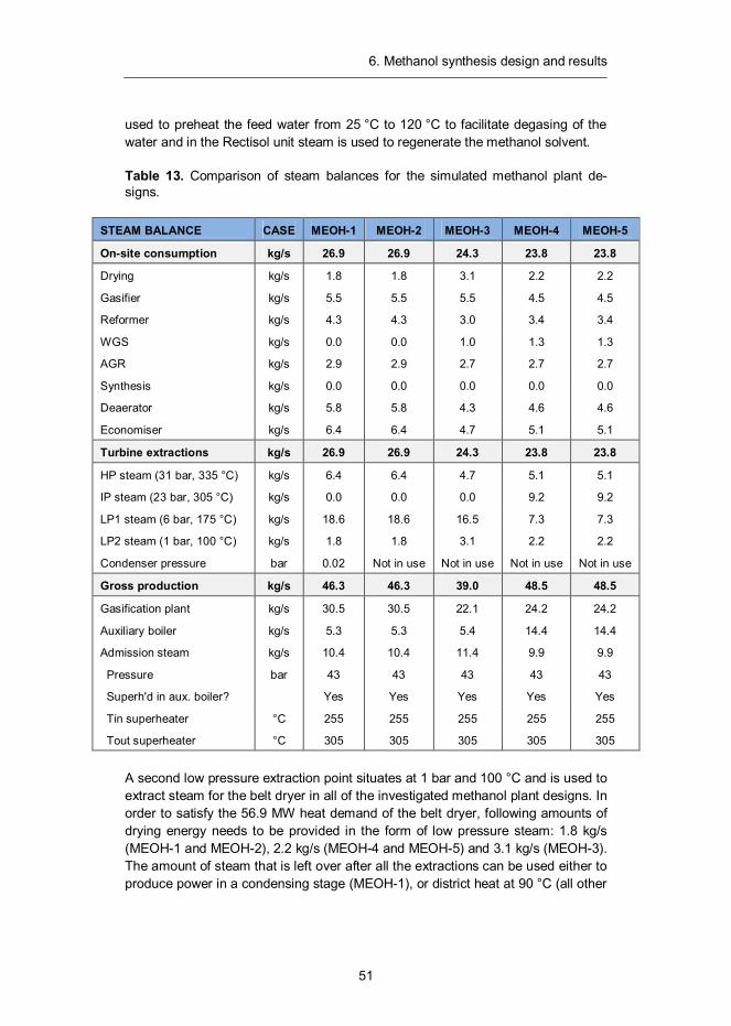
6. Methanol synthesis design and results
51
used to preheat the feed water from 25 °C to 120 °C to facilitate degasing of the water and in the Rectisol unit steam is used to regenerate the methanol solvent.
Table 13. Comparison of steam balances for the simulated methanol plant de-signs.
STEAM BALANCE CASE MEOH-1 MEOH-2 MEOH-3 MEOH-4 MEOH-5
On-site consumption kg/s 26.9 26.9 24.3 23.8 23.8
Drying kg/s 1.8 1.8 3.1 2.2 2.2
Gasifier kg/s 5.5 5.5 5.5 4.5 4.5
Reformer kg/s 4.3 4.3 3.0 3.4 3.4
WGS kg/s 0.0 0.0 1.0 1.3 1.3
AGR kg/s 2.9 2.9 2.7 2.7 2.7
Synthesis kg/s 0.0 0.0 0.0 0.0 0.0
Deaerator kg/s 5.8 5.8 4.3 4.6 4.6
Economiser kg/s 6.4 6.4 4.7 5.1 5.1
Turbine extractions kg/s 26.9 26.9 24.3 23.8 23.8
HP steam (31 bar, 335 °C) kg/s 6.4 6.4 4.7 5.1 5.1
IP steam (23 bar, 305 °C) kg/s 0.0 0.0 0.0 9.2 9.2
LP1 steam (6 bar, 175 °C) kg/s 18.6 18.6 16.5 7.3 7.3
LP2 steam (1 bar, 100 °C) kg/s 1.8 1.8 3.1 2.2 2.2
Condenser pressure bar 0.02 Not in use Not in use Not in use Not in use
Gross production kg/s 46.3 46.3 39.0 48.5 48.5
Gasification plant kg/s 30.5 30.5 22.1 24.2 24.2
Auxiliary boiler kg/s 5.3 5.3 5.4 14.4 14.4
Admission steam kg/s 10.4 10.4 11.4 9.9 9.9
Pressure bar 43 43 43 43 43
Superh'd in aux. boiler?
Yes Yes Yes Yes Yes
Tin superheater °C 255 255 255 255 255
Tout superheater °C 305 305 305 305 305
A second low pressure extraction point situates at 1 bar and 100 °C and is used to extract steam for the belt dryer in all of the investigated methanol plant designs. In order to satisfy the 56.9 MW heat demand of the belt dryer, following amounts of drying energy needs to be provided in the form of low pressure steam: 1.8 kg/s (MEOH-1 and MEOH-2), 2.2 kg/s (MEOH-4 and MEOH-5) and 3.1 kg/s (MEOH-3). The amount of steam that is left over after all the extractions can be used either to produce power in a condensing stage (MEOH-1), or district heat at 90 °C (all other
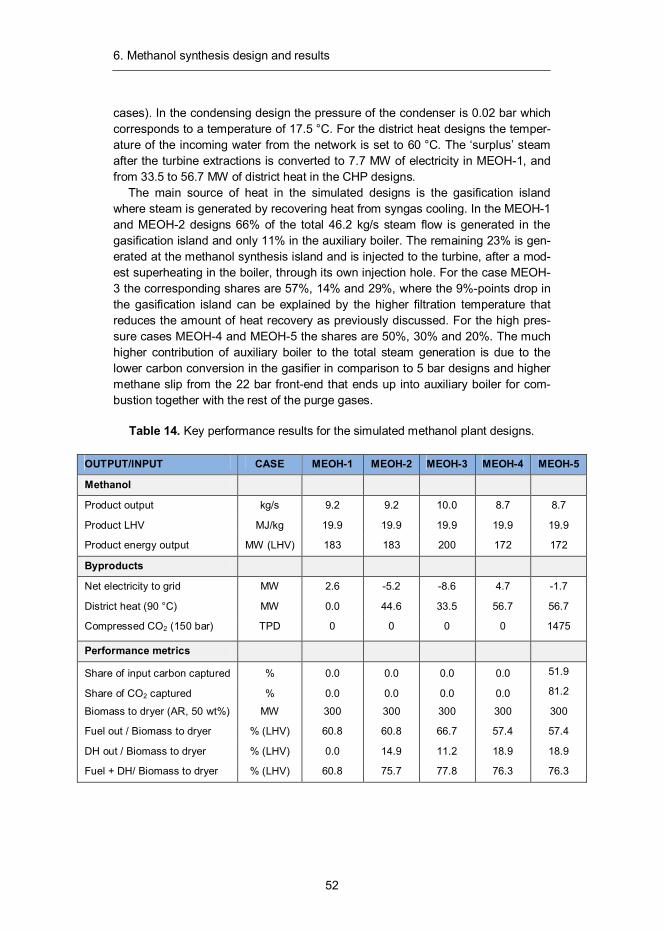
6. Methanol synthesis design and results
52
cases). In the condensing design the pressure of the condenser is 0.02 bar which corresponds to a temperature of 17.5 °C. For the district heat designs the temper-ature of the incoming water from the network is set to 60 °C. The ‘surplus’ steam after the turbine extractions is converted to 7.7 MW of electricity in MEOH-1, and from 33.5 to 56.7 MW of district heat in the CHP designs.
The main source of heat in the simulated designs is the gasification island where steam is generated by recovering heat from syngas cooling. In the MEOH-1 and MEOH-2 designs 66% of the total 46.2 kg/s steam flow is generated in the gasification island and only 11% in the auxiliary boiler. The remaining 23% is gen-erated at the methanol synthesis island and is injected to the turbine, after a mod-est superheating in the boiler, through its own injection hole. For the case MEOH-3 the corresponding shares are 57%, 14% and 29%, where the 9%-points drop in the gasification island can be explained by the higher filtration temperature that reduces the amount of heat recovery as previously discussed. For the high pres-sure cases MEOH-4 and MEOH-5 the shares are 50%, 30% and 20%. The much higher contribution of auxiliary boiler to the total steam generation is due to the lower carbon conversion in the gasifier in comparison to 5 bar designs and higher methane slip from the 22 bar front-end that ends up into auxiliary boiler for com-bustion together with the rest of the purge gases.
Table 14. Key performance results for the simulated methanol plant designs.
OUTPUT/INPUT CASE MEOH-1 MEOH-2 MEOH-3 MEOH-4 MEOH-5
Methanol
Product output kg/s 9.2 9.2 10.0 8.7 8.7
Product LHV MJ/kg 19.9 19.9 19.9 19.9 19.9
Product energy output MW (LHV) 183 183 200 172 172
Byproducts
Net electricity to grid MW 2.6 -5.2 -8.6 4.7 -1.7
District heat (90 °C) MW 0.0 44.6 33.5 56.7 56.7
Compressed CO2 (150 bar) TPD 0 0 0 0 1475
Performance metrics
Share of input carbon captured % 0.0 0.0 0.0 0.0 51.9
Share of CO2 captured % 0.0 0.0 0.0 0.0 81.2
Biomass to dryer (AR, 50 wt%) MW 300 300 300 300 300
Fuel out / Biomass to dryer % (LHV) 60.8 60.8 66.7 57.4 57.4
DH out / Biomass to dryer % (LHV) 0.0 14.9 11.2 18.9 18.9
Fuel + DH/ Biomass to dryer % (LHV) 60.8 75.7 77.8 76.3 76.3
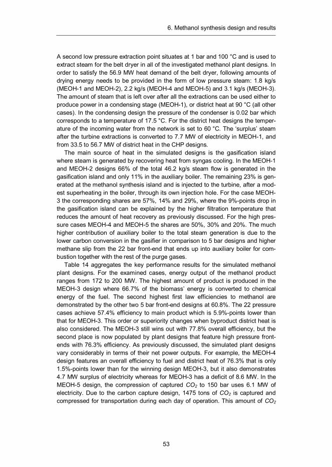
6. Methanol synthesis design and results
53
A second low pressure extraction point situates at 1 bar and 100 °C and is used to extract steam for the belt dryer in all of the investigated methanol plant designs. In order to satisfy the 56.9 MW heat demand of the belt dryer, following amounts of drying energy needs to be provided in the form of low pressure steam: 1.8 kg/s (MEOH-1 and MEOH-2), 2.2 kg/s (MEOH-4 and MEOH-5) and 3.1 kg/s (MEOH-3). The amount of steam that is left over after all the extractions can be used either to produce power in a condensing stage (MEOH-1), or district heat at 90 °C (all other cases). In the condensing design the pressure of the condenser is 0.02 bar which corresponds to a temperature of 17.5 °C. For the district heat designs the temper-ature of the incoming water from the network is set to 60 °C. The ‘surplus’ steam after the turbine extractions is converted to 7.7 MW of electricity in MEOH-1, and from 33.5 to 56.7 MW of district heat in the CHP designs.
The main source of heat in the simulated designs is the gasification island where steam is generated by recovering heat from syngas cooling. In the MEOH-1 and MEOH-2 designs 66% of the total 46.2 kg/s steam flow is generated in the gasification island and only 11% in the auxiliary boiler. The remaining 23% is gen-erated at the methanol synthesis island and is injected to the turbine, after a mod-est superheating in the boiler, through its own injection hole. For the case MEOH-3 the corresponding shares are 57%, 14% and 29%, where the 9%-points drop in the gasification island can be explained by the higher filtration temperature that reduces the amount of heat recovery as previously discussed. For the high pres-sure cases MEOH-4 and MEOH-5 the shares are 50%, 30% and 20%. The much higher contribution of auxiliary boiler to the total steam generation is due to the lower carbon conversion in the gasifier in comparison to 5 bar designs and higher methane slip from the 22 bar front-end that ends up into auxiliary boiler for com-bustion together with the rest of the purge gases.
Table 14 aggregates the key performance results for the simulated methanol plant designs. For the examined cases, energy output of the methanol product ranges from 172 to 200 MW. The highest amount of product is produced in the MEOH-3 design where 66.7% of the biomass’ energy is converted to chemical energy of the fuel. The second highest first law efficiencies to methanol are demonstrated by the other two 5 bar front-end designs at 60.8%. The 22 pressure cases achieve 57.4% efficiency to main product which is 5.9%-points lower than that for MEOH-3. This order or superiority changes when byproduct district heat is also considered. The MEOH-3 still wins out with 77.8% overall efficiency, but the second place is now populated by plant designs that feature high pressure front-ends with 76.3% efficiency. As previously discussed, the simulated plant designs vary considerably in terms of their net power outputs. For example, the MEOH-4 design features an overall efficiency to fuel and district heat of 76.3% that is only 1.5%-points lower than for the winning design MEOH-3, but it also demonstrates 4.7 MW surplus of electricity whereas for MEOH-3 has a deficit of 8.6 MW. In the MEOH-5 design, the compression of captured CO2 to 150 bar uses 6.1 MW of electricity. Due to the carbon capture design, 1475 tons of CO2 is captured and compressed for transportation during each day of operation. This amount of CO2
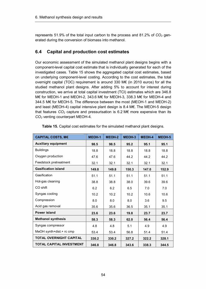
6. Methanol synthesis design and results
54
represents 51.9% of the total input carbon to the process and 81.2% of CO2 gen-erated during the conversion of biomass into methanol.
6.4 Capital and production cost estimates
Our economic assessment of the simulated methanol plant designs begins with a component-level capital cost estimate that is individually generated for each of the investigated cases. Table 15 shows the aggregated capital cost estimates, based on underlying component-level costing. According to the cost estimates, the total overnight capital (TOC) requirement is around 330 M€ (in 2010 euros) for all the studied methanol plant designs. After adding 5% to account for interest during construction, we arrive at total capital investment (TCI) estimates which are 346.8 M€ for MEOH-1 and MEOH-2, 343.6 M€ for MEOH-3, 338.3 M€ for MEOH-4 and 344.5 M€ for MEOH-5. The difference between the most (MEOH-1 and MEOH-2) and least (MEOH-4) capital intensive plant design is 8.4 M€. The MEOH-5 design that features CO2 capture and pressurisation is 6.2 M€ more expensive than its CO2 venting counterpart MEOH-4.
Table 15. Capital cost estimates for the simulated methanol plant designs.
CAPITAL COSTS, M€ MEOH-1 MEOH-2 MEOH-3 MEOH-4 MEOH-5
Auxiliary equipment 98.5 98.5 95.2 95.1 95.1
Buildings 18.8 18.8 18.8 18.8 18.8
Oxygen production 47.6 47.6 44.2 44.2 44.2
Feedstock pretreatment 32.1 32.1 32.1 32.1 32.1
Gasification island 149.8 149.8 150.3 147.0 152.9
Gasification 51.1 51.1 51.1 51.1 51.1
Hot-gas cleaning 38.8 38.8 38.0 39.6 39.6
CO shift 6.2 6.2 6.5 7.0 7.0
Syngas cooling 10.2 10.2 10.2 10.6 10.6
Compression 8.0 8.0 8.0 3.6 9.5
Acid gas removal 35.6 35.6 36.5 35.1 35.1
Power island 23.6 23.6 19.8 23.7 23.7
Methanol synthesis 58.3 58.3 62.0 56.4 56.4
Syngas compressor 4.8 4.8 5.1 4.9 4.9
MeOH synth+dist.+ rc cmp 53.4 53.4 56.8 51.4 51.4
TOTAL OVERNIGHT CAPITAL 330.2 330.2 327.2 322.2 328.1
TOTAL CAPITAL INVESTMENT 346.8 346.8 343.6 338.3 344.5
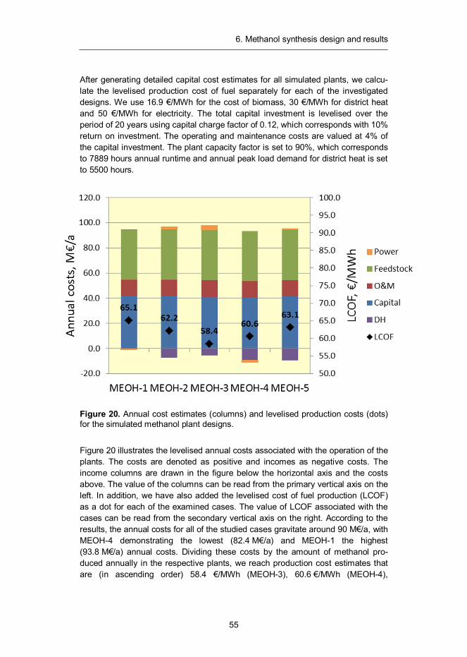
6. Methanol synthesis design and results
55
After generating detailed capital cost estimates for all simulated plants, we calcu-late the levelised production cost of fuel separately for each of the investigated designs. We use 16.9 €/MWh for the cost of biomass, 30 €/MWh for district heat and 50 €/MWh for electricity. The total capital investment is levelised over the period of 20 years using capital charge factor of 0.12, which corresponds with 10% return on investment. The operating and maintenance costs are valued at 4% of the capital investment. The plant capacity factor is set to 90%, which corresponds to 7889 hours annual runtime and annual peak load demand for district heat is set to 5500 hours.
Figure 20. Annual cost estimates (columns) and levelised production costs (dots) for the simulated methanol plant designs.
Figure 20 illustrates the levelised annual costs associated with the operation of the plants. The costs are denoted as positive and incomes as negative costs. The income columns are drawn in the figure below the horizontal axis and the costs above. The value of the columns can be read from the primary vertical axis on the left. In addition, we have also added the levelised cost of fuel production (LCOF) as a dot for each of the examined cases. The value of LCOF associated with the cases can be read from the secondary vertical axis on the right. According to the results, the annual costs for all of the studied cases gravitate around 90 M€/a, with MEOH-4 demonstrating the lowest (82.4 M€/a) and MEOH-1 the highest (93.8 M€/a) annual costs. Dividing these costs by the amount of methanol pro-duced annually in the respective plants, we reach production cost estimates that are (in ascending order) 58.4 €/MWh (MEOH-3), 60.6 €/MWh (MEOH-4),

6. Methanol synthesis design and results
56
62.2 €/MWh (MEOH-2), 63.1 €/MWh (MEOH-5) and 65.1 €/MWh (MEOH-1). The difference between the lowest and highest annual costs in the simulated designs is 11.5 M€ and the difference between LCOFs is 6.7 €/MWh. The change from condensing mode to CHP mode lowers the LCOF by 3.0 €/MWh and increasing filtration temperature from 550 to 850 °C lowers the LCOF further down by 3.7 €/MWh. The increase of gasification pressure from 5 to 22 bar (assuming previously discussed changes in the performance of the front-end process) in-creases LCOF by 2.1 €/MWh and compressing the separated CO2 stream ready for transportation increases LCOF by 2.6 €/MWh
7. Dimethyl ether synthesis design and results
57
7. Dimethyl ether synthesis design and results
Dimethyl ether (DME) is an organic compound with the formula CH3OCH3. It is the simplest of ethers and exists as a colourless gas at room temperature.52 The phys-ical properties of DME resemble those of liquefied petroleum gas (propane and butane) and it decomposes to water and carbon dioxide within a short time.53,54 DME is widely used as a propellant for various aerosol products, but is less famil-iar as a fuel option. With no carbon-carbon bonds, it burns without soot with a visible blue flame and has a high cetane number, making it an excellent substitute for conventional diesel and LPG. However, the need for compression to store it as liquid can be considered as a drawback in comparison to other synthetic transpor-tation fuels.
7.1 Introduction
Production of dimethyl ether involves dewatering of methanol over a gamma-alumina or aluminosilicate dehydration catalyst by the following reaction
2 = + 23,4 kJ/mol. (9)
Commercial production of DME involves a two-step process where methanol is first produced and then dehydrated in a separate step. However, an emerging option also exists where methanol and dehydration catalysts are mixed into the same reactor so that reactions (7) and (9) can proceed simultaneously making it possible to produce DME directly from syngas in a single step.
52 Dimethyl ether. 2012. In Wikipedia, The Free Encyclopedia. Retrieved 11:04, July 26, 2012, from tinyurl.com/cnl25t5 53 Semelsberger, T., Borup, R. and Greene, H. 2006. Dimethyl ether (DME) as an alternative fuel, Journal of Power Sources, Vol. 156(2), pp. 497–511. 54 Navqi, S. 2002. Dimethyl ether as alternative fuel, Report No. 245, SRI Consulting, Menlo Park, CA.
7. Dimethyl ether synthesis design and results
58
Modern catalysts are able to convert syngas to methanol close to the extent predicted by chemical equilibrium. In a single-step DME production, some of the formed methanol is continuously reacted away along with reaction (9), which al-lows the methanol reaction to advance further. Methanol catalysts also promote water-gas shift reaction (1), which introduces yet another synergistic effect: the water formed in the dehydration of methanol drives water-gas shift and the result-ing H2 boosts methanol production. The entire single-step DME synthesis can thus be described with the following reaction
3 + 3 = + 246 kJ/mol. (10)
The one-step DME synthesis can be carried out either in a fixed-bed or a slurry-phase reactor. The latter design has been more actively researched due to better reaction heat management capabilities. A practical temperature range for reactor operation that balances requirements of kinetics, catalyst activity and equilibrium is 250–280 °C whereas a practical pressure range falls between 15–150 kg/cm2 (15–147 bar).54
7.2 Synthesis design
The DME synthesis simulated in this study is based on Haldor Topsøe’s fixed-bed reactor design55, while the recovery and distillation section for the preparation of fuel-grade dimethyl ether follows closely information disclosed in Ref. 56. The term fuel-grade refers to a final purification design were some methanol and water are left to the final product. It has been shown57 that relatively large amounts (< 20 wt%) of these diluents can be tolerated without exceeding emissions regula-tions in compression ignition engines. Three to four reactors with cooling between stages is suggested for large-scale DME synthesis, but for a smaller process, single reactor with multi-layered catalyst bed with cooling between layers may be used. The equilibrium conversions in the single-step DME reactor are calculated with Aspen using Soave-Redlich-Kwong (SRK) equation of state model.
The synthesis gas is compressed to reactor pressure in two steps: first to 20 bar prior acid gas removal step and then further to 60 bar prior inlet to the DME synthesis. For the 22 bar gasification cases only the latter compression step is necessary. The make-up gas is first mixed with unconverted gases from the recy-cle loop and preheated to 240 °C in heat exchange with the hot reactor effluent.
55 Voss, B., Joensen, F. and Hansen, J. 1996. Preparation of fuel grade di-methyl ether. Granted patent, EP 0871602 B1. 56 Haugaard, J. and Voss, B. 2000. Process for the synthesis of a metha-nol/dimethyl ether mixture from synthesis gas. Granted patent, US 6191175. 57 Fleisch, T., McCarthy, C, Basu, A., Udovich, C., Charbonneau, P., Slodowske, Mikkelsen, S.E., McCandless, D. 1995. A New Clean Diesel Technology, Int. Congr. & Expos., Detroit, Michigan, Feb. 27–March 2, 1995.
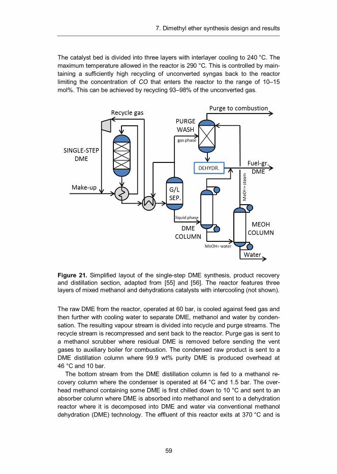
7. Dimethyl ether synthesis design and results
59
The catalyst bed is divided into three layers with interlayer cooling to 240 °C. The maximum temperature allowed in the reactor is 290 °C. This is controlled by main-taining a sufficiently high recycling of unconverted syngas back to the reactor limiting the concentration of CO that enters the reactor to the range of 10–15 mol%. This can be achieved by recycling 93–98% of the unconverted gas.
Figure 21. Simplified layout of the single-step DME synthesis, product recovery and distillation section, adapted from [55] and [56]. The reactor features three layers of mixed methanol and dehydrations catalysts with intercooling (not shown).
The raw DME from the reactor, operated at 60 bar, is cooled against feed gas and then further with cooling water to separate DME, methanol and water by conden-sation. The resulting vapour stream is divided into recycle and purge streams. The recycle stream is recompressed and sent back to the reactor. Purge gas is sent to a methanol scrubber where residual DME is removed before sending the vent gases to auxiliary boiler for combustion. The condensed raw product is sent to a DME distillation column where 99.9 wt% purity DME is produced overhead at 46 °C and 10 bar.
The bottom stream from the DME distillation column is fed to a methanol re-covery column where the condenser is operated at 64 °C and 1.5 bar. The over-head methanol containing some DME is first chilled down to 10 °C and sent to an absorber column where DME is absorbed into methanol and sent to a dehydration reactor where it is decomposed into DME and water via conventional methanol dehydration (DME) technology. The effluent of this reactor exits at 370 °C and is
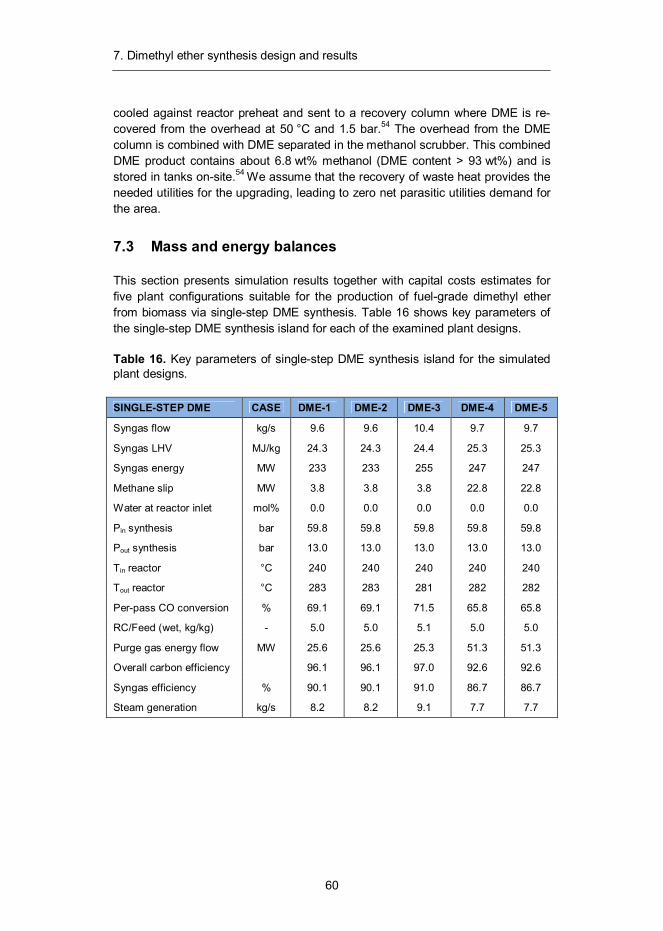
7. Dimethyl ether synthesis design and results
60
cooled against reactor preheat and sent to a recovery column where DME is re-covered from the overhead at 50 °C and 1.5 bar.54 The overhead from the DME column is combined with DME separated in the methanol scrubber. This combined DME product contains about 6.8 wt% methanol (DME content > 93 wt%) and is stored in tanks on-site.54 We assume that the recovery of waste heat provides the needed utilities for the upgrading, leading to zero net parasitic utilities demand for the area.
7.3 Mass and energy balances
This section presents simulation results together with capital costs estimates for five plant configurations suitable for the production of fuel-grade dimethyl ether from biomass via single-step DME synthesis. Table 16 shows key parameters of the single-step DME synthesis island for each of the examined plant designs.
Table 16. Key parameters of single-step DME synthesis island for the simulated plant designs.
SINGLE-STEP DME CASE DME-1 DME-2 DME-3 DME-4 DME-5
Syngas flow kg/s 9.6 9.6 10.4 9.7 9.7
Syngas LHV MJ/kg 24.3 24.3 24.4 25.3 25.3
Syngas energy MW 233 233 255 247 247
Methane slip MW 3.8 3.8 3.8 22.8 22.8
Water at reactor inlet mol% 0.0 0.0 0.0 0.0 0.0
Pin synthesis bar 59.8 59.8 59.8 59.8 59.8
Pout synthesis bar 13.0 13.0 13.0 13.0 13.0
Tin reactor °C 240 240 240 240 240
Tout reactor °C 283 283 281 282 282
Per-pass CO conversion % 69.1 69.1 71.5 65.8 65.8
RC/Feed (wet, kg/kg) - 5.0 5.0 5.1 5.0 5.0
Purge gas energy flow MW 25.6 25.6 25.3 51.3 51.3
Overall carbon efficiency 96.1 96.1 97.0 92.6 92.6
Syngas efficiency % 90.1 90.1 91.0 86.7 86.7
Steam generation kg/s 8.2 8.2 9.1 7.7 7.7
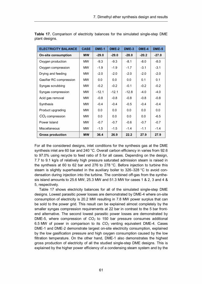
7. Dimethyl ether synthesis design and results
61
Table 17. Comparison of electricity balances for the simulated single-step DME plant designs.
ELECTRICITY BALANCE CASE DME-1 DME-2 DME-3 DME-4 DME-5
On-site consumption MW -29.0 -29.0 -28.0 -20.2 -27.0
Oxygen production MW -9.3 -9.3 -8.1 -8.0 -8.0
Oxygen compression MW -1.9 -1.9 -1.7 -3.1 -3.1
Drying and feeding MW -2.0 -2.0 -2.0 -2.0 -2.0
Gasifier RC compression MW 0.0 0.0 0.0 0.1 0.1
Syngas scrubbing MW -0.2 -0.2 -0.1 -0.2 -0.2
Syngas compression MW -12.1 -12.1 -12.8 -4.0 -4.0
Acid gas removal MW -0.8 -0.8 -0.8 -0.8 -0.8
Synthesis MW -0.4 -0.4 -0.5 -0.4 -0.4
Product upgrading MW 0.0 0.0 0.0 0.0 0.0
CO2 compression MW 0.0 0.0 0.0 0.0 -6.5
Power Island MW -0.7 -0.7 -0.6 -0.7 -0.7
Miscellaneous MW -1.5 -1.5 -1.4 -1.1 -1.4
Gross production MW 36.4 26.9 22.2 27.9 27.9
For all the considered designs, inlet conditions for the synthesis gas at the DME synthesis inlet are 60 bar and 240 °C. Overall carbon efficiency in varies from 92.6 to 97.0% using recycle to feed ratio of 5 for all cases. Depending on the design, 7.7 to 9.1 kg/s of relatively high pressure saturated admission steam is raised in the synthesis at 60 to 62 bar and 276 to 278 °C. Before injection to turbine this steam is slightly superheated in the auxiliary boiler to 326–328 °C to avoid con-densation during injection into the turbine. The combined off-gas from the synthe-sis island amounts to 25.6 MW, 25.3 MW and 51.3 MW for cases 1 & 2, 3 and 4 & 5, respectively.
Table 17 shows electricity balances for all of the simulated single-step DME designs. Lowest parasitic power losses are demonstrated by DME-4 where on-site consumption of electricity is 20.2 MW resulting in 7.8 MW power surplus that can be sold to the power grid. This result can be explained almost completely by the smaller syngas compression requirements at 22 bar in contrast to the 5 bar front-end alternative. The second lowest parasitic power losses are demonstrated by DME-5, where compression of CO2 to 150 bar pressure consumes additional 6.5 MW of power in comparison to its CO2 venting equivalent DME-4. Cases DME-1 and DME-2 demonstrate largest on-site electricity consumption, explained by the low gasification pressure and high oxygen consumption caused by the low filtration temperature. On the other hand, DME-1 also demonstrates the highest gross production of electricity of all the studied single-step DME designs. This is explained by the higher power efficiency of a condensing steam system and by the
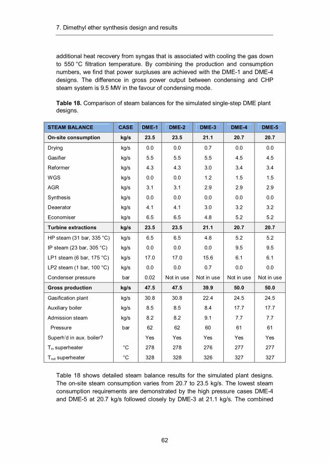
7. Dimethyl ether synthesis design and results
62
additional heat recovery from syngas that is associated with cooling the gas down to 550 °C filtration temperature. By combining the production and consumption numbers, we find that power surpluses are achieved with the DME-1 and DME-4 designs. The difference in gross power output between condensing and CHP steam system is 9.5 MW in the favour of condensing mode.
Table 18. Comparison of steam balances for the simulated single-step DME plant designs.
STEAM BALANCE CASE DME-1 DME-2 DME-3 DME-4 DME-5
On-site consumption kg/s 23.5 23.5 21.1 20.7 20.7
Drying kg/s 0.0 0.0 0.7 0.0 0.0
Gasifier kg/s 5.5 5.5 5.5 4.5 4.5
Reformer kg/s 4.3 4.3 3.0 3.4 3.4
WGS kg/s 0.0 0.0 1.2 1.5 1.5
AGR kg/s 3.1 3.1 2.9 2.9 2.9
Synthesis kg/s 0.0 0.0 0.0 0.0 0.0
Deaerator kg/s 4.1 4.1 3.0 3.2 3.2
Economiser kg/s 6.5 6.5 4.8 5.2 5.2
Turbine extractions kg/s 23.5 23.5 21.1 20.7 20.7
HP steam (31 bar, 335 °C) kg/s 6.5 6.5 4.8 5.2 5.2
IP steam (23 bar, 305 °C) kg/s 0.0 0.0 0.0 9.5 9.5
LP1 steam (6 bar, 175 °C) kg/s 17.0 17.0 15.6 6.1 6.1
LP2 steam (1 bar, 100 °C) kg/s 0.0 0.0 0.7 0.0 0.0
Condenser pressure bar 0.02 Not in use Not in use Not in use Not in use
Gross production kg/s 47.5 47.5 39.9 50.0 50.0
Gasification plant kg/s 30.8 30.8 22.4 24.5 24.5
Auxiliary boiler kg/s 8.5 8.5 8.4 17.7 17.7
Admission steam kg/s 8.2 8.2 9.1 7.7 7.7
Pressure bar 62 62 60 61 61
Superh’d in aux. boiler? Yes Yes Yes Yes Yes
Tin superheater °C 278 278 276 277 277
Tout superheater °C 328 328 326 327 327
Table 18 shows detailed steam balance results for the simulated plant designs. The on-site steam consumption varies from 20.7 to 23.5 kg/s. The lowest steam consumption requirements are demonstrated by the high pressure cases DME-4 and DME-5 at 20.7 kg/s followed closely by DME-3 at 21.1 kg/s. The combined
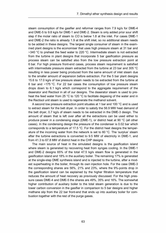
7. Dimethyl ether synthesis design and results
63
steam consumption of the gasifier and reformer ranges from 7.9 kg/s for DME-4 and DME-5 to 9.8 kg/s for DME-1 and DME-2. Steam is only added prior sour shift step if the molar ratio of steam to CO is below 1.8 at the inlet. For cases DME-1 and DME-2 the ratio is already 1.9 at the shift inlet, so no additional steam needs to be added in these designs. The largest single consumer of steam in the exam-ined plant designs is the economiser that uses high pressure steam at 31 bar and ~340 °C to preheat the feed water to 220 °C. Intermediate steam is not extracted from the turbine in plant designs that incorporate 5 bar gasification pressure as process steam can be satisfied also from the low pressure extraction point at 6 bar. For high pressure front-end cases, process steam requirement is satisfied with intermediate pressure steam extracted from the turbine at 23 bar and 305 °C resulting in less power being produced from the same amount of inlet steam due to the smaller amount of expansion before extraction. For the 5 bar plant designs 15.6 to 17.0 kg/s of low pressure steam needs to be extracted from the turbine at 6 bar and ~175 °C. For 22 bar cases the consumption of low pressure steam drops down to 6.1 kg/s which correspond to the aggregate requirement of the deaerator and Rectisol in all of our designs. The deaerator steam is used to pre-heat the feed water from 25 °C to 120 °C to facilitate degasing of the water and in the Rectisol unit steam is used to regenerate the methanol solvent.
A second low pressure extraction point situates at 1 bar and 100 °C and is used to extract steam for the belt dryer. In order to satisfy the 56.9 MW heat demand of the belt dryer, 0.7 kg/s of steam needs to be extracted in the DME-3 design. The amount of steam that is left over after all the extractions can be used either to produce power in a condensing stage (DME-1), or district heat at 90 °C (all other cases). In the condensing design the pressure of the condenser is 0.02 bar which corresponds to a temperature of 17.5 °C. For the district heat designs the temper-ature of the incoming water from the network is set to 60 °C. The ‘surplus’ steam after the turbine extractions is converted to 9.5 MW of electricity in DME-1, and from 41.3 to 67.8 MW of district heat in the CHP designs
The main source of heat in the simulated designs is the gasification island where steam is generated by recovering heat from syngas cooling. In the DME-1 and DME-2 designs 65% of the total 47.5 kg/s steam flow is generated in the gasification island and 18% in the auxiliary boiler. The remaining 17% is generated at the single-step DME synthesis island and is injected to the turbine, after a mod-est superheating in the boiler, through its own injection hole. For the case DME-3 the corresponding shares are 56%, 21% and 23%, where the 9%-points drop in the gasification island can be explained by the higher filtration temperature that reduces the amount of heat recovery as previously discussed. For the high pres-sure cases DME-4 and DME-5 the shares are 49%, 35% and 16%. The somewhat higher contribution of auxiliary boiler to the total steam generation is due to the lower carbon conversion in the gasifier in comparison to 5 bar designs and higher methane slip from the 22 bar front-end that ends up into auxiliary boiler for com-bustion together with the rest of the purge gases.
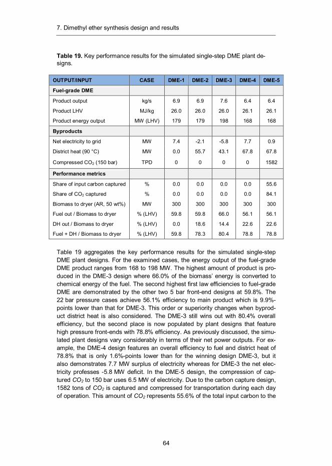
7. Dimethyl ether synthesis design and results
64
Table 19. Key performance results for the simulated single-step DME plant de-signs.
OUTPUT/INPUT CASE DME-1 DME-2 DME-3 DME-4 DME-5
Fuel-grade DME Product output kg/s 6.9 6.9 7.6 6.4 6.4
Product LHV MJ/kg 26.0 26.0 26.0 26.1 26.1
Product energy output MW (LHV) 179 179 198 168 168
Byproducts Net electricity to grid MW 7.4 -2.1 -5.8 7.7 0.9
District heat (90 °C) MW 0.0 55.7 43.1 67.8 67.8
Compressed CO2 (150 bar) TPD 0 0 0 0 1582
Performance metrics Share of input carbon captured % 0.0 0.0 0.0 0.0 55.6
Share of CO2 captured % 0.0 0.0 0.0 0.0 84.1
Biomass to dryer (AR, 50 wt%) MW 300 300 300 300 300
Fuel out / Biomass to dryer % (LHV) 59.8 59.8 66.0 56.1 56.1
DH out / Biomass to dryer % (LHV) 0.0 18.6 14.4 22.6 22.6
Fuel + DH / Biomass to dryer % (LHV) 59.8 78.3 80.4 78.8 78.8
Table 19 aggregates the key performance results for the simulated single-step DME plant designs. For the examined cases, the energy output of the fuel-grade DME product ranges from 168 to 198 MW. The highest amount of product is pro-duced in the DME-3 design where 66.0% of the biomass’ energy is converted to chemical energy of the fuel. The second highest first law efficiencies to fuel-grade DME are demonstrated by the other two 5 bar front-end designs at 59.8%. The 22 bar pressure cases achieve 56.1% efficiency to main product which is 9.9%-points lower than that for DME-3. This order or superiority changes when byprod-uct district heat is also considered. The DME-3 still wins out with 80.4% overall efficiency, but the second place is now populated by plant designs that feature high pressure front-ends with 78.8% efficiency. As previously discussed, the simu-lated plant designs vary considerably in terms of their net power outputs. For ex-ample, the DME-4 design features an overall efficiency to fuel and district heat of 78.8% that is only 1.6%-points lower than for the winning design DME-3, but it also demonstrates 7.7 MW surplus of electricity whereas for DME-3 the net elec-tricity professes -5.8 MW deficit. In the DME-5 design, the compression of cap-tured CO2 to 150 bar uses 6.5 MW of electricity. Due to the carbon capture design, 1582 tons of CO2 is captured and compressed for transportation during each day of operation. This amount of CO2 represents 55.6% of the total input carbon to the
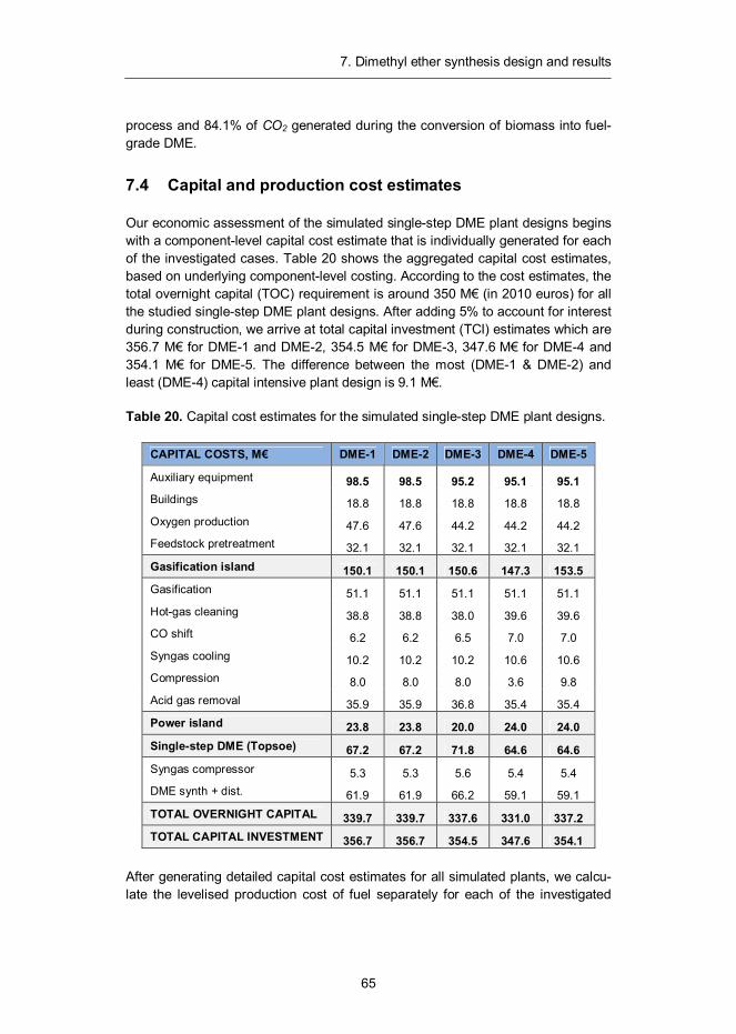
7. Dimethyl ether synthesis design and results
65
process and 84.1% of CO2 generated during the conversion of biomass into fuel-grade DME.
7.4 Capital and production cost estimates
Our economic assessment of the simulated single-step DME plant designs begins with a component-level capital cost estimate that is individually generated for each of the investigated cases. Table 20 shows the aggregated capital cost estimates, based on underlying component-level costing. According to the cost estimates, the total overnight capital (TOC) requirement is around 350 M€ (in 2010 euros) for all the studied single-step DME plant designs. After adding 5% to account for interest during construction, we arrive at total capital investment (TCI) estimates which are 356.7 M€ for DME-1 and DME-2, 354.5 M€ for DME-3, 347.6 M€ for DME-4 and 354.1 M€ for DME-5. The difference between the most (DME-1 & DME-2) and least (DME-4) capital intensive plant design is 9.1 M€.
Table 20. Capital cost estimates for the simulated single-step DME plant designs.
CAPITAL COSTS, M€ DME-1 DME-2 DME-3 DME-4 DME-5
Auxiliary equipment 98.5 98.5 95.2 95.1 95.1 Buildings 18.8 18.8 18.8 18.8 18.8 Oxygen production 47.6 47.6 44.2 44.2 44.2 Feedstock pretreatment 32.1 32.1 32.1 32.1 32.1 Gasification island 150.1 150.1 150.6 147.3 153.5 Gasification 51.1 51.1 51.1 51.1 51.1 Hot-gas cleaning 38.8 38.8 38.0 39.6 39.6 CO shift 6.2 6.2 6.5 7.0 7.0 Syngas cooling 10.2 10.2 10.2 10.6 10.6 Compression 8.0 8.0 8.0 3.6 9.8 Acid gas removal 35.9 35.9 36.8 35.4 35.4 Power island 23.8 23.8 20.0 24.0 24.0 Single-step DME (Topsoe) 67.2 67.2 71.8 64.6 64.6 Syngas compressor 5.3 5.3 5.6 5.4 5.4 DME synth + dist. 61.9 61.9 66.2 59.1 59.1 TOTAL OVERNIGHT CAPITAL 339.7 339.7 337.6 331.0 337.2 TOTAL CAPITAL INVESTMENT 356.7 356.7 354.5 347.6 354.1
After generating detailed capital cost estimates for all simulated plants, we calcu-late the levelised production cost of fuel separately for each of the investigated
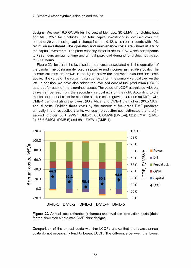
7. Dimethyl ether synthesis design and results
66
designs. We use 16.9 €/MWh for the cost of biomass, 30 €/MWh for district heat and 50 €/MWh for electricity. The total capital investment is levelised over the period of 20 years using capital charge factor of 0.12, which corresponds with 10% return on investment. The operating and maintenance costs are valued at 4% of the capital investment. The plant capacity factor is set to 90%, which corresponds to 7889 hours annual runtime and annual peak load demand for district heat is set to 5500 hours.
Figure 22 illustrates the levelised annual costs associated with the operation of the plants. The costs are denoted as positive and incomes as negative costs. The income columns are drawn in the figure below the horizontal axis and the costs above. The value of the columns can be read from the primary vertical axis on the left. In addition, we have also added the levelised cost of fuel production (LCOF) as a dot for each of the examined cases. The value of LCOF associated with the cases can be read from the secondary vertical axis on the right. According to the results, the annual costs for all of the studied cases gravitate around 90 M€/a, with DME-4 demonstrating the lowest (80.7 M€/a) and DME-1 the highest (93.5 M€/a) annual costs. Dividing these costs by the amount of fuel-grade DME produced annually in the respective plants, we reach production cost estimates that are (in ascending order) 58.4 €/MWh (DME-3), 60.8 €/MWh (DME-4), 62.2 €/MWh (DME-2), 63.6 €/MWh (DME-5) and 66.1 €/MWh (DME-1).
Figure 22. Annual cost estimates (columns) and levelised production costs (dots) for the simulated single-step DME plant designs.
Comparison of the annual costs with the LCOFs shows that the lowest annual costs do not necessarily lead to lowest LCOF. The difference between the lowest
7. Dimethyl ether synthesis design and results
67
and highest annual costs in the simulated designs is 12.7 M€ and the difference between LCOFs is 7.7 €/MWh. The change from condensing mode to CHP mode lowers the LCOF by 3.8 €/MWh and increasing filtration temperature from 550 to 850 °C lowers the LCOF further down by 3.8 €/MWh. The increase of gasification pressure from 5 to 22 bar (assuming previously discussed changes in the perfor-mance of the front-end process) actually increases LCOF by 2.4 €/MWh and com-pressing the separated CO2 stream ready for transportation increases LCOF by 2.8 €/MWh
8. Fischer-Tropsch synthesis design and results
68
8. Fischer-Tropsch synthesis design and results
Technologies that enable the production of liquid fuels from solid or gaseous hy-drocarbons have existed for almost a century. The most widely used method for indirect liquefaction involves gasification of coal into synthesis gas, which is sub-sequently cleaned and converted to liquid using Fischer-Tropsch process. As the byproduct CO2 from these liquefaction processes equals in net GHG emissions about double of those from petroleum fuels,58 seeking ways to reduce the envi-ronmental footprint of the process has become an area of active research. Fre-quently proposed methods for decarbonation include addition of carbon capture and storage, co-gasification of coal and biomass or dedicated biomass gasifica-tion.59,60,61,62,
8.1 Introduction
Conversion of synthesis gas to aliphatic hydrocarbons over metal catalysts was first discovered in the early 1920’s by Franz Fischer and Hans Tropsch at the Kaiser-Wilhelm-Institut für Kohlenforschung in Mülheim, Germany. Fischer and Tropsch showed that hydrogenation of CO over iron, cobalt and nickel catalysts result in a product mixture of linear hydrocarbons at 180–250 °C and atmospheric
58 Kreutz, T.G., Larson, E.D., Williams, R.H., Liu, G. 2008. Fischer-Tropsch Fuels from Coal and Biomass. In Proceedings of the 25th Annual Interna-tional Pittsburgh Coal Conference, Pittsburgh, PA. 59 Guangjian, L., Eric, D. Larson, R.H., Williams, T.G. Kreutz, and Guo, X. 2011. Making Fischer Tropsch Fuels and Electricity from Coal and Bio-mass: Performance and Cost Analysis Energy & Fuels 25 (1), pp. 415-437. 60 Van Bibber, L., Shuster, E., Haslbeck, J., Rutkowski, M., Olsen, S., Kra-mer, S. 2007. Baseline Technical and Economic Assessment of a Com-mercial Scale Fischer-Tropsch Liquids Facility; DOE/NETL-2007/1260; National Energy Technology Laboratory: Pittsburgh. 61 Hamelinck, C., Faaij, A., den Uil, H., Boerrigter, H. 2004. Production of FT transportation fuels from biomass; technical options, process analysis and optimisation, and development potential, Energy, Vol. 29(11), pp. 1743–1771, ISSN 0360-5442. 62 McKeough, P. and Kurkela, E. 2008. Process evaluations and design studies in the UCG project 2004–2007, VTT Research notes 2434, Espoo Finland. tinyurl.com/bre4cdx
8. Fischer-Tropsch synthesis design and results
69
pressure.63,64 This process, called the FT synthesis, has since experienced period-ical industrial deployment, first in the 1940’s to provide liquid hydrocarbon fuels for the German war effort and later for South Africa during the apartheid induced trade sanctions. Present interest to FT has been fuelled by increased discovery of gas fields at remote locations where no market for natural gas exists. The possibil-ity to convert these “stranded” reserves to transportable FT liquids has led to the deployment of gigantic gas-to-liquid plants in Malaysia (Bintulu) and Qatar (Pearl GTL).
The Fischer-Tropsch process is based on the following reaction65
(2 + 1) + ( ) + , (11)
where n is an integer and CnH(2n+2) represents the product that consists mainly of paraffinic hydrocarbons of variable chain length. Process conditions for the syn-thesis are usually chosen to maximise the formation of higher molecular weight liquid fuels which are higher value products.66 The raw product from the FT syn-thesis is called syncrude, which is recovered from the reactor outlet and refined to produce marketable hydrocarbon liquids such as high cetane diesel fuel.
The FT process can also be used to produce gasoline, but the overall complexi-ty of this application makes it less attractive than the diesel fuel option, where high linearity and low aromatic content of the syncrude are desirable features during refining.78 The fuel products from the FT process are of very high quality, showing excellent combustion properties (smoke point and cetane number), cold-flow characteristics and very low particle emissions. Meeting all relevant specifications, makes FT fuels excellent blending components for upgrading refinery fractions that would otherwise only be used in fuel oil.70 For example, the final diesel prod-uct can have a cetane number of 70, and as the market usually requires a cetane number of only 45, FT diesel can either be used in areas with very tight specifica-tions, or as blending stock for upgrading lower quality diesel.78
The characteristics of the FT synthesis product depends on the catalyst, pro-cess conditions and reactor design, ranging from methane to high molecular weight paraffins and olefins.67 A small amount of low molecular weight oxygenates such as alcohols and organic acids are also formed.66 The product distribution obeys a relationship called the ASF-distribution (Anderson-Schulz-Flory), which can be described fairly accurately by a simple statistical model (See Figure 23)
63 Fischer, F., Tropsch, H. Uber die Herstellung synthetischer ¨olgemische (Synthol) durch Aufbau aus Kohlenoxyd und Wasserstoff, Brennst. Chem. 4 (1923), pp. 276–285. 64 Fischer, F., Tropsch, H., German Patent 484337 1925. 65 Sie, S.T., Krishna, R. 1999. Fundamentals and selection of advanced Fischer–Tropsch reactors, Applied Catalysis A: General, Vol. 186(1–2), pp. 55–70. 66 Fischer-Tropsch (FT) Synthesis, NETL website, accessed July 23rd 2012, http://tinyurl.com/bvoumbw 67 de Klerk, A. 2011. Fischer-Tropsch refining, Wiley-VCH, 642 p. ISBN 9783527326051.
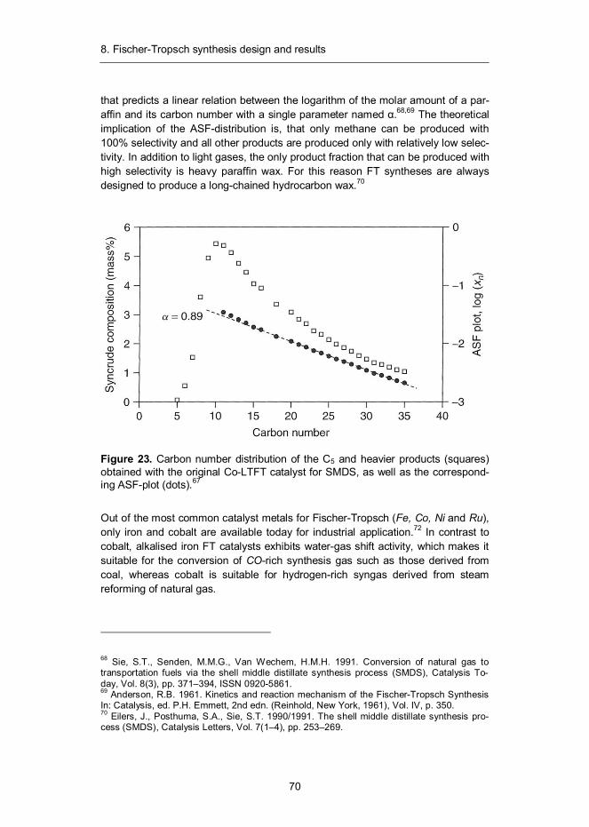
8. Fischer-Tropsch synthesis design and results
70
that predicts a linear relation between the logarithm of the molar amount of a par-affin and its carbon number with a single parameter named .68,69 The theoretical implication of the ASF-distribution is, that only methane can be produced with 100% selectivity and all other products are produced only with relatively low selec-tivity. In addition to light gases, the only product fraction that can be produced with high selectivity is heavy paraffin wax. For this reason FT syntheses are always designed to produce a long-chained hydrocarbon wax.70
Figure 23. Carbon number distribution of the C5 and heavier products (squares) obtained with the original Co-LTFT catalyst for SMDS, as well as the correspond-ing ASF-plot (dots).67
Out of the most common catalyst metals for Fischer-Tropsch (Fe, Co, Ni and Ru), only iron and cobalt are available today for industrial application.72 In contrast to cobalt, alkalised iron FT catalysts exhibits water-gas shift activity, which makes it suitable for the conversion of CO-rich synthesis gas such as those derived from coal, whereas cobalt is suitable for hydrogen-rich syngas derived from steam reforming of natural gas.
68 Sie, S.T., Senden, M.M.G., Van Wechem, H.M.H. 1991. Conversion of natural gas to transportation fuels via the shell middle distillate synthesis process (SMDS), Catalysis To-day, Vol. 8(3), pp. 371–394, ISSN 0920-5861. 69 Anderson, R.B. 1961. Kinetics and reaction mechanism of the Fischer-Tropsch Synthesis In: Catalysis, ed. P.H. Emmett, 2nd edn. (Reinhold, New York, 1961), Vol. IV, p. 350. 70 Eilers, J., Posthuma, S.A., Sie, S.T. 1990/1991. The shell middle distillate synthesis pro-cess (SMDS), Catalysis Letters, Vol. 7(1–4), pp. 253–269.
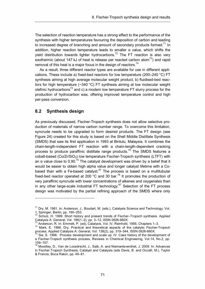
8. Fischer-Tropsch synthesis design and results
71
The selection of reaction temperature has a strong effect to the performance of the synthesis with higher temperatures favouring the deposition of carbon and leading to increased degree of branching and amount of secondary products formed.71 In addition, higher reaction temperature leads to smaller value, which shifts the yield distribution towards lighter hydrocarbons.72 The FT reaction is also very exothermic (about 147 kJ of heat is release per reacted carbon atom73) and rapid removal of this heat is a major focus in the design of reactors.74
As a result, three different reactor types are available for use in different appli-cations. These include a) fixed-bed reactors for low temperature (200–240 °C) FT synthesis aiming at high average molecular weight product, b) fluidised-bed reac-tors for high temperature (~340 °C) FT synthesis aiming at low molecular weight olefinic hydrocarbons72 and c) a modern low temperature FT slurry process for the production of hydrocarbon wax, offering improved temperature control and high per-pass conversion.
8.2 Synthesis design
As previously discussed, Fischer-Tropsch synthesis does not allow selective pro-duction of materials of narrow carbon number range. To overcome this limitation, syncrude needs to be upgraded to form desired products. The FT design (see Figure 24) created for this study is based on the Shell Middle Distillate Synthesis (SMDS) that saw its first application in 1993 at Bintulu, Malaysia. It combines the chain-length-independent FT reaction with a chain-length-dependent cracking process to produce paraffinic distillate range products.70 The SMDS features a cobalt-based (Co/Zr/SiO2) low temperature Fischer-Tropsch synthesis (LTFT) with an value close to 0.90.75 The catalyst development was driven by a belief that it would be easier to obtain high alpha value and longer catalyst lifetime with a Co-based than with a Fe-based catalyst.67 The process is based on a multitubular fixed-bed reactor operated at 200 °C and 30 bar.76 It promotes the production of very paraffinic syncrude with lower concentrations of alkenes and oxygenates than in any other large-scale industrial FT technology.67 Selection of the FT process design was motivated by the partial refining approach of the SMDS where only
71 Dry, M. 1981. In: Anderson, J., Boudart, M. (eds.). Catalysis Science and Technology, Vol. 1, Springer, Berlin, pp. 160–253. 72 Schulz, H. 1999. Short history and present trends of Fischer–Tropsch synthesis. Applied Catalysis A: General, Vol. 186(1–2), pp. 3–12, ISSN 0926-860X. 73 Anderson, R. In: Emmett, P. (ed), Catalysis, Vol. IV, Reinhold, 1956, Chapters 1–3. 74 Mark, E. 1996. Dry, Practical and theoretical aspects of the catalytic Fischer-Tropsch process, Applied Catalysis A: General, Vol. 138(2), pp. 319–344, ISSN 0926-860X. 75 Sie, S. 1998. Process development and scale up: IV. Case history of the development of a Fischer-Tropsch synthesis process, Reviews in Chemical Engineering, Vol.14, No.2, pp. 109–157. 76 Moodley, D., Van de Loosdrecht, J., Saib, A. and Niemantsverdriet, J. 2009. In: Advances in Fischer-Tropsch Synthesis, Catalyst and Catalysis (eds Davis, B. and Occelli, M.), Taylor & Francis, Boca Raton, pp. 49–81.
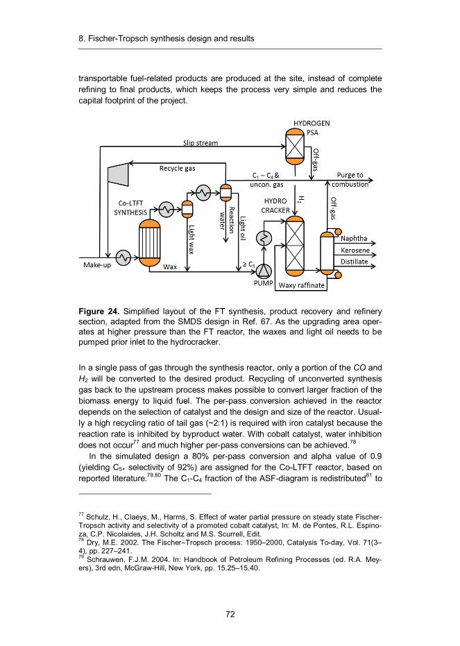
8. Fischer-Tropsch synthesis design and results
72
transportable fuel-related products are produced at the site, instead of complete refining to final products, which keeps the process very simple and reduces the capital footprint of the project.
Figure 24. Simplified layout of the FT synthesis, product recovery and refinery section, adapted from the SMDS design in Ref. 67. As the upgrading area oper-ates at higher pressure than the FT reactor, the waxes and light oil needs to be pumped prior inlet to the hydrocracker.
In a single pass of gas through the synthesis reactor, only a portion of the CO and H2 will be converted to the desired product. Recycling of unconverted synthesis gas back to the upstream process makes possible to convert larger fraction of the biomass energy to liquid fuel. The per-pass conversion achieved in the reactor depends on the selection of catalyst and the design and size of the reactor. Usual-ly a high recycling ratio of tail gas (~2:1) is required with iron catalyst because the reaction rate is inhibited by byproduct water. With cobalt catalyst, water inhibition does not occur77 and much higher per-pass conversions can be achieved.78
In the simulated design a 80% per-pass conversion and alpha value of 0.9 (yielding C5+ selectivity of 92%) are assigned for the Co-LTFT reactor, based on reported literature.79,80 The C1-C4 fraction of the ASF-diagram is redistributed81 to
77 Schulz, H., Claeys, M., Harms, S. Effect of water partial pressure on steady state Fischer-Tropsch activity and selectivity of a promoted cobalt catalyst, In: M. de Pontes, R.L. Espino-za, C.P. Nicolaides, J.H. Scholtz and M.S. Scurrell, Edit. 78 Dry, M.E. 2002. The Fischer–Tropsch process: 1950–2000, Catalysis To-day, Vol. 71(3–4), pp. 227–241. 79 Schrauwen, F.J.M. 2004. In: Handbook of Petroleum Refining Processes (ed. R.A. Mey-ers), 3rd edn, McGraw-Hill, New York, pp. 15.25–15.40.
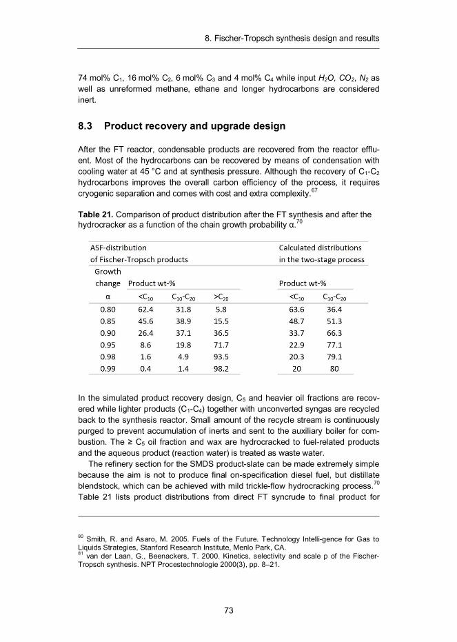
8. Fischer-Tropsch synthesis design and results
73
74 mol% C1, 16 mol% C2, 6 mol% C3 and 4 mol% C4 while input H2O, CO2, N2 as well as unreformed methane, ethane and longer hydrocarbons are considered inert.
8.3 Product recovery and upgrade design
After the FT reactor, condensable products are recovered from the reactor efflu-ent. Most of the hydrocarbons can be recovered by means of condensation with cooling water at 45 °C and at synthesis pressure. Although the recovery of C1-C2 hydrocarbons improves the overall carbon efficiency of the process, it requires cryogenic separation and comes with cost and extra complexity.67
Table 21. Comparison of product distribution after the FT synthesis and after the hydrocracker as a function of the chain growth probability .70
In the simulated product recovery design, C5 and heavier oil fractions are recov-ered while lighter products (C1-C4) together with unconverted syngas are recycled back to the synthesis reactor. Small amount of the recycle stream is continuously purged to prevent accumulation of inerts and sent to the auxiliary boiler for com-bustion. The C5 oil fraction and wax are hydrocracked to fuel-related products and the aqueous product (reaction water) is treated as waste water.
The refinery section for the SMDS product-slate can be made extremely simple because the aim is not to produce final on-specification diesel fuel, but distillate blendstock, which can be achieved with mild trickle-flow hydrocracking process.70 Table 21 lists product distributions from direct FT syncrude to final product for
80 Smith, R. and Asaro, M. 2005. Fuels of the Future. Technology Intelli-gence for Gas to Liquids Strategies, Stanford Research Institute, Menlo Park, CA. 81 van der Laan, G., Beenackers, T. 2000. Kinetics, selectivity and scale p of the Fischer-Tropsch synthesis. NPT Procestechnologie 2000(3), pp. 8–21.
8. Fischer-Tropsch synthesis design and results
74
different values of . It illustrates how the “two-step” process can be elegantly tuned to first minimise the formation of undesired light products (using high alpha) and then selectively hydrocracking the heaviest compounds to yield a three nar-row-carbon-number range fractions (C10-11, C14-16 and C16-17).70
The LTFT wax hydrocracking differs from crude oil hydrocracking in a number of ways.82,83 First of all, it requires milder conditions and consumes much less hydrogen due to the low heteroatom and aromatics content of the LTFT syn-crude.67 In addition, unsulfided noble metal catalysts based on Pt/SiO2-Al2O3 can be used to achieve high selectivity and conversion to distillate, as syncrude itself is essentially sulphur-free.67 In the simulated design, hydrocracking process is oper-ated at 325 °C and 40 bar70 and > 360 °C boiling material (waxy raffinate) is recy-cled to extinction in the hydrocracker. We assume the mass fraction of required hydrogen to hydrocracker feed to be 1% and the gas make from the process to be 2%.67 Depending on the hydrocracking severity, yield ratios of naphtha, kerosene and gas oil can be varied from 15 25 60 (gas oil mode) to 25 50 25 (kerosene mode).68 We assume that the recovery of waste heat provides the needed utilities for the upgrading, leading to zero net parasitic utilities demand for the area.
8.4 Mass and energy balances
This section presents simulation results together with capital costs estimates for five plant configurations suitable for the production of middle distillates from bio-mass via Fischer-Tropsch synthesis. Table 22 shows key parameters of the FT synthesis island for each of the examined plant designs.
For all of the considered designs, 80% per-pass conversion is assumed for the FT reactor. Employing recycle to feed mass ratio of 1 results in 94.4% and 93.8% total CO conversion for the synthesis island for 5 bar and 22 bar front-ends re-spectively. The hydrogen consumption of LTFT wax hydrocracker varies from 4.2 to 4.8 MW for which 7.8 to 8.5 MW of syngas needs to be split to the PSA train. Depending on the design, 13.6 to 15.7 kg/s of saturated admission steam for the turbine is raised in the synthesis at 14 bar and 195 °C. Before injection to turbine this steam is superheated slightly to 245 °C in the auxiliary boiler. The combined off-gas from the synthesis island, compounded of FT recycle purge, PSA off-gas and hydrocracker gasmake, amounts to 30.1 MW, 32.7 MW and 49.7 MW for cases 1 & 2, 3 and 4 & 5, respectively.
82 Sullivan, R.F. and Scott, J.W. 1983. The Development of Hydrocracking, Heterogeneous Catalysis, Vol. 222, Chapter 24, pp. 293–313, ACS Sym-posium Series. 83 Kobolakis, I. and Wojciechowski, B.W. 1985. The catalytic cracking of a fischer-tropsch synthesis product, The Canadian Journal of Chemical Engineering, Vol. 63(2). pp. 269–277.
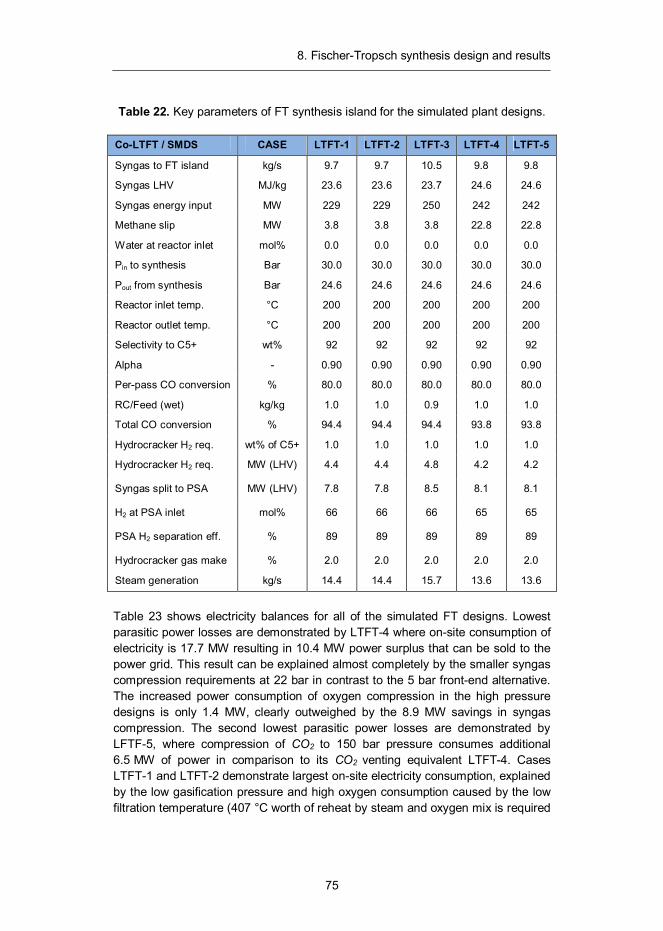
8. Fischer-Tropsch synthesis design and results
75
Table 22. Key parameters of FT synthesis island for the simulated plant designs.
Co-LTFT / SMDS CASE LTFT-1 LTFT-2 LTFT-3 LTFT-4 LTFT-5
Syngas to FT island kg/s 9.7 9.7 10.5 9.8 9.8
Syngas LHV MJ/kg 23.6 23.6 23.7 24.6 24.6
Syngas energy input MW 229 229 250 242 242
Methane slip MW 3.8 3.8 3.8 22.8 22.8
Water at reactor inlet mol% 0.0 0.0 0.0 0.0 0.0
Pin to synthesis Bar 30.0 30.0 30.0 30.0 30.0
Pout from synthesis Bar 24.6 24.6 24.6 24.6 24.6
Reactor inlet temp. °C 200 200 200 200 200
Reactor outlet temp. °C 200 200 200 200 200
Selectivity to C5+ wt% 92 92 92 92 92
Alpha - 0.90 0.90 0.90 0.90 0.90
Per-pass CO conversion % 80.0 80.0 80.0 80.0 80.0
RC/Feed (wet) kg/kg 1.0 1.0 0.9 1.0 1.0
Total CO conversion % 94.4 94.4 94.4 93.8 93.8
Hydrocracker H2 req. wt% of C5+ 1.0 1.0 1.0 1.0 1.0
Hydrocracker H2 req. MW (LHV) 4.4 4.4 4.8 4.2 4.2
Syngas split to PSA MW (LHV) 7.8 7.8 8.5 8.1 8.1
H2 at PSA inlet mol% 66 66 66 65 65
PSA H2 separation eff. % 89 89 89 89 89
Hydrocracker gas make % 2.0 2.0 2.0 2.0 2.0
Steam generation kg/s 14.4 14.4 15.7 13.6 13.6
Table 23 shows electricity balances for all of the simulated FT designs. Lowest parasitic power losses are demonstrated by LTFT-4 where on-site consumption of electricity is 17.7 MW resulting in 10.4 MW power surplus that can be sold to the power grid. This result can be explained almost completely by the smaller syngas compression requirements at 22 bar in contrast to the 5 bar front-end alternative. The increased power consumption of oxygen compression in the high pressure designs is only 1.4 MW, clearly outweighed by the 8.9 MW savings in syngas compression. The second lowest parasitic power losses are demonstrated by LFTF-5, where compression of CO2 to 150 bar pressure consumes additional 6.5 MW of power in comparison to its CO2 venting equivalent LTFT-4. Cases LTFT-1 and LTFT-2 demonstrate largest on-site electricity consumption, explained by the low gasification pressure and high oxygen consumption caused by the low filtration temperature (407 °C worth of reheat by steam and oxygen mix is required
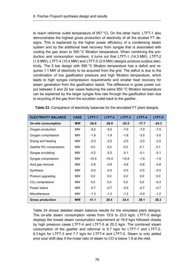
8. Fischer-Tropsch synthesis design and results
76
to reach reformer outlet temperature of 957 °C). On the other hand, LTFT-1 also demonstrates the highest gross production of electricity of all the studied FT de-signs. This is explained by the higher power efficiency of a condensing steam system and by the additional heat recovery from syngas that is associated with cooling the gas down to 550 °C filtration temperature. When combining the pro-duction and consumption numbers, it turns out that LTFT-1 (14.3 MW), LTFT-2 (1.6 MW), LTFT-4 (10.4 MW) and LTFT-5 (3.9 MW) designs produce surplus elec-tricity. The 5 bar design with 850 °C filtration temperature has a deficit and re-quires 1.1 MW of electricity to be acquired from the grid. The deficit is due to the combination of low gasification pressure and high filtration temperature, which leads to high syngas compression requirements and smaller heat recovery for steam generation from the gasification island. The difference in gross power out-put between 5 and 22 bar cases featuring the same 850 °C filtration temperature can be explained by the larger syngas flow rate through the gasification train due to recycling of the gas from the scrubber outlet back to the gasifier.
Table 23. Comparison of electricity balances for the simulated FT plant designs.
ELECTRICITY BALANCE CASE LTFT-1 LTFT-2 LTFT-3 LTFT-4 LTFT-5
On-site consumption MW -26.8 -26.8 -25.5 -17.7 -24.3
Oxygen production MW -9.2 -9.2 -7.9 -7.9 -7.9
Oxygen compression MW -1.9 -1.9 -1.6 -3.0 -3.0
Drying and feeding MW -2.0 -2.0 -2.0 -2.0 -2.0
Gasifier RC compression MW 0.0 0.0 0.0 0.1 0.1
Syngas scrubbing MW -0.2 -0.2 -0.1 -0.1 -0.1
Syngas compression MW -10.4 -10.4 -10.8 -1.9 -1.9
Acid gas removal MW -0.8 -0.8 -0.8 -0.8 -0.8
Synthesis MW -0.5 -0.5 -0.5 -0.5 -0.5
Product upgrading MW 0.0 0.0 0.0 0.0 0.0
CO2 compression MW 0.0 0.0 0.0 0.0 -6.3
Power Island MW -0.7 -0.7 -0.5 -0.7 -0.7
Miscellaneous MW -1.3 -1.3 -1.2 -0.9 -1.2
Gross production MW 41.1 28.5 24.4 28.1 28.2
Table 24 shows detailed steam balance results for the simulated plant designs. The on-site steam consumption varies from 19.9 to 23.0 kg/s. LTFT-3 design displays the lowest steam consumption requirement at 19.9 kg/s followed closely by high pressure cases LTFT-4 and LTFT-5 at 20.2 kg/s. The combined steam consumption of the gasifier and reformer is 9.7 kg/s for LTFT-1 and LTFT-2, 8.3 kg/s for LTFT-3 and 7.7 kg/s for LTFT-4 and LTFT-5. Steam is only added prior sour shift step if the molar ratio of steam to CO is below 1.8 at the inlet.
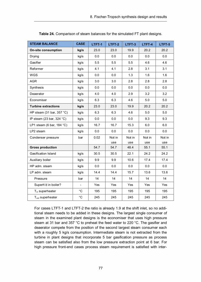
8. Fischer-Tropsch synthesis design and results
77
Table 24. Comparison of steam balances for the simulated FT plant designs.
STEAM BALANCE CASE LTFT-1 LTFT-2 LTFT-3 LTFT-4 LTFT-5
On-site consumption kg/s 23.0 23.0 19.9 20.2 20.2
Drying kg/s 0.0 0.0 0.0 0.0 0.0
Gasifier kg/s 5.5 5.5 5.5 4.6 4.6
Reformer kg/s 4.1 4.1 2.8 3.1 3.1
WGS kg/s 0.0 0.0 1.3 1.6 1.6
AGR kg/s 3.0 3.0 2.8 2.8 2.8
Synthesis kg/s 0.0 0.0 0.0 0.0 0.0
Deaerator kg/s 4.0 4.0 2.9 3.2 3.2
Economiser kg/s 6.3 6.3 4.6 5.0 5.0
Turbine extractions kg/s 23.0 23.0 19.9 20.2 20.2
HP steam (31 bar, 357 °C) kg/s 6.3 6.3 4.6 5.0 5.0
IP steam (23 bar, 324 °C) kg/s 0.0 0.0 0.0 9.3 9.3
LP1 steam (6 bar, 184 °C) kg/s 16.7 16.7 15.3 6.0 6.0
LP2 steam kg/s 0.0 0.0 0.0 0.0 0.0
Condenser pressure bar 0.02 Not in use
Not in use
Not in use
Not in use
Gross production 54.7 54.7 48.4 55.1 55.1
Gasification Island kg/s 30.5 30.5 22.1 24.2 24.2
Auxiliary boiler kg/s 9.9 9.9 10.6 17.4 17.4
HP adm. steam kg/s 0.0 0.0 0.0 0.0 0.0
LP adm. steam kg/s 14.4 14.4 15.7 13.6 13.6
Pressure bar 14 14 14 14 14
Superh’d in boiler? - Yes Yes Yes Yes Yes
Tin superheater °C 195 195 195 195 195
Tout superheater °C 245 245 245 245 245
For cases LTFT-1 and LTFT-2 the ratio is already 1.9 at the shift inlet, so no addi-tional steam needs to be added in these designs. The largest single consumer of steam in the examined plant designs is the economiser that uses high pressure steam at 31 bar and 357 °C to preheat the feed water to 220 °C. The gasifier and deaerator compete from the position of the second largest steam consumer each with a roughly 5 kg/s consumption. Intermediate steam is not extracted from the turbine in plant designs that incorporate 5 bar gasification pressure as process steam can be satisfied also from the low pressure extraction point at 6 bar. For high pressure front-end cases process steam requirement is satisfied with inter-
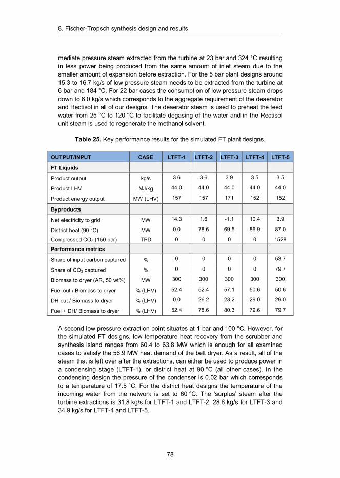
8. Fischer-Tropsch synthesis design and results
78
mediate pressure steam extracted from the turbine at 23 bar and 324 °C resulting in less power being produced from the same amount of inlet steam due to the smaller amount of expansion before extraction. For the 5 bar plant designs around 15.3 to 16.7 kg/s of low pressure steam needs to be extracted from the turbine at 6 bar and 184 °C. For 22 bar cases the consumption of low pressure steam drops down to 6.0 kg/s which corresponds to the aggregate requirement of the deaerator and Rectisol in all of our designs. The deaerator steam is used to preheat the feed water from 25 °C to 120 °C to facilitate degasing of the water and in the Rectisol unit steam is used to regenerate the methanol solvent.
Table 25. Key performance results for the simulated FT plant designs.
OUTPUT/INPUT CASE LTFT-1 LTFT-2 LTFT-3 LTFT-4 LTFT-5
FT Liquids
Product output kg/s 3.6 3.6 3.9 3.5 3.5
Product LHV MJ/kg 44.0 44.0 44.0 44.0 44.0
Product energy output MW (LHV) 157 157 171 152 152
Byproducts
Net electricity to grid MW 14.3 1.6 -1.1 10.4 3.9
District heat (90 °C) MW 0.0 78.6 69.5 86.9 87.0
Compressed CO2 (150 bar) TPD 0 0 0 0 1528
Performance metrics
Share of input carbon captured % 0 0 0 0 53.7
Share of CO2 captured % 0 0 0 0 79.7
Biomass to dryer (AR, 50 wt%) MW 300 300 300 300 300
Fuel out / Biomass to dryer % (LHV) 52.4 52.4 57.1 50.6 50.6
DH out / Biomass to dryer % (LHV) 0.0 26.2 23.2 29.0 29.0
Fuel + DH/ Biomass to dryer % (LHV) 52.4 78.6 80.3 79.6 79.7
A second low pressure extraction point situates at 1 bar and 100 °C. However, for the simulated FT designs, low temperature heat recovery from the scrubber and synthesis island ranges from 60.4 to 63.8 MW which is enough for all examined cases to satisfy the 56.9 MW heat demand of the belt dryer. As a result, all of the steam that is left over after the extractions, can either be used to produce power in a condensing stage (LTFT-1), or district heat at 90 °C (all other cases). In the condensing design the pressure of the condenser is 0.02 bar which corresponds to a temperature of 17.5 °C. For the district heat designs the temperature of the incoming water from the network is set to 60 °C. The ‘surplus’ steam after the turbine extractions is 31.8 kg/s for LTFT-1 and LTFT-2, 28.6 kg/s for LTFT-3 and 34.9 kg/s for LTFT-4 and LTFT-5.
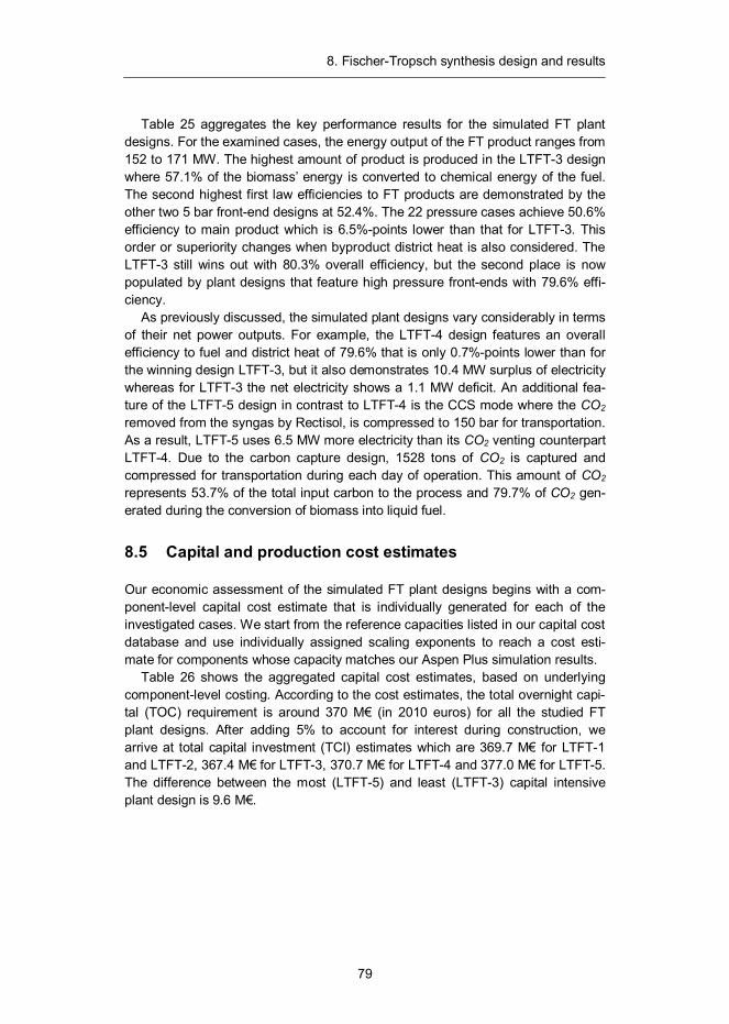
8. Fischer-Tropsch synthesis design and results
79
Table 25 aggregates the key performance results for the simulated FT plant designs. For the examined cases, the energy output of the FT product ranges from 152 to 171 MW. The highest amount of product is produced in the LTFT-3 design where 57.1% of the biomass’ energy is converted to chemical energy of the fuel. The second highest first law efficiencies to FT products are demonstrated by the other two 5 bar front-end designs at 52.4%. The 22 pressure cases achieve 50.6% efficiency to main product which is 6.5%-points lower than that for LTFT-3. This order or superiority changes when byproduct district heat is also considered. The LTFT-3 still wins out with 80.3% overall efficiency, but the second place is now populated by plant designs that feature high pressure front-ends with 79.6% effi-ciency.
As previously discussed, the simulated plant designs vary considerably in terms of their net power outputs. For example, the LTFT-4 design features an overall efficiency to fuel and district heat of 79.6% that is only 0.7%-points lower than for the winning design LTFT-3, but it also demonstrates 10.4 MW surplus of electricity whereas for LTFT-3 the net electricity shows a 1.1 MW deficit. An additional fea-ture of the LTFT-5 design in contrast to LTFT-4 is the CCS mode where the CO2 removed from the syngas by Rectisol, is compressed to 150 bar for transportation. As a result, LTFT-5 uses 6.5 MW more electricity than its CO2 venting counterpart LTFT-4. Due to the carbon capture design, 1528 tons of CO2 is captured and compressed for transportation during each day of operation. This amount of CO2 represents 53.7% of the total input carbon to the process and 79.7% of CO2 gen-erated during the conversion of biomass into liquid fuel.
8.5 Capital and production cost estimates
Our economic assessment of the simulated FT plant designs begins with a com-ponent-level capital cost estimate that is individually generated for each of the investigated cases. We start from the reference capacities listed in our capital cost database and use individually assigned scaling exponents to reach a cost esti-mate for components whose capacity matches our Aspen Plus simulation results.
Table 26 shows the aggregated capital cost estimates, based on underlying component-level costing. According to the cost estimates, the total overnight capi-tal (TOC) requirement is around 370 M€ (in 2010 euros) for all the studied FT plant designs. After adding 5% to account for interest during construction, we arrive at total capital investment (TCI) estimates which are 369.7 M€ for LTFT-1 and LTFT-2, 367.4 M€ for LTFT-3, 370.7 M€ for LTFT-4 and 377.0 M€ for LTFT-5. The difference between the most (LTFT-5) and least (LTFT-3) capital intensive plant design is 9.6 M€.
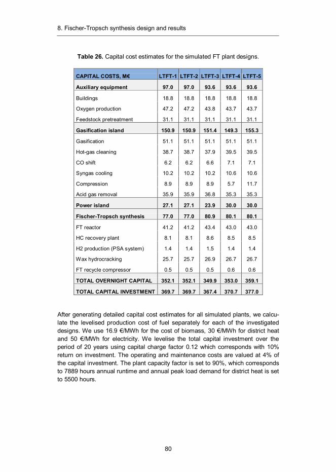
8. Fischer-Tropsch synthesis design and results
80
Table 26. Capital cost estimates for the simulated FT plant designs.
CAPITAL COSTS, M€ LTFT-1 LTFT-2 LTFT-3 LTFT-4 LTFT-5
Auxiliary equipment 97.0 97.0 93.6 93.6 93.6
Buildings 18.8 18.8 18.8 18.8 18.8
Oxygen production 47.2 47.2 43.8 43.7 43.7
Feedstock pretreatment 31.1 31.1 31.1 31.1 31.1
Gasification island 150.9 150.9 151.4 149.3 155.3
Gasification 51.1 51.1 51.1 51.1 51.1
Hot-gas cleaning 38.7 38.7 37.9 39.5 39.5
CO shift 6.2 6.2 6.6 7.1 7.1
Syngas cooling 10.2 10.2 10.2 10.6 10.6
Compression 8.9 8.9 8.9 5.7 11.7
Acid gas removal 35.9 35.9 36.8 35.3 35.3
Power island 27.1 27.1 23.9 30.0 30.0
Fischer-Tropsch synthesis 77.0 77.0 80.9 80.1 80.1
FT reactor 41.2 41.2 43.4 43.0 43.0
HC recovery plant 8.1 8.1 8.6 8.5 8.5
H2 production (PSA system) 1.4 1.4 1.5 1.4 1.4
Wax hydrocracking 25.7 25.7 26.9 26.7 26.7
FT recycle compressor 0.5 0.5 0.5 0.6 0.6
TOTAL OVERNIGHT CAPITAL 352.1 352.1 349.9 353.0 359.1
TOTAL CAPITAL INVESTMENT 369.7 369.7 367.4 370.7 377.0
After generating detailed capital cost estimates for all simulated plants, we calcu-late the levelised production cost of fuel separately for each of the investigated designs. We use 16.9 €/MWh for the cost of biomass, 30 €/MWh for district heat and 50 €/MWh for electricity. We levelise the total capital investment over the period of 20 years using capital charge factor 0.12 which corresponds with 10% return on investment. The operating and maintenance costs are valued at 4% of the capital investment. The plant capacity factor is set to 90%, which corresponds to 7889 hours annual runtime and annual peak load demand for district heat is set to 5500 hours.
8. Fischer-Tropsch synthesis design and results
81
Figure 25. Annual cost estimates (columns) and levelised production costs (dots) for the simulated FT plant designs.
Figure 25 illustrates the levelised annual costs associated with the operation of the plants. The costs are denoted as positive and incomes as negative costs. The income columns are drawn in the figure below the horizontal axis and the costs above. The value of the columns can be read from the primary vertical axis on the left. In addition, we have also added the levelised cost of fuel production (LCOF) as a dot for each of the examined cases. The value of LCOF associated with the cases can be read from the secondary vertical axis on the right. According to the results, the annual costs for all of the studied cases gravitate around 85 M€/a, with LTFT-4 demonstrating the lowest (80.2 M€/a) and LTFT-1 the highest (92.8 M€/a) annual costs. Dividing these costs by the amount of fuel produced annually in the respective plants, we reach production cost estimates that are (in ascending or-der) 64.4 €/MWh (LTFT-3), 66.9 €/MWh (LTFT-4), 68.4 €/MWh (LTFT-2), 69.9 €/MWh (LTFT-5) and 74.9 €/MWh (LTFT-1).
The difference between the lowest and highest annual costs in the simulated designs is 12.6 M€ and the difference between LCOFs is 10.5 €/MWh. The change from condensing mode to CHP mode lowers the LCOF by 6.4 €/MWh and increasing filtration temperature from 550 to 850 °C lowers the LCOF further down by 4.0 €/MWh. The increase of gasification pressure from 5 to 22 bar (assuming previously discussed changes in the performance of the front-end process) actual-ly increases LCOF by 2.5 €/MWh and compressing the separated CO2 stream ready for transportation increases LCOF by 3.0 €/MWh.
9. Methanol-to-gasoline synthesis design and results
82
9. Methanol-to-gasoline synthesis design and results
The most significant development in synthetic fuels technology since the discovery of the Fischer-Tropsch process has been the development of methanol-to-gasoline (MTG) technology by Mobil in the 1970’s.84 In contrast to the product distribution of the FT process, MTG synthesis is very selective producing primarily a finished gasoline blendstock and a byproduct stream that resembles LPG (most-ly propane and butane). The process was demonstrated at industrial scale (15 000 bpd) in New Zealand starting in the mid-1980s using natural gas as feedstock.
9.1 Introduction
The direct conversion of methanol to C2-C10 hydrocarbons catalysed by synthetic zeolite ZSM-5 was discovered in a laboratory by accident. The conversion path is described by the following reaction
/2[2 = + ] , (12)
where CH2 represents gasoline. The reaction is complex, sequential, with steps coupled and highly exothermic.85 The same reaction takes place over many other acidic catalysts as well, but is associated with rapid coking and loss of catalytic activity. The geometrical selectivity of the ZSM-5, however, does not allow the formation of linked aromatic rings that are precursors of coke, resulting in main-tained catalytic activity.86 Another unique characteristic of the product mixture is the abrupt termination in carbon number at around C10 due to the shape-selective nature of the zeolite catalyst. The C5+ product is rich in aromatics and has the
84 Wiley Critical Content – Petroleum Technology. 2007. Vol. 1–2. John Wiley & Sons. 85 Chang, C.D. 1992. The New Zealand Gas-to-Gasoline plant: An engineering tour de force, Catalysis Today, Vol.13(1), pp. 103–111. 86 Wittcoff, H.A., Reuben, B.G., Plotkin, J.S. 2004. Industrial Organic Chemi-cals (2nd Edi-tion). John Wiley & Sons.
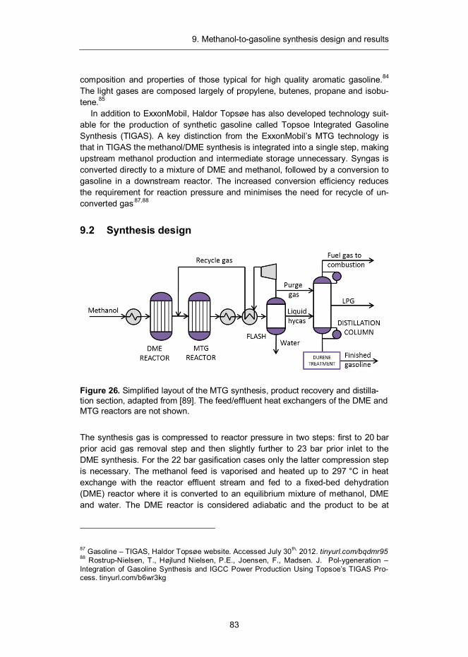
9. Methanol-to-gasoline synthesis design and results
83
composition and properties of those typical for high quality aromatic gasoline.84 The light gases are composed largely of propylene, butenes, propane and isobu-tene.85
In addition to ExxonMobil, Haldor Topsøe has also developed technology suit-able for the production of synthetic gasoline called Topsoe Integrated Gasoline Synthesis (TIGAS). A key distinction from the ExxonMobil’s MTG technology is that in TIGAS the methanol/DME synthesis is integrated into a single step, making upstream methanol production and intermediate storage unnecessary. Syngas is converted directly to a mixture of DME and methanol, followed by a conversion to gasoline in a downstream reactor. The increased conversion efficiency reduces the requirement for reaction pressure and minimises the need for recycle of un-converted gas.87,88
9.2 Synthesis design
Figure 26. Simplified layout of the MTG synthesis, product recovery and distilla-tion section, adapted from [89]. The feed/effluent heat exchangers of the DME and MTG reactors are not shown.
The synthesis gas is compressed to reactor pressure in two steps: first to 20 bar prior acid gas removal step and then slightly further to 23 bar prior inlet to the DME synthesis. For the 22 bar gasification cases only the latter compression step is necessary. The methanol feed is vaporised and heated up to 297 °C in heat exchange with the reactor effluent stream and fed to a fixed-bed dehydration (DME) reactor where it is converted to an equilibrium mixture of methanol, DME and water. The DME reactor is considered adiabatic and the product to be at
87 Gasoline – TIGAS, Haldor Topsøe website. Accessed July 30th, 2012. tinyurl.com/bqdmr95 88 Rostrup-Nielsen, T., Højlund Nielsen, P.E., Joensen, F., Madsen. J. Pol-ygeneration – Integration of Gasoline Synthesis and IGCC Power Production Using Topsoe’s TIGAS Pro-cess. tinyurl.com/b6wr3kg
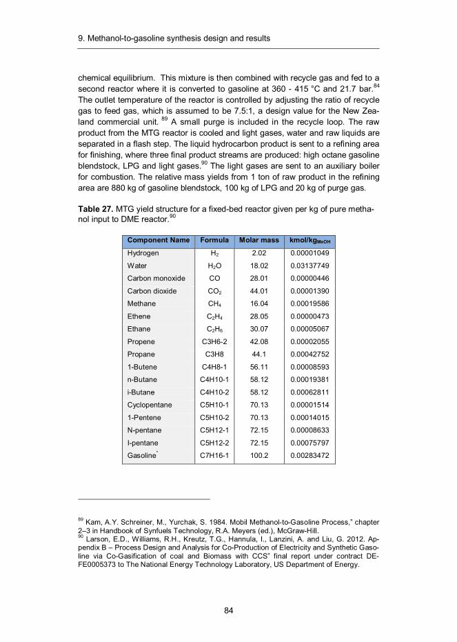
9. Methanol-to-gasoline synthesis design and results
84
chemical equilibrium. This mixture is then combined with recycle gas and fed to a second reactor where it is converted to gasoline at 360 - 415 °C and 21.7 bar.84 The outlet temperature of the reactor is controlled by adjusting the ratio of recycle gas to feed gas, which is assumed to be 7.5:1, a design value for the New Zea-land commercial unit. 89 A small purge is included in the recycle loop. The raw product from the MTG reactor is cooled and light gases, water and raw liquids are separated in a flash step. The liquid hydrocarbon product is sent to a refining area for finishing, where three final product streams are produced: high octane gasoline blendstock, LPG and light gases.90 The light gases are sent to an auxiliary boiler for combustion. The relative mass yields from 1 ton of raw product in the refining area are 880 kg of gasoline blendstock, 100 kg of LPG and 20 kg of purge gas.
Table 27. MTG yield structure for a fixed-bed reactor given per kg of pure metha-nol input to DME reactor.90
Component Name Formula Molar mass kmol/kgMeOH
Hydrogen H2 2.02 0.00001049
Water H2O 18.02 0.03137749
Carbon monoxide CO 28.01 0.00000446
Carbon dioxide CO2 44.01 0.00001390
Methane CH4 16.04 0.00019586
Ethene C2H4 28.05 0.00000473
Ethane C2H6 30.07 0.00005067
Propene C3H6-2 42.08 0.00002055
Propane C3H8 44.1 0.00042752
1-Butene C4H8-1 56.11 0.00008593
n-Butane C4H10-1 58.12 0.00019381
i-Butane C4H10-2 58.12 0.00062811
Cyclopentane C5H10-1 70.13 0.00001514
1-Pentene C5H10-2 70.13 0.00014015
N-pentane C5H12-1 72.15 0.00008633
I-pentane C5H12-2 72.15 0.00075797
Gasoline* C7H16-1 100.2 0.00283472
89 Kam, A.Y. Schreiner, M., Yurchak, S. 1984. Mobil Methanol-to-Gasoline Process,” chapter 2–3 in Handbook of Synfuels Technology, R.A. Meyers (ed.), McGraw-Hill. 90 Larson, E.D., Williams, R.H., Kreutz, T.G., Hannula, I., Lanzini, A. and Liu, G. 2012. Ap-pendix B – Process Design and Analysis for Co-Production of Electricity and Synthetic Gaso-line via Co-Gasification of coal and Biomass with CCS” final report under contract DE-FE0005373 to The National Energy Technology Laboratory, US Department of Energy.
9. Methanol-to-gasoline synthesis design and results
85
One disadvantage of synthetic gasoline, produced by the MTG process, is its relatively high (3–6 wt%) durene content in comparison to conventional (0.2-0.3 wt%) gasoline. Durene has a high melting point and is known to cause carbu-rettor “icing”. To eliminate this problem, durene needs to undergo isomerisation, disproportionation and demethylation in the presence of hydrogen to convert it to isodurene. The required hydrogen can be produced from synthesis gas as exem-plified in our FT synthesis design. However, Larson et al.90 have estimated that the hydrogen requirement of durene treatment is only 0.2 to 0.6 kg of hydrogen per tonne of total gasoline produced, and due to the minuscule amount they have opted not to include this step in their simulation. In our simulation, we have fol-lowed their example.
Due to the proprietary nature of the process, very little information has been published about the performance of the MTG reactor, which complicates the pro-cess simulation effort. For our simulation we have adopted the yield structure (see Table 21) of a fixed-bed MTG reactor as scrutinised and reported by Larson et al. in Ref. 90. We assume that the recovery of waste heat provides the needed utili-ties for the upgrading, leading to zero net parasitic utilities demand for the area.
9.3 Mass and energy balances
This section presents simulation results together with capital costs estimates for five plant configurations suitable for the production of synthetic gasoline from biomass via methanol-to-gasoline synthesis. Table 28 shows key parameters of the methanol-to-gasoline synthesis (MTG) for each of the examined plant designs, the preceding methanol synthesis has the same key parameters at design cases 1 to 5 as discussed in detail in the previous section.
For all the considered designs, inlet conditions for methanol at the MTG syn-thesis inlet are 23 bar and 297 °C. Per-pass conversion of 82% is achieved in the MTG synthesis. Using a large recycle to feed ratio of 7.5 the total CO conversion in the synthesis island can be increased to almost complete 100% for all investi-gated designs. Depending on the case, 5.2 to 6.0 kg/s or saturated high pressure admission steam is raised on the MTG synthesis at 100 bar and 390 °C. This comes in addition to the 9.9 to 11.4 kg/s of low pressure admission steam is raised in the methanol synthesis at 43 bar and 255 °C. Before injection to turbine this steam is superheated to 500 °C and mixed with the main process steam. The low pressure admission steam from the methanol synthesis is superheated only slight-ly to 305 °C in order to avoid condensation during injection into the turbine. The combined off-gas from the both synthesis islands amounts to 26.6 MW, 28.8 MW and 50.7 MW for cases 1 & 2, 3 and 4 & 5, respectively.
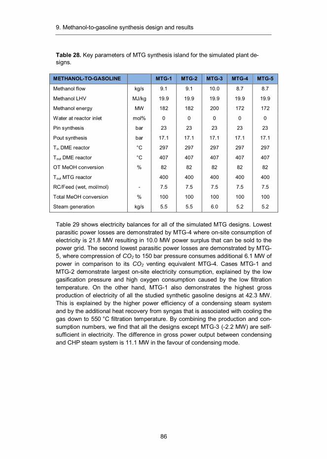
9. Methanol-to-gasoline synthesis design and results
86
Table 28. Key parameters of MTG synthesis island for the simulated plant de-signs.
METHANOL-TO-GASOLINE MTG-1 MTG-2 MTG-3 MTG-4 MTG-5
Methanol flow kg/s 9.1 9.1 10.0 8.7 8.7
Methanol LHV MJ/kg 19.9 19.9 19.9 19.9 19.9
Methanol energy MW 182 182 200 172 172
Water at reactor inlet mol% 0 0 0 0 0
Pin synthesis bar 23 23 23 23 23
Pout synthesis bar 17.1 17.1 17.1 17.1 17.1
Tin DME reactor °C 297 297 297 297 297
Tout DME reactor °C 407 407 407 407 407
OT MeOH conversion % 82 82 82 82 82
Tout MTG reactor 400 400 400 400 400
RC/Feed (wet, mol/mol) - 7.5 7.5 7.5 7.5 7.5
Total MeOH conversion % 100 100 100 100 100
Steam generation kg/s 5.5 5.5 6.0 5.2 5.2
Table 29 shows electricity balances for all of the simulated MTG designs. Lowest parasitic power losses are demonstrated by MTG-4 where on-site consumption of electricity is 21.8 MW resulting in 10.0 MW power surplus that can be sold to the power grid. The second lowest parasitic power losses are demonstrated by MTG-5, where compression of CO2 to 150 bar pressure consumes additional 6.1 MW of power in comparison to its CO2 venting equivalent MTG-4. Cases MTG-1 and MTG-2 demonstrate largest on-site electricity consumption, explained by the low gasification pressure and high oxygen consumption caused by the low filtration temperature. On the other hand, MTG-1 also demonstrates the highest gross production of electricity of all the studied synthetic gasoline designs at 42.3 MW. This is explained by the higher power efficiency of a condensing steam system and by the additional heat recovery from syngas that is associated with cooling the gas down to 550 °C filtration temperature. By combining the production and con-sumption numbers, we find that all the designs except MTG-3 (-2.2 MW) are self-sufficient in electricity. The difference in gross power output between condensing and CHP steam system is 11.1 MW in the favour of condensing mode.
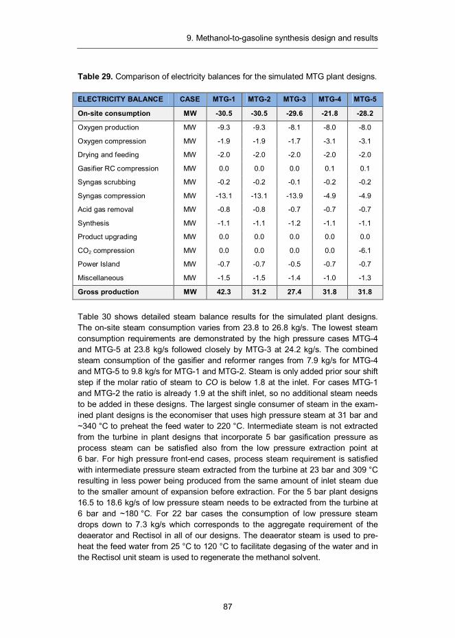
9. Methanol-to-gasoline synthesis design and results
87
Table 29. Comparison of electricity balances for the simulated MTG plant designs.
ELECTRICITY BALANCE CASE MTG-1 MTG-2 MTG-3 MTG-4 MTG-5
On-site consumption MW -30.5 -30.5 -29.6 -21.8 -28.2
Oxygen production MW -9.3 -9.3 -8.1 -8.0 -8.0
Oxygen compression MW -1.9 -1.9 -1.7 -3.1 -3.1
Drying and feeding MW -2.0 -2.0 -2.0 -2.0 -2.0
Gasifier RC compression MW 0.0 0.0 0.0 0.1 0.1
Syngas scrubbing MW -0.2 -0.2 -0.1 -0.2 -0.2
Syngas compression MW -13.1 -13.1 -13.9 -4.9 -4.9
Acid gas removal MW -0.8 -0.8 -0.7 -0.7 -0.7
Synthesis MW -1.1 -1.1 -1.2 -1.1 -1.1
Product upgrading MW 0.0 0.0 0.0 0.0 0.0
CO2 compression MW 0.0 0.0 0.0 0.0 -6.1
Power Island MW -0.7 -0.7 -0.5 -0.7 -0.7
Miscellaneous MW -1.5 -1.5 -1.4 -1.0 -1.3
Gross production MW 42.3 31.2 27.4 31.8 31.8
Table 30 shows detailed steam balance results for the simulated plant designs. The on-site steam consumption varies from 23.8 to 26.8 kg/s. The lowest steam consumption requirements are demonstrated by the high pressure cases MTG-4 and MTG-5 at 23.8 kg/s followed closely by MTG-3 at 24.2 kg/s. The combined steam consumption of the gasifier and reformer ranges from 7.9 kg/s for MTG-4 and MTG-5 to 9.8 kg/s for MTG-1 and MTG-2. Steam is only added prior sour shift step if the molar ratio of steam to CO is below 1.8 at the inlet. For cases MTG-1 and MTG-2 the ratio is already 1.9 at the shift inlet, so no additional steam needs to be added in these designs. The largest single consumer of steam in the exam-ined plant designs is the economiser that uses high pressure steam at 31 bar and ~340 °C to preheat the feed water to 220 °C. Intermediate steam is not extracted from the turbine in plant designs that incorporate 5 bar gasification pressure as process steam can be satisfied also from the low pressure extraction point at 6 bar. For high pressure front-end cases, process steam requirement is satisfied with intermediate pressure steam extracted from the turbine at 23 bar and 309 °C resulting in less power being produced from the same amount of inlet steam due to the smaller amount of expansion before extraction. For the 5 bar plant designs 16.5 to 18.6 kg/s of low pressure steam needs to be extracted from the turbine at 6 bar and ~180 °C. For 22 bar cases the consumption of low pressure steam drops down to 7.3 kg/s which corresponds to the aggregate requirement of the deaerator and Rectisol in all of our designs. The deaerator steam is used to pre-heat the feed water from 25 °C to 120 °C to facilitate degasing of the water and in the Rectisol unit steam is used to regenerate the methanol solvent.
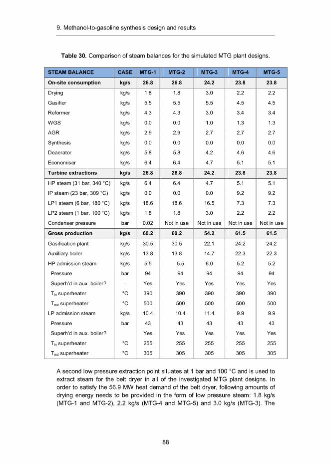
9. Methanol-to-gasoline synthesis design and results
88
Table 30. Comparison of steam balances for the simulated MTG plant designs.
STEAM BALANCE CASE MTG-1 MTG-2 MTG-3 MTG-4 MTG-5
On-site consumption kg/s 26.8 26.8 24.2 23.8 23.8
Drying kg/s 1.8 1.8 3.0 2.2 2.2
Gasifier kg/s 5.5 5.5 5.5 4.5 4.5
Reformer kg/s 4.3 4.3 3.0 3.4 3.4
WGS kg/s 0.0 0.0 1.0 1.3 1.3
AGR kg/s 2.9 2.9 2.7 2.7 2.7
Synthesis kg/s 0.0 0.0 0.0 0.0 0.0
Deaerator kg/s 5.8 5.8 4.2 4.6 4.6
Economiser kg/s 6.4 6.4 4.7 5.1 5.1
Turbine extractions kg/s 26.8 26.8 24.2 23.8 23.8
HP steam (31 bar, 340 °C) kg/s 6.4 6.4 4.7 5.1 5.1
IP steam (23 bar, 309 °C) kg/s 0.0 0.0 0.0 9.2 9.2
LP1 steam (6 bar, 180 °C) kg/s 18.6 18.6 16.5 7.3 7.3
LP2 steam (1 bar, 100 °C) kg/s 1.8 1.8 3.0 2.2 2.2
Condenser pressure bar 0.02 Not in use Not in use Not in use Not in use
Gross production kg/s 60.2 60.2 54.2 61.5 61.5
Gasification plant kg/s 30.5 30.5 22.1 24.2 24.2
Auxiliary boiler kg/s 13.8 13.8 14.7 22.3 22.3
HP admission steam kg/s 5.5 5.5 6.0 5.2 5.2
Pressure bar 94 94 94 94 94
Superh'd in aux. boiler? - Yes Yes Yes Yes Yes
Tin superheater °C 390 390 390 390 390
Tout superheater °C 500 500 500 500 500
LP admission steam kg/s 10.4 10.4 11.4 9.9 9.9
Pressure bar 43 43 43 43 43
Superh'd in aux. boiler? Yes Yes Yes Yes Yes
Tin superheater °C 255 255 255 255 255
Tout superheater °C 305 305 305 305 305
A second low pressure extraction point situates at 1 bar and 100 °C and is used to extract steam for the belt dryer in all of the investigated MTG plant designs. In order to satisfy the 56.9 MW heat demand of the belt dryer, following amounts of drying energy needs to be provided in the form of low pressure steam: 1.8 kg/s (MTG-1 and MTG-2), 2.2 kg/s (MTG-4 and MTG-5) and 3.0 kg/s (MTG-3). The
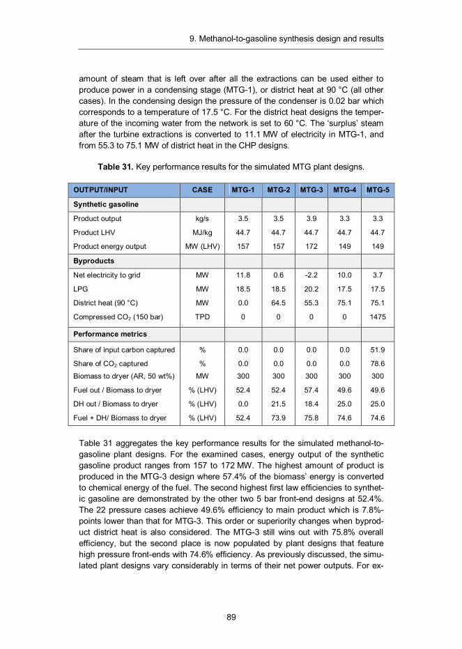
9. Methanol-to-gasoline synthesis design and results
89
amount of steam that is left over after all the extractions can be used either to produce power in a condensing stage (MTG-1), or district heat at 90 °C (all other cases). In the condensing design the pressure of the condenser is 0.02 bar which corresponds to a temperature of 17.5 °C. For the district heat designs the temper-ature of the incoming water from the network is set to 60 °C. The ‘surplus’ steam after the turbine extractions is converted to 11.1 MW of electricity in MTG-1, and from 55.3 to 75.1 MW of district heat in the CHP designs.
Table 31. Key performance results for the simulated MTG plant designs.
OUTPUT/INPUT CASE MTG-1 MTG-2 MTG-3 MTG-4 MTG-5
Synthetic gasoline
Product output kg/s 3.5 3.5 3.9 3.3 3.3
Product LHV MJ/kg 44.7 44.7 44.7 44.7 44.7
Product energy output MW (LHV) 157 157 172 149 149
Byproducts
Net electricity to grid MW 11.8 0.6 -2.2 10.0 3.7
LPG MW 18.5 18.5 20.2 17.5 17.5
District heat (90 °C) MW 0.0 64.5 55.3 75.1 75.1
Compressed CO2 (150 bar) TPD 0 0 0 0 1475
Performance metrics
Share of input carbon captured % 0.0 0.0 0.0 0.0 51.9
Share of CO2 captured % 0.0 0.0 0.0 0.0 78.6
Biomass to dryer (AR, 50 wt%) MW 300 300 300 300 300
Fuel out / Biomass to dryer % (LHV) 52.4 52.4 57.4 49.6 49.6
DH out / Biomass to dryer % (LHV) 0.0 21.5 18.4 25.0 25.0
Fuel + DH/ Biomass to dryer % (LHV) 52.4 73.9 75.8 74.6 74.6
Table 31 aggregates the key performance results for the simulated methanol-to-gasoline plant designs. For the examined cases, energy output of the synthetic gasoline product ranges from 157 to 172 MW. The highest amount of product is produced in the MTG-3 design where 57.4% of the biomass’ energy is converted to chemical energy of the fuel. The second highest first law efficiencies to synthet-ic gasoline are demonstrated by the other two 5 bar front-end designs at 52.4%. The 22 pressure cases achieve 49.6% efficiency to main product which is 7.8%-points lower than that for MTG-3. This order or superiority changes when byprod-uct district heat is also considered. The MTG-3 still wins out with 75.8% overall efficiency, but the second place is now populated by plant designs that feature high pressure front-ends with 74.6% efficiency. As previously discussed, the simu-lated plant designs vary considerably in terms of their net power outputs. For ex-
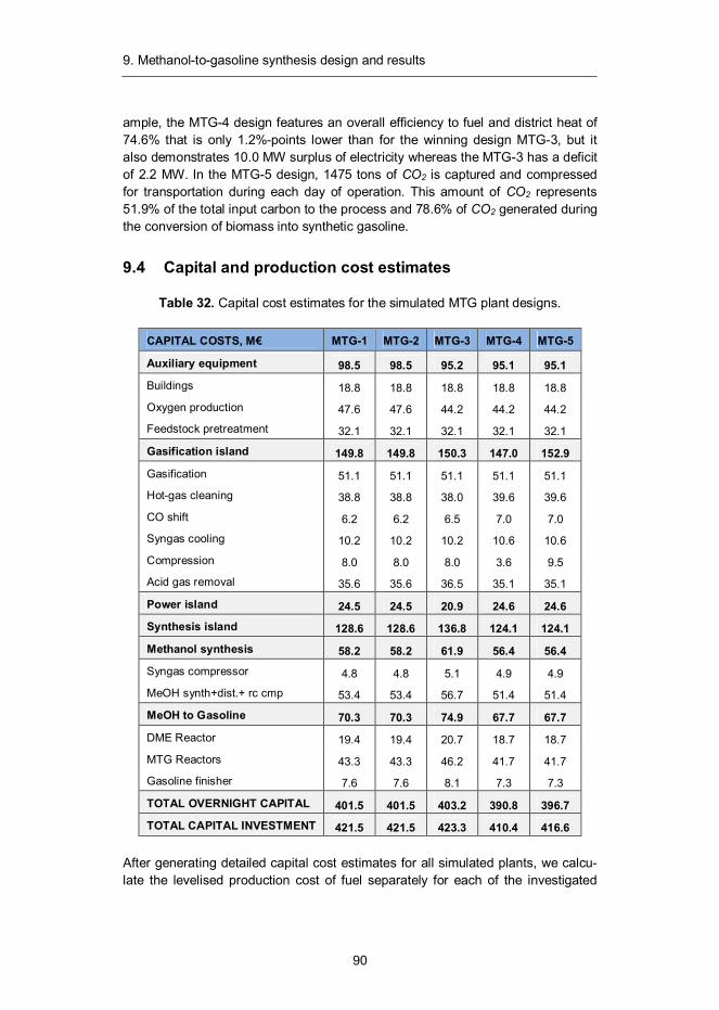
9. Methanol-to-gasoline synthesis design and results
90
ample, the MTG-4 design features an overall efficiency to fuel and district heat of 74.6% that is only 1.2%-points lower than for the winning design MTG-3, but it also demonstrates 10.0 MW surplus of electricity whereas the MTG-3 has a deficit of 2.2 MW. In the MTG-5 design, 1475 tons of CO2 is captured and compressed for transportation during each day of operation. This amount of CO2 represents 51.9% of the total input carbon to the process and 78.6% of CO2 generated during the conversion of biomass into synthetic gasoline.
9.4 Capital and production cost estimates
Table 32. Capital cost estimates for the simulated MTG plant designs.
CAPITAL COSTS, M€ MTG-1 MTG-2 MTG-3 MTG-4 MTG-5
Auxiliary equipment 98.5 98.5 95.2 95.1 95.1
Buildings 18.8 18.8 18.8 18.8 18.8
Oxygen production 47.6 47.6 44.2 44.2 44.2
Feedstock pretreatment 32.1 32.1 32.1 32.1 32.1
Gasification island 149.8 149.8 150.3 147.0 152.9
Gasification 51.1 51.1 51.1 51.1 51.1
Hot-gas cleaning 38.8 38.8 38.0 39.6 39.6
CO shift 6.2 6.2 6.5 7.0 7.0
Syngas cooling 10.2 10.2 10.2 10.6 10.6
Compression 8.0 8.0 8.0 3.6 9.5
Acid gas removal 35.6 35.6 36.5 35.1 35.1
Power island 24.5 24.5 20.9 24.6 24.6
Synthesis island 128.6 128.6 136.8 124.1 124.1
Methanol synthesis 58.2 58.2 61.9 56.4 56.4
Syngas compressor 4.8 4.8 5.1 4.9 4.9
MeOH synth+dist.+ rc cmp 53.4 53.4 56.7 51.4 51.4
MeOH to Gasoline 70.3 70.3 74.9 67.7 67.7
DME Reactor 19.4 19.4 20.7 18.7 18.7
MTG Reactors 43.3 43.3 46.2 41.7 41.7
Gasoline finisher 7.6 7.6 8.1 7.3 7.3
TOTAL OVERNIGHT CAPITAL 401.5 401.5 403.2 390.8 396.7
TOTAL CAPITAL INVESTMENT 421.5 421.5 423.3 410.4 416.6 After generating detailed capital cost estimates for all simulated plants, we calcu-late the levelised production cost of fuel separately for each of the investigated
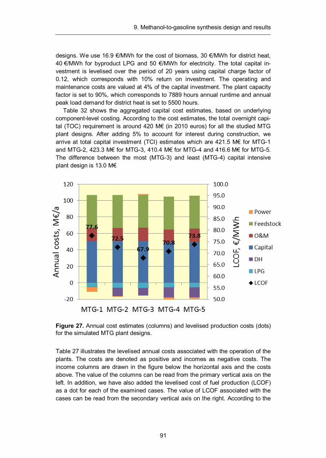
9. Methanol-to-gasoline synthesis design and results
91
designs. We use 16.9 €/MWh for the cost of biomass, 30 €/MWh for district heat, 40 €/MWh for byproduct LPG and 50 €/MWh for electricity. The total capital in-vestment is levelised over the period of 20 years using capital charge factor of 0.12, which corresponds with 10% return on investment. The operating and maintenance costs are valued at 4% of the capital investment. The plant capacity factor is set to 90%, which corresponds to 7889 hours annual runtime and annual peak load demand for district heat is set to 5500 hours.
Table 32 shows the aggregated capital cost estimates, based on underlying component-level costing. According to the cost estimates, the total overnight capi-tal (TOC) requirement is around 420 M€ (in 2010 euros) for all the studied MTG plant designs. After adding 5% to account for interest during construction, we arrive at total capital investment (TCI) estimates which are 421.5 M€ for MTG-1 and MTG-2, 423.3 M€ for MTG-3, 410.4 M€ for MTG-4 and 416.6 M€ for MTG-5. The difference between the most (MTG-3) and least (MTG-4) capital intensive plant design is 13.0 M€
Figure 27. Annual cost estimates (columns) and levelised production costs (dots) for the simulated MTG plant designs.
Table 27 illustrates the levelised annual costs associated with the operation of the plants. The costs are denoted as positive and incomes as negative costs. The income columns are drawn in the figure below the horizontal axis and the costs above. The value of the columns can be read from the primary vertical axis on the left. In addition, we have also added the levelised cost of fuel production (LCOF) as a dot for each of the examined cases. The value of LCOF associated with the cases can be read from the secondary vertical axis on the right. According to the
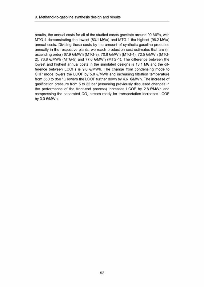
9. Methanol-to-gasoline synthesis design and results
92
results, the annual costs for all of the studied cases gravitate around 90 M€/a, with MTG-4 demonstrating the lowest (83.1 M€/a) and MTG-1 the highest (96.2 M€/a) annual costs. Dividing these costs by the amount of synthetic gasoline produced annually in the respective plants, we reach production cost estimates that are (in ascending order) 67.9 €/MWh (MTG-3), 70.8 €/MWh (MTG-4), 72.5 €/MWh (MTG-2), 73.8 €/MWh (MTG-5) and 77.6 €/MWh (MTG-1). The difference between the lowest and highest annual costs in the simulated designs is 13.1 M€ and the dif-ference between LCOFs is 9.6 €/MWh. The change from condensing mode to CHP mode lowers the LCOF by 5.0 €/MWh and increasing filtration temperature from 550 to 850 °C lowers the LCOF further down by 4.6 €/MWh. The increase of gasification pressure from 5 to 22 bar (assuming previously discussed changes in the performance of the front-end process) increases LCOF by 2.8 €/MWh and compressing the separated CO2 stream ready for transportation increases LCOF by 3.0 €/MWh.
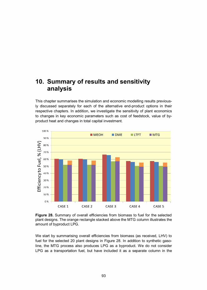
10. Summary of results and sensitivity analysis
93
10. Summary of results and sensitivity analysis
This chapter summarises the simulation and economic modelling results previous-ly discussed separately for each of the alternative end-product options in their respective chapters. In addition, we investigate the sensitivity of plant economics to changes in key economic parameters such as cost of feedstock, value of by-product heat and changes in total capital investment.
Figure 28. Summary of overall efficiencies from biomass to fuel for the selected plant designs. The orange rectangle stacked above the MTG column illustrates the amount of byproduct LPG.
We start by summarising overall efficiencies from biomass (as received, LHV) to fuel for the selected 20 plant designs in Figure 28. In addition to synthetic gaso-line, the MTG process also produces LPG as a byproduct. We do not consider LPG as a transportation fuel, but have included it as a separate column in the
10. Summary of results and sensitivity analysis
94
figure to illustrate its share in the overall picture. In the economic analysis, LPG is considered as a saleable product together with district heat and power.
Judging from the figure, it can be seen that for all of the studied cases, metha-nol and DME systematically yield highest (range 56.1–66.7%) and LTFT and MTG lowest (range 49.6–57.4%) efficiencies to fuel. However, the differences between methanol and DME are small (range 0.6–1.3%-points), as are differences between FT liquids and synthetic gasoline (range 0.0–1.1%-points). For all products, the best overall efficiencies are reached with case 3 front-end design that features 5 bar gasification with 850 °C filtration. The second best overall efficiencies are achieved with design cases 1 and 2 that feature 5 bar/550 °C front-end while high-pressure gasification front-end systematically yield lowest efficiencies to fuel.
Figure 29. Overall efficiencies from biomass to fuel and byproduct district heat for the selected plant designs. The MTG fuel efficiency column excludes LPG.
We then combine the efficiency to district heat with the efficiency to fuel in Figure 29. Judging from the results, it is possible to achieve 11 to 29%-points increase in the combined efficiency compared to condensing steam system designs. The largest amount of byproduct heat is produced by the LTFT plant designs where 23 to 29% of the input biomass’ energy is converted to district heat. The lowest amount of byproduct heat is produced in the methanol plants with a range of 11 to 19%. Considering the overall efficiency to fuel and district heat together, the differ-
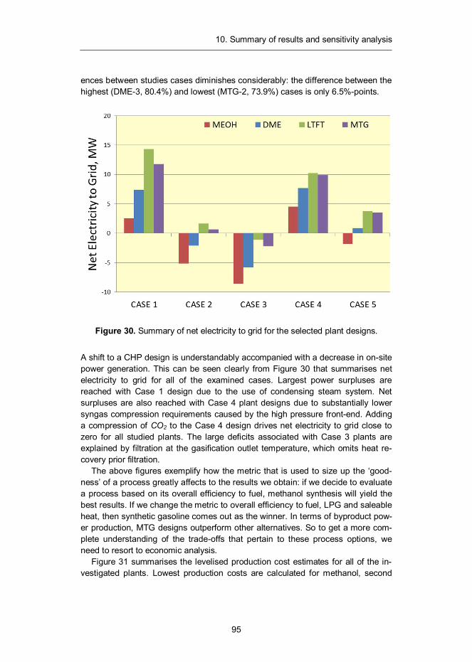
10. Summary of results and sensitivity analysis
95
ences between studies cases diminishes considerably: the difference between the highest (DME-3, 80.4%) and lowest (MTG-2, 73.9%) cases is only 6.5%-points.
Figure 30. Summary of net electricity to grid for the selected plant designs.
A shift to a CHP design is understandably accompanied with a decrease in on-site power generation. This can be seen clearly from Figure 30 that summarises net electricity to grid for all of the examined cases. Largest power surpluses are reached with Case 1 design due to the use of condensing steam system. Net surpluses are also reached with Case 4 plant designs due to substantially lower syngas compression requirements caused by the high pressure front-end. Adding a compression of CO2 to the Case 4 design drives net electricity to grid close to zero for all studied plants. The large deficits associated with Case 3 plants are explained by filtration at the gasification outlet temperature, which omits heat re-covery prior filtration.
The above figures exemplify how the metric that is used to size up the ‘good-ness’ of a process greatly affects to the results we obtain: if we decide to evaluate a process based on its overall efficiency to fuel, methanol synthesis will yield the best results. If we change the metric to overall efficiency to fuel, LPG and saleable heat, then synthetic gasoline comes out as the winner. In terms of byproduct pow-er production, MTG designs outperform other alternatives. So to get a more com-plete understanding of the trade-offs that pertain to these process options, we need to resort to economic analysis.
Figure 31 summarises the levelised production cost estimates for all of the in-vestigated plants. Lowest production costs are calculated for methanol, second
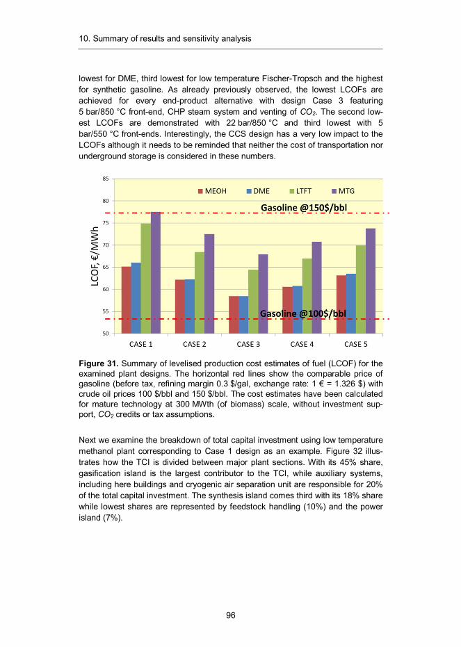
10. Summary of results and sensitivity analysis
96
lowest for DME, third lowest for low temperature Fischer-Tropsch and the highest for synthetic gasoline. As already previously observed, the lowest LCOFs are achieved for every end-product alternative with design Case 3 featuring 5 bar/850 °C front-end, CHP steam system and venting of CO2. The second low-est LCOFs are demonstrated with 22 bar/850 °C and third lowest with 5 bar/550 °C front-ends. Interestingly, the CCS design has a very low impact to the LCOFs although it needs to be reminded that neither the cost of transportation nor underground storage is considered in these numbers.
Figure 31. Summary of levelised production cost estimates of fuel (LCOF) for the examined plant designs. The horizontal red lines show the comparable price of gasoline (before tax, refining margin 0.3 $/gal, exchange rate: 1 € = 1.326 $) with crude oil prices 100 $/bbl and 150 $/bbl. The cost estimates have been calculated for mature technology at 300 MWth (of biomass) scale, without investment sup-port, CO2 credits or tax assumptions.
Next we examine the breakdown of total capital investment using low temperature methanol plant corresponding to Case 1 design as an example. Figure 32 illus-trates how the TCI is divided between major plant sections. With its 45% share, gasification island is the largest contributor to the TCI, while auxiliary systems, including here buildings and cryogenic air separation unit are responsible for 20% of the total capital investment. The synthesis island comes third with its 18% share while lowest shares are represented by feedstock handling (10%) and the power island (7%).
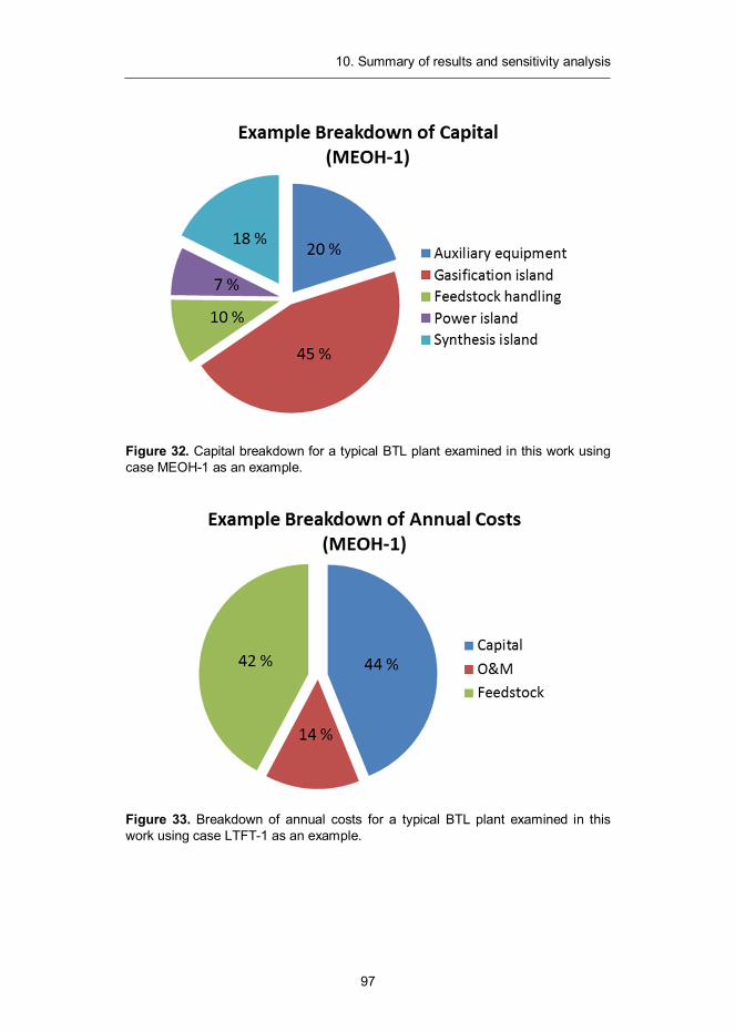
10. Summary of results and sensitivity analysis
97
Figure 32. Capital breakdown for a typical BTL plant examined in this work using case MEOH-1 as an example.
Figure 33. Breakdown of annual costs for a typical BTL plant examined in this work using case LTFT-1 as an example.
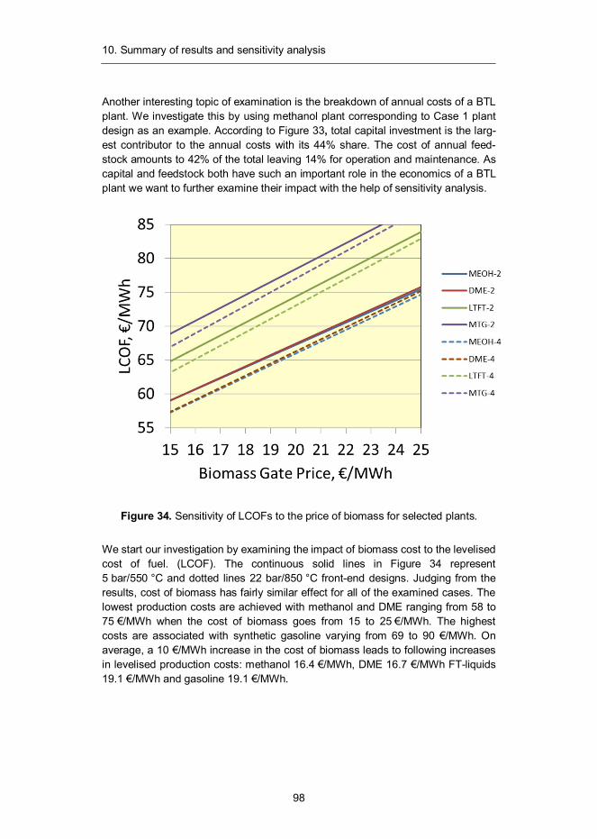
10. Summary of results and sensitivity analysis
98
Another interesting topic of examination is the breakdown of annual costs of a BTL plant. We investigate this by using methanol plant corresponding to Case 1 plant design as an example. According to Figure 33, total capital investment is the larg-est contributor to the annual costs with its 44% share. The cost of annual feed-stock amounts to 42% of the total leaving 14% for operation and maintenance. As capital and feedstock both have such an important role in the economics of a BTL plant we want to further examine their impact with the help of sensitivity analysis.
Figure 34. Sensitivity of LCOFs to the price of biomass for selected plants.
We start our investigation by examining the impact of biomass cost to the levelised cost of fuel. (LCOF). The continuous solid lines in Figure 34 represent 5 bar/550 °C and dotted lines 22 bar/850 °C front-end designs. Judging from the results, cost of biomass has fairly similar effect for all of the examined cases. The lowest production costs are achieved with methanol and DME ranging from 58 to 75 €/MWh when the cost of biomass goes from 15 to 25 €/MWh. The highest costs are associated with synthetic gasoline varying from 69 to 90 €/MWh. On average, a 10 €/MWh increase in the cost of biomass leads to following increases in levelised production costs: methanol 16.4 €/MWh, DME 16.7 €/MWh FT-liquids 19.1 €/MWh and gasoline 19.1 €/MWh.
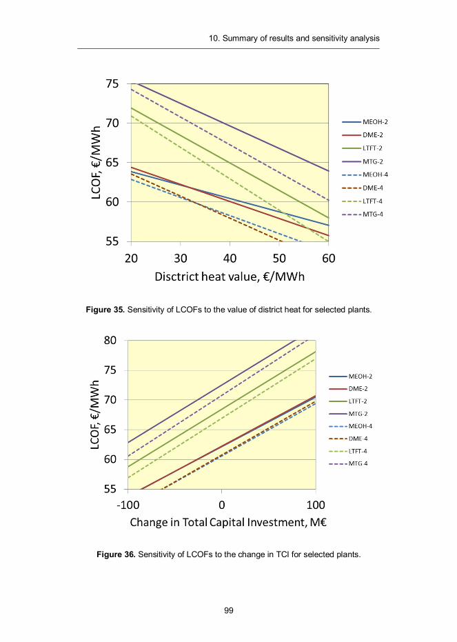
10. Summary of results and sensitivity analysis
99
Figure 35. Sensitivity of LCOFs to the value of district heat for selected plants.
Figure 36. Sensitivity of LCOFs to the change in TCI for selected plants.
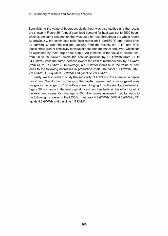
10. Summary of results and sensitivity analysis
100
Sensitivity to the value of byproduct district heat was also studied and the results are shown in Figure 35. Annual peak load demand for heat was set to 5500 hours, which is the same assumption that was used for heat throughout the whole report. As previously, the continuous solid lines represent 5 bar/550 °C and dotted lines 22 bar/850 °C front-end designs. Judging from the results, the LTFT and MTG plants show greater sensitivity to value of heat than methanol and DME, which can be explained by their larger heat output. An increase in the value of district heat from 20 to 60 €/MWh lowers the cost of gasoline by 12 €/MWh (from 76 to 64 €/MWh) while the same increase lowers the cost of methanol only by 7 €/MWh (from 64 to 57 €/MWh). On average, a 10 €/MWh increase in the value of heat leads to the following decreases in production costs: methanol 1.7 €/MWh, DME 2.2 €/MWh, FT-liquids 3.5 €/MWh and gasoline 2.9 €/MWh.
Finally, we also want to study the sensitivity of LCOFs to the changes in capital investment. We do this by changing the capital requirement of investigated plant designs in the range of ±100 million euros. Judging from the results, illustrated in Figure 36, a change in the total capital investment has fairly similar effect for all of the examined cases. On average, a 50 million euros increase in capital leads to the following increases in the LCOFs: methanol 4.2 €/MWh, DME 4.2 €/MWh, FT-liquids 4.8 €/MWh and gasoline 4.8 €/MWh.
11. Discussion
101
11. Discussion
Transportation causes nearly one quarter of global energy-related CO2 emissions and liquid biofuels can play an important part in mitigating them. In addition, they are almost the only option for the decarbonisation of heavy duty vehicles and air traffic. As a result, 52 countries have set targets and mandates for biofuels. The bulk of these mandates come from the EU-27 area where 10% of renewables content is required in traffic by 2020 by all member states. Other major mandates are set in the US, China and Brazil, where targets are in the range of 15–20% by 2020–22.
The principal liquid biofuel in the world in 2012 is still ethanol. The global pro-duction of fuel ethanol was 85 billion litres in 2011 and 87% of it was produced by USA (from corn) and Brazil (from sugarcane). Production of liquid fuels from feed-stocks used mainly for food and feed remains a controversial issue and increasing pressure exists to shift from starch-based conventional biofuels to more advanced substitutes. These so called second generation synthetic biofuels, made from non-edible feedstocks, can be produced with lower life-cycle CO2 emissions and are cleaner than most conventional fossil fuels they’ll replace, having essentially zero levels of sulphur and other contaminants.
In the previous chapters, we have examined the technical and economic feasi-bility of 20 individual plant designs, capable of converting biomass into methanol, dimethyl ether, Fischer-Tropsch liquids or synthetic gasoline. All of the investigat-ed plant designs were based on pressurised fluidised-bed oxygen gasification that has been the focus of extensive research and development in Finland during the recent years. Our analysis shows, that BTL plants, with the kind of performance and cost parameters assumed in this work, are able to produce sustainable low-carbon fuels on parity with 110 to 150 $/bbl crude oil price (see Figure 37). The lower end of the production cost estimates are close to long-term price forecasts for crude oil and would not therefore require substantial incentives to break even. However, pioneering plants are likely to have much higher costs than plants exam-ined in this report and significant public support is required to deploy this technol-ogy at scale.
It is worth pointing out that although FT liquids and synthetic gasoline were found to be more expensive in relation to methanol and DME, important differ-ences exist in the properties of these fuels and therefore they should not be com-
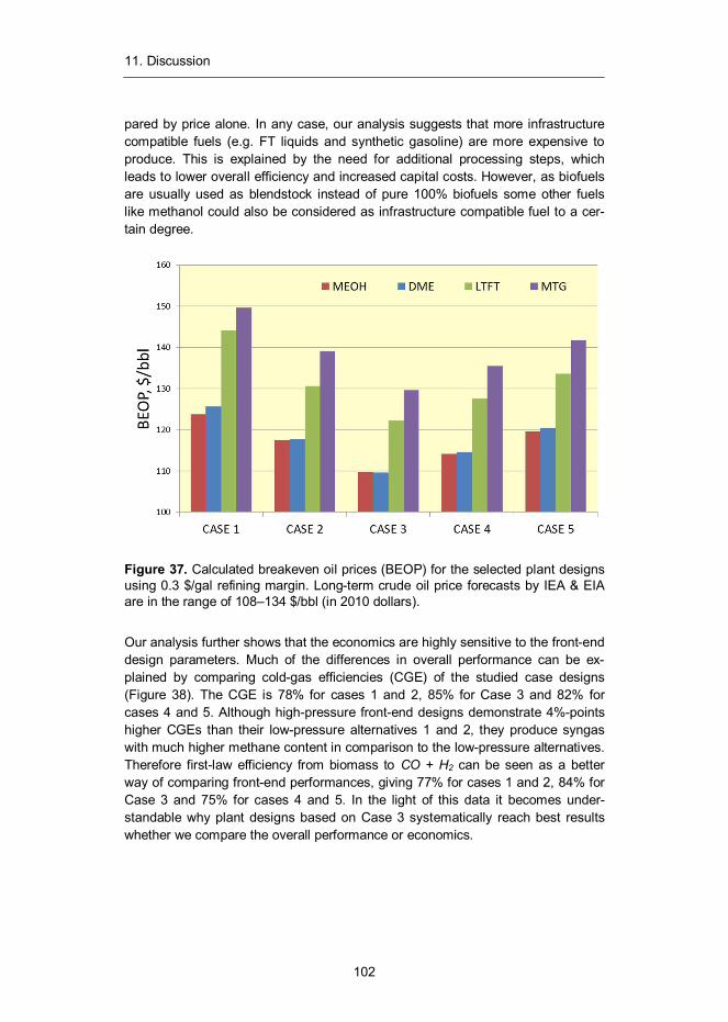
11. Discussion
102
pared by price alone. In any case, our analysis suggests that more infrastructure compatible fuels (e.g. FT liquids and synthetic gasoline) are more expensive to produce. This is explained by the need for additional processing steps, which leads to lower overall efficiency and increased capital costs. However, as biofuels are usually used as blendstock instead of pure 100% biofuels some other fuels like methanol could also be considered as infrastructure compatible fuel to a cer-tain degree.
Figure 37. Calculated breakeven oil prices (BEOP) for the selected plant designs using 0.3 $/gal refining margin. Long-term crude oil price forecasts by IEA & EIA are in the range of 108–134 $/bbl (in 2010 dollars).
Our analysis further shows that the economics are highly sensitive to the front-end design parameters. Much of the differences in overall performance can be ex-plained by comparing cold-gas efficiencies (CGE) of the studied case designs (Figure 38). The CGE is 78% for cases 1 and 2, 85% for Case 3 and 82% for cases 4 and 5. Although high-pressure front-end designs demonstrate 4%-points higher CGEs than their low-pressure alternatives 1 and 2, they produce syngas with much higher methane content in comparison to the low-pressure alternatives. Therefore first-law efficiency from biomass to CO + H2 can be seen as a better way of comparing front-end performances, giving 77% for cases 1 and 2, 84% for Case 3 and 75% for cases 4 and 5. In the light of this data it becomes under-standable why plant designs based on Case 3 systematically reach best results whether we compare the overall performance or economics.
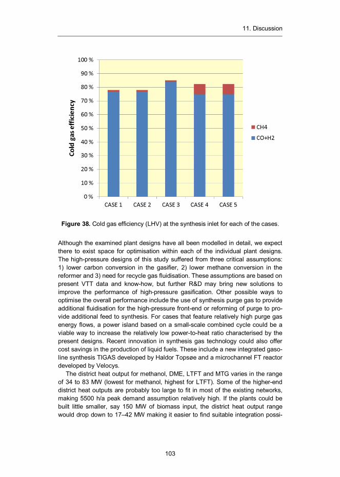
11. Discussion
103
Figure 38. Cold gas efficiency (LHV) at the synthesis inlet for each of the cases.
Although the examined plant designs have all been modelled in detail, we expect there to exist space for optimisation within each of the individual plant designs. The high-pressure designs of this study suffered from three critical assumptions: 1) lower carbon conversion in the gasifier, 2) lower methane conversion in the reformer and 3) need for recycle gas fluidisation. These assumptions are based on present VTT data and know-how, but further R&D may bring new solutions to improve the performance of high-pressure gasification. Other possible ways to optimise the overall performance include the use of synthesis purge gas to provide additional fluidisation for the high-pressure front-end or reforming of purge to pro-vide additional feed to synthesis. For cases that feature relatively high purge gas energy flows, a power island based on a small-scale combined cycle could be a viable way to increase the relatively low power-to-heat ratio characterised by the present designs. Recent innovation in synthesis gas technology could also offer cost savings in the production of liquid fuels. These include a new integrated gaso-line synthesis TIGAS developed by Haldor Topsøe and a microchannel FT reactor developed by Velocys.
The district heat output for methanol, DME, LTFT and MTG varies in the range of 34 to 83 MW (lowest for methanol, highest for LTFT). Some of the higher-end district heat outputs are probably too large to fit in most of the existing networks, making 5500 h/a peak demand assumption relatively high. If the plants could be built little smaller, say 150 MW of biomass input, the district heat output range would drop down to 17–42 MW making it easier to find suitable integration possi-
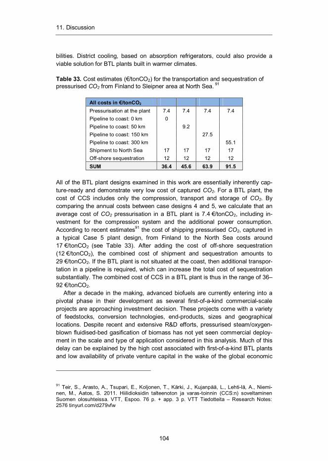
11. Discussion
104
bilities. District cooling, based on absorption refrigerators, could also provide a viable solution for BTL plants built in warmer climates.
Table 33. Cost estimates (€/tonCO2) for the transportation and sequestration of pressurised CO2 from Finland to Sleipner area at North Sea. 91
All costs in €/tonCO2 Pressurisation at the plant 7.4 7.4 7.4 7.4 Pipeline to coast: 0 km 0 Pipeline to coast: 50 km 9.2 Pipeline to coast: 150 km 27.5 Pipeline to coast: 300 km 55.1 Shipment to North Sea 17 17 17 17 Off-shore sequestration 12 12 12 12 SUM 36.4 45.6 63.9 91.5
All of the BTL plant designs examined in this work are essentially inherently cap-ture-ready and demonstrate very low cost of captured CO2. For a BTL plant, the cost of CCS includes only the compression, transport and storage of CO2. By comparing the annual costs between case designs 4 and 5, we calculate that an average cost of CO2 pressurisation in a BTL plant is 7.4 €/tonCO2, including in-vestment for the compression system and the additional power consumption. According to recent estimates91 the cost of shipping pressurised CO2, captured in a typical Case 5 plant design, from Finland to the North Sea costs around 17 €/tonCO2 (see Table 33). After adding the cost of off-shore sequestration (12 €/tonCO2), the combined cost of shipment and sequestration amounts to 29 €/tonCO2. If the BTL plant is not situated at the coast, then additional transpor-tation in a pipeline is required, which can increase the total cost of sequestration substantially. The combined cost of CCS in a BTL plant is thus in the range of 36– 92 €/tonCO2.
After a decade in the making, advanced biofuels are currently entering into a pivotal phase in their development as several first-of-a-kind commercial-scale projects are approaching investment decision. These projects come with a variety of feedstocks, conversion technologies, end-products, sizes and geographical locations. Despite recent and extensive R&D efforts, pressurised steam/oxygen-blown fluidised-bed gasification of biomass has not yet seen commercial deploy-ment in the scale and type of application considered in this analysis. Much of this delay can be explained by the high cost associated with first-of-a-kind BTL plants and low availability of private venture capital in the wake of the global economic
91 Teir, S., Arasto, A., Tsupari, E., Koljonen, T., Kärki, J., Kujanpää, L., Lehti-lä, A., Niemi-nen, M., Aatos, S. 2011. Hiilidioksidin talteenoton ja varas-toinnin (CCS:n) soveltaminen Suomen olosuhteissa. VTT, Espoo. 76 p. + app. 3 p. VTT Tiedotteita – Research Notes: 2576 tinyurl.com/d279vfw

11. Discussion
105
crisis. In any case, the present record-high price of crude oil together with long-term price forecasts reaching 120–130 $/bbl is likely to keep this technology at-tractive also in the future. However, for the world to remain on track with its mis-sion to restrict global warming to 2 °C, a significant amount of advanced BTL technologies are probably needed to be demonstrated before 2020. Regulatory actions and significant public support are therefore needed for the first plants to realise in time.
106
Acknowledgements We want to express our gratitude for all the people involved in the making of this report. Special thanks go to Drs. Eric Larson, Tom Kreutz and Bob Williams of Princeton University for their valuable comments and discussions that took place during a 12 month research visit to the Energy Systems Analysis Group. We would also like to thank Andras Horvath of Carbona-Andritz and Reijo Kallio of ÅF-Consult for sharing their expertise on steam system design issues and Dr. John Hansen of Haldor Topsøe for his comments on issues concerning general synthe-sis design. We would also like to thank Dr. Yrjö Solantausta of VTT for his valua-ble guidance and advice in economic analysis concerning chemical engineering and power plants.
107
References
1. Le Quéré, C., Andres, R. J., Boden, T., Conway, T., Houghton, R. A., House, J. I., Marland, G., Peters, G. P., van der Werf, G., Ahlström, A., Andrew, R. M., Bopp, L., Canadell, J. G., Ciais, P., Doney, S. C., Enright, C., Friedlingstein, P., Huntingford, C., Jain, A. K., Jourdain, C., Kato, E., Keeling, R., Levis, S., Levy, P., Lomas, M., Poulter, B., Raupach, M. R., Schwinger, J., Sitch, S., Stocker, B. D., Viovy, N., Zaehle, S., and Zeng, N. (2012) The global carbon budget 1959–2011. Earth System Science Data-Discussions (manuscript under review) 5: 1107–1157.
2. Peters, G., Andrew, R., Boden, T., Canadell, J., Ciais, P., Le Quéré, C. Marland, M., Raupach, M., Wilson, C. 2012. The challenge to keep global warming below two degrees. Nature Climate Change.
3. IEA statistics. 2012. CO2 Emissions from fuel combustion, highlights, In-ternational Energy Agency, tinyurl.com/6vz25nl
4. Transport, Energy and CO2: Moving toward Sustainability. 2009. Interna-tional Energy Agency, ISBN: 978-92-64-07316-6, tinyurl.com/3td6vso
5. Technology Roadmap: Biofuels for Transport. 2011. International Energy Agency, Paris, France.
6. Global Carbon Project. 2012. Carbon budget and trends 2012, ti-nyurl.com/aqdj65k, released on 3 December 2012.
7. Medium Term Oil and Gas Markets 2010. OECD/IEA, Paris.
8. Biofuels Mandates Around the World, Biofuels Digest website, published July 21st, 2011, tinyurl.com/blzy5a4
9. State of the Advanced Biofuels Industry, 2012: The Digest Primer, Biofu-els Digest website, published in March 14th, 2012, tinyurl.com/c9g975k
10. Molchanov, P. 2011. Gen2 Biofuels: Despite Growing Pains, Billion-Gallon Milestone Within Reach, Raymond James, Industry Brief.
11. International Energy Outlook. 2011. United States Energy Information Administration.
12. World Energy Outlook. 2011. International Energy Agency.
108
13. Hannula, I., Kurkela, E. 2012. A parametric modelling study for pressur-ised steam/O2-blown fluidised-bed gasification of wood with catalytic re-forming, Biomass and Bioenergy, Vol. 38, pp. 58–67, ISSN 0961-9534, A post-print is available via: tinyurl.com/c6tcqzq
14. McKeough, P., Kurkela, E. 2008. Process evaluations and design studies in the UCG project 2004–2007. Espoo, VTT. 45 p. VTT Tiedotteita - Re-search Notes; 2434. ISBN 978-951-38-7209-0; tinyurl.com/bre4cdx
15. Kurkela, E. 1996. Formation and removal of biomass-derived conta-minants in fluidized-bed gasification processes VTT Publications, Vol. 287. VTT Technical Research Centre of Finland.
16. Simell, P. 1997. Catalytic hot gas cleaning of gasification gas. Ph.D. the-sis, Helsinki University of Technology, TKK.
17. Kurkela, E., Simell, P., McKeough, P., Kurkela, M. 2008. Synteesikaasun ja puhtaan polttokaasun valmistus. Espoo, VTT. 54 p. + app. 5 s. VTT Publications; 682, ISBN 978-951-38-7097-3; tinyurl.com/cop4y83
18. Kurkela, E., Moilanen, A. & Kangasmaa, K. 2003. Gasification of biomass in a fluidised bed containing anti-agglomerating bed material. European Patent Office, Bulletin 2003/41. 10 p. WO 00/011115
19. Andritz Group, Company website, December 20th 2012, ti-nyurl.com/csm4p53
20. Kurkela, E., Ståhlberg, P., Laatikainen, J., Simell, P. 1993. Development of simplified IGCC processes for biofuels – supporting gasification re-search at VTT. Bioresource Technology, Vol. 46, 1–2, pp. 37–48.
21. Simell, P., Kurkela, E. 2007. Method for the purification of gasification gas. Pat. EP1404785 B1, publication date 3 Jan. 2007, application number EP2002743308A, application date 20 June 2002, priority EP2002743308A.
22. Kaltner, W. Personal communication, Clariant / Süd-Chemie AG, July 9th, 2012.
23. Supp, E. 1990. How to produce methanol from coal. Springer-Verlag Ber-lin, Heidelberg.
24. Hochgesand, G. 1970. Rectisol and Purisol. Ind. Eng. Chem., 62 (7), 37–43.
109
25. Weiss, H. 1988. Rectisol wash for purification of partial oxidation gases. Gas Sep. Pur. 2 (4), 171–176.
26. Fagernäs, L., Brammer, J. Wilen, C., Lauer, M., Verhoeff, F. 2010. Drying of biomass for second generation synfuel production, Biomass and Bioen-ergy, Vol. 34(9), pp. 1267–1277, ISSN 0961-9534, 10.1016/j.biombioe. 2010.04.005.
27. Wilen, C., Moilanen, A., Kurkela, E. 1996. Biomass feedstock analyses, VTT Publications 282, ISBN 951-38-4940-6
28. Metso broschure on KUVO belt dryer: tinyurl.com/cf5dyhv
29. Carbona Inc. 2009. BiGPower D71 Finnish case study report, Project co-founded by the European Commission within the Sixth Framework Pro-gramme, project no. 019761.
30. Smith, A.R., Klosek, J. 2001. A review of air separation technologies and their integration with energy conversion processes, Fuel Processing Technology, Vol. 70(2), pp. 115–134, ISSN 0378-3820.
31. Rackley, S. A. 2010. Carbon Capture and Storage. Elsevier.
32. IEA Greenhouse Gas R&D programme (IEA GHG). 2009. Biomass CCS Study, 2009/9.
33. Deliverable 4.9. European best practice guidelines for assessment of CO2 capture technologies. Project no: 213206. Project acronym: CAESAR. Project full title: Carbon-free Electricity by SEWGS: Advanced materials, Reactor-, and process design. FP7 – ENERGY.2007.5.1.1.
34. Kurkela, E., Koljonen, J. 1990. Experiences in the operation of the HTW process at the peat ammonia plant of Kemira Oy. VTT Symposium 107. Low grade fuels. Helsinki, 12–16 June 1989. Korhonen, Maija (ed.). Vol. 1, pp. 361–372.
35. Cran, J. 1981. Improved factored method gives better preliminary cost es-timates, Chem Eng, April 6.
36. Larson, E.D., Jin, H., Celik, F.E. 2009. Large-scale gasification-based coproduction of fuels and electricity from switchgrass, Biofuels, Biorprod. Bioref. 3:174–194.
37. Horvath, A. 2012. Personal communication.
110
38. Chemical Engineering. 2012. Vol. 119(4), ABI/INFORM Complete, p. 84, www.che.com/pci
39. Liu, G., Larson, E.D., Williams, R.H., Kreutz, T.G., Guoa, X. 2011. Online Supporting Material for Making Fischer-Tropsch Fuels and Electricity from Coal and Biomass: Performance and Cost Analysis, Energy & Fuels 25 (1).
40. Larson, E.D., Williams, R.H., Kreutz, T.G., Hannula, I., Lanzini, A. and Liu, G. 2012. Energy, Environmental, and Economic Analyses of Design Con-cepts for the Co-Production of Fuels and Chemicals with Electricity via Co-Gasification of Coal and Biomass, final report under contract DE-FE0005373 to The National Energy Technology Laboratory, US Depart-ment of Energy.
41. Laitila, J., Leinonen, A., Flyktman, M., Virkkunen, M. & Asikainen, A. 2010. Metsähakkeen hankinta- ja toimituslogistiikan haasteet ja kehittämistar-peet. VTT, Espoo. 143 p. VTT Tiedotteita – Research Notes: 2564 ISBN 978-951-38-7677-7 (nid.); 978-951-38-7678-4
42. Ott, J., Gronemann, V., Pontzen, F., Fiedler, E., Grossmann, G., Kerse-bohm, D., Weiss, G., Witte, C., Methanol. 2012. In Ullmann's Encyclope-dia of Industrial Chemistry, Wiley-VCH Verlag GmbH & Co. KgaA.
43. Patart, M. 1921. French patent, 540 343.
44. Tijm, P.J.A, Waller, G.J., Brown, D.M. 2001. Methanol technology devel-opments for the new millennium, Applied Catalysis A: General, Vol. 221(1–2), pp. 275–282, ISSN 0926-860X.
45. Appl, M. 1997. Ammonia, Methanol, Hydrogen, Carbon Monoxide – Mod-ern Production Technologies, Nitrogen, ISBN 1-873387-26-1.
46. Mansfield, K. 1996. ICI experience in methanol. Nitrogen (221), 27.
47. Lange, J., Methanol synthesis: a short review of technology improve-ments, Catalysis Today, Vol. 64(1–2), pp. 3–8, ISSN 0920-5861.
48. Hansen, J.B. 1997. Methanol Synthesis. In: Ertl, G., Knözinger, H., Weitkamp, J., Handbook of Heterogeneous Catalysis, Vol. 4, VCH, Wein-heim, p. 1856.
49. Converter options for methanol synthesis. 1994. Nitrogen (210), 36–44.
111
50. Katofsky, R. 1993. The production of fluid fuels from biomass, CEES Rpt 279, Center for Energy and Environmental Studies, Princeton University.
51. Biedermann, P., Grube, T., Hoehlein, B. (eds.). 2003. Methanol as an En-ergy Carrier. Schriften des Forschungszentrums Julich, Vol. 55, Julich.
52. Dimethyl ether. 2012. In Wikipedia, The Free Encyclopedia. Retrieved 11:04, July 26, 2012, from tinyurl.com/cnl25t5
53. Semelsberger, T., Borup, R. and Greene, H. 2006. Dimethyl ether (DME) as an alternative fuel, Journal of Power Sources, Vol. 156(2), pp. 497–511.
54. Navqi, S. 2002. Dimethyl ether as alternative fuel, Report No. 245, SRI Consulting, Menlo Park, CA.
55. Voss, B., Joensen, F. and Hansen, J. 1996. Preparation of fuel grade di-methyl ether. Granted patent, EP 0871602 B1.
56. Haugaard, J. and Voss, B. 2000. Process for the synthesis of a metha-nol/dimethyl ether mixture from synthesis gas. Granted patent, US 6191175.
57. Fleisch, T., McCarthy, C, Basu, A., Udovich, C., Charbonneau, P., Slodowske, Mikkelsen, S.E., McCandless, D. 1995. A New Clean Diesel Technology, Int. Congr. & Expos., Detroit, Michigan, Feb. 27–March 2, 1995.
58. Kreutz, T.G., Larson, E.D., Williams, R.H., Liu, G. 2008. Fischer-Tropsch Fuels from Coal and Biomass. In Proceedings of the 25th Annual Interna-tional Pittsburgh Coal Conference, Pittsburgh, PA.
59. Guangjian, L., Eric, D. Larson, R.H., Williams, T.G. Kreutz, and Guo, X. 2011. Making Fischer Tropsch Fuels and Electricity from Coal and Bio-mass: Performance and Cost Analysis Energy & Fuels 25 (1), pp. 415-437.
60. Van Bibber, L., Shuster, E., Haslbeck, J., Rutkowski, M., Olsen, S., Kra-mer, S. 2007. Baseline Technical and Economic Assessment of a Com-mercial Scale Fischer-Tropsch Liquids Facility; DOE/NETL-2007/1260; National Energy Technology Laboratory: Pittsburgh.
61. Hamelinck, C., Faaij, A., den Uil, H., Boerrigter, H. 2004. Production of FT transportation fuels from biomass; technical options, process analysis and
112
optimisation, and development potential, Energy, Vol. 29(11), pp. 1743–1771, ISSN 0360-5442.
62. McKeough, P. and Kurkela, E. 2008. Process evaluations and design studies in the UCG project 2004–2007, VTT Research notes 2434, Espoo Finland. tinyurl.com/bre4cdx
63. Fischer, F., Tropsch, H. Uber die Herstellung synthetischer ¨olgemische (Synthol) durch Aufbau aus Kohlenoxyd und Wasserstoff, Brennst. Chem. 4 (1923), pp. 276–285.
64. Fischer, F., Tropsch, H. German Patent 484337 1925.
65. Sie, S.T., Krishna, R. 1999. Fundamentals and selection of advanced Fischer–Tropsch reactors, Applied Catalysis A: General, Vol. 186(1–2), pp. 55–70.
66. Fischer-Tropsch (FT) Synthesis, NETL website, accessed July 23rd 2012, http://tinyurl.com/bvoumbw
67. de Klerk, A. 2011. Fischer-Tropsch refining, Wiley-VCH, 642 p. ISBN 9783527326051.
68. Sie, S.T., Senden, M.M.G., Van Wechem, H.M.H. 1991. Conversion of natural gas to transportation fuels via the shell middle distillate synthesis process (SMDS), Catalysis Today, Vol. 8(3), pp. 371–394, ISSN 0920-5861.
69. Anderson, R.B. 1961. Kinetics and reaction mechanism of the Fischer-Tropsch Synthesis In: Catalysis, ed. P.H. Emmett, 2nd edn. (Reinhold, New York, 1961), Vol. IV, p. 350.
70. Eilers, J., Posthuma, S.A., Sie, S.T. 1990/1991. The shell middle distillate synthesis process (SMDS), Catalysis Letters, Vol. 7(1–4), pp. 253–269.
71. Dry, M. 1981. In: Anderson, J., Boudart, M. (eds.). Catalysis Science and Technology, Vol. 1, Springer, Berlin, pp. 160–253.
72. Schulz, H. 1999. Short history and present trends of Fischer–Tropsch syn-thesis. Applied Catalysis A: General, Vol. 186(1–2), pp. 3–12, ISSN 0926-860X.
73. Anderson, R. In: Emmett, P. (ed), Catalysis, Vol. IV, Reinhold, 1956, Chap-ters 1–3.
113
74. Mark, E. 1996. Dry, Practical and theoretical aspects of the catalytic Fischer-Tropsch process, Applied Catalysis A: General, Vol. 138(2), pp. 319–344, ISSN 0926-860X.
75. Sie, S. 1998. Process development and scale up: IV. Case history of the development of a Fischer-Tropsch synthesis process, Reviews in Chemi-cal Engineering, Vol.14, No.2, pp. 109–157.
76. Moodley, D., Van de Loosdrecht, J., Saib, A. and Niemantsverdriet, J. 2009. In: Advances in Fischer-Tropsch Synthesis, Catalyst and Catalysis (eds Davis, B. and Occelli, M.), Taylor & Francis, Boca Raton, pp. 49–81.
77. Schulz, H., Claeys, M., Harms, S. Effect of water partial pressure on steady state Fischer-Tropsch activity and selectivity of a promoted cobalt catalyst, In: M. de Pontes, R.L. Espinoza, C.P. Nicolaides, J.H. Scholtz and M.S. Scurrell, Edit
78. Dry, M.E. 2002. The Fischer–Tropsch process: 1950–2000, Catalysis To-day, Vol. 71(3–4), pp. 227–241.
79. Schrauwen, F.J.M. 2004. In: Handbook of Petroleum Refining Processes (ed. R.A. Meyers), 3rd edn, McGraw-Hill, New York, pp. 15.25–15.40.
80. Smith, R. and Asaro, M. 2005. Fuels of the Future. Technology Intelli-gence for Gas to Liquids Strategies, Stanford Research Institute, Menlo Park, CA.
81. van der Laan, G., Beenackers, T. 2000. Kinetics, selectivity and scale p of the Fischer-Tropsch synthesis. NPT Procestechnologie 2000(3), pp. 8–21.
82. Sullivan, R.F. and Scott, J.W. 1983. The Development of Hydrocracking, Heterogeneous Catalysis, Vol. 222, Chapter 24, pp. 293–313, ACS Sym-posium Series.
83. Kobolakis, I. and Wojciechowski, B.W. 1985. The catalytic cracking of a fischer-tropsch synthesis product, The Canadian Journal of Chemical En-gineering, Vol. 63(2). pp. 269–277.
84. Wiley Critical Content – Petroleum Technology. 2007. Vol. 1–2. John Wiley & Sons.
85. Chang, C.D. 1992. The New Zealand Gas-to-Gasoline plant: An engineer-ing tour de force, Catalysis Today, Vol.13(1), pp. 103–111.
114
86. Wittcoff, H.A., Reuben, B.G., Plotkin, J.S. 2004. Industrial Organic Chemi-cals (2nd Edition). John Wiley & Sons.
87. Gasoline – TIGAS, Haldor Topsøe website. Accessed July 30th, 2012. ti-nyurl.com/bqdmr95
88. Rostrup-Nielsen, T., Højlund Nielsen, P.E., Joensen, F., Madsen. J. Pol-ygeneration – Integration of Gasoline Synthesis and IGCC Power Produc-tion Using Topsoe’s TIGAS Process. tinyurl.com/b6wr3kg
89. Kam, A.Y. Schreiner, M., Yurchak, S. 1984. Mobil Methanol-to-Gasoline Process,” chapter 2–3 in Handbook of Synfuels Technology, R.A. Meyers (ed.), McGraw-Hill.
90. Larson, E.D., Williams, R.H., Kreutz, T.G., Hannula, I., Lanzini, A. and Liu, G. 2012. Appendix B – Process Design and Analysis for Co-Production of Electricity and Synthetic Gasoline via Co-Gasification of coal and Biomass with CCS” final report under contract DE-FE0005373 to The National En-ergy Technology Laboratory, US Department of Energy.
91. Teir, S., Arasto, A., Tsupari, E., Koljonen, T., Kärki, J., Kujanpää, L., Lehti-lä, A., Nieminen, M., Aatos, S. 2011. Hiilidioksidin talteenoton ja varas-toinnin (CCS:n) soveltaminen Suomen olosuhteissa. VTT, Espoo. 76 p. + app. 3 s. VTT Tiedotteita – Research Notes: 2576 tinyurl.com/d279vfw
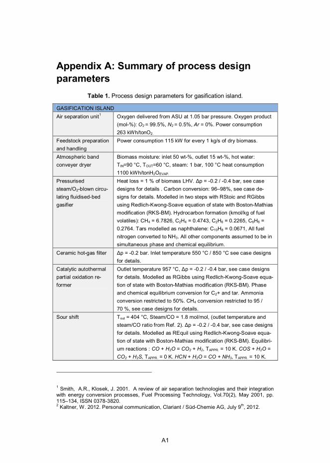
A1
Appendix A: Summary of process design parameters
Table 1. Process design parameters for gasification island.
GASIFICATION ISLAND Air separation unit1 Oxygen delivered from ASU at 1.05 bar pressure. Oxygen product
(mol-%): O2 = 99.5%, N2 = 0.5%, Ar = 0%. Power consumption 263 kWh/tonO2.
Feedstock preparation and handling
Power consumption 115 kW for every 1 kg/s of dry biomass.
Atmospheric band conveyer dryer
Biomass moisture: inlet 50 wt-%, outlet 15 wt-%, hot water: TIN=90 °C, TOUT=60 °C, steam: 1 bar, 100 °C heat consumption 1100 kWh/tonH2OEVAP.
Pressurised steam/O2-blown circu-lating fluidised-bed gasifier
Heat loss = 1 % of biomass LHV. p = -0.2 / -0.4 bar, see case designs for details . Carbon conversion: 96–98%, see case de-signs for details. Modelled in two steps with RStoic and RGibbs using Redlich-Kwong-Soave equation of state with Boston-Mathias modification (RKS-BM). Hydrocarbon formation (kmol/kg of fuel volatiles): CH4 = 6.7826, C2H4 = 0.4743, C2H6 = 0.2265, C6H6 = 0.2764. Tars modelled as naphthalene: C10H8 = 0.0671, All fuel nitrogen converted to NH3. All other components assumed to be in simultaneous phase and chemical equilibrium.
Ceramic hot-gas filter p = -0.2 bar. Inlet temperature 550 °C / 850 °C see case designs for details.
Catalytic autothermal partial oxidation re-former
Outlet temperature 957 °C, p = -0.2 / -0.4 bar, see case designs for details. Modelled as RGibbs using Redlich-Kwong-Soave equa-tion of state with Boston-Mathias modification (RKS-BM). Phase and chemical equilibrium conversion for C2+ and tar. Ammonia conversion restricted to 50%. CH4 conversion restricted to 95 / 70 %, see case designs for details.
Sour shift Tout = 404 °C, Steam/CO = 1.8 mol/mol, (outlet temperature and steam/CO ratio from Ref. 2). p = -0.2 / -0.4 bar, see case designs for details. Modelled as REquil using Redlich-Kwong-Soave equa-tion of state with Boston-Mathias modification (RKS-BM). Equilibri-um reactions : CO + H2O = CO2 + H2, TAPPR. = 10 K. COS + H2O = CO2 + H2S, TAPPR. = 0 K. HCN + H2O = CO + NH3, TAPPR. = 10 K.
1 Smith, A.R., Klosek, J. 2001. A review of air separation technologies and their integration with energy conversion processes, Fuel Processing Technology, Vol.70(2), May 2001, pp. 115–134, ISSN 0378-3820. 2 Kaltner, W. 2012. Personal communication, Clariant / Süd-Chemie AG, July 9th, 2012.
A2
Scrubber Scrubbing liquid: water. TINLET 220 °C. Two-step cooling: T1OUT=
60 °C, T2OUT= 30 °C. Complete ammonia removal.
Rectisol acid gas removal3
100 % H2S capture, CO2 capture level see case designs for de-tails. Utilities: Electricity (other than for refrigeration) = 1900 kJ/kmol(CO2+H2S); Refrigeration 3 x duty needed to cause -12 K temperature change in the syngas; 5 bar steam = 6.97 kg/kmol (H2S+CO2)
Heat exchangers3 p/p = 2%; TMIN = 15°C (gas-liq), 30 °C (gas-gas). Heat loss = 1% of heat transferred
Table 2. Process design parameters for auxiliary equipment.
AUXILIARY EQUIPMENT Auxiliary boiler Modelled as RStoic, p = - 0.1 bar, Lambda = 1.20, Air preheat to
250 °C with fluegas Heat recovery & Steam system4,5
Flue gas TOUT=150 °C, feed water pressure 100 bar, superheater p = -6 bar, stream drum blowdowns: 2% of inlet flow, Deaerator
TOUT = 120 °C, Steam turbine4,6 Inlet steam parameters: 94 bar, 500 °C; Extraction steam parame-
ters: HP = 30 bar, 353 °C; IP = see case designs for details; LP = 5 bar, 178 °C; ISENTROPIC = 0.78, GENERATOR=0.97 , mechanical=0.98 (generator and mechanical efficiency from Ref. 7)
Compressors8 Stage pressure ratio <2, POLYTROPIC= 0.85, DRIVER= 0.92, MECHANI-
CAL= 0.98 Multistage compres-sors (>4.5 kg/s)9
Stage pressure ratio <2, POLYTROPIC= 0.87 , DRIVER= 0.92, MECHAN-
ICAL= 0.98, TINTERCOOLER= 35 °C, p/pINTERCOOLER= 1% Multistage compres-sors (<4.5 kg/s)9
Stage pressure ratio <2, POLYTROPIC= 0.85, DRIVER= 0.90, MECHANICAL= 0.98, TINTERCOOLER= 35 °C, p/pINTERCOOLER= 1 %
Pumps8 HYDRAULIC = 0.75, DRIVER = 0.90,
3 Liu, G., Larson, E.D., Williams, R.H., Kreutz, T.G., Guoa, X. 2011. Online Supporting Mate-rial for Making Fischer-Tropsch Fuels and Electricity from Coal and Biomass: Performance and Cost Analysis, Energy & Fuels 25 (1). 4 Horvath, A. 2012. Personal communication, Carbona-Andritz, May 15th 2012. 5 McKeough, P. 2011. Personal communication, Andritz, September 2011. 6 Kallio, R. 2012. Personal communication, ÅF-consulting, October 2012. 7 Phillips et al. 2007. Thermochemical Ethanol via Indirect Gasification and Mixed Alcohol Synthesis of Lignocellulosic Biomass Technical Report NREL/TP-510-41168. 8 Chiesa, P., Consonni, S., Kreutz, T., Williams, R. 2005. Co-production of hydrogen, elec-tricity and CO2 from coal with commercially ready technology. Part A: Performance and emissions, International Journal of Hydrogen Energy, Vol. 30(7), pp. 747–767. 9 Glassman, A.J. 1992. Users Manual for Updated Computer Code for Axial-Flow Compres-sor Conceptual Design. University of Toledo, Toledo, Ohio.
A3
Table 3. Process design parameters for synthesis islands.
SYNTHESIS ISLANDS Low-pressure met-hanol
TREACTION= 260 °C, PMAKE-UP= 80 bar, p =-5 bar, Modelled as REquil using Soave-Redlich-Kwong equation of state (SRK). Equilibrium reactions: CO + 2H2 = CH4O, TAPPR. = 10 K; CO2 + 3H2 = CH4O + H2O, TAPPR. = 10 K.
Single-step DME10 T1IN= 240 °C, T3
OUT = 280 °C, PMAKE-UP= 60 bar, p =-1.4 bar, Modelled as three separate REquil reactors with intercooling to 240 °C using Soave-Redlich-Kwong equation of state (SRK). Equilibrium reactions: CO + 2H2 = CH4O, TAPPR. = 10 K; 2CH4O = C2H6O + H2O, TAPPR. = 30 K; CO + H2O = CO2 + H2, TAPPR. = 10 K.
Low-temperature Fischer-Tropsch
TREACTION= 200 °C, PMAKE-UP= 30 bar, p =-5 bar, Modelled as REquil using Redlich-Kwong-Soave equation of state with Boston-Mathias modification (RKS-BM). 91% C5+ selectivity, 80 % per-pass conversion. 0.9 -value with C1-C4 fraction redistributed to 74 mol% C1, 16 mol% C2, 6 mol% C3 and 4 mol% C4 while input H2O, CO2, N2 as well as unreformed methane, ethane and longer hydrocarbons considered inert. Hydrocracker operated at 325 °C and 40 bar. Mass fraction of required hydrogen to hydrocracker feed = 1%, gas make from the process = 2%, Depending on the hydrocracking severity, yield ratios of naphtha, kerosene and gas oil can be varied from 15 25 60 (gas oil mode) to 25 50 25 (kerosene mode).
Methanol-to-Gasoline DME reactor: TIN= 297 °C, TOUT=407 °C, PIN= 23 bar, p =-1 bar, Modelled as REquil using Soave-Redlich-Kwong equation of state (SRK). Equilibrium reaction: 2CH4O = C2H6O + H2O, TAPPR. = 30 K. Gasoline reactor: TREACTOR= 400 °C, PIN= 22 bar, p =-1 bar, Modelled as REquil using Soave-Redlich-Kwong equation of state (SRK). See report for MTG reactor yield structure. Relative mass yields from 1 ton of raw product in the refining area are 880 kg of gasoline blendstock, 100 kg of LPG and 20 kg of purge gas.
10 Hansen, J. 2012. Personal communication, Haldor Topsoe, November 12th 2012.

A4
Series title and number VTT Technology 91
Title Liquid transportation fuels via large-scale fluidised-bed gasification of lignocellulosic biomass
Author(s) Ilkka Hannula & Esa Kurkela
Abstract With the objective of gaining a better understanding of the system design trade-offs and economics that pertain to biomass-to-liquids processes, 20 individual BTL plant designs were evaluated based on their technical and economic performance. The investigation was focused on gasification-based processes that enable the conversion of biomass to methanol, dimethyl ether, Fischer-Tropsch liquids or synthetic gasoline at a large (300 MWth of biomass) scale. The biomass conversion technology was based on pressurised steam/O2-blown fluidised-bed gasification, followed by hot-gas filtration and catalytic conversion of hydrocarbons and tars. This technology has seen extensive development and demonstration activities in Finland during the recent years and newly generated experi-mental data has also been used in our simulation models. Our study included conceptual design issues, process descriptions, mass and ener-gy balances and production cost estimates.
Several studies exist that discuss the overall efficiency and economics of biomass conversion to transportation liquids, but very few studies have presented a detailed comparison between various syntheses using con-sistent process designs and uniform cost database. In addition, no studies exist that examine and compare BTL plant designs using the same front-end configuration as described in this work.
Our analysis shows that it is possible to produce sustainable low-carbon fuels from lignocellulosic biomass with first-law efficiency in the range of 49.6–66.7% depending on the end-product and process condi-tions. Production cost estimates were calculated assuming Nth plant economics and without public investment support, CO2 credits or tax assumptions. They are 58–65 €/MWh for methanol, 58–66 €/MWh for DME, 64–75 €/MWh for Fischer-Tropsch liquids and 68–78 €/MWh for synthetic gasoline.
ISBN, ISSN ISBN 978-951-38-7978-5 (Soft back ed.) ISBN 978-951-38-7979-2 (URL: http://www.vtt.fi/publications/index.jsp) ISSN-L 2242-1211 ISSN 2242-1211 (Print) ISSN 2242-122X (Online)
Date April 2012
Language English, Finnish abstract
Pages 114 p. + app. 3 p.
Keywords Biomass, biofuels, gasification, methanol, DME, Fischer-Tropsch, MTG
Publisher VTT Technical Research Centre of Finland P.O. Box 1000, FI-02044 VTT, Finland, Tel. 020 722 111

Julkaisun sarja ja numero VTT Technology 91
Nimeke Liikenteen biopolttoaineiden valmistus metsätäh-teistä leijokerroskaasutuksen avulla
Tekijä(t) Ilkka Hannula & Esa Kurkela
Tiivistelmä Julkaisussa tarkastellaan metsätähteen kaasutukseen perustuvien liikenteen bio-polttoaineiden tuotantolaitosten toteutusvaihtoehtoja ja arvioidaan näiden vaikutuk-sia neljän eri lopputuotteen – metanoli, dimetyylieetteri (DME), Fischer-Tropsch-nesteet ja synteettinen bensiini (MTG) – kannalta. Arviointien perustaksi valittiin Suomessa viime vuosina kehitetty prosessi, joka perustuu paineistettuun leijuker-roskaasutukseen, kaasun kuumasuodatukseen sekä katalyyttiseen tervojen ja hiilivetyjen reformointiin. Kaasutusprosessin perusvaihtoehdossa puun kaasutus tapahtuu 5 barin paineessa, minkä jälkeen kaasuttimesta poistuva raakakaasu jäähdytetään 550 °C:n lämpötilaan ja suodatetaan ennen sen johtamista reforme-riin, jossa kaasun lämpötila jälleen nousee osittaispolton takia yli 900 °C:seen. Tämän perusprosessin toimivuus on demonstroitu VTT:llä vuosina 2007–2011 toteutetuissa pitkäkestoisissa PDU-kokoluokan koeajoissa sekä teollisella pilottilai-toksella. Tässä julkaisussa esitettyjen tarkastelujen kohteena oli kaikissa tapauk-sissa suurikokoinen tuotantolaitos, jonka metsätähteen käyttö vastasi saapumisti-lassaan 300 MW:n tehoa.
Julkaisun tulosten perusteella puumaisesta biomassasta on mahdollista tuottaa uusiutuvia biopolttonesteitä 50–67 %:n energiahyötysuhteella, lopputuotteesta ja prosessiolosuhteista riippuen. Korkein polttoaineen tuotannon hyötysuhde saavute-taan metanolin ja DME:n valmistuksessa. Mikäli myös sivutuotteena syntyvä läm-pöenergia pystytään hyödyntämään esimerkiksi kaukolämpönä, nousee biomassan käytön kokonaishyötysuhde 74–80 %:n tasolle. Parhaillaan kehitystyön kohteena oleva kaasun suodatuslämpötilan nosto perusprosessin 550 °C:sta 850 °C:seen parantaisi polttonesteen tuotannon hyötysuhdetta 5–6 prosenttiyksikköä.
Kaupalliseen teknologiaan perustuvien tuotantokustannusarvioiden laskentaole-tuksissa ei huomioitu julkista tukea, päästökauppahyötyjä tai verohelpotuksia. Eri prosessivaihtoehtojen tuotantokustannuksiksi arvioitiin 58–65 €/MWh metanolille, 58–66 €/MWh DME:lle, 64–75 €/MWh Fischer-Tropsch-nesteille ja 68–78 €/MWh synteettiselle polttonesteelle. Korkeimmat tuotantokustannukset ovat kaasutuspro-sessin perusvaihtoehdolle ja tapauksille, joissa sivutuotelämmölle ei ole muuta hyötykäyttöä kuin biomassan kuivaus ja lauhdesähkön tuotanto. Alhaisimmat kustannukset taas saavutetaan kaukolämpöintegroiduilla laitoksilla, joissa kaasun suodatus tapahtuu korkeassa lämpötilassa. Tuotteiden kustannusarviot ovat lähellä nykyisten raakaöljypohjaisten tuotteiden verotonta hintaa, eivätkä kaupalliset lai-tokset sen vuoksi vaatisi merkittäviä julkisia tukia tullakseen kannattaviksi. Sen sijaan ensimmäiset uraauurtavat tuotantolaitokset ovat oletettavasti merkittävästi tässä esitettyjä arvioita kalliimpia, minkä vuoksi teknologian kaupallistuminen edellyttää ensimmäisten laitosten osalta merkittävää julkista tukea.
ISBN, ISSN ISBN 978-951-38-7978-5 (nid.) ISBN 978-951-38-7979-2 (URL: http://www.vtt.fi/publications/index.jsp) ISSN-L 2242-1211 ISSN 2242-1211 (painettu) ISSN 2242-122X (verkkojulkaisu)
Julkaisuaika Huhtikuu 2013
Kieli Englanti, suomenkielinen tiivistelmä
Sivumäärä 114 s. + liitt. 3 s.
Avainsanat Biomass biofuels gasification methanol DME Fischer-Tropsch MTG
Julkaisija VTT PL 1000, 02044 VTT, Puh. 020 722 111

VTT Technical Research Centre of Finland is a globally networked multitechnological contract research organization. VTT provides high-end technology solutions, research and innovation services. We enhance our customers’ competitiveness, thereby creating prerequisites for society’s sustainable development, employment, and wellbeing.
Turnover: EUR 300 million Personnel: 3,200
VTT publications
VTT employees publish their research results in Finnish and foreign scientific journals, trade periodicals and publication series, in books, in conference papers, in patents and in VTT’s own publication series. The VTT publication series are VTT Visions, VTT Science, VTT Technology and VTT Research Highlights. About 100 high-quality scientific and profes-sional publications are released in these series each year. All the publications are released in electronic format and most of them also in print.
VTT VisionsThis series contains future visions and foresights on technological, societal and business topics that VTT considers important. It is aimed primarily at decision-makers and experts in companies and in public administration.
VTT ScienceThis series showcases VTT’s scientific expertise and features doctoral dissertations and other peer-reviewed publications. It is aimed primarily at researchers and the scientific community.
VTT TechnologyThis series features the outcomes of public research projects, technology and market reviews, literature reviews, manuals and papers from conferences organised by VTT. It is aimed at professionals, developers and practical users.
VTT Research HighlightsThis series presents summaries of recent research results, solutions and impacts in selected VTT research areas. Its target group consists of customers, decision-makers and collaborators.
VT
T T
EC
HN
OL
OG
Y 9
1
Liq
uid
tran
spo
rtatio
n fu
els via
larg
e-sc
ale
flu
idise
d-b
ed
ga
sificatio
n...
ISBN 978-951-38-7978-5 (soft back ed.)ISBN 978-951-38-7979-2 (URL: http://www.vtt.fi/publications/index.jsp)ISSN-L 2242-1211ISSN 2242-1211 (Print)ISSN 2242-122X (Online)
Liquid transportation fuels via large-scale fluidised-bed gasification of lignocellulosic biomass
With the objective of gaining a better understanding of the system design trade-offs and economics that pertain to biomass-to-liquids processes, 20 individual BTL plant designs were evaluated based on their technical and economic performance. The investigation was focused on gasification-based processes that enable the conversion of biomass to methanol, dimethyl ether, Fischer-Tropsch liquids or synthetic gasoline at a large (300 MWth of biomass) scale. The biomass conversion technology was based on pressurised steam/O2-blown fluidised-bed gasification, followed by hot-gas filtration and catalytic conversion of hydrocarbons and tars. This technology has seen extensive development and demonstration activities in Finland during the recent years and newly generated experimental data has been incorporated into the simulation models. Our study included conceptual design issues, process descriptions, mass and energy balances and production cost estimates.
Liquid transportation fuels via large-scale fluidised-bed gasification of lignocellulosic biomassIlkka Hannula | Esa Kurkela
•VISIONS•S
CIE
NC
E•T
ECHNOLOGY•R
ES
EA
RC
HHIGHLIGHTS
91