Retrospective Theses and Dissertations Iowa State University Capstones, Theses andDissertations

1964

Liquid-phase mass transfer at low flow rates in apacked columnJohn Earnest FrandoligIowa State University

Follow this and additional works at: https://lib.dr.iastate.edu/rtd

Part of the Chemical Engineering Commons

This Dissertation is brought to you for free and open access by the Iowa State University Capstones, Theses and Dissertations at Iowa State UniversityDigital Repository. It has been accepted for inclusion in Retrospective Theses and Dissertations by an authorized administrator of Iowa State UniversityDigital Repository. For more information, please contact digirep@iastate.edu.

Recommended CitationFrandolig, John Earnest, "Liquid-phase mass transfer at low flow rates in a packed column " (1964). Retrospective Theses andDissertations. 2985.https://lib.dr.iastate.edu/rtd/2985

This dissertation has been 64—9262 microfilmed exactly as received

FRANDOLIG, John Earnest, 1934-LIQUED—PHASE MASS TRANSFER AT LOW FLOW RATES IN A PACKED COLUMN.

Iowa State University of Science and Technology Ph.D., 1964 Engineering, chemical

University Microfilms, Inc., Ann Arbor, Michigan

LIQUID-PHASE MASS TRANSFER AT LOW FLOW RATES

IN A PACKED COLUMN

John Earnest Frandolig

A Dissertation Submitted to the

G-raduate Faculty in Partial Fulfillment of

The Requirements for the -Degree of

DOCTOR OF PHILOSOPHY

Major Subject: Chemical Engineering

Approved:

In Charge of Major Work

Head of Major Department

Iowa State University Of Science and Technology

Ames, Iowa

1964

Signature was redacted for privacy.

Signature was redacted for privacy.

Signature was redacted for privacy.

il

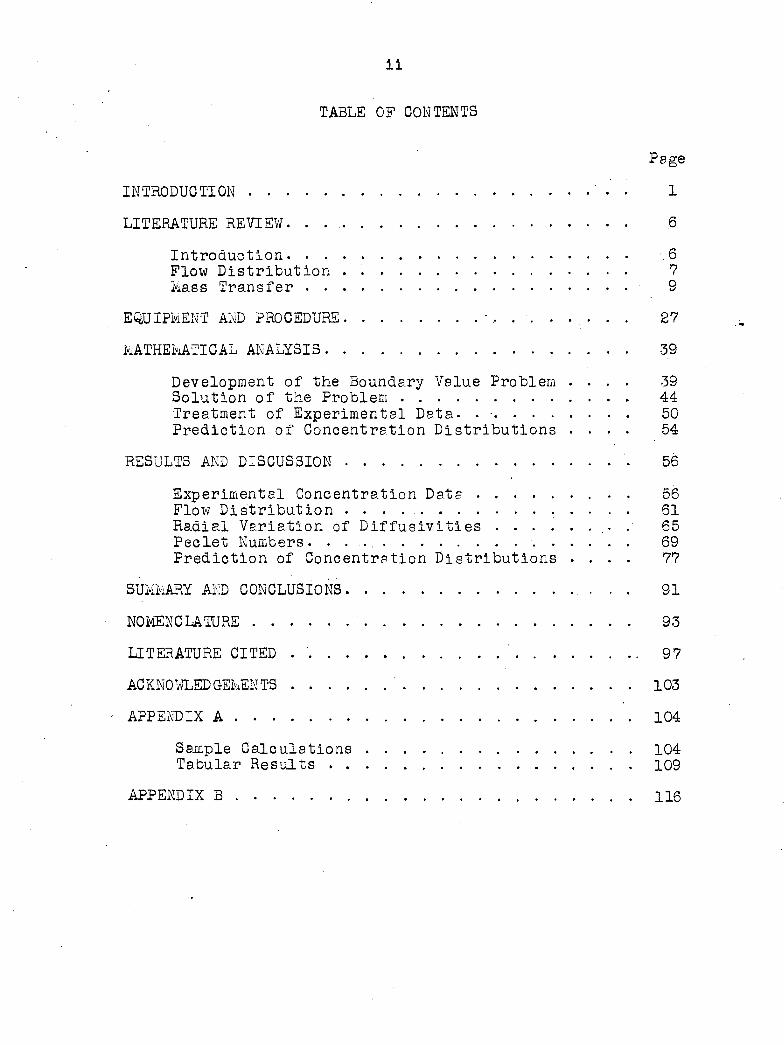
TABLE OF CONTENTS

Page

INTRODUCTION . . . . . 1

LITERATURE REVIEW. . . • .6

Introduction 6 Flow Distribution . 7 Mass Transfer 9

EQUIPMENT AND PROCEDURE ........ 27

MATHEMATICAL ANALYSIS. 39

Development of the Boundary Value Problem .... 39 Solution of the Problem .44 Treatment of Experimental Data- . • 50 Prediction of Concentration Distributions .... 54

RESULTS AND DISCUSSION ..... 56

Experimental Concentration Data 56 Flow Distribution . . . . 51 Radial Variation of Dif fusivities 65 Peclet Numbers. 69 Prediction of Concentration Distributions .... 77

SUMMARY AND CONCLUSIONS . . . 91

NOMENCLATURE 93

LITERATURE CITED 97

ACKNOWLEDGEMENTS 103

APPENDIX A 104

Sample Calculations 104 Tabular Results 109

APPENDIX B 116

1

INTRODUCTION

The successful application of any engineering design

technique depends not only on its scientific soundness but

also on the quality of the available quantitative descriptions

of the various component mechanisms making up the total pro­

cess. Probably the least understood mechanisms, and certainly

very key ones in process design work, are those associated

with heat, mass, and momentum transfer in fixed-bed systems.

In view of the population density of fixed-bed processes in

the chemical and allied industries (e.g., absorption and

adsorption processes, fixed-bed catalytic reactors, packed-

column distillation and extraction systems, and chromato­

graphic columns ), it follows that much attention should be

focused on the fundamental aspects of these transfer mechan­

isms. Present analogies, although incomplete, and possible

future ones between the heat, mass, and momentum transfer

processes make the study of any one essentially a study of

related aspects of the other two.

Mass. transport phenomena in cylindrical fixed-bed systems

have been studied primarily from two points of view. The

first and most generally accepted attack has been that of

mathematically characterizing the system by the conventional

overall mass transfer coefficient. This type of analysis has

been applied to two-phase unit operations such as liquid-

liquid extraction and gas-liquid absorption. The results of

2

these studies are generally applicable only to other identi­

cal systems; i.e., systems in which the chemical components,

the packing characteristics, and the flow rates are the same.

Furthermore, the correlation of dimensionless groups arising

from these studies has not been completely successful.

A second approach to the problem is that of considering

the mixing, stream-splitting, and molecular diffusion in a

binary mixture in a single phase. Studies of this type may be

further subdivided into two groups: l) that in which the

total transfer process is characterized by a single effective

axial dispersion coefficient (axial dispersivity), and 2) that

in which the mass transfer process is characterized by arbi­

trarily defined coefficients, each of which accounts for the

transfer in a given coordinate direction.

The axial dispersivity model has been used to describe

unsteady-state and frequency response systems in one spatial

dimension. Thus, the axial dispersivity accounts for the mass

transfer caused by the combined influence of the velocity pro­

file, molecular diffusion, and the mixing action generated by

the presence of the packing. Mathematically, this type of

system is described by a material balance around a cylindrical

element of the bed which is of differential length dz:

Dl iF§ ~v ir= irr (1) oz^ oz at

where C = concentration of transferring material

Dl = axial dispersivity

3

V = mean superficial velocity

z = axial coordinate

t = time.

Analytical solutions of this equation with various boundary

conditions imposed have previously been accomplished ( 15,

23, 33, 40, 41, 53, 54, 57). Results from this type of anal­

ysis are useful in certain simplified reactor designs and in

process dynamics studies.

The above two models for describing the mass transfer

process in fixed-bed systems have an inherent limitation:

the point values of the concentrations are not considered and

if the results are to b.e used for design purposes, point con­

centrations are not calculable. For a few problems this

limitation is not serious. However, in the design of cata­

lytic reactors in which the reaction rate depends on point

temperatures and concentrations, these models appear inade­

quate. The model in which the- mass transfer is characterized

by directional coefficients allows for the consideration of

point concentrations and thus is a more realistic approach to

the problem. The detailed mathematical treatment of this

model is given in a later section of this report.

In previous fixed-bed studies the axial transfer coeffi­

cient, hereinafter referred to as the axial diffusivity, was

not evaluated as such. The analysis of experimental concentra­

tion data has been restricted by one of two assumptions:

4

1) the axial cliffusivity was assumed equal to the radial

diffusivity, or 2) the axial mass transfer was assumed negli­

gible when compared to the bulk flow effect. Results from

axial dispersion,studies have indicated that both of these

assumptions may be invalid, especially in the design of cata­

lytic reactors and extraction systems.

The purpose of this work was twofold: l) to obtain exper­

imental concentration data suitable for comparison with future

theoretical predictions, and 2) to analyze these data in terms

of calculated effective axial and radial diffusivities and

Peclet numbers. Particular emphasis was placed on determin­

ing the effect of neglecting axial transfer on the prediction

of concentration profiles for a non-reactive liquid system.

The experimental work consisted of measuring radial con­

centration distributions for a dye being transported in a main

stream of water flowing slowly through a packed column. The

column was 3.97 inches in diameter and was packed with 0.262-

inch spherical particles. Data were obtained at four axial

levels above a centrally located injection tube for Reynolds

numbers between 7.1 and 84.9. Samples were removed from the

column by a specially designed probe assembly which "averaged11

the sample for a given radial position over a number of angu­

lar positions. The data are presented in dimensionless units

based on the measured steady-state mean concentration in the

column.

5

Analysis of the data was made in accordance with a solu­

tion of the boundary value problem set up to describe the

physical system.

6

LITERATURE REVIEW

Introduction

Most of the studies of mass transfer in flowing fluids

have been carried out primarily in three systems: l) coaxial

fluid streams in ducts, 2) wetted-wall columns, and 3) beds

of particles, both fixed and fluidized. The studies involving

the coaxial streams may be considered the most basic since,

in effect, all processes deal essentially with the flow of

fluids in interstices of one kind or another. However,

"extrapolation" of new knowledge of this system to the other

two is obviously quite dangerous because of the complexity

introduced by the two-phases on the one hand, and the particle

and packing characteristics on the other. Yet the study of

mass transfer in beds of particles has the closest practial

chemical engineering application of the three systems as evi­

denced by the numerous catalytic reactors, absorption columns,

chromatographic columns, packed distillation, extraction, and

other such towers found throughout the process industries. It

is perhaps for this reason that so much basic work has been

carried out in this system.

The literature concerning studies of mass, momentum, and

heat transfer processes is voluminous. Seagrave (52) presents

a quite complete review of mass transfer in coaxial fluid

streams in ducts and in wetted-wall columns. Herein is dis­

cussed only some of the more pertinent work in the field of

7

mass transfer as applied to fixed-bed systems. The choice of

particular papers covers the many far-ranging aspects of this

subject as applied to various unit operations, such as absorp­

tion, extraction, and chromatographic separation, and to cata­

lytic reactors.

Flow Distribution

Of prime importance in the study of any fixed-bed trans­

fer process is a knowledge of the distribution of flow across

the bed. Primarily because of the increased mathematical com­

plexity of considering a non-uniform flow distribution in

fixed-bed calculations, investigators have generally assumed

flat profiles in their work. Arthur et al. (4) first showed

qualitatively that this assumption is generally invalid.

Semi-quantitative results indicated that the flow rate was

greatest slightly removed from the containing wall.

Morales et. al. (42) and Schwartz and Smith (51), using

a hot-wire anemometer, studied this phenomenon at relatively

high flow rates for air flowing through beds of cylinders and

spheres. They found that the peak velocity occurred approxi­

mately one pellet diameter away from the column wall. For the

ratio of column diameter to pellet diameter less than 30 this

peak velocity ranged from 30 to 100 per cent greater than the

velocity at the center of the bed. The divergence of the pro­

file from the assumption of a uniform velocity was found to be

8

less than 20 per cent only for ratios of column diameter to

pellet diameter greater than 30.

The flow distribution may be explained, in part, by the

variation of void fraction in the bed. Schaffer (50) and

Roblee et al. (48) found that the void fraction in packed

cylindrical columns was essentially constant throughout the

center of the bed and increased as the wall was approached.

Dorweiler (21), using a hot-wire anemometer, determined

the flow distribution for air flowing through a 4.026-inch

i.d. column packed with 0.262-inch spherical particles. He

concluded that the hot-wire anemometer was sufficiently accu­

rate, on the basis of overall material balances, only for

mean superficial velocities above 0.2 foot per second. No

data have yet been reported for lower flow rates for either

gaseous or liquid systems.

Lapidus (36) carried out time-of-contact (or residence-

time) experiments in a packed bed 2.0 inches in diameter with

cocurrent flow of liquid and air streams over both porous and

nonporous packing. Data for 3.5-millimeter glass beads indi­

cated a close approach to plug flow for the liquid phase. By

contrast, residence-time experiments for 1/8-inch porous

cylindrical pellets produced distorted curves, the distortion

being attributed to mass transfer of tracer from within the

internal voids of the packing. When the data of the porous

packing were analyzed in terms of combined diffusion and flow

9

distribution, an effective diffusion coefficient for the in­

ternal pores of the packing could be calculated. The porous

packing data, when corrected for this mass transfer effect,

then exhibited approximately the same approach to plug flow

as those for nonporous packing.

A tracer method was used by Cairns and Prausnitz (14) to

determine velocity profiles in packed and fluidized beds.

Their results indicated that the profiles for flow through

close random packing were essentially flat up to two particle

diameters away from the tube wall. Data from the fluidized

bed experiments indicated that the flow distribution was a

very complex function of particle size, particle density, and

tube diameter to particle diameter ratio. In all experiments

the tube diameter to particle diameter ratios were equal to or

greater than 15.

Mass Transfer

Bernard and Wilhelm (7) were the first to investigate

turbulent diffusion in packed beds. A centrally-located

tracer injection technique was employed for both liquid and

gaseous systems. A solution of the following partial differ­

ential equation developed for steady-state diffusion was pre­

sented for the assumption that both velocity and diffusivity

were constant throughout the bed:

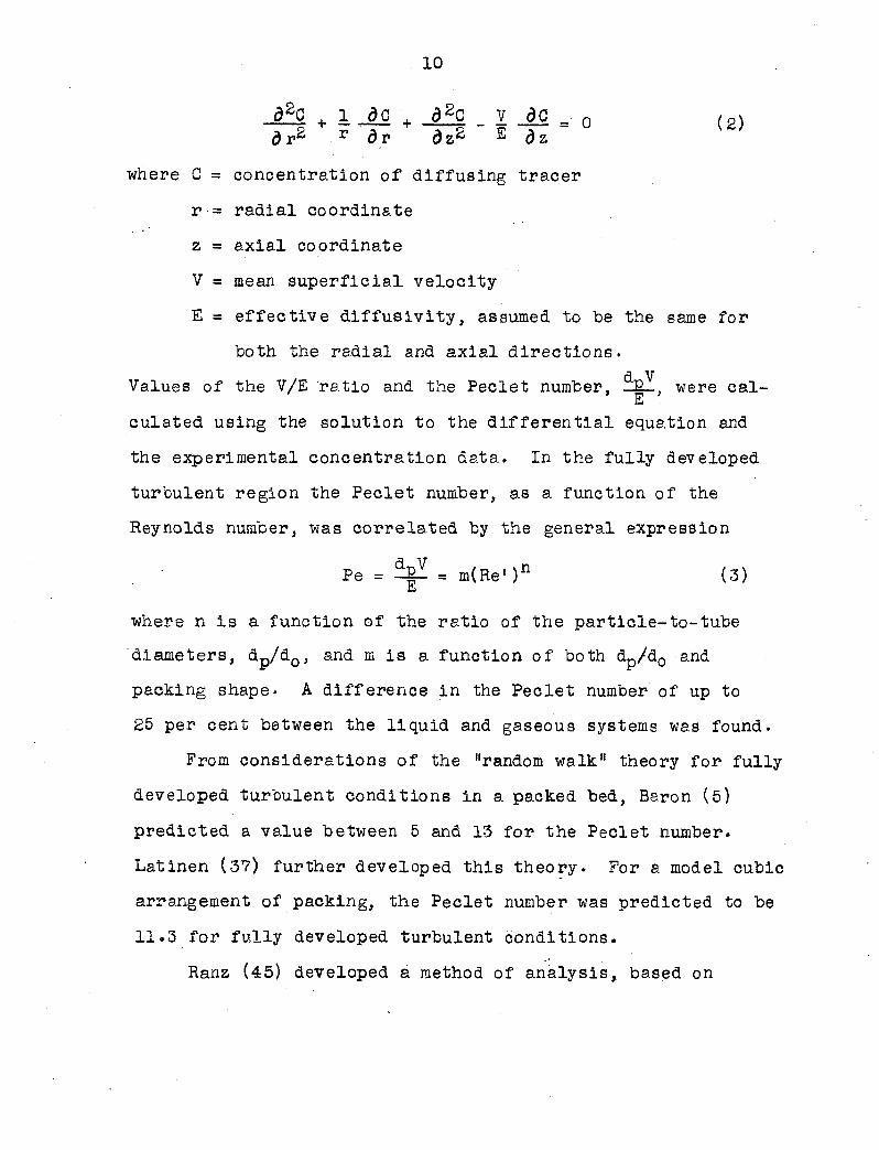
10

where G = concentration of diffusing tracer

r = radial coordinate

z = axial coordinate

V = mean superficial velocity

E = effective diffusivity, assumed to be the same for

both the radial and axial directions.

Values of the V/E ratio and the Peclet number, were cal-E

culated using the solution to the differential equation and

the experimental concentration data. In the fully developed

turbulent region the Peclet number, as a function of the

Reynolds number, was correlated by the general expression

Pe = —B— = m(Re')n (3) hi

where n is a function of the ratio of the particle-to-tube

diameters, dp/d0, and m is a function of both dp/d0 and

packing shape. A difference in the Peclet number of up to

25 per cent between the liquid and gaseous systems was found.

From considerations of the "random walk" theory for fully

developed turbulent conditions in a packed bed, Baron (5)

predicted a value between 5 and 13 for the Peclet number.

Latinen (37) further developed this theory. For a model cubic

arrangement of packing, the Peclet number was predicted to be

11.3 for fully developed turbulent conditions.

Ranz (45) developed a method of analysis, based on

11

properties of a single particle, for estimating and character­

izing transfer rates and pressure drops in packed beds. This

method appears to have application to the design and evalu­

ation of any transfer device which is an assemblage of a large

number of simply shaped interfaces arranged in an ordered or

random pattern. A value of 11.2 for the Peclet number was

predicted for fully developed turbulent conditions in a system

of spherical particles.

Fahien (24) solved the general diffusion equation for

steady-state mass transfer, allowing both the effective radial

diffusivity and the velocity to vary with radial position in

a fixed bed. The solution, considering boundary conditions

of a confining wall and a finite tracer injection tube, was

effected by replacing the differential equation with a set of

homogeneous linear difference equations. Axial diffusion was

assumed negligible when compared to bulk transfer. The effec­

tive radial Peclet number for carbon dioxide in air was found

to vary significantly with radial position, the variation

depending on the ratio of the particle diameter to the column

diameter• An explanation of the variation of Peclet number

with radial position was presented on the basis of an increase

in void fraction with radial position. Average values of the

Peclet number were found to increase with the particle-to-

column diameter ratio and to be substantially independent of

flow rate for Reynolds numbers greater than approximately 150.

12

Dorweiler (21) extended the data of Fahien (24) for

packed beds to very low flow rates. Some interaction of the

molecular and eddy mechanisms was illustrated by defining

molecular and eddy Peclet numbers and correlating them with

Reynolds number.

Plautz and Johnstone (43), applying the technique of

Bernard and Wilhelm (7), investigated both heat and mass

transfer in a packed bed. Air was used as the main stream

fluid, and sulfur dioxide as the tracer gas. Average Peclet

numbers were determined for isothermal conditions and for con­

ditions where a radial temperature gradient was impressed.

In the fully turbulent region, no effect was obtained; how­

ever, at low Reynolds numbers, the Peclet numbers for non-

isothermal conditions were less than those for isothermal

conditions, the decrease being more pronounced with smaller

packing.

Hanratty et al. (27) presented a theoretical analysis of

homogeneous isotropic systems involving turbulent mixing. The

analysis indicated that the eddy diffusivity becomes constant

only for relatively large times of diffusion. Although this

analysis was used in conjunction with experimental data from

a fluidized system, no characteristic parameter for a fluid­

ized bed was involved. Thus, a similar analysis may be applied

to any field of homogeneous isotropic turbulence.

Prausnitz and Wilhelm (44) measured time-average concen­

13

trations and concentration fluctuations directly above spheri­

cal packing in a fixed bed with a small, calibrated, movable

electrical conductivity cell. The time-average concentration

data were used to calculate values of a Peclet group which

appears as a parameter in a theory of concentration fluctua­

tions. The Peclet group had an average value of 10•5 for

Reynolds numbers larger than about 200, tube-to-particle

diameter ratios larger than about 10, and bed heights larger

than about 40 particle diameters.

Klinkenberg et al. (32) presented a mathematical study

of steady-state diffusion in a fluid moving in a cylindrical

tube at uniform velocity. Axial and radial diffusivities were

not assumed to be necessarily equal, but were assumed to be

constant throughout the bed. Boundary conditions imposed on

the steady-state diffusion equation corresponded to the

experimental arrangement of Bernard and Wilhelm (7) in their

determination of the eddy diffusion constants.

Hiby and Schummer (29) presented an analysis similar to

Klinkenberg et al. (32). An integration of the steady-state

diffusion equation, allowing for reflection at the tube wall

and for longitudinal diffusion, was given. The solution was

evaluated numerically for a range of conditions where longi­

tudinal diffusion was assumed negligible. In formulating

the diffusion equation the authors used tensor notation for

describing the anisotropic diffusion process.

14

Roemer et al. (49) calculated diffusion rates for a

2-inch i.d. column packed with 1/8- to 1/2-inch spherical par­

ticles and through which nitrogen flowed. Carbon dioxide was

injected into the center of the bed and its concentration

measured 4.75 inches downstream. Measurements were made for

Reynolds numbers between 3 and 80. They found that a point-

source solution of the diffusion equation gave values of

Peclet numbers about 10 per cent lower than a finite-source

solution. The effect of the magnitude of the axial Peclet

number on the radial Peclet number was indicated. The final

results were obtained by assuming that the axial and radial

Peclet numbers were equal.

Beek (6) discusses the utilization of diffusivity results

in the design of packed catalytic reactors. He suggests that

the radial diffusivity be assumed proportional•to the super­

ficial flow distribution. However, Richardson (46) has re­

cently shown that this assumption gives very poor agreement

between experimental and calculated mean conversions for the

oxidation of sulfur dioxide in a fixed-bed catalytic reactor.

He concludes that a variable radial diffusivity calculated

using experimental concentration data from a non-reactive

system gives significantly better agreement.

A mathematical model for predicting the mixing character­

istics of fixed beds of spheres was developed by Deans and

Lapidus (18, 19). The model is essentially a two-dimensional

15

network of perfectly stirred tanks. The predictions of the

model were compared with experimentally determined axial and

radial mixing parameters by means of the conventional partial

differential equation description of flow in fixed beds.

Introduction of a capacitance effect was shown to enable the

model to predict the abnormally low axial Peclet numbers

determined from the data of unsteady state liquid-phase

experiments. The application of the model to chemically

reactive systems was demonstrated.

Lamb and Wilhelm (34) analyzed the effects of packed bed

properties on local concentration and temperature patterns

using a "modified stochastic model". Their analysis appears

to be the first.attempt to develop a stochastic model for

fixed-bed equipment.

When a soluble material is injected suddenly into a

fluid flowing slowly through a tube, it spreads out along the

axial coordinate in both directions by the combined action of

molecular diffusion and the variation of velocity over the

cross-section. Taylor (57) showed analytically that with

certain assumptions the concentration distribution produced

is centered on a point which moves with the mean speed of

flow and is symmetrical about it in spite of the asymmetry of

the flow. Observed concentration distributions were used to

calculate a virtual coefficient of "diffusivity11 or axial

dispersivity. A derived relationship between this dispersiv-

16

ity and the molecular diffusion coefficient thus provided a

new method for determining diffusion coefficients. The coeffi­

cient so obtained was found to agree with that determined by

other means for potassium permanganate. A later paper de­

scribed (55) analytically the conditions under which disper­

sion of a solute in a stream of solvent could be used to

determine the molecular diffusion coefficient.

Later Taylor (56) extended his analysis to include turbu­

lent flow. Experimentally, brine was injected into a straight

3/8-inch pipe and the electrical conductivity was recorded at

a point downstream. The theoretical prediction was verified

by experiments with both smooth and .very rough pipes. An

estimate of the effect of the axial diffusion Indicated that

the correction was very small.

Although Taylor (55, 56, 57) treated experimental data

from pipe lines only, his mathematical analyses have no

restrictive parameters for such systems and thus may be easily

applied to fixed-bed systems.

A new basis for the analysis of dispersion of a solute

in a fluid flowing through a tube originally presented by

Taylor (55, 56, 57) was developed by Aris (l) . This analysis

removed the restrictions imposed on some of the parameters

at the expense of describing the distribution of solute in

terms of its moments in the direction of flow. The general

case of diffusion and flow in a straight tube is presented

17

together with its relation to some special cases.

Converse (16), by a theoretical development similar to

that used by Taylor '(56, 57) for pipe-line flow, showed the

relationship between the effective radial diffusivity, the

flow distribution, and the effective axial dispersivity for

flow in packed beds. Three calculations were made using a

constant effective radial Peclet number of 10. However, the

results did not indicate a monotonie trend and are perhaps

too limited from which to draw a sound conclusion.

In a reactor the time that the reacting species remain

within the system determines the overall conversion. In

reality fluid elements of the reactants spend various amounts

of time in the reacting zone and thus a distribution of resi­

dence times results. Danckwerts (17) showed the effects of

longitudinal dispersion on the distribution of residence times

for both open and packed tube systems. He further explained

how distribution functions for residence times can be defined

and measured for actual systems .

Kramers and Alberda (33) treated a sinusoidally varying

concentration input to a packed bed from both theoretical and

experimental viewpoints. Experimental results for axial dis­

persion in liquid flow through packed Raschig rings and for

back-mixing of a liquid flowing over the packing of an absorp­

tion column were compared with the predictions of two math­

ematical models: 1) the system was treated as a cascade of -

18

perfect mixers, and 2) the response of the system was regarded

as the combined result of perfect piston flow and a constant

coefficient of axial dispersion. The results were found to

deviate significantly from both models. The authors concluded

that perhaps such deviation was due, in part, to the non­

uniform velocity distribution in the bed. Nevertheless, sub­

sequent investigators have continued to treat the axial dis­

persion coefficient and the velocity as constants throughout

the bed with some degree of success in explaining their ex­

perimental results.

Deisler and Wilhelm (20) used a frequency response tech­

nique to determine mechanism constants for axial dispersion

in the fluid between particles in a bed of porous solids, pore

diffusion within the particles, and the composition equi­

librium between gases within and outside the.particles. Their

results indicated that the diffusion constant within the par­

ticles was on the order of a few per cent of the normal molec­

ular diffusion constant, but that the axial dispersion between

particles for Reynolds numbers between 4 and 50 is signifi­

cantly larger than for normal molecular diffusion.

A one-dimensional analysis of the boundary conditions

for a steady-state flow reactor with axial diffusion, uniform

flow distribution, and first order reaction was presented by

Wehner and Wilhelm (59). The simultaneous solution of the

three differential equations for the reaction, fore, and after

19

sections led to conclusions regarding reactor properties.

Contributions of axial mass transfer in the three parts of the

system to the course of the reaction in space were considered.

Levenspiel and Smith (39) presented methods for evaluat­

ing the axial dispersion coefficient from experimental measure­

ments. Examples were worked out and conditions for the appli­

cability of the model were discussed. The axial dispersion

coefficient was assumed to be independent of position for

either of the following two conditions: l) when the fluid

velocity and mixing are uniform, and 2) when the lateral dis­

persions of material (by either molecular diffusion or turbu­

lent mixing) is great enough to insure a uniform tracer con­

centration at any given cross section.

Several investigators added to the work of Lievenspiel

and Smith (39). Van der Laan (58) treated the problem in a

more general manner so as to include the case of finite pipe

length end that of a varying axial dispersivity. Aris (2)

showed that a suitable analysis was possible for tracer injec­

tions other than that of the delta function form. Bischoff

(8) presented a different procedure for finding first and

second moments from which the axial dispersivity could be cal­

culated.

MoHenry and Wilhelm (41) studied the axial mixing of

binary gas mixtures flowing in a random bed of spheres. The

systems Ng-Hg and CgH^-Ng were studied for Reynolds numbers

20

between approximately 100 and 400. For twenty-one determina­

tions the mean effective axial Peclet number was 1.88 + 0.15.

This is in excellent agreement with the theoretical value of

2.0 for the assumption that the bed of particles acts as a

series of perfect mixers, the number of mixers being equal to

the number of particles traversed between inlet and outlet

points in question. Thus the axial dispersivity for turbulent

flow of gases among particles appears to be about sixfold

larger than the effective radial diffusivity previously deter­

mined. This suggests that perhaps axial diffusion effects may

not be neglected in contacting devices such as adsorbers and

catalytic reactors.

Aris and Amundson (3) compared the solutions obtained

from the mixing cell model and a turbulent diffusive mechan­

ism model. They showed that the effective axial Peclet number

for agreement of the two must be about two, as a limiting case

for high Reynolds numbers. This result was further substan­

tiated by experimental data.

Ebach and White (23) used both a frequency response tech­

nique and a pulse function method to investigate the axial

mixing of liquids flowing through fixed beds of solids. Vari­

ables investigated were fluid velocity, particle diameter,

particle shape, and liquid viscosity. Effective axial Peclet

numbers varied from 0.3 to 0.8 for the range of Reynolds num­

bers from 0.01 to 150.

21

Carberry and Bretton (15), using a pulse input of dye in

water, essentially corroborated the results of Ebach and White

(23). They also briefly investigated the dispersion of a

pulse of air injected into a stream of helium flowing through

a gas chromatographic column. For Reynolds numbers less than

1 the axial dispersivity was found to be about equal to the

calculated molecular diffusivity of this gas system.

Experimental longitudinal "diffusivity11 data for packed

beds were obtained by Strang and G-eankoplis (54) using a fre­

quency response technique. Aqueous solutions of 2-naphthol

were used as tracers in a main water stream passing through

a 4.2-centimeter column packed with either 0.60-centimeter

glass beads, 0.63-centimeter Alcoa H-151 porous alumina

spheres, or 7x7-millimeter Raschig rings. Experiments were

conducted over a Reynolds number (based on mean interstitial

velocity in the bed) range of 14.1 to 46.9* Values of

» „ and Pez were determined as a function of Re .

Cairns and Prausnitz (13) investigated longitudinal mix­

ing properties of a water stream flowing through 2-inch and

4-inch tubes each packed with 1.3-, 3.0-, and 3.2-millimeter

spheres over the Reynolds number range 3 to 4500. Experiments

consisted of injecting a step function of salt solution

through a simulated plane source and measuring point concen­

tration breakthrough curves with electrical conductivity

probes. The results were reported in terms of an eddy "diffu-

22

sivity11 as a function of hydraulic radius and line velocity

which are proposed as the characteristic length and velocity

terms. The "diffusivities" are somewhat lower than those of

other investigators who used radially integrated rather than

point measurements of the breakthrough curve• It was shown

that the integrated results are too high because of a non-flat

velocity profile.

Cairns and Prausnitz (12) also studied the longitudinal

mixing properties in liquid-solid fluidized beds by means of

a step function response technique. The data reduction tech­

nique yielded non-flat "diffusivity" (actually dispersivity)

profiles. The results were consistent with the fact that the

fluidized bed may be considered as a transition between a

packed bed and an open tube.

Liles and Geankoplis (40) recognized and evaluated end

effects and the effect of column length on the axial disper­

sivity for liquids by frequency response studies. When end

effects were eliminated by an experimental technique for the

analysis of the inlet and outlet streams, no effects of length

on the dispersivity were found. However, when end effects

were artificially introduced by using void analytical sections

at the two ends, the dispersivity was found to decrease as

the length of the bed was increased until a certain point,

after which it remained constant with increase in length.

The overall results were in general agreement with the data

of others (13, 15, 23, 33, 54).

23

Robinson (47) calculated longitudinal dispersion coeffi­

cients for three "binary gas systems: helium-air, air-ethylene,

and nitrogen-ethylene. Calculations were made using data from

experimental measurements of the dispersion of a step function

input to columns packed with glass beads. The columns were

3/8-inch tubing packed with 0.0246-inch beads and were 10, 20,

and 40 feet in length, respectively• Coefficients were cal­

culated for the Reynolds number range from 0.03 to 1.0.

The effects of axial and radial diffusion on the mass

transfer coefficient for air flowing through a bed of

naphthalene pellets were evaluated by Bradshaw and Bennett

(ll). Values of the mass transfer coefficient as a function

of radial position were calculated from a differential mass

balance for naphthalene by graphical differentiation of the

various concentration profiles. Data on the radial variation

of the effective radial diffusivity (25), the superficial

velocity (51), and the void fraction (48) were used in the

final calculations. The axial term, involving a constant

axial Peclet number of 2.0, was included in the calculation,

but was found to have only minor effect on the final results.

The mass transfer coefficient was found to reach a maximum at

a dimensionless radial position of approximately 0.7 for

Reynolds numbers ranging from 438 to 9900.

Bischoff and Levenspiel (9) summarized the mathematical

models used to characterize dispersion of fluids in flowing

24.

systems. The models In which plug flow was assumed were dis­

cussed and compared. These models were shown to be special

cases of a very generalized model. In a second paper (10)

the authors related these plug flow models to the more general

models which do not assume plug flow nor constant values for

the dispersion coefficients.

Gottschlich (26) showed that the discrepancy between

axial dispersivities for gas-flow and liquid-flow experiments

may be explained by including the effect of a stagnant film. :

His analysis indicated that this mixing film has an effect on

dispersion only in un steady-state processes. The quantitative

nature of this film is such that it causes the effective axial

Peclet number for liquid-flow experiments to be smaller than

the theoretical value of 2.0 derived from the mixing cell

model. Thus, in steady state processes, such as a typical

catalytic reactor, the axial Peclet number should be approxi­

mately 2.0, whether for gas- or liquid-flow systems.

Houston (30) proposed a theory of elution chromatography

for the design of large-size chromatographic columns. The

dispersion of the solute band was attributed to axial disper­

sion. Associated experimental studies showed the effective

axial dispersivity to be dependent on the flow rate and size

of the solute sample. The effective axial Peclet number de­

creased from 0.11 to 0.06 (0.2 < Re' < 1.8) with increasing

flow (using benzene) and also decreased from 0.16 to 0.06 when

25

sample size was varied from 0.6 to 6.3 micromoles of solute

(using toluene).

Jacques and Vermeulen (31) studied the dispersion phe­

nomena in packed beds in both the axial and radial directions

to provide basic data for extraction tower design. Results

were presented as radial and axial Peclet numbers for both

one-phase and two-phase flow.

Sleicher (53) theoretically analyzed the effect of back-

mixing of either phase in an extraction column, which de­

creases the extraction efficiency, by means of an idealized

diffusion model. Calculations for a wide range of the model

parameters, a Peclet number for each phase, a mass transfer

number, and the usual extraction factor, were performed on a

digital computer. The principal results, presented in tabular

form, should be useful in the design and scale-up of extrac­

tion columns and in the interpretation of experimental results

from extractors and from some reactors in which a first-order

reaction occurs.

Hennico _et al. (28) determined axial dispersion coeffi­

cients for both the continuous and dispersed phases for the

two-phase countercurrent flow of water and kerosene in packed

columns. Their results indicated that longitudinal dispersion

is an important effect and should be calculated as an inde­

pendent factor in extraction column design.

Levenspiel and Bischoff (38) summarize the important

26

results from axial dispersion studies. They discuss the

utility of the axial dispersion model in the design of spe­

cific fixed-bed systems.

27

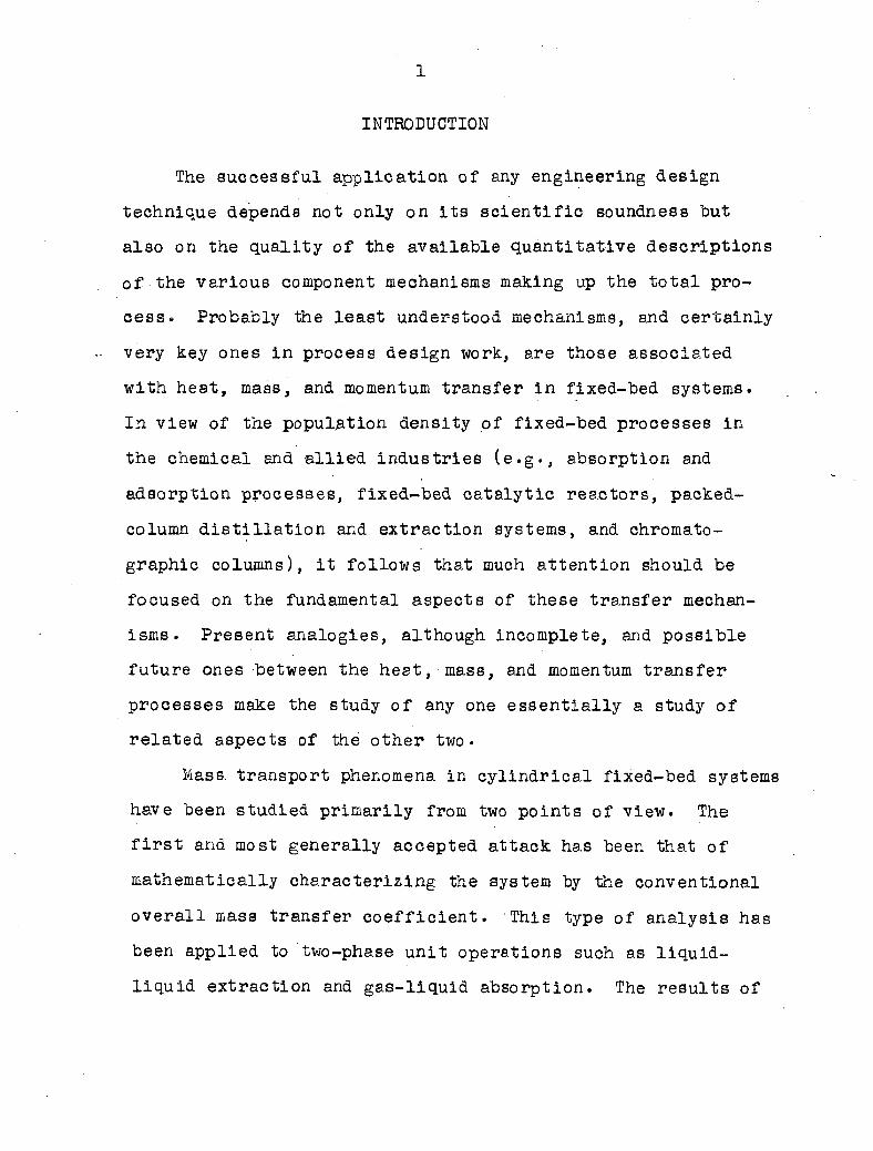
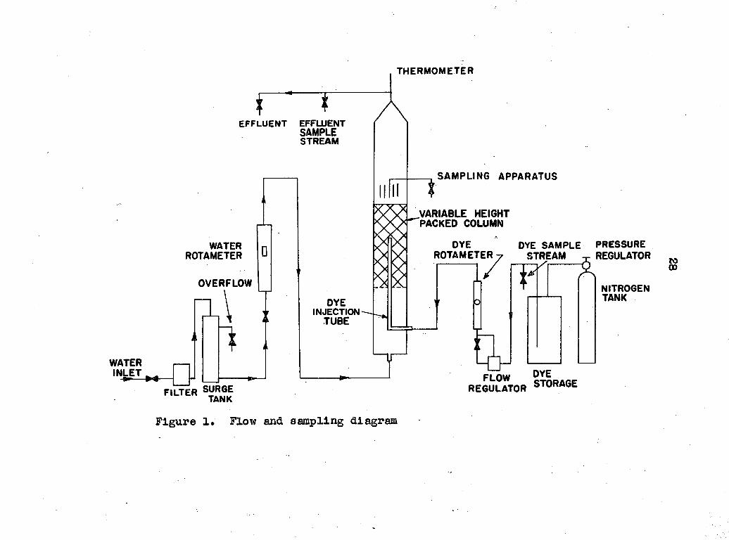
EQUIPMENT AND PROCEDURE

The experimental apparatus used in this study is shown

schematically in Figure 1. The equipment may be divided func­

tionally into a water filtering and metering section, a tracer

material metering section, a test column, a sampling section,

and an analytical instrument.

Water from the building supply was used as the bulk

stream liquid. Scale and dirt particles were removed from the

water stream by a 10-micron Cuno Micro-Klean filter. It was

further necessary to remove dissolved air from the water supply

since it caused bumping and generally unstable conditions in

,the test column. This was accomplished by passing the water

into the top of a 10-foot high, 4-inch diameter combination

surge, constant-head, and overflow tank. As the water flowed

down this column, the air had a tendency to escape upward to

the lower pressure area and consequently passed out the over­

flow line. After the water passed from the bottom of the

surge tank, it was metered by a 600-millimeter Brooks rota­

meter capable of measuring flow rates of 0.1 to 2.0 gallons

per minute. The flow rate was controlled by two globe valves:

a 3/4-inch valve preceding the filter and a l/2-inch valve

preceding the rotameter.

A 2.0 gram per liter water solution of fluorescein

disodium salt (dye) was used as the tracer material. The dye

was fed from a 4-liter storage tank pressurized by nitrogen.

THERMOMETER

EFFLUENT EFFLUENT SAMPLE STREAM

SAMPLING APPARATUS

VARIABLE HEIGHT PACKED COLUMN

PRESSURE REGULATOR

DYE ROTAMETER

DYE SAMPLE STREAM

WATER ROTAMETER

OVERFLOW NITROGEN TANK DYE

INJECTION TUBE

WATER INLET DYE

STORAGE FLOW REGULATOR SURGE

TANK FILTER

CD

Figure 1. Flow and sampling diagram

29

A two-stage pressure regulator was used to insure a constant

pressure on the storage tank. ,The dye flow rate was con­

trolled by a l/8-inch precision needle valve in conjunction

with a model 6-3BD-L Moore constant differential type flow con­

troller. The rate was measured by a 150-millimeter Brooks

rotameter with a flow rate range of 1.0 to 16.0 milliliters

per minute.

The test column consisted of a vertical 32-inch copper

pipe to which could be attached various lengths of transparent

acrylic tube. The average inside diameter was 3.97 inches.

A packing support, consisting of 0.045-inch stainless steel

wire screen with 0.2-inch square openings set on top of a

reinforced stainless steel circular frame, was held in posi­

tion 13 inches above the base plate of the column by three

3/16-inch bolts .

A 0.186-inch i.d. stainless steel tracer injection tube

entered the column at a point 3.5 inches above the base plate.

It was centrally located and held in place by the packing

support frame and its own rigid fastening through the wall

of the column. The injector extended to a point 8.0 inches

from the top of the copper pipe. When packing the column to

the level of the tip of the injection tube, a.spoke-wheeled

device was slipped over the tube to hold it rigidly in place.

The column was packed using a slow, rotary pouring motion.

The packing was 1/4-inch nonporous, ceramic, spherical

30

pellets (21). Because of the irregularity of the particles,.,

an effective diameter was determined by measuring the volume

of water displaced by 1300 pellets and calculating the diam­

eter equivalent to this number of perfect spheres. The

diameter thus determined was 0.262 inches.

The height of the packed bed above the injection tube was

varied by screwing additional lengths of the acrylic tube to

the base section. The connections were such that overlapping

grooves formed smooth inner seals.

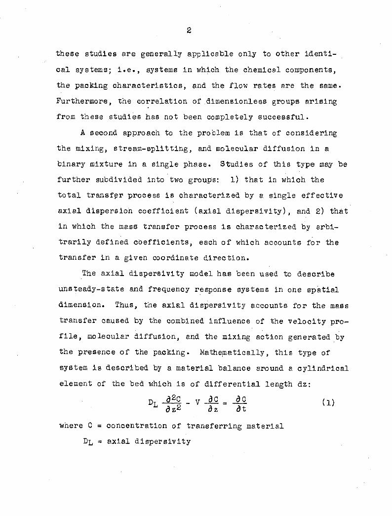
When the column had been packed to the desired height

above the injection tube, one of two sampling assemblies was

attached. Figure 2 depicts the multiple probe assembly in

position on top of the test column. This device was con­

structed such that at each radial position a number of equi­

angular probes entered a common outlet line downstream from

the top of the packing. The individual probes were l/8-inch

i.d. and 3/16-lnch o.d. The first radial position had four

individual probes 90 degrees apart. These were attached to

a common outlet which protruded through the column wall. On

the outside of the column a stopcock to control the sampling

rate was attached. Probes were located at six other radial

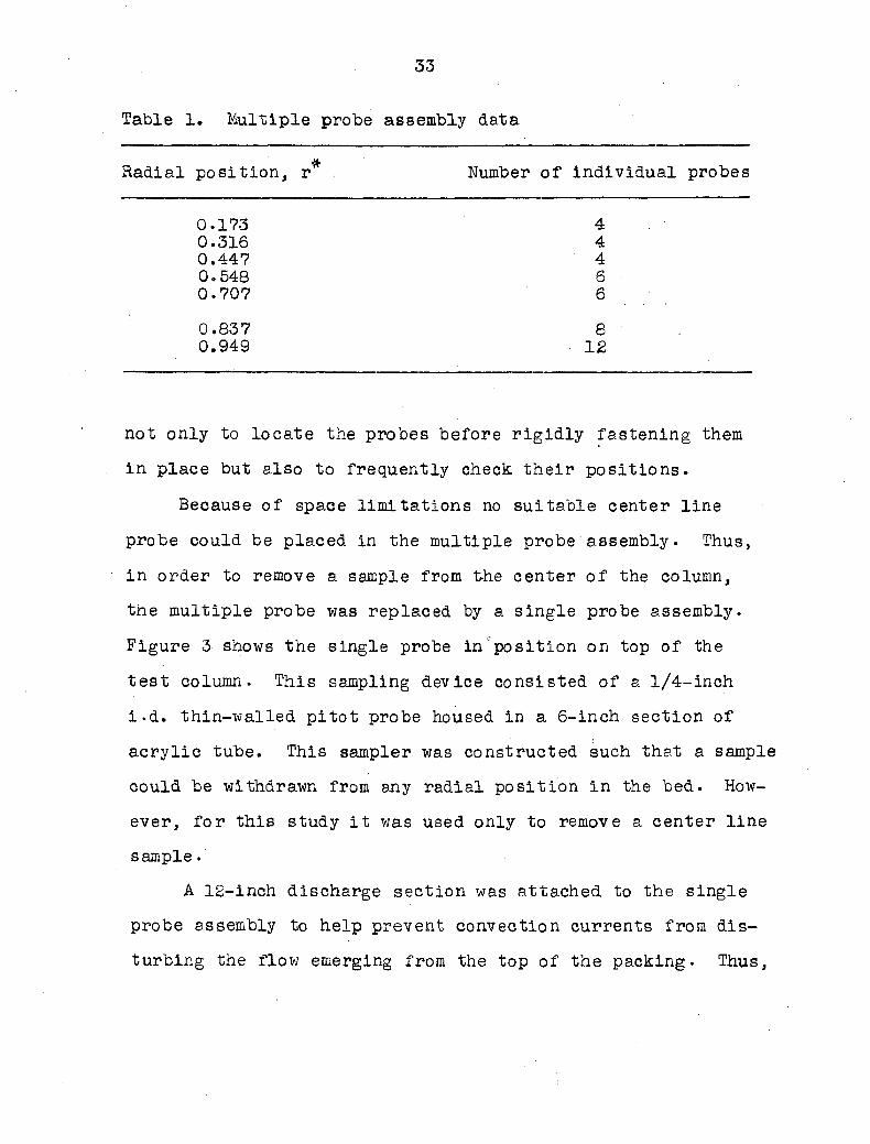
positions. Table 1 summarizes the probe positions.

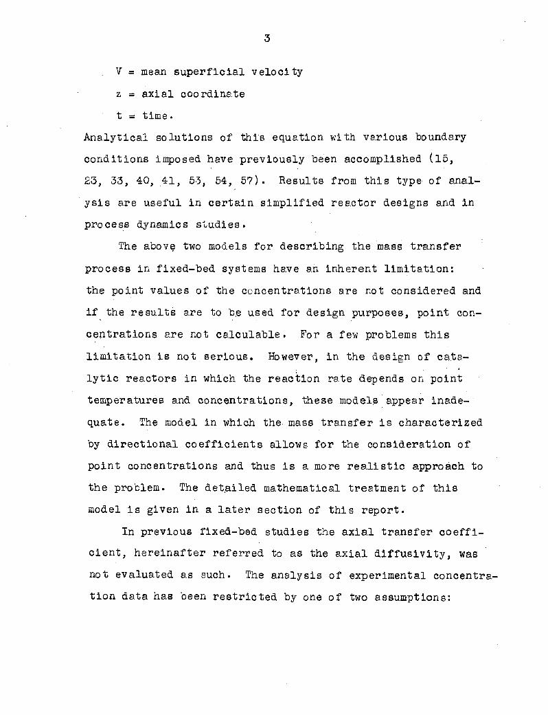
The individual probes were located in their respective

radial positions to within a tolerance of + 0.005 r* units

by using the plate shown in Figure 4. This plate was used

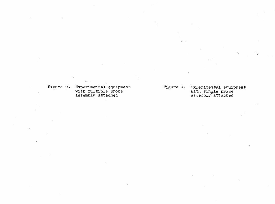
Figure 2. Experimental equipment Figure 3. Experimental equipment with multiple probe with single probe assembly attached assembly attached

32

33

Table 1. Multiple probe assembly data

Radial position, r* Number of individual probes

0.173 4 0.316 4 0.447 4 0.548 6 0.707 6

0.837 8 0.949 12

not only to locate the probes before rigidly fastening them

in place but also to frequently check their positions.

Because of space limitations no suitable center line

probe could be placed in the multiple probe assembly. Thus,

in order to remove a sample from the center of the column,

the multiple probe was replaced by a single probe assembly.

Figure 3 shows the single probe in position on top of the

test column. This sampling device consisted of a 1/4-inch

i.d. thin-walled pitot probe housed in a 6-inch section of

acrylic tube. This sampler was constructed such that a sample

could be withdrawn from any radial position in the bed. How­

ever, for this study it was used only to remove a center line

sample.

A 12-inch discharge section was attached to the single

probe assembly to help prevent convection currents from dis­

turbing the flow emerging from the top of the packing. Thus,

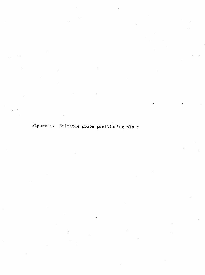
Figure 4. Multiple probe positioning plate

35

36

the column extended a total of 18 Inches above the packing,

For the multiple probe assembly the same result was achieved

by making the housing 18 inches in length.

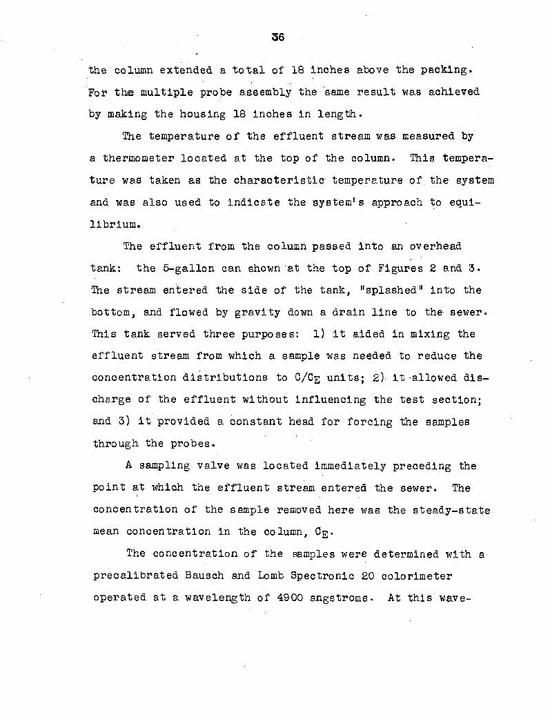
The temperature of the effluent stream was measured by

a thermometer located at the top of the column. This tempera­

ture was taken as the characteristic temperature of. the system

and was also used to indicate the system's approach to equi­

librium.

The effluent from the column passed into an overhead

tank: the 5-gallon can shown at the top of Figures 2 and 3.

The stream entered the side of the tank, "splashed" into the

bottom, and flowed by gravity down a drain line to the sewer.

This tank served three purposes: l) it aided in mixing the

effluent stream from which a sample was needed to reduce the

concentration distributions to C/Gg units; 2) It allowed dis­

charge of the effluent without Influencing the test section;

and 3) it provided a constant head for forcing the samples

through the probes.

A sampling valve was located immediately preceding the

point at which the effluent stream entered the sewer. The

concentration of the sample removed here was the steady-state

mean concentration in the column, Cg.

The concentration of the samples were determined with a

precalibrated Bausch and Lomb Spectronic 20 colorimeter

operated at a wavelength of 4900 angstroms. At this wave­

37

length the instrument had a range of 0.00 to 6.00 milligrams

dye per liter. Since some samples were of higher concentra­

tion, it was necessary to dilute them before measurement and

then to calculate the concentration of the original samples.

The experimental procedure was quite simple• The test

column was first packed to the desired height above the in­

jection tube. One of the two sampling assemblies was then

attached. The flow rates of the dye and water streams were

set to the desired values. The dye rate was fixed such that

the mean injection velocity was approximately equal to the

main stream superficial velocity. Depending on the flow rate

a period of 30 to 90 minutes was allowed for the system to

reach equilibrium. The criteria for equilibrium were that the

flow rates remained constant for approximately 30 minutes and

that thermal equilibrium was reached as indicated by the

temperature of the effluent stream. When using the multiple

probe sampler, samples were removed from all the radial posi­

tions simultaneously. The sampling rates were set such that

the mean linear velocity in each probe was approximately

equal to the mean superficial velocity in the column.

Accounting for the lag time appropriate to the flow rate a

"cup-mixed" sample was taken from the effluent stream. This

sample corresponded to the mean concentration in the column

at the time the radial samples were collected.

The above procedure was repeated for each desired flow

38

rate. Experiments were performed for three to five flow

rates after which the samples were analyzed with the colori­

meter .

When the desired experiments were completed with the

multiple probe, the single probe was used to establish the

center concentrations for the particular height of packing.

Then the packing height was changed and the entire process

was repeated.

39

MATHEMATICAL ANALYSIS

Development of the Boundary Value Problem

The total rate of a material transferred by the combined

processes of molecular and turbulent diffusion in a fluid

flowing in a duct has been mathematically expressed (52) by

J = - (DI + Et) • VC = - E • VC (4)

where J = mass transfer flux vector

C = concentration of transferring material

V = gradient operator

D = molecular diffusion coefficient

I = unit second-order tensor

I = 11 0 0\ 0 10

\0 0 1

= turbulent diffusivity tensor

/Etrr Etrgf EtrzN

Et = Etszfr Etg# Etjz(z m cylindrical / coordinates

\Etzr Etz^ Etzz/ (r> z)

E = total diffusivity tensor

/Err Er^ ErzN

E = I E^r E^ E^z

\Ezr Ezgf Ezz'

Equation 4 expresses the molecular and turbulent pro­

cesses as though they occur in parallel. For flow in an

40

unpacked tube this may be partially correct, although the

turbulent transport process is itself nevertheless influenced

by molecular diffusion. However, in any case, it must be

recognized that Equation 4 is an arbitrary definition of E,

which is only an empirical coefficient.

If one accepts the general differential equation descrip­

tion of fixed-bed processes (i.e., one assumes a"smooth vari­

ation of properties on a macroscopic scale), a description of

the mass transfer process taking place in the fluid moving in

the interstices of the packing may be written

J = - E • VC (5)

where the separation of the molecular and turbulent processes

is not indicated. It is felt that no distinct separation of

the two processes can be made for a fixed-bed system. The

diffusivity for the packed bed defined by Equation 5 must

not be confused with that of the unpacked tube defined by

Equation 4. Each must be determined by the analysis of ex­

perimental data from its respective physical configuration.

Unless otherwise stated, the term "diffusivity11 as used in

this work will be that associated with a packed bed. Un­

doubtedly the components of the diffusivity tensor are very

complicated functions of the column diameter, packing charac­

teristics, flow rate, and perhaps fluid properties (especially

at low flow rates) .

Using the above nomenclature the general equation for

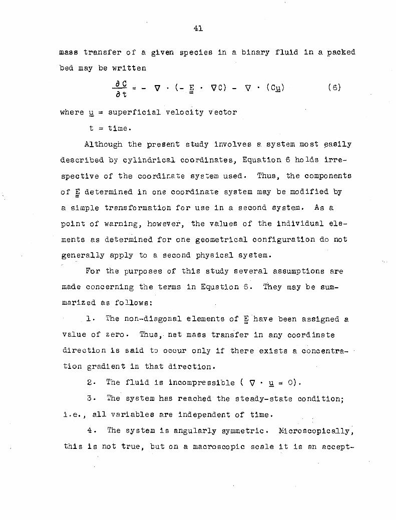
41

mass transfer of a given species in a binary fluid in a packed

bed may be written

— = - V • (- E • VC) - V • (Ou) (6) d t

where u = superficial velocity vector

t = time.

Although the present study involves a system most easily

described by cylindrical coordinates, Equation 6 holds irre­

spective of the coordinate system used. Thus, the components

of E determined in one coordinate system may be modified by

a simple transformation for use in a second system. As a

point of warning, however, the values of the individual ele­

ments as determined for one geometrical configuration do not

generally apply to a second physical system.

For the purposes of this study several assumptions are

made concerning the terms in Equation 6. They may be sum­

marized as follows :

. 1. The non-diagonal elements of E have been assigned a

value of zero. Thus, net mass transfer in any coordinate

direction is said to occur only if there exists a concentra­

tion gradient in that direction.

2• The fluid is incompressible ( V • u = 0).

3. The system has reached the steady-state condition;

i.e., all variables are independent of time.

4. The system is angularly symmetric. Microscopically,

this is not true, but on a macroscopic scale it is an accept­

42

able assumption.

5. The system is macroscopically homogeneous in the

direction of net flow.

6. The radial diffusivity, Err, hereinafter denoted by

Er and the axial diffusivity, Ezz, hereinafter denoted by Ez,

are functions of radial position only.

7. Net flow is- in the axial direction only and the

flow distribution is a function of radial position only.

Under these assumptions Equation 6, expressed in cylindrical

coordinates, becomes

r ~§7 (rEr(r)y;) + Ez(r) = uz(r) ' (7)

For calculational purposes it is convenient to write

Equation 7 in dimensionless form. The following dimensionless

variables are used:

r* = r/r o # /

fp = rp/?o

z* = z/r0

&p = &p/ro

v* = uz(r)/V

v*(?p) = uz(rp)/V

C* = C/CE

P = Er(r)/Er(rp)

Per^rp) - dp ' uz(rp)/Ep(rp)

Pez = dp • uz(r)/Ez(r)

( 8 )

43

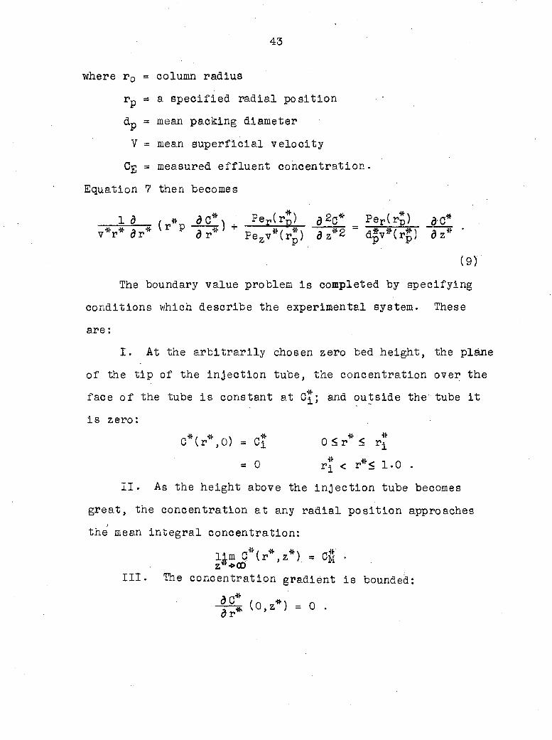
where r0 = column radius

rp = a specified radial position

dp = mean packing diameter

V = mean superficial velocity

Cg = measured effluent concentration.

Equation 7 then becomes

1 à i » _d_C* \ _Per^rx>^ d Per(rp) &C* >V dr* U P dr* ' Pezv*(r*) d z*2 = a*v*(r«) dz* '

(9)

The boundary value problem is completed by specifying

conditions which describe the experimental system. These

are :

I. At the arbitrarily chosen zero bed height, the plane

of the tip of the injection tube, the concentration over the

face of the tube is constant at 0^; and outside the tube it

is zero:

C*(r*,0) = C* 0<r* < r*

= 0 r* < r*< 1.0 .

II. As the height above the injection tube becomes

great, the concentration at any radial position approaches

the mean integral concentration:

III. The concentration gradient is bounded:

to.»*) = o -

44

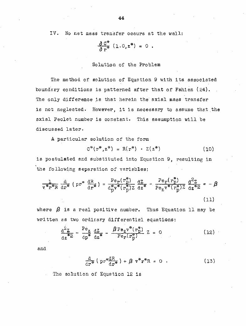
IV. No net mass transfer occurs at the wall:

(1.0, z*) = 0 .

Solution of the Problem

The method of solution of Equation 9 with its associated

boundary conditions is patterned after that of Fahien (24).

The only difference is that herein the axial mass transfer

is not neglected. However, it is necessary to assume that the

axial Peclet number is constant. This assumption will be

discussed later.

A particular solution of the form

C*(r*,z*) = R(r*) • Z(z*) (10)

is postulated and substituted into Equation 9, resulting in

the following separation of variables:

1 d_ , * dR_ x Per(rg) dZ Per(rg) d2Z _ _ R

vVR dr* (P dr*' d*v*(r*)Z dl^ Pe%v*(r*)Z a%*2 ~ P

(11)

where jS is a real positive number. Thus Equation 11 may be

written as two ordinary differential equations :

(12) d £Z _ £f i dZ_ _ f fpezv*(r£) z = 0

az*2 dp* dze " Per(i-J)

and

& ( ) + J8 v*r*R = 0 . (13) dr 1 r dr1

The solution of Equation 12 is

45

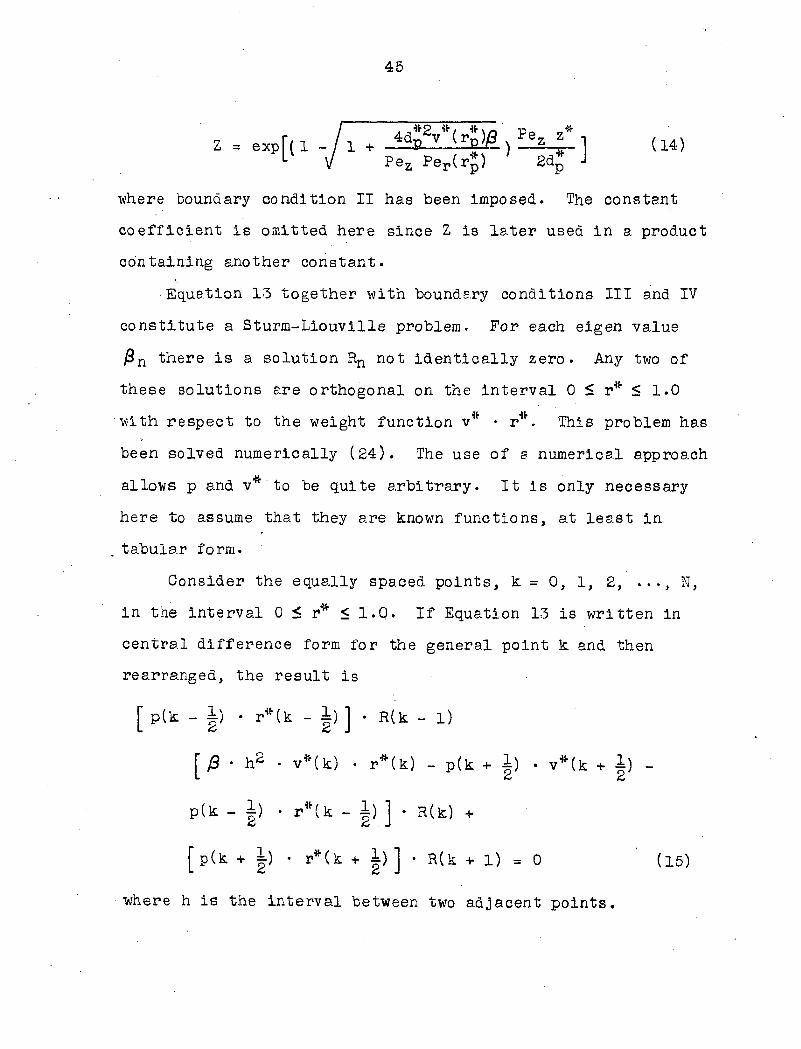
• = • • » [ < • - / ' * f SSI1''-!#] ""

where boundary condition II has been imposed. The constant

coefficient is omitted here since Z is later used in a product

containing another constant.

Equation 13 together with boundary conditions III and IV

constitute a Sturm-Liouville problem. For each eigen value

j3n there is a solution Rn not identically zero. Any two of

these solutions are orthogonal on the interval 0 < r* < 1.0

with respect to the weight function v* • r*. This problem has

been solved numerically (24). The use of a numerical approach

allows p and v* to be quite arbitrary. It is only necessary

here to assume that they are known functions, at least in

tabular form.

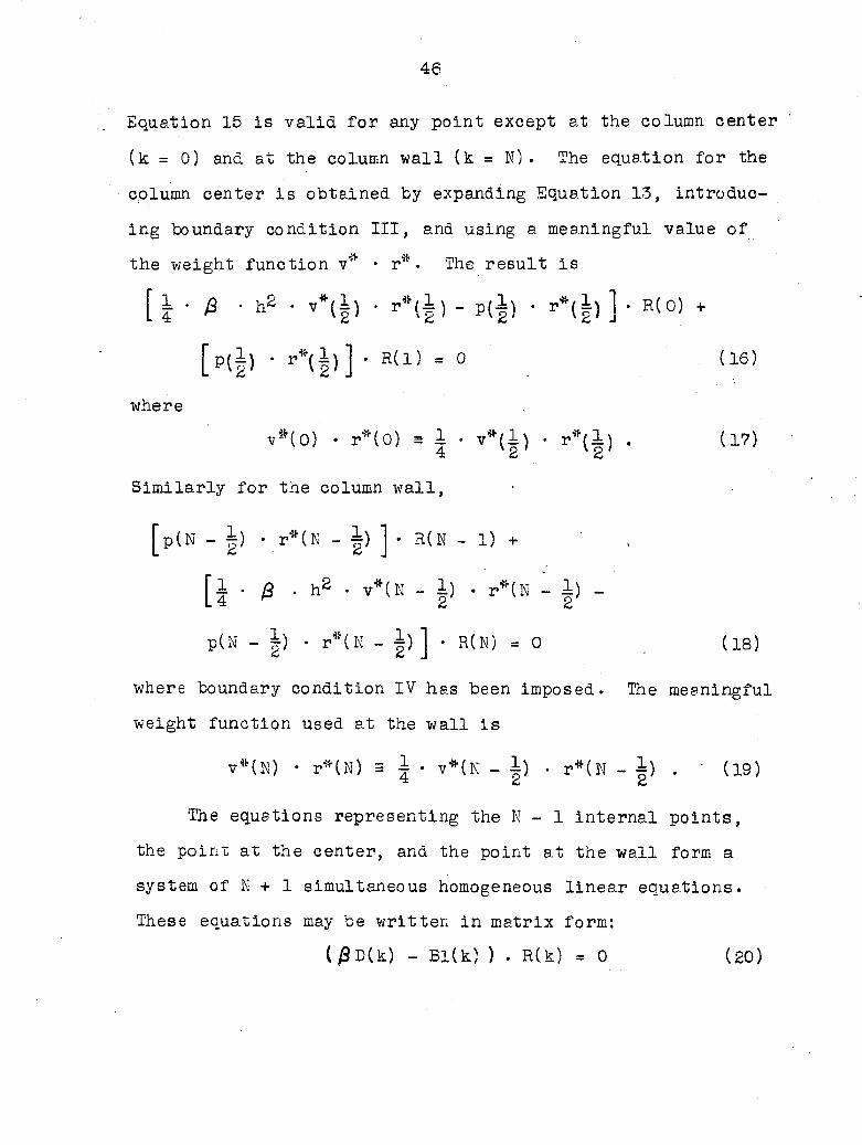
Consider the equally spaced points, k = 0, 1, 2, .N,

in the interval 0 < r* < 1.0. If Equation 13 is written in

central difference form for the general point k and then

rearranged, the result is

[ p(k - i) • r"(k - i)] • R(k - l)

[ /3 • h2 • v*(k) • r*(k) - p(k + | ) • v*(k + 1) -

p(k - i) • r*(k - i) ] • R(k) +

[ p(k + |) • r*(k + i) ] • R(k + 1) = 0 (15)

where h is the interval between two adjacent points.

46

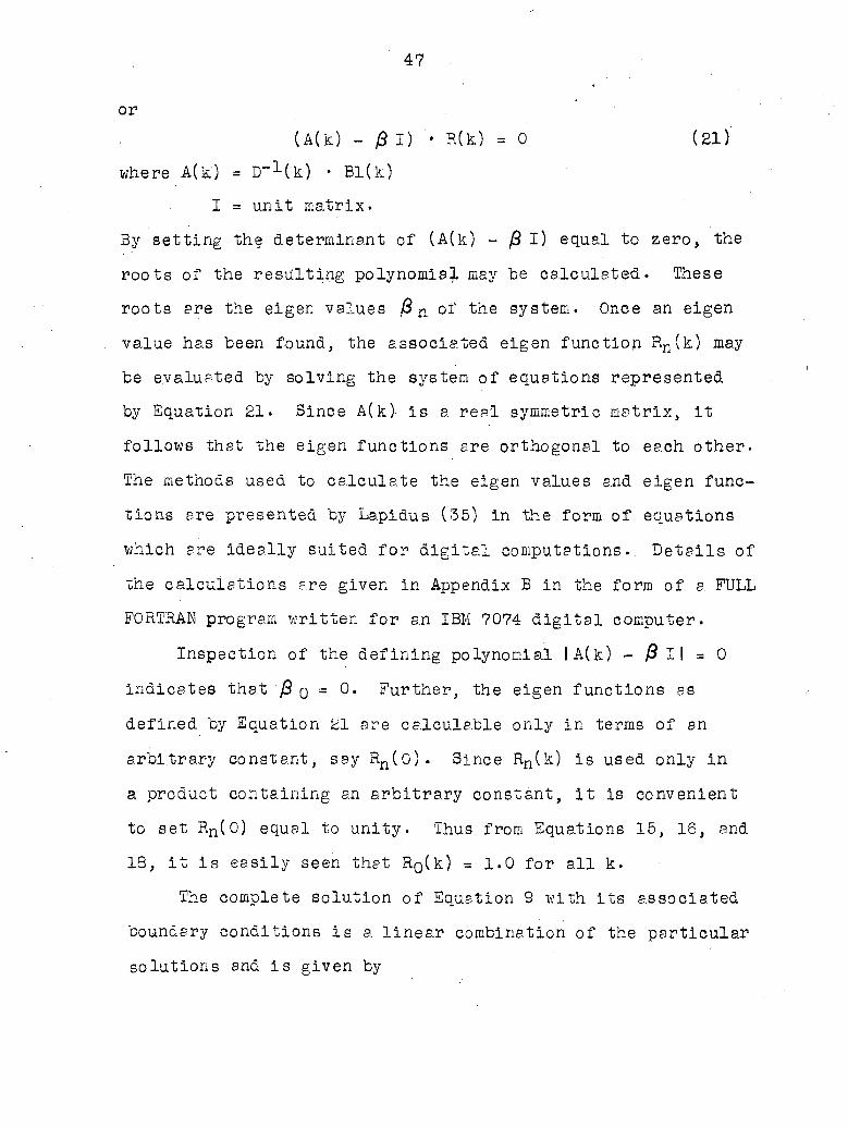
Equation 15 is valid for any point except at the column center

(k = 0) and at the column wall (k = N). The equation for the

column center is obtained by expanding Equation 1-3, introduc­

ing boundary condition III, and using a meaningful value of

the weight function v

[ J • /3 - - v"(|

[ p ( |> ' ' * ( | ) ]

where

The result is

r*(i) - V { h

R( 1 ) = 0

R(0) +

v**(0) • r*(0) 2 1 • v*(l) 4 2

Similarly for the column wall,

[p(N - |) • r*(N - |) ] • R(N - 1) +

(16 )

(17)

v*(N - 1) • r*(N - 1) -2 2 [ I - »

p(N - ̂ ) • r*(N - 7j) j • R(N) = 0 (18)

where boundary condition IV has been imposed. The meaningful

weight function used at the wall is

v*(N) r*(N) s J • v*(N - 1) - r*(N - | ) (19)

The equations representing the K - 1 internal points,

the point at the center, and the point at the wall form a

system of M + 1 simultaneous homogeneous linear equations.

These equations may be written in matrix form:

(#D(k) - Bl(k) ) . R(k) = 0 (20)

47

or

(A(k) - £ I) • R(k) = 0 (21)

where A(k) = D-1(k) • Bl(k)

I = unit matrix.

By setting the determinant of (A(k) - /Si) equal to zero, the

roots of the resulting polynomial may be calculated. These

roots are the eigen values B n of the system. Once an eigen

value has been found, the associated eigen function Rn(k) may

be evaluated by solving the system of equations represented

by Equation 21. Since A(k) is a real symmetric matrix, it

follows that the eigen functions are orthogonal to each other.

The methods used to calculate the eigen values and eigen func­

tions are presented by Lapidu s (35) in the form of equations

which are ideally suited for digital computations. Details of

the calculations are given in Appendix B in the form of a FULL

FORTRAN program written for an IBM 7074 digital computer.

Inspection of the defining polynomial IA(k) - P II = 0

indicates that ft q = 0* Further, the eigen functions as

defined by Equation 21 are calculable only in terms of an

arbitrary constant, say Rn(0) . Since Rn(k) is used only in

a product containing an arbitrary constant, it is convenient

to set Rn(0) equal to unity. Thus from Equations 15, 16, and

18, it is easily seen that RQ( k) = 1.0 for all k.

The complete solution of Equation 9 with its associated

boundary conditions is a linear combination of the particular

solutions and is given by

48

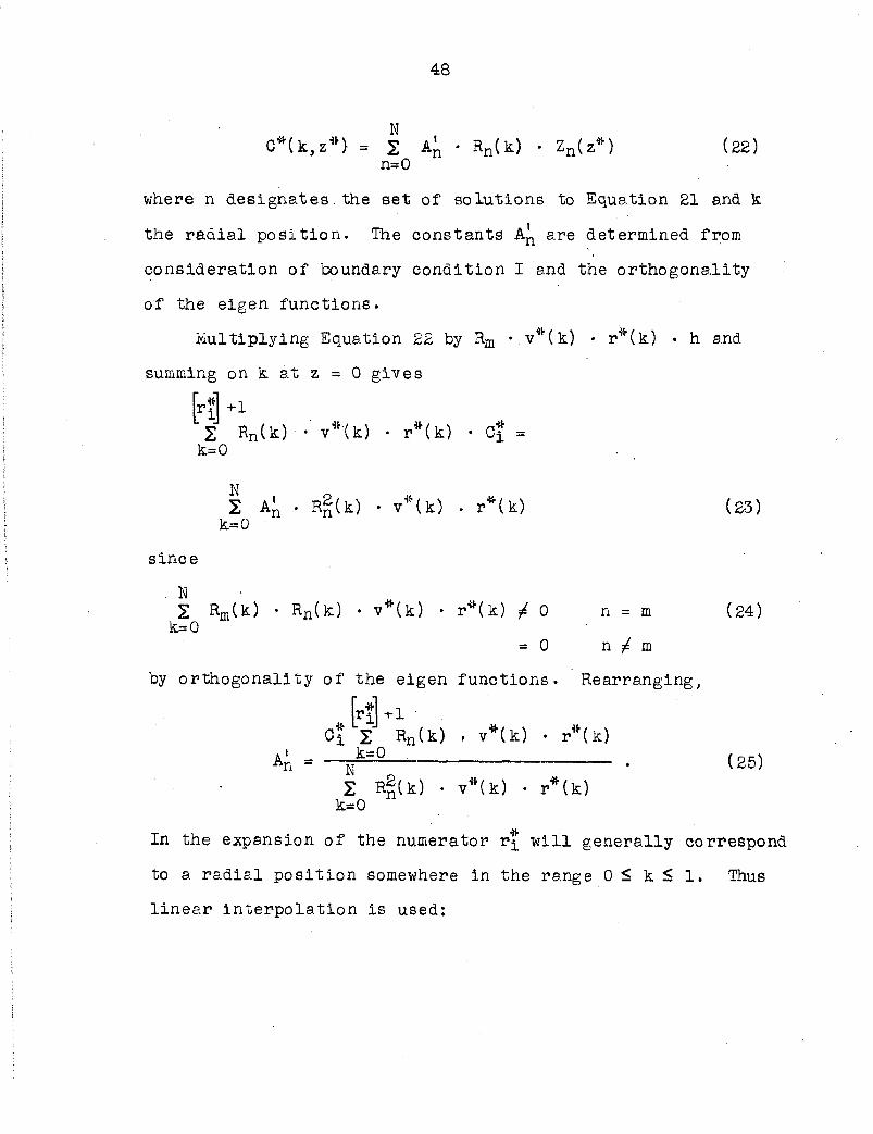
N C*(k,z*> = 2 • Rn(k) • Zn(z*) (22)

n=0

where n designates the set of solutions to Equation 21 and k

the radial position. The constants are determined from

consideration of boundary condition I and the orthogonality

of the eigen functions.

Multiplying Equation 22 by Rm • v*( k) • r*(k) • h and

summing on k at z = 0 gives

[rï]+l

2 Rn(k) ' v*'(k) - r*(k) • C* = k=0

N 2 A^ . R§(k) • v*(k) . r*(k) (23) k=0

since

. N 2 Rm(k) • Rn(k) • v ( k ) • r * ( k ) / 0 n = m (24) k= 0

= 0 n / m

by orthogonality of the eigen functions. Rearranging,

U] +i Ci 2 R n ( k ) ' v*(k) • r*(k)

4, ' /"° - (26)

2 R§(k) • v*(k) • r*(k) k=0

In the expansion of the numerator r* will generally correspond

to a radial position somewhere in the range 0 < k < 1. Thus

linear interpolation is used:

49

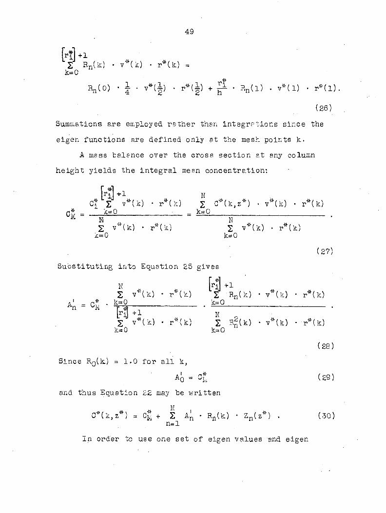
lrî l+1 2 Rn(k) • v*(k) • r*(k) = ln k=0

Rn(0) • l • v*(|) • r*(|) + ̂ • Rn( 1 ) • v*(l) • r*(l)

(26)

Summations are employed rsther than integrations since the

eigen functions are defined only at the mesh points k.

A mass balance over the cross section at any column

height yields the integral mean concentration:

[ri] +1 , N CÎ 2 v*(k) • r*(k) 2 G*(k,z^) • v^(k) • r*(k)

0Ï = 1=0 - k=0 'M N , N 2 v^(k) - r*(k) % v*(k) - r*(k) k=0 k=0

(2?)

Substituting into Equation 25 gives

N , [riJ +1

2 v*(k) • r^(k) 2 Rn ( -0 * v*(k) • r*(k) A „ = CI,: y - Ok ' # ï=2

riJ +1 N 2 v*(W - r*(k) 2 R%(k) - v*(k) - r*(k)

k=0 k=0 n

(28)

Since R0(k) = 1.0 for all k,

AQ = 0^ ( 29 )

and thus Equation 22 may be written

1\T

C*(k,z*) = + 2 A% - R%(k) - Z%(z*) . (30) n=l

In order to use one set of eigen values end eigen

50

functions for computer calculations involving more than one

set of concentration data, new constants may be defined such

that

Bn = An/C% . (31)

Equation 30 then becomes

N C*(k,z*) = Cm(i + 2 Bn • Rn(k) • Zn(z*))« (32)

n=l

The procedure for calculating the constants Bn is an integral

part of the computer program given in Appendix B.

Treatment of Experimental Data

The above solution implies that if one knows p, v * , Pez,

and Pep(rp), the concentration may be calculated for the gen­

eral point (k,z*). However, the problem at hand is somewhat

different. It may be stated as follows: Given an experi­

mentally determined flow distribution v* and sufficient con­

centration data find values of the radial Peclet number

Per(rp) and the axial Peclet number Pez, and determine the

radial variation of the radial diffusivity Er (i.e., find ,

how p varies with r*)• Consider first the function p.

Determination of the radial variation of p

Since fin becomes increasingly larger with n, it follows

that Zn becomes progressively smaller. In turn the successive

terms in Equation 30 decrease in size very rapidly. Thus for

51

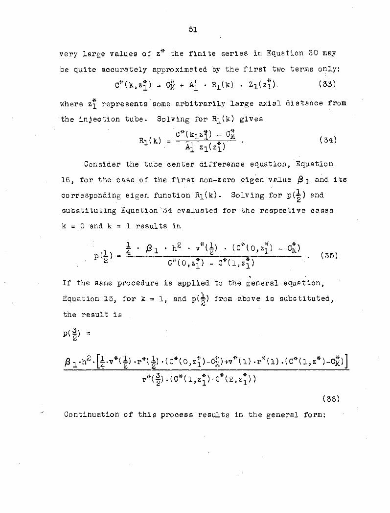
very large values of z* the finite series in Equation 30 may

be quite accurately approximated by the first two terms only:

C*(k,z*) = Cm + • Zi(z*) (33)

where z* represents some arbitrarily large axial distance from

the injection tube. Solving for R]_(k) gives

Rl(k) = C J'îuî)0* ' (34)

Consider the tube center difference equation, Equation

16, for the- case of the first non-zero eigen value j and its

corresponding eigen function R]_(k). Solving for p(^) end

substituting Equation"34 evaluated for the respective cases

k = 0 and k = 1 results in

E,l) J • -h« • (0»tO,.î) -OS) ,

If the same procedure is applied to the general equation,

Equation 15, for k = 1, and p(^) from above is substituted,

the result is

P(f> -

i*h2«[ j*v* ( i ) »r* ( i ) •(C'"'(0,z£)-Cy1)+v*( l) »r*(l) - ( C* ( 1, z*)—Cm)]

r*(§).(C*(l,z*)_C*(2,z*))

(36)

Continuation of this process results in the general form:

52

p(k + g) =

/ô 1 • h2 • 2 v#(k) • r*(k) • (C^(k,z*) - ) k=0

T*(k + 1) . (C*(k,Z^) - 0*(k + 2 '

(37)

Recalling the defining expression for the function p,

p = Er(r)/Ey(rp) , (38)

it is now convenient to fix r^, and thus rp, such that

Tp = r*(k + = r*(i) = h/2 . (39)

I k=0

Then

p(r*) = p(|) = 1.0 (40)

and Equation 35 may "be rearranged to give

. (41) I • V*(|) . (0*(0,ïï) - o|)

Substituting into Equation 37 gives

p(k + |) =

(C*(0,z*)_C*(l,z*)- Z v*(k).r*(k).(C*(k,zï)_CM) k=0

4*v*(g) • r*(k+^) • (C'M,(0,z*)-Cm) "(C*(k,z*)-C*(k+l,z*) )

(42)

Equation 42 may be used to determine the function p, and

thus the radial variation of the radial diffusivity, from

experimental concentration and flow distribution data. Fur­

thermore, the corresponding eigen values and eigen functions

53

may then be evaluated from the system of equations represented

by Equation 21. These results in turn may be used to calcu­

late Peclet numbers.

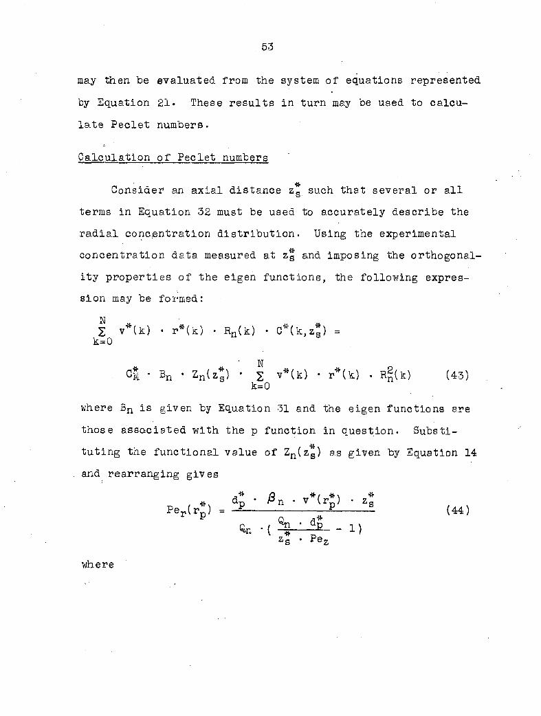
Calculation of Peclet numbers

Consider an axial distance z* such that several or all

terms in Equation 32 must be used to accurately describe the

radial concentration distribution. Using the experimental

concentration data measured at Zg and imposing the orthogonal­

ity properties of the eigen functions, the following expres­

sion may be formed :

N 2 v*(k) • r*(k) - Rn( k) • C*(k,z*) = k=0

N C| • Bn • Zn(Zg) • 2 v*(k) ' r*(k) • R^(k) (43)

k=0

where Bn is given by Equation 31 and the eigen functions are

those associated with the p function in question. Substi­

tuting the functional value of Zn(Zg) as given by Equation 14

. and rearranging gives

p.r(pJ, . < • • T'('P • 4 (44,

zs • Pez

where

54

K S v*U) • r*(fc) • R„(k) • C*(k,z%)

On = ln [SsO - 1. (45)

Cm • Bn • 2 v#U) • r*(k) • s2(k) k=0

Equation 44 holds for any n > 0. Thus there are N inde­

pendent linear equations in Per(rp) and Fez. Solving the .

resulting equations where n is successively one and two gives

Pez = dP ' '^1 " ^ - 02 ' ̂ . (46) zs ' ( ̂ 1 ' ®>2 ~ @2 ' ̂

The numerical value for Pez calculated here is then used in

Equation 44 in order to calculate Per(rp)•

Prediction of Concentration Distributions

When the preceding methods are used to calculate p,

Pez, and Per(r^) from experimental data, one is not assured

that the reverse procedure will reproduce exactly the original

concentration distributions. It is interesting to compare

the distributions as predicted by Equation 32 using calculated

values of p, Pez, Per(rp), and the associated eigen values

and functions with the original experimental concentration

data. The degree of agreement of the. two represents to some

extent a measure of the validity of the boundary value problem

as a model for describing the mass transfer process.

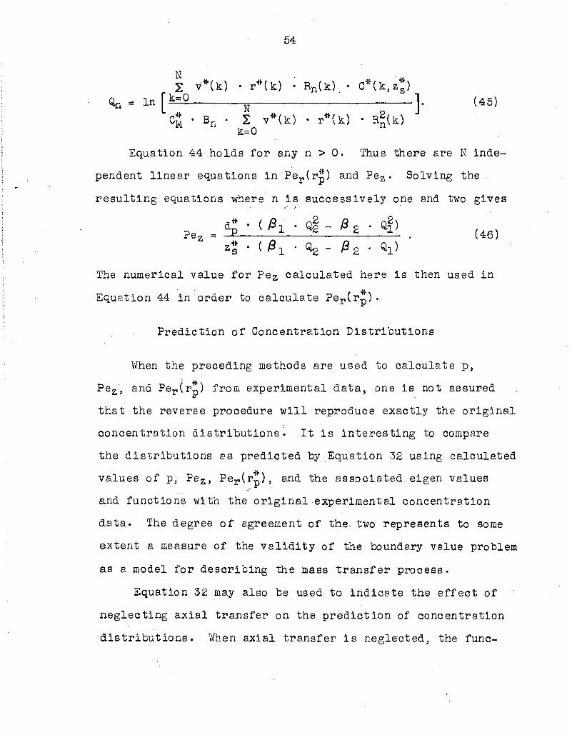
Equation 32 may also be used to indicate the effect of

neglecting axial transfer on the prediction of concentration

distributions. When axial transfer is neglected, the func­

55

tional value of Zn(z*) becomes

J Per(r*)

(47)

and Equation 44 reduces to

( 4 8 )

Thus the effective radial Peclet number may be calculated

directly for the case n = 1. This value of Per(rp) may then

be used in Equation 32 where the functional value of Zn(z*)

is given by Equation 47 to predict the concentration dis­

tribution for the case when axial transfer is neglected.

56

RESULTS AND DISCUSSION

The scope of this investigation was chosen such that the

effect of neglecting axial transfer on the prediction of con­

centration distributions would most likely be significant.

The flow rate range includes points in the upper transition

region just below the accepted fully developed turbulent

region and those which are perhaps in the lower flow region

of practical engineering applications.

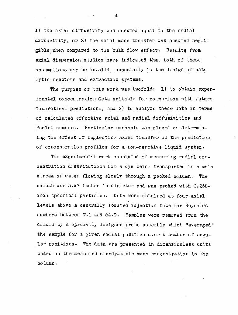
Experimental Concentration Data

The experimental data consist of radial concentration

distributions for various axial distances downstream from a

centrally located tracer injector. Typical distributions are

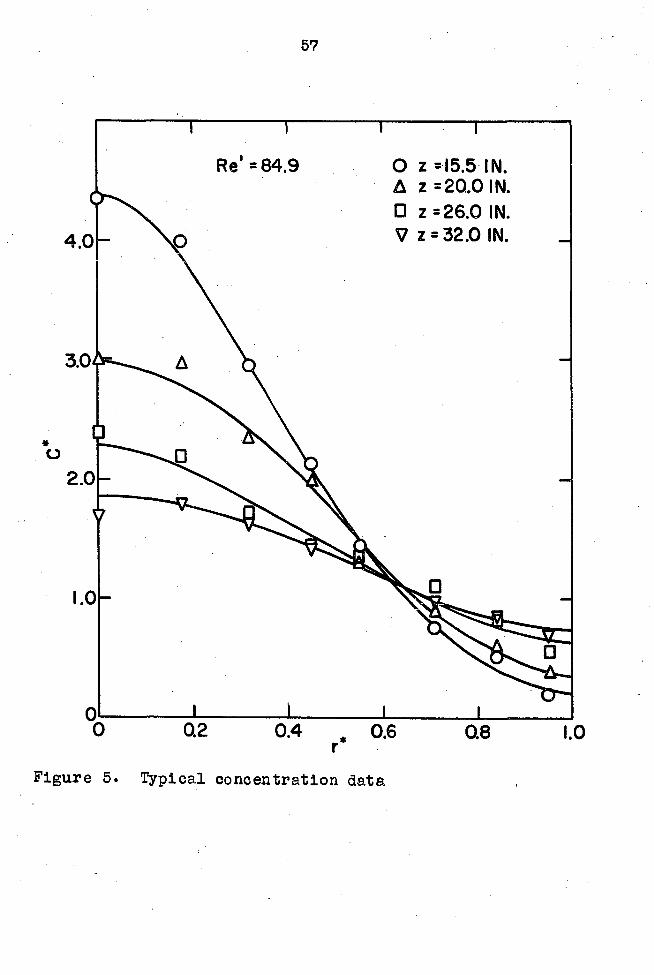
shown in Figure 5. The experimental data are tabulated in

Table 6.

During experimentation the ambient temperature and the

water temperature changed from day to day. These changes

were indicated by the effluent stream temperature variations.

The temperature data reported in Table 6 represent the range

of the temperature of the effluent stream for all experiments

performed for each particular flow rate. These data were

considered only in the determination of the kinematic vis­

cosity used to calculate the Reynolds numbers. Although the

temperature is known to have some effect on the rate of mass

transfer, this effect was not considered herein since the

57

Re'=84.9 O z =15.5 IN. A z =20.0 IN. • z =26.0 IN. V z = 32.0 IN. 4.0

3.0

*

O

2.0

1.0

0.2 0.4 0.6 Q8

Figure 5. Typical concentration data

58

overall temperature range was only 6.5°C.

The accuracy of the individual concentration determina­

tions depended essentially on the reproducibility of the

calibration of the colorimeter. The calibration was obtained

by determining the transmittances for standard concentrations

covering the range of interest. Periodic checks indicated

that the transmit tance could be reproduced with a maximum

deviation of approximately 3 per cent of its mean value for

all concentration levels.

Final consideration of the experimental data concerns

its representation of the overall mass transfer process.

Bernard and Wilhelm (7) repacked and hammered the test section

until the single diameter traversed resulted in a fairly

symmetrical concentration profile. Average values of the

radial diffusivity and Peclet number were then calculated by

applying a least squares technique to the data. Such a pro­

cedure, however, may not yield representative parameters of

the overall mass transfer process.

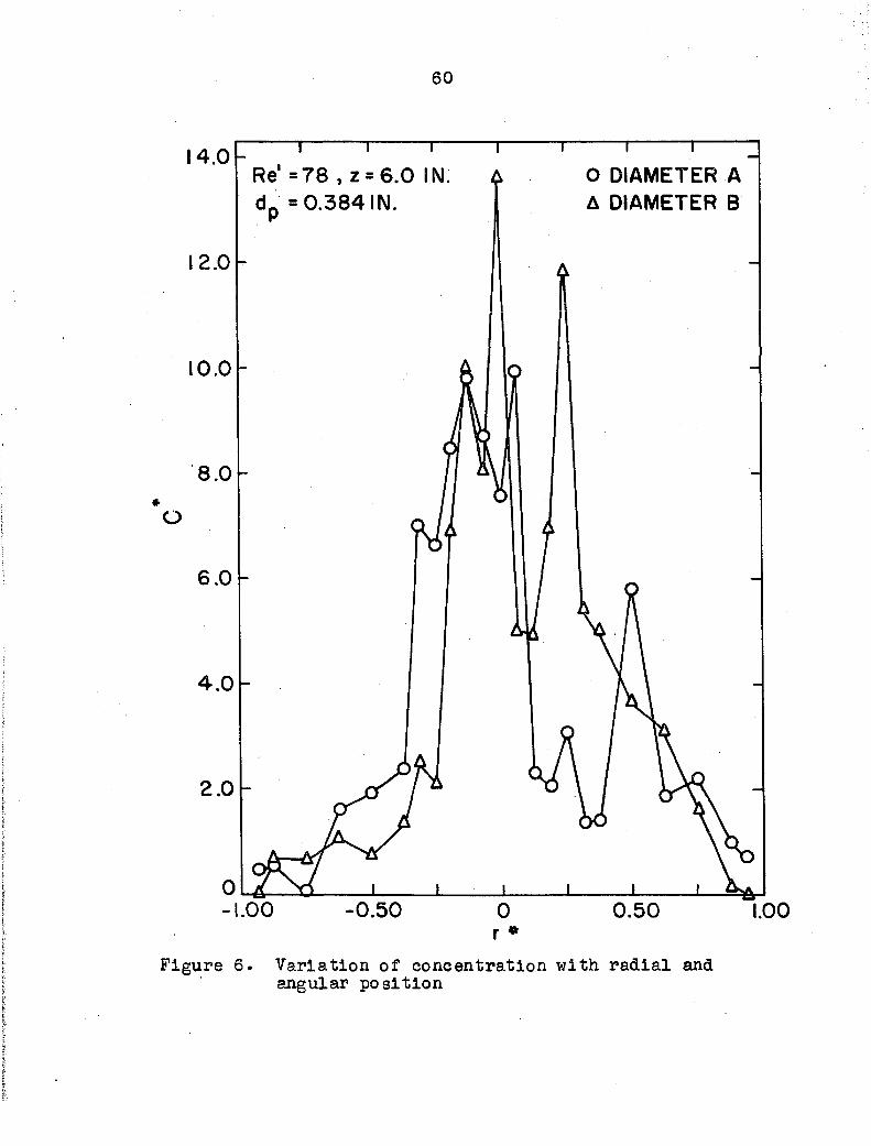
Later investigators (21, 24, 34) found that concentra­

tions in a packed bed varied not only from void to void but

also within an individual interstice. Concentrations of

samples removed from points on different radii but corre­

sponding to the same radial position were found to be dis­

tributed randomly about a mean concentration which may be

said to be characteristic of that radial position for the

59

particular experimental conditions. Preliminary experiments

of this investigation"yielded similar data. Figure 6 shows

the extent of these variations for two diameters 60 degrees

apart. Although these data were obtained when 0.384-inch

packing was in the column, similar results may be expected for

the 0.262-inch packing presently being considered.

Comparison of the concentration variations encountered in

this work with those reported by others (21, 24, 34) show that

the present variations are more extreme. This may be expected

because of the combined effects of the very small molecular

diffusion coefficient and the low flow rates investigated.

Fahien (24) concluded that concentration distributions

representative of the overall mass transfer process may be

obtained by averaging the concentrations from several equi­

angular positions for each radial position. A similar pro­

cedure was used in this study. However, in order to reduce

the time necessary to obtain the large number of individual

samples required, the multiple probe device was designed.

With this device one could simultaneously obtain samples for

several radial positions. In turn, the sample corresponding

to each radial position was a mixture of samples removed from

several angular positions. Concentration distributions

obtained in this manner could then be analyzed in terms of a

model assuming angular symmetry.

The reproducibility of concentration distributions

60

14.0 Re' = 78 , z = 6.0 IN. d- = 0.384 IN.

O DIAMETER A A DIAMETER B

12.0

10.0

8.0 -

O

6.0

4.0

2.0

-1.00 -0.50 0.50 1.00 0

r *

Figure 6. Variation of concentration with radial and angular position

61

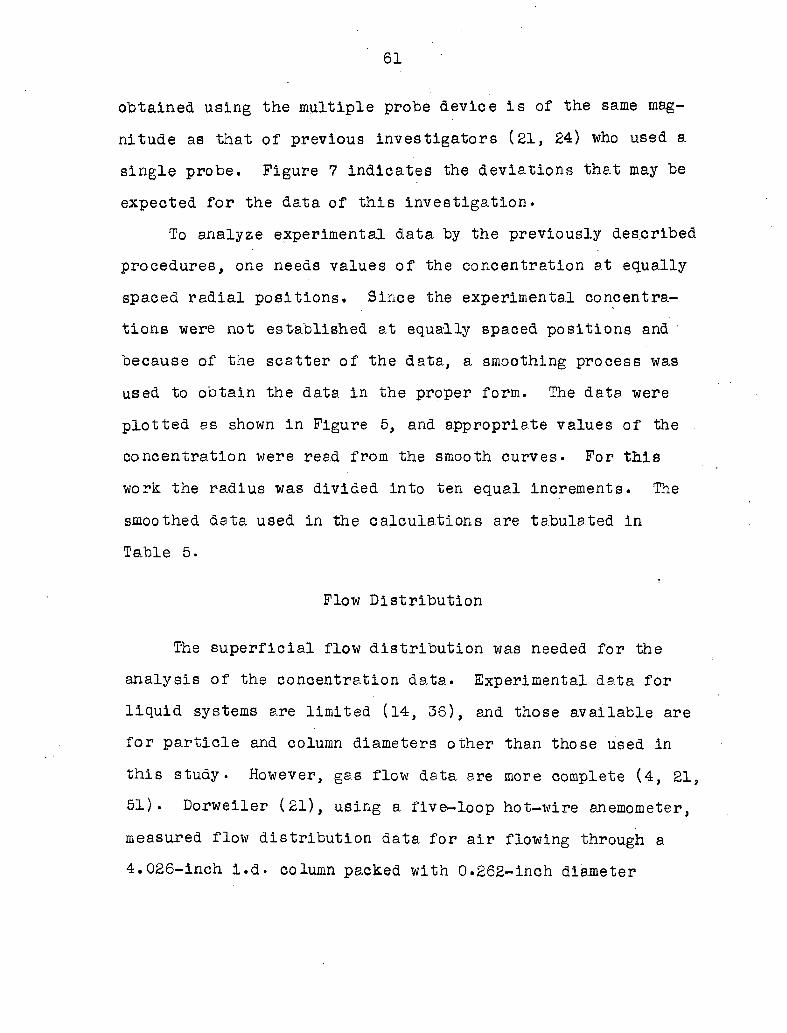
obtained using the multiple probe device is of the same mag­

nitude as that of previous investigators (21, 24) who used a

single probe. Figure 7 indicates the deviations that may be

expected for the data of this investigation.

To analyze experimental data by the previously described

procedures, one needs values of the concentration at equally

spaced radial positions. Since the experimental concentra­

tions were not established at equally spaced positions and

because of the scatter of the data, a smoothing process was

used to obtain the data in the proper form. The data were

plotted ss shown in Figure 5, and appropriate values of the

concentration were read from the smooth curves. For this

work, the radius was divided into ten equal increments. The

smoothed data used in the calculations are tabulated in

Table 5.

Flow Distribution

The superficial flow distribution was needed for the

analysis of the concentration data. Experimental data for

liquid systems are limited (14, 36), and those available are

for particle and column diameters other than those used in

this study. However, gas flow data are more complete (4, 21,

51). Dorweiler (21), using a five-loop hot-wire anemometer,

measured flow distribution data for air flowing through a

4.026-inch i.d- column packed with 0.262-inch diameter

62

8.0

Re'=7.1, z =23.0 IN.

O RUN 22F-3 A RUN 19A -0 • RUN 25F -2 X R U N 1 9 A - l © MEAN

7.0

ao

5.0

4.0 * o

3.0

2.0

02 0.4 0.6 0.8

Figure 7. Reproducibility of concentration distributions

63

pellets. He found that the flow distribution deviated sig­

nificantly from a uniform distribution and was essentially

independent of flow rate above a mean superficial velocity

of 0.4 foot per second (Re = 50). His data were used to

develop the flow distribution needed for this work. Such

usage assumes that the flow distributions for both gases and

liquids are identical under similar flow conditions.

Qualitatively, the flow distribution may be described

from considerations of the void fraction and the frictional

force exerted by the column wall on the fluid. If only void

fraction is considered (48, 50), the velocity distribution

would be nearly uniform in the central section of the column,

increasing on either side as the wall is approached. However,

the frictional force exerted by the wall causes the velocity

to decrease and thus approach a zero value right at the wall

surface. This concept is in general agreement with the

experimental data and is used herein to develop a quantitative

expression for the flow distribution.

One could plot the experimental data points and draw a

smooth curve through them. However, because only five points

were available, such a technique might result in assigning

unequal weight to each of the points. To avoid this possi­

bility the data were fitted to an empirical expression which

embodied the general concept outlined above. The expression

used was

64

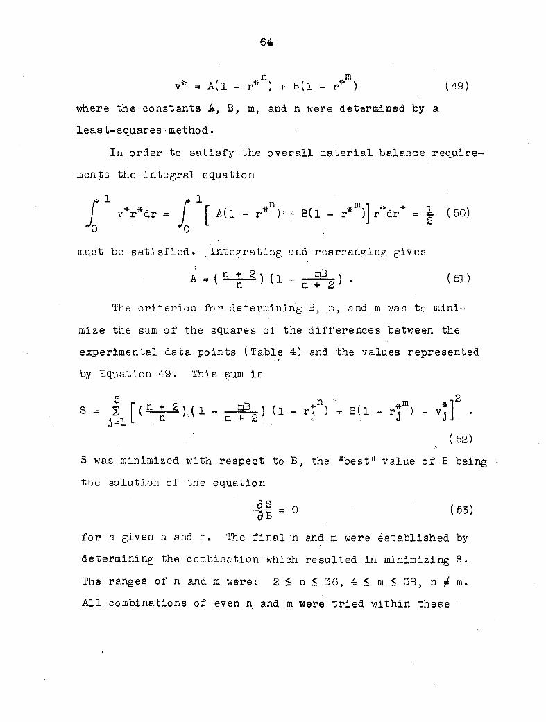
v* = A(1 - I-*") + B(1 - r*™) (49)

where the constants A, B, m, and n were determined by a

least-squares method.

In order to satisfy the overall material balance require­

ments the integral equation

j ~ v*r*dr = j £ A( 1 - r* ): + B( 1 - r* )] r*dr* = i- (50)

must be satisfied. . Integrating and rearranging gives

A .(Hi) (i - 5-aSg) • (si)

The criterion for determining B, n, and m was to mini­

mize the sum of the squares of the differences between the

experimental data points (Table 4) and the values represented

by Equation 49'. This sum is

s = A[ ( jL^ ,u u • r*n ' ; b ( i - r*m> -v*]8 • J--L

(52)

3 was minimized with respect to B, the "best" value of B being

the solution of the equation

-f|=0 (53)

for a given n and m. The final n and m were established by

determining the combination which resulted in minimizing S.

The ranges of n and m were: 2 < n < -36, 4 < m < 38, n / m.

All combinations of even n and m were tried within these '

65

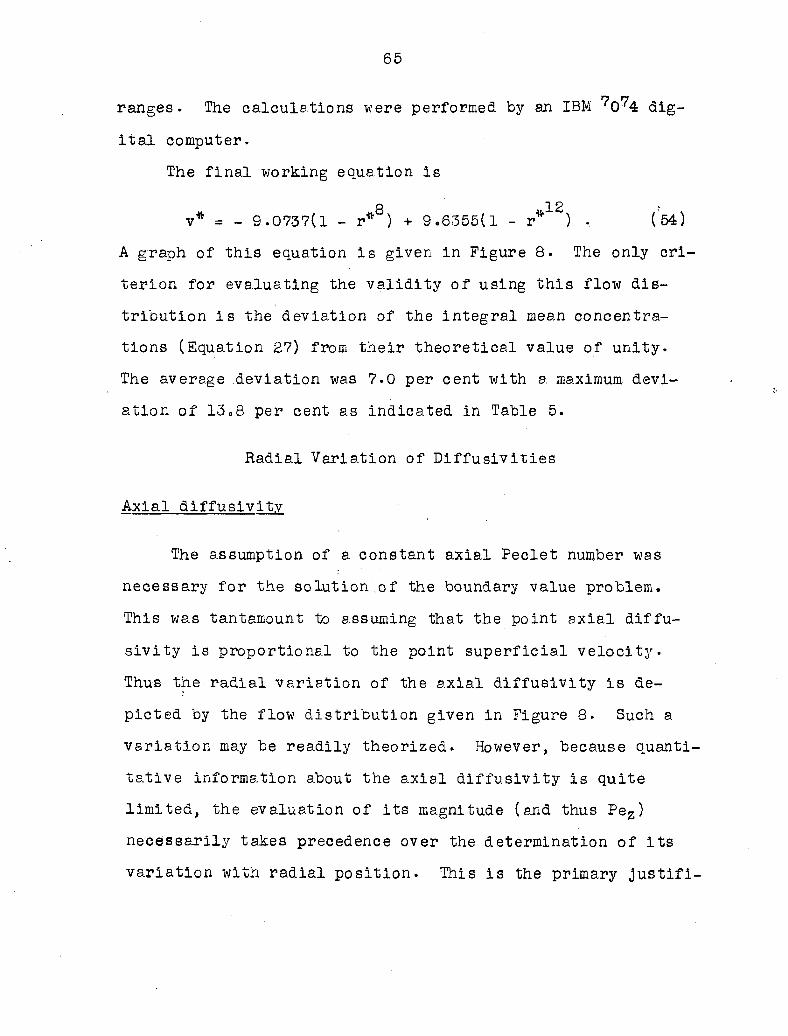
ranges. The calculations were performed by an IBM dig­

ital computer.

The final working equation is

8 12 v* = - 9.0737(1 - r* ) + 9.6355(1 - r* ) • (54)

A graph of this equation is given in Figure 8. The only cri­

terion for evaluating the validity of using this flow dis­

tribution is the deviation of the integral mean concentra­

tions (Equation 27) from their theoretical value of unity.

The average deviation was 7.0 per cent with a maximum devi­

ation of 13.8 per cent as indicated in Table 5.

Radial Variation of Diffusivities

Axial dlffuslvity

The assumption of a constant axial Peclet number was

necessary for the solution.of the boundary value problem.

This was tantamount to assuming that the point axial diffu-

sivity is proportional to the point superficial velocity.

Thus the radial variation of the axial diffusivity is de­

picted by the flow distribution given in Figure 8. Such a

variation may be readily theorized. However, because quanti­

tative information about the axial diffusivity is quite

limited, the evaluation of its magnitude (and thus Pez)

necessarily takes precedence over the determination of its

variation with radial position. This is the primary justifi-

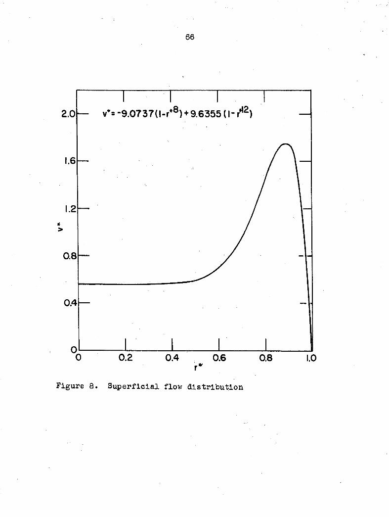
66

-9.0737(l-r*°) + 9.6355 (hf*) 2.0

1.6

0.8

0.4

0.2 0.4 0.6 0.8

Figure 8. Superficial flow distribution

67

cation for assuming a constant axial Peclet number in this

study.

Radial diffusivity

The variation of the radial diffusivity with radial posi­

tion is shown in Figure 9. This variation was established

from calculations (Appendix A) in which the smoothed concen­

tration data for the following conditions were used: Re1 =

84.9, z = -32.0 inches. These data satisfied the requirement

that they could be accurately described by Equation 33.

The variation of p given in Figure 9 was used for the

entire flow rate range. Fahien (24) found that for the carbon

dioxide-air system the radial variation of the radial diffu­

sivity was independent of flow rate. Dorweiler and Fahien

(22) later showed that the variation was not independent of

flow rate for rates corresponding to Reynolds number below

approximately 100. This dependency exists as a result of the

increasing molecular contribution to the overall transfer

process at low Reynolds numbers. Since the molecular diffu­

sion coefficient for liquids is on the order of one ten-

thousandth of that for gases, such a dependency may be ex­

pected in liquid systems only at much lower Reynolds numbers.

It is interesting to compare the variation of the radial

diffusivities with radial position for gases and liquids.

Both Fahien (24) and Dorweiler (21) found greater variations

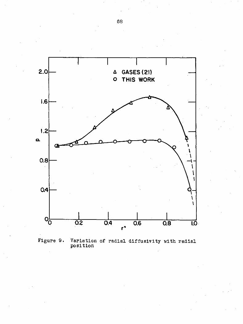
68

2.0 A GASES (21) O THIS WORK

1.6

O.

0.8 -t-

0.4

0.2 0.4 0.6 0.8 1.0

Figure 9. Variation of radial diffusivity with radial position

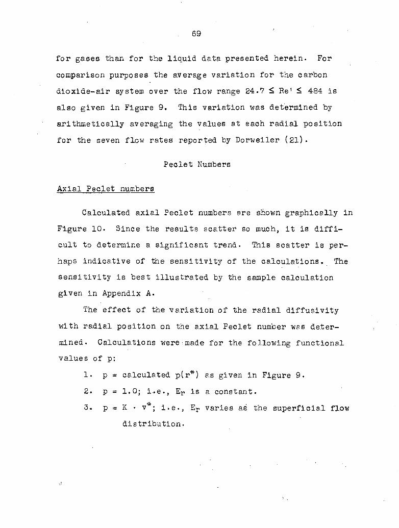
69

for gases than for the liquid data presented herein. For

comparison purposes the average variation for the carbon

dioxide-air system over the flow range 24.7 < Re1 5 484 is

also given in Figure 9. This variation was determined by

arithmetically averaging the values at each radial position

for the seven flow rates reported by Dorweiler (21).

Peclet Numbers

Axial Peclet numbers

Calculated axial Peclet numbers are shown graphically in

Figure 10. Since the results scatter so much, it is diffi­

cult to determine a significant trend. This scatter is per­

haps indicative of the sensitivity of the calculations. The

sensitivity is best illustrated by the sample calculation

given in Appendix A.

The effect of the variation of the radial diffusivity

with radial position on the axial Peclet number was deter­

mined . Calculations were-made for the following functional

values of p:

1. p = calculated p(r*) as given in Figure 9.

2. p = 1.0; i.e., Er is a constant.

•3. p = K • v*; i.e., Er varies as the superficial flow

distribution.

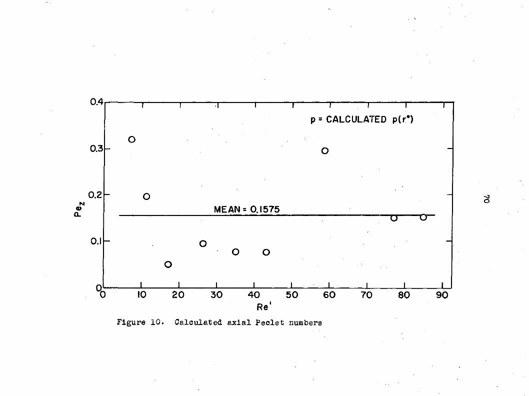
1 1 1 1 1 II 1

p = CALCULATED p(r*)

!"

o -

O —

o

MEAN = 0.1575

—

u û

o

O O O

1 1 1 I 1 1 1 1 1 0 10 20 30 40 50 60 70 80 90

Re'

Figure 10. Calculated axial Peclet numbers

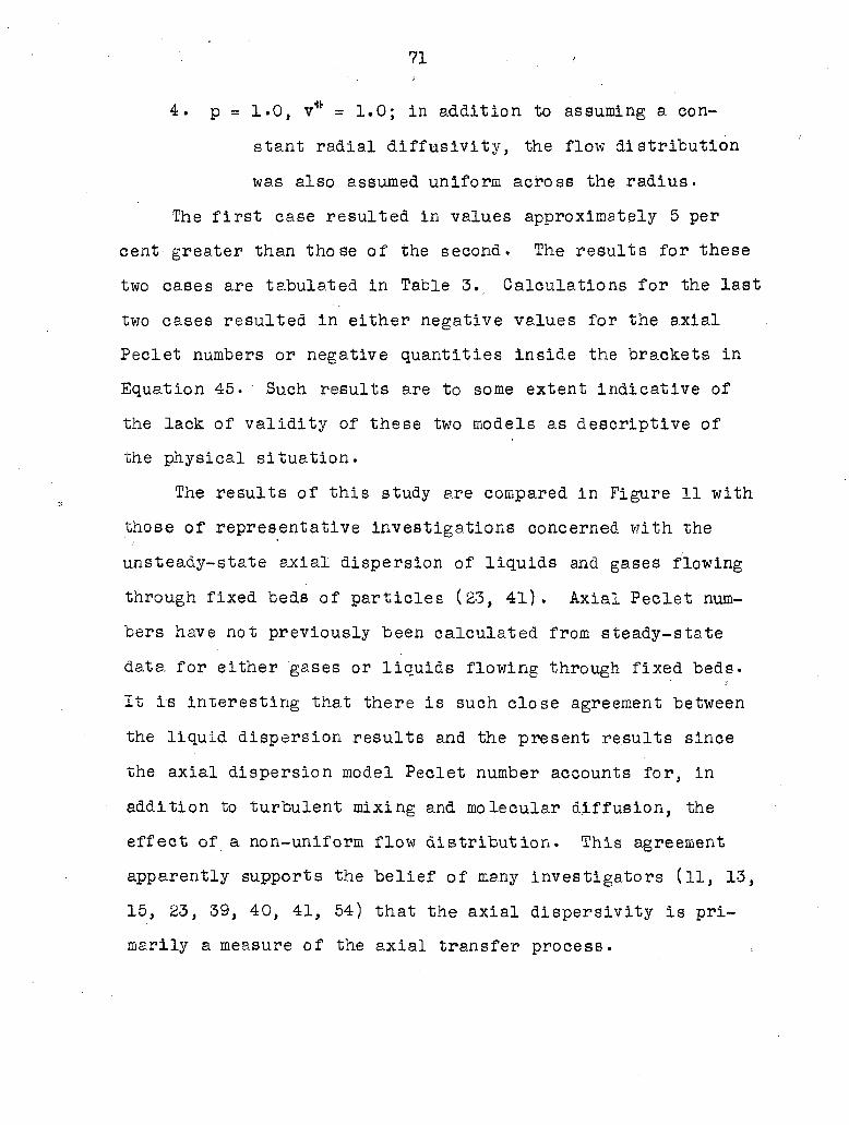
71

4. p = 1.0, v* = 1.0; In addition to assuming a con­

stant radial diffusivity, the flow distribution

was also assumed uniform across the radius•

The first case resulted in values approximately 5 per

cent greater than those of the second. The results for these

two cases are tabulated in Table 3. Calculations for the last

two cases resulted in either negative values for the axial

Peclet numbers or negative quantities inside the brackets in

Equation 45. ' Such results are to some extent indicative of

the lack of validity of these two models as descriptive of

the physical situation.

The results of this study are compared in Figure 11 with

those of representative investigations concerned with the

unsteady-state axial dispersion of liquids and gases flowing

through fixed beds of particles (23, 41). Axial Peclet num­

bers have not previously been calculated from steady-state

data for either gases or liquids flowing through fixed beds.

It is interesting that there is such close agreement between

the liquid dispersion results and the present results since

the axial dispersion model Peclet number accounts for, in

addition to turbulent mixing and molecular diffusion, the

effect of a non-uniform flow distribution. This agreement

apparently supports the belief of many investigators (11, 13,

15, 23, 39, 40, 41, 54) that the axial dispersivity is pri­

marily a measure of the axial transfer process.

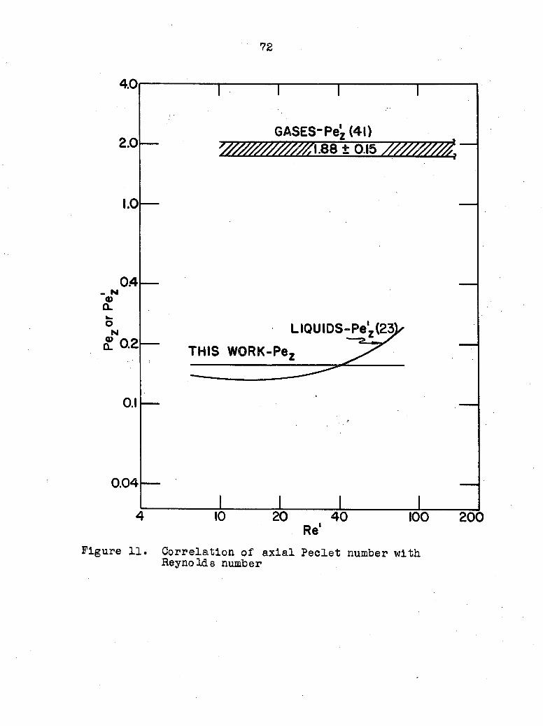
72

1.0

- N Q> cl fc . O N

5Î 0.2

0.04

GÂSES-Pe'z (41) ^̂ ,̂.88 ± 015

LIQUIDS-Pe

THIS WORK-Pe,

10 1

20 40 Re*

1 100 200

Figure 11. Correlation of axial Peclet number with Reynolds number

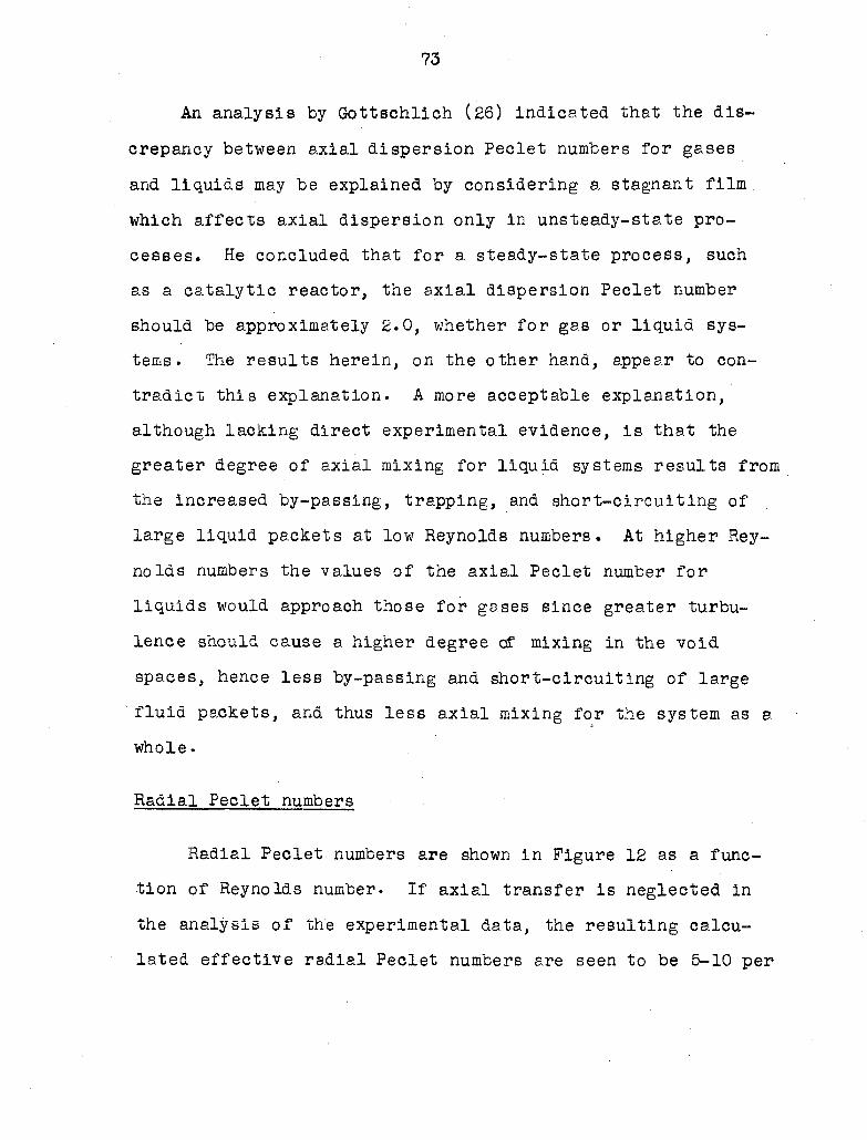
73

An analysis by Gottschlich (26) indicated that the dis­

crepancy between axial dispersion Peclet numbers for gases

and liquids may be explained by considering a stagnant film

which affects axial dispersion only in unsteady-state pro­

cesses. He concluded that for a steady-state process, such

as a catalytic reactor, the axial dispersion Peclet number

should be approximately 2.0, whether for gas or liquid sys­

tems. The results herein, on the other hand, appear to con­

tradict this explanation. A more acceptable explanation,

although lacking direct experimental evidence, is that the

greater degree of axial mixing for liquid systems results from

the increased by-passing, trapping, and short-circuiting of

large liquid packets at low Reynolds numbers. At higher Rey­

nolds numbers the values of the axial Peclet number for

liquids would approach those for gases since greater turbu­

lence should cause a higher degree of mixing in the void

spaces, hence less by-passing and short-circuiting of large

fluid packets, and thus less axial mixing for the system as a

whole.

Radial Peclet numbers

Radial Peclet numbers are shown in Figure 12 as a func­

tion of Reynolds number. If axial transfer is neglected in

the analysis of the experimental data, the resulting calcu­

lated effective radial Peclet numbers are seen to be 5-10 per

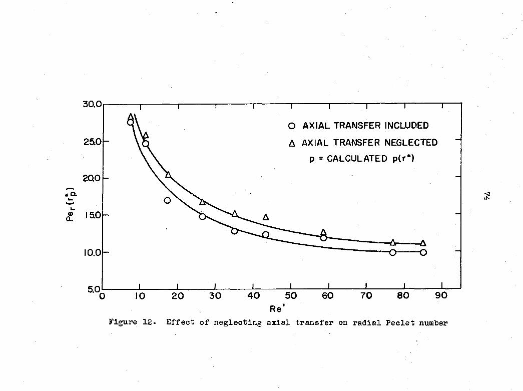
1 1 I 1

O AXIAL TRANSFER INCLUDED

A AXIAL TRANSFER NEGLECTED

p = CALCULATED p(r* )

•A

10 20 30 40 50 60 70 80 90 Re '

Figure 12. Effect of neglecting axial transfer on radial Peclet number

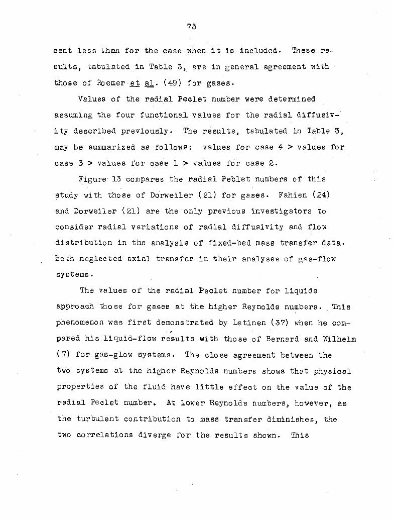
75

cent less than for the case when it is included. These re­

sults, tabulated in Table -3, are in general agreement with

those of Roemer e_t al. (49) for gases.

Values of the radial Peclet number were determined

assuming the four functional values for the radial diffusiv-

ity described previously. The results, tabulated in Table 3,

may be summarized as follows: values for case 4 > values for

case 3 > values for case 1 > values for case 2.

Figure 13 compares the radial Peclet numbers of this

study with those of Dorweiler (21) for gases. Fabien (24)

and Dorweiler (21) are the only previous investigators to

consider radial variations of radial diffusivity and flow

distribution in the analysis of fixed-bed mass transfer data.

Both neglected axial transfer in their analyses of g as-flow-

systems .

The values of the radial Peclet number for liquids

approach those for gases at the higher Reynolds numbers. This

phenomenon was first demonstrated by Latinen (37) when he com­

pared his liquid-flow results with those of Bernard and Wilhelm

(7) for gas-glow systems. The close agreement between the

two systems at the higher Reynolds numbers shows that physical

properties of the fluid have little effect on the value of the

radial Peclet number. At lower Reynolds numbers, however, as

the turbulent contribution to mass transfer diminishes, the

two correlations diverge for the results shown. This

80-

60 —

40-

* û.'

£

20-

10

8

6 —

T AXIAL TRANSFER NEGLECTED

p FROM FIGURE 9

1 1 1

6 8 10 1 20

OTHIS WORK"rp =0.05

A GASES (2l)-rp*=0.0625

ir

I I I L I 1 1 1

200 400 600 800 40 60 80100 Re

Figure 13. Correlation of radial Peclet number with Reynolds number

m

77

divergence arises because the molecular diffusion coefficient

for gases is on the order of ten thousand times greater than

that for liquids. The gas-flow radial Peclet number reaches

a maximum and then decreases with Reynolds number as the

turbulent effect damps out, ultimately reaching a linear

relationship with Reynolds number. One may expect a similar

effect in the liquid-flow correlation, although at a much

lower flow rate.

Prediction of Concentration Distributions

One test of the validity of mass transfer models is to

compare the predicted concentration distributions for each

model with those of others and with experimental data. Pre­

dicted concentration distributions for the diffusivity models

previously described are compared graphically in Figures 14

through 18. Figure 20 illustrates the agreement between the

diffusivity model and a two-dimensional finite stage model.

Comparison of diffusivity models

Figures 14 and 15 show the effect of neglecting axial

transfer on the prediction of concentration distributions.

The infinite axial Peclet number represents the case when

axial transfer is neglected. Except for the central portion

of the distributions the effect is quite small. Even the

discrepancy near the center is not large ( ~ 10 per cent).

78

6.0 Re'=7.|, 2 = 32.0 IN.

5.0

g

— •

4.0

° 3.0

2,0

1.0

0

Figure 14,

g

S3

ps CALCULATED p(r*)

OPer(r*p)= 27.5822

Pez =0.3214

APer (r*)=28.l93l

Pez = ®

D EXPERIMENTAL DATA

Ô

Ô

Ô

§

© • ©

0.2 • é

0.4 0.6 0.8 1.0

Effect of neglecting axial transfer on concentration distribution

79

Re'=84.9,z=l5.5IN. p= CALCULATED p(r')

OPer(rg)= 9.8862

A

•e o

o A

Pez=O.I529

O A Rer (rp«l 1.0587

Pe£=co

DEXPERIMENTAL DATA

%

&

A O

0 A O

6

d°

8 • 8 0.2 0.4 r 0.6 0.8 1.0

Figure 15. Effect of neglecting axial transfer on concentration distribution

80

The larger discrepancy near the center becomes quite accept­

able when one realizes that the flow in the central portion

of the bed is a very small fraction of the total flow. For

example, the flow in the portion of the bed represented by

0 < r* < 0.3 is approximately 5 per cent of the total flow;

i.e.,

.0.3

f v*r*dr*

" = 0.05 . (55)

v*r*dr*

Although axial transfer is seen to be of little importance in

this study, even at very low flow rates, one may not neces­

sarily neglect it when designing chemically reactive systems

in which axial concentration gradients may be extremely large.

Figures 16 and 17 show the deviations between predicted

concentration distributions for the calculated radial vari­

ation of the radial diffusivity and for a constant radial

diffusivity. The small deviations (generally less than 1 per

cent) should perhaps be expected since the calculated diffu­

sivity variation is not very great across most of the radius

as shown in Figure 9.

Figure 18 summarizes the effects of the four radial

diffusivity models described previously on the prediction of

concentration distributions• A cursory inspection indicates

that all four models may be acceptable• However, here the

/

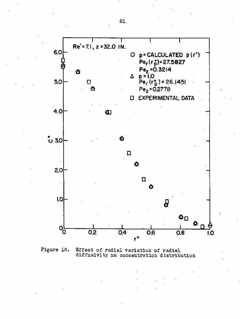
81

I 1 1 1

Re.'87.1, z =32.0 IN. 60J~ O p = CALCULATED p(r*)

Per (rp)= 27.5827 Q Pez =0.3214

A p = 1.0 5.01- D Per(r*p) = 26,145!

Û Pez =0.2778

0 EXPERIMENTAL DATA

4.0h Q]

o3i0

ao

1.0

0

Ô

•

Û

• o

8

6 o_£

0 02 0.4 0.6 0.8 1.0 r*

Figure 16. Effect of radial variation of radial diffusivity on concentration distribution

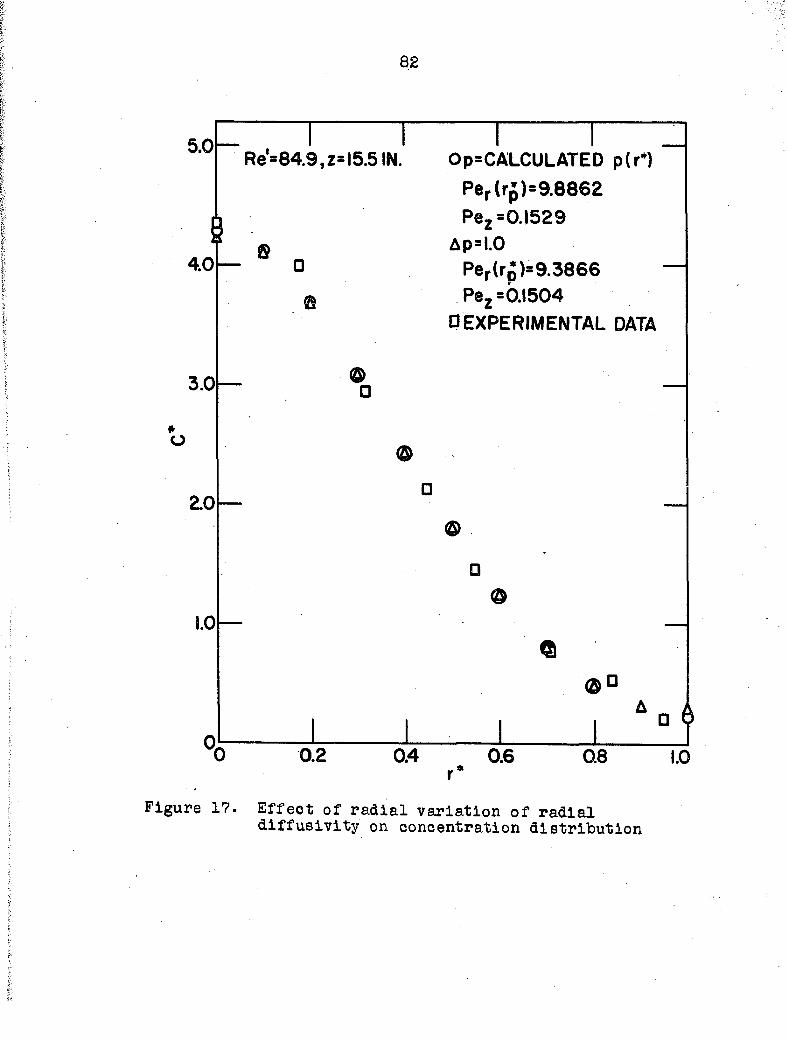
82

5.0 Re'=84.9,z=l5.5 IN. Op=CALCULATED p(r*)

Per(rp)=9.8862

Pez =0.1529

fi Ap=I.O — •

* o

2.0

Per(r£)=9.3866 Pez =0.1504

D EXPERIMENTAL DATA

•

©

Figure 17. Effect of radial variation of radial diffusivity on concentration distribution

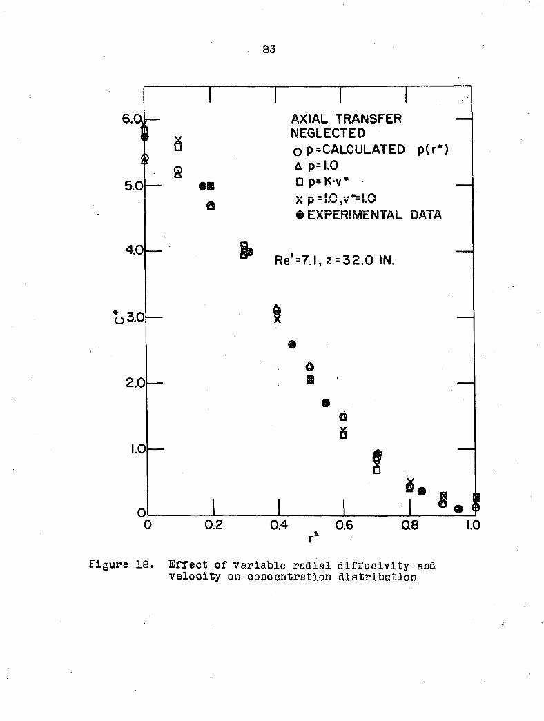
83

6V H

5.0

4.0

o 3.0

2.0

1.0

S

»

0.2

AXIAL TRANSFER NEGLECTED OP CALCULATED p(r*) A p= 1.0 • p= K-v* X p = !.0,v*=!.0 # EXPERIMENTAL DATA

Re'=7.1, 2 = 32.0 IN.

I

Ô B

O

8

& 8

0.4 0.6 0.8 1.0

Figure 18. Effect of variable radial diffusivity and velocity on concentration distribution

84

graphical test of the models must be supplemented. First,

the assumption of a uniform flow distribution in case 4 does

not result in acceptable material balances; i.e., the calcu­

lated values of 0^ are in very poor agreement with the theo­

retical value of unity (Table 5). Second, for cases 3 and 4

no axial Peclet number could be calculated. It is true that

for this work axial transfer appears to be of little impor­

tance. However, the practical value of this study lies in the

utility of the various mass transport parameters for design­

ing chemical engineering equipment, and in particular, equip­

ment for chemically reactive systems. The importance of con­

sidering axial transfer in these systems has not been fully

established. And finally, Richardson (46), in a recent study,

showed that case 1 resulted in the best agreement between

experimental and calculated mean conversions for the oxidation

of sulfur dioxide in a fixed-bed catalytic reactor. The next

best agreement was obtained for case 4 and the poorest agree­

ment was obtained for case 3.

Comparison of diffusivity and finite stage models

Deans and Lapidus (18) developed a mathematical model

for predicting the mixing characteristics of fixed beds of

spheres. The model is based on a two-dimensional network of

perfectly mixed stages.. A material balance about a general

stage provides a working equation for determining the concen­

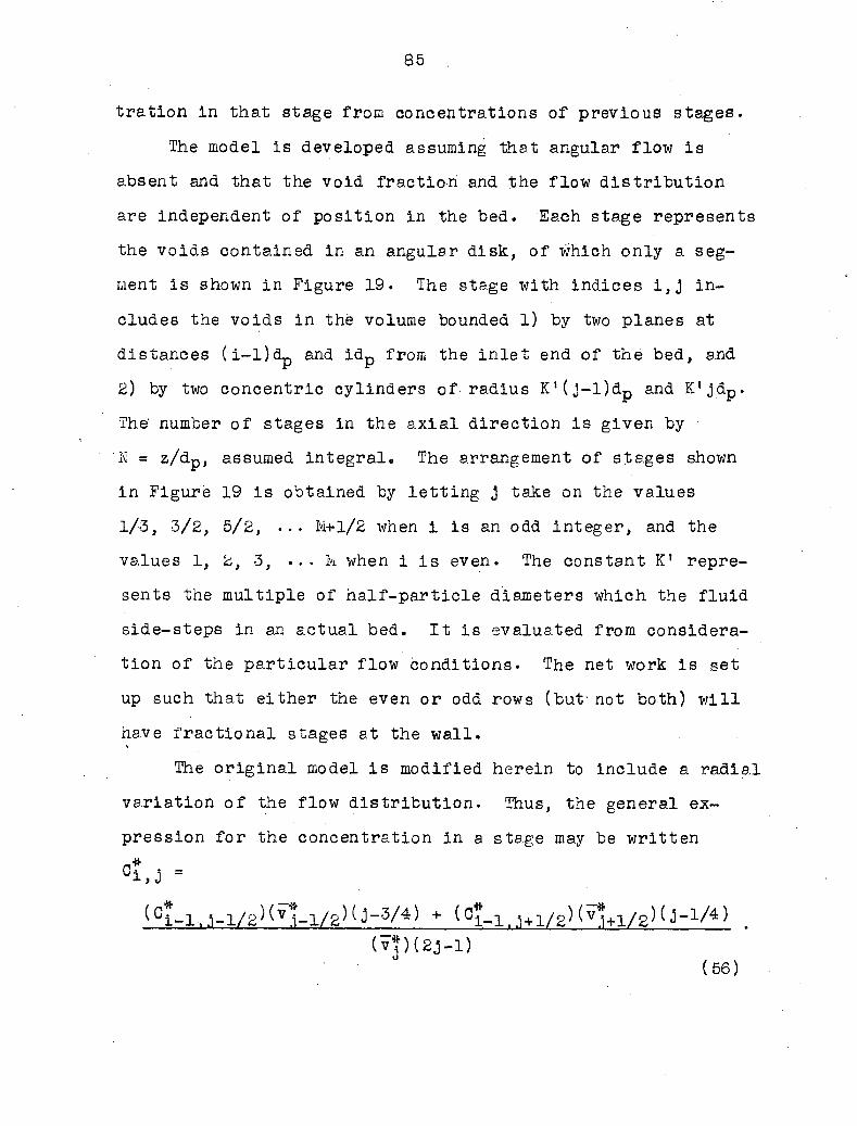
85

tration in that stage from concentrations of previous stages.

The model is developed assuming that angular flow is

absent and that the void fraction and the flow distribution

are independent of position in the bed. Each stage represents

the voids contained in an angular disk, of which only a seg­

ment is shown in Figure 19. The stage with indices i,j in­

cludes the voids in the volume bounded l) by two planes at

distances (i-l)dp and idp from the inlet end of the bed, and

2) by two concentric cylinders of radius K'(j-l)dp and K'jdp.

The' number of stages in the axial direction is given by

N = z/dp, assumed Integral. The arrangement of stages shown

in Figure 19 is obtained by letting j take on the values

1/3, 3/2, 5/2, ... M+l/2 when i is an odd integer, and the

values 1, 2, 3, ... M when i is even. The constant K1 repre­

sents the multiple of half-particle diameters which the fluid

side-steps in an actual bed. It is evaluated from considera­

tion of the particular flow conditions. The net work is set

up such that either the even or odd rows (but not both) will

have fractional stages at the wall.

The original model is modified herein to include a radial

variation of the flow distribution. Thus, the general ex­

pression for the concentration in a stage may be written

°i,J =

tCl-l, .1-1/2^v*-1/SHJ-5/4) + (C*-l. j+l/g) (Vj+l/2)(J-l/4) e

(v?)(2j_l)

(56)

86

Figure 19. Schematic representation of the arrangement of stages for the finite stage mass transfer model

87

From Figure 17 it is easily seen that the flow through a given

stage is the sum of partial flows from each of the two preced­

ing stages. In order that the total flow be conserved, it is

necessary to accurately define the mean dlmensionless vel­

ocities in Equation 56. This is done mathematically by the

following expressions:

I 4-1/2

v*r*dr*

**-1/2 " y (5?) ="3-1/2 *

/ r "dr

rj-l

L v*r*dr*

(58) j

r*dr*

i-i/2

/. 4+1/2

v*r*dr*

^ (59)

fj+1/2

/ v*r*dr*

4-1/2

88

For the particular case j = 1/2 it is easily seen from Figure

17 that

°i,1/2 = Ci-l,l ' (GO)

If the radius is divided into an Integral number of stage

widths, the equation for the fractional stage at the wall is

seen to be

°i,M+l/2 = °i=l,M ' (61)

Simulation of the experimental system.used in this study

was readily accomplished by the use of the finite stage model.

The steady-state concentrations of all stages in an arbitrary

network are given by Equations 56, 60, and 61. The only -

external condition required is the stipulation of the tracer

concentration in the inlet stream, which is given by

°1,1/2 = 4 (62)

where q is arbitrary. For comparison purposes q was chosen

such that Cj4 was unity. Mathematically,

Cm J v*r*dr*

q = 5 (63) rj=l/2

v*r*dr*

0

Other parameters chosen were M = 8 and M = 271. The value of

M was calculated from the relation

/

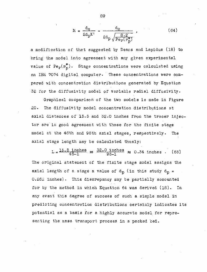
89

M = -âa_ „ a° , (64)

a modification of that suggested by Deans and Lap!dus (18) to

bring the model into agreement with any given experimental

value of Per(rp). Stage concentrations were calculated using

an IBM 7074 digital computer. These concentrations were com­

pared with concentration distributions generated by Equation

32 for the diffusivity model of variable radial diffusivity.

Graphical comparison of the two models is made in Figure

20. The diffusivity model concentration distributions at

axial distances of 15.5 and 32.0 inches from the tracer injec­

tor are in good agreement with those for the finite stage

model at the 46th and 95th axial stages, respectively. The

axial stage length may be calculated thusly:

L = 15*6_lBShes y 3S.Clinches w 0-34 lnches . (66)

The original statement of the finite stage model assigns the

axial length of a stage a value of dp (in this study dp =

0.262 inches). This discrepancy may be partially accounted

for by the method in which Equation 64 was derived (18). In

any event this degree of success of such a simple model in

predicting concentration distributions certainly indicates its

potential as a basis for a highly accurate model for repre­

senting the mass transport process in a packed bed.

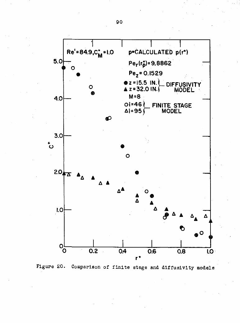
90

Re'=84.9,0^ = 1.0

o o

o

p=GALCULATED p(r*)

Per(rJ)=9.8862

Pez= 0.1529

• z = 55.5 IN.L DIFFUSIVITY â z = 32.0 IN.j MODEL

M=8

Ols46) FINITE STAGE Ai = 95) MODEL

* o

2.0 ' T A A A

A A

A s O A # A

A A _ < r * 4 a a »

t>

0 0.2 0.4 0.6 0.8 1.0 r*

Figure 20. Comparison of finite stage and diffusivity models

91

SUMMARY AND CONCLUSIONS

The major results of this study may be summarized as

follows:

1. Concentration distributions were measured for a

tracer material being transported in a main stream of water

flowing slowly (Re1 < 100) through a packed bed of spherical

particles.

2» Axial and radial Peclet numbers were determined from

the data of a single experiment.

3̂ . Values of the axial Peclet number were found to be

on the order of one-hundredth those of the radial Peclet

number; hence, the axial diffusivity is approximately one

hundred times greater than the radial diffusivity for the

conditions of this investigation.

4. Although the axial diffusivity was found to be much

larger than the radial diffusivity, the effect of including

axial transfer in the prediction of concentration distribu­

tions was shown to be quite small. However, for chemically

reactive systems, in which large axial concentration gradi­

ents may exist, axial transport may be significant.

5. The variation of the radial diffusivity with radial

position was found to be much less pronounced than that for

gas-flow systems as determined by previous investigators.

6. The empirical equation used to correlate flow dis­

tribution data for gases appears to adequately represent the

92

flow distribution for liquids in fixed beds of identical

physical configuration. The sole basis for this conclusion

is the good agreement between the calculated integral mean

concentrations and their theoretical value of unity.

93

NOMENCLATURE

constant in flow distribution equation

matrix notation used in numerical solution of Sturm-Liouville problem

constant in series solution

constant in flow distribution equation

modified constant in series solution

matrix notation used in numerical solution of Sturm-Liouville problem

concentration of transferring material

measured steady-state mean concentration in the column

dlmensionless concentration, C/Cg

dlmensionless concentration of tracer material

dlmensionless concentration in the i,j stage of finite stage model

integral mean concentration, defined by Equation 27

molecular diffusion coefficient

matrix notation used in numerical solution of Sturm-Liouville problem

total effective axial "diffusivity11 or dispersivity

differential operator

column diameter

mean packing diameter

dlmensionless particle diameter, dp/r0

effective diffusivity, a scalar quantity

component in total diffusivity tensor; i = r,jzf, z : j = r>,z

94

Er radial diffusivity, Err

Er(rp) radial diffusivity evaluated at rp,

Eti1 component in turbulent diffusivity tensor; i = r,gf,z; j =

Ez axial diffusivity, Ezz

E total diffusivity tensor

Et turbulent diffusivity tensor

h dlmensionless radial increment length, 1/N

I unit matrix

I unit second-order tensor

1 designation of axial position of stage in finite stage model

J mass transfer flux vector

j designation of radial position of stage in finite stage model; summation index

K proportionality constant

K1 multiple' of half-particle diameters which the fluid side-steps in an actual bed

k point of division in dlmensionless radius, k = 0, 1, .. . N

L axial length of stage in finite stage model

M whole number of stages across radius in finite stage model

m correlation function; subscript indicating an arbi­trary elgen function; exponent in flow distribution equation

N total number of increments of division in 0 < r*< 1.0; number of stages in axial direction in finite stage model

n subscript indicating an arbitrary eigen value and its corresponding eigen function; exponent in flow dis­tribution equation; correlation function

95

Pe general Peclet number, dpV/E

Per(r^) radial Peclet number evaluated at rp, dpuz(rp)/Er(rp)

Pez axial Peclet number, dpuz(r)/Ez(r)

Pez axial Peclet number, dpV/D^

Pez axial Peclet number, dpU/D^

p radial variation of Er, Er(r)/Er(rp)

Q,n symbol for expression given in Equation 45

q dlmensionless tracer concentration in the inlet stream of the finite stage model

R solution to Sturm-Liouville problem

Re' Reynolds number, dpV/( fx / p )

Re11 line Reynolds number, d'pV/e { f x / p )

Rn(k) eigen function

r radial coordinate; radial distance from center of packed column

r^ radius of injection tube

rQ radius of column

rp a specified radial position

r* dlmensionless radial position, r/r0

r* dlmensionless radius of injection tube, rj_/r0

r* dlmensionless rp, rp/r0

S symbol for sum given in Equation 52

Tg measured mean temperature of effluent stream

t time

U mean interstitial velocity, V/e

uz axial component of superficial velocity vector

96

superficial velocity vector

mean superficial velocity, based on empty column cross section

dlmensionless flow distribution, u2(r)/V

dlmensionless flow distribution evaluated at rp

mean dlmensionless velocity defined by Equations 57, 58, and 59

particular solution of Equation 12

axial coordinate; axial distance from tracer injection tube

dlmensionless axial position, z/ro

large dlmensionless axial distance from the injection tube

small dlmensionless axial distance from the injection tube

a real positive number

eigen value

gradient operator

partial differential operator

mean void fraction in packed column

fluid kinematic viscosity

summation symbol

angular coordinate

integration symbol

97

LITERATURE CITED

I. Aris, R. On the dispersion of a solute in a fluid flow­ing through a tube. Royal Society of London Proceedings Series A, 2-35:67-77. 1956.

2• Aris, R. Notes on the diffusion-type model for longi­tudinal mixing in flow: letter to the editors. Chemical Engineering Science 9:266-267. 19 59.

3. Aris, R. and Amundson, N. R. Some remarks on longi­tudinal mixing or diffusion in fixed beds. American Institute of Chemical Engineers' Journal 3:280-282• 1957.

4. Arthur, J. R., Linnett, J. W., Raynor, E. J., and Sington, E. P. C. The flow of an air stream through a layer of granules. Faraday Society Transactions 46: 270-281. 1950.

5. Baron, T. Generalized graphical method for the design of fixed-bed catalytic reactors. Chemical Engineering Progress 48:118-124. 1952.

6. Beek, J. Design of packed catalytic reactors. Advances in Chemical Engineering 3:203-271. 1962.

7. Bernard, R. A. and Wilhelm, R. H. Turbulent diffusion in fixed beds of packed solids. Chemical Engineering Progress 46:233-244. 1950.

8. Bischoff, K. B. Notes on the diffusion-type model for longitudinal mixing in flew: letter to the editors. Chemical Engineering Science 12:69-70. 1960.

9. Bisçhoff, K. B. and Levenspiel, 0. Fluid dispersion. I. Generalization of models. Chemical Engineering Science 17:245-255. 1962.

10. Bischoff, K. B. and Levenspiel, 0. Fluid dispersion. II. Comparison of models. Chemical Engineering Science 17:257-264. 1962.

II. Bradshaw, R. D. and Bennett, C. 0. Fluid-particle mass transfer in a packed bed. American Institute of Chemical Engineers'- Journal 7:48-52. 1961.

98

12. Cairns, E. J. and Prausnitz, J. M. Longitudinal mixing in fluidization. American Institute of Chemical Engi­neers' Journal 6:400-405. 196.0.

13. Cairns, E. J. and Prausnitz, J. M. Longitudinal mixing in packed beds• Chemical Engineering Science 12:20-34. 1960.

14. Cairns, E. J. and Prausnitz, J. M. Velocity profiles in packed and fluidized beds. Industrial and Engineering Chemistry 51:1441-1444. 1959.

15. Carberry, J. J. and Bretton, R. H. Axial dispersion of mass in flow through fixed beds. American Institute of Chemical Engineers' Journal 4:367-375. 1958.

16. Converse, A. 0. The effect of velocity profile on axial dispersion in packed beds. American Institute of Chemi­cal Engineers' Journal 6:344-345. 1960.

17. Danckwerts, P. V. Continuous flow systems ; distribution of residence times. Chemical Engineering Science 2: 1-13. 1953.

18. Deans, H. A. and Lapidus, L. A computational model for predicting and correlating the behavior of fixed-bed reactors. I. Derivation of model for nonreactive systems. American Institute of Chemical Engineers' Journal 6:656-663• 1960.

19. Deans, H. A. and Lapidus, L. A computational model for predicting and correlating the behavior of fixed-bed reactors. II. Extension to chemically reactive systems. American Institute of Chemical Engineers' Journal 6: 663-668. I960.

20. Deisler, P. F. and Wilhelm, R- H. Diffusion in beds of porous solids. Industrial and Engineering Chemistry 45: 1219-1225. 1953.

21. Dorweiler, V. P. Mass transfer at low flow rates in a packed column. Unpublished M.S. thesis. Ames, Iowa, Library, Iowa State University of Science and Technology. 1956.

22. Dorweiler, V. P. and Fahien, R. W. Mass transfer at low flow rates in a packed column. American Institute of Chemical Engineers' Journal 5:139-144 . 19 59.

99

23. Ebach, E. A. and White, R. R. Mixing of fluids flowing through beds of packed solids. American Institute of Chemical Engineers' Journal 4:161-169. 1958.

24. Fahien, R. W. Mass transfer in packed beds. Unpublished Ph.D. thesis- Lafayette, Indiana, Library, Purdue Uni­versity. 1954.

25. Fahien, R. VI. and Smith, J. M. Mass transfer in packed beds. American Institute of Chemical Engineers' Journal

. 1:28-37. 1955.

26. G-ottschlich, G. F. Axial dispersion in a packed bed. American Institute of Chemical Engineers' Journal 9: 88-92. 1963.

27. Hanratty, T. J., Latinen, G-., arid Wilhelm, R. H. Turbu­lent diffusion in perticulately fluidized beds of par­ticles. American Institute of Chemical Engineers' Journal 2:372-380. 1956.

28. Hennico, A., Jacques, G., and Vermeulen, T. Longitudinal dispersion in packed extraction columns. University of California Radiation Laboratory Report 10696. 1963.

29. Hiby, J. W. and Schummer, P. Zur Messung der trans-versalen effektiven Diffusion iri durchstromten Fill 11-korpers&ulen. Chemical Engineering Science 13:69-74. 1960.

30. Houston, R. H. A theory for industrial gas-liquid chroma­tographic columns. University of California Radiation Laboratory Report 3817. 1958.

31. Jacques, G. L. and Vermeulen, T. Longitudinal dispersion in solvent-extraction columns; Peclet numbers for ordered and random packings. University of California Radiation Laboratory Report 8029. 1957.

32. Klinkenberg, A., Krajenbrink, H. J., and Lauwerier, H. A. Diffusion in a fluid moving at uniform velocity in a tube. Industrial and Engineering Chemistry 45:1202-1208. 1953.

33. Kramers, H. and Alberda, G. Frequency response analysis of continuous flow systems. Chemical Engineering Science 2:173-181. 19 53.

100

34. Lamb, D. E. and Wilhelm, R. H. Effects of packed bed properties on local concentration and temperature pat­terns. Industrial and Engineering Chemistry Fundamentals 2:173-182. 1963.

35. Lapidus, L. Digital computation for chemical engineers• New York, New York, McGraw-Hill Book Co,, Inc. 1962.

36.. Lapidus, L. Flow distribution and diffusion in fixed-bed two-phase reactors. Industrial and Engineering Chemistry 49:1000-1006. 1957.

37. Latinen, G. A. Mechanics of mixing in.fixed and fluidized beds of solids. Unpublished Ph.D. thesis. Princeton, Kew Jersey, Library, Princeton University. 1954.

38. Levenspiel, 0. and Bischoff, K. B. Fluid dispersion. ['To be published in Advances in Chemical Engineering Volume 4 ça. 1964J.

39- Levenspiel, 0. and Smith, ¥. K. Notes on the diffusion-type model for the longitudinal mixing of fluids in flow. Chemical Engineering Science 6:227-233. 1957.

40. Liles, A. W. and Geankoplis, C. J. Axial diffusion of liquids in packed beds and end effects. American Insti­tute of Chemical Engineers' Journal 6:591-595. 1960.

41. McHenry, K. W., Jr. and Wilhelm, R. H. Axial mixing qf binary gas mixtures flowing in a random bed of spheres. American Institute of Chemical Engineers' Journal 3: 83-91. 1957.

42• Morales, M., Spinn, C. W., and Smith, J. M. Velocities and effective thermal conductivities in packed beds. Industrial and Engineering Chemistry 43:225-232. 1951.

43. Plautz, D. A. and Johnstone, H. F. Heat and mass trans­fer in packed beds. American Institute of Chemical Engineers' Journal 1:193-199. 19 55.

44. Prausnitz, J. M. and Wilhelm, R. H. Turbulent concen­tration fluctuations in a packed bed. Industrial and Engineering Chemistry 49:978-984. 1957.

45- Ranz, W. E. Friction and transfer coefficients for single particles and packed beds. Chemical Engineering Progress 48:247-253. 1952-

101

46. Richardson, R. C. Design of fixed bed catalytic reac­tors. Unpublished Ph.D. thesis. Ames, Iowa, Library, Iowa State University of Science and Technology. 1963.

47. Robinson, J. M. Longitudinal dispersion in beds of finely divided solids. University of California Radi­ation Laboratory Report 9193. 1960.

48. Roblee, L. H. S., Baird, R. M., and Tierney, J. W. Radial porosity variations in packed beds. American. Institute of Chemical Engineers' Journal 4:460-464. 1958.

49. Roemer, G., Dranoff, J. S., and Smith, J. M. Diffusion in packed beds at low flow rates. Industrial and Engineering Chemistry Fundamentasl 1:284-287. 1962.

50. ^chaffer, M. R. Radial variation of void space in packed bads. Unpublished M.S. thesis. Lafayette, Indiana, Library, Purdue University. 1952.

51. Schwartz, C. E. and Smith, J. M. Flow distribution in packed beds. Industrial and Engineering Chemistry 45: 1209-1218. 1953.

52. Seagrave, R. C. Turbulent mass transfer in liquid streams. 1 Unpublished Ph.D. thesis. Ames, Iowa, Library, Iowa State University of Science and Technology. 1961.

53. Sleicher, C. A., Jr. Axial mixing and- extraction effi­ciency. American Institute of Chemical Engineers' Journal 5:145-149. 1959.

54. Strang, D. A. and Geankoplis, C.J. Longitudinal diffu-sivity of liquids in packed beds. Industrial and Engineering Chemistry 50:1305-1308. 1958.

55. Taylor, G. Conditions under which dispersion of a solute in a stream of solvent can be used to measure molecular diffusion. Royal Society of London Proceedings Series A, 225:473-477. 1954.

56. Taylor, G. The dispersion of matter in turbulent flow through a pipe. Royal Society of London Proceedings Series A, 223:446-468. 1954.

57. Taylor, G. Dispersion of soluble matter in solvent flowing slowly through a tube. Royal Society of London Proceedings Series A, 219:186-203. 1953.

102

58. Van der Laan, E. T. Notes on the diffusion-type model for longitudinal mixing in flow: letter to the editors. Chemical Engineering Science 7:187-191. 1958.

59. Wehner, J• F. and Wilhelm, R. H. Boundary conditions of flow reactor. Chemical Engineering Science 6:89-9-3 . .1956.

103

ACKNOWLEDGEMENTS

The author wishes to thank his major professor, Dr. R. W.

Fahien, for his suggestion of the problem, and for his advice

and criticism during the course of this study.

To his colleagues, both graduate and undergraduate, the

author expresses sincere appreciation for their assistance

and encouragement. Mr. John Foster deserves special acknow­

ledgement for his assistance with the colorimetric determina­

tions of the numerous samples.

Finally, the author wishes to thank his wife, Carol, for

her patience and understanding during this period of graduate

study.

104

APPENDIX A

Sample Calculations

Calculation of the radial variation of p

The radial variation of the function p was calculated

using smoothed concentration data (Table 5) for the following

experimental conditions: Re' = 84.9, z = 32.0 inches. The

details are presented in Table 2. For the purposes of this

calculation only, the following shorthand symbols are defined:

r% 3 r*(k)

vj 5 v*(k)

P% s v*(k) ' r*(k)

Cg 5 C*(k, 32.0 inches) .

The integral mean concentration is given by

10

2 pkck

°M = — • fifSi -

Jo ?k

As indicated in Equation 42, p is evaluated at each

internal one-half interval of k. For example, when k = 3,

p is evaluated at r^ -jyg or r* = 0.35 since h = 0.10:

p(3 1/2) = ( o .25) I 0. 56180^0^.35? fo?8667) ( 0.139 ) = 1-05654 '

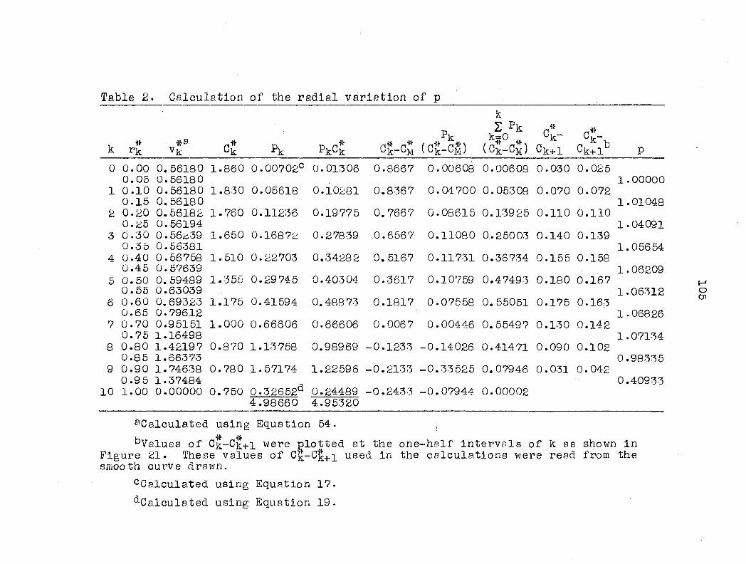
Table 2. Calculation of the radial variation of p

k

k

CD * M > Pk PkCk C 1# k-^M

A k=0 Ck ' (Ck-Cn) c^+i <&> p

0 0.00 0.05

0. 0. 56180 56180

1 .860 0 .00702° 0 .01306 0. 8667 0 .00608 0.00608 0.030 0.025 1 .00000

1 0.10 0.15

0. 0. 56180 56180

1 .830 0 .05618 0 .10281 0. 8367 0 .04700 0.05308 0.070 0.072 1 .01048

2 0.20 0.25

0. 0. 56182 56194

1 .760 0 .11236 0 .19775 0. 7667 0 .08615 0.13925 0.110 0.110 1 .04091

3 0.30 0.35

0. 0. 56239 56381

1 .650 0 .1687% 0 .27839 0. 6567 0 .11080 0.25003 0.140 0.139 1 .05654

4 0.40 0.45

0. 0. 56758 57639

1 .510 0 .22703 0 .34282 0. 5167 0 .11731 0.36734 0.155 0.158 1 .06209

5 0.50 0.55

0. 0.

59489 63039

1 .355 0 .29 745 0 .40304 0. 3617 0 .10759 0.47493 0.180 0.167 1 .06312

6 0.60 0.65

0. 0. 69323 79612

1 .175 0 .41594 0, .48873 0. 1817 0 .07558 0.55051 0.175 0.163 1 .06826

7 0.70 0.75

0. 1. 95151 16498

1 .000 0 .66606 0 .66606 0. 0067 0 .00446 0.55497 0.130 0.142 1 .07134

8 0.80 0.85

1. 1. 4219 7 66373

0 .870 1 .13758 0, .98969 -0. 1233 -0 .14026 0.414 71 0.090 0.102 0 .98335

9 0.90 1. 74638 0 .780 1 .57174 1 .22596 -0. 2133 -0 .33525 0.07946 0.031 0.042 0.95 1. 37484

.32652d 0 .40933

10 1.00 0. 00000 0 .750 0 .32652d 0 .24489 -0. 2433 -0 .07944 0.00002 4.98660 4.95320

^Calculated using Equation 54. j

^Values of C^-C^+l were plotted at the one-half intervals of k as shown in Figure 21. These values of G^-C^+]_ used in the calculations were read from the smooth curve drawn.

^Calculated using Equation 17.

^Calculated using Equation 19.

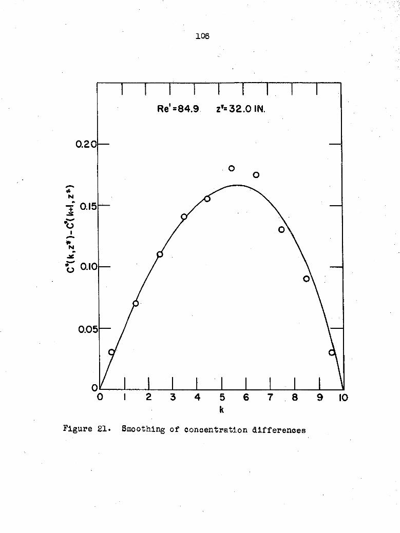
106

Re'=84.9 z*= 32.0 IN.

0.20

0.15

0.10

0.05

0 2 3 4 5 6 7 8 9 1 0 k

Figure 21. Smoothing of concentration differences

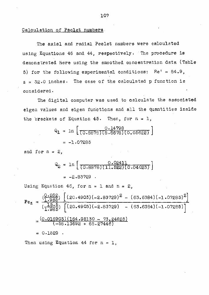
107

Calculation of Peclet numbers

The axial and radial Peclet numbers were calculated

using Equations 46 and 44, respectively. The procedure is

demonstrated here using the smoothed concentration data (Table

5) for the following experimental conditions: Re1 = 84.9,

z = 32«0 inches. The case of the calculated p function is

considered.

The digital computer was used to calculate the associated

eigen values and eigen functions and all the quantities inside

the brackets of Equation 45. Then, for n = 1,

fl ^ T 0.14798 1 *1 = ln L(0.8878)(8.6678)(0.05622) J

= -1.07285

and for n = 2,

0 = 1n I" 0.02411 1 2 1 [ (0.8878)(11.522)(0.04023) J

= -2.83729 .

Using Equation 46, for n = 1 and n = 2,

[(20.4903) (-2.83729)2 - ( 63.6384) (-1.07285)2]

(irfef) [(20*4903)(-2.83729) - (63.6384)(-1.07285)1 Pe7. =

_ (0.016903) (164.95130 - 73.24825) ~ (-58.13692 + 68.27446)

= 0.1529 •

Then using Equation 44 for n = 1,

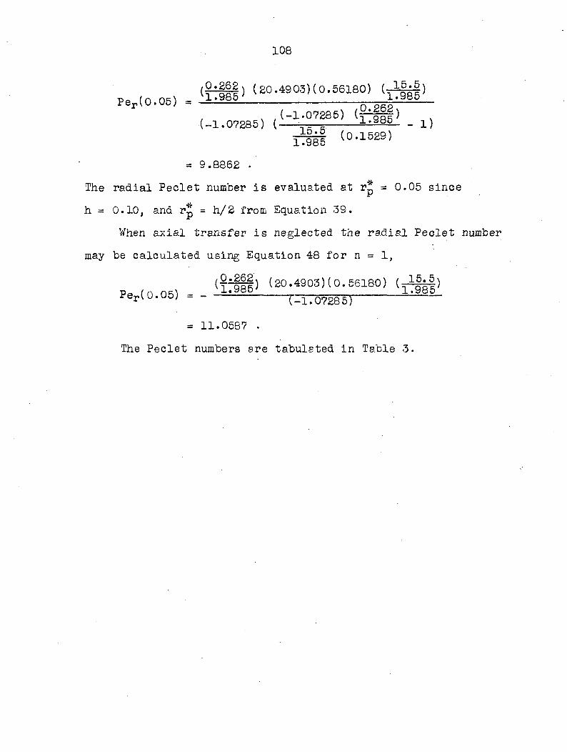
108

(^HI) (20.4903)(0.56180) (-%g) Per(0.05) = -isse 1-985

(-1.07285) (t'1:°7fS) (l-985' - 1)

Ï7§g§ (0-1529)

= 9.8862 •

The radial Peclet number is evaluated at r* = 0.05 since

h = 0.10, and rp = h/2 from Equation 39.

When axial transfer is neglected the radial Peclet number

may be calculated using Equation 48 for n = 1,

(t4SI) (20.4903) (0.56180) (^%#) Per(0.06) - - t-x.07285)

= 11.0587 .

The Peclet numbers are tabulated in Table 3.

109

Tabular Results

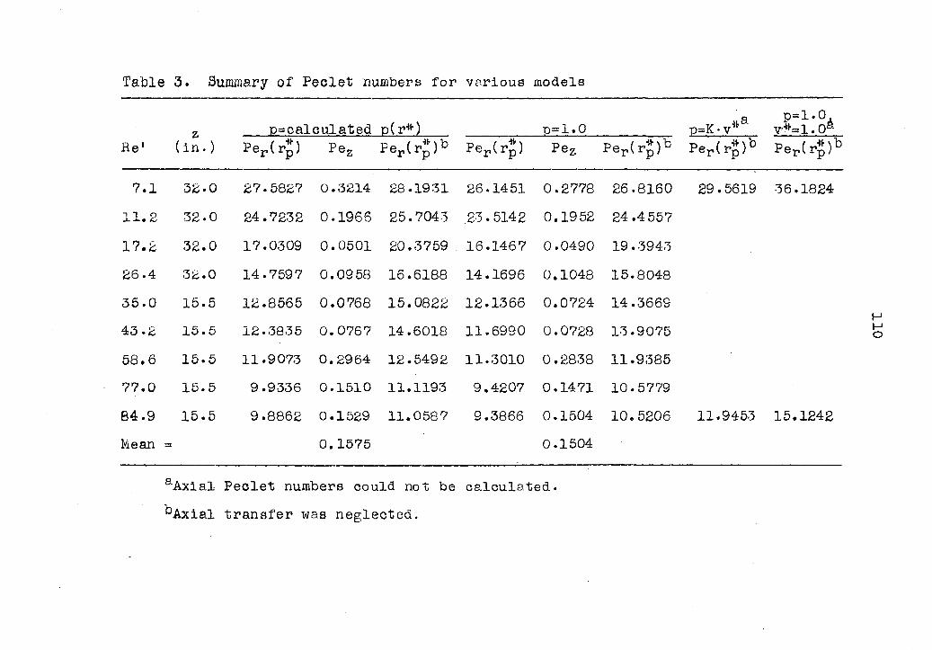
Table 3. Summary of Peclet numbers for various models

Z, p=calculated p(r*)

o

i—( ii P p=K- v4*a

p=1.0 v*=1.0&

Re' (in. ) Per(rp) Fez Per(rJ)b Per(rp) Pez Per(r»)b Per(rp)b Per(rp)^

7.1 32. 0 27.5827 0.3214 28.1931 26.1451 0.2778 26.8160 29.5619 36.1824

11.2 32. 0 24.7232 0.1966 25.7043 23.5142 0.1952 24.4 557

17.2 32. 0 17.0309 0.0501 20.3759 16.1467 0.0490 19.3943

26.4 32. 0 14.7597 0.0958 16.6188 14.1696 0.1048 15.8048

35.0 15. 5 12.8565 0.0768 15.0822 12.1366 0.0724 14.3669

43 .2 15. 5 12.3835 0.0767 14.6018 11.6990 0.0728 13.9075

58.6 15. 5 11.9073 0.2964 12.5492 11.3010 0.2838 11.9385

77.0 15. 5 9.9336 0.1510 11.1193 9.4207 0.1471 10.5779

84.9 15. 5 9.8862 0.1529 11.0587 9.3866 0.1504 10.5206 11.9453 15.1242

Mean 0.1575 0.1504

^Axial Peclet numbers could not be calculated,

bAxial transfer was neglected.

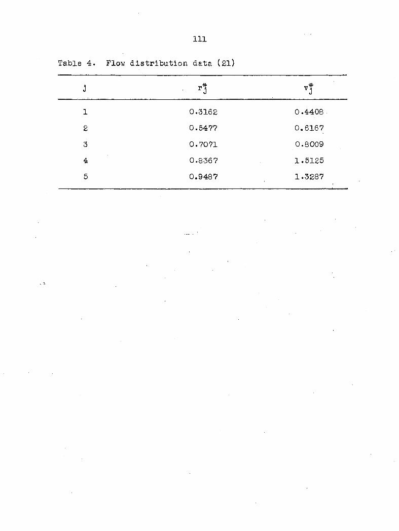
Ill

Table 4. Flow distribution data (21)

J • 'Î '?

1 0.3162 0.4408

2 0.5477 0.6167

3 0.7071 0.8009

4 0.8367 1.5125

5 0.9487 1.3287

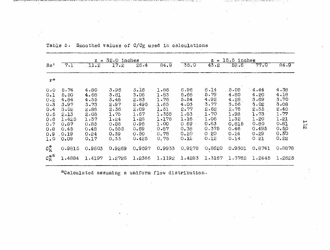
Table 5• Smoothed values of G/Ce used In calculations

z - 32.0 inches z = 15.5 inches Re1 7.1 11.2 17.2 26.4 84.9 35.0 43.2 58.6 77.0 84.9

0.0 5.74 4.80 0.1 5.50 4.68 0.2 4.84 4.3 5 0.3 3.97 3 .73 0.4 3.02 2.86 0.5 2.13 2.05 0.6 1.425 1.37 0.7 0.87 0.85 0.8 0.45 0.48 0.9 .0.19 0.24 1.0 0.09 0.17

CM

CM*

0.9815

1.4884

0.9603

1.4197

3.96 3.16 1.86 6.96 3.81 3.06 1.83 6.66 3.46 2.83 1.76 5.54 2.97 2.495 1.65 4.03 2.36 2.09 1.51 2.77 1.75 1.67 1.355 1.83 1.24 1.28 1.175 1.16 0.85 0.96 1.00 0 6 9 0.555 0.69 0.87 0.38 0.39 0.50 0.78 0.20 0.33 0.425 0.75 0.12

0.9269 0.9597 0.9933 0.9278

1.2726 1.2366 1.1192 1.4283

6.14 5.79 4.92 3.77 2.62 1.70 1.06 0.63 0.375 0 20 0.12

0.8620

1.3167

5.05 4 .44 4.38 4.80 4 .20 4.18 4.28 3 .69 3.70 3.56 3 .02 3.08 2.75 2 .35 2.40 1.98 1 .73 1.77 1.32 1 .20 1.21 0.815 0 .80 0.81 0.46 0 .495 0.5,0 0.24 0 .29 0.3b 0.14 0 21 0.22

0.9301

1.3762

0.8741

1.2445

0.8878

1.2625

^-Calculated assuming a uniform flow distribution.

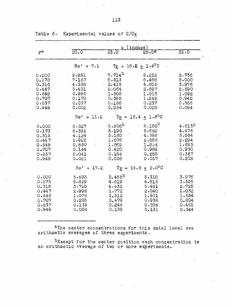
113

Table 6. Experimental values of C/Cg

z (inches) r* 20.0 23.0 26.0^ 32.0

Re' = 7.1 Tg = 16.2 £ 1.4°C

0.000 . 9.981 7.714% 8.252 5.736 0.173 7.157 6.513 6.468 5.000 0.316 4.338 5.415 4.605 3.976 0.447 3.431 2.064 2.697 2-590 0.548 0.990 1.505 1.513 1.692 0.707 0.179 0.585 1.242 0.942 0.837 0.037 0.156 0.237 0.366 0.949 0.002 0.034 0.029 0.094

ii CD

11.2 TE = = 15.4 + 1.6°C

0.000 8.527 6.506% 6.168^ 4.813% 0.173 6.392 5.190 5.652 4.475 0.316 4.124 5.160 4.386 3.664 0 .44 7 2.925 1.576 2.866 2.294 0.548 0.850 1.562 1.824 1.695 0.707 0.144 0.420 0.989 0.930 0.837 0.041 0.184 0.288 0.367 0.949 0.021 0.058 0.057 0.218

0.000 0.173 0.316 0.447 0.548 0.707 0.837 0.949

Re1 = 17.2

6.493 5.829 3.720 2.998 1.075 0.296 0.135 0.054

te =

5.485% 4.619 4.432 1.772 1.512 0.479 0.244 0.139

6 + 2.0°C

5.318 4.815 3.481 2.840 1.901 0.938 0.504 0.131

3.976 3 .558 2.725 2.032 1.554 0.804 0.482 0.344

aThe center concentrations for this axial level are arithmetic averages of three experiments.

%Except for the center position each concentration is an arithmetic average of two or more experiments.

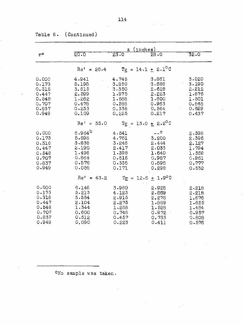
114

Table 6. (Continued)

z (inches) r* 20.0 23.0 26.0 32.0

S)

CD 11 26 .4 TE = 14 .1 + 2.1 C

0.000 4.941 4.745 3.861 3.020 0.173 5.198 3.850 3.688 3.190 0.316 3. 515 3.350 2.625 2.212 0.447 2.599 1.975 2.223 1.876 0.548 1.262 1.588 1.600 1.501 0. 707 0.478 0.588 0.963 0.848 0.837 0.233 0.338 0.564 0.629 0.949 0.109 0.225 0.217 0.437

Re' = 35 .0 tE = 13 .0 + 2.2°C

0.000 6.964% 4.541 c 2.598 0.173 5.898 4.751 3.200 2.396 0.316 3.838 3.246 2.444 2.127 0.447 2.190 2.417 2-033 1.794 0.548 1.496 1.398 1.640 1.558 0.707 0.664 0.616 0.987 0.961 0.837 0.576 0.336 0.696 0.777 0.949 0.058 0.171 0.298 0.532

Re' = 43 .2 TE = 12 .6 + 1.9°C

0.000 6.146 3.960 2.928 2.218 0.173 5.213 4.123 2.889 2.218 0.316 3.554 2.915 2.278 1.876 0.447 2.104 2.275 1.889 1.655 0.548 1.344 1.268 1.528 1.464 0.707 0.600 0.746 0.972 0.957 0.837 0.512 0.457 0.733 0.808 0.949 0.090 0.223 0.411 0.576

cNo sample was taken.

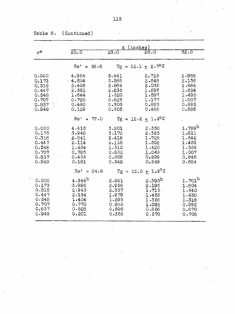
115

Table 6. (Continued)

z (inches) r* 20.0 23.0 26.0 32.0

Re' = 58 .6 te = 12. 1 + 2.7°C

0.000 4.954 3.441 2.716 1.968 0.173 • 4.654 3.566 2.648 2.136 0.316 3.406 2.664 2.035 1.864 0.447 2.391 2.235 1.696 1.654 0.548 1.644 1.320 1.597 1.495 0.707 0.728 0.826 1.177 1.007 0.837 ' 0.480 0.603 0.893 0.895 0.949 0.129 0.305 0.488 0.686

Re' = 77 .0 TE = 12. 2

o

o 1—

1 +!

0.000 4.416 3.201 2.530 1.789% 0.173 3.948 3.172 2.325 1.811 0.316 2.841 2.419 1.728 1.642 0.447 2.114 2.118 1.502 1.459 0.548 1.454 1.312 1.420 1.354 0.707 0.783 0.832 1.049 1.007 0.837 0.434 0.606 0.899 0.846 0.949 0.181 0.342 0.549 0.684

Re' = 84 .9 TE = 12. ,0 + 1.9°C

0.000 4,344% 2.981 2.393% 1.701% 0.173 •3.996 2.958 2.193 1.804 0.316 2.943 2.337 1.715 1.640 0.447 2-134 1.9 79 1.455 1.430 0.548 1.454 1.295 1.356 1.318 0.707 0.770 0.888 1.092 0.992 0.837 0.528 0.596 0.856 0.870 0.949 0.201 0.368 0.570 0.706

116

APPENDIX B

The numerical solution of the Sturm-Liouville problem

and some of the associated calculations with the experimental.

concentration data were performed by an IBM 7074 digital com­

puter . The computer program was written in the FULL FORTRAN

IBM language and was essentially a combination of three sep­

arate programs: the major program, the subroutine for cal­

culating the eigen values (SUBROUTINE EIG-N), and the sub­

routine for calculating the eigen functions (SUBROUTINE VCTR).

The major variables used in the program in the order of their

first appearance in the FORTRAN statements are defined as

follows:

IDATA a control integer defining the amount of input and giving a dump of the core memory if desired

a control integer specifying the form ( equation or tabulai?) of the input flow distribution

a control integer specifying the form (equation or tabular) of the input p function

constant in the flow distribution equation, A

constant in the flow distribution equation, B

constant in the flow distribution equation, generally zero

exponent in the flow distribution equation, n

exponent in the flow distribution equation, m

constant in the p function equation; used only in the case 3 radial diffusivity model

constant in the p function equation; used only in the case 3 radial diffusivity model

JDATA

KDATA

VI

V2

V3

NX

M

F

G

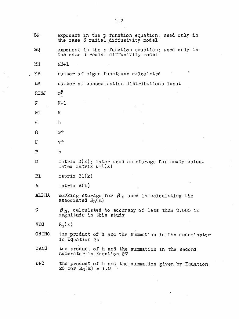
117

SP exponent in the p function equation; used only in the case 3 radial diffusivity model

SQ, exponent in the p function equation; used only in the ease 3 radial diffusivity model

NN 2N+1

KP number of eigen functions calculated

LV number of concentration distributions input

RINJ r I

N M+l

NI N

H h

R r*

U v*

P p

D matrix D(k); later used as storage for newly calcu­lated matrix D-l(k)

B1 matrix Bl(k)

A matrix A(k)

ALPHA working storage for /? n used in calculating the associated Rn(k)

G j3 n, calculated to accuracy of less than 0.005 in magnitude in this study

VEC Rn(k)

OR'THO the product of h and the summation in the denominator in Equation 25

CANS the product of h and the summation in the second numerator-in Equation 27

DNC the product of h and the summation given by Equation 26 for R0(k) = 1.0

118

ANC the product of h and the summation given by Equation 26 for any Rn(k)

CC calculated concentrations, used only in checking to determine which concentration distributions could be used to calculate p

WL large increment used in approximating /3 n; in this study WL = 0.5

WF small increment used in approximating )S n; in this study WF = 0.005

KEV number of eigen values calculated

PI working storage for evaluating the determinant of (A(k) - @1) for a previously estimated Bn

G-Alvi estimated j3 n

SEC previously estimated jSn

POL working storage for evaluating the determinant of (A(k) - /3l) for an estimated & n

FT storage for any estimated /3n

SAM improved estimate of /3n using small increment WL

V temporary storage for a given Rn(k)

The FORTRAN statements are listed in sequence in Figure

22.

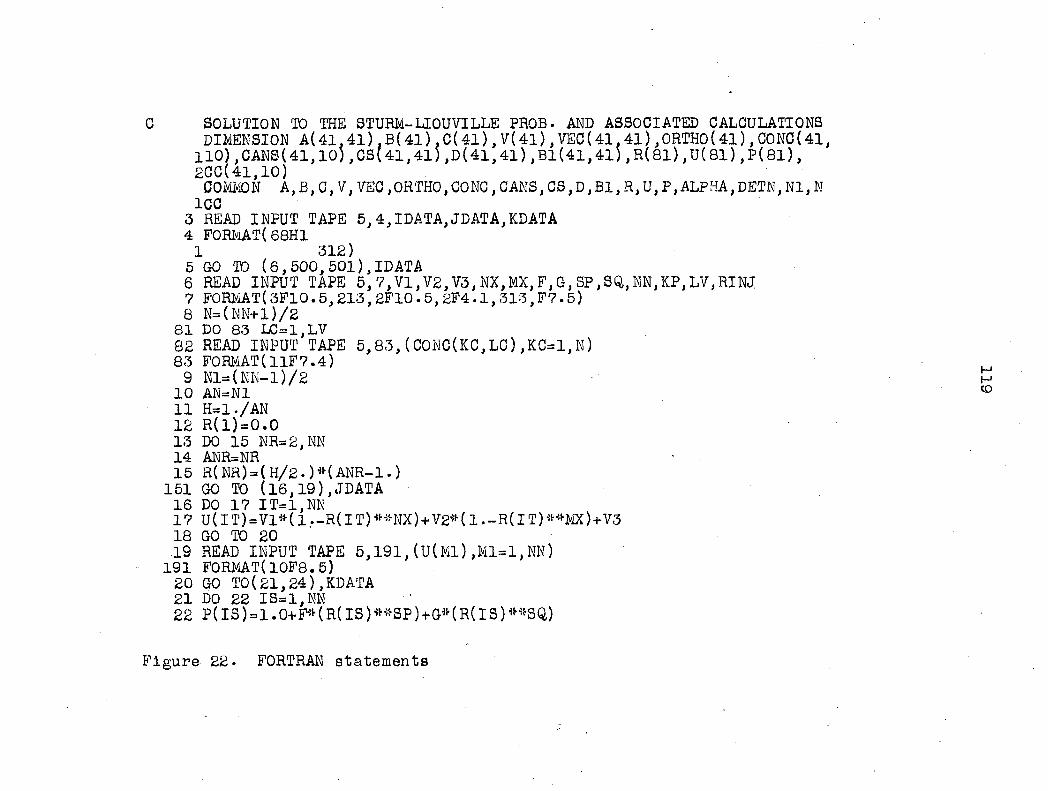
C SOLUTION TO THE STURM-LIOUVILLE PROS. AND ASSOCIATED CALCULATIONS DIMENSION A(41,4l),B(4l).C(4l),V(4l),VEC(41,4l),0RTH0(4l),C0NC(41,

ll0),CANS(41,10),CS(41,4l),D(41,4l),Bl(4l,41),R(8l),U(8l),P(8l), 200(41,10) COMMON A,B,C,V,VEC,ORTHO,CONO,CANS,CS,D,B1,R,U,P,ALPHA,DETN,NI,N

ICC 3 READ INPUT TAPE 5,4, IDA TA, JDATA, KDATA. 4 FORMAT( 68H1 1 312) 5 GO TO ( 6 , 500, 501 ), IDATA 6 READ INPUT TAPE 5, 7,VI,V2,V3,NX,MX, F, C-, SP,SQ, NN,KP,LV,RINJ 7 FORMAT( 3F10.5, 213, 2F10. 5, 2F4.1,31-3, F7.5) 8 N=(NN+l)/2 81 DO 83 LC=1,LV 82 READ INPUT TAPE 5,83,(CONC(KC,LC),KC=1,N) 83 FORMAT(11F 7.4) 9 Nl=(NN-l)/2 10 AN=N1 11 H=1./AN 12 R(1)=0.0 13 DO 15 NR=2,NN 14 ANR=NR 15 R(NR)=(H/2.)*(ANR-1.)

151 GO TO (16,19),JDATA 16 DO 17 IT=1,NN 17 U(IT) = V1*(1.-R(IT)"*NX) + V2*(l.-R(IT)**MX)+V3 18 GO TO 20 19 READ INPUT TAPE 5,191,(U(Ml),M1=1,NN)

191 F0RMAT(10F8.5) 20 GO TO(21,24),KDATA 21 DO 22 IS=1,NN 22 P(IS)=1.0+F*(R(IS)**SP)+G*(R(IS)**SQ)

Figure 22. FORTRAN statements

23 GO TO 26 24 READ INPUT TAPE 5, 25, ( P( ISS ), ISS=1, NN) 25 FORMAT(10F8.5) 26 DO 29 IR=1,N 27 DO 28 IC=1,N 28 D(IR,IC)=0.0 29 CONTINUE 30 D(1,1)=H*H*0.25*U(2)"R(2) 31 D(N,N)=H*H*0.25*U(NN-1)#R(NN-1 ) 32 KN=N-1 33 DO 35 IA=2,KN 34 L=2*IA-1 35 D(IA,IA)=H*H*U(L)*R(L) 36 DO 39 IBR=1,N 37 DO 38 IBC=1,N 38 Bl(IBR,IBG)=0.0 39 CONTINUE 40 Bl(l,l)=P(2)*R(2) 41 B1(1,2)=-P(2)*R(2) 43 DO 47 KR=2,KN 44 Ll= 2"KR-2 45 Bl(KR,KR)=P(Ll)*R(Ll)+P(Ll+2)»R(Ll+2) 46 Bl(KR,KR-l)=-P(Ll)*R(Ll) 4 7 B1 ( KR, KR+1 ) = -P ( L1+ 2 ) *R( L1+ 2 ) 48 Bl( N,N-l)=-P(NN-l)#R(NN-l) 49 B1 ( N,N)=P(NN-1)*R(NN-1)

DO 75 1=1,N 75 D(I,I)=1./D(I,I)

DO 76 1=1,N DO 76 J=1,N

76 A(I,J)=0. A(1,1)=D(1,1)*B1(1,1) A(N,N)=D(N,N)*B1(N,N)

Figure 22. (Continued)

DO 80 1=2,KM K1=I-1 K2=I+1 DO 80 KI=K1,K§

80 A(I,Kl)=D(I,I)*Bl(I,KI) ' • A(1,2)=D(1,1)*B1(1,2) A(N,N-1)=D(N,N)»B1(N,N-1) NI=1 DETK=100000.0 CALL EIGN

DO 120 1=1,KP ALPHA=C(I) CALL VCTR

DO 110 IJ=1,N 110 VEC( IJ ,l) = v(lj)/v(l) 120 CONTINUE 90 DO 91 1=1,N 91 B(I)=0.0

1203 KF=N-2 1204 DO 1215 IB=1,KP 1201 AN0=0.0 1205 DO 1207 IB0=2,KN 1206 JB0=2*IB0-1 1207 AN0=AN0+VEC(IBO,IB)*VEC(IBO,IB)*R(JBO)*U(JBO) 1208 0RTH0(IB)=H*(AN0+0.25*U(2)*R(2)*VEC(1,IB)*VEC(1,IB)+0.25*U(NN-1)

1R(NN-1)*VEC(N,IB)*VEC(N,IB)) 1209 DO 1214 IBA=1,LV 1202 ANS=0.0 1210 DO 1212 IBB=2,KN 1211 IRB=2*IBB-1 1212 ANS=ANS+C0NC(IBB,IBA)#R(IRB)»U(IRB)*VEC(IBB,IB)

Figure 22. (Continued)

1213 CANS(lB,IBA)=H*(ANS+0.25*U(2)*R(2)*VEC(l,IB)*CONC(l,IBA)+0.25* 1U(NN-1)*R(NN-1)#VEC(N,IB)*C0NC(N,IBA))

1214 CONTINUE 1215 CONTINUE

DNC=H*(0.25*R(2)*U(2)+RINJ*U(3)) DO 95 NC=1,KP ANC=H*(0.25*R(2) *U( 2)*VEC ( 1,NC)+RINJ#U(3)»VEC(2,NC))

95 B(NC)=ORTHO(l)*ANC/(ORTHO(NC)#DNC) 1216 DO 1222 LV1=1,LV 1217 DO 1221 NC=1,N 1218 01=0.0 1219 DO 1220 KP1=1,KP 1220 CI = CI + VEClNC,KPl)*CANS(KPl,LVl)/ORTHO(KPl) 1221 CC(NC,LVl)=CI 1222 CONTINUE 121 WRITE OUTPUT TAPE 10,4,IDATA,JDATA,KDATA 122 WRITE OUTPUT TAPE 10,123 123 FORMAT(37HJ J EIGEN VALUE(j) A(j) ) 124 DO 126 J0=1,KP 125 FORMAT(1H 14,2E18.8) •126 WRITE OUTPUT TAPE 10,125,JO,C(Jo),B(JO) 127 DO 134 JV=1,KP,5 128 JC=JV+4 129 WRITE OUTPUT TAPE 10 130 130 FORMAT(114HJ I R(I) .RVEL(I) PE(l) EIGEN FUNCT(I.l) E

1 F(I,2) E F( 1,3) E F( 1,4) E F(I,5) ) 131 DO 132 IW=1,NN 1310 IV=(IW+l)/2 132 WRITE OUTPUT TAPE 10,133, IW, R( IW),U( IW), P( IW), ( VEC( IV, JT) , JT=JV, JC

133^F0RMAT(1H 13,3F9.5,5E17.8) 134 CONTINUE 140 DO 147 KJ=1, LV, 5 141 KF=KJ+4

Figure 22. (Continued)

142 WRITE OUTPUT TAPE 10,143 143 FORMAT(103H1 J ORTHO(j) CANS(J l) CANS(J,2)

1 CANS(J,3) CAKS(J,4) CAKS(J,5) ) 144 DO 146 JN=1,KP 145 WRITE OUTPUT TAPE 10,146,JN,ORTHO(JN),(CANS(JN,Jl),JI=KJ,KF) 146 FORMAT(1H I3,E16.8,5E17.8) 14? CONTINUE 148 DO 1542 LV2=1,LV, 5 149 LY3=LV2+4 150 WRITE OUTPUT TAPE 10,1501 1501 FORMAT(113H1 I R(I) CONC(l,l) CC(I,l) C0NC(l,2) CC(I,2)

1C0NC(I,3) GC(1,3) C0NC(I,4) CC(l,4) CONG(I,5) CC(I,5) ) 152 DO 1541 N9=1,N 153 N8=2*N9-1 154 WRITE OUTPUT TAPE 10,1541,N9,R(N8),(CONC(N9,LV4),CC(N9, LV4), LV4=

1LV2,LV3) 1541 FORMAT(1H I3,F9.5,F9.4,9F10.4) 1542 CONTINUE 499 GO TO 3 500 STOP 89 501 STOP 502 END

SUBROUTINE EIGN 601 DIMENSION A(41,4l).B(4l),C(4l),V(4l),VEC(4l,4l),0RTH0(4l),C0NC(41,

110),CANS(41,10),GS(41,41),D(41,41),81(41,41),R(81),U(8l),P(8l), 200(41,10)

602 COMMON A,B,G,V,VEC,ORTHO,CONG,CANS,GS,D,Bl,R,U,P,ALPHA,DETN,NI,N, ICC

603 READ INPUT TAPE 5,604,WL,WF,KEV 604 FORMAT(2E16.8,18) 605 Pl=-0.00000001 606 FA=-WL

Figure 22. (Continued)

628 DO 699 1=1,KEV 6,30 DO 657 J* 1,999

SJ=J GAk=FA+SJ»WL SEC=GAM B(l)=A(1,l)-GAM B(2)=(A(2,2)-0AM)*B(l)-A(l,2)*A(2,l)

650 DO 651 K=3,N 651 B(K)=(A(K,K)-GA%)*B(K-l)-A(K-l,K)*A(K,K_l)*B(K-2) 652 POL=B(N) 653 IF(POL)655,671,654 654 IF(Pl)658,656,656 655 IF(P1)666,656,658 656 P1=B(N)

6561 FT=GAM 657 CONTINUE 658 DO 670 L=l,999

5AM=FT+WF SEC=SAM

660 B( l)=sA( 1, l)-SAM 661 B(2)=(A(2,2)-SAM)*B(l)-A(l,2)*A(2,l) 662 DO 663 KF=3,N 663 B(KF)=(A(KF,KF)-SAM)*B(KF-l)-A(KF-l,KF)*A(KF,KF-l)*B(KF-2) 664 POL=B(N) 665 I1T( POL) 667, 681,666 666 IF(Pi)690,669,669 667 IF(Pi)669,669,690 669 FT=SAM 670 P1=B(N) 671 C ( I )=GAM 672 FA=GAM 673 P1=B(N)

GO TO 699 681 C(I)=SAM

Figure 22. (Continued)

682 FA=SAM 683 P1=B(N)

GO TO 699 690 C(I )=FT-ABSF(Pl) ""•( FT-SEC )/(ABSF(P1)+ABSF(POL) ) 692 FA=FT 693 P1=P0L 699 CONTINUE

RETURN END

SUBROUTINE VGTR DIMENSION A(41,41),B(41),C(41),V(41),VEC(41,41),0RTH0(4l),C0NC(41

110) , CANS ( 41,10),CS(41,41; ,D ( 41,41) ,Bl(41,41 ) ,R( 81), U( 81)', P( 81 ), 2CG(41,10) COMMON A,B,C,V,VEC,ORTHO,GONG,CANS,CS,D,B1,R,U,P,ALPHA,DETN,NI,N

ICC 513 V(l)=1.0 514 V(2)=-1.*(A(1,1)-ALPHA)*V(1)/A(1,2) 515 DO 516 JV=3,N 516 V(JV)=-l.*(A(jV_l,JV-2)"V(JV-2)+(A(jV-l,JV-l)-ALPHA)*V(jV_l))/

1A(JV-1,JV) RETURN END

Figure 22. (Continued)