Liquefaction Assessment through Machine Learning

Approach

S. García, Instituto de Ingeniería, Universidad Nacional Autónoma de México, México

E. Ovando-Shelley Instituto de Ingeniería, Universidad Nacional Autónoma de México, México

J. Gutiérrez & J. García Escuela Superior de Ingeniería y Arquitectura, Instituto Politécnico Nacional, México

SUMMARY:

This paper presents a machine learning scheme for assessing the liquefaction potential of soils based on

geotechnical, geometrical and seismic load parameters. A relatively large database consisting of CPT and Vs

measurements and field liquefaction performance observations of historical earthquakes is analyzed. This

database is used to construct a nonlinear environment where the occurrence and nonoccurrence of liquefaction

can be predicted using neural networks and classification trees. The successfully trained and tested scheme is

composed of i) a neural network to map automatically some soil properties and seismic loading values to the

liquefaction occurrence and ii) a classification tree that explain the liquefaction occurrence through a

multidimensional if-then approach. The data points, measured and estimated, collectively define the liquefaction

boundary surface, the limit state nonlinear-function. Based on these newly developed models, intelligent

analyses of the cases in the database are conducted using simple mapping lines. The Machine Learning models,

no necessarily expressed as functions, provide a simple means for knowledge-based evaluation of the

liquefaction potential that compare favorably to a widely used existing methods.

Keywords: liquefaction potential, cyclic resistance ratio, cyclic shear stresses, neural networks, regression trees

1. INTRODUCTION

Over the past forty years, scientists have conducted extensive research and have proposed many

methods to predict the occurrence of liquefaction; one of the most destructive phenomena caused by

earthquakes. In the beginning, undrained cyclic loading laboratory tests had been used to evaluate the

liquefaction potential of a soil (Castro et al., 1982) but due to difficulties in obtaining undisturbed

samples of loose sandy soils, many researchers have preferred to use in situ tests (Seed et al., 1983). In

a semi-empirical approach the theoretical considerations and experimental findings provides the

ability to make sense out of the field observations, tying them together, and thereby having more

confidence in the validity of the approach as it is used to interpolate or extrapolate to areas with

insufficient field data to constrain a purely empirical solution. Empirical field-based procedures for

determining liquefaction potential have two critical constituents: i) the analytical framework to

organize past experiences, and ii) an appropriate in situ index to represent soil liquefaction

characteristics. The original simplified procedure (Seed and Idriss, 1971) for estimating earthquake-

induced cyclic shear stresses continues to be an essential component of the analysis framework. The

refinements to the various elements of this context include improvements in the in-situ index tests

(e.g., standard penetration test SPT, cone penetration test CPT, self-boring pressure meter tests BPT,

shear wave velocities Vs), and a better, more organized compilation of liquefaction/no-liquefaction

cases.

The objective of the present study is to produce an empirical machine learning ML method for

evaluating liquefaction potential. ML, a branch of cognitive computation, is a scientific discipline

concerned with the design and development of algorithms that allow computers to evolve behaviours

based on empirical data, such as from sensor data or databases. Data can be seen as examples that

illustrate relations between observed variables. A major focus of ML research is to automatically learn

to recognize complex patterns and make intelligent decisions based on data; the difficulty lies in the

fact that the set of all possible behaviours given all possible inputs is too large to be covered by the set

of observed examples (training data). Hence the learner must generalize from the given examples, so

as to be able to produce a useful output in new cases. In the following two ML tools, Neural Networks

NNs and Classification Trees CTs, are used to evaluate liquefaction potential and to find out the

liquefaction control parameters, including earthquake and soil conditions. For each of these

parameters, the emphasis has been on developing relations that capture the essential physics while

being as simplified as possible. The proposed cognitive environment permits an improved definition of

i) seismic loading or cyclic stress ratio CSR, and ii) the resistance of the soil to triggering of

liquefaction or cyclic resistance ratio CRR.

2. MACHINE LEARNING: NEURAL NETWORKS AND REGRESSION TREES

The aim of machine learning ML users is to comprehend the structures that are abstracted from a

dataset; however, the emphasis in ML research literature tends to focus very much on prediction

ability. Several different representations have been developed in ML having different degrees of

expressive power—and therefore comprehensibility. In this investigation the extremes will be

implemented: a “black-box” (neural networks) model and a “transparent-box” (regression trees)

model.

Neural Networks NN are computational tools whose intention is to mimic the biological

characteristics of the human learning. Like biological neurons, they consist of interconnected

information processing neural elements (neurons) working in union to make decisions, classifications,

and predictions. NN are capable of learning linear and nonlinear functions that make them leading

machinery in the analysis of complex relations expressed through data. Interconnections among

neurons are established by weights, which are applied to all values passing through one neuron to

another. Changing weights improves adaptabilities and prediction capabilities of these devices. NN are

arranged mainly in three layers namely: input layer; output layer, and the hidden layers. Through the

learning process, input and output data of a specific problem are given, and the aforementioned

weights among neurons are updated without requiring human development of algorithms. In the

validation phase, the trained network makes predictions for a new set of data that has never been

introduced during the previous phases. The neural network will provide accurate prediction, as long as

large volumes of data covering all possible governing parameters and field conditions are used during

the learning process. Extensive information regarding the characteristics of neural network

methodology is outlined in detail in the literature (Ghaboussi, 1992; Hammerstrom, 1993; Flood and

Kartam, 1994).

However, research on learning is made up of diverse subfields; at one extreme there are adaptive

systems that monitor their own performance and attempt to improve it by adjusting internal parameters

(e.g. Samuel, 1967; Michie, 1982; Quinlan, 1969) and a quite different approach sees learning as the

acquisition of structured knowledge in the form of concepts (Hunt, 1962; Winston, 1975),

discrimination nets (Feigenbaum and Simon, 1963), or production rules (Buchanan,1978). I this

branch a crucial concern is the representation in a more direct way to understand the knowledge

structures and relate them to the data from they came. The basic representations are trees, rule sets,

and graphs. Within each are many variants that can be traced that proceeds from simple structures to

ones with higher degrees of semantic expressiveness. In general, one would expect an expressive

language to permit more compact representations of complex decisions, but impose greater demands

on the user’s ability and motivation to learn how to interpret the result; it is a modeler mission to get

the balance between demands and benefits for particular analysis models.

Decision trees, either classification or regression trees, are especially attractive type of models for

three main reasons: i) intuitive representation, the resulting model is easy to understand and assimilate

by humans (Breiman et al., 1984), ii) nonparametric models, no intervention being required from the

user, and thus they are very suited for exploratory knowledge discovery, iii) scalable algorithms,

performance degrades gracefully with the increase of the size of training data (Gehrke et al., 1998;

Murthy, 1995; Lim et al., 1997). For evaluating learning performance (how successfully a model

learns a concept) exist descriptive (captures the training data), predictive (generalizes to unseen data)

and explanatory (provides a plausible description of the concept to be learned) levels. In general, a

model is ranked as successful if, given instances labeled with some distinguished attributes (target),

the modeling goal is acquired (predict target for new unlabeled instances and reveal understand

structure underlying data). A “divide-and-conquer” approach to the problem of learning from a set of

independent, contaminated, uncertain and poor understood instances leads naturally to the style of

representation called a tree. In this investigation classification trees CTs are used to generate learning

about the seismic attenuation phenomena. CTs are decision trees for class assignation problems. A

class label is associated to every node with a functional dependency of some of the inputs presented.

For the interested reader about the CTs characteristics see Garcia & Romo (2006).

3. BASIC FRAMEWORK FOR SEMI-EMPIRICAL PROCEDURES FOR LIQUEFACTION

ASSESMENT

The factor of safety FS against the initiation of liquefaction of a soil under a given seismic loading is

commonly described as the ratio of cyclic resistance ratio (CRR), which is a measure of liquefaction

resistance, over cyclic stress ratio (CSR), which is a representation of seismic loading that causes

liquefaction, symbolically FS=CRR/CSR. The reader is referred to Seed and Idriss (1971), Youd et al.

(2001), and Idriss and Boulanger (2004) for a historical perspective of this approach. The term CSR

( ) (3.1)

is function of the vertical total stress of the soil at the depth considered, the vertical effective stress

, the peak horizontal ground surface acceleration , a depth-dependent shear stress reduction

factor (dimensionless), a magnitude scaling factor (dimensionless). For CRR, different in situ-

resistance measurements and overburden correction factors are included in its determination; both

terms operate depending of the geotechnical conditions. Details about this definitions in Idriss and

Boulanger,(2004) and Youd et al. (2001).

In CSR determination is important to include a stress reduction coefficient for taking into account the

flexibility of the soil column (e.g., corresponds to rigid body behavior). The factor 0.65 is used

to convert the peak cyclic shear stress ratio to a cyclic stress ratio that is representative of the most

significant cycles over the full duration of loading. The values of CSR calculated using equation (3.1)

pertain to the equivalent uniform shear stress induced by an earthquake of magnitude (moment

magnitude). It is also necessary to adjust these values so that they would pertain to ground motions

generated by an earthquake having a . On the other hand, for CRR, the purpose of the

overburden normalization is to obtain quantities that are independent of , and thus more uniquely

relate to the sand's relative density.

The correlation of the CSR (required to cause liquefaction) to in situ resistance is thus directly affected

by the choice of the correction expression, as has been illustrated for many researchers (Idriss and

Boulanger, 2004).The correction factors have been included in the conventional analytical frameworks

to organize and to interpret the historical data. The correction factors try to improve the consistency

between the geotechnical/seismological parameters and the observed liquefaction behavior, but they

are a consequence of a constrained analysis space: a 2D plot [CSR vs CRR] where regression formulas

(simple equations) relate complicated nonlinear/multidimensional information.

4. A ML REFORMULATION OF THE LIQUEFACTION POTENTIAL

In this investigation the ML methods are applied to discover unknown, valid patterns and relationships

between geotechnical, seismological and engineering descriptions using the relevant available

information of liquefaction phenomena (expressed as empirical prior knowledge and/or input-output

data). These ML techniques “work” and “produce” accurate predictions based on few logical

conditions and they are not restricted for the mathematical/analytical environment. The ML techniques

establish a natural connection between experimental and theoretical findings.

4.1. Data Base

The database used in this study was constructed using the information compiled by Juang et al.,

(1997), Juang (2000), and Andrus and Stoke (1999). A summary of the parameters included in these

datasets is presented in Table 1. From the 407 patterns, the 53% are cases were liquefaction occurred

and the other 47% cases are nonliquefied ones. The 80% of the lines were selected as training patterns

(used during the model construction) and the 20% was separated for testing the generalization

capabilities of the NN and RT. The information is derived from CPT and Vs measurements and

different seismic conditions (U.S.A, China, Taiwan,and Japan). The soils types ranges from clean sand

and silty sand to silt mixtures (sandy and clayey silt). Diverse geological and geomorphological

characteristics are included. The reader is referred to the citations for Table 4.1.details.

Table 4.1. Database used for construct the ML model

Data Set Input Parameters Number of Patterns

1 ZNAF, ZTop_layer, H(layer thickness),

σ0’, σ0 , Soil Class, Vs, M ,amax (PGA)

181

2 ZTop_Layer,Rf ,σ0’, qc,

M ,amax (PGA)

226

In Table 1, according to nomenclature in each original database, ZTop_Layer is top_layer depth, ZNAF

the water table depth, H is the layer thickness, amax the maximum acceleration Peak Ground

Acceleration, qc is the cone penetration resistance, Rs the fine content, σ0’ the effective vertical stress

and σ0 the total one, M the magnitude, Vs the shear wave velocity, and qc is the measured cone tip

resistance.

4.1.1. Reformulation of CSR/CRR

The basic idea in this reformulation is merging neural networks and regression trees to design a

computing scheme that represents the data in an interpretable manner and has learning ability to

optimize the empirical knowledge. This blending constitutes a decoded model that is capable of

learning problem-specific prior knowledge. The new formulation uses subjectivity to evaluate the

CSR/CRR items and to derive the conclusion according to the experience. The seismic load that could

originate liquefaction is expressed thorough two simple items and together the geotechnical and

geometrical characteristics constitute the multidimensional mesh where the different solutions can be

determined.

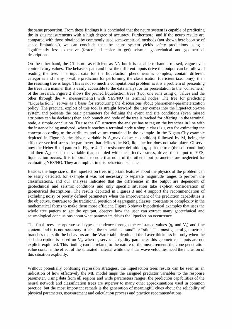
The schematic representation of the liquefaction neuro and tree model is shown in Figure 1. The

following input variables were booked:

1. Geotechnical: Cone penetration resistance “qc_Cone” and the shear wave velocity

“SVelo_Vs”, volumetric weight “Volumetric_W”, type of soil (sand, silt or a mix)

“Soil_Class”, and stresses “Stress_total”, “Stress_effec”,

2. Geometrical: layer thickness “Layer_H”, water level depth “Z_w”, top of layer depth

“Z_TOP”

3. Seismic: moment magnitude “Magnitude_M”, peak ground acceleration “A_max”

Finally, the output variable is “Liquefaction?” and it can take the categorical linguistic values

“YES”/”NO”. By definition, if the factor of safety against triggering liquefaction (FS=CRR/CSR) is

less than 1, the occurrence of YES-liquefaction is predicted and NO-liquefaction is forecasting if

FS≥1. But using ML there are no simple equations for determining the nominal values of CRR and

CSR and the FS.

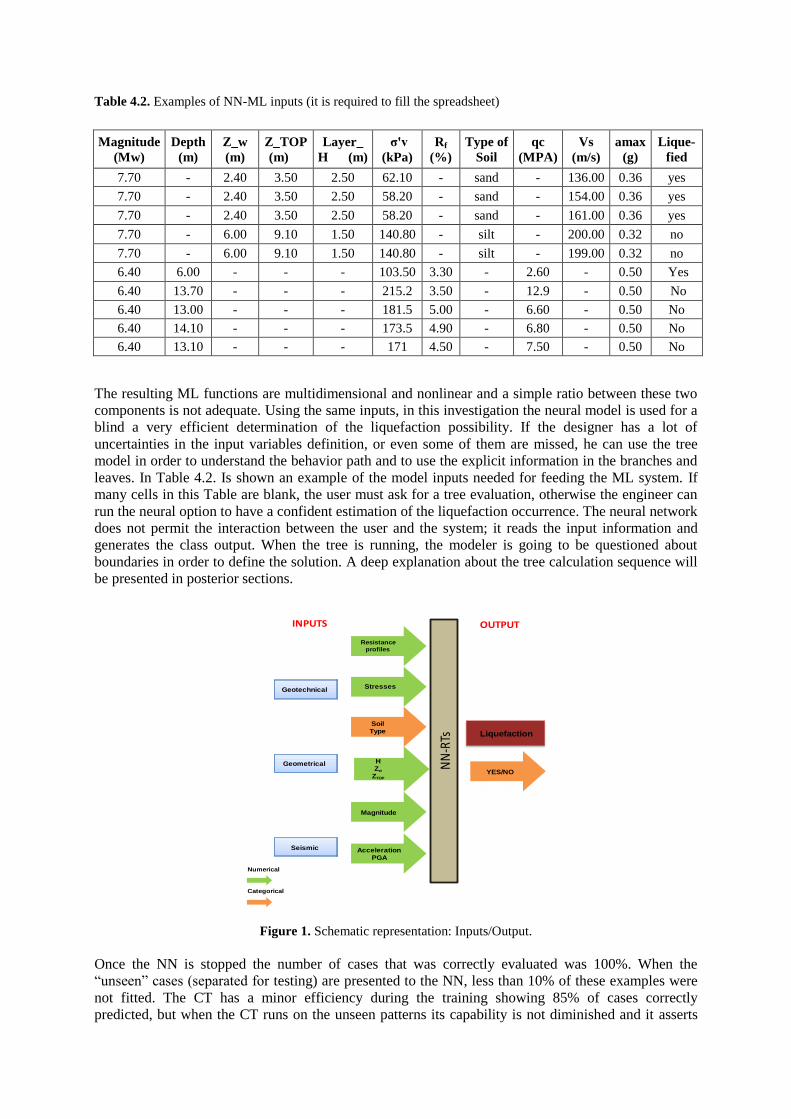
Table 4.2. Examples of NN-ML inputs (it is required to fill the spreadsheet)

Magnitude

(Mw)

Depth

(m)

Z_w

(m)

Z_TOP

(m)

Layer_

H (m)

σ'v

(kPa)

Rf

(%)

Type of

Soil

qc

(MPA)

Vs

(m/s)

amax

(g)

Lique-

fied

7.70 - 2.40 3.50 2.50 62.10 - sand - 136.00 0.36 yes

7.70 - 2.40 3.50 2.50 58.20 - sand - 154.00 0.36 yes

7.70 - 2.40 3.50 2.50 58.20 - sand - 161.00 0.36 yes

7.70 - 6.00 9.10 1.50 140.80 - silt - 200.00 0.32 no

7.70 - 6.00 9.10 1.50 140.80 - silt - 199.00 0.32 no

6.40 6.00 - - - 103.50 3.30 - 2.60 - 0.50 Yes

6.40 13.70 - - - 215.2 3.50 - 12.9 - 0.50 No

6.40 13.00 - - - 181.5 5.00 - 6.60 - 0.50 No

6.40 14.10 - - - 173.5 4.90 - 6.80 - 0.50 No

6.40 13.10 - - - 171 4.50 - 7.50 - 0.50 No

The resulting ML functions are multidimensional and nonlinear and a simple ratio between these two

components is not adequate. Using the same inputs, in this investigation the neural model is used for a

blind a very efficient determination of the liquefaction possibility. If the designer has a lot of

uncertainties in the input variables definition, or even some of them are missed, he can use the tree

model in order to understand the behavior path and to use the explicit information in the branches and

leaves. In Table 4.2. Is shown an example of the model inputs needed for feeding the ML system. If

many cells in this Table are blank, the user must ask for a tree evaluation, otherwise the engineer can

run the neural option to have a confident estimation of the liquefaction occurrence. The neural network

does not permit the interaction between the user and the system; it reads the input information and

generates the class output. When the tree is running, the modeler is going to be questioned about

boundaries in order to define the solution. A deep explanation about the tree calculation sequence will

be presented in posterior sections.

Figure 1. Schematic representation: Inputs/Output.

Once the NN is stopped the number of cases that was correctly evaluated was 100%. When the

“unseen” cases (separated for testing) are presented to the NN, less than 10% of these examples were

not fitted. The CT has a minor efficiency during the training showing 85% of cases correctly

predicted, but when the CT runs on the unseen patterns its capability is not diminished and it asserts

Numerical

Geotechnical

Geometrical

Seismic

Categorical

NN

-RTs Liquefaction

INPUTS OUTPUT

Resistance

profiles

Stresses

SoilType

YES/NO

AccelerationPGA

Magnitude

HZw

ZTOP

the same proportion. From these findings it is concluded that the neuro system is capable of predicting

the in situ measurements with a high degree of accuracy. Furthermore, and if the neuro results are

compared with those obtained by commonly used semi-empirical methods (not shown here because of

space limitations), we can conclude that the neuro system yields safety predictions using a

significantly less expensive (faster and easier to get) seismic, geotechnical and geometrical

descriptions.

On the other hand, the CT is not as efficient as NN but it is capable to handle missed, vague even

contradictory values. The behavior path and how the different inputs drive the output can be followed

reading the tree. The input data for the liquefaction phenomena is complex, contain different

categories and many possible predictors for performing the classification (deficient taxonomy), then

the resulting tree is large. This is not so much a computational problem as it is a problem of presenting

the trees in a manner that is easily accessible to the data analyst or for presentation to the "consumers"

of the research. Figure 2 shows the pruned liquefaction trees (two, one runs using qc values and the

other through the Vs measurements) with YES/NO as terminal nodes. The tree for predicting

“Liquefaction?” serves as a basis for structuring the discussions about phenomena-parameterization

policy. The practical exploit of this tool is straight forward: the user comes into the liquefaction-tree

system and presents the basic parameters for defining the event and site conditions (even missed

attributes can be declared) then each branch and node of the tree is tracked for offering, in the terminal

node, a simple conclusion. To use the CT structure the analyst has to tag on the branches in line with

the instance being analyzed, when it reaches a terminal node a simple class is given for estimating the

concept according to the attributes and values contained in the example. In the Nigata City example

depicted in Figure 3, the driven variable is A_max (seismic condition) followed by M, being the

effective vertical stress the parameter that defines the NO, liquefaction does not take place. Observe

now the Heber Road pattern in Figure 4. The resistance definition qc split the tree (the soil condition)

and then A_max is the variable that, coupled with the effective stress, drives the output to YES,

liquefaction occurs. It is important to note that none of the other input parameters are neglected for

evaluating YES/NO. They are implicit in this behavioral scheme.

Besides the huge size of the liquefaction tree, important features about the physics of the problem can

be easily detected, for example it was not necessary to separate magnitude ranges to perform the

classifications, and our analyses indicated that the differences in the output are dependent of

geotechnical and seismic conditions and only specific situation take explicit consideration of

geometrical descriptions. The results depicted in Figures 3 and 4 support the recommendation of

excluding noisy or poorly defined parameters when the improvement of the prediction capabilities is

the objective, contraire to the traditional position of aggregating classes, constants or complexity in the

mathematical forms to make them more efficient. Figure 5 shows hypothetical examples that uses the

whole tree pattern to get the oputput, observe how the user can extract many geotechnical and

seismological conclusions about what parameters drives the liquefaction occurrence.

The final trees incorporate soil type dependence through the resistance values (qc and Vs) and fine

content, and it is not necessary to label the material as “sand” or “silt”. The most general geometrical

branches that split the behaviors are the Water table depth and the Layer thickness but only when the

soil description is based on Vs, when qc serves as rigidity parameter this geometrical inputs are not

explicit exploited. This finding can be related to the nature of the measurement: the cone penetration

value contains the effect of the saturated material while the shear wave velocities need the inclusion of

this situation explicitly.

Without potentially confusing regression strategies, the liquefaction trees results can be seen as an

indication of how effectively the ML model maps the assigned predictor variables to the response

parameter. Using data from all regions and wide parameters ranges, the prediction capabilities of the

neural network and classification trees are superior to many other approximations used in common

practice, but the most important remark is the generation of meaningful clues about the reliability of

physical parameters, measurement and calculation process and practice recommendations.

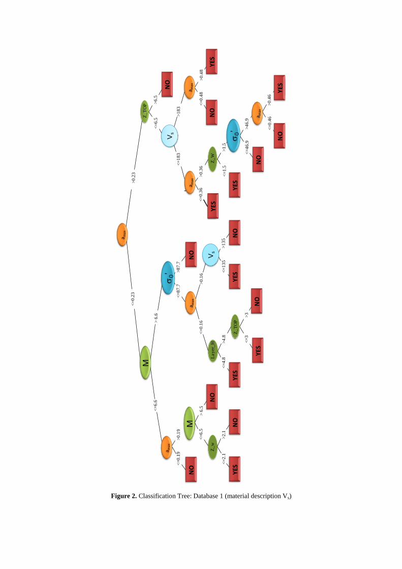
Figure 2. Classification Tree: Database 1 (material description Vs)

Ma

gn

itu

de

no

no

yes

no

Ma

gn

itu

de

no

Z_

w

no

yes

La

yer_

H

yes

Z_

TO

P

yes

no

<=

0.2

3

> 6

.6<

=6

.6

>0

.19

<=

0.1

9

<=

6.5

> 6

.5

<=

2.1

>2

.1

>8

7.7

<=

87

.7

>0

.16

<=

13

5>

13

5

<=

0.1

6

<=

4.8

>4

.8

<=

3>

3

Z_

TO

P

no

<=

6.5

>6

.5

yes

no

yes

Z_

W

yes

<=

18

3>

18

3

<=

0.3

6>

0.3

6<

=0

.48

>0

.48

no

no

yes

<=

1.5

>1

.5

<=

46

.9>

46

.9

<=

0.4

6>

0.4

6

>0

.23

a max

M

a ma

x

a max

a ma

xa m

ax

a ma

x

M

s0’

s0’

Vs

Vs

YES

YES

YES

YES

YES

YES

YES

YESN

O

NO

NO

NO

NO

NO

NO

NO

NO

NO

Figure 2(continue). Classification Tree: Database 2 (material description qc)

qc

no

<=

8.5

>8

.5

Ma

gn

itu

de

no

qc

yes

no

no

yes

no

<=

0.2

<=

6.5

>6

.5

<=

0.1

6>

0.1

6

<=

4.8

>4

.8

<=

2.6

>2

.6

<=

11

6.9

>1

16

.9

qc

yes

z

zn

o

qc

yes

no

yes

yes

no

no

>0

.2

<=

5.4

>5

.4

<=

10

.4>

10

.4

<=

3.8

>3

.8

<=

7.8

>7

.8

<=

0.3

>0

.3

<=

0.2

4>

0.2

4

<=

0.2

2>

0.2

2

qc

NO

NO

NO

NO

NO

NO NO

NO

NO

YES

YES

YES

YES

YES

YES

a ma

x

M

s0’

a max

a ma

x

a ma

x

Rf

Rf

qc

qc

qc

Z T

op

Z To

p

5. CONCLUSIONS

There is a large number of methods that an engineer can select when analyzing classification

problems. Tree techniques, when they “work” and “produce” accurate classifications based on few

logical conditions, have a number of advantages over many of those alternative procedures. In the ML

presented here, there is no implicit assumption that the underlying relationships between the predictor

variables and the dependent variable, follow some specific non-linear link function, or that they are

even monotonic in nature. Thus, ML methods are particularly well suited for seismic data mining

tasks, where there is often little a priori knowledge nor any coherent set of theories or predictions

regarding which variables are related and how. The neural prediction capabilities are remarkable

superior to other conventional models. And the interpretation of behaviors summarized in a

liquefaction tree is very simple. This simplicity is useful not only for purposes of rapid classification

(or prediction) of new observations, but also yield a much simpler model for explaining why

observations are classified or predicted in a particular manner (e.g., to analyze input-output parameters

importance, to present simple statements to management, or to eliminate elaborate and inaccurate

equations). Machine learning represents a powerful alternative in predicting the liquefaction potential

No calibration and normalization with respect to the other parameters is needed. Also the relative

importance of the effective parameters can be compared.

REFERENCES

Andrus, R.D., Stokoe, K.H., II, Chung, R.M., Juang, C.H. (2003), "Guidelines for evaluating liquefaction

resistance using shear wave velocity measurements and simplified procedures." NIST GCR 03-854, National

Institute of Standards and Technology, Gaithersburg, MD.

Andrus, R.D.y Stokoe, K.H., (1996), “Liquefaction Resistance Based on Shear Wave Velocities”, Proc. NCEER

Workshop on Eval. Liquefaction Resistance of Soils, Eds. Youd and Idriss, NCEER-97-0022.

Boulanger, R. and Idriss, I.M. 2004. State normalization of penetration resistance and the effect of overburden

stress on liquefaction resistance. Proc. 11th International Conf. on Soil Dynamics and Earthquake Engineering

and 3rd

International Conference on Earthquake Geotechnical Engineering, Univ. of California, Berkeley, CA.

Garcia, S.R., Romo, M.P., and Ovando-Shelley, E. 2010. ARELI : Árbol de Regresión para Estimar el Potencial

de Licuación. Memorias del Congreso de Mecánica de Suelos, Acapulco, México.

Garcia, S.R., Romo, M.P., and Ovando-Shelley, E. 2011. Machine Learning for Assessing Liquefaction Potential

of Soils. Pan-Am CGS Geotechnical Conference .Canada.

Juang, C. H., Chen, C. J., and Tien, Y. M. 1999. Appraising cone penetration test based liquefaction resistance

evaluation methods: Artificial neural networks approach. Canadian Geotechnical Journal, 36(3) 443-454.

Juang, C. H., Yuan, H. M., Lee, D. H., and Lin 2003, P. S., “Simplified cone penetration test-based method for

evaluating liquefaction resistance of soils,” Journal of Geotechnical and Geoenvironmental Engineering, Vol.

129, No. 1, pp. 66-80.

Kramer S. L., (1996). Geotechnical earthquake engineering. Prentice-Hall International Series in Civil

Engineering and Engineering Mechanics, Prentice Hall, New Jersey, USA.

Youd ,T.L., Idriss, I.M. , Andrus, R.D., Arango, I., Castro, G., Christian, J.T., Dobry, R., Liam F., Harder, L.F.,

Hynes M.E., Ishihara, K., Koester, J.P., Liao,S.S.C., Marcuson III, W.F., Martin, G.R., Mitchell, J.K., Moriwaki,

Y., Power, M.S., Robertson, P.K., Seed, R.B., and Stokoe, K.H. 2001. Liquefaction resistance of soils. Summary

report from the 1996 NCEER and 1998 NCEER/NSF workshops on evaluation of liquefaction resistance of

soils. J. Geotech. Geoenviron. Eng., 127(10), 817–833.

qc

<=8.5

yes

<=0.2

>6.5

<=2.6

<=116.9

Magnitude

amax

s0’

qc

RF

YES

qc (Mpa) 1.4

Vs (m/s) -

ST -

RF (%) 1.3

σ´o (Kpa) 35.9

Z_W (m) -

Z_TOP (m) 3

Layer_H (m) -

M 7.3

a max 0.13

Site

Seismic

Geotechnical

Geometrical

Seismological

Chemical fiber

Heicheng Erathquake 1975

qc

<=8.5

qc

yes

>0.2

<=5.4

qc

YES

qc

amax

qc (Mpa) 2

Vs (m/s) -

ST -

RF (%) 2.8

σ´o (Kpa) 56

Z_W (m) -

Z_TOP (m) 4

Layer_H (m) -

M 6.6

a max 0.8

Site

Seismic

Geotechnical

Geometrical

Seismological

Heber Road

Imperial Valley , 1979

Figure 3. Nigata case: an example of ML Figure 4. Heber Road case: an example of ML

application: NO, liquefaction predicted application: YES, liquefaction predicted

Figure 5. The full connections: an example of reading the branches and nodes

Magnitude

yes

<=0.23

>6.6

>87.7

amax

s0’

NO

qc (Mpa) -

Vs (m/s) 163

ST silt

RF (%) -

σ´o (Kpa) 97.7

Z_W (m) 5

Z_TOP (m) 5

Layer_H (m) 2.5

M 7.5

a max 0.16

Site

Seismic

Geotechnical

Geometrical

Seismological

Nigata

Nigata,Japan 1964

Magnitude

Magnitude

yes

<=0.23

<=6.6

>0.19

<=6.5

<=2.1

amax

amax

Z_W

YES

qc (Mpa) -

Vs (m/s) 124

ST silt

RF (%) -

σ´o (Kpa) 53.9

Z_W (m) 1.5

Z_TOP (m) 2.5

Layer_H (m) 4.3

M 6.5

a max 0.2

Site

Seismic

Geotechnical

Geometrical

Seismological

Wildlife

Superstition Hills C. 1987