Embed Size (px)
Citation preview

School of Electrical Engineering, Computing and
Mathematical Sciences
Link Scheduling in Rechargeable Wireless Sensor
Networks with Limited Harvested Energy
Tony
0000-0002-4284-6587
This thesis is presented for the Degree of
Doctor of Philosophy
of
Curtin University
August 2021


Declaration
To the best of my knowledge and belief this thesis contains no material previously
published by any other person except where due acknowledgment has been made.
This thesis contains no material which has been accepted for the award of any
other degree or diploma in any university.
Signature:
Date: . . . . . . . . . . . . . . . . . . . . . . . . . . . . . . . . . .
iii


“To Lely Hiryanto, Callysta Lie, and Edrick Lie”
“To Wahab Jie, Ervina Teh, Yenti, and Linda”
“To Hiryanto Balok and Mulyati Djaja”
— AUTHOR
v


Abstract
Wireless Sensor Networks (WSNs) have been used in many applications of the
Internet of Things. A well-known issue faced by WSNs is that nodes have limited
energy. To date, rechargeable WSNs (rWSNs) are of great interest because sensor
nodes are able to harvest energy from their environment, e.g., solar and wind,
and store the harvested energy in rechargeable batteries. However, rWSNs have a
number of limitations. First, each node can have a varying energy harvesting time,
i.e., the time required to accumulate energy. Second, the battery characteristics
at each node, which include capacity, leakage rate, and storage efficiency, have
an impact on the operation of rWSNs. Third, the battery suffers from memory
effect if it is partially charged and discharged. Such an effect will decrease the
battery capacity, and thus will eventually shorten its lifetime. The lifetime of the
battery is also affected by the total number of battery charge/discharge cycles.
Another important issue in rWSNs is channel access or link scheduling. This
thesis considers a rWSN that uses a Time Division Multiple Access (TDMA)
link schedule. A TDMA link scheduler ensures packet transmissions in rWSNs
are interference-free. Thus, the energy used for transmission/reception is not
wasted due to interference, which saves energy. A link scheduler is responsible
for determining the set of transmitting and receiving nodes in each time slot. As
the schedule repeats, it is important to minimise the schedule length (in terms of
slots) as this allows nodes to transmit more frequently. Consequently, when links
vii

viii
are activated more frequently, the rWSNs will have a high capacity. However,
in addition to interference, a link scheduler must consider the varying energy
harvesting rates of nodes. More specifically, a link can be activated only if its
end nodes have sufficient energy to transmit/receive packets.
The first part of this thesis focuses on the problem of generating the shortest
TDMA schedule, called Link Scheduling in Harvest Use Store (LSHUS), for use in
rWSNs. This novel problem considers: 1) energy harvesting time, 2) Harvest-Use-
Store protocol that allows the node to use the harvested energy immediately and
stores the remaining energy in its battery for future use, and 3) battery’s capacity,
leakage rate, and storage efficiency. This thesis shows the problem at hand is,
in general, NP-Complete. It presents analytically the optimal schedule for fixed
topologies, e.g., Line, Binary Tree, and Grid. Further, it proposes a greedy
heuristic algorithm, called LS-rWSN, to solve the problem. Our experiments
show that harvesting time, leakage rate, and storage efficiency, significantly affect
the schedule length, whereas battery capacity is an insignificant factor.
The second part of this thesis focuses on another problem of deriving the
TDMA link schedule, called Link Scheduling with Memory Effect-1 (LSME-1),
for rWSNs. This second problem considers: 1) energy harvesting time, 2) Harvest-
Store-Use protocol that requires the harvested energy to be stored in the node’s
battery first before it can be used, 3) battery capacity, leakage rate, and stor-
age efficiency, and 4) a battery cycle constraint which requires the battery to be
charged (discharged) completely before it can be fully discharged (charged) again.
The constraint is used to overcome the memory effect. This thesis shows analyt-
ically: (i) the optimal schedule in fixed topologies, and that (ii) the battery cycle
constraint and leaking batteries can lead to unscheduled links. Further, it de-
scribes a greedy heuristic solution, called LSBCC, that schedules links according
to when their corresponding nodes have sufficient energy. Our simulations show

ix
that enforcing the battery cycle constraint increases the schedule length. On the
other hand, the constraint reduces the number of charge/discharge cycles, and
hence makes the batteries last longer.
The last part of this thesis addresses a problem, called Link Scheduling with
Memory Effect-2 (LSME-2). Problem LSME-2 is an extension of LSME-1 that
considers nodes equipped with a dual-battery system. The dual-battery system
aims to reduce the effect of using the battery cycle constraint on the sched-
ule length. Further, it reduces the number of battery’s charge/discharge cycles.
This thesis presents all possible battery states and transitions for nodes. It then
outlines a greedy algorithm, called LSDBS, to schedule links according to the
earliest time in which batteries at the end nodes of each link can be discharged.
Our results show that equipping nodes with a dual-battery system decreases the
schedule length by up to 35.19% as compared to using a single battery. Such a
system also reduces the number of charge/discharge cycles of the single battery
by up to 13.04%. Finally, a longer energy harvesting time increases link schedules
linearly, but has no impact on the number of charge/discharge cycles.
The performance of all proposed algorithms is evaluated using arbitrary net-
works. The results show the merits and effectiveness of the solutions proposed in
this thesis.


Acknowledgements
This thesis would not have been possible without the support of many people. In
particular, I would like to express my sincere gratitude and thanks to my supervi-
sor, Dr. Sie Teng Soh, for the generous guidance, invaluable advice, support, and
encouragement he has given me throughout my PhD. Without his contribution
in terms of time, ideas, and hard work, I doubt I would have made it halfway
through or achieved any published works. I would also like to express my thanks
to my co-supervisor, Associate Professor Mihai Lazarescu, for his support. In
addition, I am thankful to Associate Professor Kwan-Wu Chin at the University
of Wollongong, for sacrificing his personal time to review and comment on my
papers.
I also want to thank all the anonymous reviewers and editors of conferences
and journals for their time, effort, and comments. Their suggestions have cer-
tainly raised the quality of my publications.
Special thanks must go to the Indonesia Lecturer Scholarship (BUDI) by
Indonesia Endowment Fund for Education (LPDP), Ministry of Finance, Repub-
lic of Indonesia, for the scholarship. I would have been unable to undertake a
PhD without the financial support. Thanks also to the Tarumanagara Univer-
sity, Jakarta, Indonesia, especially the Faculty of Information Technology, for the
support to do this study.
xi

xii
My PhD journey at Curtin University was made wonderful because of the
many friends I have made. Thanks to ISSU Curtin, Julie and Raquel, for their
support during my PhD. Thanks to EECMS staff, Antoni, Robyn, Sucy, Tasneem,
Simret, Ba-Tuong, and Simon, for the help in school administration. Special grat-
itude to Haris Sri Purwoko, Siti Nurlaela, Faiz, Adnan, Debby, Abid Halim, and
Made Andik Setiawan, for their assistance when I first arrived in Perth. Thanks
to Agus, Christofori MRR “Iin” Nastiti, and Cikal, for their friendship. Thanks
to Kalamunda friends, Arnold Kaudin, Rebecca Santi, Sanyulandy Leowalu, Za-
karia Victor Kareth, Benedicta Santoso, and Kemal Faza Hastadi, for all the
joyful conversations. Thanks to Imelda Tandra, Manlika Ratchagit, Kreangkri,
and Suwijak, for the adventurous road trip. Thanks to my English teacher, Elena
and Reva Ramiah for teaching until I achieved the required IELTS score. Thanks
to Josep and Zach in ACE Learning Centre on Lawson Street for countless con-
versations. Thanks also to AIPSSA and BSWA friends, for the opportunities to
contribute. Thanks to my research mates in Building 314 Level 4, Quang, Linh,
Lara, Yuthika, Gaurav, and Suparna, for a pleasant working environment.
Lastly, I am thankful to my wife, Lely Hiryanto, for all her support, for her
cooking, and for loving and taking care of our daughter, Callysta Lie, while I
spent many hours until the middle of many nights and weekends, writing this
thesis and meeting the submission deadlines for conferences and journal papers.

Contents
Abstract vii
Acknowledgements xi
List of Figures xix
List of Tables xxiii
Published Works xxv
Acronyms xxix
Notation xxxi
1 Introduction 1
1.1 Aim and Approach . . . . . . . . . . . . . . . . . . . . . . . . . . 4
1.2 Significance and Contributions . . . . . . . . . . . . . . . . . . . . 5
1.3 Thesis Organisation . . . . . . . . . . . . . . . . . . . . . . . . . . 8
2 Background 11
2.1 Network Model . . . . . . . . . . . . . . . . . . . . . . . . . . . . 11
2.2 Energy Harvesting and Battery Usage Protocols . . . . . . . . . . 13
xiii

Contents xiv
2.3 Interference Models . . . . . . . . . . . . . . . . . . . . . . . . . . 15
2.4 MAC Layer . . . . . . . . . . . . . . . . . . . . . . . . . . . . . . 17
2.5 Related Works . . . . . . . . . . . . . . . . . . . . . . . . . . . . . 18
2.6 Simulation Environments . . . . . . . . . . . . . . . . . . . . . . . 21
2.6.1 Topologies . . . . . . . . . . . . . . . . . . . . . . . . . . . 21
2.6.1.1 Fixed Topologies . . . . . . . . . . . . . . . . . . 21
2.6.1.2 Arbitrary Network . . . . . . . . . . . . . . . . . 23
2.6.2 Platform . . . . . . . . . . . . . . . . . . . . . . . . . . . . 24
2.7 Chapter Summary . . . . . . . . . . . . . . . . . . . . . . . . . . 24
3 Link Scheduling in rWSNs with Harvesting Time and Battery
Capacity Constraints 25
3.1 Preliminaries . . . . . . . . . . . . . . . . . . . . . . . . . . . . . 28
3.1.1 Network Model . . . . . . . . . . . . . . . . . . . . . . . . 28
3.1.2 Problem Statement . . . . . . . . . . . . . . . . . . . . . . 30
3.1.3 Problem Analysis . . . . . . . . . . . . . . . . . . . . . . . 34
3.2 Solution . . . . . . . . . . . . . . . . . . . . . . . . . . . . . . . . 38
3.2.1 Key Properties . . . . . . . . . . . . . . . . . . . . . . . . 38
3.2.2 LS-rWSN . . . . . . . . . . . . . . . . . . . . . . . . . . . 43
3.3 Evaluation . . . . . . . . . . . . . . . . . . . . . . . . . . . . . . . 46
3.3.1 HSU versus HUS . . . . . . . . . . . . . . . . . . . . . . . 47
3.3.2 Effect of ri, µi, and ηi on |S| . . . . . . . . . . . . . . . . . 49
3.3.2.1 Effect of Harvesting Time . . . . . . . . . . . . . 50
3.3.2.2 Effect of Leakage Rate . . . . . . . . . . . . . . . 50

xv Contents
3.3.2.3 Effect of Storage Efficiency . . . . . . . . . . . . 51
3.3.2.4 Effect of Leakage Rate and Storage Efficiency . . 52
3.3.3 Effect of bi, µi, and ηi on |S| . . . . . . . . . . . . . . . . . 54
3.3.3.1 Effect of Battery Capacity . . . . . . . . . . . . . 54
3.3.3.2 Effect of Leakage Rate . . . . . . . . . . . . . . . 55
3.3.3.3 Effect of Storage Efficiency . . . . . . . . . . . . 56
3.3.4 Effectiveness of LS-rWSN . . . . . . . . . . . . . . . . . . 57
3.3.4.1 Fixed Topologies . . . . . . . . . . . . . . . . . . 57
3.3.4.2 Arbitrary Networks . . . . . . . . . . . . . . . . . 58
3.3.5 Running Time . . . . . . . . . . . . . . . . . . . . . . . . . 60
3.4 Chapter Summary . . . . . . . . . . . . . . . . . . . . . . . . . . 60
4 Link Scheduling in rWSNs with Battery Memory Effect 63
4.1 Preliminaries . . . . . . . . . . . . . . . . . . . . . . . . . . . . . 65
4.1.1 Network Model . . . . . . . . . . . . . . . . . . . . . . . . 66
4.1.2 Problem Statement . . . . . . . . . . . . . . . . . . . . . . 69
4.1.3 Problem Analysis . . . . . . . . . . . . . . . . . . . . . . . 70
4.2 Solution . . . . . . . . . . . . . . . . . . . . . . . . . . . . . . . . 74
4.2.1 Key Properties . . . . . . . . . . . . . . . . . . . . . . . . 74
4.2.2 Problem Solution Feasibility . . . . . . . . . . . . . . . . 86
4.2.3 A Method to Shorten Superframe Length . . . . . . . . . . 90
4.2.4 LSBCC . . . . . . . . . . . . . . . . . . . . . . . . . . . . 91
4.3 Evaluation . . . . . . . . . . . . . . . . . . . . . . . . . . . . . . . 96
4.3.1 Battery with No Leakage . . . . . . . . . . . . . . . . . . . 98

Contents xvi
4.3.1.1 LSBCC versus LSNBC . . . . . . . . . . . . . . . 98
4.3.1.2 Effect of Harvesting Time . . . . . . . . . . . . . 99
4.3.1.3 Effect of Battery’s DoD . . . . . . . . . . . . . . 101
4.3.2 Feasible Solutions of LSME-1 . . . . . . . . . . . . . . . . 104
4.3.2.1 Same Parameter Values . . . . . . . . . . . . . . 104
4.3.2.2 Random Parameter Values . . . . . . . . . . . . . 105
4.3.2.3 Different Values of µi . . . . . . . . . . . . . . . . 105
4.3.2.4 Different Values of ri . . . . . . . . . . . . . . . . 106
4.3.2.5 Different Values of Pair (ri, µi) . . . . . . . . . . 106
4.3.3 Leak-Free versus Leaky Battery . . . . . . . . . . . . . . . 107
4.3.3.1 LSBCC versus LSNBC . . . . . . . . . . . . . . . 108
4.3.3.2 Charging versus Discharging Constraint . . . . . 110
4.3.3.3 Charge/Discharge Cycles . . . . . . . . . . . . . 111
4.3.4 Effectiveness of LSBCC . . . . . . . . . . . . . . . . . . . 113
4.4 Chapter Summary . . . . . . . . . . . . . . . . . . . . . . . . . . 114
5 Link Scheduling in rWSNs with a Dual-Battery System 115
5.1 Preliminaries . . . . . . . . . . . . . . . . . . . . . . . . . . . . . 117
5.1.1 Network Model . . . . . . . . . . . . . . . . . . . . . . . . 118
5.1.2 Problem Statement . . . . . . . . . . . . . . . . . . . . . . 120
5.2 Solution . . . . . . . . . . . . . . . . . . . . . . . . . . . . . . . . 121
5.2.1 Battery States and Transitions . . . . . . . . . . . . . . . 121
5.2.2 Key Properties . . . . . . . . . . . . . . . . . . . . . . . . 124
5.2.3 LSDBS . . . . . . . . . . . . . . . . . . . . . . . . . . . . . 126

xvii Contents
5.3 Evaluation . . . . . . . . . . . . . . . . . . . . . . . . . . . . . . . 129
5.3.1 Effect of Battery Cycle Constraint . . . . . . . . . . . . . 129
5.3.2 Effect of Harvesting Time . . . . . . . . . . . . . . . . . . 132
5.4 Chapter Summary . . . . . . . . . . . . . . . . . . . . . . . . . . 134
6 Conclusion 135
6.1 Summary . . . . . . . . . . . . . . . . . . . . . . . . . . . . . . . 135
6.2 Future Work . . . . . . . . . . . . . . . . . . . . . . . . . . . . . . 138
Appendix
Copyright Information 141
Bibliography 155


List of Figures
2.1 Interference models [1]. . . . . . . . . . . . . . . . . . . . . . . . . 16
2.2 A line graph with eight nodes. . . . . . . . . . . . . . . . . . . . . 22
2.3 A binary tree with four levels. . . . . . . . . . . . . . . . . . . . . 23
2.4 A (4×3) grid. . . . . . . . . . . . . . . . . . . . . . . . . . . . . . 24
3.1 An example (a) with only protocol interference constraint, and (b)
with protocol interference, harvesting time, and battery capacity
constraints. . . . . . . . . . . . . . . . . . . . . . . . . . . . . . . 27
3.2 A rWSN model: (a) graph G, and its (b) conflict graph CG. . . . 31
3.3 TDMA schedules for the rWSN in Figure 3.2. . . . . . . . . . . . 31
3.4 An instance of (a) graph G, and its mapping (b) graph G′. . . . . 34
3.5 HUS versus HSU in rWSNs of 50 nodes. . . . . . . . . . . . . . . 48
3.6 The effect of energy unavailability on |S|. . . . . . . . . . . . . . . 49
3.7 The effect of harvesting time and leakage rate on |S|. . . . . . . . 51
3.8 The effect of harvesting time and storage efficiency on |S|. . . . . 53
3.9 Effect of network sizes with varying ri on |S|. . . . . . . . . . . . 54
3.10 The effect of battery capacity and leakage rate in a rWSN with 40
nodes. . . . . . . . . . . . . . . . . . . . . . . . . . . . . . . . . . 56
xix

List of Figures xx
3.11 The effect of battery capacity and storage efficiency in a network
with 40 nodes. . . . . . . . . . . . . . . . . . . . . . . . . . . . . 57
3.12 The performance of LS-rWSN in fixed topologies with a various
number of nodes for µi = 0 and ηi = 1. . . . . . . . . . . . . . . . 58
3.13 The performance of LS-rWSN in arbitrary networks for µi = 0.01
and ηi = 0.7. . . . . . . . . . . . . . . . . . . . . . . . . . . . . . 59
3.14 The running time of LS-rWSN in arbitrary networks for ri = 10,
µi = 0.01, and ηi = 0.7. . . . . . . . . . . . . . . . . . . . . . . . . 59
4.1 An example (a) with interference and harvesting time, (b) plus
battery capacity, and (c) plus battery cycle constraints. . . . . . . 64
4.2 Charge-discharge cycles at a node vi at cycle k = 1 and k = 2. . . 67
4.3 A rWSN as a (a) graph G, and its (b) conflict graph CG. . . . . . 69
4.4 TDMA link schedules for the rWSN in Figure 4.3 with a battery
cycle constraint. . . . . . . . . . . . . . . . . . . . . . . . . . . . . 69
4.5 An illustration for Propositions 4.9 and 4.10. . . . . . . . . . . . . 81
4.6 An illustration for Eq. (4.24) to Eq. (4.27). . . . . . . . . . . . . . 83
4.7 Two scenarios to schedule a link li,j. . . . . . . . . . . . . . . . . . 83
4.8 A discharging cycle of the battery at node vi (top) and vj (bottom). 85
4.9 A cycle with three nodes. . . . . . . . . . . . . . . . . . . . . . . . 89
4.10 LSBCC versus LSNBC in terms of |S|. . . . . . . . . . . . . . . . 99
4.11 LSBCC versus LSNBC on charge/discharge cycles. . . . . . . . . 100
4.12 Effect of harvesting time ri on |S|. . . . . . . . . . . . . . . . . . 101
4.13 Effect of battery’s DoD on |S|. . . . . . . . . . . . . . . . . . . . . 103
4.14 Effect of battery’s DoD on charge/discharge cycles. . . . . . . . . 103

xxi List of Figures
4.15 LSBCC versus LSNBC in networks where each node has a leak-free
or a leaky battery in terms of |S|. . . . . . . . . . . . . . . . . . . 110
4.16 LSCC versus LSDC in networks where each node has a leak-free
or a leaky battery in terms of |S|. . . . . . . . . . . . . . . . . . . 111
4.17 LSBCC versus LSNBC in networks where each node has a leak-free
or a leaky battery in terms of the number of charge/discharge cycles.112
4.18 The performance of LSBCC in fixed topologies with a various num-
ber of nodes for µi = 0 and ηi = 1. . . . . . . . . . . . . . . . . . 113
5.1 A sensor node with a dual-battery system. . . . . . . . . . . . . . 115
5.2 An example for (a) single battery without battery cycle constraint,
(b) single battery with battery cycle constraint, (c) dual battery
with battery cycle constraint. . . . . . . . . . . . . . . . . . . . . 117
5.3 A rWSN model: (a) graph G, and its (b) conflict graph CG. . . . 120
5.4 TDMA link schedules for the rWSN depicted in Figure 5.3. . . . . 121
5.5 LSDBS, LSBCC, LSNBC on |S|. . . . . . . . . . . . . . . . . . . 131
5.6 LSDBS, LSBCC, LSNBC on charge/discharge cycles. . . . . . . . 132
5.7 Effect of harvesting time ri on |S|. . . . . . . . . . . . . . . . . . 133


List of Tables
2.1 Specifications of rechargeable batteries [2]. . . . . . . . . . . . . . 14
3.1 Parameter values used in the evaluation. . . . . . . . . . . . . . . 47
4.1 Parameter values used in our evaluation. . . . . . . . . . . . . . . 97
4.2 The number of scheduled links (in %). . . . . . . . . . . . . . . . 104
4.3 Superframe length |S| of LSBCCf and LSBCCnf . . . . . . . . . . 108
5.1 States and transitions of batteries at each node vi. . . . . . . . . . 123
5.2 Parameter values used in the evaluation. . . . . . . . . . . . . . . 129
6.1 Three link scheduling problems with proposed solutions, constraints,
battery usage protocol, and the number of batteries per node. . . 135
xxiii


Published Works
This thesis is based upon several works that have been presented at conferences
and published in journals over the course of the author’s PhD. They are listed as
follows in chronological order:
1. Tony, Sieteng Soh, Kwan-Wu Chin, Mihai Lazarescu, “Link Scheduling in
Rechargeable Wireless Sensor Networks with Harvesting Time and Battery
Constraints,” in 43rd IEEE Conference on Local Computer Networks (LCN),
Chicago, IL, USA, Oct., 2018. The paper received the Student Participation
Grant. It is part of Chapter 3.
2. Tony Tony, Sieteng Soh, Kwan-Wu Chin, Mihai Lazarescu,“Link Schedul-
ing in Rechargeable Wireless Sensor Networks with Imperfect Batteries,”
in IEEE Access, vol. 7, pp. 104721−104736, 2019. The paper is part of
Chapter 3.
3. Tony Tony, Sieteng Soh, Kwan-Wu Chin, Mihai Lazarescu,“Link Schedul-
ing in Rechargeable Wireless Sensor Networks with Battery Memory Ef-
fects,” in 30th International Telecommunication Networks and Applications
Conference (ITNAC), Melbourne, Australia, Nov., 2020. The paper re-
ceived the Student Travel Grant and Best Student Paper. It is part of
Chapter 4.
xxv

xxvi
4. Tony Tony, Sieteng Soh, Kwan-Wu Chin, Mihai Lazarescu,“Link Schedul-
ing in Rechargeable Wireless Sensor Networks with Imperfect Battery and
Memory Effects,” in IEEE Access, vol. 9, pp. 17803−17819, 2021. The
paper is part of Chapter 4.
5. Tony Tony, Sieteng Soh, Kwan-Wu Chin, Mihai Lazarescu,“Link Schedul-
ing in Rechargeable Wireless Sensor Networks with a Dual-Battery Sys-
tem,” in IEEE International Conference on Communications (ICC), Mon-
treal, Canada, Jun. 2021. The paper received the Student Grant. It is part
of Chapter 5.
I have obtained permission from the copyright owners to use any of my own
published works in which the copyright is held by another party (publisher and
co-author). The copyright information to reuse the published works has been
provided in Appendix. Table 1 shows an attribution statement for all published
works.

xxvii


Acronyms
WSNs Wireless Sensor NetworksIoTs Internet of ThingsrWSNs rechargeable Wireless Sensor NetworksWPT Wireless Power TransferDoD Depth of DischargeTDMA Time Division Multiple AccessMAC Medium Access ControlCSMA Carrier Sense Multiple AccessPOMDP Partially Observable Markov Decision ProcessEH Energy HarvestingRF Radio FrequencyHU Harvest UseHSU Harvest Store UseHUS Harvest Use StoreRTS Request To SendCTS Clear To SendLSHUS Link Scheduling in Harvest Use StoreLSME-1 Link Scheduling with Memory Effect-1LSME-2 Link Scheduling with Memory Effect-2LS-rWSN Link Scheduler for a rechargeable Wireless Sensor NetworkLSBCC Link Scheduler with Battery Cycle ConstraintLSNBC Link Scheduler with No Battery Cycle ConstraintLSCC Link Scheduler with Charging ConstraintLSDC Link Scheduler with Discharging ConstraintLSDBS Link Scheduler with a Dual-Battery System
xxix


Notation
Notation DefinitionG(V,E) A directed graph with |V | nodes and |E| links.CG(V ′, E ′) A conflict graph for a graph G(V,E).
V The set of sensor nodes.vi A sensor node i.E The set of directional links.li,j A directed link from node vi to node vj.wi,j The link weight for each incident link li,j at a node vi.Ri The transmission range of each node vi.ri Time for the harvester in a node vi to accumulate 1ε unit of energy.bi The battery capacity of a node vi.µi The battery leakage rate of a node vi.ηi The battery storage efficiency of a node vi.bi,t The battery level of a node vi at time t.Ai,t The amount of energy that a node vi can use at time t.ti The most recent time the battery at a node vi was used.τi The time span between time ti and t, i.e., τi = t− ti.ρi When Ai,ti < 1, ρi = t− ti is the amount of time (in slots) for a node
vi to accumulate energy such that Ai,t ≥ 1.ti,j The earliest time in which the end nodes of a link (i, j) have sufficient
energy.αi,t A binary variable that indicates whether a node vi is able to trans-
mit/receive one packet at time t.Ti The earliest timeslot when a node vi has sufficient energy to trans-
mit/receive one packet.
bi,t The energy level of the battery in charging mode at a node vi at timeslot t.
bi,max The upper limit capacity of the battery at a node vi.bi,min The lower limit capacity of the battery at a node vi.
xxxi

xxxii
Notation Definition
bi The battery usable energy at a node vi.t+i,k The start time of charging cycle k of the battery at a node vi.
t−i,k The end time of charging cycle k of the battery at a node vi.
t+i,k The start time of discharging cycle k of the battery at a node vi.
t−i,k The end time of discharging cycle k of the battery at a node vi.
τi,k The charging time interval of the battery at a node vi at cycle k ≥ 1.τi,k The discharging time interval of the battery at a node vi at cycle
k ≥ 1.bi,ti The energy level of the battery at a node vi at timeslot ti.σi,ti A binary variable that indicates whether the battery at a node vi can
be discharged at time ti.Ti,k The latest timeslot when the battery at a node vi can be discharged
in a discharging cycle k.Bzi The dual battery at a node vi for z ∈ {1, 2}.
B1i The first battery at a node vi.
B2i The second battery at a node vi.bzi The capacity of the battery z at a node vi.
bzi Each battery’s usable energy.tz+i The start charging time of the battery z at a node vi.tz−i The end charging time of the battery z at a node vi.tz+i The start discharging time of the battery z at a node vi.tz−i The end discharging time of the battery z at a node vi.τ zi The charging time interval of the battery z at a node vi.τ zi The discharging time interval of the battery z at a node vi.
bzi,t The amount of energy stored in the battery z at a node vi at the startof slot t for a charging cycle.
bzi,t The amount of energy stored in the battery z at a node vi at the startof slot t for a discharging cycle.
|S| The superframe or schedule length.τ The length of each timeslot.ε Energy needed to transmit/receive a packet.

Chapter 1
Introduction
Wireless Sensor Networks (WSNs) are of great interest to the Internet of Things
(IoTs) community [3]. They have been used in many applications [4], e.g.,
military [5], habitat [6][7][8] or environment [9][10][11][12][13], health [14][15],
home [16][17][18][19], industry [20][21][22], and commercial applications [23]. They
consist of various numbers (tens to thousands) of small devices (nodes) embed-
ded with sensors that have the ability to collect useful information from their
surroundings and forward it to one or more base/central/sink locations via wire-
less communications [24][25][26]. Each sensor node is composed of four subsys-
tems [27]: (i) sensing unit to collect data, (ii) processing unit to deal with data,
(iii) wireless communication unit to transfer data, and (iv) power unit to activate
the sensor node.
A well-known issue faced by WSNs is that nodes have limited energy. In some
implementations, it is impractical to replace the batteries of nodes due to energy
depletion, especially when there are a large number of sensor nodes and they
are deployed in difficult-to-reach locations. Based on the battery type used by
their sensor nodes, WSNs can be classified into two categories: non-rechargeable
and rechargeable. The non-rechargeable WSNs will stop their operations once
1

2
the batteries are depleted−each battery has only a limited amount of energy. To
maximise the battery’s lifetime, researchers have proposed various techniques,
e.g., energy-efficient link scheduling and routing protocols [28] that minimise en-
ergy usage while optimising network quality of service (QoS), e.g., throughput,
delay, and fairness. In contrast, the rechargeable WSNs (rWSNs) use batteries
that can be recharged by harvesting energy from their environment, e.g., solar,
wind, and/or some types of wireless power transfer (WPT) techniques [29], such
as Witricity [30]. Thus, rWSNs potentially can be immortal [31]. Nevertheless,
those energy-efficient techniques are still relevant in the context of rWSNs due to
limited energy sources by the existing energy harvesting technology and limited
battery capacity.
To this end, rWSNs are now of great interest because sensor nodes are able
to harvest energy from their environment. However, they have a number of
operational issues. First, the energy arrivals of nodes exhibit spatio-temporal
properties. This means nodes may experience time-varying energy arrivals. When
a node exhausts its energy, it will have to spend time for harvesting energy before
it continues executing tasks. Thus, a node that has a greater energy consumption
rate than its energy harvesting rate can operate perpetually, but with delays.
The time used to harvest a given amount of energy is affected by the type of
energy source as well as a node’s location [32]. For instance, assuming a solar
panel has a power density of 15, 000 µW/cm3 and 20 µW/cm3 for outdoor and
indoor settings, respectively [33], hence, a node with a 50 cm3 solar panel will
have a corresponding energy harvesting rate of 300 mJ/s (outdoor) and 0.4 mJ/s
(indoor). A Mica2 mote [34], which requires 30 mJ of energy to transmit/receive
a packet, will need to spend 0.1s (outdoor) or 75s (indoor) for harvesting energy
before it can transmit/receive one packet.
3
The second important issue of interest recently is the lifetime of rechargeable
batteries. Among others, one contributing factor to the battery’s lifetime is mem-
ory effect [35], which decreases its usable capacity if the battery is charged and
discharged repeatedly, after a partial discharge and charge, respectively. This
degradation can be avoided by enforcing a so-called battery cycle constraint, i.e.,
a node must charge (or discharge) its battery completely before fully discharging
(or charging) its battery again [36]. In addition, the degradation can be reduced
by equipping the rWSNs with a dual-battery system [37], in which the batter-
ies are charged and discharged alternately. Another factor is the percentage of
discharged energy relative to a battery’s overall capacity which is also called as
battery’s Depth of Discharge (DoD) [38]. Further, frequent charging and dis-
charging also affects a battery’s lifetime [39].
The third issue is channel access or link scheduling [40], which determines
when nodes activate their link(s), and thus governs the network capacity of an
rWSN. To this end, this thesis considers Time Division Multiple Access (TDMA)
to ensure that nodes do not experience collisions nor waste energy, and that
they only need to be active during the allocated timeslot. Specifically, a link
scheduler is responsible for determining the set of transmitting and receiving
nodes in each time slot. As the TDMA schedule repeats, it is important that
the schedule length (in terms of slots) is short as this allows nodes to transmit
frequently; consequently, as links are activated frequently, they will have a high
capacity. The schedule governs the active time of a node; therefore, a node
only needs to become active if its neighbours are active. In other words, such
schedule minimises idle listening [41]. It is evident that a link scheduler plays
a critical role in an rWSN. Past works on link scheduling assumed nodes have
no energy harvesting constraint [42]. In contrast, in an rWSN, link schedulers
must consider the varying energy harvesting rates of sensor nodes. Specifically,

1.1. Aim and Approach 4
they must consider the energy harvesting time of nodes, i.e., the time interval in
which a sensor node accumulates sufficient energy to either transmit/receive a
packet. Without this consideration, a link scheduler may allocate slots to nodes
that have insufficient energy to transmit/receive a packet. Another important
factor to consider are battery characteristics, namely: (i) limited capacity, i.e.,
battery capacity, (ii) leakage, and (iii) storage efficiency. These characteristics
can result in a longer link schedule. Our work in this thesis considers all of the
above factors. It is important to note that link scheduling problem in general
is known to be NP-hard [43]. Further, our problem is the general version of the
link scheduling problem that assumes nodes have no energy constraint. Thus, all
problems addressed in this thesis are in NP-hard.
Our research hypothesis are as follows: (i) the harvesting time can signifi-
cantly effect the link schedule; as each node has to wait for its harvesting time
to accumulate sufficient energy before it can transmit/receive a packet, (ii) the
imperfect battery characteristics can lead to a longer link schedule; since the bat-
tery will take longer time to have energy due to leakage and/or storage efficiency,
and (iii) the battery cycle constraint can significantly increase the link schedule
length; the reason is the battery can only be charged (discharged) if its energy
level reaches the minimum (maximum) level.
1.1 Aim and Approach
The aims of our works are as follows.
Aim 1 − To propose and analyse a novel TDMA link scheduling problem for
rWSNs with energy harvesting time and battery capacity constraints. This thesis
proposes a heuristic approach, called Link Scheduler in a rechargeable Wireless
Sensor Network (LS-rWSN). The greedy approach selects non-interfering links

5 1.2. Significance and Contributions
starting from the link whose end nodes have sufficient energy to transmit/receive
one packet at the earliest time.
Aim 2 − To propose and analyse a novel TDMA link scheduling problem for
rWSNs that consider battery memory effect. Note that this problem extends
that in Aim 1 to reduce the impact of memory effect that is caused by repeated
charge/discharge cycles of batteries. Our proposed heuristic approach, called Link
Scheduler with Battery Cycle Constraint (LSBCC), requires each battery to be
charged (discharged) completely before it can be discharged (charged) again. In
addition, the greedy heuristic schedules all non-interfering links at the earliest
possible timeslot when the batteries at their end nodes can be used.
Aim 3 − To propose and analyse a novel problem to reduce the negative effect of
enforcing the battery cycle constraint of Aim 2 on a TDMA link schedule length.
Our proposed approach, called Link Scheduler with a Dual-Battery System (LS-
DBS), uses a dual-battery system; each of which is subjected to the battery cycle
constraint. Further, the heuristic greedily schedules all non-interfering links at
the earliest possible timeslot.
Our proposed link schedulers, i.e., LS-rWSN, LSBCC, and LSDBS, are to be
deployed in a centralised manner.
1.2 Significance and Contributions
The main significance and contributions of this thesis are threefold.
1. It addresses a novel TDMA link scheduling problem, called Link Scheduling
in Harvest-Use-Store (LSHUS), and proposes a solution called LS-rWSN,

1.2. Significance and Contributions 6
to maximise the throughput of rWSNs where: (i) sensor nodes have differ-
ent energy harvesting times, (ii) sensor nodes have a battery with a finite
capacity, and each battery has a less-than-ideal storage efficiency and leaks
over time, and (iii) each link i has a weight wi ≥ 1 that specifies that it
must be scheduled at least wi times in the resulting schedule. To the best
of our knowledge, no link schedulers have simultaneously considered fac-
tors (i)-(iii). The authors of [44] considered factors (i) and (iii) and they
assumed nodes used the Harvest-Store-Use (HSU) model with unlimited
battery capacity. More specifically, the work in [44] assumed batteries that
were leakage free and had 100% storage efficiency. This thesis, particularly
Chapters 3 and 4, also consider different leakage rates and storage effi-
ciencies. Furthermore, it outlines an efficient greedy technique to generate
TDMA link schedules and contains analysis of its time complexity. In ad-
dition, it presents proof to show that LSHUS is NP-Complete and contains
analysis of the optimal schedule length for the following topologies: Line,
Tree, and Grid. The proposed technique does not require an extended con-
flict graph, as in [44], and thus, it is more efficient. The results in Chapter 3
show that imperfect batteries increase the schedule length. The conclusion
is justified by our simulation results in Chapter 3.
2. It presents a TDMA link scheduling problem, called Link Scheduling with
Memory Effect-1 (LSME-1), that considers: (i) sensor nodes with different
energy harvesting times and a finite battery capacity, (ii) battery operation
governed by a battery cycle constraint, (iii) batteries with a leakage rate and
storage efficiency, and (iv) activation of each link (i, j) at least wi,j times. It
analyses the optimal schedule length for three fixed topologies: Line, Tree,
and Grid. Further, it develops a novel heuristic technique, called LSBCC,
7 1.2. Significance and Contributions
that greedily schedules links that can be activated according to when their
end nodes are able to transmit/receive a packet. In addition, it analyti-
cally shows that some links cannot be scheduled for networks that contain
batteries with a non-negative leakage rate. This conclusion is supported by
our simulation results in Chapter 4.
3. It proposes a new TDMA link scheduling problem, called LSME-2, to max-
imise throughput in rWSNs where: (i) sensor nodes have a different energy
harvesting time, (ii) each node is equipped with a dual-battery system, (iii)
each battery has a finite capacity, (iv) each battery has a battery cycle con-
straint, and (v) each link i has a weight wi ≥ 1 and must be scheduled
at least wi times. It presents battery states and their state transitions in
the dual-battery system. Further, it develops a heuristic algorithm called
LSDBS, to generate a TDMA link schedule, where it schedules links that
can be activated at the earliest time when one of the dual battery at their
end nodes can be discharged to transmit/receive a packet. The simulation
results in Chapter 5 show that using two batteries at each node reduces the
schedule length and number of battery charge/discharge cycles.
The impact of our research projects in this thesis are as follows: (i) the eco-
nomic impact: our work contributes to decreasing the energy cost as it utilizes
energy harvesting, (ii) the environmental impact: since our research is related
to renewable energy, it helps to reduce global greenhouse gas emission [45], and
(iii) the research communities impact: this work has a potential interdisciplinary
research collaboration.

1.3. Thesis Organisation 8
1.3 Thesis Organisation
The contents of each chapter in this thesis are as follows.
Chapter 2: Background
Chapter 2 discusses the background, network model, and notations that are used
in this thesis. It describes three protocols of energy harvesting and battery usage.
Further, it addresses interference models. It covers an overview of TDMA link
scheduling. A review of related works on link scheduling problems is also dis-
cussed. Lastly, the chapter presents the simulation environment used to evaluate
the performance of all proposed algorithms in this thesis.
Chapter 3: Link Scheduling in rWSNs with Harvesting Time and Bat-
tery Capacity Constraints
Chapter 3 formally defines the LSHUS problem and describes our proposed solu-
tion to the problem, i.e., LS-rWSN. The chapter includes a proof of the problem
and the analytical analysis of optimal schedule length for three fixed topologies.
Finally, the chapter evaluates our LS-rWSN algorithm using simulation.
Chapter 4: Link Scheduling in rWSNs with Battery Memory Effect
Chapter 4 formulates the LSME-1 problem and presents our proposed solution,
i.e., LSBCC. This chapter presents analytically the optimal schedule length for
fixed topologies. It also shows the feasibility study of LSME-1. Finally, Chapter 4
includes simulations to evaluate the LSBCC algorithm.

9 1.3. Thesis Organisation
Chapter 5: Link Scheduling in rWSNs with a Dual-Battery System
Chapter 5 addresses the LSME-2 problem and shows our proposed solution, i.e.,
LSDBS. The chapter describes battery states and state transitions in a dual-
battery system. We perform simulations to evaluate our solution.
Chapter 6: Conclusion
Chapter 6 summarises this thesis and discusses possible areas of future research.
This thesis includes one Appendix that contains copyright information from
IEEE conferences and journals in which the author has published.


Chapter 2
Background
This chapter is divided into seven sections. It contains all the theory and materials
that are used in Chapters 3, 4, and 5. Section 2.1 describes the network model
and notations that are used throughout this thesis. Additional notations that are
used only in specific chapters will be described in their corresponding chapters.
Section 2.2 discusses energy harvesting and battery usage protocols. Section 2.3
introduces interference models for WSNs. Section 2.4 addresses an overview of
MAC layer, including TDMA link scheduling. Section 2.5 reviews the literature
related to this thesis. Section 2.6 presents the network topologies and platform
used in the thesis. Finally, Section 2.7 summarises this chapter.
2.1 Network Model
A rWSN is modelled as a directed graph G(V,E), where each node vi ∈ V is
a sensor node and each link li,j ∈ E denotes a directed link from node vi to
node vj. Each node vi has a transmission range of Ri. Let ||vi − vj|| be the
Euclidean distance between nodes vi and vj. A node vi can transmit/receive
packets to/from node vj if ||vi − vj|| ≤ Ri. Each link li,j ∈ E has weight of
11

2.1. Network Model 12
wi,j ≥ 1, meaning the link must be activated at least wi,j times in the generated
schedule to transmit/receive data packets in networks with continuous traffic
model. We assume each node has a fixed location in a network.
A sensor node consumes energy when sensing the environment, computing
collected samples, and communicating with its neighbours, which includes trans-
mitting, receiving, listening for messages on the radio channel, sleeping, and
switching state [46]. This work assumes that communication is the only source
of energy expenditure. The assumption is reasonable because as shown in [46],
the energy consumption of nodes for communications is significantly larger than
the other operations, e.g., 180.10 mJ, 17.242 mJ, and 5.2 mJ for communication,
sensing, and computing, respectively. Similar to [47], we assume the energy usage
for transmission and reception is equal. Let ε (in Joule) be the energy consumed
when transmitting or receiving one packet. For example, assuming a TI CC2420
transceiver uses 226 nJ/bit for transmission [48] and a packet size of 125 bytes
or 1,000 bits, then we have ε = 226 µJ.
A node vi is equipped with a harvester that scavenges energy from its envi-
ronment, e.g., solar, and a rechargeable battery with capacity of bi (in a unit of
ε). Note that our work does not make any specific assumption about any energy
harvesting model used by nodes; i.e., the problem is independent of any specific
energy harvesting model. That is, it assumes each node has a known energy
arrival rate that arrives after energy conversion. In addition, it is independent
of any specific signal propagation models and spread spectrum technology. Let
ri ≥ 1 (in slots) be the harvesting time or total number of slots that is required
by a node vi to accumulate 1ε of energy. Thus, the harvesting rate of a node
vi is εri
per time slot. Let 0 < ηi ≤ 1 be the storage efficiency and 0 ≤ µi < 1
be the battery leakage factor (per time slot) of a node vi. This work omits the
following cases. First, when ηi = 0 and µi = 1, the battery of nodes cannot store

13 2.2. Energy Harvesting and Battery Usage Protocols
any harvested energy and retain its energy, respectively. Second, in each slot, the
amount of harvested energy must be greater than the battery’s leakage rate µi.
Otherwise, any harvested energy will be lost immediately due to battery leakage.
In both cases, nodes will have no energy to activate links.
2.2 Energy Harvesting and Battery Usage Pro-
tocols
Energy harvesting techniques utilise energy from ambient environments or other
energy sources (body heat, foot strike, and finger strokes) and convert it to elec-
trical energy to power the sensor nodes in rWSNs [27][32]. The harvested energy
which is large and periodically available can power a sensor node continuously [32].
Energy harvesting offers a promising solution to extend the lifetime of energy-
constrained wireless networks, such as rWSNs [49].
Energy harvesting sources consist of two main categories: ambient environ-
ments and external sources [27]. Ambient environments provide readily accessible
energy in nature at no cost, such as radio frequency (RF), solar, thermal, and flow
(wind or hydro). Meanwhile, external sources, like mechanical and human, are
dispersed explicitly in the environments for energy harvesting purposes. There are
different types of rechargeable batteries whose characteristics are dependent on
their internal chemistries to power the energy harvester [50]. Batteries that use
Nickel-Cadmium (NiCd), Nickel-Metal-Hydride (NiMH), and Lithium-ion (Li-
ion) have high discharge rates [50]. Table 2.1 shows the specifications of the
rechargeable batteries.

2.2. Energy Harvesting and Battery Usage Protocols 14
Table 2.1 Specifications of rechargeable batteries [2].
Specifications NiCd NiMH Li-ionNominal voltage (V) 1.2 1.2 3.7Capacity (mAH) 1100 2500 740Energy (Wh) 1.32 3.0 2.8Self-discharge per month (%) 10 30 <10Charge-discharge efficiency (%) 70-90 66 99.9
There are three commonly used energy harvesting and battery usage proto-
cols [51]:
1. Harvest-Use (HU) [52]: The harvested energy at slot t directly powers the
sensor node at slot t. There is no device to store the unused energy for
future use.
2. Harvest-Store-Use (HSU) [53]: The harvested energy at slot t is first stored
in the battery for use in subsequence slots, i.e., it can only be used starting
at slot t+ 1. There is a storage device to save the harvested energy.
3. Harvest-Use-Store (HUS) [54][55]: The harvested energy at slot t that is
temporarily stored in a supercapacitor, can be used by sensor nodes imme-
diately, i.e., also at slot t, and any unused energy is stored in a rechargeable
battery for future use. This protocol requires two energy storage devices.
A supercapacitor has a faster charging efficiency but also a larger energy
leakage than a battery [56]. Additionally, HUS has a higher achievable
harvesting rate and lower energy loss as compared to HSU [51].
Our work in Chapter 3 considers HUS protocol, while in Chapters 4 and 5,
we use the HSU model. Note that it is possible to revise the HSU model to apply
in the HUS model.

15 2.3. Interference Models
2.3 Interference Models
Cardieri [57] presented a complete survey of interference models for wireless ad
hoc networks. The author classified three groups of models: (i) statistical interfer-
ence, (ii) effects of interference, and (iii) graph-based interference. The first uses
random process to model the statistical characterisation of interference signal.
The author [57] discussed two of the most used interference models in the groups
(ii): protocol interference and physical interference. The protocol interference
considers the effects of interference based on a pairwise interference relationship
between two links. Also, it can be used to solve more complex problems in the
communication protocols of WSNs [57]. In contrast, the physical interference
examines the aggregate interference affecting the receiver. Both models can be
defined as a graph-based interference model, which is categorised as the third
model. This thesis employs the protocol interference.
Ramanathan [58] categorised the protocol interference model into 11 atomic
constraints in terms of: (i) their vertex or edge in a graph to be coloured, (ii)
the forbidden separation between them, and (iii) the direction of the constraint
(transmitter or receiver). More specifically, constraint c is denoted as c = 〈ε〉〈s〉〈d〉,
where ε ∈ {N,E}, s ∈ {0, 1}, d ∈ {tr, tt, rr, rt}. Here, ε is the entity (Node or
Edge) being constrained, s is the forbidden separation between two vertices or
edges, and d qualifies the separation by specifying its direction with respect to the
transmitter (t) and receiver (r). A separation of 0 between two vertices or edges
indicates the vertices or edges are adjacent, and a separation of 1 between two
vertices or edges is indicative of one vertex or edge between them. For instance,
if c = V 1tt , then two vertices u and v that are separated by another vertex w
(i.e., s = 1) with an edge from the transmitters (i.e., d = tt) of u, v to w are
constrained.

2.3. Interference Models 16
Djukic and Valaee [1] used five of eleven interference types in [58], i.e., (i)
transmitter-transmitter (t − t), (ii) receiver-receiver (r − r), (iii) transmitter-
receiver (t− r), (iv) transmitter-receiver-transmitter (t− r− t), and (v) receiver-
transmitter-receiver (r − t− r); see Figure 2.1. These interferences are based on
the distance model [1] where two edges interfere with each other at a receiver,
if the receiver cannot decode packets from either link. Types (i) to (iii) are
called the primary conflicts and the last two are the secondary conflicts. As
discussed in [1][44][58], the first four conflicts need to be considered in a TDMA
network, while the fifth one exists when a request-to-send (RTS)/clear-to-send
(CTS) model is used.
Figure 2.1 Interference models [1].
Our work in this thesis uses the protocol interference model [58] which consid-
ers: (i) primary interference, where each node is half-duplex, and (ii) secondary
interference, where a receiver, say A, that is receiving a packet from a transmit-
ter, say B, is interfered by another transmitter, say C. The interference between
links is modeled by a conflict graph CG(V ′, E ′) [59], which can be constructed
for a graph G(V,E) as follows: (i) each vertex in V ′ represents a link in E, i.e.,
|V ′| = |E|, and (ii) each edge in E ′ represents two links of G that experience
primary or secondary interference if they are active together.

17 2.4. MAC Layer
2.4 MAC Layer
Data transmissions from a node in rWSNs will be received by all nodes within its
range and can possibly cause interferences to some non-intended receivers [60].
There are two main approaches to address interference in the medium access
control (MAC) layer [61]: (i) use a random access scheme or contention-based
protocol, e.g., Carrier Sense Multiple Access (CSMA) and (ii) derive link sched-
ules, e.g., Time Division Multiple Access (TDMA). This thesis considers a TDMA
protocol that offers these benefits [40][62]: (i) concurrency of transmissions, (ii)
high reliability of communications, and (iii) energy conservation. Note that to
further conserve energy, a node in TDMA can switch off its transceiver when it
is neither transmitting nor receiving.
In a TDMA, time is split into equal intervals called superframe. A superframe
consists of a number of slots with equal length called timeslots. Each timeslot
contains non-interfering links, and thus links at the same slot can transmit/re-
ceive packets interference-free. Since the schedule in a superframe is repeated, a
shorter superframe results in higher throughput because nodes can transmit more
frequently [63]. Further, TDMA gives guaranteed fairness and provides bounds
on per-hop latency [40]. Sgora et al. [64] presented a comprehensive survey of
TDMA scheduling algorithms. The algorithms can be classified into centralised,
e.g., [1][44][65][66][67], and distributed, e.g., [40][68][69][70][71]. Our work only
considers a centralised scheduler.
A TDMA superframe or a link schedule, is defined as a collection of consecu-
tive, equal-sized timeslots. All links in each slot do not experience primary and
secondary interference. Indeed, after colouring a conflict graph, all links with
the same colour can be placed in a slot. Let S represent the superframe and |S|
denote its length (in slots). Each slot is either empty or contains one or more

2.5. Related Works 18
non-interfering, concurrently active links. A slot is empty when all sensor nodes
experience an energy outage. Note that prior link schedulers assumed nodes al-
ways have energy when they are scheduled to transmit/receive; our work relaxes
this assumption.
2.5 Related Works
To the best of our knowledge, except for references [44] and [72], there are no
works that solve a similar problem to ours. The authors in [72] proposed three link
scheduling algorithms to activate links with the maximum weight. The weight of
a link represents the amount of consumed energy when it is active. They aimed
to minimise the amount of stored energy and reduce energy waste.
Sun et al. [44] considered the HSU model [51], whereby harvested energy must
be first stored in a battery before it can be used. Each battery has a recharging
time that determines when a node has sufficient energy to transmit/receive one
packet. The authors assumed nodes have a perfect battery, i.e., nodes used
batteries with unlimited capacity, 100% storage efficiency, and are leakage-free.
The links in [44] can be scheduled only if the batteries of their end nodes have
accumulated sufficient energy to transmit/receive one data packet. Each node
with insufficient energy thus must wait for at least one recharging cycle before
it can activate one link. The authors proposed two link schedulers to maximise
network throughput: (i) without link weight (or wi,j = 1), and (ii) with link
weight (wi,j > 1). For (i), they generated a conflict graph CG(V ′, E ′) fromG(V,E)
according to the protocol interference model. For (ii), their scheduler required
an extended conflict graph C ′G(V ′, E”), which is generated from CG and wi,j of
each link such that each link (i, j) appears wi,j times in C ′G.

19 2.5. Related Works
Recently, there were works that considered HUS, but those works did not con-
sider the problem in this thesis. More specifically, in [73], Yuan et al. investigated
the HUS architecture for point-to-point data transmission with a rechargeable
battery over two channels: (i) static, and (ii) block fading. They aimed to max-
imise throughput and proposed optimal energy policies based on a discrete-time
energy model. They then extended their work in [74], whereby the aim was to
minimise the energy used for transmissions subject to a delay constraint. How-
ever, these papers assumed perfect batteries, i.e., batteries with zero leakage and
100% storage efficiency.
The work in [75][76] and [77] considered batteries with leakage and storage
efficiency, i.e., imperfect batteries. The authors in [75] proposed a framework
to maximise the amount of data transmission by adjusting the transmit power
in an energy harvesting system with battery limitation, such as leakage con-
straint. Biason et al. [76] proposed a framework based on a Partially Observable
Markov Decision Process (POMDP). The goal was to optimise the throughput of
energy-harvesting-capable devices. Further, they considered the effects of imper-
fect batteries. In [77], Tutuncuoglu et al. studied two policies: (i) optimal offline,
and (ii) online to maximise the average transmission rate in an energy harvesting
network with an inefficient finite capacity battery that loses a constant fraction
of its stored energy. However, none of these papers considered link scheduling.
Liu et al. [78] aimed to optimise the throughput and transmission time in
many-to-one networks. The authors considered two cases: (i) infinite, and (ii)
finite battery capacity. Kapoor and Pillai [79] aimed to find efficient schedulers
for energy harvesting nodes operating over a multiple access channel. Lenka et
al. [80] designed a hybrid MAC protocol for WSNs that minimises latency and
collisions. He et al. [81] presented link scheduling, data routing, and energy
sharing in rWSNs to maximise the minimum source or sensing rate of nodes. On

2.5. Related Works 20
the other hand, Li et al. [82] studied a scheduling optimisation problem for an
Energy Harvesting (EH) mobile WSN. They aimed to maximise the amount of
data collected from sensors by scheduling the transmission per time slot according
to the energy harvested by sensor nodes and link quality. The authors of [83]
investigated a joint data gathering and EH problem in rWSNs with a mobile
sink. The goal was to maximise the network utility by jointly considering the
relay selection, power/energy allocation and time scheduling problems. Further,
the authors in [84], [85], and [86] included multi-user channel access and radio
channel model in their link scheduling. However, none of these works considered
the recharging time of batteries at the end nodes of active links.
In summary, there are no prior works on link scheduling for rWSNs that
consider all of the following factors: battery recharging time, capacity, leakage,
and storage efficiency. Sun et al. [44] considered recharging time and assumed
unlimited battery capacity. The authors considered the HSU model [51] that
requires the harvested energy at slot t to be used no earlier than slot t + 1,
resulting in a longer schedule length. On the other hand, Chapter 3 uses the
HUS model such that nodes can use their harvested energy immediately, and
hence, reduce energy loss and produce a shorter link schedule. This means a
larger throughput than a link schedule that uses the HSU model. The approach
in our work only requires a conflict graph, unlike the solution in [44] in which an
extended conflict graph was also required. Our approach is advantageous as the
extended conflict graph becomes computationally expensive to use with a large
link weight wi,j. In addition, the work in [44] did not consider battery leakage
and storage efficiency. Note that a Ni-MH rechargeable battery can only store
70% of the harvested energy [51]. As a result, some valuable energy is lost due
to energy storage efficiency and leakage. Henceforth, this thesis extends the work
in [44] to include these two important factors. Further, it considers a battery cycle

21 2.6. Simulation Environments
constraint to cope with memory effect in Chapter 4 and employs a dual-battery
system in Chapter 5.
2.6 Simulation Environments
This section describes the network topologies used in simulations performed in
Chapters 3 through 5.
2.6.1 Topologies
The performance of the proposed algorithms in Chapters 3 and 4 are evaluated
using two sets of networks: (i) fixed topology, and (ii) arbitrary network. On the
other hand, the proposed solution in Chapter 5 is only evaluated on the arbitrary
network.
2.6.1.1 Fixed Topologies
The fixed topologies consist of Line, Binary Tree (BTree), and Grid topologies.
Specifically, all three topologies are bipartite graphs [87]. Briefly, a graph is
bipartite if its nodes can be placed into two sets, namely, Set-1 and Set-2, with
links between nodes in Set-1 and Set-2 only. The fixed topologies range from 20
to 100 nodes, with an increment of 10. Hence, there are nine Line, nine Binary
Tree (BTree), and nine Grid topologies. The following describes the details of
each fixed topology.
1. Line (see Figure 2.2): Assume a line graph with n nodes. The nodes
are labeled consecutively from 1 to n. Following the protocol interference
model, a node cannot transmit and receive at the same time. Further,
any nodes within two hops away are not allowed to transmit in the same

2.6. Simulation Environments 22
slot when at least one of them transmits to their common neighbour. For
example, there are interferences between links (2, 1) and (4, 3), and links
(2, 3) and (4, 5) at node 3, but links (2, 1) and (4, 5) are interference-free.
1 2 3 4 5 6 7 8
Figure 2.2 A line graph with eight nodes.
2. BTree (see Figure 2.3): Consider a BTree with L ≥ 2 levels, n nodes
and bidirectional links between nodes. A BTree with n nodes has L =
dlog2 ne + 1 levels, e.g., for n = 30, the resulting BTree has L = 5 levels.
Thus, each BTree is not a complete binary tree; its lowest level may not
be fully populated. We consider a complete binary tree, i.e., n = 2L − 1.
Thus, for 2L−1 ≤ n < 2L − 1, we include some dummy nodes to form a
complete tree. The root node is at level k = 1. Its two children are at level
k = 2. We label nodes consecutively from left to right level by level, e.g.,
the root node is node 1, and the rightmost node at the lowest level k = L
is node 2k − 1. Thus, level k contains 2k−1 nodes; the nodes are labeled
2k−1, 2k−1 + 1, · · · , 2k − 1. As a bipartite graph, Set-1 contains nodes at
odd levels of the BTree, and Set-2 has nodes at even levels. The secondary
interference in the BTree can occur only between (i) a pair of nodes from
different levels having a common neighbour, e.g., nodes 1 and 4 activating
links (1, 2) and (4, 8), and (ii) a pair of nodes with the same parent, e.g.,
nodes 4 and 5 with links (4, 2) and (5, 10).
3. Grid (see Figure 2.4): Let (row×col) Grid be a bidirectional grid topology
that contains n = row × col nodes. We consider row ≥ col such that
(row−col) is minimum, e.g., for n = 20 and n = 80, we have (5×4) and
(10×8) Grid, respectively. We label the nodes, starting from number one,

23 2.6. Simulation Environments
Figure 2.3 A binary tree with four levels.
sequentially from left-to-right in a row-wise manner. For example, for the
(4×3) Grid in Figure 2.4, row = 1 contains nodes {1, 2, 3}, and col = 3 has
nodes {3, 6, 9, 12}. One can consider a (row×col) Grid is constructed from
row (col) Line graphs, each of which has col (row) nodes. We label each
row Line graphs as R1, R2, . . . , Rrow, and each col Line graph as C1, C2,
. . . , Ccol. The secondary interference in a Grid can occur only between pair
of nodes from a different row or column that share a common neighbour.
For example, consider nodes 1 and 5 in Figure 2.4 where node 2 is their
common neighbour. It is indicative of an interference at node 2 when links
(1, 2) and (5, 8) are activated simultaneously in the same slot.
2.6.1.2 Arbitrary Network
We consider arbitrary networks from 20 to 50 (10 to 50) nodes randomly deployed
on a 40×40 m2 area in Chapter 3 (Chapters 4 and 5). Each node has a transmit
and interference range of 15 and 30 meters, respectively. The average number
of links |E| are 28, 125, 273, 470, and 758 for 10, 20, 30, 40, and 50 nodes,
respectively. As in [44], the interference range is two times the transmit range.
Note that additional parameter values, which are used only in specific chapters,
will be described in their corresponding chapters.

2.7. Chapter Summary 24
Figure 2.4 A (4×3) grid.
2.6.2 Platform
All proposed algorithms were implemented in C++ and all experiments were
conducted on a computer with an Intel Core i7-9700T CPU @2.00 GHz and
16GB of RAM, running Windows 10 Enterprise.
2.7 Chapter Summary
This chapter covered the background for this thesis. Section 2.1 described our
network model and its notations. Section 2.2 described three energy harvesting
and battery usage protocols. Section 2.3 showed the interference model. Sec-
tion 2.4 addressed MAC layer, including TDMA link scheduling. Section 2.5
discussed the related literature. Section 2.6 summarised the network topologies
and platform used in this thesis. In the following three chapters, we propose three
link scheduling algorithms that schedule links according to the earliest activation
time.

Chapter 3
Link Scheduling in rWSNs with
Harvesting Time and Battery
Capacity Constraints
This chapter considers the problem of generating the shortest TDMA schedule
for use in rWSNs with varying energy harvesting times. This novel problem
considers: (i) the time required by nodes to harvest sufficient energy to trans-
mit/receive a packet, (ii) Harvest-Use-Store (HUS) energy harvesting and battery
usage protocol, and (iii) battery imperfections, i.e., leakage, storage efficiency,
and capacity. This chapter shows that the problem at hand, Link Scheduling in
Harvest-Use-Store (LSHUS), is, in general, NP-Complete. Further, it presents a
greedy heuristic, called LS-rWSN, to solve LSHUS.
Here we discuss the link scheduling problem with the aid of an example. Fig-
ures 3.1a and 3.1b show two rWSN examples with four nodes and three directed
links; the number next to each link refers to its activation timeslot. Links (v1, v2),
(v3, v2), and (v4, v2) interfere with each other and thus cannot be scheduled to
transmit concurrently. Assume links (v1, v2), (v3, v2) and (v4, v2) are to be acti-
25

26
vated in timeslots t = 1, t = 2, and t = 3, respectively. Therefore, the resulting
TDMA schedule or superframe is three slots in length. The key assumption for
the example in Figure 3.1a is that nodes have sufficient energy to transmit and
receive in their allocated timeslots. Next, consider the case where sensor nodes
have different energy harvesting cycles. Figure 3.1b shows that node v1 is able to
transmit/receive every five slots; denoted as v1|5. This causes the schedule length
to exceed three slots as each node must now wait for its battery to recharge. No-
tice that node v2 has sufficient energy at timeslot t = 2. However, none of its
incoming links can be activated at time t = 2 because its neighbours have insuf-
ficient energy to transmit a packet. Specifically, link (v1, v2) can be scheduled no
earlier than slot t = 5 because node v1 can only transmit after time t = 5.
The battery capacity of sensor nodes is also a key factor that affects the
schedule length. Consider the case where at time t = 3, node v2 continues to
accumulate energy, and hence at time t = 5 and t = 7, it has sufficient energy
to receive two and three consecutive packets, respectively. For this case, links
(v1, v2), (v3, v2), and (v4, v2) can be scheduled at time t = 5, t = 6, and t = 7,
respectively, giving a schedule length of seven. Now assume the battery capacity
of node v2 is only sufficient to store the energy required to receive one packet.
Consequently, the battery of node v2 can be recharged only after it is used at time
t = 5, and it is fully recharged at time t = 5 + 2 = 7. Thus, node v2 can receive
the second and third packet no earlier than at time t = 7 and t = 9, respectively,
e.g., link (v3, v2) can be scheduled at time t = 7, and link (v4, v2) at time t = 9,
which yields a schedule length of nine; see Figure 3.1b. This example shows that
battery capacity affects the schedule length.
Two additional factors that can affect the schedule length are battery leakage
and storage efficiency. The typical value of storage efficiency can be as low as 66%
[77] depending on the battery technology. Similarly, the leakage rate of a battery

27
depends on its type, age, usage, and/or temperature [75]. As an example, the
leakage rate of a Li-ion battery is 8% per month [88], which is lower than a Nickel-
based battery. Further, the leakage rate changes over time and has the highest
leakage right after being charged [75]. To illustrate the effect of these factors
on the link schedule, reconsider the previous example depicted in Figure 3.1b.
Assume sensor nodes have a battery with a capacity of one unit of energy (1ε).
Now assume the battery of nodes leaks at a rate of 5% per slot and has a storage
efficiency of 90%. Given this imperfect battery, the schedule length becomes 12
slots instead of 9 slots. This is because links (v1, v2), (v3, v2), and (v4, v2) are
scheduled at time t = 6, t = 9, and t = 12, respectively. Moreover, nodes v1, v2,
and v3 require more than five, six, and seven timeslots, respectively, to accumulate
sufficient energy to transmit/receive a packet due to battery leakage and storage
efficiency.
v1 v3v2
v4
1 2
3
(a)
v2 | 2v1 | 5 v3 | 6
v4 | 7
5 7
9
(b)
Figure 3.1 Example (a) with only protocol interference constraint and (b) withprotocol interference, harvesting time, and battery capacity constraints. Thenumber next to each link denotes its activation time, and vx|z denotes node xrequires z time slots to recharge its battery to a level before the next transmissionor reception is possible.
The preliminary work of this chapter has been presented in [89], and the full
version has been published in [90]. Specifically, reference [89] addressed LSHUS
problem without considering battery leakage and storage efficiency, while ref-
erence [90] extended [89] to include these two important factors and described

3.1. Preliminaries 28
LS-rWSN. Note that the proposed LS-rWSN algorithm in this chapter was called
Algo-1 in [89].
The layout of this chapter is as follows. Section 3.1 discusses the network
model and formulates the LSHUS problem. Then, it analyses the problem in
fixed topology networks. Section 3.2 describes our proposed algorithm to solve
LSHUS. Section 3.3 presents the simulation results. Finally, Section 3.4 concludes
this chapter.
3.1 Preliminaries
Section 3.1.1 first describes the rWSN model under consideration. It then in-
troduces key notations used in this chapter. Section 3.1.2 formally presents the
problem at hand and shows that the said problem is NP-Complete. Section 3.1.3
presents an analysis of how factors such as harvesting time, battery leakage, and
storage efficiency impact the schedule length for fixed topology networks.
3.1.1 Network Model
This chapter considers nodes that use the HUS model [51], where the harvested
energy is first stored in a capacitor for immediate use and any unused energy is
stored in a rechargeable battery for use in future slots. A node vi contains a har-
vester that generates energy from its environment, e.g., the sun, and two energy
storage types: (i) a super capacitor with a capacity of ci and (ii) a rechargeable
battery with a capacity of bi; both capacities are in a unit of ε. Let ri > 0 (in
slots) be the total number of slots or harvesting time required by a node vi to
accumulate 1ε amount of energy. Thus, a node has a harvesting rate of εri
per
time slot. Each capacitor for a node vi is assumed to have sufficient capacity
to store all harvested energy in each slot, i.e., ci ≥ 1/ri. The energy level of

29 3.1. Preliminaries
each capacitor is zero at the start of each time slot. Any unused energy that the
harvester receives at slot t, e.g., any excess energy when ri < 1 or node vi is not
active, is stored in a rechargeable battery for use in slot t+ 1 and thereafter. The
battery of a node is initially empty.
The rechargeable battery of a node supports shallow recharging [32], meaning
it can be recharged even though it is partially discharged. Let bi,t be the energy
level of a node vi’s battery at time t. For each node vi, Ai,t (in unit of ε) represents
the amount of energy that a node vi is allowed to use in slot t; note, 1ri≤ Ai,t ≤
bi,t + 1ri
. The value of Ai,t is the sum of the energy level of a node vi’s battery
and capacitor at time t, i.e., Ai,t = bi,t + 1ri
. As the capacitor has a high leakage
rate [51], the energy level in each capacitor is always equal to the energy harvested
in each slot, i.e., 1ri
. This chapter considers the capacitor of a node has 100%
energy storage efficiency. When Ai,t < 1ε, a node vi cannot transmit/receive
packets at time t. In contrast, if ri ≤ 1 or Ai,t ≥ 1ε, a node can transmit/receive
at any time, assuming there is an available packet. The available energy Ai,t is a
function of a node vi’s battery capacity (bi), energy harvesting rate (ri), storage
efficiency (ηi), leakage rate (µi), and energy usage. Let ti be the time in which
node vi last draws energy from its battery. When Ai,ti < 1, it takes ρi = t − ti
slots for a node vi to accumulate energy such that it has Ai,t ≥ 1. As explained
later in Section 3.2.1, ρi is affected by the harvesting time ri, storage efficiency
ηi, leakage rate µi, and energy level bi,ti .
A battery cannot be charged and discharged simultaneously [91]. However, its
energy level may increase when a node uses energy at the same time slot t. This
case occurs when ri < 1. On the other hand, when ri > 1 and bi,t ≥ 1− 1ri
, then
a node vi will draw the fraction 1 − 1ri
, i.e., an energy shortfall from its battery.
Finally, since the amount of leaked energy can never be larger than the energy
stored in a node’s battery, we have the amount of energy that a node vi uses at

3.1. Preliminaries 30
time t+ 1 is greater than or equal to the energy at time t; i.e., Ai,t+1 ≥ Ai,t.
Let Ti denote the earliest time slot when a node vi has at least 1ε of energy
to transmit/receive one packet. In other words, Ti is the earliest slot such that
Ai,Ti ≥ 1ε. The earliest time link li,j can be scheduled is thus at time ti,j =
max(Ti, Tj). Note that a link can be scheduled only when each of its end nodes
have at least 1ε amount of energy. Let ti be the most recent time a node vi
transmits/receives a packet.
Consider Figure 3.2a to illustrate the aforementioned notation. The batteries
at the nodes in Figure 3.2a have energy levels of b1 = 3, b2 = b3 = b4 = 2, and
harvesting time of r1 = 2, r2 = 6, r3 = 5, and r4 = 7 timeslots. Assume ηi = 1
and µi = 0 for all batteries. At time t = 1, the available energy of node 1 is
A1,1 = 0.5ε, while at time t = 2, it increases to A1,2 = 1ε. Thus, the earliest
time node v1 can transmit/receive is T1 = 2. For the other nodes, Figure 3.2a
shows T2 = 6, T3 = 5, and T4 = 7. The earliest time in which nodes v1 and v2
can transmit/receive is therefore t1,2 = max(2, 6) = 6. The other two nodes have
t3,1 = 5 and t4,3 = 7. Notice that the first four slots in schedule S are empty
because the smallest ti,j is five. Assume a scheduler selects link l1,2 first, at time 6;
thus, t1 = t2 = 6 and the next earliest time nodes v1 and v2 can transmit/receive
is at slot T1 = 6 + 2 = 8 and T2 = 12, respectively. Figure 3.2b shows the conflict
graph CG for the rWSN in Figure 3.2a. In Figure 3.2b, there are two primary
interferences, i.e., link l4,3 with l3,1 and l3,1 with l1,2. Also shown is the secondary
interference at node v3 that is caused by node v1.
3.1.2 Problem Statement
For a given rWSN, the Link Scheduling in Harvest-Use-Store (LSHUS)
problem is to generate a TDMA link schedule S with the shortest length |S| such

31 3.1. Preliminaries
v1 | 2
v3 | 5
v2 | 6
v4 | 7
b1 = 3
b3 = 2
b2 = 2
b4 = 2
w3,1 = 1
w4,3 = 2
w1,2 = 3
(a)
l3,1
l1,2 l4,3
v3 | 5 v4 | 7
v1 | 2 v2 | 6
(b)
Figure 3.2 A rWSN model: (a) graph G, and its (b) conflict graph CG. Alsoshown are primary (dashed lines) and secondary (solid line) interference.
that: (i) each link li,j that is allocated a time slot t satisfies Ai,t ≥ 1ε and Aj,t
≥ 1ε, and (ii) each link li,j ∈ E is scheduled at least wi,j times in S. For example,
in Figure 3.2a, link l3,1 can be scheduled no earlier than t = 5; and link l1,2 needs
to be scheduled three times because w1,2 = 3.
To illustrate the effect of link scheduling on |S|, consider the example in
Figure 3.2 with equal µi = 0 and ηi = 1. Figure 3.3a shows one feasible schedule.
A schedule is called feasible if it satisfies constraints (i) and (ii). The optimal
solution can be found in Figure 3.3b. Note that the figure shows only non-empty
slots, i.e., each empty slot is represented as “. . . ”. The problem aims to generate
a schedule S with the shortest length, e.g., the schedule in Figure 3.3b has length
of |S| = 18.
Slot: 1 … 7 8 … 13 14 … 20 21
Schedule: l1,2 l3,1 l4,3 l1,2 l4,3 l1,2
(a) A feasible TDMA schedule.
Slot: 1 … 5 6 … 10 … 12 … 17 18
Schedule: l3,1 l1,2 l4,3 l1,2 l4,3 l1,2
(b) The optimal TDMA schedule.
Figure 3.3 TDMA schedules for the rWSN in Figure 3.2. Gray coloured slotsindicate no transmissions/receptions.

3.1. Preliminaries 32
Let SE represent the superframe generated when there is no interference. In
this case, the activation of links is delayed by insufficient energy as opposed to
interference. One can use |SE | as the lower bound of the superframe length for
LSHUS, computed as
|SE | = max
ρi∑jεN(i)
wi,j +∑jεN(i)
wj,i
(3.1)
where N(i) is the set of node vi’s neighbours.
The following theorem states that the LSHUS problem is intractable.
Theorem 3.1. LSHUS is NP-Complete.
Proof. In [65], Ergen et al. addressed the following NP-Complete scheduling
problem, referred to as ScheduleEV: consider a WSN G(V,E) that forms a tree in
which each node vi except the root node, generates ωi > 0 packets. The scheduling
problem is to find a superframe with the minimum length such that all nodes can
send their packets to the root node. Note that ScheduleEV and LSHUS use the
same conflict graph. The proof is by reduction from ScheduleEV to LSHUS.
Specifically, an instance of WSN G(V,E) for ScheduleEV can be mapped into
an instance of WSN G′(V ′, E ′) for LSHUS as follows. Firstly, set G′ = G, i.e.,
V ′ = V , and E ′ = E. Secondly, for each node vi in G′, compute its weight wi as
follows. For each leaf node in G′, set wi = ωi. Then, compute the weight of each
parent node vj by summing the weight of all its children and ωj. Note that one
can interpret each weight wi as the total number of packets that each node vi in
G′ must transmit to the root node; further, nodes forward their own packets as
well as those generated by their descendant nodes. Finally, compute the weight
wi,j of each link (i, j) in G′ from node weight wi, i.e., set wi,j = wi, where node vj
is the parent of node vi. Note that each link weight wi,j in G′ represents the total

33 3.1. Preliminaries
number of times a link (i, j) must be activated in the superframe such that a node
vi can forward wi packets to its parent node vj until all packets reach the root
node. Figure 3.4a shows an example of WSN G [65] while Figure 3.4b gives its
mapping graph G′; the number next to a node and a link shows its node and link
weight, respectively. Note that G′ can be constructed from G in polynomial time.
Now, we show how the solution for LSHUS, for instance G′ gives the solution for
ScheduleEV on instance of G. Consider two cases: (i) ri = 1, and (ii) ri > 1. For
both cases, consider each battery has a capacity of bi = 1, a storage efficiency of
ηi = 1, and a leakage rate of µi = 0.
For case (i), where each node always has sufficient energy to transmit or
receive one packet, the superframe S1 of LSHUS for instance G′, generated by
an optimal scheduler Opt1, is exactly the solution for instance G of ScheduleEV.
For case (ii), due to the energy harvesting constraint, each node vi must wait for
at least ri slots after each transmission or reception before the node is able to
transmit or receive another packet. Consider a scheduler Opt2 that uses Opt1 to
generate superframe S2. More specifically, Opt2 utilizes Opt1 only when all nodes
have sufficient energy to transmit or receive packets. First, Opt2 sets τ0 to the
maximum ri among all nodes in G′ and sets the first τ0 slots in S2 to be empty
slots. Then, it calls Opt1 to schedule links in slot τ0 + 1. Note that in slot τ0 + 1,
all nodes have sufficient energy to transmit or receive a packet, and thus Opt1
generates exactly the same set of links in slot τ0 + 1 of S2 as the links in slot 1
of S1. After that, Opt2 (a) computes the maximum time τ1 such that each end
node of the scheduled links in τ1 + 1 of S2, and thus those in slot 1 of S1, has
at least 1ε of energy, (b) sets each slot from τ0 + 2 to τ1 to empty, and (c) calls
Opt1 to generate another set of links for slot τ1 + 1. Thus, the links in τ1 + 1 of
S2 are exactly the same as those in slot 1 of S1. Scheduler Opt2 repeats steps (a)
to (c) each time after it calls Opt1 until each link (i, j) is scheduled wi,j times.

3.1. Preliminaries 34
Following the said steps, there is a one-to-one mapping between each non-empty
slot in S2 and one slot in S1, i.e., the corresponding slots contain the same links
since they are generated by the same scheduler Opt1 when all nodes have no
energy constraint. Thus, one can obtain superframe S1 for ScheduleEV from S2
by removing all empty slots. We now conclude that for both cases, LSHUS is at
least as hard as ScheduleEV, i.e., LSHUS is also an NP-Complete problem.
It is important to note that while Opt2 produces the optimal solution for
ScheduleEV, it cannot, in general, be used to produce the optimal solution for
LSHUS for two main reasons. First, Opt2 inserts an excessive number of empty
slots, and thus its solution is likely much longer than the optimal solution. Sec-
ond, LSHUS is more complex than ScheduleEV because the former considers any
arbitrary topologies, not only tree topologies in the latter problem. Moreover, we
consider µi ≥ 0 and ηi ≤ 1.
(a) (b)
Figure 3.4 An instance of (a) graph G, and its mapping (b) graph G′.
3.1.3 Problem Analysis
This section analyses the effects of harvesting time, battery storage efficiency,
leakage, and capacity on the schedule length on the three fixed topologies de-

35 3.1. Preliminaries
scribed in Section 2.6.1.1, i.e., Line, Binary Tree (BTree), and Grid. Consider
each node has an equal harvesting time r > 0, battery capacity b ≥ 1, and link
weight w ≥ 1. Further, the storage efficiency is set to η = 1 and the leakage rate
is set to µ = 0; thus ρ = r. Recall that ρi is the number of slots for a node i to
accumulate energy to reach at least 1ε worth of energy, starting from the time
the node has Ai,t < 1ε.
Proposition 3.1. The optimal link schedule for Line topology with n ≥ 3 has
superframe length |S| = 4wr.
Proof. This proof first describes how to construct a link schedule with 4wr time
slots, for two cases: r = 1 and r > 1. Then, it shows that the result is optimal.
Consider each link has weight w = 1. For r = 1, schedule links in the set
{(2 + 4i, 3 + 4i), (5 + 4i, 4 + 4i)} in Slot-1, for i = 0, 1, · · · , b(n − 2) / 4c; e.g.,
for n = 9, Slot-1 contains links {(2, 3), (5, 4), (6, 7), (9, 8)}. Then, reverse the
direction of each link in Slot-1, and schedule the reversed link in Slot-2; e.g.,
Slot-2 contains links {(3, 2), (4, 5), (7, 6), (8, 9)}. Next, schedule links in the set
{(1 + 4i, 2 + 4i), (4 + 4i, 3 + 4i)} in Slot-3, for i = 0, 1, · · · , b(n − 2) / 4c; e.g.,
links {(1, 2), (4, 3), (5, 6), (8, 7)}, and finally reverse the links for Slot-4; e.g., links
{(2, 1), (3, 4), (6, 5), (7, 8)}. For r > 1, use the same link schedule described above
for case r = 1 each time all nodes have sufficient energy. Thus, this case will have
four non-empty slots. The first r−1 slots are empty as all nodes have insufficient
energy. Therefore, the first non-empty slot is slot r, which is followed by r − 1
empty slots. After that the scheduler can activate other links in slot 2r. Similarly,
the third and fourth non-empty slots are slot 3r and 4r, respectively.
When each link has weight w ≥ 1, repeat the schedule w times, and thus,
the link schedule has 4wr slots, which is optimal for a Line with n ≥ 3 for the
following reason. For n ≥ 3, some nodes in the Line have four bidirectional links;

3.1. Preliminaries 36
each of which can be activated no earlier than every r slots. Further, each link
has to be activated w times, and thus the schedule requires 4wr slots.
Proposition 3.2. The optimal link schedule for a BTree with L ≥ 3 levels has
|S| = 6wr time slots.
Proof. This proof first outlines the steps used to obtain a link schedule with 6wr
time slots for the following cases: (i) r = 1 and (ii) r > 1. Then, it shows that
the result is optimal.
For r = 1, links in a BTree with three levels can be scheduled in six slots:
Slot-1 = {(1, 2), (3, 6)}, Slot-2 = {(2, 1), (6, 3)}, Slot-3 = {(1, 3), (2, 4)}, Slot-
4 = {(3, 1), (4, 2)}, Slot-5 = {(2, 5), (3, 7)}, and Slot-6 = {(5, 2), (7, 3)}. The
link schedules for a four-level BTree, see Figure 2.3, can be generated from the
schedules of two BTree with three levels as follows. Denote the larger tree as
T with root R, and the two smaller trees as T1 and T2 with root R1 and R2,
respectively. Tree T is constructed from T1 and T2 by connecting R to R1 with
two bidirectional links, and R to R2 with two other links, i.e., T1 and T2 are
the left and right subtrees of T , respectively. Thus, renumbering the nodes in
T , the label of nodes R, R1, and R2 are 1, 2, and 3 respectively. Links in T
are scheduled as follows. First, combine the links of T1 scheduled in one slot
with the corresponding links of T2 that are scheduled in the same slot number.
Notice that no links in T1 interfere with any links in T2, and vice versa. Then,
insert each of the four incident links at R into a slot that does not contain any
link that interferes with it. More specifically, links (1, 2), (2, 1), (1, 3), and (3, 1)
are inserted into a slot that contains links (8, 4), (4, 8), (12, 24), and (24, 12),
respectively. Using the same steps, one can schedule links in a five-level tree
using the six slot schedules of its two four-level subtrees. Repeating the process,
one can always generate the link schedules of a tree with k levels in six slots from

37 3.1. Preliminaries
the schedules of its two subtrees with (k − 1) levels, for any k ≥ 4.
For r > 1, the first r − 1 slots contain no links because each node requires a
harvesting time r. Then, use the same link schedules described for case r = 1,
except after scheduling the first set of links at slot r, each node can transmit or
receive only after every r slots, i.e., there are r − 1 empty slots in between every
non-empty slot. Thus, |S| = 6r for w = 1.
When w ≥ 1, one can repeat the above schedule w times, and thus the link
schedule uses 6wr slots. The optimality of the schedule is shown as follows. For
L ≥ 3, some nodes in a BTree have six bidirectional links, each of which can be
activated no earlier than every r slots of harvesting time. Since each link must
be activated w times, the schedule requires 6wr slots.
Proposition 3.3. The optimal link schedule length for a Grid of size row ≥ 3
and col ≥ 3 is |S| = 8wr.
Proof. From Proposition 3.1, the link schedule of each Line graph requires 4wr
slots. The following describes how to produce the schedule for a Grid with length
8wr. Finally, the length is shown to be optimal.
Consider the schedule of links in row Line graphs. One can observe that
links in odd rows can be activated in 4wr slots. Same rules apply for links in
even rows. Except for links in two consecutive rows, there is no other interference.
Without loss of generality, consider the links in R2 and R3 in Figure 2.4. Note
that there is an interference only between nodes in each (2×2) Grid, e.g., nodes
{4, 5} at R2 and {7, 8} at R3, and when their links are in opposite directions, e.g.,
links (4, 5) and (8, 7) that incur interference at nodes 5 and 7. To prevent any
interference, each slot must contain links of the same directions, e.g., links (4, 5)
and (7, 8). Thus, links in all rows can be scheduled in 4wr slots. As an example,
for Figure 2.4 with r = w = 1, the four slots are: Slot-1 = {(1, 2), (4, 5), (7, 8),

3.2. Solution 38
(10, 11)}, Slot-2 = {(2, 1), (5, 4), (8, 7), (11, 10)}, Slot-3 = {(2, 3), (4, 5), (8, 9),
(11, 12)}, and Slot-4 = {(3, 2), (6, 5), (9, 8), (12, 11)}. The same construction for
links is used in all columns. More specifically, these links are scheduled in 4wr
slots. Thus, all links in a Grid can be scheduled in 4wr + 4wr = 8wr slots. The
constructed schedules are optimal because for row ≥ 3 and col ≥ 3, some nodes in
a (row×col) Grid have eight bidirectional links, e.g., node 5 and 8 in Figure 2.4.
Since each node can be activated no earlier than every r slots of harvesting time
for w times, the link schedule of a Grid requires 8wr slots.
Propositions 3.1, 3.2, and 3.3 show the effect of energy harvesting time and
link weight on the schedule length. These propositions indicate that, for r > 1
and w ≥ 1, there are 4w(r−1), 6w(r−1), and 8w(r−1) empty slots in the TDMA
schedules for Line, BTree, and Grid, respectively, and thus the schedule lengths
increase as much. Further, all propositions show that the battery capacity of
nodes and the network size do not affect the schedule length for the Line, BTree,
and Grid. In addition, the lower bound in Eq. (3.1) is tight for the fixed topologies
when µ = 0 and η = 1.
3.2 Solution
Section 3.2.1 describes three propositions relied upon by the proposed greedy
algorithm, namely, Link Scheduler for a rechargeable WSN (LS-rWSN),
to solve LSHUS. The details of LS-rWSN are presented in Section 3.2.2.
3.2.1 Key Properties
Algorithm LS-rWSN schedules links according to the earliest time in which they
have sufficient energy. It relies on the following Propositions 3.4, 3.5, and 3.6.

39 3.2. Solution
Let ti be the time in which a node vi last draws energy from its battery and bi,ti
be the energy level of the battery at a node vi at time ti.
Proposition 3.4 computes Ai,t, the amount of energy at node vi that can be
used to transmit/receive packets at time t ≥ 1, computed as Ai,t = bi,t + 1/ri.
For brevity, in the following propositions, we define ri = ri/ηi and µi = 1 − µi.
Further, we use τi to denote the time span between time ti and t, i.e., τi = t− ti.
Proposition 3.4. The amount of energy (in unit of ε) that a node vi can use at
timeslot t > ti is
Ai,t = min(bi + 1/ri, µτii bi,ti +
τi−2∑k=0
µkiri
+ 1/ri) (3.2)
Proof. The stored energy at time ti+1, i.e., bi,ti+1, is computed by subtracting the
energy due to leakage from the battery, i.e., µibi,ti and adding energy harvested
at slot ti, i.e., 1/ri. However, for HUS with ri > 1, a node vi spends all the
energy harvested at time ti by slot ti; i.e., 1/ri = 0. Thus, bi,ti+1 = (1 − µi)bi,ti .
Similarly, one can compute the amount of energy available at the battery at time
slot ti + 2 from the stored energy at ti + 1, minus the amount of energy that has
leaked between time ti + 1 and ti + 2, plus the stored energy from the energy
harvested in time slot ti + 1. Thus, the result is bi,ti+2 = (1 − µi)bi,ti+1 + 1/ri.
Substituting bi,ti+1 with (1 − µi)bi,ti gets bi,ti+2 = (1 − µi)[(1 − µi)bi,ti ] + 1/ri
= (1 − µi)2bi,ti + 1/ri. Next, for time ti + 3, this case obtains bi,ti+3 = (1 −
µi)3bi,ti + (1− µi)/ri + 1/ri. Repeating the step for time ti + 4, · · · , t− 1, t, one
can generate the stored energy at the battery at the beginning of time t, i.e.,
bi,t = (1 − µi)t−tibi,ti +∑t−ti−2
k=0 (1 − µi)k/ri. Note that for the HUS model, the
available energy at a node vi at time t is the sum of its available energy at the
beginning of time t and the energy harvested at time t. In particular, the model
has Ai,t = bi,t + 1/ri or Ai,t = (1− µi)τibi,ti +∑τi−2
k=0 (1− µi)k/ri + 1/ri. However,

3.2. Solution 40
bi,t is bounded by the battery capacity bi, which implies Ai,t ≤ bi + 1/ri.
Consider the following terms in Eq. (3.2): (i) µτii bi,ti , (ii)∑τi−1
k=0µkiri
, and (iii)
1/ri. Term (i) represents the amount of energy stored in the battery of a node vi
up to time ti after accounting for energy leakage. Term (ii) shows the amount of
energy that can be added to the battery from time ti to the start of time t. The
last term shows the amount of harvested energy, in the capacitor, at time t that
is available for use by a node vi.
Consider four possible tuples (ηi, µi) in Eq. (3.2): (i) (ηi = 1, µi = 0), (ii)
(0 < ηi ≤ 1, µi = 1), (iii) (ηi = 0, 0 ≤ µi < 1), and (iv) (0 < ηi < 1, 0 < µi < 1).
For case (i), the battery has 100% storage efficiency and no leakage, and hence,
Eq. (3.2) reduces to the following equation:
Ai,t = min(bi + 1/ri, Ai,ti + (τi − 1)/ri) (3.3)
In case (ii), the battery cannot retain its stored energy. One can see that
when µi = 0, Eq. (3.2) reduces to Ai,t = 1/ri. In case (iii), when ηi = 0, no
harvested energy can be stored in the battery. For this case, the harvesting time
is set to ri = ∞. Thus, the value of the aforementioned term (ii) in Eq. (3.2)
becomes 0. Cases (ii) and (iii) represent a possibly faulty battery. Finally, case
(iv) considers the effects of battery storage efficiency and leakage on the available
energy of each node.
Our work considers 0 ≤ µi < 1 and 0 < ηi ≤ 1, i.e., only case (i) and (iv).
On the other hand, the work in [89] considered only case (i), and thus, our work
generalises the battery model in [89] to also consider battery storage efficiency
and leakage. Proposition 3.5 computes the number slots ρi = t− ti needed such
that Ai,t = 1ε. The condition Ai,ti < 1 means that the amount of available energy
at a node vi at time ti is insufficient to transmit/receive one packet. Note that

41 3.2. Solution
Ai,ti < 1 implies ri > 1 and bi,t < 1− 1/ri.
Proposition 3.5. Given Ai,ti < 1, the number of slots ρi = t − ti before a node
vi has Ai,t = 1 is given as
Case (i): ηi = 1 and µi = 0
ρi = dri(1− Ai,ti) + 1e (3.4)
Case (ii): 0 < ηi < 1 and 0 < µi < 1
ρi = dlog( µi−µiri+ηi
ηi−bi,tiµiri(1−µi))
log(1− µi)+ 1e (3.5)
Proof. A node vi needs at least (1−Ai,ti)ε extra energy to reach 1ε unit of energy.
Eq. (3.2) is used to compute the time span ρi = t − ti such that Ai,t ≥ 1. More
specifically, to compute the smallest ρi that satisfies the following:
µρii bi,ti +
ρi−2∑k=0
µkiri
+ 1/ri ≥ 1 (3.6)
For case (i), setting µi = 1 and ri = ri in Eq. (3.6) obtains bi,ti + ρi/ri ≥ 1.
Since Ai,ti = bi,ti + 1/ri, case (i) produces Ai,ti − 1/ri + ρi/ri ≥ 1. Thus, ρi =
dri(1 − Ai,ti + 1)e as shown in Eq. (3.4). In case (ii), µi 6= 1, and thus one can
use the geometric series to produce∑ρi−1
k=0µkiri
= 1ri
µρii −1µi−1 . Thus, Eq. (3.6) becomes
µρii bi,ti + 1ri
(µρii −1µi−1 − µ
ρi−1) + 1/ri ≥ 1, which is used to obtain ρi in Eq. (3.5).
Recall that Eq. (3.4) and Eq. (3.5) apply only when Ai,ti < 1, which implies
ri > 1 and bi,t < 1− 1/ri. For bi,t = 0, Eq. (3.4) has ρi = ri, which is consistent
with the fact that when the battery is leakage free and has perfect storage effi-
ciency, it takes ri slots to accumulate 1ε of energy. In addition, Eq. (3.5) requires
ηi−bi,tiµiri > 0, or ηiri> µibi,ti . In other words, the amount of harvested energy to

3.2. Solution 42
be stored in the battery must be greater than the energy leakage from the battery.
Otherwise, the battery is always empty. Eq. (3.5) also requires µi−µiri + ηi > 0,
or ηiri−1 > µi. Let T (bi,ti , ri, ηi, µi) be a function to compute the value of ρi for
Eq. (3.6). Specifically, for (ηi = 1, µi = 0) and (ηi 6= 1, µi 6= 0), the function
produces Eq. (3.4) and Eq. (3.5), respectively.
The following Proposition 3.6 computes the next value of Ti after a node vi
transmits/receives one packet at time ti. Let αi,ti be a Boolean variable such that
αi,ti = 1 (αi,ti = 0) if at time ti, a node vi has Ai,ti < 1ε (Ai,ti ≥ 1ε). Further, set
σi = ti (σi = ti + 1) when Ai,ti < 1ε (Ai,ti ≥ 1ε).
Proposition 3.6. The next earliest time slot when a node vi has sufficient energy
to transmit/receive one packet is
Ti = σi + αi,tiρi (3.7)
Proof. The next value of Ti depends on the remaining available energy in a node
vi, i.e., Ai,ti , harvesting time ri, the battery’s storage efficiency ηi, and leakage
rate µi. Eq. (3.7) considers two cases. First, when Ai,ti < 1ε, a node vi needs
(1 − Ai,ti)ε extra energy to transmit/receive the next packet. Proposition 3.5,
i.e., Eq. (3.4) and (3.5), is used to compute the number of slots ρi for a node vi
to accumulate the extra energy. Thus, Ti = ti + ρi, and in Eq. (3.7), αi,ti = 1,
and σi = ti. Second, when Ai,ti ≥ 1ε, after a node vi uses 1ε of energy at time
ti, the node still has sufficient energy to transmit/receive another packet at time
ti. However, the primary interference does not allow a node to transmit/receive
more than one packet at the same timeslot. Thus, the earliest time the node can
transmit/receive a packet is in the next slot, i.e., Ti = ti + 1. For this case, in
Eq. (3.7), αi,ti = 0 and σi = ti + 1.
Our work in [89] considered batteries with 100% storage efficiency and zero
leakage, i.e, ηi = 1 and µi = 0. For this case, using Eq. (3.4), Eq. (3.7) becomes

43 3.2. Solution
Ti = σi + αi,t(ri(1 − Ai,t)), as given in [89]. Further, this case produces Ti = ri
for bi,t = 0 or t = 0 because each battery is initially empty.
3.2.2 LS-rWSN
This section provides the details of the new algorithm, i.e., LS-rWSN in Algo-
rithm 1. The algorithm selects each non-interfering link with end nodes that have
sufficient energy to transmit/receive one packet at the earliest time. It uses the
conflict graph CG to check for interfering links.
LS-rWSN first initialises ti to the last timeslot a node vi draws energy from
its battery, and Ai,ti to the amount of energy that a node vi can use at time ti to
zero; see Lines 1−5 of LS-rWSN. It also sets Ti to ρi slots, i.e., the solution for
Eq. (3.6). Recall that Ti is the earliest time a node vi has 1ε energy. LS-rWSN
starts at t = 0 and the battery is initially empty. Lines 6−8 compute the earliest
time a link (i, j) can be scheduled, while Line 9 generates a set K to record a link
(i, j) that has the earliest activation time. Line 10 uses function ORDER(K) to
sort links in K. It aims to maximise the number of links that can be scheduled
at time t without interference. The function greedily schedules links closer to
each other when there is no interference. More specifically, function ORDER(K)
performs the following steps: (i) Select a link (i, j) ∈ K; (ii) Move a link (i, j)
from set K into a set K ′; (iii) Find a link (m, k) ∈ K that does not interfere with
any link in K ′, where k is node vj’s neighbour. Note that there is no interference
between links (i, j) and (m, k); (iv) Move (m, k) from K to K ′; (v) Set j = k and
repeat (iii) until no such link can be found in K; (vi) repeat step (i) until K is
empty. Without loss of generality, when there is more than one candidate link
for selection in steps (i) and (iii), select a link (u, v), where u is a node with the
smallest label, and v is node u’s neighbour with the smallest label.

3.2. Solution 44
Algorithm 1 LS-rWSN: a greedy algorithm that schedules links according tothe earliest activation timeInput: G(V,E), ri, bi, µi, ηi of each node i ∈ V , weight wi,j of each link li,j ∈ E,and conflict graph CGOutput: Superframe S1: for each node i ∈ V do2: ti ← 03: Ai,ti ← 04: Ti ← T (0, ri, ηi, µi)5: end for6: for each link li,j ∈ E do7: ti,j ←max(Ti, Tj)8: end for9: K = {node li,j in CG with min{ti,j}}10: K ′ = ORDER(K)11: t←min{ti,j}12: for each li,j ∈ K ′ do13: if NOT CONFLICT (li,j,S[t]) then14: S[t]← S[t] ∪ li,j15: wi,j ← wi,j − 116: if wi,j = 0 then17: remove node li,j from CG18: end if19: Ai,t ← COMPUTE Aα,t(t, i, µi, ηi)20: Aj,t ← COMPUTE Aα,t(t, j, µj, ηj)21: ti ← tj ← t22: Ti ← COMPUTE Tα(t, i, µi, ηi)23: Tj ← COMPUTE Tα(t, j, µj, ηj)24: UPDATE tcd(Ti, Tj)25: end if26: end for27: repeat Lines 9−26 until all wi,j = 0

45 3.2. Solution
Line 11 initialises t with the earliest slot. Lines 12−26 repeatedly schedule
each link li,j ∈ K ′ in order. Each selected link in Line 14 does not cause interfer-
ence or is interfered by links that have been scheduled in slot t; see the condition
in Line 13. Each slot in S is initially empty. Note that function CONFLICT()
uses a matrix M of size |E|2 that contains Boolean variables to represent the
conflict graph of the network; i.e., M [a, b] is set to “1” if there is an interference
between links a and b. Line 15 decrements the weight of each selected link li,j
by one. Once the weight reaches zero, Line 17 removes the link from contention.
Further, Lines 19−20 use function COMPUTE Aα,t() that implements Eq. (3.2)
to recompute the available energy Ai,t and Aj,t at each end node of the selected
link. Line 21 then sets the last time that the end nodes of the selected link use
energy to the current time, and COMPUTE Tα() in Lines 22−23 use Eq. (3.7) to
recompute the Ti and Tj of the two end nodes. Finally, function UPDATE tcd()
in Line 24 recomputes the earliest time schedule of each link that has vi or vj
as one of its end nodes. The steps from Line 9 are repeated until all links have
wi,j = 0.
As an example, consider the rWSN and conflict graph CG shown in Figure 3.2.
Lines 1−5 of LS-rWSN set t1 = t2 = t3 = t4 = 0, A1,t1 = A2,t2 = A3,t3 = A4,t4 =
0, T1 = T (0, r1, η1, µ1) = T (0, 2, 1, 0) = 2, T2 = 6, T3 = 5, and T4 = 7. Lines 6-8
compute t1,2 = max(2, 6) = 6, t3,1 = 5, and t4,3 = 7. Line 9 places link l3,1 into
the set K, and thus Line 10 obtains K ′ = l3,1. Line 11 sets t = 5. Line 13 finds
that l3,1 has no conflict with other links, and thus Line 14 inserts the link into
S[5]. Line 15 reduces w3,1 by 1 and hence it becomes 0. Lines 19−20 compute
A3,5 = 0.2 and A1,5 = 2, while Line 21 sets t3 = t1 = t = 5. Lines 22−23 obtain
T3 = 11 and T1 = 6. Line 24 updates the earliest time that links can be scheduled,
i.e., t1,2 = max(6, 6) = 6, t3,1 = 11, and t4,3 = 7. Line 27 repeats the steps from
Line 9 until all links have wi,j = 0. Figure 3.3b shows the schedule generated

3.3. Evaluation 46
by LS-rWSN, i.e., S = [S[5] = {l3,1}, S[6] = {l1,2}, S[10] = {l4,3}, S[12] =
{l1,2}, S[17] = {l4,3}, S[18] = {l1,2}]. The generated schedule contains 12 empty
slots as nodes are unable to transmit/receive due to insufficient energy.
Proposition 3.7. The time complexity of LS-rWSN is O(W |E|2), where W =∑(i,j)∈|E|
(wi,j).
Proof. Lines 1−5 require O(|V |), while Lines 6−8 require O(|E|). Line 9 inserts
at most |E| links and thus takes O(|E| log |E|). Line 10 requires at most O(|E|2)
to sort links in K using the function ORDER(K). Line 11 takes O(1). Line 13
uses a matrix M to represent the conflict graph CG. It takes O(|E|2) to build the
CG and M . Note that LS-rWSN constructs CG and M only once. The function in
Line 13 needs to access the matrix |S[t]| times or O(|E|) to check for interference
between a selected link (i, j) and the already scheduled links in S[t]. Lines 14−23
takeO(1) each. Line 24 requires O(|V |). Thus, the for loop in Lines 12−26 takes,
at most, O(|E|2) since |V | ≤ |E|. Finally, Line 27 repeats Lines 9−26 W times
and hence, the time complexity of LS-rWSN is O(W |E|2).
3.3 Evaluation
Section 3.3.1 compares the performance between HSU and HUS in terms of super-
frame length. Section 3.3.2 analyses the effect of energy harvesting time, battery
leakage, and storage efficiency on the superframe length |S|. Then, Section 3.3.3
shows the effect of battery capacity on |S|. Section 3.3.4 contains an evaluation
of LS-rWSN versus the theoretical bounds of |S|. Finally, Section 3.3.5 discusses
the running time of LS-rWSN. Our evaluation encompasses two types of net-
works: (i) fixed topologies, namely, Line, BTree, and Grid, with 20 to 100 nodes,
and (ii) arbitrary networks with 20 to 50 nodes deployed uniformly on a 40 ×

47 3.3. Evaluation
40 m2 area. This is sufficient since each node has a fixed location. Further, each
presented result is an average over 100 random node deployments. Table 3.1 lists
the parameter values used in our evaluation.
Table 3.1 Parameter values used in the evaluation.
Parameter Value(s)Network size 40×40 m2
Transmit range 15 mInterference range 30 m|V | in arbitrary networks 20, 30, 40, 50|V | in fixed topologies 20−100ri 1, 5, 10, 15, 20µi 0.0, 0.01, 0.02, 0.03, 0.04ηi 0.6, 0.7, 0.8, 0.9, 1.0bi 3wi,j 3
3.3.1 HSU versus HUS
We consider various ri values; namely, 1, 5, 10, 15, and 20, in a rWSN with 50
nodes. We randomly fix the battery capacity bi and link weight wi,j, each to
a value between 1 and 5. As shown in Figure 3.5, harvesting time significantly
affects the link schedules in both models. Specifically, when ri increases from 1
to 20, |S| jumps from 769 to 2995 slots in HUS and from 990 to 3744 slots in
HSU, an increase of 289.5% and 278.2%, respectively. Note that when ri = 1,
each node in HUS has sufficient energy to transmit/receive one packet in any
slots. Thus, the required number of slots is due to link interference only. The
figure also shows that increasing harvesting time consistently creates longer |S|,
i.e., when ri = 5, 10, and 15, HUS produces 870, 1506, and 2250 slots, while HSU
generates 1508, 2253, and 2998 slots, respectively.
Figure 3.5 shows that the superframe length |S| when using HSU is longer

3.3. Evaluation 48
than HUS. For example, when ri = 1, HSU results in 221 more slots as compared
to when using HUS; i.e., 28.74% longer. The results are consistent for other
harvesting times, i.e., ri = 5, 10, 15, and 20. The difference between |S| ranges
from 600 to 800 slots. HSU produces superframes that are 73.33%, 49.6%, 33.24%,
and 25.01% longer, respectively, than those by HUS. Recall that the work in [44]
considered HSU protocol. HUS generates shorter superframes as compared to
HSU because the former can directly use harvested energy without storing it
first. In the following experiments, we only consider HUS because HSU generates
similar trends but longer superframes.
1 5 10 15 20
0
500
1000
1500
2000
2500
3000
3500
4000
HUS
HSU
Figure 3.5 HUS versus HSU in rWSNs of 50 nodes.
To further analyse the effect of harvesting time on |S|, we classify slots in
the S into two categories: (i) all slots α in which the end nodes of links have
sufficient energy, and (ii) all slots α in which the end nodes of at least one link
has insufficient energy, and thus the link can be activated only at slot β > α
after its end nodes have harvested energy. Thus, due to insufficient energy, |S| is
increased by β − α slots.
In this experiment we investigate the effect of insufficient energy for case (ii).
As shown in Figure 3.6, when ri = 1, the superframe length |S| of case (ii) is zero

49 3.3. Evaluation
because each node has sufficient energy at any slot. When we increase ri to 5,
some links must be scheduled in later slots because their nodes have no energy.
Thus, those links increase |S| by 47 slots from 815 slots. Further, Figure 3.6
shows that increasing the value of ri will increase the number of slots under case
(ii) because more nodes need a longer time to harvest energy. We see that |S|
for this case is increased by 217, 711, and 1418 slots when ri = 10, 15, and 20,
respectively.
1 5 10 15 200
500
1000
1500
2000
2500
3000
Energy available
No Energy available
Figure 3.6 The effect of energy unavailability on |S|.
3.3.2 Effect of ri, µi, and ηi on |S|
The following experiments consider three factors: (i) harvesting time, (ii) bat-
tery leakage, and (iii) storage efficiency, with the following corresponding val-
ues: (i) ri = 1, 5, 10, 15, 20, (ii) µi = 0.0, 0.01, 0.02, 0.03, 0.04, and (iii) ηi =
0.6, 0.7, 0.8, 0.9, 1.0. Further, the battery capacity is bi = 3. Each link has weight
wi,j = 3. These experiments use the HUS battery usage protocol. Note that
Section 3.3.1 has shown that the HUS model produces shorter superframe length
as compared to the HSU model.
3.3. Evaluation 50
3.3.2.1 Effect of Harvesting Time
Figure 3.7 shows the resulting superframe length |S| for various energy harvesting
times ri and leakage values µi when the storage efficiency is ηi = 1. Specifically,
from left to right, each bar for each harvesting time is the result for network sizes
of 20, 30, 40, or 50 nodes, respectively. Further, each bar shows the average |S|
value when the µi is gradually increased from 0 to 0.04. For example, the left
(right) most bar for ri = 15 shows five results of |S| for networks with 20 (50)
nodes for each of the five values of µi. Recall that µi = 0 means the battery has
no leakage.
As shown in in Figure 3.7, for µi = 0, increasing the energy harvesting time of
nodes significantly affects the schedule length. The figure shows that for ri = 1
and |V | = 20, the superframe length is |S| = 196. However, as the harvesting
time increases, the length increases steadily, reaching |S| = 1305 for ri = 20;
this is an increase of 565.82%. This is because more nodes need a longer time to
harvest energy. Recall that ri = 1 means each node which uses the HUS mode
always has sufficient energy to transmit/receive one packet in any slot. Therefore,
there is no constraint on harvesting time. The negative effects of having larger ri
values are similar for each of the tested network sizes; namely, |V | = 30, 40, and
50.
3.3.2.2 Effect of Leakage Rate
Figure 3.7 shows when the energy harvesting time of nodes is ri = 1, increasing
µi from 0 to 0.04 has no effect on the schedule length. That is, |S| remains at
196, 334, 591, and 820 for networks with 20, 30, 40, and 50 nodes, respectively.
However, with a longer harvesting time ri > 1, e.g., ri = 15, increasing µi from 0
to 0.04 significantly affects the superframe length |S|. In particular, we see that
|S| increases from 2223 to 3187 slots for |V | = 50, an increase of 43.36%. The

51 3.3. Evaluation
results are consistent for other tested network sizes, i.e., an increase of 44.54%
(from 979 to 1415 slots), 44.24% (1372 to 1979), and 43.92% (1719 to 2474) for
networks with 20, 30, and 40 nodes, respectively. Figure 3.7 also shows that,
in general, increasing the leakage rate creates longer superframe length |S|. For
example, for an energy harvesting time of ri = 20, the link schedule increases by
16.6% (from 1639 to 1911 slots) for 20 nodes, 16.71% (from 2298 to 2682 slots)
for 30 nodes, 16.76% (from 2876 to 3358 slots) for 40 nodes, and 16.47% (from
3703 to 4313 slots) for 50 nodes when we increase the value of the leakage rate
µi from 0.02 to 0.03. The superframe length increases because when ri > 1, a
node vi needs to first accumulate energy until Ai,t = 1ε. However, due to storage
leakage, it requires longer time to accumulate sufficient energy to transmit/receive
a packet.
20 20 30 40 5020 30 40 50 20 30 40 50 20 30 40 50 20 30 40 50
Figure 3.7 The effect of harvesting time and leakage rate on |S|.
3.3.2.3 Effect of Storage Efficiency
To study the effect of storage efficiency ηi, in this section the leakage rate µi is set
to zero. Figure 3.8 shows the resulting schedule length |S| for ri = 1, 5, 10, 15, 20
and five values of storage efficiency ηi. Similar to Figure 3.7, from left to right,
3.3. Evaluation 52
each bar for each harvesting time is the result for network sizes of 20, 30, 40, or
50 nodes, respectively. Further, each bar shows the average value of |S| when ηi
gradually decreases from 1 to 0.6. As shown in Figure 3.8, when nodes require
one slot to harvest energy, i.e., ri = 1, decreasing ηi from 1 to 0.6 has no effect on
the superframe length |S|, i.e., |S| remains at 196, 334, 591, and 820 for networks
with 20, 30, 40, and 50 nodes, respectively. This is because when nodes use the
HUS model, and ri = 1, each node has 1ε worth of harvested energy in each slot
that can be directly used irrespective of the energy level of its battery. However,
for ri > 1, decreasing ηi has a significant negative effect on |S|. For example, when
ri = 15 and ηi drops from 1 to 0.6, the superframe length |S| increases by 62.21%
(from 979 to 1588 slots) when there are 20 nodes, 62.17% (1372 to 2225) for 30
nodes, 62.77% (1719 to 2798) when there are 40 nodes and 61.72% (2223 to 3595)
for 50 nodes. Figure 3.8 also shows that decreasing storage efficiency consistently
creates longer superframe lengths |S|. Specifically, for ri = 20, decreasing ηi from
0.9 to 0.8 increases the link schedule by 11.92% (from 1443 to 1615 slots) for
20 nodes, 11.8% (from 2026 to 2265 slots) for 30 nodes, 12.28% (from 2532 to
2843 slots) for 40 nodes, and 11.62% (from 3278 to 3659) slots for 50 nodes. The
superframe length |S| increases because when ri > 1, nodes need time to harvest
energy before they have Ai,t = 1ε worth of energy to transmit. However, due to
storage efficiency, nodes take a longer time to reach the said minimum amount
of energy to transmit/receive.
3.3.2.4 Effect of Leakage Rate and Storage Efficiency
This section aims to investigate the effect of battery leakage rate together with
storage efficiency on the schedule length. It compares the schedule length for
two cases: (i) µi = 0 and ηi = 1, and (ii) µi = 0.01 and ηi = 0.7. Note that
the schedule length in case (i) is affected only by the energy harvesting time of

53 3.3. Evaluation
20 30 40 50 20 30 40 50 20 30 40 50 20 30 40 50 20 30 40 50
Figure 3.8 The effect of harvesting time and storage efficiency on |S|.
nodes and interference. The results for case (i) are used to benchmark against
the results for case (ii).
As shown in Figure 3.9, an imperfect battery for case (ii) has a significant
effect on the schedule length |S| for all network sizes. More specifically, for a
rWSN with 20 nodes, the |S| increases by 37.61% (from 327 in case (i) to 450
slots in case (ii)), 47.78% (653 to 965), 55.46% (979 to 1522), and 63.68% (1305
to 2136), for ri = 5, 10, 15, and 20, respectively. A similar negative effect is
also noticed for larger sized rWSNs. For example, when there are 50 nodes, the
|S| increases by 10.46% (975 to 1077), 47.44% (1482 to 2185), 55.24% (2223 to
3451), and 63.21% (2963 to 4836) for ri = 5, 10, 15, 20, respectively. The |S|
is longer because as nodes have an imperfect battery, they require a longer time
to accumulate energy. Figure 3.9 also shows that the increase in |S| is more
noticeable in denser networks; see the results for 100 nodes.
One can observe that leakage rate and storage efficiency together cause more
severe negative effects on the superframe length |S| as compared to the effect
of leakage rate (Figure 3.7) or storage efficiency (Figure 3.8) separately. As an
example, consider the result for a network with 50 nodes and ri = 20. For

3.3. Evaluation 54
µi = 0.01 and ηi = 1, as per Figure 3.7, we find that the |S| = 3258, while in
Figure 3.8, the |S| = 4166 for ηi = 0.7 and µi = 0. On the other hand, as shown
in Figure 3.9, setting ηi = 0.7 together with µi = 0.01 results in |S| = 4836, which
increases the length by 48.43% (from 3258 to 4836) and 16.08% (4166 to 4836)
as compared to considering only leakage rate and storage efficiency, respectively.
1 5 10 15 20
0
2000
4000
6000
8000
10000
12000
20 ( = 0 & = 1)
20 ( = 0.01 & = 0.7)
50 ( = 0 & = 1)
50 ( = 0.01 & = 0.7)
100 ( = 0 & = 1)
100 ( = 0.01 & = 0.7)
Figure 3.9 Effect of network sizes with varying ri on |S|.
3.3.3 Effect of bi, µi, and ηi on |S|
This section considers rWSNs with 40 nodes and set wi,j = 3, ri = 5, and battery
capacity bi = 1, 5, 10, 15, and 20. The following sections discuss the effect of:
1) battery capacity only, 2) battery capacity and leakage rate, and 3) battery
capacity and storage efficiency.
3.3.3.1 Effect of Battery Capacity
To see the effect of battery capacity on the schedule length |S|, we set µi = 0 and
ηi = 1. As shown in Figure 3.10, when µi = 0, increasing bi from 1 to 20 only
slightly reduces the |S|; there is only a 6.5% decrease (from 769 to 719 slots).

55 3.3. Evaluation
The main reason for the insignificant effect of battery capacity on |S| is explained
as follows.
Consider a node vi with ri > 1 that needs to activate multiple links to/from
its m neighbours that have a harvesting time of at least rj > ri. Assume one
neighbour has harvesting time rj while each of the others has a harvesting time
of rj + k, rj + 2k, . . . , rj + mk, for k ≥ 0. In this case, a node vi needs to
activate m consecutive links, one every k slots. Assume the current time is t = 0.
One can observe that |S| is minimised if a node vi can accumulate energy in its
battery at time t = rj such that it is sufficient to activate one link every k slots.
Specifically, to minimise |S|, it is necessary that (i) ri ≤ k or, (ii) when ri > k, bi
must contain more than 1ε energy at time rj, i.e., bi > 1. Thus, one can see that
bi > 1 is needed for case (ii). As an example, node 2 in Figure 3.1b receives three
consecutive packets from its neighbours in three consecutive slots, i.e., k = 1 and
r2 = 2 > k and increasing bi from 1 to 3 reduces |S| from 9 to 7. It is important
to note that a node vi can accumulate more than 1ε energy only if ri < rj for
each neighbour vj; in the example, r2 is the smallest. Otherwise, if ri > rj, the
battery at a node vi will never accumulate more than 1ε of energy because a node
vi will consume it immediately to activate one of its links. Thus, for this case
bi = 1 is sufficient, i.e., a larger bi does not reduce |S|.
3.3.3.2 Effect of Leakage Rate
To analyse the effect of battery capacity bi and leakage rate µi on the |S|, we
set the storage efficiency ηi to 1. From Figure 3.10, we see that increasing the
battery capacity for µi = 0, 0.01, 0.02, 0.03, and 0.04 has an insignificant effect
on the |S|. As an example, when µi = 0.01, increasing bi from 1 to 20 reduces the
|S| by 6.61%, i.e., from 772 to 721 slots; subsection 3.3.3.1 explains the reason.
Similarly, there is only a decrease of 4.26% (775 to 742 slots), 3.59% (779 to 751
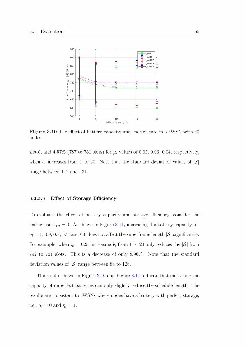
3.3. Evaluation 56
1 5 10 15 20
550
600
650
700
750
800
850
900
950
=0
=0.01
=0.02
=0.03
=0.04
Figure 3.10 The effect of battery capacity and leakage rate in a rWSN with 40nodes.
slots), and 4.57% (787 to 751 slots) for µi values of 0.02, 0.03, 0.04, respectively,
when bi increases from 1 to 20. Note that the standard deviation values of |S|
range between 117 and 131.
3.3.3.3 Effect of Storage Efficiency
To evaluate the effect of battery capacity and storage efficiency, consider the
leakage rate µi = 0. As shown in Figure 3.11, increasing the battery capacity for
ηi = 1, 0.9, 0.8, 0.7, and 0.6 does not affect the superframe length |S| significantly.
For example, when ηi = 0.9, increasing bi from 1 to 20 only reduces the |S| from
792 to 721 slots. This is a decrease of only 8.96%. Note that the standard
deviation values of |S| range between 84 to 126.
The results shown in Figure 3.10 and Figure 3.11 indicate that increasing the
capacity of imperfect batteries can only slightly reduce the schedule length. The
results are consistent to rWSNs where nodes have a battery with perfect storage,
i.e., µi = 0 and ηi = 1.

57 3.3. Evaluation
1 5 10 15 20
500
600
700
800
900
1000
1100
=1
=0.9
=0.8
=0.7
=0.6
Figure 3.11 The effect of battery capacity and storage efficiency in a networkwith 40 nodes.
3.3.4 Effectiveness of LS-rWSN
To analyse the performance of LS-rWSN, Section 3.3.4.1 computes the ratio R1
≥ 1 between its generated |S| and the optimal bound as per Propositions 3.1,
3.2, and 3.3 for Line, BTree, and Grid, respectively, for nodes with a perfect
battery, i.e., η = 0 and µ = 1. Recall that the optimal |S| is 4wr, 6wr, and 8wr
for Line, BTree, and Grid, respectively. Note that when nodes have a perfect
battery, the value of ρ is equal to the nodes’ harvesting time r. Apart from these
networks, Section 3.3.4.2 computes R2 to further evaluate LS-rWSN on arbitrary
networks, where R2 is the ratio between its generated |S| and the lower bound
|SE | in Eq. (3.1). For both types of networks, we set wi,j = 3, bi = 3, and ri = 1,
5, 10, 15, and 20.
3.3.4.1 Fixed Topologies
This experiment considers rWSNs with nodes from 20 to 100, with an increment
of 10 for the Line, BTree, and Grid topologies. As shown in Figure 3.12, LS-
rWSN always produced the optimal superframe for Line for any values of ri. On

3.3. Evaluation 58
the other hand, for ri = 1, BTree and Grid produce R1 = 1.28 and R1 = 1.42,
respectively. However, LS-rWSN has better performance for larger values of ri.
Specifically, when ri ≥ 5, LS-rWSN has a performance ratio R1 of 1.04 and
1.02 for BTree and Grid, meaning the superframe length is only 4% and 2%,
respectively, away from the optimal value for rWSNs with 20 to 100 nodes.
Figure 3.12 The performance of LS-rWSN in fixed topologies with a variousnumber of nodes for µi = 0 and ηi = 1.
3.3.4.2 Arbitrary Networks
For each network, consider µi = 0.01, and ηi = 0.7. The average ratio R2 in
Figure 3.13 is obtained by averaging 100 random node deployments. As shown in
Figure 3.13, for a rWSN with 20 nodes and ri = 1, i.e., when nodes always have
energy, LS-rWSN achieves an average performance ratio R2 of 3.01. However,
when nodes have a lower energy harvesting constraint, i.e., ri > 1 the performance
of LS-rWSN improves significantly. Specifically, for ri ≥ 5 and |V | = 20, LS-
rWSN on average produces superframes with R2 = 1.07, i.e., only 7% longer
than the lower bound computed using Eq. (3.1). Figure 3.13 also shows that
except for ri = 1, increasing the network size does not reduce the performance

59 3.3. Evaluation
of LS-rWSN. Further, it shows that increasing the network size from 20 to 50
reduces the performance due to the high level of interference. The standard
deviation values of the performance ratio in Figure 3.13 range between 0.01 and
0.98.
20 30 40 50
0
1
2
3
4
5
6
r=1
r=5
r=10
r=15
r=20
Figure 3.13 The performance of LS-rWSN in arbitrary networks for µi = 0.01and ηi = 0.7.
20 30 40 50
0
20
40
60
80
100
120
140
160
180
r=10, = 0.01, =0.7
Figure 3.14 The running time of LS-rWSN in arbitrary networks for ri = 10,µi = 0.01, and ηi = 0.7.

3.4. Chapter Summary 60
3.3.5 Running Time
To measure the running time of LS-rWSN, this experiment considers rWSN with
20 to 50 nodes with ri = 10, µi = 0.01 and ηi = 0.7. Each node has battery
capacity bi = 3 and each link has weight wi,j = 3. Figure 3.14 shows that the
running time of LS-rWSN becomes longer when the number of nodes increases.
More specifically, the running time of LS-rWSN is 21.9 ms for |V | = 20, and
gradually increases to 143.3 ms when |V | reaches 50 nodes. This is because there
are more links when |V | increases. The running time is thus increasing, which is
consistent with Proposition 3.7. Note that there are on average 125 (from 104 to
152 links), 273 (from 236 to 312), 470 (from 420 to 556), and 758 (from 670 to
854) links when there are 20, 30, 40, and 50 nodes, respectively. The standard
deviation of the running time in Figure 3.14 ranges between 6.35 and 17.66.
3.4 Chapter Summary
This chapter addressed link scheduling in rWSNs. It considered the following
factors: (i) energy harvesting time of nodes, (ii) battery capacity, (iii) imperfect
battery storage, i.e., leakage and storage inefficiency, and (iv) activation frequen-
cies wi. It presented a novel problem called LSHUS that aimed to produce a
link schedule S with the minimum length subject using the HUS protocol. This
chapter formally showed that LSHUS is NP-Complete and presented analytical
results for the optimal length for three bipartite topologies: Line, BTree, and
Grid. A greedy algorithm, called LS-rWSN, was proposed to solve LSHUS. Ex-
tensive simulations showed that factors such as harvesting time, battery leakage,
and storage efficiency significantly affected the schedule length. These factors
increased the length by up to 63.21%. On the other hand, battery capacity is
an insignificant factor, i.e., increasing the schedule length no more than 6.5%.

61 3.4. Chapter Summary
LS-rWSN produced the optimal superframe length for Line, and up to 1.28 and
1.42 times longer superframe lengths as compared to the theoretical superframe
length bound for BTree and Grid, respectively, for ri > 1. In Chapters 4 and 5,
we investigate using a battery cycle constraint to overcome the memory effect of
batteries.


Chapter 4
Link Scheduling in rWSNs with
Battery Memory Effect
This chapter considers the novel problem of deriving a TDMA link schedule for
rWSNs. Unlike past works, it considers: (i) the energy harvesting time of nodes,
(ii) Harvest-Store-Use (HSU) energy harvesting and battery usage protocol, (iii)
battery imperfections, and (iv) a battery cycle constraint that is used to overcome
the memory effect. Recall that such effect will reduce the battery’s usable capacity
if it is charged and discharged repeatedly after a partial discharge and charge,
respectively. This chapter shows analytically that the battery cycle constraint and
leaky batteries lead to unscheduled links. Further, it presents a greedy heuristic
that schedules links according to when their corresponding nodes have sufficient
energy.
This chapter considers a novel research aim: deriving a short TDMA link
schedule that considers nodes with a varying energy harvesting rate and battery
memory effect. To achieve this aim, solutions must address a number of problems.
Consider Figures 4.1a, 4.1b, and 4.1c. Note that links (v1, v2), (v1, v3), and (v1,
v4) interfere with each other and thus cannot be scheduled concurrently. Consider
63

64
the HSU battery usage protocol [32], where the harvested energy in slot t can
only be used in slot t + 1, t + 2, . . . . Node v1 needs to wait for three timeslots
to accumulate one unit of energy, denoted as v1|3, and this energy can only
be used after slot t = 3. First, consider the case where nodes have unlimited
battery capacity; denoted by ∼ in Figure 4.1a. Node v1 can use its stored energy
in timeslot t = 4. However, none of its links can be scheduled at time t = 4
because its neighbours have insufficient energy to receive a packet. For example,
link (v1, v2) can be scheduled no earlier than at slot 6 + 1 = 7. After node v1
transmits a packet to node v2 at time t = 7, its remaining energy is sufficient to
transmit a packet to node v3. Thus, link (v1, v3) is scheduled at time t = 8. Then,
node v1 needs to accumulate energy before it can transmit a packet to node v4.
Thus, link (v1, v4) is scheduled at slot t = 8 + 3 + 1 = 12, producing the schedule
length of 12.
v1 | 3
~
~
~
~v2 | 6 v3 | 7
v4 | 8
7 8
12
(a)
v1 | 3
1
1
1
1
v2 | 6 v3 | 7
v4 | 8
7 11
15
(b)
v1 | 3
3
2
2
2
v2 | 6 v3 | 7
v4 | 8
13 15
17
(c)
Figure 4.1 An example (a) with interference and harvesting time, (b) plusbattery capacity, and (c) plus battery cycle constraints. The number inside eachnode shows the capacity of its battery. The number next to each link denotes itsactivation time, and vx|z represents node x requiring z time slots to accumulateone unit of energy.
Next, consider the case where each battery has a capacity of one unit; see
Figure 4.1b. This means the battery at node v1 can be recharged only after it is
used at time t = 7. Thus, node v1 can transmit the second packet no earlier than
at time t = 7 + 3 + 1 = 11, i.e., after it has harvested sufficient energy. Further,

65 4.1. Preliminaries
it can transmit the third packet no earlier than time t = 11 + 4 = 15. Hence, the
schedule length is 15.
Lastly, consider the case where each battery has a battery cycle constraint;
see Figure 4.1c. Node v1 has a battery with three units of energy and nodes v2,
v3, and v4 each have a battery with two units of capacity. Thus, v1 needs to wait
until slot t = 3×3+1 = 10 to fully recharge its battery before it can transmit one
packet. However, it cannot do so because its neighbours’ battery is yet to be fully
recharged. That is nodes v2, v3, and v4 have to wait until slot t = 6× 2 + 1 = 13,
t = 15, and t = 17, respectively, before their battery can be discharged. The
schedule length in this case is 17.
The preliminary version of the work in this chapter has been presented in [92],
while its full version has been published in [93]. More specifically, reference [92]
described the problem and its solution for perfect batteries, while reference [93]
included imperfect batteries.
The layout of this chapter is as follows. Section 4.1 shows our network model
and formulates the problem. Section 4.2 consists of four subsections; it addresses
key properties of our proposed algorithm in Section 4.2.1, the feasibility study in
Section 4.2.2, a proposed method to shorten superframe length in Section 4.2.3,
and a proposed algorithm in Section 4.2.4. Section 4.3 provides simulation results
to show the performance of our approaches. Finally, Section 4.4 concludes the
chapter.
4.1 Preliminaries
Section 4.1.1 formalises our rWSN model and key notations used in this chapter.
After that, Section 4.1.2 formalises the problem of interest.

4.1. Preliminaries 66
4.1.1 Network Model
A node vi is equipped with a harvester that scavenges energy from its environ-
ment, e.g., solar, and it is equipped with a rechargeable battery with capacity bi
(in unit of ε). It uses the HSU battery usage protocol [32], where the harvested
energy at timeslot t must first be stored before it is used in later slots. Recall that
it is possible to revise the HSU model to apply in the HUS model. Let ri ≥ 1 (in
slots) be the harvesting time or total number of slots that is required by a node
vi to accumulate 1ε of energy. Thus, the harvesting rate of a node is εri
per time
slot. Let 0 < ηi ≤ 1 be the storage efficiency and 0 ≤ µi < 1 be the battery’s
leakage factor (per time slot) of a node vi. This work omits the following cases.
First, when ηi = 0 and µi = 1, the battery of nodes cannot store any harvested
energy and retain its energy, respectively. Second, in each slot, the amount of
harvested energy must be larger than the battery leakage rate µi. Otherwise, any
harvested energy will be lost immediately due to battery leakage. In both cases,
nodes will have no energy to activate links.
All nodes have a minimum battery capacity, i.e., for a node vi, we have bi ≥ 1ε.
They have a single rechargeable battery with a battery cycle constraint [36]. This
constraint requires the battery of a node vi to be: (i) charged to its maximum
capacity bi,max before it can be used/discharged, for 2 ≤ bi,max ≤ bi, and (ii)
discharged to its minimum capacity, bi,min ≥ 1, before it can be charged. We
call (i) and (ii) respectively as the discharging and charging constraint. Conse-
quently, the battery at each node vi can be in one of two modes: (i) charging,
or (ii) discharging. More specifically, the battery cannot be in the charging and
discharging mode at the same time. Without loss of generality, we assume each
battery has an initial energy level of bi,min. Further, we assume bi,min and bi,max
are integers, where bi,min < bi,max.

67 4.1. Preliminaries
For a node vi, let t+i,k and t−i,k respectively, be the start and end time of its k-th
charging cycle. Similarly, for discharging cycle k at a node vi, its start and end
time are denoted respectively as t+i,k and t−i,k. Further, τi,k and τi,k respectively
are the charging and the discharging time intervals of the battery at a node vi in
cycle k ≥ 1; these quantities are computed as τi,k = t−i,k− t+i,k and τi,k = t−i,k− t
+i,k.
In other words, the battery at a node vi is being charged during time interval τi,k
and being discharged during time interval τi,k for each cycle k. As illustrated in
Figure 4.2, each battery follows a sequence of a charge-discharge cycle. Thus, we
have t+i,k = t−i,k + 1 and t+i,k = t−i,k + 1. Note that for each cycle k, the value of τi,k
is dependent on ri, ηi as well as bi,max, while the length of τi,k is affected by bi,min
and the number of times the battery is used to transmit/receive packets at each
cycle k, denoted by ui,k. In addition, both times are affected by the battery’s
leakage factor µi. Note that as ri, µi, ηi, and bi,max are constants, all intervals
τi,k have equal length. In contrast, the value of τi,k may vary at different cycles
because ui,k varies according to the number of transmitted/received packets. In
the remainder of this chapter, the cycle number k is omitted if the context is
clear.
charging
cycle 1
discharging
cycle 1
charging
cycle 2
discharging
cycle 2
Figure 4.2 Charge-discharge cycles at a node vi at cycle k = 1 and k = 2.
Let bi,t and bi,t (in unit of ε) denote the energy level of the battery at a node
vi during a charging and discharging cycle at time slot t, respectively. Thus,
we have bi,t−i = bi,max and bi,t−i = bi,min. The battery level of a node vi at the
beginning of each charging cycle, i.e., at time t+i , is
bi,t+i = bi,min − µibi,min = (1− µi)bi,min. (4.1)
4.1. Preliminaries 68
This is because: (i) the battery stops discharging at time t−i = t+i − 1 when the
amount of energy reaches bi,min, and (ii) there is energy leakage of µibi,min from
time t+i − 1 to t+i . On the other hand, the battery level of a node vi at the start
of discharging cycle t+i is
bi,t+i = bi,max − µibi,max = (1− µi)bi,max (4.2)
This is because: (i) the battery stops charging at time t−i = t+i − 1 when its
battery level reaches its maximum capacity, i.e., bi,max, and (ii) there is energy
leakage of µibi,max from time t+i − 1 to t+i .
Let Ti be the earliest time slot when the battery at a node vi is in discharging
mode. The earliest time in which a link li,j can be scheduled is at time ti,j =
max(Ti, Tj), i.e., when the end nodes of a link li,j can discharge their battery.
For each node vi, we initialise Ti to τi + 1. It is updated when the battery at a
node vi is discharged to transmit/receive a packet.
Figure 4.3a presents a rWSN with four nodes to illustrate our network model.
It shows values of bi,min, bi,max, bi, µi, ηi, and ri for each node vi as well as
the weight of each link li,j. The battery level of each node vi in charging and
discharging mode is computed using Eq. (4.1) and (4.2), e.g., b1,t+1 = b1,max×µ1 =
5× 0.99 = 4.95 and b1,t+1 = b1,min × µ1 = 1× 0.99 = 0.99, respectively. As shown
later in Section 4.2, one can compute the charging time and discharging time
intervals for each battery to obtain τ1 = 9, τ2 = 12, τ3 = 20, and τ4 = 10. Thus,
we have T1 = τ1 + 1 = 10, T2 = 13, T3 = 21, and T4 = 11. Therefore, the earliest
time each link li,j can be scheduled is computed as t1,2 = max(10, 13) = 13,
t2,4 = 13, and t3,1 = 21. In Figure 4.3b, there are two links that experience
primary interference, namely, link l3,1 with l1,2 and l1,2 with l2,4. Also shown is
secondary interference at node v1 that is caused by node v2, i.e., link l3,1 with l2,4.

69 4.1. Preliminaries
v1 | 2
v3 | 8
v2 | 5
v4 | 3
b1 = 5
b3 = 3
b2 = 3
b4 = 4
w3,1 = 1 w2,4 = 3
w1,2 = 2
b1,min = 1
b1,max = 5
μ1 = 0.01
η1 = 1
b2,min = 1
b2,max = 3
μ2 = 0.01
η2 = 1
b3,min = 1
b3,max = 3
μ3 = 0.01
η3 = 1
b4,min = 1
b4,max = 4
μ4 = 0.01
η4 = 1
(a) (b)
Figure 4.3 A rWSN as a (a) graph G, and its (b) conflict graph CG.
4.1.2 Problem Statement
Given a rWSN, our problem, called Link Scheduling with Memory Effect-
1 (LSME-1), is to generate the TDMA link schedule S with minimum length
|S| that satisfies the following constraints: (i) the battery at each node vi ∈ V
satisfies the battery cycle constraint, (ii) each link li,j ∈ E can be scheduled at
timeslot t only if its end nodes are in discharging mode, (iii) each link li,j ∈ E is
scheduled at least wi,j times in S.
Figure 4.4 shows two example of link schedules. Figure 4.4a presents a fea-
sible link schedule with 320 slots which satisfies constraints (i), (ii), and (iii).
Figure 4.4b gives a shorter feasible schedule with |S| = 307 slots. Note that link
scheduling is known to be NP-hard; works such as [59] and [43] assumed nodes
with unlimited energy. This is simply a special case of LSME-1. Thus, our
problem is also NP-hard.
Slot: 1 … 20 … 30 … 140 … 160 … 230 … 320
Schedule: l2,4 l3,1 l2,4 l1,2 l1,2 l2,4
(a) One feasible TDMA link schedule.
Slot: 1 … 13 … 21 … 128 … 152 … 227 … 307
Schedule: l2,4 l3,1 l2,4 l1,2 l1,2 l2,4
(b) The optimal TDMA link schedule.
Figure 4.4 TDMA link schedules for the rWSN in Figure 4.3 with a batterycycle constraint. Gray coloured slots show no transmissions/receptions. Notethat the figure shows only non-empty slots with empty slot represented as “. . . ”.

4.1. Preliminaries 70
4.1.3 Problem Analysis
We now analyse the effect of a battery cycle constraint on the schedule length
for three fixed topologies, i.e., Line, Binary Tree (BTree), and Grid ; see Sec-
tion 2.6.1.1 for their detailed configurations. We consider that each node has
equal harvesting time of r > 0, that a battery’s usable energy b ≥ 1, and the link
weight w ≥ 1. Note that b is equal to bmax−bmin. The following Propositions 4.1,
4.2, and 4.3 show the effect of a battery cycle constraint on the schedule length
for Line, BTree, and Grid, respectively.
Proposition 4.1. The optimal link schedule for a Line topology with n ≥ 3 has
superframe length
|S| =⌈
4w
b
⌉× rb+ 4w (4.3)
Proof. We first describe by construction how to derive a link schedule for Line
when each node always has energy to transmit/receive packets. For this case with
w = 1, we can schedule links in four different slots as follows. Links in the set
{(2+4i, 3+4i), (5+4i, 4+4i)} can be scheduled in a slot A, for i = 0, 1, · · · , b(n−
2) / 4c; e.g., for n = 9, slot A contains links {(2, 3), (5, 4), (6, 7), (9, 8)}. Then,
reverse the direction of each link in slot A, and schedule the reversed link in slot
B; e.g., slot B contains links {(3, 2), (4, 5), (7, 6), (8, 9)}. Next, schedule links in
the set {(1 + 4i, 2 + 4i), (4 + 4i, 3 + 4i)} in slot C for i = 0, 1, · · · , b(n− 2) / 4c;
e.g., links {(1, 2), (4, 3), (5, 6), (8, 7)}. Finally reverse the links in slot C for slot
D; e.g., links {(2, 1), (3, 4), (6, 5), (7, 8)}. For w > 1, repeat the described four-
slot link schedule, in the same order, for w − 1 times. Thus, we have |S| = 4w.
For example, for w = 2, the following sequence of 4× 2 = 8 slots are constructed:
S = (A,B,C,D,A,B,C,D).
Next, consider the case where each battery follows the battery cycle con-
straint. Notice that each node requires r × b slots to charge its battery to the

71 4.1. Preliminaries
maximum level before it can be used to transmit/receive b packets with no ad-
ditional charging. In other words, there are r × b empty slots, at which time
each node charges its battery to the maximum level, before the battery can be
used to activate, at most, b number of links. Thus, in general, there are in total
4w non-empty slots where links are activated, and⌈4w
b
⌉× rb empty slots where
batteries are being charged. For example, consider r = 2, and b = 3 for the afore-
mentioned eight slot schedules S. Due to the battery cycle constraint, there are
2× 3 = 6 empty slots before links in slot A can be activated at Slot-7. Links in
slot B and C are activated at Slot-8 and Slot-9, respectively. Then, nodes need to
recharge their battery to the maximum level, i.e., there are other 2×3 = 6 empty
slots, before links in slots D, A, and B can be activated at Slot-16, Slot-17, and
Slot-18, respectively. Finally, following the other six empty slots, links in slot C
and D are activated at Slot-25 and Slot-26, respectively. Thus, for this example,
|S| =⌈4×23
⌉× 2× 3 + 4× 2 = 26. The schedule length is optimal for the follow-
ing two reasons. Firstly, for n ≥ 3, some nodes in Line have four bidirectional
links. Thus, the schedule must contain at least 4w non-empty slots. Secondly,
each node needs rb empty slots before it can schedule b links. In other words,
there are at least⌈4w
b
⌉× rb number of empty slots. Thus, the schedule length of⌈
4w
b
⌉× rb+ 4w slots, shown in Eq. (4.3), is optimal.
Proposition 4.2. The optimal link schedule for a BTree with L ≥ 3 levels has
superframe length
|S| =⌈
6w
b
⌉× rb+ 6w (4.4)
Proof. We first outline the steps to construct a link schedule for a BTree when
each of its nodes always have energy. Links in a BTree with three levels can
be scheduled in six slots: Slot-1 = {(1, 2), (3, 6)}, Slot-2 = {(2, 1), (6, 3)}, Slot-3
= {(1, 3), (2, 4)}, Slot-4 = {(3, 1), (4, 2)}, Slot-5 = {(2, 5), (3, 7)}, and Slot-6 =

4.1. Preliminaries 72
{(5, 2), (7, 3)}. The link schedules for a four-level BTree can be generated from
the schedules of two BTree with three levels as follows. Denote the larger tree
as T with root R, and the two smaller trees as T1 and T2 with root R1 and
R2, respectively. Tree T is constructed from T1 and T2 by connecting R to R1
with two bidirectional links, and R to R2 with two other links, i.e., T1 and T2
are the left and right subtrees of T , respectively. Thus, renumbering the nodes
in T , the label of nodes R, R1, and R2 are 1, 2, and 3, respectively. Links in
T are scheduled as follows. First, combine the links of T1 scheduled in one slot
with the corresponding links of T2 that are scheduled in the same slot number.
Notice that no links in T1 interfere with any links in T2, and vice versa. Then,
insert each of the four incident links at R into a slot that does not contain any
link that interferes with it. More specifically, links (1, 2), (2, 1), (1, 3), and (3, 1)
are inserted into a slot that contains links (8, 4), (4, 8), (12, 24), and (24, 12),
respectively. Using the same steps, one can schedule links in a five-level tree
using the six-slot schedules of its two four-level subtrees. Repeating the process,
one can always generate the link schedules of a tree with k levels in six slots from
the schedules of its two subtrees with (k − 1) levels, for any k ≥ 4. For w > 1,
repeat the described six-slot link schedule in the same order for w − 1 times.
Thus, we have |S| = 6w.
Next, consider the case where each battery follows the battery cycle con-
straint. Notice that each node requires r × b slots to charge its battery to the
maximum level before it can be used to transmit/receive b packets with no ad-
ditional charging. In other words, there are r × b empty slots, at which time
each node charges its battery to the maximum level, before the battery can be
used to activate, at most, b number of links. Thus, in general, there are in total
6w non-empty slots where links are activated, and⌈6w
b
⌉× rb empty slots where
batteries are being charged.

73 4.1. Preliminaries
The schedule length is optimal for the following two reasons. Firstly, for
L ≥ 3, some nodes in a BTree have six bidirectional links. Thus, the schedule
must contain at least 6w non-empty slots. Secondly, each node needs rb empty
slots before it can schedule b links. In other words, there are at least⌈6w
b
⌉× rb
number of empty slots. Thus, the schedule length of⌈6w
b
⌉× rb+ 6w slots, shown
in Eq. (4.4), is optimal.
Proposition 4.3. The optimal link schedule length for a Grid of size row ≥ 3
and col ≥ 3 is
|S| =⌈
8w
b
⌉× rb+ 8w (4.5)
Proof. We first outline the steps to construct a link schedule for a Grid when
each of its nodes always has energy. From Proposition 4.1, the link schedule of
each Line graph requires 4w non-empty slots. Next, the following describes how
to produce the schedule for a Grid with length 8w. Further, the length is shown
to be optimal.
Consider the schedule of links in row Line graphs. One can observe that links
in odd rows can be activated in 4w slots. Similar rules apply for links in even rows.
Further, except for links in two consecutive rows, there is no other interference.
Without loss of generality, consider links in R2 and R3 in Figure 2.4. Note that
there is an interference only between nodes in each (2×2) Grid, e.g., nodes {4, 5}
at R2 and {7, 8} at R3, and when their links are in opposite directions, e.g.,
links (4, 5) and (8, 7) that incur interference at nodes 5 and 7. To prevent any
interference, each slot must contain links of the same directions, e.g., links (4, 5)
and (7, 8). Thus, links in all rows can be scheduled in 4w slots. As an example, for
Figure 2.4 with w = 1, the four slots are: Slot-1 = {(1, 2), (4, 5), (7, 8), (10, 11)},
Slot-2 = {(2, 1), (5, 4), (8, 7), (11, 10)}, Slot-3 = {(2, 3), (4, 5), (8, 9), (11, 12)},
and Slot-4 = {(3, 2), (6, 5), (9, 8), (12, 11)}. Use the same construction for links

4.2. Solution 74
in all columns. More specifically, these links are scheduled in 4w slots. Thus, all
links in a Grid can be scheduled in 4w + 4w = 8w slots. Next, consider the case
where each battery follows the battery cycle constraint. Notice that each node
requires r × b slots to charge its battery to the maximum level before it can be
used to transmit/receive b packets with no additional charging. In other words,
there are r × b empty slots, at which time each node charges its battery to the
maximum level, before the battery can be used to activate at most b number of
links. Thus, in general, there are in total 8w non-empty slots where links are
activated, and⌈8w
b
⌉× rb empty slots where batteries are being charged.
The schedule length is optimal for the following two reasons. First, for row ≥ 3
and col ≥ 3, some nodes in (row × col) Grid have eight bidirectional links, e.g.,
node 5 and 8 in Figure 2.4. Thus, the link schedule of a Grid requires at least 8w
non-empty slots. Secondly, each node needs rb empty slots before it can schedule
b links. In other words, there are at least⌈8w
b
⌉× rb number of empty slots. Thus,
the schedule length of⌈8w
b
⌉× rb+ 8w slots shown in Eq. (4.5) is optimal.
4.2 Solution
This section first describes eight propositions relied upon by our greedy algorithm.
It then provides two propositions to show that LSME-1 might not have a feasible
solution when the battery of each node has a non-negative leakage rate, i.e.,
µi > 0. Finally, the details of the proposed greedy algorithm are presented in
Section 4.2.4.
4.2.1 Key Properties
Propositions 4.4 and 4.5 relate to batteries in a charging cycle, and Proposi-
tions 4.6 to 4.11 relate to batteries in a discharging cycle. For brevity, we define

75 4.2. Solution
ri = ri/ηi, and µi = 1− µi.
Proposition 4.4. The energy level (in ε) of a battery in the charging mode at a
node vi at time slot t, for t+i ≤ t ≤ t−i , is
bi,t = min
bi,max, bi,min × µit−t+i +1 +
t−t+i −1∑p=0
µip
ri
(4.6)
Proof. The stored energy at time t+i + 1 is computed by subtracting the energy
lost due to battery leakage, i.e., µibi,t+i plus the energy harvested at slot t+i , i.e.,
1/ri. Thus, bi,t+i +1 = (1−µi)bi,t+i +1/ri. The energy level bi,t+i +2 is computed from
bi,t+i +1 by (i) subtracting the energy leakage that occurs from time t+i +1 to t+i +2,
(ii) adding the energy harvested in time slot t+i + 1, and (iii) substituting bi,t+i +1
with (1− µi)bi,t+i + 1/ri. Steps (i) and (ii) obtain bi,t+i +2 = (1− µi)bi,t+i +1 + 1/ri.
Step (iii) substitutes bi,t+i +1 with (1 − µi)bi,t+i + 1/ri to produce bi,t+i +2 = (1 −
µi)[(1 − µi)bi,t+i ] + 1/ri = (1 − µi)2bi,t+i + (1 − µi)/ri + 1/ri. Then, using energy
level bi,t+i +2, steps (i) to (iii) are used to compute the energy level at time t+i + 3,
i.e., bi,t+i +3 = (1− µi)3bi,t+i + (1− µi)2/ri + (1− µi)/ri + 1/ri. Repeating steps (i)
to (iii) for time t+i +4, . . . , t−1, t, we obtain the stored energy at the beginning of
time t, i.e., bi,t = (1−µi)t−t+i bi,t+i +
∑t−t+i −1p=0 (1−µi)p/ri. Substituting (1−µi)bi,min
in Eq. (4.1) for bi,t+i , we have bi,t = (1−µi)t−t+i +1bi,min+
∑t−t+i −1p=0
(1−µi)pri
. However,
bi,t is bounded by the upper limit of battery capacity bi,max, which implies bi,t ≤
bi,max. Substituting (1 − µi) with µi, we obtain the expression stated in the
proposition.
Note that when the battery has 100% storage efficiency and no leakage, i.e.,
ηi = 1 and µi = 0, respectively, Eq. (4.6) is reduced to
bi,t = min(bi,max, bi,min + (t− t+i )/ri) (4.7)

4.2. Solution 76
Proposition 4.5 computes the charging time interval τi = t−i − t+i of the battery
at a node vi, i.e., the number of slots needed to charge the battery to its maximum
level bi,max starting from its minimum level bi,min.
Proposition 4.5. The charging time interval for the battery of a node vi is
computed as
τi =
ri(bi,max − bi,min), ηi = 1 and µi = 0
dlog (
1−riµibi,max1−riµiµibi,min
)
log µie, 0 < ηi < 1 and 0 < µi < 1
(4.8)
Proof. We set t = t−i in Eq. (4.6) to compute the maximum energy level of the
battery at a node vi, i.e., bi,max. Thus, we have
bi,max = bi,min × µiτi+1 +
τi−1∑p=0
µip
ri(4.9)
For case (i): ηi = 1 and µi = 0, we set µi = 1 and ri = ri in Eq. (4.9) to yield
bi,max = bi,min + τi/ri. Thus, τi = ri(bi,max − bi,min) as shown in Eq. (4.8). For
case (ii): 0 < ηi < 1 and 0 < µi < 1, i.e., µi 6= 1, we use the geometric series [94]
to produce∑τi−1
p=0µip
ri= 1
ri
µτii −1µi−1 . Thus, Eq. (4.9) becomes
bi,max = bi,min × µiτi+1 +1
ri
µτii − 1
µi − 1(4.10)
Solving Eq. (4.10) for τi, we obtain Eq. (4.8).
The amount of energy that leaks from the battery of a node vi per slot, i.e.,
riµi, and the battery’s leakage rate µi in case (ii) of Eq. (4.8), must be less than
1bi,max
and 1riµibi,min
, respectively. Otherwise, the battery will never be able to
charge to its maximum level.

77 4.2. Solution
We first present Eq. (4.11) and (4.12) that are used in Propositions 4.6 and
4.7. Consider a battery of a node vi with an energy level of x at time t1, i.e.,
bi,t1 = x. As the battery leaks, the energy level of the battery at time t2 ≥ t1 is
reduced to
bi,t2 = xµt2−t1i (4.11)
Eq. (4.11) is used to compute the amount of energy that has leaked from the
battery of a node vi from time t1 to t2, i.e., ∆t2i,t1
= bi,t1 − bi,t2 for bi,t1 = x as
∆t2i,t1
= x(1− µt2−t1i ) (4.12)
Propositions 4.6 to 4.11 relate to a battery in discharging mode. Propo-
sition 4.6 computes the energy level of the discharging battery at time t, for
ti < t ≤ t−i , where ti is the most recent time the battery was used. From time ti
to t, the energy level decreases due to battery leakage only. Thus, Proposition 4.6
is valid only for batteries with a non-negative leakage rate, i.e., µi > 0.
Proposition 4.6. The energy level (in ε) of the discharging battery at a node vi
at timeslot t, for ti < t ≤ t−i is
bi,t = max(bi,min, bi,max × µt−t+i +1i − µt−tii ) (4.13)
Proof. Following Eq. (4.2), the battery level at time t+i is bi,t+i = bi,max×µi. Using
Eq. (4.12), the amount of energy leaked from time t+i to ti, for x = bi,t+i is
∆tii,t+i
= bi,t+i × (1− µti−t+i
i ) (4.14)
Thus, after spending 1ε of energy at time ti, the remaining energy of the battery
at the end of slot ti is
bi,ti = bi,t+i −∆tii,t+i− 1 (4.15)

4.2. Solution 78
Now, as per Eq. (4.12), the energy leaked from time ti to t, for x = bi,ti , is
∆ti,ti
= bi,ti × (1− µt−tii ) (4.16)
Thus, the remaining energy at time t is
bi,t = bi,ti −∆ti,ti
(4.17)
Using (4.2) in (4.14), (4.2) and (4.14) in (4.16), (4.15) in (4.16), and (4.15) and
(4.16) in (4.17), we obtain
bi,t = bi,max × µt−t+i +1i − µt−tii (4.18)
As the energy level is lower bounded by bi,min, we thus obtain Eq. (4.13).
Note that when the leakage rate is µi = 0, the energy level of a battery at a
node vi at time slot t is bi,t = bi,ti − 1. This is because the energy level decreases
only due to packet transmission/reception.
Let δb2i,b1 be number of timeslots needed to discharge the battery of a node vi
from level b1 ≤ bi,max to b2 ≥ bi,min due to battery leakage only. The following
Proposition 4.7 computes δb2i,b1 , which is applicable only when each battery has a
non-negative leakage rate of µi > 0.
Proposition 4.7. The discharging time interval, due to battery leakage only, for
the battery of a node vi, to decrease from b1 ≤ bi,max to b2 ≥ bi,min is given as
δb2i,b1 = b log(b2)− log(b1)
log(µi)c (4.19)

79 4.2. Solution
Proof. First, we set ∆t2i,t1
= b1− b2 and x = b1 in Eq. (4.12). As a result, we have
b1 − b2 = b1(1− µδb2i,b1i ) (4.20)
Then we solve Eq. (4.20) for δb2i,b1 to obtain Eq. (4.19).
Proposition 4.8 computes the next earliest time when the battery at a node
vi can be used to transmit/receive a packet.
Proposition 4.8. Consider the battery at a node vi is last used at time ti ≥
τi + 1. The next earliest timeslot when the battery at a node vi can be used to
transmit/receive a packet is
Ti =
ti + σi,ti × τi + 1, µi = 0
ti + σi,ti × (δb2i,b1 + τi) + 1, µi > 0
(4.21)
Proof. The next earliest time the battery at a node vi can be used depends on
the remaining battery level at time ti, i.e., bi,ti . For Case (i): µi = 0, Eq. (4.21)
considers two sub-cases: (a) bi,ti = bi,min, and (b) bi,ti > bi,min. For sub-case
(a), the battery needs to be recharged. This sub-case requires a charging time
interval of τi, computed by Eq. (4.8). Thus, we have Ti = ti + τi + 1 because the
harvested energy needs to be stored first before it can be used. For this sub-case,
σi,ti in Eq. (4.21) is set to 1. For sub-case (b), the battery at node vi can still be
discharged to transmit/receive another packet at time t+ 1, i.e., Ti = ti + 1, and
thus σi,ti in Eq. (4.21) is set to 0.
For Case (ii): µi > 0, there are two sub-cases: (a) bi,ti < (bi,min + 1), and
(b) bi,ti ≥ (bi,min + 1). For sub-case (a), when the remaining energy is less
than (bi,min + 1), the battery needs to be recharged. However, the battery cycle
constraint requires the energy level of the battery to reach bi,min first before it can

4.2. Solution 80
be recharged. Using Eq. (4.19), it takes b log(bi,min)−log( bi,ti )log(µi)
c slots to discharge the
battery (due to leakage) from level bi,ti = b1 to bi,min = b2. Then, we use Eq. (4.8)
to compute the charging time interval, τi. Thus, we have Ti = ti + (δb2i,b1 + τi) + 1
because the harvested energy needs to be stored first before it can be used. For
this sub-case, we have σi,ti = 1. For sub-case (b), the battery at a node vi can
still be discharged to transmit/receive another packet at time ti. Thus, the next
earliest time the battery at a node vi can be discharged to transmit/receive a
packet is slot Ti = ti + 1. For this sub-case, we have σi,ti = 0.
For a given discharging cycle k, let Ti,k > Ti be the time at which the energy
level at a node vi is bmin + 1. In other words, Ti,k is the latest time the battery
can be used in the discharging cycle k.
Proposition 4.9. The latest time the battery can be used for a given discharging
cycle k is
Ti,k = Ti + b log(bi,min + 1)− log(bi,Ti)
log(µi)c (4.22)
Proof. The energy level at time Ti is bi,Ti . The discharging time interval from level
bi,Ti to bi,min+1 can be computed using Eq. (4.19) for b1 = bi,Ti and b2 = bi,min+1.
Thus, time Ti,k can then be obtained by computing the sum of time Ti and the
discharging time, as given in Eq. (4.22).
For a given time Ti,k, Proposition 4.10 computes the earliest time Ti at which
the battery at a node vi can be used to transmit/receive a packet. In other words,
Ti = t+i,k+1. Figure 4.5 illustrates the relationship between times Ti,k and Ti of
Propositions 4.9 and 4.10, respectively.
Proposition 4.10. The earliest time Ti > Ti,k at which the battery at a node vi
can be used is
Ti = Ti,k + blog bi,min − log bi,Ti,k
log µic+ τi + 1 (4.23)

81 4.2. Solution
k k + 1
TiTi,k Ti =
Figure 4.5 An illustration for Propositions 4.9 and 4.10. The dashed (solid)lines represent charging (discharging) cycles.
Proof. At time Ti,k, a node vi’s energy level is bi,min + 1. We need to discharge
it first to energy level bi,min before it can be recharged. The discharging time is
computed using Eq. (4.19), for b1 = bi,Ti,k = bi,min + 1 and b2 = bi,min, shown as
the second term of the right hand side of Eq. (4.23). Then, we need to charge
the battery from bi,min to bi,max before it can be used. We use Eq. (4.8) to
compute the charging time interval, τi. After its fully charged, as per the HSU
model, the battery can be discharged in the next slot, which explains the +1 in
Eq. (4.23).
Let αi be the duration from time Ti,k to t+i,k+1, i.e., αi = t+i,k+1 − Ti,k; see
Figure 4.6. Recall that t+i,k is the starting time of a discharging cycle k of the
battery at a node vi at which time the battery has energy level bi,max × µi. The
time duration αi includes (i) time to discharge 1ε of energy, i.e., from bi,min + 1
to bi,min at cycle k, before the battery can start charging at cycle k + 1, (ii) time
to charge the battery from level bi,min to bi,max at cycle k+ 1, and (iii) a one slot
delay before the stored energy can be used at time t+i,k+1, as required by the HSU
model. One can use Eq. (4.19) with b1 = bi,min + 1 and b2 = bi,min to compute
(i), and Eq. (4.8) to compute (ii). Thus, we have
αi = b log(bi,min)− log(bi,min + 1)
log(µi)c+ τi + 1 (4.24)

4.2. Solution 82
Let βi denote time duration from t+i,k to Ti,k, i.e., βi = Ti,k−t+i,k; see Figure 4.6.
In other words, the battery takes βi slots to discharge all its stored energy (due
to leakage only) from level bi,t+i,k= bi,max × µi to bi,min + 1. Using Eq. (4.19), we
have
βi = b log (bi,min + 1)− log (bi,max × µi)log µi
c (4.25)
The following proposition computes t+i,k+m and Ti,k+m for the battery at a node
vi in a discharging cycle k +m, for integer m = 0, 1, . . ..
Proposition 4.11. Consider the battery of a node vi in a discharging cycle k,
and the battery is not used from time t+i,k to Ti,k+m, for any integer m = 0, 1, . . ..
For a given Ti,k, the value of t+i,k+m and Ti,k+m can be computed as
t+i,k+m = Ti,k +mαi + (m− 1)βi (4.26)
Ti,k+m = Ti,k +mαi +mβi (4.27)
Proof. For m = 0, we have t+i,k = Ti,k−βi, which is true by definition. For m = 1,
we have t+i,k+1 = Ti,k + αi, which is also true by the definition of αi or Eq. (4.24).
To compute t+i,k+2, we must include the number of slots required to discharge
the battery from the energy level at time t+i,k+1 to that at time Ti,k+1, and the
time duration from time Ti,k+1 to time t+i,k+2. Thus, t+i,k+2 = Ti,k+1 + αi + βi =
Ti,k + 2αi + βi. Similarly, for m = 3, we have t+i,k+3 = Ti,k+2 + αi + βi = Ti,k +
3αi+2βi. Repeating the steps to compute t+i,k and Ti,k for m = 4, 5, . . ., we obtain
Eq. (4.26) and Eq. (4.27), respectively. Note that for each pair of Ti,k and t+i,k at
any discharging cycle k, we have βi = Ti,k − t+i,k.
Figure 4.6 illustrates the relationship between αi, βi, t+i,k, and Ti,k used in
Eq. (4.24), (4.25), (4.26), and (4.27), respectively. Note that variable Ti,k is used

83 4.2. Solution
Ti,k Ti,k+1 Ti,k+mTi,k+m-1
k k + 1
�i �i �i
... k + m
�i �i
Figure 4.6 An illustration for Eq. (4.24) to Eq. (4.27).
only for batteries with a leakage rate of µi > 0. Thus, Propositions 4.9, 4.10, and
4.11 are not relevant for batteries with a leakage rate of µi = 0.
We now describe a scenario to schedule a link li,j in Figure 4.7. Consider a link
li,j and case (i): t+i,k < t+j,k in Figure 4.7a. A link li,j can be activated at timeslot
ti,j = max{t+i,k, t+j,k} = t+j,k only if (a) ti,j ≥ t+j,k+n, and (b) t+j,k+n ≤ Ti,k+m, for
m,n = 0, 1, . . .. Similarly, for case (ii): t+j,k < t+i,k in Figure 4.7b, a link li,j can
be activated at timeslot ti,j = t+i,k only if (a) ti,j ≥ t+i,k+m, and (b) t+i,k+m ≤ Tj,k+n.
In other words, we need to compute the two inequalities: (i) t+j,k+n ≤ Ti,k+m and
(ii) t+i,k+m ≤ Tj,k+n to determine the time ti,j to schedule each link li,j. Using
Eq. (4.26) and (4.27), for inequalities (i) and (ii), we obtain, respectively,
n(αj + βj)−m(αi + βi) ≤ Ti,k − Tj,k + βj (4.28)
m(αi + βi)− n(αj + βj) ≤ Tj,k − Ti,k + βi (4.29)
...
...
Ti,k
Tj,k
infeasible
schedule
Ti,k+m
Tj,k+n
feasible
schedule
(a) Case (i): t+i,k < t+j,k.
...
...
Ti,k
Tj,k
Ti,k+m
Tj,k+n
(b) Case (ii): t+j,k < t+i,k.
Figure 4.7 Two scenarios to schedule a link li,j.
One can use Satisfiability Modulo Theories (SMT) solver, e.g., Mistral [95],
to solve linear inequalities over integers for expressions (4.28) and (4.29). The

4.2. Solution 84
Mistral solver implements the Cuts-from-Proofs algorithm [96]. The solver is able
to generate solutions for systems of linear inequalities that contain between 10
and 45 variables and between 15 and 50 inequalities per system. For problem
LSME-1, it is preferable to find a pair (m,n) with the minimum of max{m,n}
for inequalities (4.28) and (4.29) to minimise time ti,j so that a link (i, j) can
be scheduled earlier. Therefore, in this paper, we propose a simple heuristic
function, called findmn(.), to obtain such a pair of (m,n) for inequalities (4.28)
and (4.29). Function findmn (i, j, Ti,k, Tj,k) generates the values of m and n for
inequalities (4.28) and (4.29) as follows. Initially, it sets (m,n) = (0, 0). From
Eq. (4.26) and (4.27), increasing the value of m results in a larger t+i,k+m and Ti,k+m
value. Similarly, a larger n value increases t+j,k+n and Tj,k+n. To minimise time
ti,j, findmn(.) needs to find the minimum integer values for m and n. Consider
t+i,k < t+j,k, i.e., case (i) in Figure 4.7a, and t+j,k+n > Ti,k+m. For this case, a
larger value of Ti,k+m is needed. Thus, findmn(.) increases the value of m in
(4.28) from m = 0 to m′ = 1 to increase the value of Ti,k+m, which also increases
t+i,k+m. The function findmn(.) also finds the value of n′ from (4.28) when it
uses m′ = 1. Next it produces a new value of m in (4.29) using n′, e.g., m′′. If
m′′ ≤ m′, the values (m′ = 1, n′) satisfy both (4.28) and (4.29), thus it returns
(m′, n′). However, if m′′ > m′, it uses m′′ in (4.28) to further increase the value
of Ti,k+m and obtains a new value for n, e.g., n′′. If n′′ ≤ n′, it stops at a feasible
solution (m′′, n′). However, if n′′ > n′, it uses n′′ in (4.29) to generate an updated
value of m, e.g., m′′′, which is then used to obtain another new value for n in
(4.28), namely n′′′. Function findmn(.) repeats the iterations until it finds the
first feasible solution for m and n. Thus, the link (i, j) can be scheduled at time
ti,j = max(t+i,k+m, t+j,k+n).
To illustrate how the function findmn(.) works, consider a link li,j with Ti =
22, Ti,k = 74, Tj = 93, Tj,k = 132, αi = 78, αj = 81, βi = 90, and βj = 39. In

85 4.2. Solution
this example, Tj = t+j,k because t+j,k = Tj,k − βj = 132 − 39 = 93. However, we
have Ti 6= t+i,k, in which the battery at node vi has been used in a discharging
cycle k. From (4.28) and (4.29), we respectively have (i) 120n − 168m ≤ −19,
and (ii) 168m− 120n ≤ 148. Notice that the link li,j cannot be activated at time
ti,j = max(22, 93) = 93 because t+j,k > Ti,k; see Figure 4.8. Thus, we need to shift
the discharging cycle of the battery at node vi to the next cycle by increasing time
Ti,k+m. To shift one cycle, function findmn(.) sets m = m′ = 1 in (i) and obtains
n′ = 0. As shown in Figure 4.8, the cycle now starts at t+i,k+1 = 152 and ends
at Ti,k+1 = 242, which are obtained by substituting m = 1 into Eq. (4.26) and
(4.27), respectively. The function then sets m = m′ = 1 in (ii) and gets n′ = 1 > 0
that indicates the need for shifting the cycle for the battery at node vj by one
cycle. Otherwise, the link cannot be activated at time ti,j = max(152, 93) = 152
because t+i,k+1 > Tj,k; see Figure 4.8. Setting n = n′ = 1 in (4.29), the function
gets a new value of m, i.e., m′′ = 1. Notice that m′′ ≤ m′, indicating that we
do not need to further shift the duration for node vi, i.e., (m = 1, n = 1) is a
feasible solution for (4.28) and (4.29). Thus, the link li,j can be scheduled at time
ti,j = max(t+i,k+1, t+j,k+1) = max(152, 213) = 213.
22 74
93 132
m = 0
n = 0
152 242
m = 1
213 252
n = 1
Ti,kTiTi,k+1
Tj,kTjTj,k+1
Figure 4.8 A discharging cycle of the battery at node vi (top) and vj (bottom).

4.2. Solution 86
4.2.2 Problem Solution Feasibility
This section aims to show the feasibility of LSME-1. While, in general, two
linear inequalities always have a solution, the values of m and n can be non-
integers [96]. One can use proof of unsatisfiability in [96] to determine if two
linear inequalities have no integer solution. Thus, LSME-1 for batteries with
a leakage rate of µi > 0 might not have a feasible solution, i.e., there can be
some links li,j ∈ E which cannot be scheduled. This is because a link (i, j) can
be scheduled only when the batteries at its end nodes are simultaneously in a
discharging cycle at the start of the same slot m or n, or different slots m and n.
Recall that expressions (4.28) and (4.29) are for case µi > 0.
Consider a link (i, j) and slot t at which time the batteries of end nodes vi
and vj are in a charging and discharging cycle, respectively. Thus, the link (i, j)
at time t cannot be scheduled. We call such a link (i, j) as an unscheduled link
or u-link at time t, denoted by (i, j)t, if its end nodes’ other adjacent links will
never be scheduled at or after time t. Let Et ⊆ E be a set of u-links at time
t. Intuitively, when the batteries of the end nodes of each u-link have the same
harvesting time, storage efficiency, leakage rate, and minimum and maximum
battery levels, the batteries will never reach a discharging cycle at the same time,
and thus the link cannot be scheduled. This is because the batteries will have the
same charging and discharging intervals. The intuition is one possible necessary
condition that prohibits expressions (4.28) and (4.29) having integers m and n as
their solution. It is stated and formally proved in the following proposition.
Proposition 4.12. Each u-link (i, j)t ∈ Et cannot be scheduled if all batteries
have the same values of harvesting time ri, storage efficiency ηi, leakage rate µi,
minimum battery level bi,min, and maximum battery level bi,max.

87 4.2. Solution
Proof. The proof considers three cases: (i) set Et contains only one u-link (i, j)t,
(ii) set Et contains more than one u-links where any pairs of them are not adjacent
to each other, and (iii) set Et contains more than one u-link where some pairs of
them are adjacent to each other. For case (i), we show that u-link (i, j)t cannot be
scheduled as follows. For ri = rj, µi = µj, ηi = ηj, bi,min = bj,min, bi,max = bj,max,
Eq. (4.8) obtains τi = τj. Thus, for τi = τj, bi,min = bj,max, and µi = µj, Eq. (4.24)
produces αi = αj. Similarly, Eq. (4.25) has βi = βj. Let α denote both αi and αj,
and β denote both βi and βj. Further we set T = Ti,k−Tj,k. Thus, we can convert
expressions (4.28) and (4.29) into the following two expressions, respectively,
n(α + β)−m(α + β) ≤ T + β (4.30)
m(α + β)− n(α + β) ≤ −T + β (4.31)
One necessary condition for (4.30) and (4.31) to have integer solution for m and
n is when m 6= n. Otherwise, the batteries at node vi and node vj cannot be
simultaneously in a discharging cycle because both batteries have the same afore-
mentioned parameters, and thus they have the same charging interval and the
same discharging interval. Now, we aim to show that any solution for expres-
sions (4.30) and (4.31) cannot have integer values of m and n. Without loss of
generality, consider Ti,k > Tj,k, and thus T > 0. Multiplying both sides of (4.30)
by −1, we have
m(α + β)− n(α + β) ≥ −T − β (4.32)
Thus, from (4.31) and (4.32), we have
− T − β ≤ m(α + β)− n(α + β) ≤ −T + β (4.33)

4.2. Solution 88
or
−(T + β)
(α + β)≤ m− n ≤ (−T + β)
(α + β)(4.34)
Notice that we have (−T +β) < (α+β) because T is a positive integer. Thus, we
have (−T +β)(α+β)
< 1. Further, −(T +β)(α+β)
has a negative value, or we have −(T +β)(α+β)
< 0.
Thus, we have
−(T + β)
(α + β)< 0 ≤ m− n < (−T + β)
(α + β)< 1 (4.35)
Since m 6= n, i.e., m− n 6= 0, we have
0 < m− n < 1 (4.36)
which means the value of m − n is a fraction. Thus, either variable m or n is a
fraction.
For case (ii), we repeat the proof for case (i) for each u-link (i, j)t ∈ Et.
Accordingly, none of the u-links in the set can be scheduled. Finally, for case
(iii), arbitrarily consider one u-link (i, j)t ∈ Et. Following the proof for case
(i), u-link (i, j)t cannot be scheduled. Next, consider an adjacent link of (i, j)t,
e.g., a u-link (i, k)t. We argue that (i, k)t cannot be scheduled because all of
its parameters are unchanged. Note that the expressions (4.30) and (4.31) of
u-link (i, k)t can have integer solutions m and n, and thus the link (i, j) can be
scheduled only if the batteries’ parameters, i.e., leakage rate µi, storage efficiency
ηi, minimum battery level bi,min, and maximum battery level bi,max, change.
To illustrate Proposition 4.12, consider the network in Figure 4.9 in which the
link (1, 2) is activated first at slot 13. We have T1 = T2 = 93, T1,k = T2,k = 132,
T3 = 13, and T3,k = 52. Further, Et = {(2, 3), (3, 1)}. We show that u-link
(2, 3)t cannot be scheduled as follows. Eq. (4.8) obtains τ2 = τ3 = 12, while
Eq. (4.24) and (4.25) produce α2 = α3 = α = 81 and β2 = β3 = β = 39,

89 4.2. Solution
respectively. Further, we have T = T2,k − T3,k = 132 − 52 = 80. Thus, we have
−119120
< 0 ≤ m− n ≤ − 41120
< 1 for (4.35), and 0 < m− n < 1 for (4.36), meaning
either value of m or n is a fraction. Thus, u-link (2, 3)t=93 cannot be scheduled
and the parameters for u-link (3, 1)t remain unchanged. Similarly, u-link (3, 1)t
cannot be scheduled because all of its parameters are the same as those of u-link
(2, 3)t.
While it is important to find all necessary conditions that prohibit expres-
sions (4.28) and (4.29) to have integer values of m and n for their solution,
unfortunately, we failed to generate the conditions due to the complexity of the
problem.
w1,2 = 1
v1
v2 v3
w2,3 = 1
w3,1 = 1
Figure 4.9 A cycle with three nodes: an example for a non-existing solution.Each node vi has bi,min = 1, bi,max = 3, bi = 3, µi = 0.01, ηi = 1, and ri = 5.
The following proposition formally shows that LSME-1 for batteries with
µi = 0 always has a feasible solution.
Proposition 4.13. LSME-1 for batteries with a leakage rate of µi = 0 will always
have a feasible solution, i.e., it is possible to activate each link li,j ∈ E.
Proof. For a leakage rate of µi = 0, the battery at a node vi makes a transition
from a discharging to a charging cycle only after its energy is used to activate
at least one incident link at a node vi. Consider a link li,j ∈ E. Without loss of
generality, assume the battery at a node vi has a longer discharging cycle than at
a node vj. In other words, the battery at a node vi is less frequently used than

4.2. Solution 90
the battery at node vj. For this case, the battery at a node vj will transition to a
charging cycle earlier than the battery at a node vi. Thus, the battery at a node
vi remains in a discharging cycle while the battery at a node vj is being recharged
to its maximum level. When the battery at a node vj is back to a discharging
cycle, the link li,j can be activated.
4.2.3 A Method to Shorten Superframe Length
The link schedule of a rWSN that complies with the battery cycle constraint will
become longer when the batteries of nodes have a smaller leakage rate µi. The
reason is as follows. Consider a battery of a node vi that has an energy level of
bi,min + x, for x < 1ε. The battery cycle constraint requires the energy level of
the battery to reach bi,min before it can be recharged. However, discharging the
non-usable energy from the battery takes longer when its leakage rate is smaller.
As an example, consider a battery with bi,min = 1 and x = 0.5. For a leakage rate
of µi = 0.01, b1 = 1.5, and b2 = 1, Eq. (4.19) produces 40 timeslots to discharge
the 0.5ε of energy. The discharging time will significantly increase to 405464 slots
when its leakage rate is µi = 10−6. The longer discharging time leads to a longer
schedule because the battery requires more time before it can be recharged to
bi,max so that it can be used to activate links.
To shorten the discharging time, we assume each node is able to discard or
flush its excess energy x at slot t in the next slot t + 1. One way for a node to
flush excess energy of size x is by using the energy to transmit a dummy packet
in a given slot. This protocol, henceforth called energy flush, is similar to that
assumed in [36]. Briefly, the work in [36] used two batteries, called primary and
secondary, which were in discharging and charging mode, respectively. When the
secondary battery was fully charged, it became the primary battery, while the
91 4.2. Solution
other became the secondary battery, i.e., it goes into charging mode, even when
its energy level had not reached the minimum, i.e., bi,min in our model.
The use of the energy flush protocol affects the computation of Eq. (4.19)
when it has b1 = bi,min + x for x < 1, and b2 = bi,min. For this case, the value of
δb2i,b1 is set to 1 because according to the energy flush protocol the x excess energy
can be discharged in one slot. Consequently, for this case, we need to set the
value of δb2i,b1 in Eq. (4.21) to 1. Thus, Eq. (4.21) for µi > 0, b1 = bi,min + x for
x < 1, and b2 = bi,min becomes
Ti = ti + σi,ti × (1 + τi) + 1 (4.37)
4.2.4 LSBCC
This section provides the details of our heuristic algorithm to solve LSME-1,
called Link Scheduler with Battery Cycle Constraint (LSBCC). The al-
gorithm aims to schedule all non-interfering links at the earliest possible timeslot
when the battery at its end nodes can be used, i.e., in discharging mode. Further,
it uses the conflict graph CG to check the interference links.
We first describe LSBCC in Algorithm 2 which considers batteries with a
leakage rate of µi > 0. LSBCC sets time t = 0 as the beginning of timeslot and
the battery of each node is initially in charging mode. In Lines 1−3, LSBCC uses
function INIT (.) to initialise the following eight parameters for each node vi. The
function initialises the energy level of the battery at each node vi to bi,min, i.e.,
bi,0 = bi,min. It uses Eq. (4.8) to compute τi, i.e., the charging time interval for the
battery at a node vi. It sets time duration αi and βi using Eq. (4.24) and (4.25),
respectively. It initialises ti to the last time the battery at a node vi is discharged
to zero. It also sets Ti to τi + 1 and Ti,k to Ti + βi. Recall that Ti and Ti,k are

4.2. Solution 92
the earliest time and the latest timeslot when the battery at a node vi can be
discharged to transmit/receive one packet. Finally, it initialises bi,Ti , the energy
level of the battery at a node vi at time Ti, to bi,max × µi, i.e., bi,Ti = bi,max × µi.
Algorithm 2 LSBCC
Input: G(V,E), ri, bi, bi,max, bi,min, µi, ηi of each node vi ∈ V , weight wi,j ofeach link li,j ∈ E, and conflict graph CGOutput: Superframe S1: for each node vi ∈ V do2: INIT (bi,0, τi, αi, βi, ti, Ti, Ti,k, bi,Ti)3: end for4: for each link li,j ∈ E do5: ti,j = COMP ti,j(vi, vj)6: end for7: K = {node li,j in CG with min{ti,j}}8: K ′ = ORDER(K)9: t←min{ti,j}
10: for each li,j ∈ K ′ do11: if NOT CONFLICT (li,j,S[t]) then12: S[t]← S[t] ∪ li,j13: wi,j ← wi,j − 114: if wi,j = 0 then15: remove node li,j from CG16: end if17: ti ← tj ← t18: bi,ti ← bi,Ti × µ
ti−Tii − 1
19: bj,tj ← bj,Tj × µti−Tjj − 1
20: Ti ← COMP Tα(i)21: bi,Ti ← COMP bα(i)22: Tj ← COMP Tα(j)23: bj,Tj ← COMP bα(j)
24: Ti,k ← Ti + b log (bi,min+1)−log bi,Tilog µi
c
25: Tj,k ← Tj + b log (bj,min+1)−log bj,Tjlog µj
c26: end if27: end for28: repeat Lines 4−27 until all wi,j = 0
Lines 4−6 use function COMP ti,j(.) in Algorithm 3 to compute the earliest
time each link (i, j) can be activated, i.e., ti,j. If the batteries of nodes vi and vj
are at the same discharging cycle, Line 2 of COMP ti,j(.) sets ti,j to the earliest

93 4.2. Solution
Algorithm 3 COMP ti,jInput: vi, vjOutput: ti,j
1: if Tj ≤ Ti,k or Ti ≤ Tj,k then2: ti,j ←max(Ti, Tj)3: else4: if SATISFY (i, j) is true then5: findmn(i, j, Ti,k, Tj,k)6: t+i,k+m ← Ti,k +mαi + (m− 1)βi7: t+j,k+n ← Tj,k + nαj + (n− 1)βj8: bi,t+i,k+m
← bi,max × µi9: bj,t+j,k+n
← bj,max × µj10: Ti,k+m ← Ti,k +mαi +mβi11: Tj,k+n ← Tj,k + nαi + nβi12: ti,j ←max(t+i,k+m, t
+j,k+n)
13: else14: ti,j ← 231 − 115: end if16: end if17: return(ti,j)
time at which both batteries can be discharged. On the other hand, when the two
batteries are not at the same discharging cycle, Lines 4−15 aim to obtain the
earliest time that the battery at nodes vi and vj can be at the same discharging
cycle. More specifically, Line 4 first uses the proof of unsatisfiability [96] in
function SATISFY (.) to determine if expressions (4.28) and (4.29) for a link (i, j)
have integer solutions. If so, Line 5 uses function findmn(.) to compute a pair
(m,n) that satisfies expressions (4.28) and (4.29). Otherwise, Line 14 sets ti,j to
a large integer value, i.e., 231−1, to denote that the link li,j can not be scheduled
in this iteration. Note that it is possible that the link li,j can be scheduled in the
future. Lines 6−7 compute the starting time of the next discharging cycle of the
battery at nodes vi and vj. Lines 8−9 obtain the battery levels of nodes vi and
vj. Lines 10−11 recompute the ending time of the next discharging cycle of the
battery at nodes vi and vj. Line 12 computes ti,j.

4.2. Solution 94
Line 7 of LSBCC creates a set K that stores all links (i, j) that have the same
earliest activation time. Line 8 then uses function ORDER(K) to sort links in
set K in order of decreasing weight wi,j. Links with equal wi,j are sorted in the
decreasing node degree of their end nodes, and for a tie, links are sorted in the
increasing order of their node labels.
Line 9 sets t with the earliest slot, i.e., min{ti,j}. Lines 10−27 repeatedly
schedule each link li,j ∈ K ′ in order. Each selected link in Line 12 does not
cause interference or is interfered by links that have been scheduled in slot t; see
the condition in Line 11. Each slot in S is initially empty. Note that function
CONFLICT (.) uses a matrix M of size |E|2 that contains Boolean variables to
represent the conflict graph of the network; i.e., M [a, b] is set to “1” if there is an
interference between links a and b. Line 13 decreases the weight of each selected
link li,j by one. Once the weight reaches zero (see Line 14 ), Line 15 removes the
link from contention.
Line 17 sets the last time that batteries at the end nodes of the selected link
li,j is used, i.e., ti and tj, to the current time. Further, Lines 18−19 compute
the energy levels of the battery at nodes vi and vj at time ti, after the nodes
have transmitted/received one packet. Line 20 uses function COMP Tα(.) that
implements Eq. (4.21) to update the next earliest time the battery at node vi
can be discharged. Line 21 uses function COMP bα(.) to compute the battery’s
energy level at time Ti, which depends on the remaining energy level at time ti,
i.e., bi,ti . More specifically, if bi,ti is greater than or equal to (bi,min + 1), then
bi,Ti is set to bi,ti × µi as the battery can still be used to transmit/receive one
packet. Otherwise, bi,Ti is set to bi,max× µi since the battery has been charged to
its maximum level. Similarly, LSBCC computes the next earliest time and energy
level of the battery at node vj in Lines 22−23. Lines 24−25 use Eq. (4.22) to
obtain the latest time the battery at nodes vi and vj can be used. Finally, the

95 4.2. Solution
steps from Line 4 are repeated until all links are scheduled, i.e., wi,j = 0.
Next, we describe how to adjust LSBCC in Algorithm 2 for use in the case
when the battery at each node vi is leak-free, i.e., for case µi = 0. The adjustment
comprises the following four changes to Algorithm 2: a) Function INIT (.) in
Line 2 of LSBCC does not initialise parameters αi, βi, and Ti,k. Recall that
these three parameters are used only for batteries with µi > 0; b) Replace Line
5 of Algorithm 2 with ti,j = max(Ti, Tj). Note that function COMP ti,j(.) is
applicable only for batteries with µi > 0; c) Set bi,Ti to bi,max in Line 21 if bi,ti is
equal to bi,min. Otherwise, set bi,Ti to bi,ti . Do a similar adjustment in Line 23 as
in Line 21 ; and lastly, d) Omit Lines 24−25.
For an example, consider the rWSN and conflict graph CG shown in Figure 4.3.
The function INIT (.) for each node vi sets the following eight parameters as: (i)
b1,0 = b2,0 = b3,0 = b4,0 = b1,min = 1; (ii) τ1 = 9, τ2 = 12, τ3 = 20, τ4 = 10;
(iii) α1 = 78, α2 = 81, α3 = 89, α4 = 79; (iv) β1 = 90, β2 = β3 = 39, β4 = 67;
(v) t1 = t2 = t3 = t4 = 0; (vi) T1 = τ1 + 1 = 10, T2 = 13, T3 = 21, T4 = 11;
(vii) T1,k = T1 + β1 = 100, T2,k = 52, T3,k = 60, T4,k = 78; and (viii) b1,T1 =
b1,max × µ1 = 5 × 0.99 = 4.95, b2,T2 = 2.97, b3,T3 = 2.97, b4,T4 = 3.96. Lines
4−6 obtain t1,2 = 13, t2,4 = 13, and t3,1 = 21. Line 7 inserts links l1,2 and l2,4
into the set K, and thus Line 8 obtains K ′ = {l2,4, l1,2} because w2,4 > w1,2, and
Line 9 sets t = 13. Line 11 finds that l2,4 has conflict with l1,2, and thus Line
12 inserts only link l2,4 into S[13], and Line 13 reduces w2,4 by one and hence it
becomes two. Line 17 sets t2 = t4 = 13. Lines 18−19 compute b2,13 = 1.97 and
b4,13 = 2.88. Lines 20−23 obtain T2 = 93, b2,T2 = 2.97 and T4 = 14, b4,T4 = 2.85.
Lines 24−25 then compute T2,k = 132 and T4,k = 49. Line 28 repeats the steps
from Line 4 until all links have wi,j = 0. Finally, LSBCC produces the link
schedule S in Figure 4.4b, i.e., S = [ S[13] = {l2,4}, S[21] = {l3,1}, S[128] =
{l2,4}, S[152] = {l2,4}, S[227] = {l1,2}, S[307] = {l1,2} ]. The generated schedule

4.3. Evaluation 96
contains 303 empty slots as the battery at each node needs time to charge to its
maximum level before it can be used to transmit/receive packets.
Proposition 4.14. The time complexity of LSBCC is O(W |E|2), where W =∑(i,j)∈|E|
(wi,j).
Proof. Lines 1−3 take O(|V |). Lines 4−6 require O(|E|) because Lines 1−17
of function COMP ti,j take O(1) each and these lines are repeated at most |E|
times. Line 7 takes O(|E|). Line 8 sorts all links in K using the function
ORDER(K) that requires O(|E| log |E|). Line 9 takes O(1). Line 11 requires
O(|E|2) to construct a matrixM which represents the conflict graph CG. Function
CONFLICT (li,j,S[t]) in Line 11 uses the matrix at most |E| times. Hence, it
takes O(|E|). Lines 12−25 take O(1) each. The for loop in Lines 10−27 is
repeated at most |E| times, and thus, the loop requires at most O(|E|2). Line 28
repeats Lines 4−27 W times. Thus, the time complexity of LSBCC is O(W |E|2).
Notice that the time complexity of LSBCC becomes O(|E|3) if each link weight
has a constant value. For this case, LSBCC runs in polynomial order of the
number of links |E|. Further, the running time of the algorithm worsens on the
networks that contain a high number of links. Nevertheless, since LSBCC runs
in polynomial order of |E|, it is scalable for use in larger sized networks.
4.3 Evaluation
Section 4.3.1 analyses the schedule length when nodes use a battery that adheres
to the battery cycle constraint but with no leakage. Section 4.3.2 aims to analyse
the effects of parameters ri, bi, bi,max, and ηi on the feasibility of LSME-1 when
nodes have a battery with a leakage rate of µi > 0. Finally, Section 4.3.3 evaluates

97 4.3. Evaluation
the impact of the battery cycle constraint on the link schedule length, and on
the number of charge/discharge cycles for rWSNs with leak-free batteries and for
those with batteries that leak.
Table 4.1 lists the parameter values used in our simulation. We consider
arbitrary networks with 10 to 50 nodes randomly deployed on a 40×40 m2 area.
The average number of links |E| are 28, 125, 273, 470, and 758 for networks
with 10, 20, 30, 40, and 50 nodes, respectively. Each node has a transmit and
interference range of 15 and 30 meters, respectively. We arbitrarily set the range
of values of ri and wi,j to {2, 3, . . . , 17} as in [44] and {1, 2, . . . , 5}, respectively.
We use leakage rate µi values in the set {1, 1.2, 1.4, 1.6, 1.8, 2.0, 2.2, 2.4}×10−6
per slot since the battery’s leakage rate is 20% per 24 hours [97]. We set each
slot to one second. Further, we consider batteries with 100% storage efficiency,
and arbitrarily set the values of bi, bi,min, and bi,max. Note that as reported in
Section 3.3.3.1 of Chapter 3, the battery capacity has an insignificant effect on
the superframe length |S|. Our results are an average of over 100 random node
deployments.
Table 4.1 Parameter values used in our evaluation.
Parameter Value (s)Network size 40×40 m2
Transmit range 15 mInterference range 30 m|V | {10, 20, 30, 40, 50}ri {2, 3, 4, . . . , 17}µi {1, 1.2, 1.4, 1.6, . . . , 2.4} × 10−6
ηi 1.0bi 3εbi,min 1εbi,max 3εwi,j {1, 2, 3, 4, 5}

4.3. Evaluation 98
4.3.1 Battery with No Leakage
The aim of this section is to study how the battery cycle constraint affects the
superframe length |S| when each battery has no leakage, i.e., µi = 0. Recall
that, as stated in Proposition 4.13, LSME-1 always has a feasible solution for
µi = 0. This section performs two evaluations. First, it compares the performance
of LSBCC against LSNBC. Briefly, LSNBC is a version of LSBCC without the
battery cycle constraint. Second, it investigates the effect of energy harvesting
time ri on the link schedules produced by LSBCC. All experiments consider 10 to
50 nodes with the following parameter values: bi = 3ε, bi,max = 3ε, and bi,min = 1ε.
4.3.1.1 LSBCC versus LSNBC
This section compares the performance of LSBCC against LSNBC in terms of
superframe length |S| and the total number of charge/discharge cycles. Briefly,
LSNBC is similar to LSBCC but without the battery cycle constraint. For this
experiment, we consider rWSNs with 10 to 50 nodes with harvesting time ri = 5.
We set the battery capacity bi to 3ε of energy, its minimum energy level bi,min to
1ε, and maximum energy level bi,max to 3ε. Each link weight is randomly fixed to
a value between 1 and 5, i.e., wi,j = [1, 5].
LSBCC vs LSNBC on Superframe Length: Figure 4.10 shows that the
superframe length |S| produced by LSBCC is longer than LSNBC. In a rWSN
with 10 nodes, LSBCC produces 42 more slots (30.43% longer) as compared to
using LSNBC. The results are consistent for other networks, i.e., |V | = 20, 30,
40, and 50 nodes. LSBCC produces superframes that are 19.4%, 17.9%, 17.94%,
and 17.47% longer than in LSNBC, respectively, with standard deviation values
ranging between 56 and 129. The reason for this is that nodes using LSBCC need
to wait for their batteries to be fully charged before they can discharge them.

99 4.3. Evaluation
10 20 30 40 50
0
200
400
600
800
1000
1200
LSNBC
LSBCC
Figure 4.10 LSBCC versus LSNBC in terms of |S|.
LSBCC vs LSNBC on Charge/Discharge Cycles: As shown in Fig-
ure 4.11, the number of charge/discharge cycles produced by LSBCC is less than
LSNBC. For example, when |V | = 10, LSBCC has 64 cycles less than in LSNBC;
i.e., 77.11% less. The results are consistent for |V | = 20, 30, 40, and 50. More
specifically, LSBCC requires 78.86%, 81.03%, 82.62%, and 84.05% fewer cycles
than LSNBC, respectively. This is because each battery in LSBCC needs to be
charged only when its energy level reaches the minimum. Notice that there is a
trade-off between longer link schedules and lesser charge/discharge cycles. For
example, for rWSN with |V | = 30, the number of cycles is reduced by 81.03%
at the expense of a 17.9% longer superframe length |S|. Recall that a battery
that has lower number of cycles will have a longer lifetime. In the remaining
experiments, we only consider LSBCC.
4.3.1.2 Effect of Harvesting Time
This section investigates the effect of harvesting time ri on |S| and charge/dis-
charge cycles. In this simulation, we consider various ri values, namely 1, 5, 10, 15,
and 20 slots, in a rWSN with 10 to 50 nodes. We set bi = 3ε, bi,min = 1ε,

4.3. Evaluation 100
10 20 30 40 50
0
500
1000
1500
2000
2500
3000
3500
4000
4500
LSNBC
LSBCC
Figure 4.11 LSBCC versus LSNBC on charge/discharge cycles.
bi,max = 3ε, and each link has weight wi,j = 3.
Effect on Superframe Length: From Figure 4.12, we see that the energy
harvesting time of nodes has a significant effect on |S|, i.e., increasing their energy
harvesting time results in a longer superframe. Specifically, for a rWSN with 10
nodes, when ri is increased by 4 slots, i.e., from 1 to 5, |S| jumps from 68 to
173 slots−an increase of 1.54 times. Similarly, when ri is increased from 5 to 20
with an interval of 5, i.e., from 5 to 10, 10 to 15, and 15 to 20, |S| is further
increased by 139, 140, and 140 slots, meaning the link schedule increases by 0.8,
0.45, and 0.31 times, respectively. We observe similar trends in rWSN with 20,
30, 40, and 50 nodes. For example, for a rWSN with 50 (100) nodes, when ri
increases from 1 to 20 with an interval of 5, |S| is increased by 1.33 (1.34), 0.72
(0.72), 0.42 (0.42), 0.3 (0.3) times, respectively. The increase in |S| is because
each battery needs more time to be charged to its maximum level before it can
be used to transmit/receive a packet. Also notice that the |S| for each network
size increases almost linearly when ri is increased from 1 to 20. Further, the rate
of increase (in slots) in smaller networks, e.g., |V | = 10, is less than that of larger
networks, e.g., |V | = 50. This is because more nodes mean that more links will
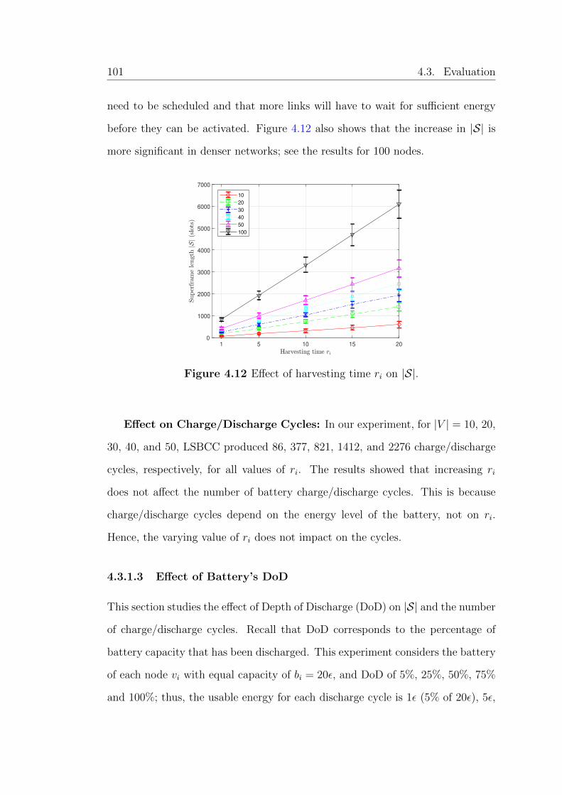
101 4.3. Evaluation
need to be scheduled and that more links will have to wait for sufficient energy
before they can be activated. Figure 4.12 also shows that the increase in |S| is
more significant in denser networks; see the results for 100 nodes.
1 5 10 15 20
0
1000
2000
3000
4000
5000
6000
7000
10
20
30
40
50
100
Figure 4.12 Effect of harvesting time ri on |S|.
Effect on Charge/Discharge Cycles: In our experiment, for |V | = 10, 20,
30, 40, and 50, LSBCC produced 86, 377, 821, 1412, and 2276 charge/discharge
cycles, respectively, for all values of ri. The results showed that increasing ri
does not affect the number of battery charge/discharge cycles. This is because
charge/discharge cycles depend on the energy level of the battery, not on ri.
Hence, the varying value of ri does not impact on the cycles.
4.3.1.3 Effect of Battery’s DoD
This section studies the effect of Depth of Discharge (DoD) on |S| and the number
of charge/discharge cycles. Recall that DoD corresponds to the percentage of
battery capacity that has been discharged. This experiment considers the battery
of each node vi with equal capacity of bi = 20ε, and DoD of 5%, 25%, 50%, 75%
and 100%; thus, the usable energy for each discharge cycle is 1ε (5% of 20ε), 5ε,
4.3. Evaluation 102
10ε, 15ε, and 20ε, respectively. For the five DoD values, LSBCC fixes the value
of bi,max to 20, and uses five different values of bi,min, i.e., 19, 15, 10, 5, and 0, for
DoD of 5%, 25%, 50%, 75%, and 100%, respectively. We set ri = 5 and wi,j = 10
in a rWSN with 10, 20, 30, 40, and 50 nodes.
Effect on Superframe Length: Figure 4.13 shows that increasing DoD has
an insignificant effect on |S|. As an example, when |V | = 10 and 20, increasing
DoD from 5% to 25% enlarges |S| by 6.58% (547 to 583) and 0.57% (1394 to
1402), respectively. Similarly, for |V | = 30, 40, and 50, there is only a decrease
in |S| of 0.39% (2033 to 2025), 0.12% (2583 to 2580), and 0.12% (3338 to 3334),
respectively. Further, when DoD increased from 5% to 100%, the |S| increased
only by 7.03% (583 to 624), 4.21% (1402 to 1461), 1.14% (2025 to 2048), 0.12%
(2580 to 2583), and 0.27% (3334 to 3343) for |V | = 10, 20, 30, 40, and 50,
respectively. This is because the battery’s DoD corresponds to the battery’s
usable capacity, e.g., a battery with a maximum capacity of 20 and DoD of 30%
has usable energy of 6, while the same battery with DoD of 80% has a larger usable
energy of 16. Thus, increasing a battery’s DoD is equivalent to increasing the
battery’s usable energy or its capacity. Recall that as reported in Section 3.3.3.1
of Chapter 3, battery capacity has an insignificant effect on |S|.
Effect on Charge/Discharge Cycles: As shown in Figure 4.14, increasing
DoD decreases the number of charge/discharge cycles. For example, when DoD
increased from 5% to 25% in a rWSN with 10 nodes, the number of charge/dis-
charge cycles decreased by 394.78% (from 569 to 115). Similarly, for rWSNs with
|V | = 20, 30, 40, and 50 nodes, there are 399% (2505 to 502), 399.45% (5469
to 1095), 399.73% (9405 to 1882), and 399.84% (15165 to 3034), respectively,
decreases in the number of charge/discharge cycles. In addition, increasing DoD
from 25% to 100% reduces the number of charge/discharge cycles from 115 to 29
(a decrease of 74.78%), 502 to 126 (74.9%), 1095 to 274 (74.98%), 1882 to 471

103 4.3. Evaluation
5 25 50 75 100
0
500
1000
1500
2000
2500
3000
3500
4000
10
20
30
40
50
Figure 4.13 Effect of battery’s DoD on |S|.
(74.97%), and 3034 to 759 (74.98%) for |V | = 10, 20, 30, 40, and 50, respectively.
The decrease in the number of charge/discharge cycles when DoD increases is be-
cause the battery at each node has more usable energy. Thus, larger DoD values
are preferable because the capacity of a battery tends to drop if it has a large
number of charge/discharge cycles [98].
5 25 50 75 100
0
2000
4000
6000
8000
10000
12000
14000
16000
18000
10
20
30
40
50
Figure 4.14 Effect of battery’s DoD on charge/discharge cycles.

4.3. Evaluation 104
4.3.2 Feasible Solutions of LSME-1
This experiment aims to empirically demonstrate that the LSME-1, in general,
does not always have a feasible solution, i.e., some links cannot be scheduled for
some battery leakage rates µi > 0. More specifically, it analyses the impact of
parameters ri, bi, bi,max, ηi, and µi > 0 on LSME-1’s solution. The experiment
considers five cases, i.e., all nodes have: 1) the same parameter values, 2) random
parameter values, 3) different values of µi, 4) different values of ri, and 5) different
values of pair (ri, µi). Each case considers two different values of link weight,
i.e., wi,j = 1 and wi,j = 3. Table 4.2 summarises the number of scheduled links
for each case. The proof of unsatisfiability [96] is used on inequalities (4.28) and
(4.29) of each link (i, j) to determine if the link can be scheduled.
Table 4.2 The number of scheduled links (in %).
Various Cases|V |
10 20 30 40 50
Case (1)wi,j = 1 21.43 7.2 6.59 4.47 3.56wi,j = 3 8.33 2.4 2.08 1.56 1.19
Case (2)wi,j = 1 78.57 91.20 94.87 97.59 98.68wi,j = 3 84.52 89.07 94.26 96.81 97.63
Case (3)wi,j = 1 100 100 100 100 100wi,j = 3 100 100 100 100 100
Case (4)wi,j = 1 100 100 100 100 100wi,j = 3 100 100 100 100 100
Case (5)wi,j = 1 100 100 99.63 95.53 90.24wi,j = 3 97.62 100 99.15 95.53 93.18
4.3.2.1 Same Parameter Values
All nodes use the same values of parameters ri, bi, bi,max, µi, and ηi, each of which
is selected randomly from sets {2, 5}, {3, 4}, {3, 4}, {1, 2.2} × 10−6, and {0.9, 1},
respectively. For link weight wi,j = 1, most links cannot be scheduled, i.e., only
21.43% (6 of 28), 7.2% (9 of 125), 6.59% (18 of 273), 4.47% (21 of 470), and 3.56%

105 4.3. Evaluation
(27 of 758) of the total number of links in networks with 10, 20, 30, 40, and 50
nodes, respectively, can be scheduled; see Case (1) in Table 4.2. Recall that a
link (i, j) can be scheduled only if the batteries of its end nodes i and j have an
energy level of at least 1ε and are in the same discharging cycle. Alternatively,
a link (i, j) cannot be scheduled because one fails to find integer values of m and
n that satisfy the expressions (4.28) and (4.29). Similar results are obtained for
wi,j = 3, where each link needs to be scheduled three times. More specifically,
only 8.33% (7 of 3 × 28 = 84), 2.4% (9 of 375), 2.08%, 1.56%, and 1.19% of the
total link schedules can be generated for networks with 10, 20, 30, 40, and 50
nodes, respectively.
4.3.2.2 Random Parameter Values
Each node is assigned with randomly generated parameters. More specifically, we
randomly set ri ∈ {2, 3, 4, 5}, bi ∈ {3, 4}, bi,max ∈ {3, 4}, µi ∈ {1, 1.4, 1.8, 2.2} ×
10−6, and ηi ∈ {0.9, 1}. The average number of scheduled links increases when we
assign random parameter values at nodes. As an example, Table 4.2 shows that
for wi,j = 3 and |V | = 30, Case (2) produces only 5.74% unscheduled links as
compared to 97.92% in Case (1). Notice that the results for wi,j = 1 and wi,j = 3
for Case (2) are consistent. As an example, for |V | = 50 and wi,j = 1 (wi,j = 3),
LSBCC is able to schedule 98.68% (97.63%), i.e., 740 of 758 (2244 of 2274) links.
4.3.2.3 Different Values of µi
Each node is set to have the same value of parameters ri = 2, bi = 3ε, bi,min = 1ε,
bi,max = 3ε, and ηi = 1. Different values of µi are assigned to the end nodes of
each link as follows: (i) using the chromatic number algorithm [99] to compute
the minimum number of different values of µi for each network; (ii) using the
vertex colouring algorithm [99] to assign the end nodes of each link with different

4.3. Evaluation 106
values of µi ∈ {1, 1.2, 1.4, 1.6, . . . , 2.4} × 10−6.
As shown in Case (3) of Table 4.2, the average number of scheduled links
reaches 100% for all network sizes. However, it does not guarantee the feasibility
of LSME-1’s link schedule. For example, when ri ∈ {2, 4} and with other
parameters retaining the same value, 99.56% of links can be scheduled for |V | = 50
with wi,j = 3. Note that this result is not shown in Table 4.2 to reduce space.
4.3.2.4 Different Values of ri
Each node is assigned with the same value of the following parameters: bi = 3ε,
bi,min = 1ε, bi,max = 3ε, µi = 1×10⁻⁶, and ηi = 1. However, the end nodes of each
link use different values of harvesting time ri, each of which is randomly drawn
from set {2, 3, 4, . . . , 17}. As in Section 4.3.2.3, the chromatic number and vertex
colouring algorithms are used to assign different values of ri to the end nodes of
each link. For link weight wi,j = 1 and wi,j = 3, the total number of links that
can be scheduled are 100% for |V | = 10, 20, 30, 40, and 50 nodes; see Case (4) in
Table 4.2. However, setting the end nodes of each link with a different harvesting
time increases the number of scheduled links.
4.3.2.5 Different Values of Pair (ri, µi)
Each node is assigned with the same value of the following parameters: bi = 3ε,
bi,min = 1ε, bi,max = 3ε, and ηi = 1. However, the end nodes of each link have
different values of pair (ri, µi), for harvesting time ri ∈ {2, 3, 4, 5, 6} and leakage
rate µi ∈ {1, 1.2, 1.4, 1.6, . . . , 2.4} × 10−6. Hence, there are 5 × 8 = 40 different
(ri, µi) pairs, i.e., (2, 1 × 10⁻⁶), (2, 1.2 × 10⁻⁶), (2, 1.4 × 10⁻⁶), (2, 1.6 × 10⁻⁶),
. . ., (2, 2.4 × 10⁻⁶), (3, 1 × 10⁻⁶), . . ., (6, 2.4 × 10⁻⁶). As in Section 4.3.2.3, the
chromatic number and vertex colouring algorithms [99] are used to assign different
pairs of (ri, µi) to the end nodes of each link. As shown in Case (5) of Table 4.2,

107 4.3. Evaluation
the average number of links that can be scheduled is 100%, only for networks with
10 (wi,j = 1) and 20 nodes. Table 4.2 shows that, for wi,j = 1 (wi,j = 3), LSBCC
is able to schedule 99.63% (99.15%), 95.53% (95.53%), and 90.24% (93.18%) of
the links in networks with 30, 40, and 50 nodes, respectively.
The results in Table 4.2 show that except for Case (2), the percentage of links
that can be scheduled decreased for networks with a larger number of nodes.
This is because larger networks have more links, and hence they have a higher
probability that links will have end nodes that do not have the same discharging
cycle. Thus, these links cannot be scheduled. Further, assigning the end nodes
of each link with different values of µi, ri, or pair (ri, µi), i.e., in Cases (3), (4),
and (5), respectively, tends to reduce the number of unscheduled links.
4.3.3 Leak-Free versus Leaky Battery
This section aims to compare the impact of the battery cycle constraint on net-
works where nodes have a leak-free battery and on those where nodes have a
battery that leaks. Firstly, it presents the results of a simulation that evaluates
the effect of the battery cycle constraint on the link schedule. The results com-
pare the superframe length |S| generated by LSBCC against LSNBC. Secondly,
it aims to see which constraint, charging or discharging, has a larger effect on
the schedule length. Recall that a battery charging constraint forces the battery
to be charged only when its capacity reaches the minimum level. On the other
hand, a battery discharging constraint imposes a condition on the battery that
it can be used only when its energy level reaches maximum. Here, we compare
the superframe length |S| generated by two versions of LSBCC: (i) LSCC that
considers only charging constraint, and (ii) LSDC that enforces only discharg-
ing constraint. Finally, it provides the results of a simulation that examines the

4.3. Evaluation 108
effect of the battery cycle constraint on the number of charge/discharge cycles.
Each simulation considers 10 to 50 nodes and uses the following parameter values:
bi = 3ε, bi,max = 3ε, bi,min = 1ε, and ηi = 1. Note that for all simulations, the
parameters ri and µi are set to values that ensure there is a feasible link schedule.
4.3.3.1 LSBCC versus LSNBC
In this simulation, we set ri ∈ {2, 3, 4, 5, 6} and wi,j = 3. The leakage rate µi
of batteries is set to a value in {1, 1.2, 1.4, 1.6, 1.8} × 10−6. We first evaluate
the effect of using the energy flush method, discussed in Section 4.2.3, on the
superframe length |S|. Let LSBCCf (LSBCCnf ) denote LSBCC that does (does
not) use energy flush. Then, we compare the |S| produced by LSBCCf against
that by LSNBC.
Table 4.3 Superframe length |S| of LSBCCf and LSBCCnf .
|V | LSBCCf LSBCCnf
10 327 1333604120 841 3888868130 1247 5463605840 1618 11618591450 2106 149635876
As shown in Table 4.3, all superframes generated by LSBCCnf are significantly
longer than LSBCCf . For example, in networks with |V | = 10 nodes, LSBCCnf
produced 13335714 more slots (40782 times longer) as compared to those gener-
ated by LSBCCf . Similarly, LSBCCnf generated 46240, 43813, 71807, and 71051
times longer superframes than those by LSBCCf in networks with |V | = 20, 30,
40, and 50 nodes, respectively. As explained in Section 4.2.3, discharging a bat-
tery when its energy level is less than bi,min + 1 takes vast number of slots when
its leakage rate is very small, e.g., 10−6. In the remaining simulations, we use
only LSBCC that utilises the energy flush method.

109 4.3. Evaluation
Figure 4.15 shows that the superframe length |S| produced by LSBCC is
longer than LSNBC. As an example, for networks where nodes have a leak-free
battery and |V | = 10 nodes, LSBCC produced 33 more slots (27.73% longer)
as compared to when using LSNBC. The results are consistent for other net-
works, i.e., |V | = 20, 30, 40, and 50 nodes. LSBCC produced superframes that
are 24.77%, 25.82%, 28.43%, and 28.36% longer than in LSNBC, respectively,
with standard deviation values ranging between 63 and 143. For rWSNs with
a battery that leaks, LSBCC generated 206 more slots (1.7 times longer) than
LSNBC in |V | = 10. Similarly, LSBCC produced 1.43, 1.37, 1.35, and 1.35 times
longer superframes than LSNBC when there are |V | = 20, 30, 40, and 50 nodes,
respectively, with standard deviation values ranging between 61 and 298. This is
because LSBCC needs to wait for the battery at each node to be charged (dis-
charged) to its maximum (minimum) level before it can be discharged (charged).
These results showed that the battery cycle constraint of each battery results in
a negative impact on the schedule length. Note that this experiment produced
similar results for link weight wi,j = 1; those results are not presented to save
space.
Figure 4.15 also showed that networks that use leaky batteries have longer
link schedules than those that use leak-free batteries. Specifically, LSNBC with
|V | = 10, 20, 30, 40, and 50 nodes produced superframes that are 1.68, 5.81, 7.79,
10.06, and 10.48 times longer, respectively, for networks with a leaky battery as
compared to when they use a leak-free battery. This is because with leakage, a
battery needs a longer time to accumulate sufficient energy to transmit/receive
a packet. The negative impact of using a leaky battery on the schedule length is
more apparent in LSBCC. More specifically, for |V | = 10 nodes, LSBCC produced
175 more slots (1.15 times longer) when the battery of the nodes leak. Similarly
for networks with 20, 30, 40, and 50 nodes, LSBCC generated superframes that

4.3. Evaluation 110
are 1.06, 1.03, 1.01, and 1.02 times longer, respectively, for networks with a
battery that leaks as compared to when they use a leak-free battery. This is
reasonable because a battery that leaks will mean a node will take longer time to
be charged to its maximum level and will have a shorter discharging time period
than a leak-free battery.
LSNBC in Leak-Free Battery
LSBCC in Leak-Free Battery
LSNBC in Leak Battery
LSBCC in Leak Battery
Figure 4.15 LSBCC versus LSNBC in networks where each node has a leak-freeor a leaky battery in terms of |S|.
4.3.3.2 Charging versus Discharging Constraint
Figure 4.16 shows that in networks with batteries that leak, LSCC generates
more slots than LSDC, which means the charging constraint has a greater effect
on schedule length than the discharging constraint. More specifically, LSCC
produces a superframe 0.67 (111 more slots), 0.65, 0.47, 0.41, and 0.77 times
longer than LSDC for networks with 10, 20, 30, 40, and 50 nodes, respectively,
with standard deviation values ranging between 52 and 1190. This is because for
LSCC, the battery of each node can only be charged if its capacity has reached
the minimum level, while LSDC allows the battery to be charged at anytime. In
contrast, for a leak-free battery, LSDC produces schedules with more slots than
LSCC. For example, LSDC generates a superframe 0.32 (32 more slots), 0.82,

111 4.3. Evaluation
0.92, 0.97, and 1.04 times longer than LSCC for networks with 10, 20, 30, 40,
and 50 nodes, respectively, with standard deviation values ranging between 31
and 144. This is because when the battery of a node is leak-free, energy usage is
only due to packet transmission/reception. That is, a battery does not reduce to
its minimum level from energy loss due to leaking.
LSCC in Leak-Free Battery
LSDC in Leak-Free Battery
LSDC in Leak Battery
LSCC in Leak Battery
Figure 4.16 LSCC versus LSDC in networks where each node has a leak-free ora leaky battery in terms of |S|.
4.3.3.3 Charge/Discharge Cycles
In this simulation, we set ri = 5 and wi,j = [1, 5]; in addition, the leakage rate
of the batteries is set to µi = {1, 1.2, 1.4, 1.6, . . . , 2.4} × 10−6. Figure 4.17 shows
that the number of charge/discharge cycles produced by LSBCC is significantly
less than that for LSNBC, regardless of battery type. As an example, when
nodes have a leak-free battery and there are |V | = 10, 20, 30, 40, and 50 nodes,
LSBCC generates 43.54% or 64 fewer cycles, 44.09%, 44.76%, 45.24%, 45.67%
fewer cycles, respectively, than LSNBC, with standard deviation values ranging
between 22 and 303. Similarly, when the battery of a node leaks, LSBCC has
45.89%, 46.15%, 46.73%, 47.41%, and 47.11% fewer cycles than LSNBC for 10,

4.3. Evaluation 112
LSBCC in Leak-Free Battery
LSNBC in Leak-Free Battery
LSBCC in Leak Battery
LSNBC in Leak Battery
Figure 4.17 LSBCC versus LSNBC in networks where each node has a leak-freeor a leaky battery in terms of the number of charge/discharge cycles.
20, 30, 40, and 50 nodes, respectively, with standard deviation values ranging
between 66 and 602. Due to the battery cycle constraint, each charge (discharge)
occurs only when the battery has reached its minimum (maximum) energy level
in LSBCC. On the other hand, when using LSNBC, a node’s battery can be
charged (discharged) at any slot when it is (is not) used.
Figure 4.17 also shows that the number of charge/discharge cycles for nodes
that have a leak-free battery is less than for the case when the battery leaks, for
both LSBCC and LSNBC. For example, for |V | = 10 nodes, LSBCC requires
51.46% fewer cycles when nodes are equipped with a leak-free battery than when
they have a battery that leaks. The results are consistent for networks with
20, 30, 40, and 50 nodes. More specifically, for the leak-free-battery case, there
are 50.67%, 50.43%, 49.98%, and 50.25% fewer cycles than when nodes have a
battery that leaks. Similarly, LSNBC and nodes with a leak-free battery result in
53.48%, 52.48%, 52.2%, 51.97%, and 51.57% fewer cycles than when they use a
leaky battery for |V | = 10, 20, 30, 40, and 50 nodes, respectively. This is because
a leak-free battery has lesser charging time interval than one that leaks.

113 4.3. Evaluation
4.3.4 Effectiveness of LSBCC
To analyse the performance of LSBCC, we compute the ratio R ≥ 1 between
its generated |S| and the optimal bound as per Propositions 4.1, 4.2, and 4.3 for
Line, BTree, and Grid, respectively. We set wi,j = 3, bi = 3, bi,min = 0, bi,max = 3,
bi = 3, and ri = 1, 5, 10, 15, 20. Recall that bi = bi,max − bi,min.
As shown in Figure 4.18, LSBCC always produces the optimal superframe for
Line, for any values of ri. On the other hand, for ri = 1, BTree and Grid produce
an average of R = 1.3 and R = 1.39, respectively. However, LSBCC has a better
performance for larger values of ri. Specifically, when ri ≥ 5, LSBCC has an
average performance ratio R of 1.27 and 1.29 for BTree and Grid, meaning the
superframe lengths are 27% and 29%, respectively, away from the optimal value
for rWSNs with 10 to 100 nodes.
Figure 4.18 The performance of LSBCC in fixed topologies with a various num-ber of nodes for µi = 0 and ηi = 1.

4.4. Chapter Summary 114
4.4 Chapter Summary
This chapter addressed a new link scheduling problem, called LSME-1. It con-
sidered the memory effect that degrades the lifetime of a node’s battery. The
problem was challenging as nodes have a limited battery capacity, different har-
vesting times, and leakage rates. As a solution, this chapter proposed an al-
gorithm called LSBCC. It also showed, analytically, the impact of enforcing a
battery cycle constraint. One main finding was that if nodes’ batteries have a
non-negative leakage rate, i.e., µi > 0, the batteries at some end nodes may never
be in the same discharging cycle. Thus, the link of such end nodes cannot be
scheduled. This finding was supported by our extensive simulations, whereby
the number of unscheduled links can be up to 98.81% of the total number of
links in the networks. When all links can be scheduled, enforcing the battery
cycle constraint increased the superframe length by up to 1.71 times. However, it
reduced the number of charge/discharge cycles by up to 47.41% as compared to
cases where nodes do not have the battery cycle constraint. Hence, it can prolong
the battery’s lifetime. Further, LSBCC in networks with leak-free batteries pro-
duced up to 0.54 (0.52) times shorter schedules (fewer charge/discharge cycles)
than those with leaky batteries. Our simulations also showed that an increase in
energy harvesting time, linearly, increases link schedules. LSBCC produced the
optimal superframe length for Line, and up to 1.61 and 1.79 times of the theo-
retical superframe length bounds for BTree and Grid, respectively, for ri ≥ 1. In
Chapter 5, we consider the use of a dual-battery system in rWSNs to reduce the
schedule length.

Chapter 5
Link Scheduling in rWSNs with a
Dual-Battery System
This chapter considers the problem of activating links in an rWSN. It considers:
(i) the energy harvesting time of nodes, (ii) the battery cycle constraint that
accounts for memory effect, and (iii) nodes with a dual-battery system. It outlines
a greedy algorithm that schedules links according to the earliest time in which
a battery at the end nodes of each link can be discharged or is full. Figure 5.1
illustrates the dual-battery system. As shown in the figure, while the node is
using Battery 1, Battery 2 can be recharged. The node switches the role of its
batteries when one battery is fully charged and the other is fully discharged [37];
see the dashed arrows.
Energy
HarvesterSensor
nodeBattery 2
Battery 1
Figure 5.1 A sensor node with a dual-battery system.
115

116
To explain the link scheduling problem, consider Figure 5.2, where links
(v1, v2), (v1, v3), (v1, v4), and (v1, v5) interfere with each other and hence can-
not be activated concurrently. We use the HSU battery usage protocol [51].
Recall that in HSU any harvested energy must be stored in a battery before use.
For example, node v1 needs to wait for three timeslots to accumulate one unit
of energy, denoted by v1|3, before the energy can be used, no earlier than slot 4.
Specifically, we consider the following three scenarios. First, consider Figure 5.2a,
where each node has one battery with a capacity of four units and without bat-
tery cycle constraint. Node v1 needs to wait until v2 can use one unit of energy
at time t = 7 + 1 = 8 before it transmits a packet to v2. Its second packet, which
is destined for v3, is transmitted at time t = 8 + 1 = 9; this is the earliest time v3
has sufficient energy. Further, its third and fourth packets can be transmitted no
earlier than time 12 and 15, respectively. As a result, the schedule length is 15.
Next, consider Figure 5.2b where each node has one battery with the same
capacity as in Figure 5.2a. However, each battery has the battery cycle constraint.
Thus, v1 has to wait until slot t = 3 × 4 + 1 = 13 to fully recharge and use its
battery. However, at this time, it cannot transmit because its neighbours’ battery
is yet to be fully recharged. That is, nodes v2, v3, v4, and v5 have to wait until
slots t = 7 × 4 + 1 = 29, t = 33, t = 37, and t = 41, respectively, before their
batteries can be discharged. Thus, the example depicted in Figure 5.2b has a
longer schedule, i.e., 41, than that in Figure 5.2a.
Lastly, consider Figure 5.2c, where each node has two batteries with the bat-
tery cycle constraint. The total energy available at each node is the same as in
Figure 5.2b. Node v1 needs six slots to fully charge its first battery. Its second
battery starts charging after the first battery is fully charged. Therefore, at slot
t = 6 + 6 = 12, the second battery is full and can be discharged at slot 13. Node
v1 needs to wait until slot t = 6 + 1 = 7 before its first battery can be used

117 5.1. Preliminaries
to transmit a packet. However, it has to wait for its neighbours to fully charge
their first batteries. Note that nodes v2, v3, v4, and v5 require 15, 17, 19, and 21
slots, respectively before their first battery can be discharged. Now, node v1 can
transmit a packet to node v2, v3, v4, and v5 at slots t = 15, t = 17, t = 19, and
t = 21, respectively. Thus, the schedule length is 21 versus 41 in Figure 5.2b.
This example shows the benefit of employing a dual-battery system at nodes.
Note that at t = 19 and t = 21, node v1 uses its second battery.
v1 | 3
4
4
4
4
v2 | 7 v3 | 8
v4 | 9
8 9
12
4
v5 | 10
15
(a)
v1 | 3
4
4
4
4
v2 | 7 v3 | 8
v4 | 9
29 33
37
4
v5 | 10
41
(b)
v1 | 3
2x2
2x2
2x2
2x2
v2 | 7 v3 | 8
v4 | 9
15 17
19
2x2
v5 | 10
21
(c)
Figure 5.2 An example for (a) single battery without battery cycle constraint,(b) single battery with battery cycle constraint, (c) dual battery with batterycycle constraint.
The layout of this chapter is as follows. Section 5.1 describes the network
model and problem. Section 5.2 describes our LSDBS algorithm. Section 5.3 uses
simulation to evaluate our proposed algorithm. Finally, Section 5.4 summarises
the chapter. Note that the work of this chapter will be presented in [100].
5.1 Preliminaries
Section 5.1.1 discusses our rWSN model and introduces key notations used in this
chapter. Section 5.1.2 formally describes the problem at hand.

5.1. Preliminaries 118
5.1.1 Network Model
Similar to Chapter 4, in this chapter, nodes use the HSU [51] battery usage
protocol. A node vi is equipped with a harvester and two rechargeable batteries.
Let ri ≥ 1 (in slots) be the harvesting time or the total number of slots required
by a node vi to accumulate 1ε of energy. Thus, the harvesting rate of a node
is εri
per time slot. Further, we denote the dual battery of a node vi as Bzi ,
for z ∈ {1, 2}. For each pair of batteries (B1i , B
2i ) at a node vi, we call the first
(second) battery as the active (reserve) battery. Let bzi (in unit ε) be the capacity
of battery z ∈ {1, 2} at a node vi. We assume both batteries have equal capacity,
i.e., b1i = b2i . Further, the capacity of each battery is sufficient to transmit/receive
one packet, i.e., bzi ≥ 1ε.
Each battery follows the battery cycle constraint. Recall that this constraint
requires each battery of a node vi to be (i) charged to its maximum capacity
bi,max before it can be used, and (ii) discharged to its minimum capacity bi,min
before it can be recharged. Thus, each battery’s usable energy is bzi = bi,max −
bi,min. Further, each battery can be in one of three modes: (i) charging (C), (ii)
discharging (D), or (iii) idle (I), i.e., when the battery is neither being charged
nor discharged. Without loss of generality, we assume each battery has an initial
energy level of bi,min, where bi,min < bi,max. Further, we assume bi,min and bi,max
are integer values.
We use tz+i and tz−i to denote the start and end charging time, respectively, of
battery z at a node vi. Similarly, tz+i and tz−i denote the start and end discharging
time, respectively. Following the HSU model, we have tz+i = tz−i + 1 and tz+i =
tz−i + 1. However, only one of the batteries at a node vi can be charged or
discharged at any one time t. Battery B2i will start charging when B1
i stops
charging. Hence, the start charging time of B2i is equal to the end charging time

119 5.1. Preliminaries
of B1i , i.e., t2+i = t1−i . The active battery at a node vi becomes the reserve battery,
and vice versa, when the energy level of battery B1i reaches bi,min after packet
transmission/reception and that of B2i is fully charged. We assume the time to
switch the role of batteries is negligible.
Let τ zi and τ zi be the charging time interval and discharging time interval,
respectively, of battery z at a node vi, which are computed as τ zi = tz−i − tz+i and
τ zi = tz−i − tz+i . In other words, Bzi is being charged during time interval τ zi and
discharged during time interval τ zi . The value of τ zi is dependent on ri and bi,max,
while the length of τ zi is affected by bi,min and the number of times the batteries
are used in the cycle. We note that the time interval τ zi has equal length in any
cycles because ri and bi,max are constant over all cycles. In contrast, the value of
τ zi may vary for different cycles due to different energy usage between cycles.
Let bzi,t and bzi,t (in unit ε) be the amount of energy stored in battery z at a
node vi at the start of slot t for a charging and discharging cycle, respectively.
Thus, we have bzi,tz−i
= bi,max and bzi,tz−i
= bi,min. The battery level of a node
vi at the beginning of each charging cycle is given as bzi,tz+i
= bi,min. For each
discharging cycle, it is bzi,tz+i
= bi,max.
Let Ti be the earliest timeslot a node vi can transmit/receive a packet, i.e.,
when B1i can be used to power vi. The earliest time in which link li,j can be
scheduled is ti,j = max(Ti, Tj). For each node vi, we initialise Ti = τ 1i + 1.
Battery B1i is initially in idle mode and it takes τ 1i slots to reach level bi,max.
Following the HSU protocol, the energy can be used only at one slot later. It is
updated when the battery is discharged to transmit/receive a packet.
As an example, Figure 5.3a shows the value of bi,min, bi,max, bzi , and ri for each
node vi as well as the weight of each link li,j. One can compute the charging time
interval for each battery to obtain τ z1 = 4, τ z2 = 18, τ z3 = 14 and τ z4 = 12; see
Section 5.2 for details. Thus, we have T1 = τ 11 + 1 = 5, T2 = 19, T3 = 15, and

5.1. Preliminaries 120
T4 = 13. Therefore, the earliest time each link li,j can be scheduled is computed
as t1,2 = max(5, 19) = 19, t2,4 = 19, and t4,3 = 15. Figure 5.3b shows the conflict
graph CG for the example of the rWSN depicted in Figure 5.3a.
v1 | 2
v3 | 7
v2 | 9
v4 | 4
bz
1 = 3
bz
3 = 3
bz
2 = 3
bz
4 = 4w4,3 = 3
w2,4 = 4
w1,2 = 3
b1,min = 1
b1,max = 3
b2,min = 1
b2,max = 3
b3,min = 1
b3,max = 3
b4,min = 1
b4,max = 4
(a)
l2,4
l1,2 l4,3
v3 | 5 v4 | 7
v1 | 2 v2 | 6
(b)
Figure 5.3 A rWSN model: (a) graph G, and its (b) conflict graph CG.
5.1.2 Problem Statement
Our problem, called Link Scheduling with Memory Effect-2 (LSME-2), is
to generate the TDMA link schedule S with the minimum |S| for a rWSN such
that: (i) each node vi is equipped with a dual-battery system, (ii) each battery at
a node vi ∈ V satisfies the battery cycle constraint, (iii) each link lij ∈ E can be
scheduled at time slot t only if a battery of its end nodes is in discharging mode,
and (iv) each link li,j ∈ E is scheduled at least wi,j times in S.
To illustrate the effect of link scheduling on |S|, consider the example in
Figure 5.3. Figure 5.4a shows one feasible link schedule with 88 slots. A schedule
is feasible if it satisfies constraints (i), (ii), (iii), and (iv). The figure shows only
non-empty slots, i.e., each empty slot is represented as “. . . ”. Figure 5.4b shows
a shorter feasible schedule of |S| = 73 slots. Our problem aims to generate the
shortest feasible schedule S. Note that link scheduling in general is known as
NP-hard [43]. We remark that our problem is the general version of the link
scheduling problem that assumes nodes have no energy constraint. Thus, it is

121 5.2. Solution
still NP-hard.
Slot: 1 … 18 … 21 … 23 … 26 … 35 … 44 … 50 … 67 … 72 … 88
Schedule: l4,3 l4,3 l2,4 l1,2 l4,3 l2,4 l2,4 l1,2 l1,2 l1,2
(a) One feasible TDMA link schedule.
Slot: 1 … 15 16 … 19 20 … 29 … 37 38 … 55 56 … 73
Schedule: l4,3 l4,3 l2,4 l1,2 l4,3 l2,4 l2,4 l1,2 l2,4 l1,2
(b) The optimal TDMA link schedule.
Figure 5.4 TDMA link schedules for the rWSN depicted in Figure 5.3. Graycoloured slots show no packet transmissions/receptions.
5.2 Solution
We first describe all possible states of batteries (B1i , B
2i ) for a node vi, and the
state transitions of batteries. Then, we present three propositions relied upon by
our greedy algorithm.
5.2.1 Battery States and Transitions
There are seven possible battery states at each node vi. Each state Sk, for
k = 1, 2, . . . , 7, takes into account: (i) four of six possible combinations of battery
mode, i.e., (I, I), (C, I), (D, I), and (D,C); note that the combination (C,C) and
(D,D) are not possible because each node cannot charge or discharge two bat-
teries at the same time, and (ii) the energy level of each battery, i.e., bzi,t = bi,min,
bzi,t = bi,max, bzi,t > bi,min, and bzi,t < bi,max. Formally, a state k of batteries (B1
i , B2i )
at node vi is defined as Sk = ({mode, energy level}, {mode, energy level}). Ta-
ble 5.1 shows seven states, i.e., S1 = ({I, b1i,t = bi,min}, {I, b2i,t = bi,min}), S2 =
({C, b1i,t > bi,min}, {I, b2i,t = bi,min}), S3 = ({I, b1i,t = bi,max}, {I, b2i,t = bi,min}),
S4 = ({D, b1i,t < bi,max}, {C, b2i,t > bi,min}), S5 = ({D, b1i,t < bi,max}, {I, b2i,t =
bi,max}), S6 = ({I, b1i,t = bi,max}, {C, b2i,t > bi,min}), and S7 = ({I, b1i,t = bi,max},
{I, b2i,t = bi,max}).

5.2. Solution 122
Table 5.1 also shows 17 possible transitions from state Sj to Sk, denoted by Sj
→ Sk, between slot t and t+1. There is only one transition from S1, i.e., S1 → S2,
because the harvester at node vi can charge only one battery at a time. Recall
that S1 is the initial state, i.e., the state occurs only at time t = 0. There are two
alternative transitions from S2: (i) S2 → S2; if battery B1i is not fully charged, or
(ii) S2 → S3; if B1i is fully charged. Similarly, there are two possible transitions
from S3, i.e., S3 → S4 or S3 → S6. The first transition occurs when battery B1i is
used to transmit/receive a packet and battery B2i is in charging mode, while the
second transition is due to no packet transmission/reception. The followings are
four possible transitions from S4: (i) S4 → S2; when battery B1i becomes empty
and battery B2i starts charging, (ii) S4 → S3; when battery B1
i becomes empty
and battery B2i becomes full, (iii) S4 → S5; when battery B1
i is not yet empty and
battery B2i is fully charged, or (iv) S4 → S4; when battery B1
i is not yet empty
and battery B2i is not fully charged. State S5 can either go to S3 or remains
at S5. Transition S5 → S3 is when battery B1i becomes empty, while transition
S5 → S5 is when battery B1i is not yet empty. Transition S6 → S4 (S6 → S5)
occurs when battery B1i becomes empty and battery B2
i is fully charged (battery
B1i is used to transmit/receive a packet and battery B2
i is fully charged). Further,
we have S6 → S6 (S6 → S7) when there is no packet transmission/reception and
battery B2i is not fully charged yet (there is no packet transmission/reception and
battery B2i is fully charged). Finally, transition S7 → S5 is when battery B1
i is
used to transmit/receive a packet, while S7 → S7 occurs when there is no packet
transmission/reception.

123 5.2. Solution
Table 5.1 States and transitions of batteries at each node vi.
Possible States Possible TransitionsState (B1
i , B2i ) Transition Explanation
S1 S1 → S2 B1i starts charging, B2
i is idle.
S2S2 → S2 B1
i is being charged; it is not full.S2 → S3 B1
i is being charged; it is full.
S3S3 → S4 B1
i is used, B2i starts charging.
S3 → S6 B1i is not used, B2
i starts charging
S4
S4 → S2B1i is empty, B2
i is not full;swap B1
i and B2i .
S4 → S3B1i is empty, B2
i is full;swap B1
i and B2i .
S4 → S4 B1i is not empty, B2
i is not full.S4 → S5 B1
i is not empty, B2i is full.
S5S5 → S3 B1
i is empty; swap B1i and B2
i .S5 → S5 B1
i is not empty.
S6
S6 → S4 B1i is used, B2
i is not full.S6 → S5 B1
i is used, B2i is full.
S6 → S6 B1i is not used, B2
i is not full.S6 → S7 B1
i is not used, B2i is full.
S7S7 → S5 B1
i is used.S7 → S7 B1
i is not used.
: Idle (bzi,t = bi,min) : Charging (bzi,t > bi,min)
: Idle (bzi,t = bi,max) : Discharging (bzi,t < bi,max)

5.2. Solution 124
5.2.2 Key Properties
Propositions 5.1 and 5.2 are concerned with a battery in charging mode, while
Proposition 5.3 is for a battery in discharging mode.
Proposition 5.1. The energy level of each battery z ∈ {1, 2}, in charging mode
at a node vi at timeslot t, for tz+i ≤ t ≤ tz−i , is
bzi,t = min(bi,max, bi,min + (t− tz+i )/ri) (5.1)
Proof. The maximum amount of energy that can be harvested from tz+i to t is
t−tz+iri
. However, bzi,t is bounded by the upper limit of battery capacity bi,max,
which implies bzi,t ≤ bi,max.
Proposition 5.2 computes the number of slots required by a node vi to charge
a battery Bzi from bi,min to bi,max, for z ∈ {1, 2}.
Proposition 5.2. The charging time interval of the battery Bzi at a node vi is
computed as
τ zi = ri(bi,max − bi,min) (5.2)
Proof. We set t = tz−i in Proposition 5.1 to generate the maximum energy level
of the battery, i.e., bi,max. We have bi,max = bi,min + τiz/ri. Thus, τ zi is as shown
in Proposition 5.2.
Proposition 5.3 computes the next earliest time in which a node vi can trans-
mit/receive another packet.

125 5.2. Solution
Proposition 5.3. Let ti ≥ τ 1i + 1 be the time in which a node vi last trans-
mitted/received a packet. The next earliest timeslot before a node vi can use its
battery again to transmit/receive a packet is
Ti = ti + σi,ti × ri × (bi,max − b2i,ti) + 1 (5.3)
Proof. The next earliest time Ti depends on the remaining energy level of the
active battery B1i and the reserve battery B2
i at a node vi at time ti, i.e., b1i,ti and
b2i,ti , respectively. We consider two cases: (i) b1i,ti = bi,min, and (ii) b1i,ti > bi,min.
For case (i), the active battery B1i needs to be recharged and a node vi checks
the energy level of the reserve battery B2i at time ti, i.e., b2i,ti . We consider two
sub-cases: (i.a) b2i,ti = bi,max, and (i.b) b2i,ti < bi,max. In both sub-cases, we use
Eq. (5.1) to compute b2i,ti . For sub-case (i.a), a node vi switches the role of its
batteries from reserve (active) to active (reserve) since the reserve battery B2i
is fully charged. Thus, the next earliest time a node vi can transmit/receive a
packet is in the next slot, i.e., Ti = ti + 1. Thus, σi,ti in Eq. (5.3) is set to zero.
For sub-case (i.b), a node vi waits for γi slots for its reserve battery B2i to be
fully charged before it switches the role of its batteries. The next earliest time a
node vi can transmit/receive another packet includes: (i) the last time a node vi
transmitted/received a packet, (ii) time duration γi to reach its maximum level
bi,max from the battery’s level at time ti, i.e., γi = ri× (bi,max− b2i,ti), and (iii) one
slot delay before the stored energy in reserve battery B2i can be used as required
by the HSU model. Hence, Ti = ti + ri × (bi,max − b2i,ti) + 1. For this sub-case,
σi,ti in Eq. (5.3) is set to 1. For case (ii), the active battery B1i at a node vi
has sufficient energy to transmit/receive another packet at time ti. However, as
a node can only transmit/receive one packet at a time, the next earliest time a
node vi can transmit/receive another packet is in the next slot, i.e., Ti = ti + 1.
For this case, σi,ti in Eq. (5.3) is set to 0. This completes the proof.

5.2. Solution 126
5.2.3 LSDBS
We are now ready to explain Link Scheduler with a Dual-Battery System
(LSDBS) in Algorithm 4. It aims to schedule all non-interfering links at the
earliest possible time slot. Recall that battery B1i (B2
i ) is the active (reserve)
battery. At time t = 0, batteries B1i and B2
i are waiting to be charged. Further,
both batteries have an initial energy level of bi,min. Finally, the initial charging
time of active battery B1i , i.e., t1+i is set to zero.
Lines 1−3 call INIT (.) to perform the following: (i) Use Eq. (5.2) to compute
the charging time interval for each battery at a node vi, i.e., τ 1i and τ 2i ; (ii) Set
the start of the charging time of reserve battery B2i , i.e., t2+i = τ 1i ; (iii) Set Ti =
τ 1i + 1; Recall that Ti is the earliest time when the active battery B1i at a node
vi can be used to transmit/receive a packet; and (iv) Set the energy level of the
active battery B1i at a node vi at time Ti, i.e., b1i,Ti = bi,max.
Lines 4−6 compute ti,j, i.e., the earliest time a link li,j can be scheduled. Line
7 creates a set K that stores links li,j that have the earliest activation time. Line
8 then uses function ORDER(K) to store in set K ′, links in set K in order to
decrease weight wi,j. Links with equal wi,j are sorted in decreasing degree of their
end nodes, and for a tie, links are sorted in increasing order of their node labels.
Line 9 sets t with the earliest slot, i.e., min{ti,j}. Lines 10−29 repeatedly
schedule each link li,j ∈ K ′ in order. Each selected link in Line 12 does not
cause interference or is interfered by links that have been scheduled in slot t; see
the condition in Line 11. Each slot in S is initially empty. Note that function
CONFLICT() uses a matrix M of size |E|2 that contains Boolean variables to
represent a conflict graph; i.e., M [a, b] is set to 1 if there is an interference between
links a and b. Line 13 decreases the weight of each selected link li,j by one. Once
the link weight is equal to zero, Line 15 removes the link from contention; see

127 5.2. Solution
Algorithm 4 LSDBS: a greedy algorithm that schedules links according to theearliest time when one of the dual battery at its end nodes can be discharged
Input: G(V,E), ri, bzi , bi,max, bi,min, wi,j, and CG
Output: Superframe S1: for each node vi ∈ V do2: INIT (τ 1i , τ
2i , t
2+i , Ti, b
1i,Ti
)3: end for4: for each link li,j ∈ E do5: ti,j = max(Ti, Tj)6: end for7: K = {node li,j in CG with min{ti,j}}8: K ′ = ORDER(K)9: t←min{ti,j}10: for each li,j ∈ K ′ do11: if NOT CONFLICT (li,j,S[t]) then12: S[t]← S[t] ∪ li,j13: wi,j ← wi,j − 114: if wi,j = 0 then15: remove node li,j from CG16: end if17: ti ← tj ← t18: b1i,ti ← b1i,Ti − 119: b1j,tj ← b1j,Tj − 120: for each node x ∈ {i, j} do21: Tx ← COMP Tα(x)22: b1x,Tx ← COMP bzα(x)23: if b1x,Tx = bx,max then24: SWAP(B1
x, B2x)
25: t2+x ← Tx − 126: end if27: end for28: end if29: end for30: repeat Lines 4−29 until all wi,j = 0

5.2. Solution 128
Lines 14−16.
Line 17 sets the last time an active battery at the end nodes of a selected link
li,j is used, i.e., ti and tj, to the current time t. Further, Lines 18−19 compute
the energy levels of the active battery at nodes vi and vj at time t after being used
to transmit/receive one packet. Lines 20-27 compute the following for each node
x ∈ {i, j}. Line 21 uses function COMP Tα(.) that implements Proposition 5.3 to
update the next earliest time a node x can transmit/receive another packet. Line
22 uses function COMP bzα(.) to compute the energy level of the active battery
B1x at time Tx, which depends on the remaining energy level at time tx, i.e., b1x,tx .
More specifically, if b1x,tx is larger than bx,min, then b1x,Tx is set to b1x,tx since the
active battery B1x can still be used to transmit/receive one packet. Otherwise,
b1x,Tx is set to bx,max. For the latter case, i.e., b1x,Tx = bx,max, Line 24 switches
the role of the batteries at node vx, i.e., the reserve (active) battery becomes the
active (reserve) battery. Then, Line 25 computes the start charging time of the
reserve battery B2x, i.e., t2+x . Finally, the steps from Line 4 are repeated until all
links are scheduled, i.e., wi,j = 0.
For example, consider Figure 5.3. In Line 2, INIT (.) obtains τ z1 = 4, τ z2 = 18,
τ z3 = 14, and τ z4 = 12. It sets t2+1 = 4, t2+2 = 18, t2+3 = 14, and t2+4 = 12. Further,
it computes T1 = 5, T2 = 19, T3 = 15, and T4 = 13. Finally, it initialises b11,T1 = 3,
b12,T2 = 3, b13,T3 = 3, and b14,T4 = 4. Lines 4−6 compute t1,2 = 19, t2,4 = 19, and
t4,3 = 15. Line 7 inserts links l4,3 into the set K. Line 8 obtains K ′ = {l4,3},
while Line 9 sets t = 15. Line 12 inserts l4,3 into S[15]. Line 13 gets w4,3 = 2.
Line 17 sets t4 = t3 = 15. Lines 18−19 compute b14,15 = 3 and b13,15 = 2. Lines
20−27 obtain T4 = 16, b14,T4 = 3 and T3 = 16, b13,T3 = 2. Line 30 repeats the
steps from Line 4 until all links are scheduled. Finally, LSDBS produces the link
schedule S in Figure 5.4b.

129 5.3. Evaluation
Proposition 5.4. The time complexity of LSDBS is O(W |E|2), where W =∑(i,j)∈|E|
(wi,j).
Proof. Lines 1−3 take O(|V |) and Lines 4−6 require O(|E|). Line 7 takes
O(|E|). Function ORDER(K) at Line 8 requires O(|E| log |E|). Line 9 takes
O(1). Line 11 requires O(|E|2) to construct a matrix M which represents the
conflict graph CG. Function CONFLICT (li,j,S[t]) in Line 11 uses the matrix at
most |E| times. Hence, it takes O(|E|). Lines 12−30 take O(1) each. The for
loop in Lines 10−29 is repeated at most |E| times, and thus, the loop requires at
most O(|E|2). Line 30 repeats Lines 4−29 W times. Thus, the time complexity
of LSDBS is O(W |E|2).
5.3 Evaluation
Section 5.3.1 evaluates the impact of battery cycle constraint on the schedule
length. Section 5.3.2 studies the effect of battery cycle constraint on the num-
ber of charge/discharge cycles. Table 5.2 lists the parameter values used in our
simulation.
Table 5.2 Parameter values used in the evaluation.
Parameter Value (s)Network size 40×40 m2
Transmit range 15 mInterference range 30 m|V | {10, 20, 30, 40, 50}ri {1, 5, 10, 15, 20}wi,j {1, 2, 3, 4, 5}
5.3.1 Effect of Battery Cycle Constraint
To study the effect of battery cycle constraint on the superframe length |S|, we
compare LSDBS, LSBCC, and LSNBC. Briefly, LSBCC is a version of LSDBS in

5.3. Evaluation 130
which each node is equipped with only one battery. On the other hand, LSNBC
is a version of LSBCC without the battery cycle constraint. We consider 10
to 50 nodes with ri = 5. The total usable energy of two batteries when nodes
use LSDBS is set to be equal to the single battery in LSBCC and LSNBC.
Specifically, each battery in LSDBS has usable energy of bzi = 5ε, i.e., it has
bi = 5ε, bi,min = 0ε, and bi,max = 5ε. Thus, the total usable energy of each node
vi in LSDBS is 2 × 5 = 10ε. On the other hand, the batteries in LSBCC and
LSNBC have a capacity of bi = 10ε, bi,min = 0ε, and bi,max = 10ε, i.e., their usable
energy is bi = 10ε. Each link weight is randomly fixed to a value between 1 and
5, i.e., wi,j = [1, 5].
Effect on Superframe Length: Figure 5.5 shows that the superframe
length |S| produced by LSDBS is shorter than LSBCC. In a rWSN with 10 nodes,
LSDBS produces 82 less slots (35.19% shorter) as compared to when using LS-
BCC. The results are consistent for other networks with |V | = 20, 30, 40, and
50 nodes. LSDBS produces superframes that are 27.85%, 27.45%, 27.03%, and
27.16%, respectively, shorter than those in LSBCC. This is because nodes that
use LSDBS only need to wait for one battery, which has half the usable energy of
the battery in LSBCC, to be charged to its maximum level before powering their
load. Figure 5.5 shows that schedules generated by LSBDS are also shorter than
those in LSNBC. Specifically, for |V | = 10, 20, 30, 40, and 50, LSDBS produces
|S| that are 9.04%, 13.41%, 14.26%, 14.8%, and 15.12%, respectively, shorter than
in LSNBC. As shown in Figure 5.5, the differences between the schedule lengths
of LSNBC and LSDBS increase when |V | increases from 10 to 50. This is because
the superframe length is affected by the number of slots required by each node to
accumulate energy as well as the number of links it has to activate. Each node
in LSNBC needs ri + 1 = 6 slots before it can activate one link, while that in
LSDBS requires ri × bzi = 25 slots to charge one battery to its maximum level so

131 5.3. Evaluation
that it can be used to activate five links. Note that on average, each node in a
network with |V | = 10, 20, 30, 40, and 50, has 7, 16, 20, 30, and 38 links to acti-
vate, respectively. Thus, a node that needs to activate 20 (30) links in LSNBC
requires at least 20 × 6 = 120 (180) slots, which is 15 (25) slots longer than the
node in LSDBS that on average requires 25× 4 + 5 = 105 (155) slots.
10 20 30 40 50
0
200
400
600
800
1000
1200
LSDBS
LSBCC
LSNBC
Figure 5.5 LSDBS, LSBCC, LSNBC on |S|.
Effect on Charge/Discharge Cycles: As shown in Figure 5.6, the total
number of charge/discharge cycles in LSBCC is larger than that in LSDBS − an
average from two batteries. For example, when |V | = 10, LSBCC has three cycles
more than in LSDBS, i.e., 15% more. The results are consistent for networks with
20, 30, 40, and 50 nodes. Specifically, LSBCC needs 6.17%, 4.62%, 3.4%, and
2.77% more cycles, respectively, than LSDBS. Let Ei be the amount of energy (in
ε) used at node vi to schedule all of its incident links. Thus, each battery of vi
in LSDBS (LSBCC) needs dEi/bzi e (dEi/bie) charge/discharge cycles to harvest Ei
of energy. Note that bi = 2× bzi , and thus we have dEi/bzi e/2 ≤ dEi/bie), i.e., the
charge/discharge cycles of each battery in LSDBS are no more than that of the
battery in LSBCC. Figure 5.6 also shows that the number of charge/discharge

5.3. Evaluation 132
cycles produced by LSDBS is less than LSNBC. More specifically, LSDBS requires
84.38%, 85.61%, 86.47%, 86.92%, and 87.13% fewer cycles than LSNBC for |V | =
10, 20, 30, 40, and 50, respectively. This is because each battery in LSDBS has to
be charged only when its energy is equal to the minimum level. The remaining
experiments only use LSDBS.
10 20 30 40 50
0
500
1000
1500
2000
2500
3000
3500
4000
LSDBS
LSBCC
LSNBC
Figure 5.6 LSDBS, LSBCC, LSNBC on charge/discharge cycles.
5.3.2 Effect of Harvesting Time
This section investigates the effect of ri on |S| and charge/discharge cycles. In
this simulation, we consider various ri values, namely 1, 5, 10, 15, and 20 slots,
in a rWSN with 10 to 50 nodes. We set bzi = 3ε, bi,min = 1ε, bi,max = 3ε, and each
link has weight wi,j = 3.
Effect on Superframe Length: Figure 5.7 shows that increasing ri pro-
duces a longer superframe. Specifically, for 10 nodes, when ri is increased from 1
to 5, |S| jumps from 52 to 134 slots − an increase of 1.58 times. Similarly, when
ri increases from 5 to 20, i.e., to 10, 15, and 20, |S| increases by 0.98, 0.49, and
0.33 times, respectively. We observed similar trends for 20, 30, 40, and 50 nodes.
For example, for 50 (100) nodes, when ri increased from 1 to 20, |S| increased by

133 5.3. Evaluation
1.54 (1.55), 1.00 (1.00), 0.50 (0.50), 0.33 (0.33) times, respectively. The length
of |S| increased because each node needs more time to charge its battery to the
maximum level. Notice that |S| increases almost linearly when ri is increased
from 1 to 20. Further, the rate in which |S| increases in smaller networks, e.g.,
|V | = 10, is less than that of larger networks, e.g., |V | = 50. This is because
more nodes mean more links need to be scheduled.
1 5 10 15 20
0
1000
2000
3000
4000
5000
6000
7000
10
20
30
40
50
100
Figure 5.7 Effect of harvesting time ri on |S|.
Effect on Charge/Discharge Cycles: For |V | = 10, 20, 30, 40, and 50,
LSDBS produces a total of 95, 396, 850, 1451, and 2325, charge/discharge cy-
cles, respectively, for all values of ri. In particular, increasing ri does not affect
the number of battery charge/discharge cycles. This is because the number of
charge/discharge cycles of a battery at each node vi that needs to accumulate Ei
of energy, i.e., dEi/bzi e, depends only on the size of the battery’s usable energy
bzi . Thus, different values of ri will only affect the time duration to harvest Ei of
energy.

5.4. Chapter Summary 134
5.4 Chapter Summary
This chapter presented a novel link scheduling problem called LSME-2. It pro-
posed a greedy algorithm, LSDBS, that considers nodes with a dual-battery sys-
tem to solve the problem. Our results showed the benefits of using such a system,
in terms of schedule length and charge/discharge cycles. Specifically, compared
to using a single battery with the same capacity and cycle constraint, LSDBS pro-
duced up to 35.19% (15%) fewer slots (charge/discharge cycles). Interestingly,
LSDBS obtained up to 15.12% shorter schedules when compared to nodes that
use a single battery, even without cycle constraint, and it had up to 87.13% fewer
charge/discharge cycles.

Chapter 6
Conclusion
6.1 Summary
This thesis has proposed three link schedulers, i.e., LS-rWSN, LSBCC, and LS-
DBS, to schedule links in rWSNs. Each scheduler solved a link scheduling prob-
lem. We have used a greedy heuristic to activate links according to the earliest
time in which their end nodes have sufficient energy to transmit/receive a packet.
Table 6.1 summarises the works covered in this thesis.
Table 6.1 Three link scheduling problems with proposed solutions, constraints,battery usage protocol, and the number of batteries per node.
Problem Solution ConstraintsBatteryusage
protocol
Number ofbatteriesper node
Chapter
LSHUS LS-rWSN- Harvesting time- Battery capacity
HUS One Chapter 3
LSME-1 LSBCC- Harvesting time- Battery capacity- Battery cycle
HSU One Chapter 4
LSME-2 LSDBS- Harvesting time- Battery capacity- Battery cycle
HSU Two Chapter 5
135

6.1. Summary 136
Specifically, we have proposed the following three problems and their solutions.
• In Chapter 3, we formulated the link scheduling problem, LSHUS, to gen-
erate the shortest TDMA schedule for use in rWSNs with varying energy
harvesting times and limited battery capacity constraints. We considered
the HUS battery usage protocol. The chapter showed the NP-Complete
proof of the problem and analysed the optimal schedule for three fixed
topologies. Further, it has proposed LS-rWSN to solve LSHUS. LS-rWSN
aimed to activate each non-interfering link with end nodes that have suf-
ficient energy to transmit/receive a packet at the earliest time. We used
simulation to show the effect of harvesting time, battery capacity, leakage
rate, and storage efficiency on the schedule length, and we described the
effectiveness of our algorithm.
• In Chapter 4, we proposed the link scheduling problem, LSME-1, to derive
a TDMA link schedule for rWSNs with harvesting time, battery capacity,
and battery cycle constraints. We used the HSU battery usage protocol in
this problem. The chapter analysed the optimal schedule for three fixed
topologies. It presented LSBCC to solve this problem. LSBCC aimed to
schedule links according to when their corresponding nodes had sufficient
energy. Further, our simulation and analytical results showed that the
battery cycle constraint and leaking batteries lead to unscheduled links.
We used simulation to show the effect of the battery cycle constraint on the
schedule length, and on the number of charge/discharge cycles when nodes
were equipped with a leak-free or a leaky battery.
• Finally, in Chapter 5, we addressed the link scheduling problem, LSME-2,
to activate links in rWSNs with the dual-battery system. Unlike LSME-1,
in which each node only used one battery, LSME-2 considered the use of

137 6.1. Summary
two batteries at each node, thus it extended LSME-1. We then presented
the battery states and transitions. This chapter described LSDBS to solve
the problem. LSDBS aimed to schedule links according to the earliest
time at which a battery at the end nodes of each link could be discharged,
or is full. We used a simulation to show the effect of the battery cycle
constraint and harvesting time on the schedule length, and on the number
of charge/discharge cycles.
The worst case and the weakness aspect for our proposed solution are as follows:
• LS-rWSN (in Chapter 3): Our solution produced a longer link schedule
when the battery of each node has leakage rate of µi > 0 and storage
efficiency of ηi < 1.
• LSBCC (in Chapter 4): There can be some links which can not be scheduled
for batteries with a leakage rate µi > 0 (as discussed in Section 4.2.2) when
each node has a battery with the same parameter values of ri, bi, bi,max, µi,
and ηi (as discussed in Section 4.3.2.1.).
• LSDBS (in Chapter 5): As in LSBCC, LSDBS can produce results with
some unscheduled. However, by using using two batteries, the total number
of unscheduled links in LSDBS is expected to be less than in LSBCC.
For real-life implementation, we suggest using either LSBCC or LSDBS for
users that require networks with longer lifetime. Recall that both LSBCC and
LSDBS aim to prolong each battery’s lifetime by enforcing battery cycle con-
straints. Between LSBCC and LSDBS, we suggest using LSDBS for users that
can afford using the more expensive dual batteries. Recall that LSDBS produces
shorter link schedule than LSBCC. For users that require higher network capacity
for short time network deployment, using LS-rWSN is ideal because the scheduler

6.2. Future Work 138
produces shorter link schedules as compared to LSBCC and LSDBS. Note that
without enforcing battery cycle constraint as in LSBCC and LSDBS, the lifetime
of batteries when using LS-rWSN is expected to be shorter than using LSBCC
and LSDBS, reducing the lifetime of the implemented networks.
6.2 Future Work
There are many possible directions for future research. More specifically, our
proposed LSBCC algorithm in Chapter 4 might result in unscheduled links and
our proposed LSDBS algorithm in Chapter 5 did not address the battery leakage.
We leave these issues for future work. We will design a protocol to ensure all
links can be scheduled for battery’s leakage rate greater than zero. Further, we
plan to convert the proposed algorithms from centralised approach to distributed
way. In the distributed approach, each node does not need the entire network
topology data because it requires information only from its neighbours. The
goals are to reduce the protocol overhead and to achieve the best case in average
convergence time. Thus, the distributed algorithm will have more scalability
than the centralised algorithm. However, to design the distributed solution is a
challenging problem. We believe this is a potential area of future research.
Another research direction is to consider joint routing and link scheduling.
This is a cross layer problem. The aim is to achieve a minimum time for packet
transmission by choosing the most suitable routing path and link schedule. Since
routing in rWSNs is very challenging and has attracted a lot of attention in recent
years, we will consider this issue for future work.
This thesis mainly considers superframe length as network performance met-
rics. Note that the works in this thesis aimed to produce a link schedule with the
shortest length. For future works, one can use other metrics, e.g., throughput,

139 6.2. Future Work
duty cycle, and age of information to evaluate the link scheduling algorithms. Fur-
ther, the works in this thesis can be extended into mobile nodes. Recall that this
thesis considers only fixed node model. Different from fixed nodes, mobile nodes
need energy for their movement or other computation processes [101]. Thus, they
require more energy than the fixed nodes.


Appendix
Copyright Information
The copyright agreements for published papers allow authors to re-use their mate-
rial in derivative works. Thus, copyright permission is not required. The following
copyright information was obtained from IEEE conferences and journals in which
the author has published.
141

142
1.
2.
3.
4.
5.
6.
1.
2.
IEEE COPYRIGHT AND CONSENT FORM
To ensure uniformity of treatment among all contributors, other forms may not be substituted for this form, nor may any wording
of the form be changed. This form is intended for original material submitted to the IEEE and must accompany any such material
in order to be published by the IEEE. Please read the form carefully and keep a copy for your files.
Link Scheduling in Rechargeable Wireless Sensor Networks with Harvesting Time and Battery Capacity Constraints
Mr. Tony Tony, Dr. Sieteng Soh, Prof. Kwan-Wu Chin and Dr. Mihai M Lazarescu
2018 IEEE 43rd Conference on Local Computer Networks (LCN)
COPYRIGHT TRANSFERThe undersigned hereby assigns to The Institute of Electrical and Electronics Engineers, Incorporated (the "IEEE") all rights
under copyright that may exist in and to: (a) the Work, including any revised or expanded derivative works submitted to the IEEE
by the undersigned based on the Work; and (b) any associated written or multimedia components or other enhancements
accompanying the Work.
GENERAL TERMS
The undersigned represents that he/she has the power and authority to make and execute this form.
The undersigned agrees to indemnify and hold harmless the IEEE from any damage or expense that may arise in the
event of a breach of any of the warranties set forth above.
The undersigned agrees that publication with IEEE is subject to the policies and procedures of the IEEE PSPB
Operations Manual.
In the event the above work is not accepted and published by the IEEE or is withdrawn by the author(s) before
acceptance by the IEEE, the foregoing copyright transfer shall be null and void. In this case, IEEE will retain a copy of
the manuscript for internal administrative/record-keeping purposes.
For jointly authored Works, all joint authors should sign, or one of the authors should sign as authorized agent for the
others.
The author hereby warrants that the Work and Presentation (collectively, the "Materials") are original and that he/she is
the author of the Materials. To the extent the Materials incorporate text passages, figures, data or other material from the
works of others, the author has obtained any necessary permissions. Where necessary, the author has obtained all third
party permissions and consents to grant the license above and has provided copies of such permissions and consents
to IEEE
You have indicated that you DO wish to have video/audio recordings made of your conference presentation under terms
and conditions set forth in "Consent and Release."
CONSENT AND RELEASE
ln the event the author makes a presentation based upon the Work at a conference hosted or sponsored in whole or in
part by the IEEE, the author, in consideration for his/her participation in the conference, hereby grants the IEEE the
unlimited, worldwide, irrevocable permission to use, distribute, publish, license, exhibit, record, digitize, broadcast,
reproduce and archive, in any format or medium, whether now known or hereafter developed: (a) his/her presentation
and comments at the conference; (b) any written materials or multimedia files used in connection with his/her
presentation; and (c) any recorded interviews of him/her (collectively, the "Presentation"). The permission granted
includes the transcription and reproduction of the Presentation for inclusion in products sold or distributed by IEEE and
live or recorded broadcast of the Presentation during or after the conference.
In connection with the permission granted in Section 1, the author hereby grants IEEE the unlimited, worldwide,
irrevocable right to use his/her name, picture, likeness, voice and biographical information as part of the advertisement,
distribution and sale of products incorporating the Work or Presentation, and releases IEEE from any claim based on
right of privacy or publicity.

143
-
-
-
-
-
-
-
BY TYPING IN YOUR FULL NAME BELOW AND CLICKING THE SUBMIT BUTTON, YOU CERTIFY THAT SUCH ACTION
CONSTITUTES YOUR ELECTRONIC SIGNATURE TO THIS FORM IN ACCORDANCE WITH UNITED STATES LAW, WHICH
AUTHORIZES ELECTRONIC SIGNATURE BY AUTHENTICATED REQUEST FROM A USER OVER THE INTERNET AS A
VALID SUBSTITUTE FOR A WRITTEN SIGNATURE.
Information for Authors
AUTHOR RESPONSIBILITIES
The IEEE distributes its technical publications throughout the world and wants to ensure that the material submitted to its
publications is properly available to the readership of those publications. Authors must ensure that their Work meets the
requirements as stated in section 8.2.1 of the IEEE PSPB Operations Manual, including provisions covering originality,
authorship, author responsibilities and author misconduct. More information on IEEE’s publishing policies may be found at
http://www.ieee.org/publications_standards/publications/rights/authorrightsresponsibilities.html Authors are advised especially of
IEEE PSPB Operations Manual section 8.2.1.B12: "It is the responsibility of the authors, not the IEEE, to determine whether
disclosure of their material requires the prior consent of other parties and, if so, to obtain it." Authors are also advised of IEEE
PSPB Operations Manual section 8.1.1B: "Statements and opinions given in work published by the IEEE are the expression of
the authors."
RETAINED RIGHTS/TERMS AND CONDITIONSAuthors/employers retain all proprietary rights in any process, procedure, or article of manufacture described in the Work.
Authors/employers may reproduce or authorize others to reproduce the Work, material extracted verbatim from the Work, or
derivative works for the author's personal use or for company use, provided that the source and the IEEE copyright notice are
indicated, the copies are not used in any way that implies IEEE endorsement of a product or service of any employer, and the
copies themselves are not offered for sale.
Although authors are permitted to re-use all or portions of the Work in other works, this does not include granting third-party
requests for reprinting, republishing, or other types of re-use.The IEEE Intellectual Property Rights office must handle all such
third-party requests.
Authors whose work was performed under a grant from a government funding agency are free to fulfill any deposit mandates
from that funding agency.
AUTHOR ONLINE USEPersonal Servers. Authors and/or their employers shall have the right to post the accepted version of IEEE-copyrighted
articles on their own personal servers or the servers of their institutions or employers without permission from IEEE, provided
that the posted version includes a prominently displayed IEEE copyright notice and, when published, a full citation to the
original IEEE publication, including a link to the article abstract in IEEE Xplore. Authors shall not post the final, published
versions of their papers.
Classroom or Internal Training Use. An author is expressly permitted to post any portion of the accepted version of his/her
own IEEE-copyrighted articles on the author's personal web site or the servers of the author's institution or company in
connection with the author's teaching, training, or work responsibilities, provided that the appropriate copyright, credit, and
reuse notices appear prominently with the posted material. Examples of permitted uses are lecture materials, course packs, e-
reserves, conference presentations, or in-house training courses.
Electronic Preprints. Before submitting an article to an IEEE publication, authors frequently post their manuscripts to their
own web site, their employer's site, or to another server that invites constructive comment from colleagues. Upon submission
of an article to IEEE, an author is required to transfer copyright in the article to IEEE, and the author must update any
previously posted version of the article with a prominently displayed IEEE copyright notice. Upon publication of an article by
the IEEE, the author must replace any previously posted electronic versions of the article with either (1) the full citation to the
Tony 16-07-2018
Signature
Date (dd-mm-yyyy)

144
IEEE work with a Digital Object Identifier (DOI) or link to the article abstract in IEEE Xplore, or (2) the accepted version only
(not the IEEE-published version), including the IEEE copyright notice and full citation, with a link to the final, published article
in IEEE Xplore.
Questions about the submission of the form or manuscript must be sent to the publication's editor.
Please direct all questions about IEEE copyright policy to:
IEEE Intellectual Property Rights Office, [email protected], +1-732-562-3966

145
●
●
●
●
●
●
❍
❍
❍
Creative Commons Attribution License (CCBY)
Link Scheduling in Rechargeable Wireless Sensor Networks with Imperfect Batteries
Tony, Tony; Soh, Sieteng; Chin, Kwan-Wu ; Lazarescu, Mihai
IEEE Access
By clicking the checkbox at the bottom of this page you, as the author or representative of the author, confirm that your work is
licensed to IEEE under the Creative Commons Attribution 4.0(CC BY 4.0). As explained by the Creative Commons web site, this
license states that IEEE is free to share, copy, distribute and transmit your work under the following conditions:
Attribution - Users must attribute the work in the manner specified by the author or licensor (but not in any way that
suggests that they endorse the users or their use of the work).
Noncommercial - Users may not use this work for commercial purposes.
No Derivative Works - Users may not alter, transform, or build upon this work.
With the understanding that:
Waiver - Any of the above conditions can be waived if users get permission from the copyright holder.
Public Domain - Where the work or any of its elements is in the public domain under applicable law, that status is in no
way affected by the license.
Other Rights - In no way are any of the following rights affected by the license:
A user's fair dealing or fair use rights, or other applicable copyright exceptions and limitations;
The author's moral rights;
Rights other persons may have either in the work itself or in how the work is used, such as publicity or privacy
rights.
For any reuse or distribution, users must make clear to others the license terms of this work.
Upon clicking on the checkbox below, you will not only confirm that your submission is under the CCBY license but you will also
be taken to IEEE's Terms of Use, which will require your signature.
[X] I confirm the submitted work is licensed to IEEE under the Creative Commons Attribution 4.0 United States (CC BY 4.0)
TERMS AND CONDITIONS OF AN AUTHOR'S USE OF THE CREATIVE COMMONSATTRIBUTION LICENSE (CCBY)
1. Creative Commons Licensing
To grow the commons of free knowledge and free culture, all users are required to grant broad permissions to the general public
to re-distribute and re-use their contributions freely. Therefore, for any text, figures, or other work in any medium you hold the
copyright to, by submitting it, you agree to license it under the Creative Commons Attribution 4.0 Unported License.
2. Attribution
As an author, you agree to be attributed in any of the following fashions: a) through a hyperlink (where possible) or URL to the
article or articles you contributed to, b) through a hyperlink (where possible) or URL to an alternative, stable online copy which is
freely accessible, which conforms with the license, and which provides credit to the authors in a manner equivalent to the credit
given on this website, or c) through a list of all authors.
3. Terms of Publication

146
A.
B.
C.
D.
E.
F.
G.
H.
I.
By submitting your work to IEEE, you agree to comply with the IEEE Publication Services and Products Board Operations
Manual (the "Operations Manual"), including, but not limited to, the specific provisions referenced herein(except to the extent
any provision of the Operations Manual requires assignment of copyright in your work to IEEE).
Submission to this IEEE journal does not guarantee publication. By submitting your work to this journal you, as author,
recognize that your work may be rejected for any reason. All submissions shall be reviewed by the Editor in accordance with
section 8.2.2 of the Operations Manual.
Should your paper be rejected IEEE will not exercise any of the rights granted to it under the Creative Commons Attribution
4.0 Unported License.
IEEE takes intellectual property protection seriously and is opposed to plagiarism in any fashion. Accordingly, you consent to
having your work submitted to a plagiarism detection tool and to be bound by IEEE policies concerning plagiarism and
author misconduct.
IEEE distributes its technical publications throughout the world and wants to ensure that the material submitted to its
publications is properly available to the readership of those publications. You must ensure that your work meets the
requirements as stated in section 8.2.1 of the Operations Manual, including provisions covering originality, authorship, author
responsibilities and author misconduct. More information on IEEE's publishing policies may be found at
https://www.ieee.org/publications/rights/author-rights-responsibilities.html.
You warrant that your work, including and any accompanying materials, is original and that you are the author of the work.
To the extent your work incorporates text passages, figures, data or other material from the works of others, you represent
and warrant that you have obtained all third party permissions and consents to grant the rights herein and have provided
copies of such permissions and consents to IEEE. As stated in section 8.2.1B12 of the Operations Manual: "It is the
responsibility of the authors, not the IEEE, to determine whether disclosure of their material requires the prior consent of
other parties and, if so, to obtain it."
You are advised of Operations Manual section 8.1.1B: "Statements and opinions given in work published by the IEEE are
the expression of the authors."
You agree that publication of a notice of violation as a corrective action for a confirmed case of plagiarism, as described in
Section 8.2.4 of the IEEE PSPB Publications Operations Manual, does not violate any of your moral rights.
You agree to indemnify and hold IEEE and its parents, subsidiaries, affiliates, officers, employees, agents, partners and
licensors harmless from any claim or demand, including reasonable attorneys' fees, due to or arising out of: (1) content you
submit, post, transmit or otherwise make available through IEEE's publishing program; (2) your use of this IEEE journal; (3)
your violation of these Terms of Use; or (4) your violation of any rights of another party.
BY TYPING IN YOUR FULL NAME BELOW AND CLICKING THE SUBMIT BUTTON, YOU CERTIFY THAT SUCH ACTION
CONSTITUTES YOUR ELECTRONIC SIGNATURE TO THIS FORM IN ACCORDANCE WITH UNITED STATES LAW, WHICH
AUTHORIZES ELECTRONIC SIGNATURE BY AUTHENTICATED REQUEST FROM A USER OVER THE INTERNET AS A
VALID SUBSTITUTE FOR A WRITTEN SIGNATURE.
Questions about the submission of the form or manuscript must be sent to the publication's editor. Please direct all
questions about IEEE copyright policy to:
IEEE Intellectual Property Rights Office, [email protected], +1-732-562-3966
Tony Tony 28-07-2019Signature Date

147
1.
2.
3.
4.
5.
6.
1.
2.
IEEE COPYRIGHT AND CONSENT FORM
To ensure uniformity of treatment among all contributors, other forms may not be substituted for this form, nor may any wording
of the form be changed. This form is intended for original material submitted to the IEEE and must accompany any such material
in order to be published by the IEEE. Please read the form carefully and keep a copy for your files.
Link Scheduling in Rechargeable Wireless Sensor Networks with Battery Memory Effects
Mr. Tony Tony, Dr. Sieteng Soh, Prof. Kwan-Wu Chin and Dr. Mihai M Lazarescu
2020 30th International Telecommunication Networks and Applications Conference (ITNAC)
COPYRIGHT TRANSFERThe undersigned hereby assigns to The Institute of Electrical and Electronics Engineers, Incorporated (the "IEEE") all rights
under copyright that may exist in and to: (a) the Work, including any revised or expanded derivative works submitted to the IEEE
by the undersigned based on the Work; and (b) any associated written or multimedia components or other enhancements
accompanying the Work.
GENERAL TERMS
The undersigned represents that he/she has the power and authority to make and execute this form.
The undersigned agrees to indemnify and hold harmless the IEEE from any damage or expense that may arise in the
event of a breach of any of the warranties set forth above.
The undersigned agrees that publication with IEEE is subject to the policies and procedures of the IEEE PSPB
Operations Manual.
In the event the above work is not accepted and published by the IEEE or is withdrawn by the author(s) before
acceptance by the IEEE, the foregoing copyright transfer shall be null and void. In this case, IEEE will retain a copy of
the manuscript for internal administrative/record-keeping purposes.
For jointly authored Works, all joint authors should sign, or one of the authors should sign as authorized agent for the
others.
The author hereby warrants that the Work and Presentation (collectively, the "Materials") are original and that he/she is
the author of the Materials. To the extent the Materials incorporate text passages, figures, data or other material from the
works of others, the author has obtained any necessary permissions. Where necessary, the author has obtained all third
party permissions and consents to grant the license above and has provided copies of such permissions and consents
to IEEE
You have indicated that you DO wish to have video/audio recordings made of your conference presentation under terms
and conditions set forth in "Consent and Release."
CONSENT AND RELEASE
ln the event the author makes a presentation based upon the Work at a conference hosted or sponsored in whole or in
part by the IEEE, the author, in consideration for his/her participation in the conference, hereby grants the IEEE the
unlimited, worldwide, irrevocable permission to use, distribute, publish, license, exhibit, record, digitize, broadcast,
reproduce and archive, in any format or medium, whether now known or hereafter developed: (a) his/her presentation
and comments at the conference; (b) any written materials or multimedia files used in connection with his/her
presentation; and (c) any recorded interviews of him/her (collectively, the "Presentation"). The permission granted
includes the transcription and reproduction of the Presentation for inclusion in products sold or distributed by IEEE and
live or recorded broadcast of the Presentation during or after the conference.
In connection with the permission granted in Section 1, the author hereby grants IEEE the unlimited, worldwide,
irrevocable right to use his/her name, picture, likeness, voice and biographical information as part of the advertisement,
distribution and sale of products incorporating the Work or Presentation, and releases IEEE from any claim based on
right of privacy or publicity.

148
-
-
-
-
-
-
-
BY TYPING IN YOUR FULL NAME BELOW AND CLICKING THE SUBMIT BUTTON, YOU CERTIFY THAT SUCH ACTION
CONSTITUTES YOUR ELECTRONIC SIGNATURE TO THIS FORM IN ACCORDANCE WITH UNITED STATES LAW, WHICH
AUTHORIZES ELECTRONIC SIGNATURE BY AUTHENTICATED REQUEST FROM A USER OVER THE INTERNET AS A
VALID SUBSTITUTE FOR A WRITTEN SIGNATURE.
Information for Authors
AUTHOR RESPONSIBILITIES
The IEEE distributes its technical publications throughout the world and wants to ensure that the material submitted to its
publications is properly available to the readership of those publications. Authors must ensure that their Work meets the
requirements as stated in section 8.2.1 of the IEEE PSPB Operations Manual, including provisions covering originality,
authorship, author responsibilities and author misconduct. More information on IEEE’s publishing policies may be found at
http://www.ieee.org/publications_standards/publications/rights/authorrightsresponsibilities.html Authors are advised especially of
IEEE PSPB Operations Manual section 8.2.1.B12: "It is the responsibility of the authors, not the IEEE, to determine whether
disclosure of their material requires the prior consent of other parties and, if so, to obtain it." Authors are also advised of IEEE
PSPB Operations Manual section 8.1.1B: "Statements and opinions given in work published by the IEEE are the expression of
the authors."
RETAINED RIGHTS/TERMS AND CONDITIONSAuthors/employers retain all proprietary rights in any process, procedure, or article of manufacture described in the Work.
Authors/employers may reproduce or authorize others to reproduce the Work, material extracted verbatim from the Work, or
derivative works for the author's personal use or for company use, provided that the source and the IEEE copyright notice are
indicated, the copies are not used in any way that implies IEEE endorsement of a product or service of any employer, and the
copies themselves are not offered for sale.
Although authors are permitted to re-use all or portions of the Work in other works, this does not include granting third-party
requests for reprinting, republishing, or other types of re-use.The IEEE Intellectual Property Rights office must handle all such
third-party requests.
Authors whose work was performed under a grant from a government funding agency are free to fulfill any deposit mandates
from that funding agency.
AUTHOR ONLINE USEPersonal Servers. Authors and/or their employers shall have the right to post the accepted version of IEEE-copyrighted
articles on their own personal servers or the servers of their institutions or employers without permission from IEEE, provided
that the posted version includes a prominently displayed IEEE copyright notice and, when published, a full citation to the
original IEEE publication, including a link to the article abstract in IEEE Xplore. Authors shall not post the final, published
versions of their papers.
Classroom or Internal Training Use. An author is expressly permitted to post any portion of the accepted version of his/her
own IEEE-copyrighted articles on the author's personal web site or the servers of the author's institution or company in
connection with the author's teaching, training, or work responsibilities, provided that the appropriate copyright, credit, and
reuse notices appear prominently with the posted material. Examples of permitted uses are lecture materials, course packs, e-
reserves, conference presentations, or in-house training courses.
Electronic Preprints. Before submitting an article to an IEEE publication, authors frequently post their manuscripts to their
own web site, their employer's site, or to another server that invites constructive comment from colleagues. Upon submission
of an article to IEEE, an author is required to transfer copyright in the article to IEEE, and the author must update any
previously posted version of the article with a prominently displayed IEEE copyright notice. Upon publication of an article by
the IEEE, the author must replace any previously posted electronic versions of the article with either (1) the full citation to the
Tony Tony 29-10-2020
Signature
Date (dd-mm-yyyy)

149
IEEE work with a Digital Object Identifier (DOI) or link to the article abstract in IEEE Xplore, or (2) the accepted version only
(not the IEEE-published version), including the IEEE copyright notice and full citation, with a link to the final, published article
in IEEE Xplore.
Questions about the submission of the form or manuscript must be sent to the publication's editor.
Please direct all questions about IEEE copyright policy to:
IEEE Intellectual Property Rights Office, [email protected], +1-732-562-3966

150
●
●
●
●
❍
❍
❍
A.
Creative Commons Attribution License (CCBY)
Link Scheduling in Rechargeable Wireless Sensor Networks with Imperfect Battery and Memory Effects
Tony, Tony; Soh, Sieteng; Chin, Kwan-Wu ; Lazarescu, Mihai
IEEE Access
By clicking the checkbox at the bottom of this page you, as the author or representative of the author, confirm that your work is
licensed to IEEE under the Creative Commons Attribution 4.0(CCBY 4.0). As explained by the Creative Commons web site, this
license states that IEEE is free to share, copy, distribute and transmit your work under the following conditions:
Attribution - Users must attribute the work in the manner specified by the author or licensor (but not in any way that
suggests that they endorse the users or their use of the work).
With the understanding that:
Waiver - Any of the above conditions can be waived if users get permission from the copyright holder.
Public Domain - Where the work or any of its elements is in the public domain under applicable law, that status is in no
way affected by the license.
Other Rights - In no way are any of the following rights affected by the license:
A user's fair dealing or fair use rights, or other applicable copyright exceptions and limitations;
The author's moral rights;
Rights other persons may have either in the work itself or in how the work is used, such as publicity or privacy
rights.
For any reuse or distribution, users must make clear to others the license terms of this work.
Upon clicking on the checkbox below, you will not only confirm that your submission is under the CCBY license but you will also
be taken to IEEE's Terms of Use, which will require your signature.
[X] I confirm the submitted work is licensed to IEEE under the Creative Commons Attribution 4.0 United States (CCBY 4.0)
TERMS AND CONDITIONS OF AN AUTHOR'S USE OF THE CREATIVE COMMONSATTRIBUTION LICENSE (CCBY)
1. Creative Commons Licensing
To grow the commons of free knowledge and free culture, all users are required to grant broad permissions to the general public
to re-distribute and re-use their contributions freely. Therefore, for any text, figures, or other work in any medium you hold the
copyright to, by submitting it, you agree to license it under the Creative Commons Attribution 4.0 Unported License.
2. Attribution
As an author, you agree to be attributed in any of the following fashions: a) through a hyperlink (where possible) or URL to the
article or articles you contributed to, b) through a hyperlink (where possible) or URL to an alternative, stable online copy which is
freely accessible, which conforms with the license, and which provides credit to the authors in a manner equivalent to the credit
given on this website, or c) through a list of all authors.
3. Terms of Publication
By submitting your work to IEEE, you agree to comply with the IEEE Publication Services and Products Board Operations

151
B.
C.
D.
E.
F.
G.
H.
I.
Manual (the "Operations Manual"), including, but not limited to, the specific provisions referenced herein(except to the extent
any provision of the Operations Manual requires assignment of copyright in your work to IEEE).
Submission to this IEEE journal does not guarantee publication. By submitting your work to this journal you, as author,
recognize that your work may be rejected for any reason. All submissions shall be reviewed by the Editor in accordance with
section 8.2.2 of the Operations Manual.
Should your paper be rejected IEEE will not exercise any of the rights granted to it under the Creative Commons Attribution
4.0 Unported License.
IEEE takes intellectual property protection seriously and is opposed to plagiarism in any fashion. Accordingly, you consent to
having your work submitted to a plagiarism detection tool and to be bound by IEEE policies concerning plagiarism and
author misconduct.
IEEE distributes its technical publications throughout the world and wants to ensure that the material submitted to its
publications is properly available to the readership of those publications. You must ensure that your work meets the
requirements as stated in section 8.2.1 of the Operations Manual, including provisions covering originality, authorship, author
responsibilities and author misconduct. More information on IEEE's publishing policies may be found at
https://www.ieee.org/publications/rights/author-rights-responsibilities.html.
You warrant that your work, including and any accompanying materials, is original and that you are the author of the work.
To the extent your work incorporates text passages, figures, data or other material from the works of others, you represent
and warrant that you have obtained all third party permissions and consents to grant the rights herein and have provided
copies of such permissions and consents to IEEE. As stated in section 8.2.1B12 of the Operations Manual: "It is the
responsibility of the authors, not the IEEE, to determine whether disclosure of their material requires the prior consent of
other parties and, if so, to obtain it."
You are advised of Operations Manual section 8.1.1B: "Statements and opinions given in work published by the IEEE are
the expression of the authors."
You agree that publication of a notice of violation as a corrective action for a confirmed case of plagiarism, as described in
Section 8.2.4 of the IEEE PSPB Publications Operations Manual, does not violate any of your moral rights.
You agree to indemnify and hold IEEE and its parents, subsidiaries, affiliates, officers, employees, agents, partners and
licensors harmless from any claim or demand, including reasonable attorneys' fees, due to or arising out of: (1) content you
submit, post, transmit or otherwise make available through IEEE's publishing program; (2) your use of this IEEE journal; (3)
your violation of these Terms of Use; or (4) your violation of any rights of another party.
BY TYPING IN YOUR FULL NAME BELOW AND CLICKING THE SUBMIT BUTTON, YOU CERTIFY THAT SUCH ACTION
CONSTITUTES YOUR ELECTRONIC SIGNATURE TO THIS FORM IN ACCORDANCE WITH UNITED STATES LAW, WHICH
AUTHORIZES ELECTRONIC SIGNATURE BY AUTHENTICATED REQUEST FROM A USER OVER THE INTERNET AS A
VALID SUBSTITUTE FOR A WRITTEN SIGNATURE.
Questions about the submission of the form or manuscript must be sent to the publication's editor. Please direct all
questions about IEEE copyright policy to:
IEEE Intellectual Property Rights Office, [email protected], +1-732-562-3966
Tony Tony 19-01-2021Signature Date

152
1.
2.
3.
4.
5.
6.
1.
2.
IEEE COPYRIGHT AND CONSENT FORM
To ensure uniformity of treatment among all contributors, other forms may not be substituted for this form, nor may any wording
of the form be changed. This form is intended for original material submitted to the IEEE and must accompany any such material
in order to be published by the IEEE. Please read the form carefully and keep a copy for your files.
Link Scheduling in Rechargeable Wireless Sensor Networks with a Dual-Battery System
Mr. Tony Tony, Dr. Sieteng Soh, Prof. Kwan-Wu Chin and Dr. Mihai M Lazarescu
ICC 2021 - IEEE International Conference on Communications
COPYRIGHT TRANSFERThe undersigned hereby assigns to The Institute of Electrical and Electronics Engineers, Incorporated (the "IEEE") all rights
under copyright that may exist in and to: (a) the Work, including any revised or expanded derivative works submitted to the IEEE
by the undersigned based on the Work; and (b) any associated written or multimedia components or other enhancements
accompanying the Work.
GENERAL TERMS
The undersigned represents that he/she has the power and authority to make and execute this form.
The undersigned agrees to indemnify and hold harmless the IEEE from any damage or expense that may arise in the
event of a breach of any of the warranties set forth above.
The undersigned agrees that publication with IEEE is subject to the policies and procedures of the IEEE PSPB
Operations Manual.
In the event the above work is not accepted and published by the IEEE or is withdrawn by the author(s) before
acceptance by the IEEE, the foregoing copyright transfer shall be null and void. In this case, IEEE will retain a copy of
the manuscript for internal administrative/record-keeping purposes.
For jointly authored Works, all joint authors should sign, or one of the authors should sign as authorized agent for the
others.
The author hereby warrants that the Work and Presentation (collectively, the "Materials") are original and that he/she is
the author of the Materials. To the extent the Materials incorporate text passages, figures, data or other material from the
works of others, the author has obtained any necessary permissions. Where necessary, the author has obtained all third
party permissions and consents to grant the license above and has provided copies of such permissions and consents
to IEEE
You have indicated that you DO wish to have video/audio recordings made of your conference presentation under terms
and conditions set forth in "Consent and Release."
CONSENT AND RELEASE
ln the event the author makes a presentation based upon the Work at a conference hosted or sponsored in whole or in
part by the IEEE, the author, in consideration for his/her participation in the conference, hereby grants the IEEE the
unlimited, worldwide, irrevocable permission to use, distribute, publish, license, exhibit, record, digitize, broadcast,
reproduce and archive, in any format or medium, whether now known or hereafter developed: (a) his/her presentation
and comments at the conference; (b) any written materials or multimedia files used in connection with his/her
presentation; and (c) any recorded interviews of him/her (collectively, the "Presentation"). The permission granted
includes the transcription and reproduction of the Presentation for inclusion in products sold or distributed by IEEE and
live or recorded broadcast of the Presentation during or after the conference.
In connection with the permission granted in Section 1, the author hereby grants IEEE the unlimited, worldwide,
irrevocable right to use his/her name, picture, likeness, voice and biographical information as part of the advertisement,
distribution and sale of products incorporating the Work or Presentation, and releases IEEE from any claim based on
right of privacy or publicity.

153
-
-
-
-
-
-
-
BY TYPING IN YOUR FULL NAME BELOW AND CLICKING THE SUBMIT BUTTON, YOU CERTIFY THAT SUCH ACTION
CONSTITUTES YOUR ELECTRONIC SIGNATURE TO THIS FORM IN ACCORDANCE WITH UNITED STATES LAW, WHICH
AUTHORIZES ELECTRONIC SIGNATURE BY AUTHENTICATED REQUEST FROM A USER OVER THE INTERNET AS A
VALID SUBSTITUTE FOR A WRITTEN SIGNATURE.
Information for Authors
AUTHOR RESPONSIBILITIES
The IEEE distributes its technical publications throughout the world and wants to ensure that the material submitted to its
publications is properly available to the readership of those publications. Authors must ensure that their Work meets the
requirements as stated in section 8.2.1 of the IEEE PSPB Operations Manual, including provisions covering originality,
authorship, author responsibilities and author misconduct. More information on IEEE’s publishing policies may be found at
http://www.ieee.org/publications_standards/publications/rights/authorrightsresponsibilities.html Authors are advised especially of
IEEE PSPB Operations Manual section 8.2.1.B12: "It is the responsibility of the authors, not the IEEE, to determine whether
disclosure of their material requires the prior consent of other parties and, if so, to obtain it." Authors are also advised of IEEE
PSPB Operations Manual section 8.1.1B: "Statements and opinions given in work published by the IEEE are the expression of
the authors."
RETAINED RIGHTS/TERMS AND CONDITIONSAuthors/employers retain all proprietary rights in any process, procedure, or article of manufacture described in the Work.
Authors/employers may reproduce or authorize others to reproduce the Work, material extracted verbatim from the Work, or
derivative works for the author's personal use or for company use, provided that the source and the IEEE copyright notice are
indicated, the copies are not used in any way that implies IEEE endorsement of a product or service of any employer, and the
copies themselves are not offered for sale.
Although authors are permitted to re-use all or portions of the Work in other works, this does not include granting third-party
requests for reprinting, republishing, or other types of re-use.The IEEE Intellectual Property Rights office must handle all such
third-party requests.
Authors whose work was performed under a grant from a government funding agency are free to fulfill any deposit mandates
from that funding agency.
AUTHOR ONLINE USEPersonal Servers. Authors and/or their employers shall have the right to post the accepted version of IEEE-copyrighted
articles on their own personal servers or the servers of their institutions or employers without permission from IEEE, provided
that the posted version includes a prominently displayed IEEE copyright notice and, when published, a full citation to the
original IEEE publication, including a link to the article abstract in IEEE Xplore. Authors shall not post the final, published
versions of their papers.
Classroom or Internal Training Use. An author is expressly permitted to post any portion of the accepted version of his/her
own IEEE-copyrighted articles on the author's personal web site or the servers of the author's institution or company in
connection with the author's teaching, training, or work responsibilities, provided that the appropriate copyright, credit, and
reuse notices appear prominently with the posted material. Examples of permitted uses are lecture materials, course packs, e-
reserves, conference presentations, or in-house training courses.
Electronic Preprints. Before submitting an article to an IEEE publication, authors frequently post their manuscripts to their
own web site, their employer's site, or to another server that invites constructive comment from colleagues. Upon submission
of an article to IEEE, an author is required to transfer copyright in the article to IEEE, and the author must update any
previously posted version of the article with a prominently displayed IEEE copyright notice. Upon publication of an article by
the IEEE, the author must replace any previously posted electronic versions of the article with either (1) the full citation to the
Tony Tony 29-01-2021
Signature
Date (dd-mm-yyyy)

154
IEEE work with a Digital Object Identifier (DOI) or link to the article abstract in IEEE Xplore, or (2) the accepted version only
(not the IEEE-published version), including the IEEE copyright notice and full citation, with a link to the final, published article
in IEEE Xplore.
Questions about the submission of the form or manuscript must be sent to the publication's editor.
Please direct all questions about IEEE copyright policy to:
IEEE Intellectual Property Rights Office, [email protected], +1-732-562-3966

Bibliography
[1] P. Djukic and S. Valaee, “Delay aware link scheduling for multi-hop TDMA
wireless networks,” IEEE/ACM Trans. Netw., vol. 17, no. 3, pp. 870–883,
Jun. 2009.
[2] J. Taneja, J. Jeong, and D. Culler, “Design, modeling, and capacity plan-
ning for micro-solar power sensor networks,” in 7th Int. Conf. Inform. Pro-
cess. Sensor Netw. (IPSN), St. Louis, MO, USA, Apr. 2008, pp. 407–418.
[3] M. Kocakulak and I. Butun, “An overview of wireless sensor networks to-
wards internet of things,” in IEEE 7th Annual Comput. Commun. Workshop
Conf. (CCWC), Las Vegas, NV, USA, Jan. 2017, pp. 1–6.
[4] D. Kandris, C. Nakas, D. Vomvas, and G. Koulouras, “Applications of wire-
less sensor networks: an up-to-date survey,” Applied System Innovation,
vol. 3, no. 1, p. 14, 2020.
[5] M. P. Durisic, Z. Tafa, G. Dimic, and V. Milutinovic, “A survey of mili-
tary applications of wireless sensor networks,” in 1st Mediterranean Conf.
Embedded Comput. (MECO), Bar, Montenegro, Jun. 2012, pp. 196–199.
155

Bibliography 156
[6] A. M. Mainwaring, D. E. Culler, J. Polastre, R. Szewczyk, and J. Anderson,
“Wireless sensor networks for habitat monitoring,” in Proc. 1st ACM Int.
Workshop Wireless Sensor Netw. Applicat. (WSNA), Atlanta, GA, USA,
Sep. 2002, pp. 88–97.
[7] T. Naumowicz, R. Freeman, H. Kirk, B. Dean, M. Calsyn, A. Liers,
A. Braendle, T. Guilford, and J. Schiller, “Wireless sensor network for
habitat monitoring on Skomer Island,” in 35th IEEE Conf. Local Comput.
Netw. (LCN), Denver, CO, USA, Oct. 2010, pp. 882–889.
[8] A. Tovar, T. Friesen, K. Ferens, and B. McLeod, “A DTN wireless sen-
sor network for wildlife habitat monitoring,” in Proc. 23rd Canadian Conf.
Elect. Comput. Eng. (CCECE), Calgary, AB, Canada, May 2010, pp. 1–5.
[9] A. Boubrima, W. Bechkit, and H. Rivano, “Optimal WSN deployment mod-
els for air pollution monitoring,” IEEE Trans. Wireless Commun., vol. 16,
no. 5, pp. 2723–2735, May 2017.
[10] K. S. Adu-Manu, C. Tapparello, W. Heinzelman, F. A. Katsriku, and J.-D.
Abdulai, “Water quality monitoring using wireless sensor networks: Cur-
rent trends and future research directions,” ACM Trans. Sensor Netw.
(TOSN), vol. 13, no. 1, pp. 1–41, Jan. 2017.
[11] G. R. Teja, V. Harish, D. N. M. Khan, R. B. Krishna, R. Singh, and
S. Chaudhary, “Land slide detection and monitoring system using wire-
less sensor networks (WSN),” in IEEE Int. Adv. Comput. Conf. (IACC),
Gurgaon, India, Feb. 2014, pp. 149–154.
[12] I. Hakala, M. Tikkakoski, and I. Kivela, “Wireless sensor network in en-
vironmental monitoring-case foxhouse,” in 2nd Int. Conf. Sensor Technol.
Applicat. (SensorComm), Cap Esterel, France, Aug. 2008, pp. 202–208.

157 Bibliography
[13] F. Walid and T. Ezzedine, “Design of a climate monitoring system based
on sensor network,” in 13th Int. Wireless Commun. Mobile Comput. Conf.
(IWCMC), Valencia, Spain, Jun. 2017, pp. 1791–1796.
[14] A. Pantelopoulos and N. G. Bourbakis, “A survey on wearable sensor-based
systems for health monitoring and prognosis,” IEEE Trans. Syst. Man Cy-
bern. C, Appl. Rev., vol. 40, no. 1, pp. 1–12, Jan. 2010.
[15] J. Ko, C. Lu, M. B. Srivastava, J. A. Stankovic, A. Terzis, and M. Welsh,
“Wireless sensor networks for healthcare,” Proc. IEEE, vol. 98, no. 11, pp.
1947–1960, Nov. 2010.
[16] D. Surie, O. Laguionie, and T. Pederson, “Wireless sensor networking of
everyday objects in a smart home environment,” in IEEE Int. Conf. Intell.
Sensors Sensor Netw. Inform. Process. (ISSNIP), Sydney, NSW, Australia,
Dec. 2008, pp. 189–194.
[17] S. Hussain, S. Schaffner, and D. Moseychuck, “Applications of wireless
sensor networks and RFID in a smart home environment,” in 7th Annual
Conf. Commun. Netw. Service Research (CNSR), Moncton, NB, Canada,
May 2009, pp. 153–157.
[18] N. Vikram, K. Harish, M. Nihaal, R. Umesh, and S. A. A. Kumar, “A low
cost home automation system using Wi-Fi based wireless sensor network
incorporating Internet of Things (IoT),” in 7th IEEE Int. Adv. Comput.
Conf. (IACC), Hyderabad, India, Jan. 2017, pp. 174–178.
[19] C. Gomez and J. Paradells, “Wireless home automation networks: A survey
of architectures and technologies,” IEEE Commun. Mag., vol. 48, no. 6, pp.
92–101, Jun. 2010.

Bibliography 158
[20] K. Khakpour and M. Shenassa, “Industrial control using wireless sensor
networks,” in 3rd Int. Conf. Inform. Commun. Technol.: From Theory to
Applicat. (ICTTA), Damascus, Syria, Apr. 2008, pp. 1–5.
[21] V. J. Hodge, S. O’Keefe, M. Weeks, and A. Moulds, “Wireless sensor net-
works for condition monitoring in the railway industry: A survey,” IEEE
Trans. Intell. Transp. Syst., vol. 16, no. 3, pp. 1088–1106, Jun. 2015.
[22] M. Gao, P. Wang, Y. Wang, and L. Yao, “Self-powered ZigBee wireless
sensor nodes for railway condition monitoring,” IEEE Trans. Intell. Transp.
Syst., vol. 19, no. 3, pp. 900–909, Mar. 2018.
[23] A. Wheeler, “Commercial applications of wireless sensor networks using
ZigBee,” IEEE Commun. Mag., vol. 45, no. 4, pp. 70–77, Apr. 2007.
[24] L. Xie, “Modeling and optimization of rechargeable sensor networks,” Ph.D.
dissertation, Dept. of Electr. Comput. Eng., Virginia Polytechnic Institute
and State University, USA, 2013.
[25] C. Yang, “Link scheduling in multi-transmit-receive wireless mesh net-
works,” Ph.D. dissertation, School of Electron. Comput. Telecommun. Eng.,
University of Wollongong, Australia, 2015.
[26] M. Aboelaze and F. Aloul, “Current and future trends in sensor networks:
a survey,” in 2nd IFIP Int. Conf. Wireless Opt. Commun. Netw. (WOCN),
Dubai, United Arab Emirates, Mar. 2005, pp. 551–555.
[27] F. K. Shaikh and S. Zeadally, “Energy harvesting in wireless sensor net-
works: A comprehensive review,” Renewable Sustain. Energy Rev., vol. 55,
pp. 1041–1054, Mar. 2016.

159 Bibliography
[28] N. A. Pantazis, S. A. Nikolidakis, and D. D. Vergados, “Energy-efficient
routing protocols in wireless sensor networks: A survey,” IEEE Commun.
Surveys Tuts., vol. 15, no. 2, pp. 551–591, Second Quarter 2013.
[29] S. Bi, Y. Zeng, and R. Zhang, “Wireless powered communication networks:
An overview,” IEEE Wireless Commun., vol. 23, no. 2, pp. 10–18, Apr.
2016.
[30] A. Karalis, J. D. Joannopoulos, and M. Soljacic, “Efficient wireless non-
radiative mid-range energy transfer,” Ann. Physics, vol. 323, no. 1, pp.
34–48, Jan. 2008.
[31] M. K. Watfa, H. Al-Hassanieh, and S. Salmen, “The road to immortal
sensor nodes,” in IEEE Int. Conf. Intell. Sensors Sensor Netw. Inform.
Process. (ISSNIP), Sydney, NSW, Australia, Dec. 2008, pp. 523–528.
[32] S. Sudevalayam and P. Kulkarni, “Energy harvesting sensor nodes: Survey
and implications,” IEEE Commun. Surveys Tuts., vol. 13, no. 3, pp. 443–
461, Third Quarter 2011.
[33] H. Kim, Y. Tadesse, and S. Priya, Piezoelectric Energy Harvesting, in En-
ergy Harvesting Technologies, S. Priya and D. J. Inman, Eds. New York:
Springer, 2009.
[34] Crossbow, Mica2 Wireless Measurement System, 2016 (accessed Nov. 1,
2017). [Online]. Available: https://www.iba.edu.pk/trl/News/mica2.pdf
[35] R. A. Huggins, “Mechanism of the memory effect in ”Nickel” electrodes,”
Solid State Ionics, vol. 177, no. 26-32, pp. 2643–2646, Oct. 2006.

Bibliography 160
[36] R. V. Bhat, M. Motani, C. R. Murthy, and R. Vaze, “Energy harvest-
ing communications with batteries having cycle constraints,” IEEE Trans.
Green Commun. Netw., vol. 4, no. 1, pp. 263–276, Mar. 2020.
[37] R. V. Bhat, M. Motani, C. R. Murthy, and R. Vaze, “Energy har-
vesting communications using dual alternating batteries,” arXiv preprint
arXiv:1801.03813, 2018.
[38] M. I. Hlal, V. K. Ramachandaramurthy, A. Sarhan, A. Pouryekta, and
U. Subramaniam, “Optimum battery depth of discharge for off-grid solar
PV/battery system,” J. Energy Storage, vol. 26, Dec. 2019.
[39] J. Yang and J. Wu, “Optimal transmission for energy harvesting nodes
under battery size and usage constraints,” in IEEE Int. Symp. Inform.
Theory (ISIT), Aachen, Germany, Jun. 2017, pp. 819–823.
[40] S. Gandham, M. Dawande, and R. Prakash, “Link scheduling in wireless
sensor networks: Distributed edge-coloring revisited,” J. Parallel Distrib.
Comput., vol. 68, no. 8, pp. 1122–1134, Aug. 2008.
[41] I. Demilkor, C. Ersoy, and F. Alagoz, “MAC protocols for wireless sensor
networks: A survey,” IEEE Commun. Mag., vol. 4, pp. 115–121, Apr. 2006.
[42] A. D. Gore and A. Karandikar, “Link scheduling algorithms for wireless
mesh networks,” IEEE Commun. Surveys Tuts., vol. 13, no. 2, pp. 258–
273, Second Quarter 2011.
[43] B. Hajek and G. Sasaki, “Link scheduling in polynomial time,” IEEE Trans.
Inf. Theory, vol. 34, no. 5, pp. 910–917, Sep. 1988.

161 Bibliography
[44] G. Sun, G. Qiao, and L. Zhao, “Efficient link scheduling for rechargeable
wireless ad hoc and sensor networks,” EURASIP J. Wireless Commun.
Netw., vol. 2013, no. 223, pp. 1–14, 2013.
[45] L. Belkhir and A. Elmeligi, “Assessing ict global emissions footprint: Trends
to 2040 & recommendations,” Journal of Cleaner Production, vol. 177, pp.
448–463, 2018.
[46] M. A. Razzaque and S. Dobson, “Energy-efficient sensing in wireless sensor
networks using compressed sensing,” Sensors, vol. 14, no. 2, pp. 2822–2859,
Feb. 2014.
[47] J.-P. Vasseur and A. Dunkels, Smart object hardware and software, in In-
terconnecting Smart Objects with IP. San Francisco: Morgan Kaufmann,
2010.
[48] J. Suhonen, M. Kohvakka, V. Kaseva, T. D. Hamalainen, and
M. Hannikainen, Low-Power Wireless Sensor Networks: Protocols, Services
and Applications. New York: Springer, 2010.
[49] R. Atallah, M. Khabbaz, and C. Assi, “Energy harvesting in vehicular
networks: A contemporary survey,” IEEE Wireless Commun., vol. 23, no. 2,
pp. 70–77, Apr. 2016.
[50] C. Knight, J. Davidson, and S. Behrens, “Energy options for wireless sensor
nodes,” Sensors, vol. 8, no. 12, pp. 8037–8066, Dec. 2008.
[51] M.-L. Ku, W. Li, Y. Chen, and K. J. R. Liu, “Advances in energy harvesting
communications: Past, present, and future challenges,” IEEE Commun.
Surveys Tuts., vol. 18, no. 2, pp. 1384–1412, Second Quarter 2016.

Bibliography 162
[52] I. Krikidis, G. Zheng, and B. Ottersten, “Harvest-use cooperative networks
with half/full-duplex relaying,” in IEEE Wireless Commun. Net. Conf.
(WCNC), Shanghai, China, Apr. 2013, pp. 4256–4260.
[53] N. Michelusi, L. Badia, and M. Zorzi, “Optimal transmission policies for
energy harvesting devices with limited state-of-charge knowledge,” IEEE
Trans. Commun., vol. 62, no. 11, pp. 3969–3982, Nov. 2014.
[54] S. Reddy and C. R. Murthy, “Dual-stage power management algorithms for
energy harvesting sensors,” IEEE Trans. Wireless Commun., vol. 11, no. 4,
pp. 1434–1445, Apr. 2012.
[55] X. Kang, Y.-K. Chia, C. K. Ho, and S. Sun, “Cost minimization for fading
channels with energy harvesting and conventional energy,” IEEE Trans.
Wireless Commun., vol. 13, no. 8, pp. 4586–4598, Aug. 2014.
[56] O. Ozel, K. Shahzad, and S. Ulukus, “Optimal energy allocation for energy
harvesting transmitters with hybrid energy storage and processing cost,”
IEEE Trans. Signal Process., vol. 62, no. 12, pp. 3232–3245, Jun. 2014.
[57] P. Cardieri, “Modeling interference in wireless ad hoc networks,” IEEE
Commun. Surveys Tuts., vol. 12, no. 4, pp. 551–572, Fourth Quarter 2010.
[58] S. Ramanathan, “A unified framework and algorithm for channel assign-
ment in wireless networks,” Wireless Netw., vol. 5, no. 2, pp. 81–94, Mar.
1999.
[59] K. Jain, J. Padhye, V. N. Padmanabhan, and L. Qiu, “Impact of interfer-
ence on multi-hop wireless network performance,” Wireless Netw., vol. 11,
no. 4, pp. 471–487, Jul. 2005.

163 Bibliography
[60] Y. Wang, W. Wang, X.-Y. Li, and W.-Z. Song, “Interference-aware joint
routing and TDMA link scheduling for static wireless networks,” IEEE
Trans. Parallel Distrib. Syst., vol. 19, no. 12, pp. 1709–1726, Dec. 2008.
[61] W. Ye, J. Heidemann, and D. Estrin, “An energy-efficient MAC protocol
for wireless sensor networks,” in Proc. IEEE INFOCOM, 21st Annual Joint
Conf. IEEE Comput. Commun. Societies, New York, NY, USA, Jun. 2002,
pp. 1567–1576.
[62] M. Hadded, P. Muhlethaler, A. Laouiti, R. Zagrouba, and L. A. Saidane,
“TDMA-based MAC protocols for vehicular ad hoc networks: a survey,
qualitative analysis, and open research issues,” IEEE Commun. Surveys
Tuts., vol. 17, no. 4, pp. 2461–2492, Fourth Quarter 2015.
[63] L. Wang, “Link scheduling in multi-transmit-receive wireless mesh net-
works,” Ph.D. dissertation, School of. Electron. Comput. Telecommun.
Eng., University of Wollongong, Australia, 2015.
[64] A. Sgora, D. J. Vergados, and D. D. Vergados, “A survey of TDMA
scheduling schemes in wireless multihop networks,” ACM Comput. Surveys
(CSUR), vol. 47, no. 3, pp. 1–39, Apr. 2015.
[65] S. C. Ergen and P. Varaiya, “TDMA scheduling algorithms for wireless
sensor networks,” Wireless Netw., vol. 16, no. 4, pp. 985–997, May 2010.
[66] S. Chilukuri and A. Sahoo, “Delay-aware TDMA scheduling for multi-hop
wireless networks,” in Proc. Int. Conf. Distrib. Comput. Netw. (ICDCN),
Goa, India, Jan. 2015, pp. 1–10.

Bibliography 164
[67] J. Long, M. Dong, K. Ota, and A. Liu, “A green TDMA scheduling algo-
rithm for prolonging lifetime in wireless sensor networks,” IEEE Syst. J.,
vol. 11, no. 2, pp. 868–877, Jun. 2017.
[68] P. Djukic and S. Valaee, “Distributed link scheduling for TDMA mesh
networks,” in Proc. IEEE Int. Conf. Commun. (ICC), Glasgow, Scotland,
UK, Jun. 2007, pp. 3823–3828.
[69] I. Rhee, A. Warrier, J. Min, and L. Xu, “DRAND: Distributed random-
ized TDMA scheduling for wireless ad hoc networks,” IEEE Trans. Mobile
Comput., vol. 8, no. 10, pp. 1384–1396, Oct. 2009.
[70] D. Enqing, Q. Fulong, W. Jiaren, Z. Zongjun, Z. Dejing, and S. Huakui,
“An energy efficient distributed link scheduling protocol for wireless sensor
networks,” in IEEE 28th Convention Electr. Electron. Engineers in Israel
(IEEEI), Eilat, Israel, Dec. 2014, pp. 1–4.
[71] Y. Li, X. Zhang, J. Zeng, Y. Wan, and F. Ma, “A distributed TDMA
scheduling algorithm based on energy-topology factor in Internet of
Things,” IEEE Access, vol. 5, pp. 10 757–10 768, 2017.
[72] S. Guan, J. Zhang, Z. Song, B. Zhao, and Y. Li, “Energy-saving link
scheduling in energy harvesting wireless multihop networks with the non-
ideal battery,” IEEE Access, vol. 8, pp. 144 027–144 038, 2020.
[73] F. Yuan, Q. T. Zhang, S. Jin, and H. Zhu, “Optimal harvest-use-store strat-
egy for energy harvesting wireless systems,” IEEE Trans. Wireless Com-
mun., vol. 14, no. 2, pp. 698–710, Feb. 2015.
165 Bibliography
[74] F. Yuan, S. Jin, K.-K. Wong, Q. T. Zhang, and H. Zhu, “Optimal harvest-
use-store design for delay-constrained energy harvesting wireless communi-
cations,” J. Commun. Netw., vol. 18, no. 6, pp. 902–912, Dec. 2016.
[75] B. Devillers and D. Gunduz, “A general framework for the optimization of
energy harvesting communication systems with battery imperfections,” J.
Commun. Netw., vol. 14, no. 2, pp. 130–139, Apr. 2012.
[76] A. Biason and M. Zorzi, “On the effects of battery imperfections in an
energy harvesting device,” in Int. Conf. Comput. Netw. Commun. (ICNC),
Kauai, HI, USA, Feb. 2016, pp. 1–7.
[77] K. Tutuncuoglu, A. Yener, and S. Ulukus, “Optimum policies for an energy
harvesting transmitter under energy storage losses,” IEEE J. Sel. Areas
Commun., vol. 33, no. 3, pp. 467–481, Mar. 2015.
[78] J. Liu, H. Dai, and W. Chen, “On throughput maximization of time division
multiple access with energy harvesting users,” IEEE Trans. Veh. Technol.,
vol. 65, no. 4, pp. 2457–2470, Apr. 2016.
[79] S. Kapoor and S. R. B. Pillai, “Distributed scheduling schemes in energy
harvesting multiple access,” IEEE Wireless Commun. Lett., vol. 6, no. 1,
pp. 54–57, Feb. 2017.
[80] M. R. Lenka, A. R. Swain, and M. N. Sahoo, “Distributed slot scheduling
algorithm for hybrid CSMA/TDMA MAC in wireless sensor networks,” in
IEEE Int. Conf. Netw. Archit. Storage (NAS), Long Beach, CA, USA, Aug.
2016.

Bibliography 166
[81] T. He, K. Chin, S. Soh, and C. Yang, “On optimizing max min rate in
rechargeable wireless sensor networks with energy sharing,” IEEE Trans.
Sustain. Comput., vol. 5, no. 1, pp. 107 – 120, 2020.
[82] K. Li, C. Yuen, B. Kusy, R. Jurdak, A. Ignatovic, S. Kanhere, and S. K.
Jha, “Fair scheduling for data collection in mobile sensor networks with
energy harvesting,” IEEE Trans. Mobile Comput., vol. 18, no. 6, pp. 1274
– 1287, Jun. 2019.
[83] Y. Liu, K.-Y. Lam, S. Han, and Q. Chen, “Mobile data gathering and
energy harvesting in rechargeable wireless sensor networks,” Inf. Sci., vol.
482, pp. 189–209, May 2019.
[84] Y. Gao, X. Li, J. Li, and Y. Gao, “Distributed and efficient minimum-
latency data aggregation scheduling for multichannel wireless sensor net-
works,” IEEE Internet Things J., vol. 6, no. 5, pp. 8482–8495, 2019.
[85] R. E. Moraes, W. W. dos Reis, H. R. Rocha, and D. J. Coura, “Power-
efficient and interference-free link scheduling algorithms for connected wire-
less sensor networks,” Wireless Networks, pp. 1–20, 2019.
[86] K. Yu, Y. Wang, J. Yu, D. Yu, X. Cheng, and Z. Shan, “Localized and
distributed link scheduling algorithms in IoT under Rayleigh fading,” Com-
puter Networks, vol. 151, pp. 232–244, 2019.
[87] J. A. Bondy and U. S. R. Murty, Graph Theory With Applications. New
York: American Elsevier, 1976.
[88] T. Zhu, Z. Zhong, Y. Gu, T. He, and Z.-L. Zhang, “Leakage-aware energy
synchronization for wireless sensor networks,” in Proc. 7th Int. Conf. Mobile
Syst. Appl. Services (MobiSys), Krakow, Poland, Jun. 2009, pp. 319–332.

167 Bibliography
[89] Tony, S. Soh, K.-W. Chin, and M. Lazarescu, “Link scheduling in recharge-
able wireless sensor networks with harvesting time and battery capacity,”
in 43rd IEEE Conf. Local Comput. Netw. (LCN), Chicago, IL, USA, Oct.
2018, pp. 235–242.
[90] T. Tony, S. Soh, K.-W. Chin, and M. Lazarescu, “Link scheduling in
rechargeable wireless sensor networks with imperfect batteries,” IEEE Ac-
cess, vol. 7, pp. 104 721–104 736, 2019.
[91] T. Wang and C. G. Cassandras, “Optimal control of multibattery energy-
aware systems,” IEEE Trans. Control Syst. Technol., vol. 21, no. 5, pp.
1874–1888, Sep. 2013.
[92] T. Tony, S. Soh, K.-W. Chin, and M. Lazarescu, “Link scheduling in
rechargeable wireless sensor networks with battery memory effects,” in
30th Int. Telecom. Netw. Appl. Conf. (ITNAC), Melbourne, Australia, Nov.
2020, pp. 1–8.
[93] T. Tony, S. Soh, K.-W. Chin, and M. Lazarescu, “Link scheduling in
rechargeable wireless sensor networks with imperfect batteries and mem-
ory effects,” IEEE Access, vol. 9, pp. 17 803–17 819, 2021.
[94] G. E. Andrews, “The geometric series in calculus,” The American Mathe-
matical Monthly, vol. 105, no. 1, pp. 36–40, 1998.
[95] T. Dillig, Mistral SMT Solver, 2012 (accessed Jul. 30, 2020). [Online].
Available: https://www.cs.utexas.edu/∼tdillig/mistral/index.html

Bibliography 168
[96] I. Dillig, T. Dillig, and A. Aiken, “Cuts from proofs: A complete and
practical technique for solving linear inequalities over integers,” in 21st Int.
Conf. Comput. Aided Verification (CAV), Grenoble, France, Jul. 2009, pp.
233–247.
[97] A. Kansal, J. Hsu, S. Zahedi, and M. B. Srivastava, “Power management in
energy harvesting sensor networks,” ACM Trans. Embedded Comput. Syst.
(TECS), vol. 6, no. 4, pp. 32–es, Sep. 2007.
[98] I. Buchmann, BU-808: How to Prolong Lithium-based Batteries, 2010
(accessed Feb. 28, 2020). [Online]. Available: https://batteryuniversity.
com/learn/article/how to prolong lithium based batteries
[99] J. A. Bondy, U. S. R. Murty et al., Graph Theory with Applications.
Macmillan London, 1976.
[100] T. Tony, S. Soh, K.-W. Chin, and M. Lazarescu, “Link scheduling in
rechargeable wireless sensor networks with a dual-battery system,” in IEEE
Int. Conf. Commun. (ICC), Montreal, QC, Canada, Jun. 2021, pp. 1–6.
[101] X. Liu, M. S. Obaidat, C. Lin, T. Wang, and A. Liu, “Movement-based
solutions to energy limitation in wireless sensor networks: State of the art
and future trends,” IEEE Netw., vol. 35, no. 2, pp. 188–193, 2021.
Every reasonable effort has been made to acknowledge the owners of copyright
material. I would be pleased to hear from any copyright owner who has been
omitted or incorrectly acknowledged.