Link Budget Analysis (WFI)

8/3/2019 Link Budget Analysis (WFI)

http://slidepdf.com/reader/full/link-budget-analysis-wfi 1/47



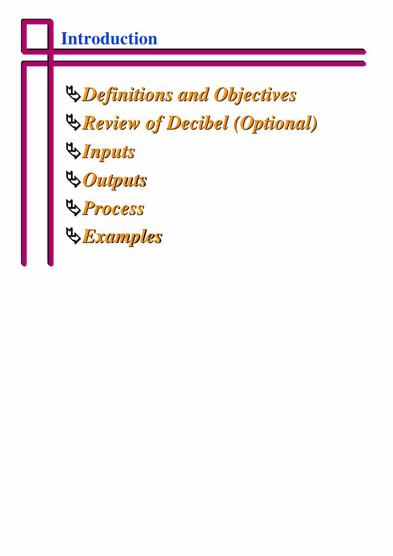
Introduction

ÄÄ Definitions and Objectives Definitions and Objectives

ÄÄ Review of Decibel (Optional) Review of Decibel (Optional)

ÄÄ Inputs Inputs

ÄÄOutputsOutputs

ÄÄ Process Process

ÄÄ Examples Examples



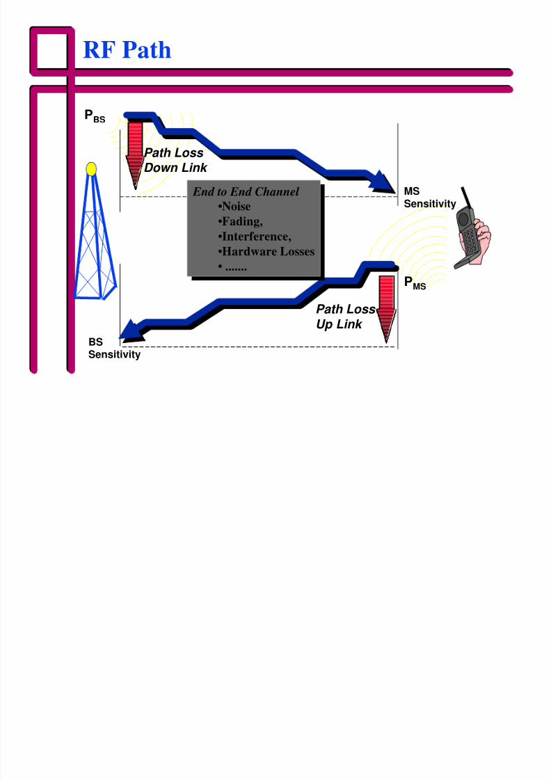
RF Path

BSSensitivity

MSSensitivity

Path Loss

Down Link

Path Loss

Up Link

PBS

PMS

End to End Channel •Noise

•Fading,

•Interference,

•Hardware Losses

• .......

End to End Channel •Noise

•Fading,

•Interference,

•Hardware Losses

• .......



Objectives and Definitions



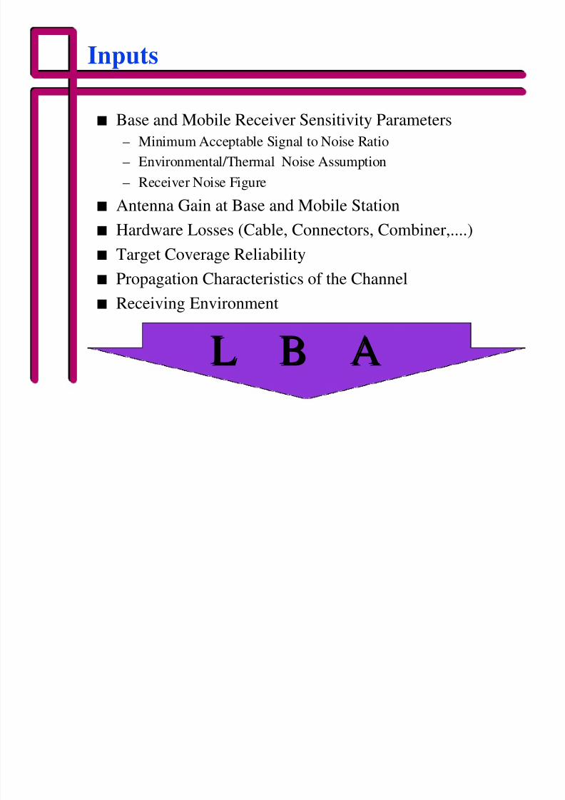
Inputs

n Base and Mobile Receiver Sensitivity Parameters

– Minimum Acceptable Signal to Noise Ratio

– Environmental/Thermal Noise Assumption

– Receiver Noise Figure

n Antenna Gain at Base and Mobile Station

n Hardware Losses (Cable, Connectors, Combiner,....)

n Target Coverage Reliability

n Propagation Characteristics of the Channel

n Receiving Environment

L B AL B A



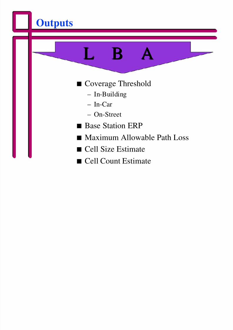
Outputs

n Coverage Threshold

– In-Building

– In-Car

– On-Street

n Base Station ERP

n Maximum Allowable Path Loss

n Cell Size Estimate

n Cell Count Estimate

L B AL B A



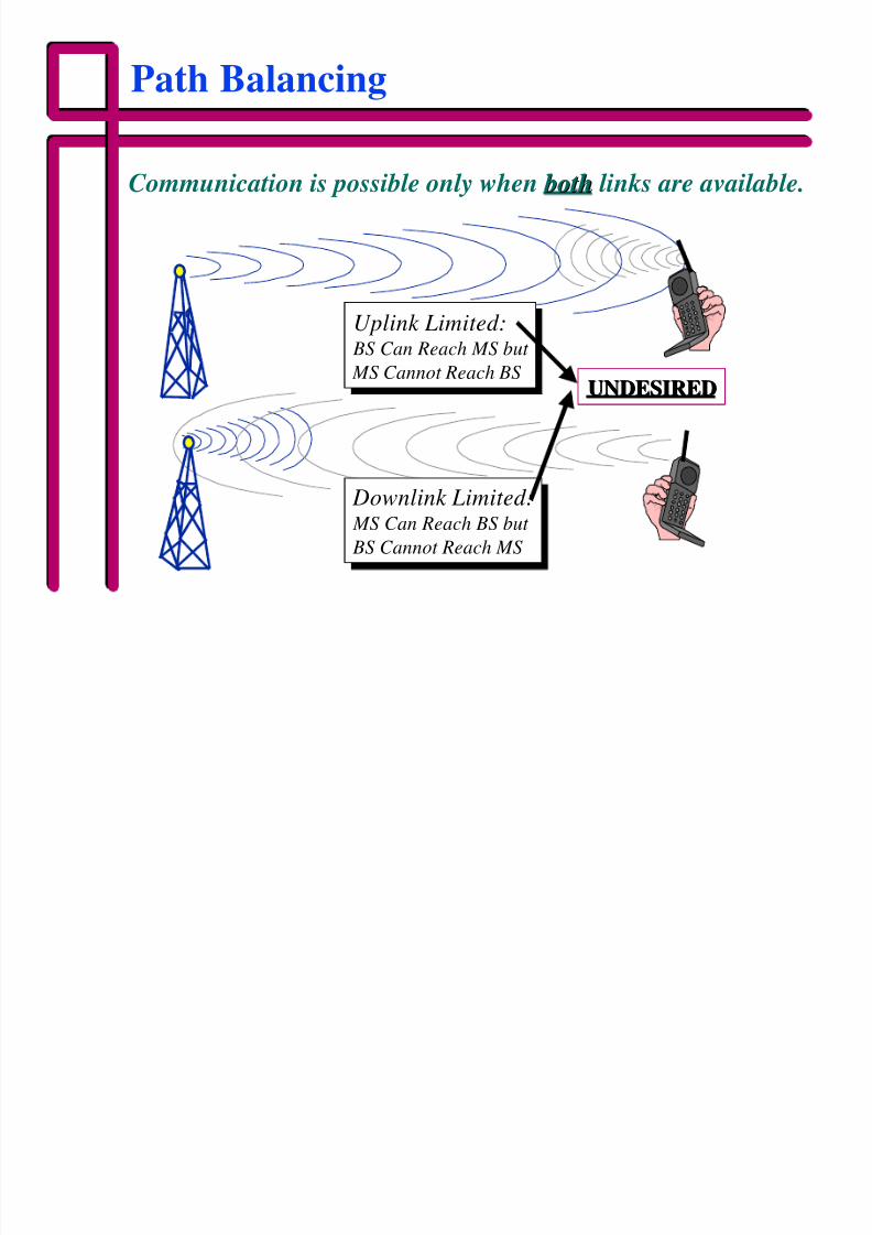
Path Balancing

Uplink Limited: BS Can Reach MS but

MS Cannot Reach BS

Uplink Limited: BS Can Reach MS but

MS Cannot Reach BS

Downlink Limited: MS Can Reach BS but

BS Cannot Reach MS

Downlink Limited: MS Can Reach BS but

BS Cannot Reach MS

Communication is possible only when both both links are available.

UNDESIREDUNDESIRED



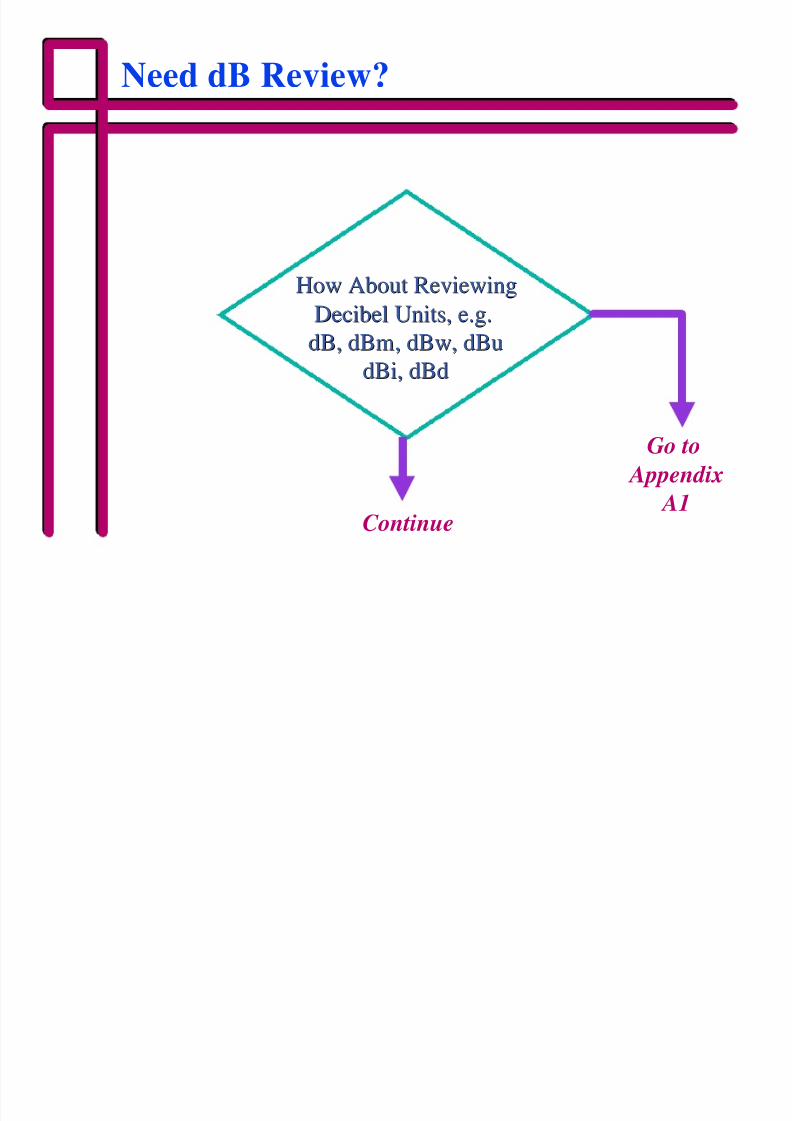
Need dB Review?

How About ReviewingHow About Reviewing

Decibel Units, e.g.Decibel Units, e.g.

dB,dB, dBmdBm,, dBwdBw,, dBudBu

dBidBi,, dBddBd

Go to

Appendix

A1Continue



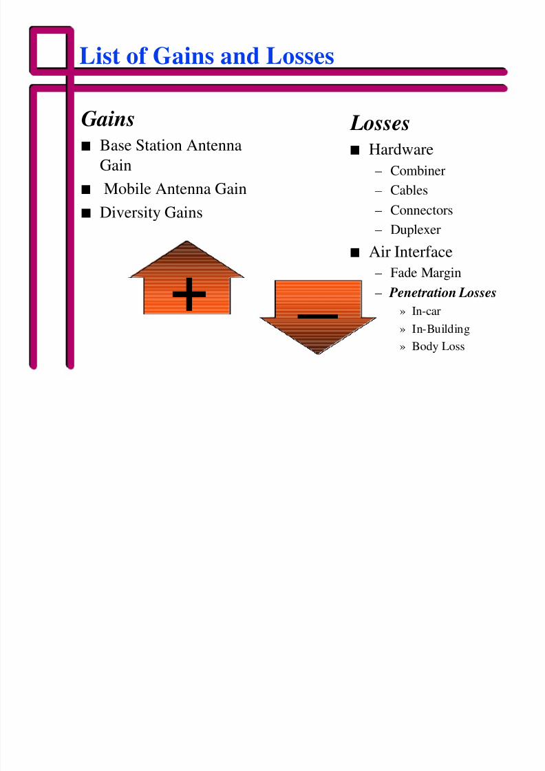
List of Gains and Losses

Gainsn Base Station Antenna

Gain

n Mobile Antenna Gainn Diversity Gains

Lossesn Hardware

– Combiner

– Cables– Connectors

– Duplexer

n Air Interface

– Fade Margin

– Penetration Losses

» In-car

» In-Building

» Body Loss

+ _



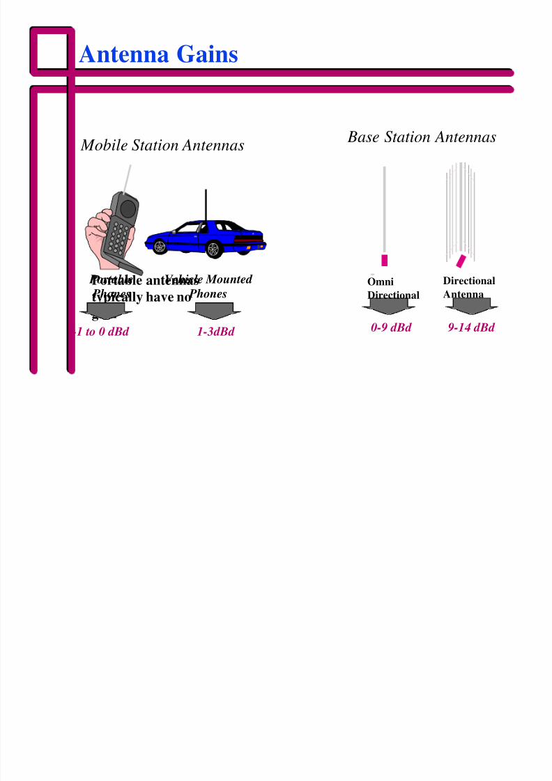
Antenna Gains

Portable antennas

typically have no

gain

Omni

Directional

Directional

Antenna

0-9 dBd 9-14 dBd

Base Station Antennas Mobile Station Antennas

Portable

Phones

Vehicle Mounted

Phones

-1 to 0 dBd 1-3dBd



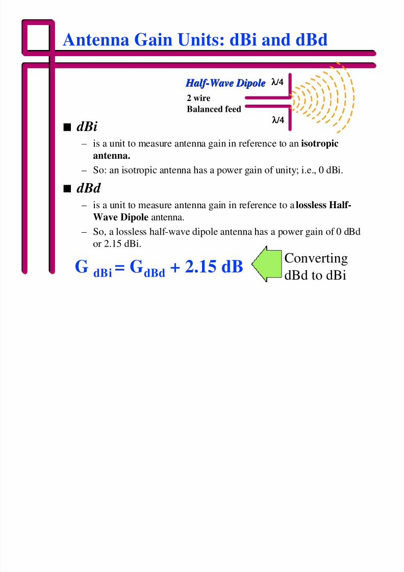
Antenna Gain Units: dBi and dBd

n dBi

– is a unit to measure antenna gain in reference to an isotropicantenna.

– So: an isotropic antenna has a power gain of unity; i.e., 0 dBi.

n dBd – is a unit to measure antenna gain in reference to a lossless Half-

Wave Dipole antenna.

– So, a lossless half-wave dipole antenna has a power gain of 0 dBd

or 2.15 dBi.

G dBi = GdBd + 2.15 dB

2 wire

Balanced feed

λ/4λ/4

λ/4λ/4

Half-Wave Dipole Half-Wave Dipole

Converting

dBd to dBi



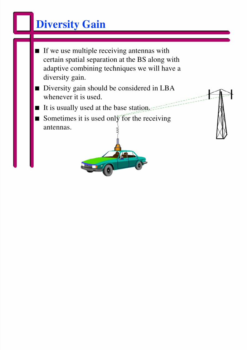
Diversity Gain

n If we use multiple receiving antennas with

certain spatial separation at the BS along with

adaptive combining techniques we will have a

diversity gain.

n Diversity gain should be considered in LBAwhenever it is used.

n It is usually used at the base station.

n Sometimes it is used only for the receiving

antennas.



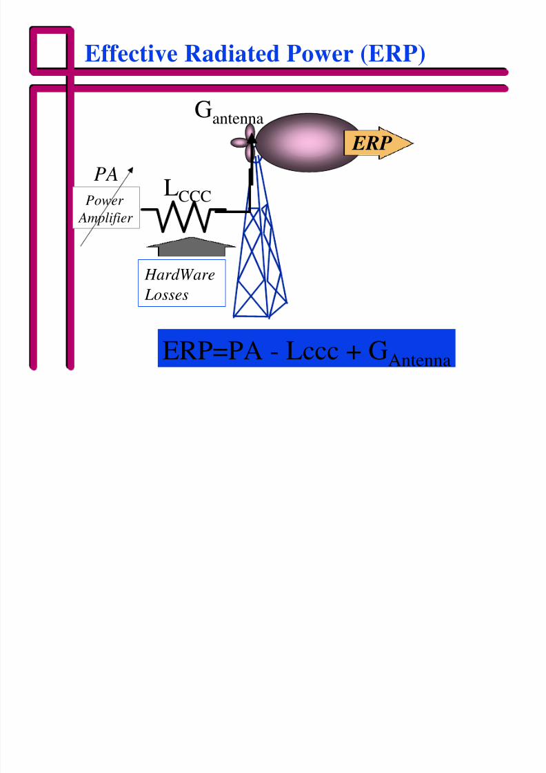
Effective Radiated Power (ERP)

Power

Amplifier

HardWare

Losses

PA

LCCC

Gantenna

ERP

ERP=PA - Lccc + GAntenna



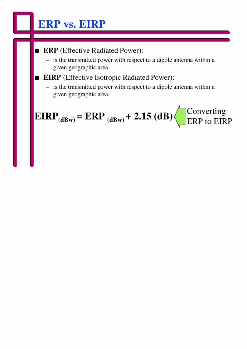
ERP vs. EIRP

n ERP (Effective Radiated Power):

– is the transmitted power with respect to a dipole antenna within a

given geographic area.

n EIRP (Effective Isotropic Radiated Power):

– is the transmitted power with respect to a dipole antenna within agiven geographic area.

Converting

ERP to EIRPEIRP(dBw) = ERP (dBw) + 2.15 (dB)



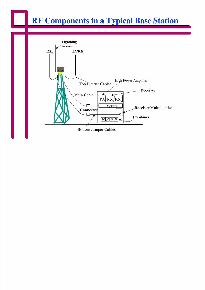
RF Components in a Typical Base Station

LNA

TX/RX2RX1

Lightning

Arrestor

PA RX1 RX2

Duplexer

Combiner

Top Jumper Cables

Main Cable

Connector Receiver Multicoupler

High Power Amplifier

Receiver

Bottom Jumper Cables



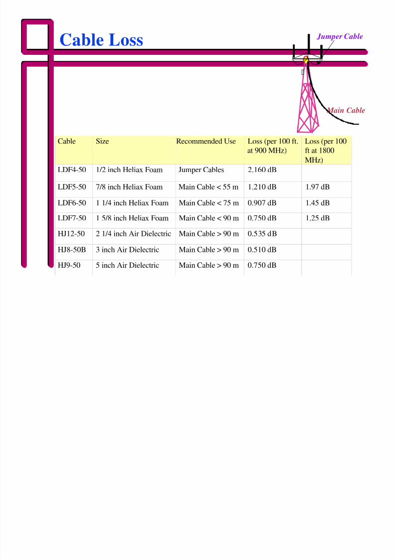
Cable Loss Jumper Cable

Main Cable

Cable Size Recommended Use Loss (per 100 ft.at 900 MHz)

Loss (per 100ft at 1800

MHz)

LDF4-50 1/2 inch Heliax Foam Jumper Cables 2.160 dB

LDF5-50 7/8 inch Heliax Foam Main Cable < 55 m 1.210 dB 1.97 dB

LDF6-50 1 1/4 inch Heliax Foam Main Cable < 75 m 0.907 dB 1.45 dB

LDF7-50 1 5/8 inch Heliax Foam Main Cable < 90 m 0.750 dB 1.25 dB

HJ12-50 2 1/4 inch Air Dielectric Main Cable > 90 m 0.535 dB

HJ8-50B 3 inch Air Dielectric Main Cable > 90 m 0.510 dB

HJ9-50 5 inch Air Dielectric Main Cable > 90 m 0.750 dB



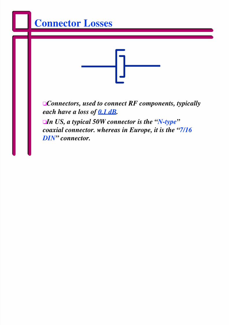
Connector Losses

oConnectors, used to connect RF components, typically

each have a loss of 0.1 dB .

o In US, a typical 50W connector is the “ N-type” coaxial connector. whereas in Europe, it is the “ 7/16

DIN ” connector.



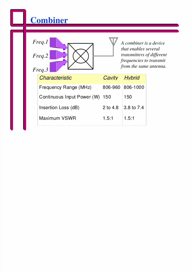
Combiner

Characteristic Cavity Hybrid

Frequency Range (MHz) 806-960 806-1000

Continuous Input Power (W) 150 150

Insertion Loss (dB) 2 to 4.8 3.8 to 7.4

Maximum VSWR 1.5:1 1.5:1

Freq.1

Freq.2

Freq.3

A combiner is a device

that enables several

transmitters of different

frequencies to transmit

from the same antenna.



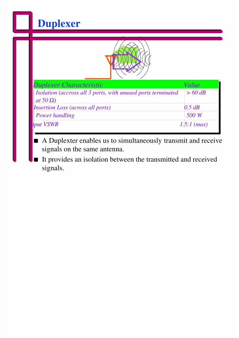
Duplexer

Duplexer Characteristic Value Isolation (accross all 3 ports, with unused ports terminated

at 50 Ω)

> 60 dB

Insertion Loss (across all ports) 0.5 dB

Power handling 500 W

Input VSWR 1.5:1 (max)

n A Duplexter enables us to simultaneously transmit and receive

signals on the same antenna.

n It provides an isolation between the transmitted and received

signals.



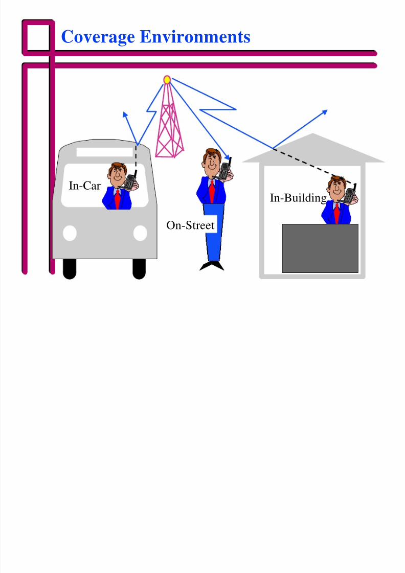
Coverage Environments

In-CarIn-Building

On-Street



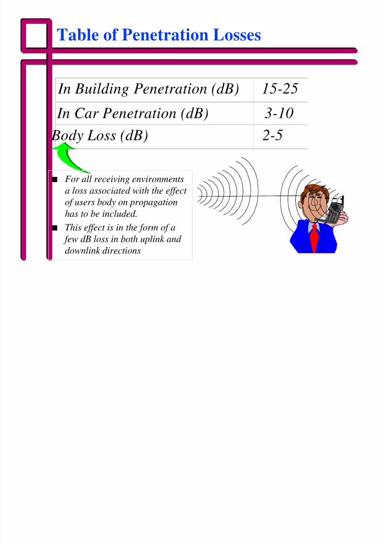
Table of Penetration Losses

In Building Penetration (dB) 15-25

In Car Penetration (dB) 3-10

Body Loss (dB) 2-5

n For all receiving environments

a loss associated with the effect

of users body on propagationhas to be included.

n This effect is in the form of a

few dB loss in both uplink and

downlink directions



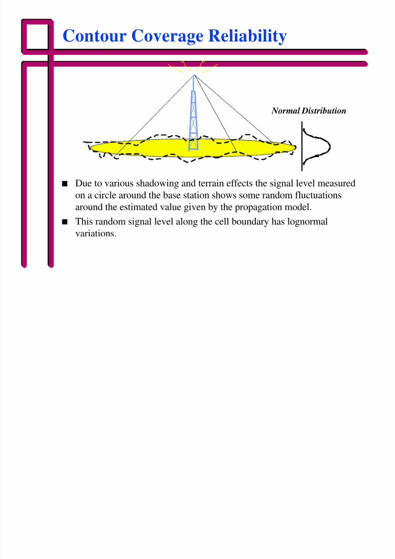
Contour Coverage Reliability

n Due to various shadowing and terrain effects the signal level measured

on a circle around the base station shows some random fluctuations

around the estimated value given by the propagation model.n This random signal level along the cell boundary has lognormal

variations.

Normal Distribution



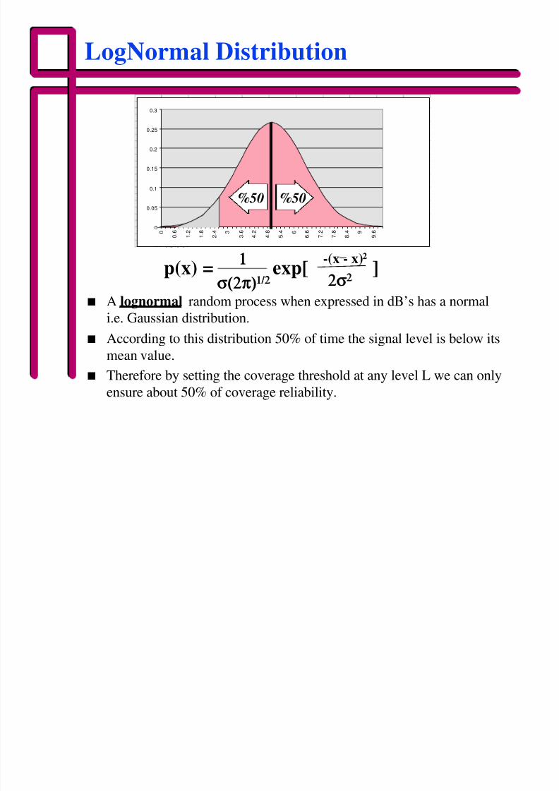
LogNormal Distribution

0 0.001031 1.50.2 0.001594 2

0.4 0.002420.6 0.00361

0.8 0.005291

1 0.0076171.2 0.010774

1.4 0.0149691.6 0.020432

1.8 0.027397

2 0.0360892.2 0.046702

2.4 0.0593692.6 0.074143

2.8 0.090962

3 0.109633.2 0.129801

3.4 0.1509743.6 0.172508

3.8 0.193644 0.21353

4.2 0.231314

4.4 0.246164

0

0.05

0.1

0.15

0.2

0.25

0.3

0

0 .

6

1 .

2

1 .

8

2 .

4 3

3 .

6

4 .

2

4 .

8

5 .

4 6

6 .

6

7 .

2

7 .

8

8 .

4 9

9 .

6

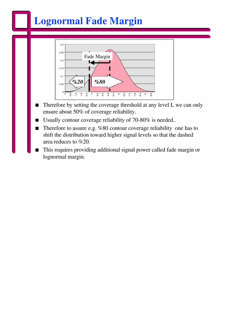
n A lognormal random process when expressed in dB’s has a normal

i.e. Gaussian distribution.

n According to this distribution 50% of time the signal level is below its

mean value.

n Therefore by setting the coverage threshold at any level L we can only

ensure about 50% of coverage reliability.

-(x - x)2_

p(x) = exp[ ]σ(2π)σ(2π)1/21/2 2σ2σ22

11

%50%50



Lognormal Fade Margin

0 0.001031 1.50.2 0.001594 2

0.4 0.002420.6 0.00361

0.8 0.005291

1 0.0076171.2 0.010774

1.4 0.0149691.6 0.020432

1.8 0.027397

2 0.0360892.2 0.046702

2.4 0.0593692.6 0.074143

2.8 0.090962

3 0.109633.2 0.129801

3.4 0.1509743.6 0.172508

3.8 0.193644 0.21353

4.2 0.231314

4.4 0.246164

0

0.05

0.1

0.15

0.2

0.25

0.3

0

0 .

6

1 .

2

1 .

8

2 .

4 3

3 .

6

4 .

2

4 .

8

5 .

4 6

6 .

6

7 .

2

7 .

8

8 .

4 9

9 .

6

n Therefore by setting the coverage threshold at any level L we can only

ensure about 50% of coverage reliability.

n Usually contour coverage reliability of 70-80% is needed..

n Therefore to assure e.g. %80 contour coverage reliability one has to

shift the distribution toward higher signal levels so that the dashed

area reduces to %20.

n This requires providing additional signal power called fade margin or

lognormal margin.

%20 %80

Fade Margin



Area Coverage Reliability

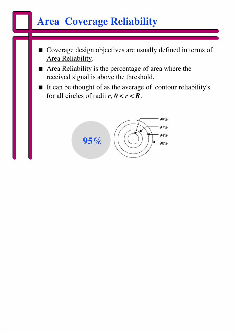
n Coverage design objectives are usually defined in terms of

Area Reliability.

n Area Reliability is the percentage of area where the

received signal is above the threshold.

n It can be thought of as the average of contour reliability's

for all circles of radii r, 0 < r < R.

99%

97%

94%

90%95%



From Area to Contour Reliability

0.5

0.55

0.6

0.65

0.7

0.75

0.8

0.85

0.9

0.95

1

σσ/n

A r e a R e l i a b i l i t y

0 1 2 3 4 5 6 7 8

P X 0(R) = 0.95

0.9

0.850.8

0.75

0.7

0.65

0.6

0.55

0.5

Area Reliability

σσ /nContour Reliability



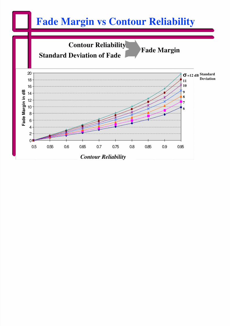
Fade Margin vs Contour Reliability

0

2

46

8

10

12

14

1618

20

0.5 0.55 0.6 0.65 0.7 0.75 0.8 0.85 0.9 0.95

Location Probability at Cell Edge

F a d e M a r g i n i n d B

σσ =12 dB

1110

9

8

7

6

Standard

Deviation

Contour Reliability

Contour Reliability

Standard Deviation of FadeFade Margin



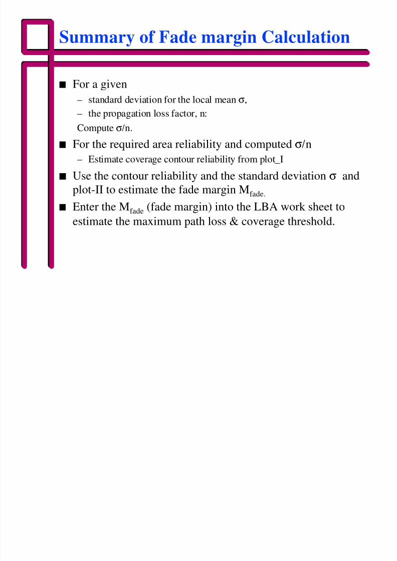
Summary of Fade margin Calculation

n For a given

– standard deviation for the local mean σ,

– the propagation loss factor, n:

Compute σ/n.

n For the required area reliability and computed σ/n– Estimate coverage contour reliability from plot_I

n Use the contour reliability and the standard deviation σ and

plot-II to estimate the fade margin Mfade.

n Enter the Mfade (fade margin) into the LBA work sheet toestimate the maximum path loss & coverage threshold.



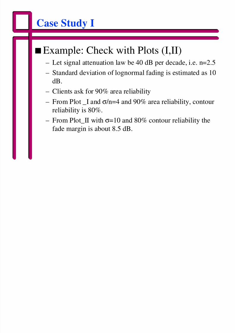
Case Study I

nExample: Check with Plots (I,II)– Let signal attenuation law be 40 dB per decade, i.e. n=2.5

– Standard deviation of lognormal fading is estimated as 10

dB.– Clients ask for 90% area reliability

– From Plot _I and σ /n=4 and 90% area reliability, contour

reliability is 80%.

– From Plot_II with σ=10 and 80% contour reliability the

fade margin is about 8.5 dB.



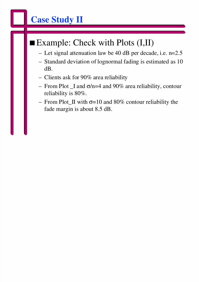
Case Study II

nExample: Check with Plots (I,II)– Let signal attenuation law be 40 dB per decade, i.e. n=2.5

– Standard deviation of lognormal fading is estimated as 10

dB.– Clients ask for 90% area reliability

– From Plot _I and σ /n=4 and 90% area reliability, contour

reliability is 80%.

– From Plot_II with σ=10 and 80% contour reliability the

fade margin is about 8.5 dB.



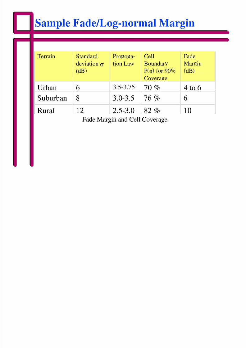
Sample Fade/Log-normal Margin

Terrain Standard

deviation σdB

Pro o a-

tion Law

Cell

Boundar

P n for 90%

Covera e

Fade

Mar in

dB

Urban 6 3.5-3.75 70 % 4 to 6Suburban 8 3.0-3.5 76 % 6

Rural 12 2.5-3.0 82 % 10Fade Margin and Cell Coverage



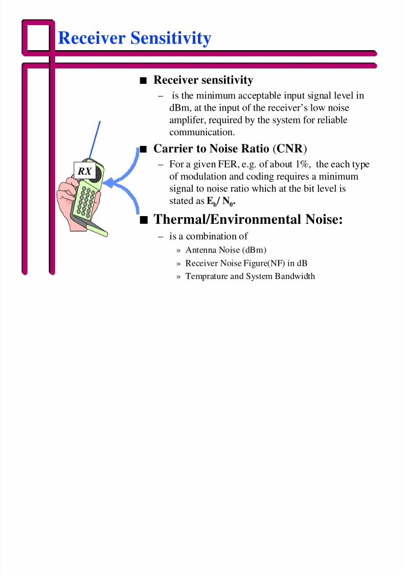
Receiver Sensitivity

n Receiver sensitivity

– is the minimum acceptable input signal level in

dBm, at the input of the receiver’s low noise

amplifer, required by the system for reliable

communication.

n Carrier to Noise Ratio (CNR)

– For a given FER, e.g. of about 1%, the each type

of modulation and coding requires a minimum

signal to noise ratio which at the bit level is

stated as Eb / N0.

n Thermal/Environmental Noise:– is a combination of

» Antenna Noise (dBm)

» Receiver Noise Figure(NF) in dB

» Temprature and System Bandwidth

RX



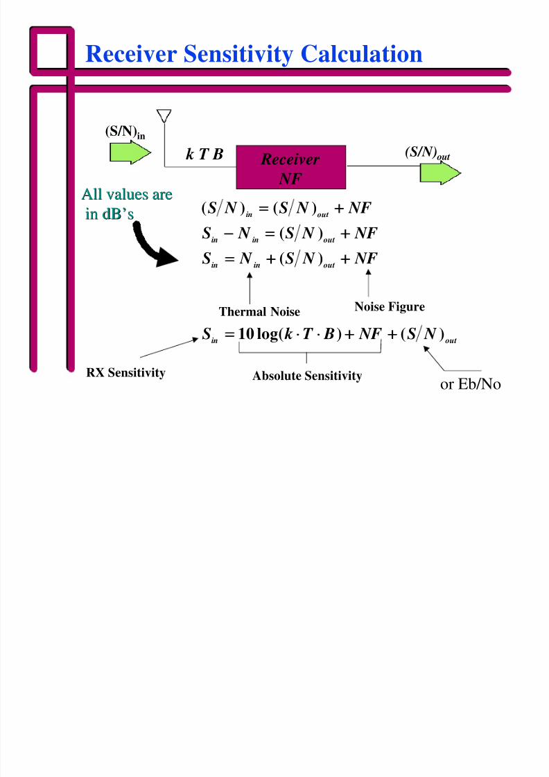
Receiver Sensitivity Calculation

Receiver

NF

k T B (S/N) out

(S/N)in

Thermal Noise Noise Figure

Absolute SensitivityRX Sensitivity

( ) ( )

( )

( )

log( ) ( )

S N S N NF

S N S N NF

S N S N NF

S k T B NF S N

in out

in in out

in in out

in out

== ++

−− == ++

== ++ ++

== ⋅⋅ ⋅⋅ ++ ++10

All values areAll values arein dB’sin dB’s

or Eb/No



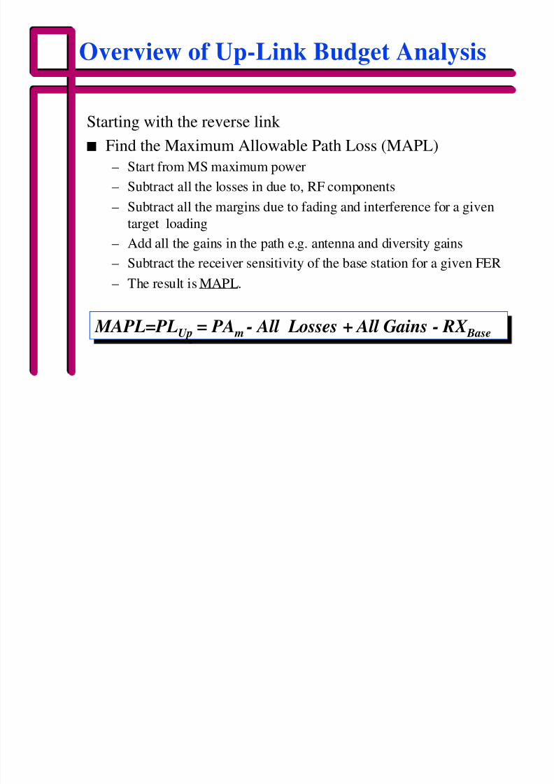
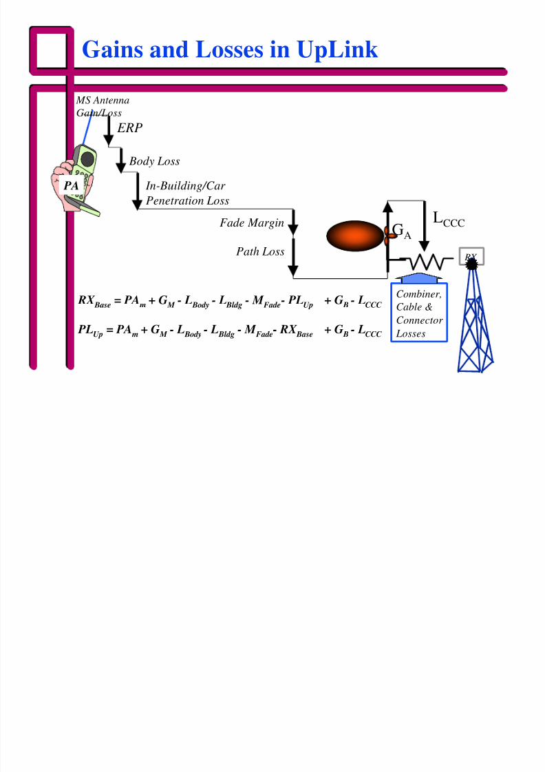
Overview of Up-Link Budget Analysis

Starting with the reverse link

n Find the Maximum Allowable Path Loss (MAPL)

– Start from MS maximum power

– Subtract all the losses in due to, RF components

– Subtract all the margins due to fading and interference for a given

target loading

– Add all the gains in the path e.g. antenna and diversity gains

– Subtract the receiver sensitivity of the base station for a given FER

– The result is MAPL.

MAPL=PLUp = PA m - All Losses + All Gains - RX Base MAPL=PLUp = PA m - All Losses + All Gains - RX Base



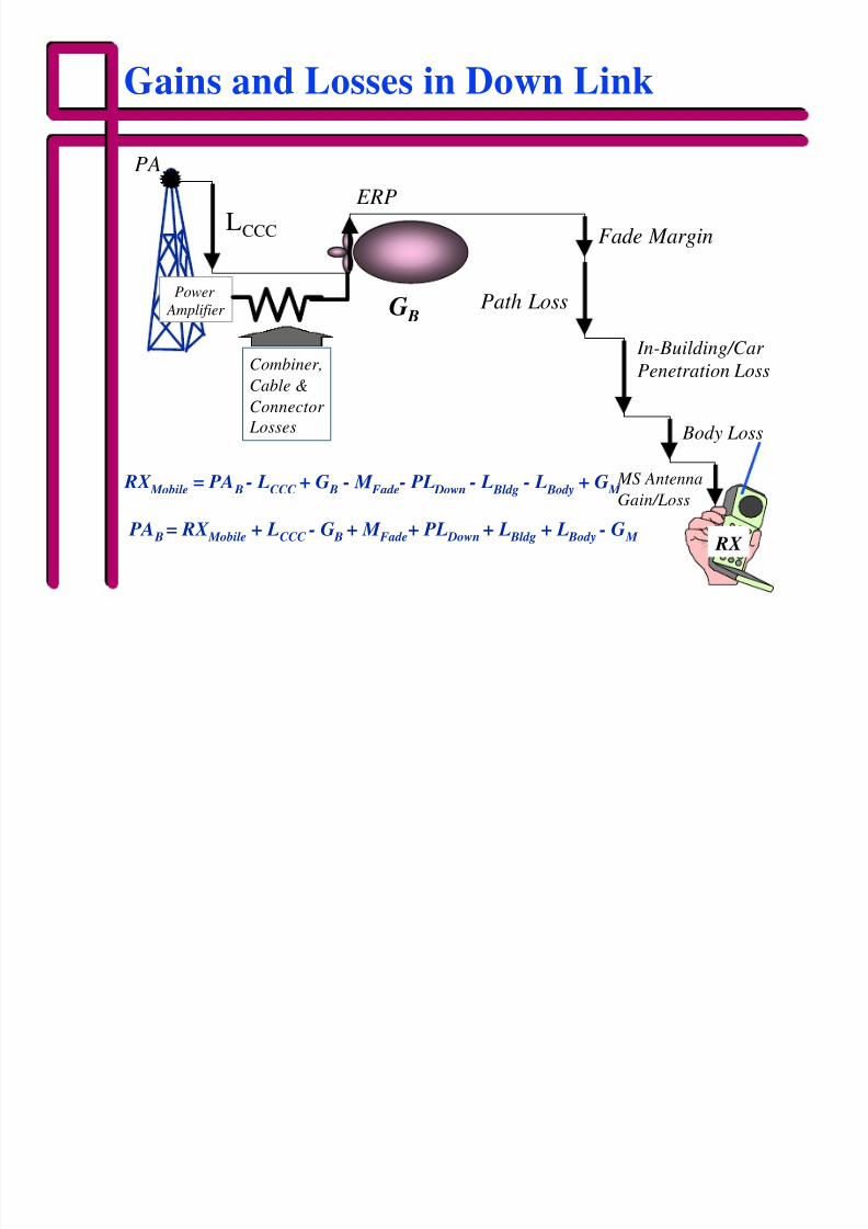
Overview of LBA Forward Link

In the forward link:

n For each channel

– Compute the MS sensitivity for a given Eb/No requirement

– Add the reverse link path loss and add a path imbalance if needed

– Add/subtract all losses/gains not considered in the reverse link calculations

– The result is ERP of base station



Gains and Losses in UpLink

LCCC

RX

Combiner,

Cable &

Connector

Losses

GA

Path Loss

Fade Margin

ERP

In-Building/Car

Penetration Loss

Body Loss

MS AntennaGain/Loss

PA

RX Base = PA m + G M - L Body - L Bldg - M Fade- PLUp + G B - LCCC

PLUp = PA m + G M - L Body - L Bldg - M Fade- RX Base + G B - LCCC



Gains and Losses in Down Link

Power

Amplifier

Combiner,

Cable &

Connector

Losses

PA

LCCC

G B Path Loss

Fade Margin

ERP

In-Building/Car

Penetration Loss

Body Loss

MS Antenna

Gain/Loss

RX

RX Mobile = PA B - LCCC + G B - M Fade- PL Down - L Bldg - L Body + G M

PA B = RX Mobile + LCCC - G B + M Fade+ PL Down + L Bldg + L Body - G M



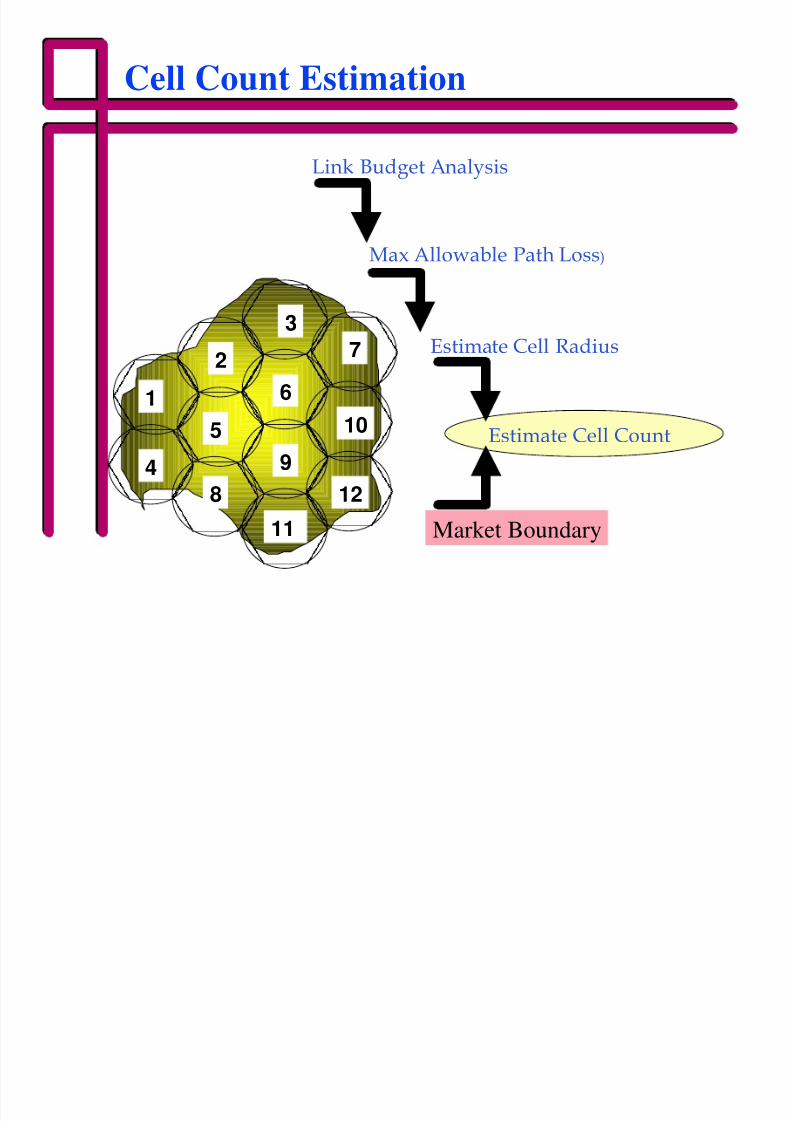
Cell Size/Count Estimation

n Objective:

– To determine the number of cells required to provide coverage for

a given area.

n Required Input:

– Maximum Allowable Path Loss (MAPL)– Propagation Loss Model



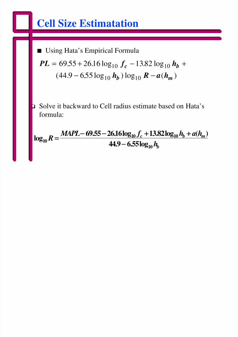
n Using Hata’s Empirical Formula

Cell Size Estimatation

o Solve it backward to Cell radius estimate based on Hata’s

formula:

PL f h

h R a h

c b

b m

= + − +

− −

69 55 26 16 13 82

44 9 6 55

10 10

10 10

. . log . log

( . . log ) log ( )

log. . log . log ( )

. . log10

10 10

10

69 55 2616 13 82

44 9 6 55 R

MAPL f h a h

h

c b m

b

==−− −− ++ ++

−−



Cell Count Estimation

1

2

3

4

5

7

6

9

8

10

12

11

Link Budget Analysis

Max Allowable Path Loss)

Estimate Cell Radius

Estimate Cell Count

Market Boundary



Outline



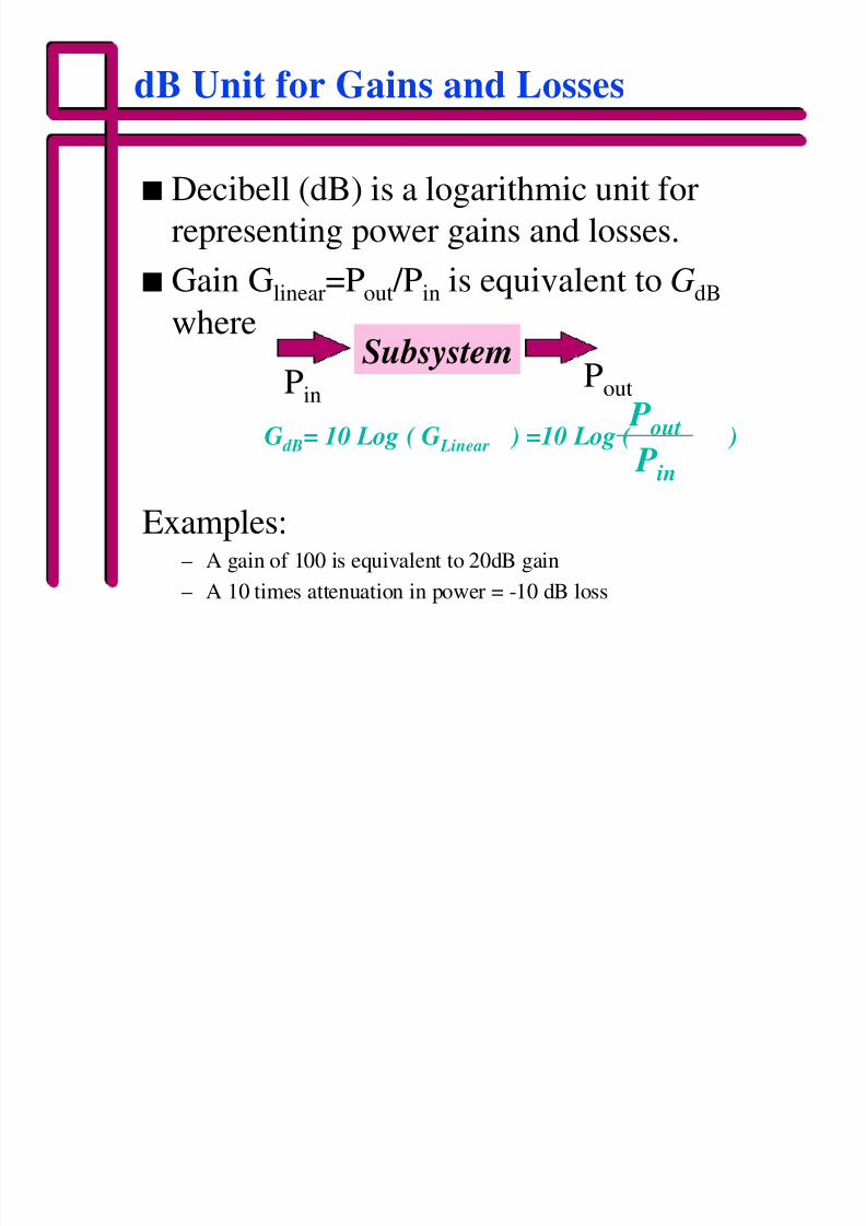
dB Unit for Gains and Losses

n Decibell (dB) is a logarithmic unit for

representing power gains and losses.

n Gain Glinear=Pout /Pin is equivalent to GdB

where

Examples:– A gain of 100 is equivalent to 20dB gain

– A 10 times attenuation in power = -10 dB loss

SubsystemPin

Pout

P out

Pin

G dB= 10 Log ( G Linear ) =10 Log ( )



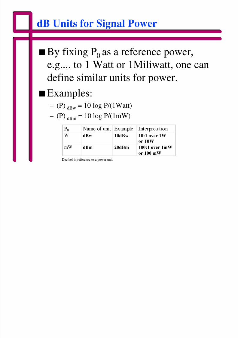
dB Units for Signal Power

nBy fixing P0 as a reference power,

e.g.... to 1 Watt or 1Miliwatt, one can

define similar units for power.

nExamples:– (P) dBw = 10 log P/(1Watt)

– (P) dBm = 10 log P/(1mW)

P0 Name of unit Example Interpretation

W dBw 10dBw 10:1 over 1W

or 10W

mW dBm 20dBm 100:1 over 1mW

or 100 mW

Decibel in reference to a power unit



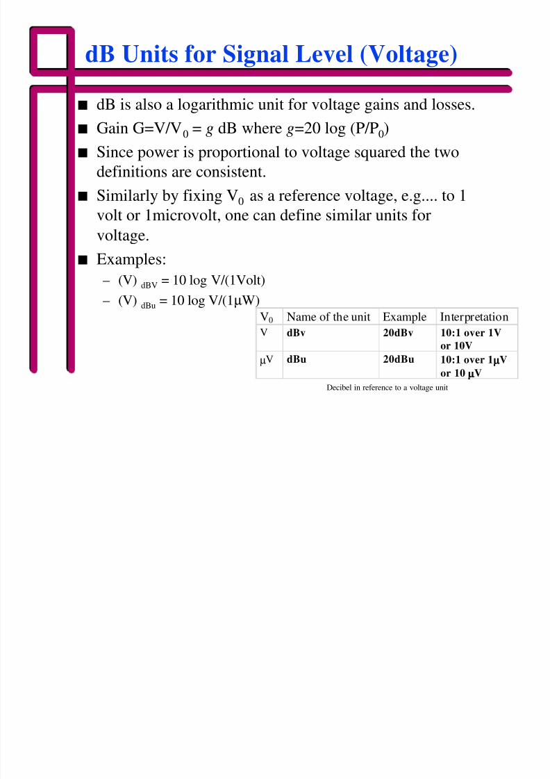
dB Units for Signal Level (Voltage)

n dB is also a logarithmic unit for voltage gains and losses.

n Gain G=V/V0 = g dB where g=20 log (P/P0)

n Since power is proportional to voltage squared the two

definitions are consistent.

n Similarly by fixing V0 as a reference voltage, e.g.... to 1volt or 1microvolt, one can define similar units for

voltage.

n Examples:

– (V) dBV = 10 log V/(1Volt)

– (V) dBu = 10 log V/(1µW)

V0 Name of the unit Example Interpretation

V dBv 20dBv 10:1 over 1V

or 10V

µV dBu 20dBu 10:1 over 1µµV

or 10 µµV

Decibel in reference to a voltage unit



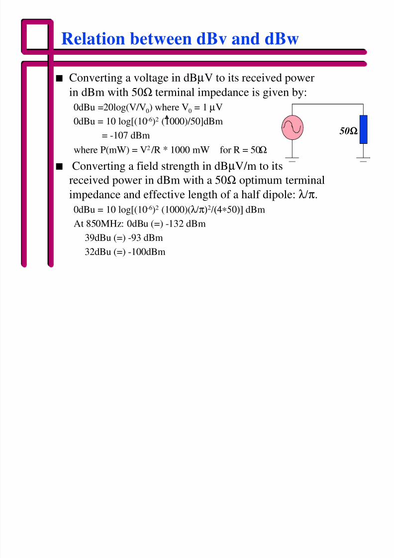
Relation between dBv and dBw

n Converting a voltage in dBµV to its received power

in dBm with 50Ω terminal impedance is given by:

0dBu =20log(V/V0) where V0 = 1 µV

0dBu = 10 log[(10-6)2 (1000)/50]dBm

= -107 dBm

where P(mW) = V2 /R * 1000 mW for R = 50Ω

n Converting a field strength in dBµV/m to its

received power in dBm with a 50Ω optimum terminal

impedance and effective length of a half dipole: λ/π.

0dBu = 10 log[(10-6)2 (1000)(λ/π)2/(4∗50)] dBmAt 850MHz: 0dBu (=) -132 dBm

39dBu (=) -93 dBm

32dBu (=) -100dBm

50ΩΩ



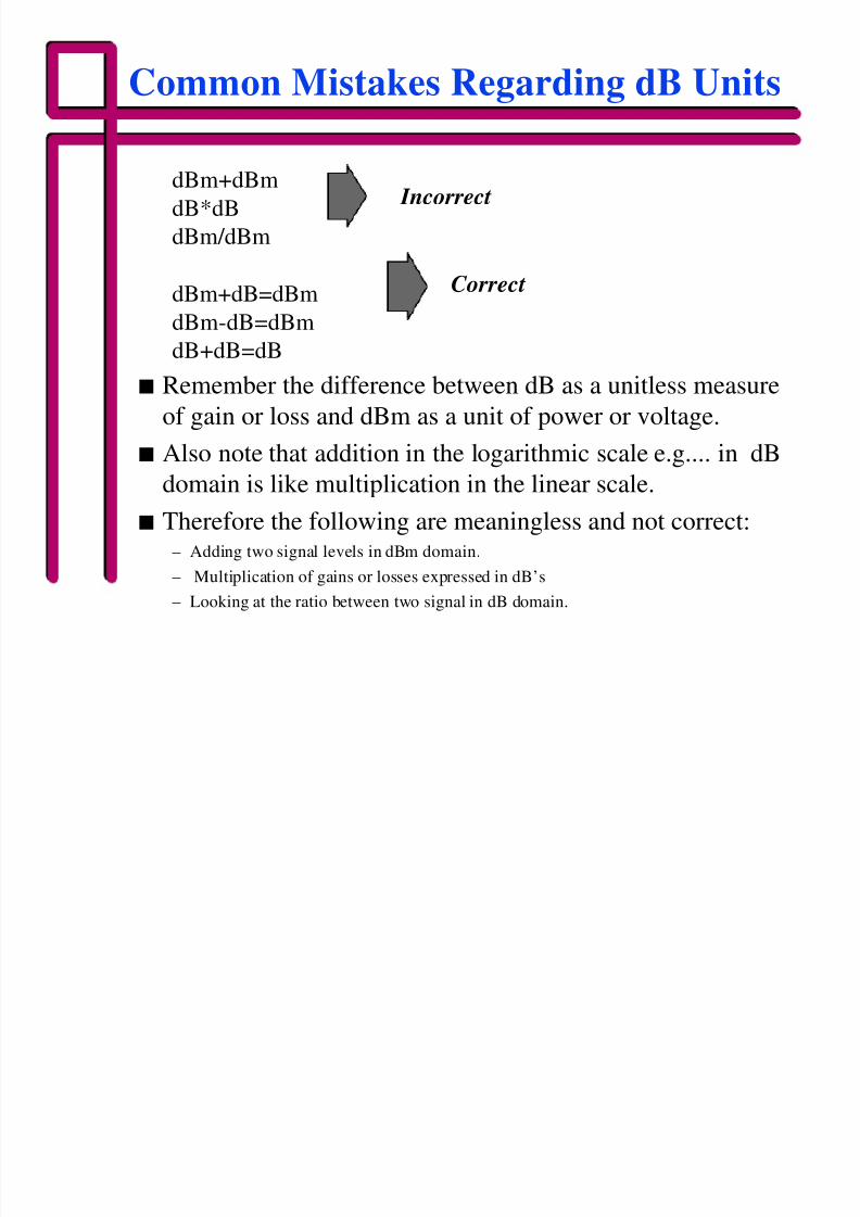
Common Mistakes Regarding dB Units

n Remember the difference between dB as a unitless measure

of gain or loss and dBm as a unit of power or voltage.

n Also note that addition in the logarithmic scale e.g.... in dBdomain is like multiplication in the linear scale.

n Therefore the following are meaningless and not correct:– Adding two signal levels in dBm domain.

– Multiplication of gains or losses expressed in dB’s

– Looking at the ratio between two signal in dB domain.

dBm+dBm

dB*dB

dBm/dBm

dBm+dB=dBm

dBm-dB=dBm

dB+dB=dB

Incorrect

Correct



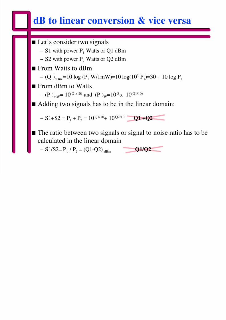
n Let’s consider two signals– S1 with power P1 Watts or Q1 dBm

– S2 with power P2 Watts or Q2 dBm

n From Watts to dBm

– (Q1)dBm =10 log (P1 W/1mW)=10 log(103 P1)=30 + 10 log P1

n From dBm to Watts

– (P1)mW= 10(Q1/10) and (P1)W=10-3 x 10(Q1/10)

n Adding two signals has to be in the linear domain:

– S1+S2 = P1 + P2 = 10Q1/10

+ 10Q2/10

Q1 +Q2

n The ratio between two signals or signal to noise ratio has to be

calculated in the linear domain

– S1/S2= P1 / P2 = (Q1-Q2) dBm Q1/Q2

dB to linear conversion & vice versa

Documents

Link Budget Analysis (WFI)