Linearly Parameterized Bandits

Paat Rusmevichientong John N. Tsitsiklis

Cornell University MIT

paatrus@cornell.edu jnt@mit.edu

January 18, 2010 @ 11:04pm

Abstract

We consider bandit problems involving a large (possibly infinite) collection of arms, in which

the expected reward of each arm is a linear function of an r-dimensional random vector Z ∈ Rr,

where r ≥ 2. The objective is to minimize the cumulative regret and Bayes risk. When the set of

arms corresponds to the unit sphere, we prove that the regret and Bayes risk is of order Θ(r√T ),

by establishing a lower bound for an arbitrary policy, and showing that a matching upper bound is

obtained through a policy that alternates between exploration and exploitation phases. The phase-

based policy is also shown to be effective if the set of arms satisfies a strong convexity condition.

For the case of a general set of arms, we describe a near-optimal policy whose regret and Bayes

risk admit upper bounds of the form O(r√T log3/2 T ).

Original Submission: January 19, 2009

1. Introduction

Since its introduction by Thompson (1933), the multiarmed bandit problem has served as an

important model for decision making under uncertainty. Given a set of arms with unknown reward

profiles, the decision maker must choose a sequence of arms to maximize the expected total payoff,

where the decision in each period may depend on the previously observed rewards. The multiarmed

bandit problem elegantly captures the tradeoff between the need to exploit arms with high payoff

and the incentive to explore previously untried arms for information gathering purposes.

Much of the previous work on the multiarmed bandit problem assumes that the rewards of the

arms are statistically independent (see, for example, Lai and Robbins (1985) and Lai (1987)). This

1

assumption enables us to consider each arm separately, but it leads to policies whose regret scales

linearly with the number of arms. Most policies that assume independence require each arm to be

tried at least once, and are impractical in settings involving many arms. In such settings, we want

a policy whose regret is independent of the number of arms.

When the mean rewards of the arms are assumed to be independent random variables, Lai

and Robbins (1985) show that the regret under an arbitrary policy must increase linearly with the

number of arms. However, the assumption of independence is quite strong in practice. In many

applications, the information obtained from pulling one arm can change our understanding of other

arms. For instance, in marketing applications, we expect a priori that similar products should have

similar sales. By exploiting the correlation among products/arms, we should be able to obtain a

policy whose regret scales more favorably than traditional bandit algorithms that ignore correlation

and assume independence.

Mersereau et al. (2008) propose a simple model that demonstrates the benefits of exploiting

the underlying structure of the rewards. They consider a bandit problem where the expected

reward of each arm is a linear function of an unknown scalar, with a known prior distribution.

Since the reward of each arm depends on a single random variable, the mean rewards are perfectly

correlated. They prove that, under certain assumptions, the cumulative Bayes risk over T periods

(defined below) under a greedy policy admits an O (log T ) upper bound, independent of the number

of arms.

In this paper, we extend the model of Mersereau et al. (2008) to the setting where the expected

reward of each arm depends linearly on a multivariate random vector Z ∈ Rr. We concentrate on

the case where r ≥ 2, which is fundamentally different from the previous model because the mean

rewards now depend on more than one random variable, and thus, they are no longer perfectly

correlated. The bounds on the regret and Bayes risk and the policies found in Mersereau et al.

(2008) no longer apply. To give a flavor for the differences, we will show that, in our model, the

cumulative Bayes risk under an arbitrary policy is at least Ω(r√T ), which is significantly higher

than the upper bound of O(log T ) attainable when r = 1.

The linearly parameterized bandit is an important model that has been studied by many re-

searchers, including Ginebra and Clayton (1995), Abe and Long (1999), and Auer (2002). The

results in this paper complement and extend the earlier and independent work of Dani et al.

(2008a) in a number of directions. We provide a detailed comparison between our work and the

existing literature in Sections 1.3 and 1.4.

2

1.1 The Model

We have a compact set Ur ⊂ Rr that corresponds to the set of arms, where r ≥ 2. The reward Xut

of playing arm u ∈ Ur in period t is given by

Xut = u′Z +Wu

t , (1)

where u′Z is the inner product between the vector u ∈ Ur and the random vector Z ∈ Rr. We

assume that the random variables Wut are independent of each other and of Z. Moreover, for

each u ∈ Ur, the random variables Wut : t ≥ 1 are identically distributed, with E [Wu

t ] = 0 for

all t and u. We allow the error random variables Wut to have unbounded support, provided that

their moment generating functions satisfy certain conditions (given in Assumption 1). Each vector

u ∈ Ur simultaneously represents an arm and determines the expected reward of that arm. So,

when it is clear from the context, we will interchangeably refer to a u ∈ Ur as either a vector or an

arm.

Let us introduce the following conventions and notation that will be used throughout the paper.

We denote vectors and matrices in bold. All vectors are column vectors. For any vector v ∈ Rr,

its transpose is denoted by v′, and is always a row vector. Let 0 denote the zero vector, and

for k = 1, . . . , r, let ek = (0, . . . , 1, . . . , 0) denote the standard unit vector in Rr, with a 1 in the

kth component and a 0 elsewhere. Also, let Ik denote the k × k identity matrix. We let A′ and

det(A) denote the transpose and determinant of A, respectively. If A is a symmetric positive

semidefinite matrix, then λmin(A) and λmax(A) denote the smallest and the largest eigenvalues of

A, respectively. We use A1/2 to denote its symmetric nonnegative definite square root, so that

A1/2A1/2 = A. If A is also positive definite, we let A−1/2 =(A−1

)1/2. For any vector v, ‖v‖ =√

v′v denotes the standard Euclidean norm, and for any positive definite matrix A, ‖v‖A =√

v′Av

denotes a corresponding weighted norm. For any two symmetric positive semidefinite matrices A

and B, we write A ≤ B if the matrix B −A is positive semidefinite. Also, all logarithms log(·)

in the paper denote the natural log, with base e. A random variable is denoted by an uppercase

letter while its realized values are denoted in lowercase.

For any t ≥ 1, let Ht−1 denote the set of possible histories until the end of period t − 1. A

policy ψ = (ψ1, ψ2, . . .) is a sequence of functions such that ψt : Ht−1 → Ur selects an arm in period

t based on the history until the end of period t − 1. For any policy ψ and z ∈ Rr, the T -period

cumulative regret under ψ given Z = z, denoted by Regret(z, T, ψ), is defined by

Regret(z, T, ψ) =T∑t=1

E

[maxv∈Ur

v′z−U′tz∣∣∣ Z = z

],

3

where for any t ≥ 1, Ut ∈ Ur is the arm chosen under ψ in period t. Since Ur is compact,

maxv∈Ur v′z is well defined for all z. The T -period cumulative Bayes risk under ψ is defined by

Risk(T, ψ) = E [Regret(Z, T, ψ)] ,

where the expectation is taken with respect to the prior distribution of Z. We aim to develop a

policy that minimizes the cumulative regret and Bayes risk. We note that minimizing the T -period

cumulative Bayes risk is equivalent to maximizing the expected total reward over T periods.

To facilitate exposition, when we discuss a particular policy, we will drop the superscript and

write Xt and Wt to denote XUtt and WUt

t , respectively, where Ut is the arm chosen by the policy

in period t. With this convention, the reward obtained in period t under a particular policy is

simply Xt = U′tZ +Wt.

1.2 Potential Applications

Although our paper focuses on a theoretical analysis, we mention briefly potential applications

to problems in marketing and revenue management. Suppose we have m arms indexed by Ur =

u1,u2, . . . ,um ⊂ Rr. For k = 1, . . . , r, let φk = (u1,k, u2,k, . . . , um,k) ∈ Rm denote an m-

dimensional column vector consisting of the kth coordinates of the different vectors u`. Let

µ = (µ1, . . . , µm) be the column vector consisting of expected rewards, where µ` denotes the

expected reward of arm u`. Under our formulation, the vector µ lies in an r-dimensional subspace

spanned by the vectors φ1, . . . ,φr, that is, µ =∑r

k=1 Zkφk, where Z = (Z1, . . . , Zr). If each arm

corresponds to a product to be offered to a customer, we can then interpret the vector φk as a fea-

ture vector or basis function, representing a particular characteristic of the products such as price

or popularity. We can then interpret the random variables Z1, . . . , Zr as regression coefficients,

obtained from approximating the vector of expected rewards using the basis functions φ1, . . . ,φr,

or more intuitively, as the weights associated with the different characteristics. Given a prior on the

coefficients Zk, our goal is to choose a sequence of products that gives the maximum expected total

reward. This representation suggests that our model might be applicable to problems where we

can approximate high-dimensional vectors using a linear combination of a few basis functions, an

approach that has been successfully applied to high-dimensional dynamic programming problems

(see Bertsekas and Tsitsiklis (1996) for an overview).

1.3 Related Literature

The multiarmed bandit literature can be divided into two streams, depending on the objective

function criteria: maximizing the total discounted reward over an infinite horizon or minimizing

the cumulative regret and Bayes risk over a finite horizon. Our paper focuses exclusively on the

4

second criterion. Much of the work in this area focuses on understanding the rate with which the

regret and risk under various policies increase over time. In their pioneering work, Lai and Robbins

(1985) establish an asymptotic lower bound of Ω(m log T ) for the T -period cumulative regret for

bandit problems with m independent arms whose mean rewards are “well-separated,” where the

difference between the expected reward of the best and second best arms is fixed and bounded

away from zero. They further demonstrate a policy whose regret asymptotically matches the lower

bound. In contrast, our paper focuses on problems where the number of arms is large (possibly

infinite), and where the gap between the maximum expected reward and the expected reward of

the second best arm can be arbitrarily small. Lai (1987) extends these results to a Bayesian setting,

with a prior distribution on the reward characteristics of each arm. He shows that when we have m

arms, the T -period cumulative Bayes risk is of order Θ(m log2 T ), when the prior distribution has a

continuous density function satisfying certain properties (see Theorem 3 in Lai, 1987). Subsequent

papers along this line include Agrawal et al. (1989), Agrawal (1995), and Auer et al. (2002).

There has been relatively little research, however, on policies that exploit the dependence among

the arms. Thompson (1933) allows for correlation among arms in his initial formulation, though he

only analyzes a special case involving independent arms. Robbins (1952) formulates a continuum-

armed bandit regression problem, but does not provide an analysis of the regret or risk. Berry and

Fristedt (1985) allow for dependence among arms in their formulation in Chapter 2, but mostly

focus on the case of independent arms. Feldman (1962) and Keener (1985) consider two-armed

bandit problems with two hidden states, where the rewards of each arm depend on the underlying

state that prevails. Pressman and Sonin (1990) formulate a general multiarmed bandit problem

with an arbitrary number of hidden states, and provide a detailed analysis for the case of two hidden

states. Pandey et al. (2007) study bandit problems where the dependence of the arm rewards is

represented by a hierarchical model.

A somewhat related literature on bandits with dependent arms is the recent work by Wang

et al. (2005a,b) and Goldenshluger and Zeevi (2007, 2008) who consider bandit problems with two

arms, where the expected reward of each arm depends on an exogenous variable that represents

side information. These models, however, differ from ours because they assume that the side

information variables are independent and identically distributed over time, and moreover, these

variables are perfectly observed before we choose which arm to play. In contrast, we assume that

the underlying random vector Z is unknown and fixed over time, to be estimated based on past

rewards and decisions.

Our formulation can be viewed as a sequential method for maximizing a linear function based

on noisy observations of the function values, and it is thus closely related to the field of stochastic

5

approximation, which was developed by Robbins and Monro (1951) and Kiefer and Wolfowitz

(1952). We do not provide a comprehensive review of the literature here; interested readers are

referred to an excellent survey by Lai (2003). In stochastic approximation, we wish to find an

adaptive sequence Ut ∈ Rr : t ≥ 1 that converges to a maximizer u∗ of a target function, and

the focus is on establishing the rate at which the mean squared error E[‖Ut − u∗‖2

]converges

to zero (see, for example, Blum, 1954 and Cicek et al., 2009). In contrast, our cumulative regret

and Bayes risk criteria take into account the cost associated with each observation. The different

performance measures used in our formulation lead to entirely different policies and performance

characteristics.

Our model generalizes the “response surface bandits” introduced by Ginebra and Clayton

(1995), who assume a normal prior on Z and provide a simple tunable heuristic, without any

analysis on the regret or risk. Abe and Long (1999), Auer (2002), and Dani et al. (2008a) all

consider a special case of our model where the random vector Z and the error random variables

Wut are bounded almost surely, and with the exception of the last paper, focus on the regret cri-

terion. Abe and Long (1999) demonstrate a class of bandits where the dimension r is at least

Ω(√T ), and show that the T -period regret under an arbitrary policy must be at least Ω

(T 3/4

).

Auer (2002) describes an algorithm based on least squares estimation and confidence bounds, and

establishes an O(√

r√T log3/2 (T |Ur|)

)upper bound on the regret, for the case of finitely many

arms. Dani et al. (2008a) show that the policy of Auer (2002) can be extended to problems having

an arbitrary compact set of arms, and also make use of a barycentric spanner. They establish

an O(r√T log3/2 T ) upper bound on the regret, and discuss a variation of the policy that is more

computationally tractable (at the expense of higher regret). Dani et al. (2008a) also establish an

Ω(r√T ) lower bound on the Bayes risk when the set of arms is the Cartesian product of circles1.

However, this leaves a O(log3/2 T ) gap from the upper bound, leaving open the question of the

exact order of regret and risk.

1.4 Contributions and Organizations

One of our contributions is proving that the regret and Bayes risk for a broad class of linearly

parameterized bandits is of order Θ(r√T ). In Section 2, we establish an Ω(r

√T ) lower bound

for an arbitrary policy, when the set of arms is the unit sphere in Rr. Then, in Section 3, we

show that a matching O(r√T ) upper bound can be achieved through a phase-based policy that

alternates between exploration and exploitation phases. To the best of our knowledge, this is the

first result that establishes matching upper and lower bounds for a class of linearly parameterized

1The original lower bound (Theorem 3 on page 360 of Dani et al., 2008a) was not entirely correct; a correct version

was provided later, in Dani et al. (2008b).

6

bandits. Table 1 summarizes our results and provides a comparison with the results in Mersereau

et al. (2008) for the case r = 1. In the ensuing discussion of the bounds, we focus on the main

parameters, r and T , with more precise statements given in the theorems.

Although we obtain the same lower bound of Ω(r√T ), our example and proof techniques are

very different from Dani et al. (2008a). We consider the unit sphere, with a multivariate normal

prior on Z, and standard normal errors. The analysis in Section 2 also illuminates the behavior of

the least mean squares estimator in this setting, and we believe that it provides an approach that

can be used to address more general classes of linear estimation and adaptive control problems.

We also prove that the phase-based policy remains effective (that is, admits an O(r√T ) upper

bound) for a broad class of bandit problems in which the set of arms is strongly convex2 (defined

in Section 3). To our knowledge, this is the first result that establishes the connection between

a geometrical property (strong convexity) of the underlying set of arms and the effectiveness of

separating exploration from exploitation. We suspect that strong convexity may have similar

implications for other types of bandit and learning problems.

When the set of arms is an arbitrary compact set, the separation of exploration and exploitation

may not be effective, and we consider in Section 4 an active exploration policy based on least squares

estimation and confidence regions. We prove that the regret and risk under this policy are bounded

above by O(r√T log3/2 T ), which is within a logarithmic factor of the lower bound. Our policy is

closely related to the one considered in Auer (2002) and further analyzed in Dani et al. (2008a),

with differences in a number of respects. First, our model allows the random vector Z and the

errors Wut to have unbounded support, which requires a somewhat more complicated analysis.

Second, our policy is an “anytime” policy, in the sense that the policy does not depend on the

time horizon T of interest. In contrast, the policies of Auer (2002) and Dani et al. (2008a) involve

a certain parameter δ whose value must be set in advance as a function of the time horizon T in

order to obtain the O(r√T log3/2 T

)regret bound.

We finally comment on the case where the set of arms is finite and fixed. We show that the

regret and risk under our active exploration policy increase gracefully with time, as log T and log2 T ,

respectively. These results show that our policy is within a constant factor of the asymptotic lower

bounds established by Lai and Robbins (1985) and Lai (1987). In contrast, for the policies of Auer

(2002) and Dani et al. (2008a), the available regret upper bounds grow over time as√T log3/2 T

and log3 T , respectively.

2One can show that the Cartesian product of circles is not strongly convex, and thus, our phase-based policy cannot

be applied to give the matching upper bound for the example used in Dani et al. (2008a).

7

T -period Cumulative Regret T -period Cumulative Bayes Risk

Dimension Set of

(r) Arms (Ur)Lower Bound Upper Bound Lower Bound Upper Bound

r = 1 Any Compact Set Ω“√

T”

O“√

T”

Ω (log T ) O (log T )

(Mersereau et al., 2008)

Unit Sphere Ω“r√

T”

O“r√

T”

Ω“r√

T”

O“r√

T”

r ≥ 2 (Sections 2 and 3)

(This Paper)

Any Compact Set Ω“r√

T”

O“r√

T log3/2 T”

Ω“r√

T”

O“r√

T log3/2 T”

(Section 4)

Table 1: Regret and risk bounds for various values of r and for different collections of arms.

We note that the bounds on the cumulative Bayes risk given in Table 1 hold under certain

assumptions on the prior distribution of the random vector Z. For r = 1, Z is assumed to be a

continuous random variable with a bounded density function (Theorem 3.2 in Mersereau et al.,

2008). When the collection of arms is a unit sphere with r ≥ 2, we require that both E [‖Z‖] and

E [1/ ‖Z‖] are bounded (see Theorems 2.1 and 3.1, and Lemma 3.2). For general compact sets of

arms where our risk bound is not tight, we only require that ‖Z‖ has a bounded expectation.

2. Lower Bounds

In this section, we establish Ω(r√T ) lower bounds on the regret and risk under an arbitrary policy

when the set of arms is the unit sphere. This result is stated in the following theorem3

Theorem 2.1 (Lower Bounds). Consider a bandit problem where the set of arms is the unit sphere

in Rr, and Wut has a standard normal distribution with mean zero and variance one for all t and

u. If Z has a multivariate normal distribution with mean 0 and covariance matrix Ir/r, then for

all policies ψ and every T ≥ r2,

Risk (T, ψ) ≥ 0.006 r√T .

Consequently, for any policy ψ and T ≥ r2, there exists z ∈ Rr such that

Regret (z, T, ψ) ≥ 0.006 r√T .

3The result of Theorem 2.1 easily extends to the case where the covariance matrix is Ir, rather than Ir/r. The proof

is essentially the same.

8

It suffices to establish the lower bound on the Bayes risk because the regret bound follows im-

mediately. Throughout this section, we assume that Ur = u ∈ Rr : ‖u‖ = 1. We fix an arbitrary

policy ψ and for any t ≥ 1, we let Ht = (U1, X1,U2, X2, . . . ,Ut, Xt) be the history up to time t.

We also let Zt denote the least mean squares estimator of Z given the history Ht, that is,

Zt = E[Z∣∣ Ht

].

Let S1t , . . . ,S

r−1t denote a collection of orthogonal unit vectors that are also orthogonal to Zt. Note

that Zt and S1t , . . . ,S

r−1t are functions of Ht.

Since Ur is the unit sphere, maxu∈Ur u′z = (z′z) / ‖z‖ = ‖z‖, for all z ∈ Rr. Thus, the risk

in period t is given by E [ ‖Z‖ −U′tZ ]. The following lemma establishes a lower bound on the

cumulative risk in terms of the estimator error variance and the total amount of exploration along

the directions S1T , . . . ,S

r−1T .

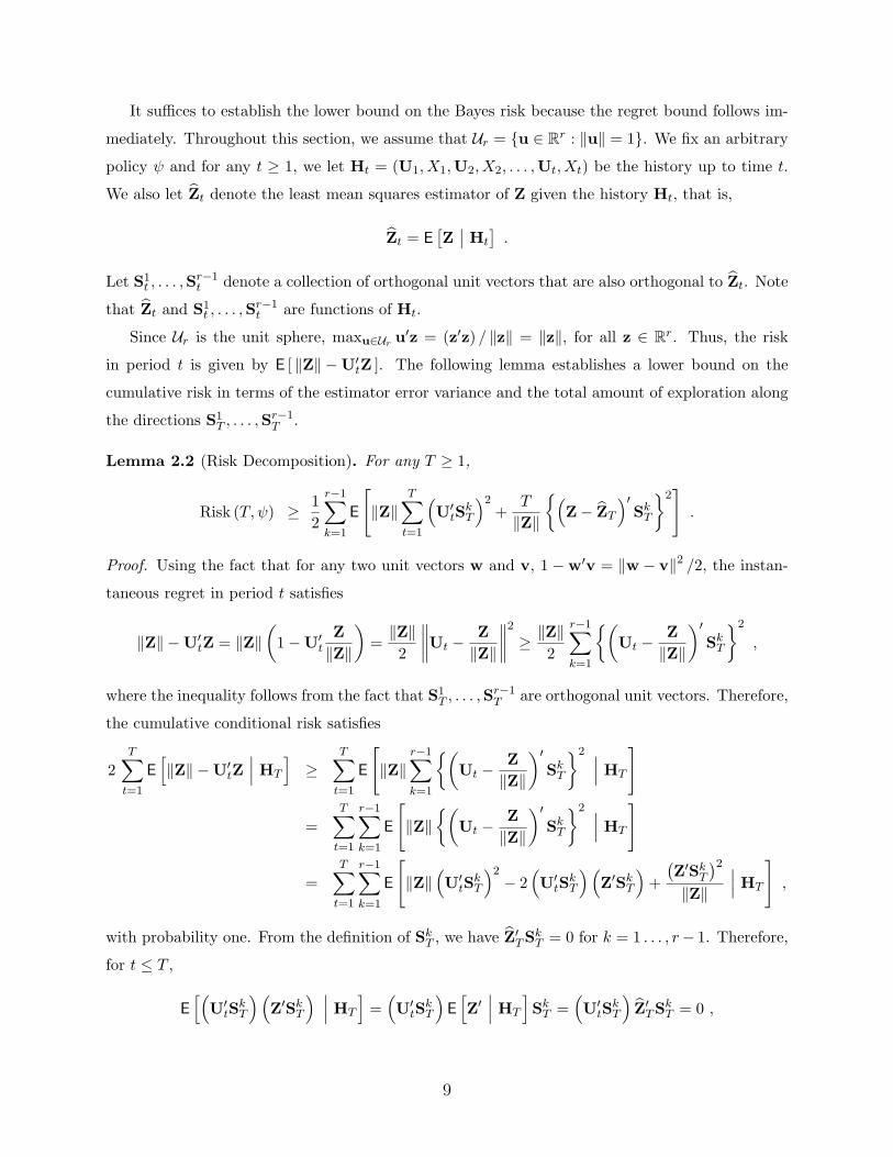
Lemma 2.2 (Risk Decomposition). For any T ≥ 1,

Risk (T, ψ) ≥ 12

r−1∑k=1

E

[‖Z‖

T∑t=1

(U′tS

kT

)2+

T

‖Z‖

(Z− ZT

)′SkT

2].

Proof. Using the fact that for any two unit vectors w and v, 1 −w′v = ‖w − v‖2 /2, the instan-

taneous regret in period t satisfies

‖Z‖ −U′tZ = ‖Z‖(

1−U′tZ‖Z‖

)=‖Z‖

2

∥∥∥∥Ut −Z‖Z‖

∥∥∥∥2

≥ ‖Z‖2

r−1∑k=1

(Ut −

Z‖Z‖

)′SkT

2

,

where the inequality follows from the fact that S1T , . . . ,S

r−1T are orthogonal unit vectors. Therefore,

the cumulative conditional risk satisfies

2T∑t=1

E[‖Z‖ −U′tZ

∣∣∣ HT

]≥

T∑t=1

E

[‖Z‖

r−1∑k=1

(Ut −

Z‖Z‖

)′SkT

2 ∣∣∣ HT

]

=T∑t=1

r−1∑k=1

E

[‖Z‖

(Ut −

Z‖Z‖

)′SkT

2 ∣∣∣ HT

]

=T∑t=1

r−1∑k=1

E

[‖Z‖

(U′tS

kT

)2− 2

(U′tS

kT

)(Z′SkT

)+

(Z′SkT

)2‖Z‖

∣∣∣ HT

],

with probability one. From the definition of SkT , we have Z′TSkT = 0 for k = 1 . . . , r− 1. Therefore,

for t ≤ T ,

E[(

U′tSkT

)(Z′SkT

) ∣∣∣ HT

]=(U′tS

kT

)E[Z′∣∣∣ HT

]SkT =

(U′tS

kT

)Z′TSkT = 0 ,

9

which eliminates the middle term in the summand above. Furthermore, we see that Z′SkT =(Z− ZT

)′SkT for all k. Thus, with probability one,

T∑t=1

E[‖Z‖ −U′tZ

∣∣∣ HT

]≥ 1

2

r−1∑k=1

E

[‖Z‖

T∑t=1

(U′tS

kT

)2+

T

‖Z‖

(Z− ZT

)′SkT

2 ∣∣∣ HT

],

and the desired result follows by taking the expectation of both sides.

Since SkT is orthogonal to ZT , we can interpret∑T

t=1

(U′tS

kT

)2 and(

Z− ZT)′

SkT

2

as the

total amount of exploration over T periods and the squared estimation error, respectively, in the

direction SkT . Thus, Lemma 2.2 tells us that the cumulative risk is bounded below by the sum

of the squared estimation error and the total amount of exploration in the past T periods. This

result suggests an approach for establishing a lower bound on the risk. If the amount of exploration∑Tt=1

(U′tS

kT

)2 is large, then the risk will be large. On the other hand, if the amount of exploration

is small, we expect significant estimation errors, which in turn imply large risk. This intuition

is made precise in Lemma 2.3, which relates the squared estimation error and the amount of

exploration.

Lemma 2.3 (Little Exploration Implies Large Estimation Errors). For any k and T ≥ 1,

E

[(Z− ZT

)′SkT

2 ∣∣∣∣ HT

]≥ 1

r +∑T

t=1

(U′tS

kT

)2 ,

with probability one.

Proof. Let QT = ZT/‖ZT ‖. For any t, we have that Ut =

∑r−1k=1

(U′tS

kT

)SkT + (U′tQT ) QT . Let

V =[S1T S2

T · · · Sr−1T QT

]be an r× r orthonormal matrix whose columns are the vectors S1

T , . . . ,Sr−1T , and QT , respectively.

Then, it is easy to verify thatT∑t=1

UtU′t = VAV′ ,

where A =

Σ c

c′ a

, is an r × r matrix, with a = Q′T(∑T

t=1 UtU′t)

QT , c is an (r − 1)-

dimensional column vector, and where Σ is an (r−1)×(r−1) matrix with Σk` =(SkT)′ (∑T

t=1 UtU′t)

S`T =∑Tt=1

(U′tS

kT

) (U′tS

`T

)for k, ` = 1, . . . , r − 1,

Since Z has a multivariate normal prior distribution with covariance matrix Ir/r, it is a standard

result (use, for example, Corollary E.3.5 in Appendix E in Bertsekas, 1995) that

E

[(Z− ZT

)(Z− ZT

)′ ∣∣∣∣ HT

]=

(r Ir +

T∑t=1

UtU′t

)−1

= V (r Ir + A)−1 V′ .

10

Since SkT is a function of HT and V′SkT = ek, we have, for k ≤ r − 1, that

E

[(Z− ZT

)′SkT

2 ∣∣∣∣ HT

]=

(V′SkT

)′(rIr + A)−1

(V′SkT

)=[(r Ir + A)−1

]kk

≥ 1(r Ir + A)kk

=1

r +∑T

t=1

(U′tS

kT

)2 ,

where the inequality follows from Fiedler’s Inequality (see, for example, Theorem 2.1 in Fiedler

and Ptak, 1997), and the final equality follows from the definition of A.

The next lemma gives a lower bound on the probability that Z is bounded away from the origin.

The proof follows from simple calculations involving normal densities, and the details are given in

Appendix A.1.

Lemma 2.4. For any θ ≤ 1/2 and β > 0, Pr θ ≤ ‖Z‖ ≤ β ≥ 1− 4θ2 − 1β2 .

The last lemma establishes a lower bound on the sum of the total amount of exploration and

the squared estimation error, which is also the minimum cumulative Bayes risk along the direction

SkT by Lemma 2.2.

Lemma 2.5 (Minimum Directional Risk). For k = 1, . . . , r − 1, and T ≥ r2,

E

[‖Z‖

T∑t=1

(U′tS

kT

)2+

T

‖Z‖

(Z− ZT

)′SkT

2]≥ 0.027

√T .

We note that if ‖Z‖ were a constant, rather than a random variable, Lemma 2.5 would follow

immediately. Hence, most of the work in the proof below involves constraining ‖Z‖ to a certain

range [θ, β].

Proof. Consider an arbitrary k, and let Ξ =∑T

t=1

(U′tS

kT

)2, Γ =(

Z− ZT)′

SkT

2

. Our proof

will make use of positive constants θ, β, and η, whose values will be chosen later. Note that

E

[‖Z‖Ξ +

T Γ‖Z‖

∣∣∣ HT

]≥ E

[(‖Z‖Ξ +

T Γ‖Z‖

)1lθ ≤ ‖Z‖ ≤ β1lΞ ≥

√T∣∣∣ HT

]+ E

[(‖Z‖Ξ +

T Γ‖Z‖

)1lθ ≤ ‖Z‖ ≤ β1lΞ <

√T∣∣∣ HT

]≥ θ

√T 1lΞ ≥

√TE

[1lθ ≤ ‖Z‖ ≤ β

∣∣ HT

]+

T

β1lΞ <

√TE

[Γ 1lθ ≤ ‖Z‖ ≤ β

∣∣ HT

],

where we use the fact that Ξ is a function of HT in the final inequality. We will now lower bound

the last term on the right hand side of the above inequality. Let Θ = E[Γ∣∣ HT

]. Since Θ is a

11

function of HT ,

T

β1lΞ <

√TE

[Γ 1lθ ≤ ‖Z‖ ≤ β

∣∣ HT

]≥ T

β1lΞ <

√TE

[Γ 1lθ ≤ ‖Z‖ ≤ β1lΓ ≥ ηΘ

∣∣ HT

]≥ η T

βΘ 1lΞ <

√TE

[1lθ ≤ ‖Z‖ ≤ β1lΓ ≥ ηΘ

∣∣∣ HT

]≥ η

√T

2β1lΞ <

√TE

[1lθ ≤ ‖Z‖ ≤ β1lΓ ≥ ηΘ

∣∣∣ HT

],

where the last inequality follows from Lemma 2.3 which implies that, with probability one,

η T

βΘ 1lΞ <

√T ≥

η T

β· 1r + Ξ

1lΞ <√T ≥

η T

β· 1r +√T

1lΞ <√T ≥

η√T

2β1lΞ <

√T ,

and where the last inequality follows from the fact that T ≥ r2, and thus, 1/(r +√T)≥ 1/(2

√T ).

Putting everything together, we obtain

E

[‖Z‖Ξ +

T Γ‖Z‖

∣∣∣ HT

]≥ θ

√T 1lΞ ≥

√TE

[1lθ ≤ ‖Z‖ ≤ β

∣∣ HT

]+

η√T

2β1lΞ <

√TE

[1lθ ≤ ‖Z‖ ≤ β1lΓ ≥ ηΘ

∣∣∣ HT

],

≥ minθ,

η

2β

√T E

[1lθ ≤ ‖Z‖ ≤ β1lΓ ≥ ηΘ

∣∣∣ HT

],

with probability one. By the Bonferroni Inequality, we have that

E[1lθ ≤ ‖Z‖ ≤ β1lΓ ≥ ηΘ

∣∣ HT

]= Pr

θ ≤ ‖Z‖ ≤ β and Γ ≥ ηΘ

∣∣ HT

≥ Pr

θ ≤ ‖Z‖ ≤ β

∣∣ HT

+ Pr

Γ ≥ ηΘ

∣∣ HT

− 1 ,

with probability one. Conditioned on HT ,(Z− ZT

)′SkT is normally distributed with mean zero

and variance

E

[(Z− ZT

)′SkT

2 ∣∣∣ HT

]= E

[Γ∣∣∣ HT

]= Θ .

Let Φ(·) be the cumulative distribution function of the standard normal random variable, that is,

Φ(x) = 1√2π

∫ x−∞ e

−u2/2 du. Then,

Pr

Γ ≥ ηΘ∣∣ HT

= Pr

∣∣ (Z− ZT)′

SkT∣∣ ≥ √η√Θ

∣∣ HT

= 2 (1− Φ (

√η)) ,

from which it follows that, with probability one,

E[1lθ ≤ ‖Z‖ ≤ β1lΓ ≥ ηΘ

∣∣∣ HT

]≥ Pr

θ ≤ ‖Z‖ ≤ β

∣∣ HT

+ 2 (1− Φ (

√η))− 1 .

Therefore,

E

[‖Z‖Ξ +

T Γ‖Z‖

∣∣∣ HT

]≥ min

θ,

η

2β

[Prθ ≤ ‖Z‖ ≤ β

∣∣∣ HT

+ 2 (1− Φ (

√η))− 1

]√T ,

12

with probability one, which implies that

E

[‖Z‖Ξ +

T Γ‖Z‖

]≥ min

θ,

η

2β

[Pr θ ≤ ‖Z‖ ≤ β+ 2 (1− Φ (

√η))− 1]

√T ,

≥ minθ,

η

2β

[2 (1− Φ (

√η))− 1

β2− 4θ2

] √T ,

where the last inequality follows from Lemma 2.4. Set θ = 0.09, β = 3, and η = 0.5, to obtain

E[‖Z‖Ξ + T Γ

‖Z‖

]≥ 0.027

√T , which is the desired result.

Finally, here is the proof of Theorem 2.1.

Proof. It follows from Lemmas 2.2 and 2.5 that

Risk (T, ψ) ≥ 12

r−1∑k=1

E

[‖Z‖

T∑t=1

(U′tS

kT

)2+

T

‖Z‖

(Z− ZT

)′SkT

2]

≥ r − 12· 0.027

√T ≥ r

4· 0.027

√T ≥ 0.006 r

√T ,

where we have used the fact r ≥ 2, which implies that r − 1 ≥ r/2.

3. Matching Upper Bounds

We have established Ω(r√T)

lower bounds when the set of arms Ur is the unit sphere. We now

prove that a policy that alternates between exploration and exploitation phases yields matching

upper bounds on the regret and risk, and is therefore optimal for this problem. Surprisingly, we

will see that the phase-based policy is effective for a large class of bandit problems, involving a

strongly convex set of arms. We introduce the following assumption on the tails of the error random

variables Wut and on the set of arms Ur, which will remain in effect throughout the rest of paper.

Assumption 1.

(a) There exists a positive constant σ0 such that for any r ≥ 2, u ∈ Ur, t ≥ 1, and x ∈ R, we

have E[exW

ut]≤ ex2σ2

0/2 .

(b) There exist positive constants u and λ0 such that for any r ≥ 2,

maxu∈Ur

‖u‖ ≤ u ,

and the set of arms Ur ⊂ Rr has r linearly independent elements b1, . . . ,br such that

λmin (∑r

k=1 bkb′k) ≥ λ0.

Under Assumption 1(a), the tails of the distribution of the errors Wut decay at least as fast as

for a normal random variable with variance σ20. The first part of Assumption 1(b) ensures that

13

the expected reward of the arms remain bounded as the dimension r increases, while the arms

b1, . . . ,br given in the second part of Assumption 1(b) will be used during the exploration phase

of our policy.

Our policy – which we refer to as the Phased Exploration and Greedy Exploitation

(PEGE) – operates in cycles, and in each cycle, we alternate between exploration and exploitation

phases. During the exploration phase of cycle c, we play the r linearly independent arms from

Assumption 1(b). Using the rewards observed during the exploration phases in the past c cycles,

we compute an ordinary least squares (OLS) estimate Z(c). In the exploitation phase of cycle c,

we use Z(c) as a proxy for Z and compute a greedy decision G(c) ∈ Ur defined by:

G(c) = arg maxv∈Ur

v′Z(c) , (2)

where we break ties arbitrarily. We then play the arm G(c) for an additional c periods to complete

cycle c. Here is a formal description of the policy.

Phased Exploration and Greedy Exploitation (PEGE)

Description: For each cycle c ≥ 1, complete the following two phases.

1. Exploration (r periods): For k = 1, 2, . . . , r, play arm bk ∈ Ur given in Assumption 1(b),

and observe the reward Xbk(c). Compute the OLS estimate Z(c) ∈ Rr, given by

Z(c) =1c

(r∑

k=1

bkb′k

)−1 c∑s=1

r∑k=1

bkXbk(s) = Z +1c

(r∑

k=1

bkb′k

)−1 c∑s=1

r∑k=1

bkWbk(s) ,

where for any k, Xbk(s) and Wbk(s) denote the observed reward and the error random

variable associated with playing arm bk in cycle s. Note that the last equality follows from

Equation (1) defining our model.

2. Exploitation (c periods): Play the greedy arm G(c) = arg maxv∈Ur v′Z(c) for c periods.

Since Ur is compact, for each z ∈ Rr, there is an optimal arm that gives the maximum expected

reward. When this best arm varies smoothly with z, we will show that the T -period regret and

risk under the PEGE policy is bounded above by O(r√T ). More precisely, we say that a set of

arms Ur satisfies the smooth best arm response with parameter J (SBAR(J), for short) condition if

for any nonzero vector z ∈ Rr \0, there is a unique best arm u∗(z) ∈ Ur that gives the maximum

expected reward, and for any two unit vectors z ∈ Rr an y ∈ Rr with ‖z‖ = ‖y‖ = 1, we have

‖u∗(z)− u∗(y)‖ ≤ J ‖z− y‖ .

14

Even though the SBAR condition appears to be an implicit one, it admits a simple interpreta-

tion. According to Corollary 4 of Polovinkin (1996), a compact set Ur satisfies condition SBAR(J)

if and only if it is strongly convex with parameter J , in the sense that the set Ur can be represented

as the intersection of closed balls of radius J . Intuitively, the SBAR condition requires the bound-

ary of Ur to have a curvature that is bounded below by a positive constant. For some examples,

the unit ball satisfies the SBAR(1) condition. Furthermore, according to Theorem 3 of Polovinkin

(1996), an ellipsoid of the form u ∈ Rr : u′Q−1u ≤ 1, where Q is a symmetric positive definite

matrix, satisfies the condition SBAR(λmax(Q)/

√λmin(Q)

).

The main result of this section is stated in the following theorem. The proof is given in Sec-

tion 3.1.

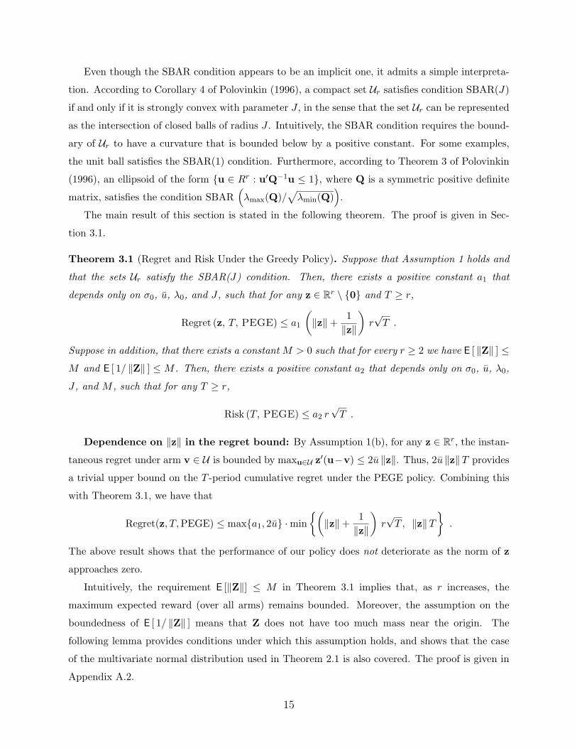
Theorem 3.1 (Regret and Risk Under the Greedy Policy). Suppose that Assumption 1 holds and

that the sets Ur satisfy the SBAR(J) condition. Then, there exists a positive constant a1 that

depends only on σ0, u, λ0, and J , such that for any z ∈ Rr \ 0 and T ≥ r,

Regret (z, T, PEGE) ≤ a1

(‖z‖+

1‖z‖

)r√T .

Suppose in addition, that there exists a constant M > 0 such that for every r ≥ 2 we have E [ ‖Z‖ ] ≤

M and E [ 1/ ‖Z‖ ] ≤ M . Then, there exists a positive constant a2 that depends only on σ0, u, λ0,

J , and M , such that for any T ≥ r,

Risk (T, PEGE) ≤ a2 r√T .

Dependence on ‖z‖ in the regret bound: By Assumption 1(b), for any z ∈ Rr, the instan-

taneous regret under arm v ∈ U is bounded by maxu∈U z′(u−v) ≤ 2u ‖z‖. Thus, 2u ‖z‖T provides

a trivial upper bound on the T -period cumulative regret under the PEGE policy. Combining this

with Theorem 3.1, we have that

Regret(z, T,PEGE) ≤ maxa1, 2u ·min(‖z‖+

1‖z‖

)r√T , ‖z‖T

.

The above result shows that the performance of our policy does not deteriorate as the norm of z

approaches zero.

Intuitively, the requirement E [‖Z‖] ≤ M in Theorem 3.1 implies that, as r increases, the

maximum expected reward (over all arms) remains bounded. Moreover, the assumption on the

boundedness of E [ 1/ ‖Z‖ ] means that Z does not have too much mass near the origin. The

following lemma provides conditions under which this assumption holds, and shows that the case

of the multivariate normal distribution used in Theorem 2.1 is also covered. The proof is given in

Appendix A.2.

15

Lemma 3.2 (Small Mass Near the Origin).

(a) Suppose that there exist constants M0 and ρ ∈ (0, 1] such that for any r ≥ 2, the random

variable ‖Z‖ has a density function g : R+ → R+ such that g(x) ≤ M0xρ for all x ∈ [0, ρ].

Then, E [ 1/ ‖Z‖ ] ≤M , where M depends only on M0 and ρ.

(b) Suppose that for any r ≥ 2, the random vector Z has a multivariate normal distribution with

mean 0 ∈ Rr and covariance matrix Ir/r. Then, E [ ‖Z‖ ] ≤ 1 and E [ 1/ ‖Z‖ ] ≤√π.

The following corollary shows that the example in Section 2 admits tight matching upper bounds

on the regret and risk.

Corollary 3.3 (Matching Upper Bounds). Consider a bandit problem where the set of arms is the

unit sphere in Rr, and where Wut has a standard normal distribution with mean zero and variance

one for all t and u. Then, there exists an absolute constant a3 such that for any z ∈ Rr \ 0 and

T ≥ r,

Regret (z, T,PEGE) ≤ a3

(‖z‖+

1‖z‖

)r√T .

Moreover, if Z has a multivariate normal distribution with mean 0 and covariance matrix Ir/r,

then for all T ≥ r,

Risk (T,PEGE) ≤ a3 r√T .

Proof. Since the set of arms is the unit sphere and the errors are standard normal, Assumption

1 is satisfied with σ0 = u = λ0 = 1. Moreover, as already discussed, the unit sphere satisfies

the SBAR(1) condition. Finally, By Lemma 3.2, the random vector Z satisfies the hypotheses of

Theorem 3.1. The regret and risk bounds then follow immediately.

3.1 Proof of Theorem 3.1

The proof of Theorem 3.1 relies on the following upper bound on the square of the norm difference

between Z(c) and Z.

Lemma 3.4 (Bound on Squared Norm Difference). Under Assumption 1, there exists a positive

constant h1 that depends only on σ0, u, and λ0 such that for any z ∈ Rr and c ≥ 1,

E

[∥∥∥Z(c)− z∥∥∥2 ∣∣∣ Z = z

]≤ h1 r

c.

Proof. Recall from the definition of the PEGE policy that the estimate Z(c) at the end of the

exploration phase of cycle c is given by

Z(c) = Z +1c

(r∑

k=1

bkb′k

)−1 c∑s=1

r∑k=1

bkWbk(s) = Z +1c

c∑s=1

B V(s) ,

16

where B = (∑r

k=1 bkb′k)−1 and V(s) =

∑rk=1 bkWbk(s). Note that the mean-zero random vari-

ables Wbk(s) are independent of each other and their variance is bounded by some constant γ0

that depends only on σ0. Then, it follows from Assumption 1 that

E

[∥∥∥Z(c)− z∥∥∥2 ∣∣∣ Z = z

]=

1c2

c∑s=1

E[V(s)′B2V(s)

]=

1c2

c∑s=1

r∑k=1

E

[(Wbk(s)

)2]

b′kB2bk

≤ γ0

c

r∑k=1

b′kB2bk ≤

γ0

c

r∑k=1

λmax

(B2)‖bk‖2 ≤

γ0 u2 r

λ20 c

,

which is the desired result.

The next lemma gives an upper bound on the difference between two normalized vectors in

terms of the difference of the original vectors.

Lemma 3.5 (Difference Between Normalized Vectors). For any z, w ∈ Rr, not both equal to zero,∥∥∥∥ w‖w‖

− z‖z‖

∥∥∥∥ ≤ 2 ‖w − z‖max ‖z‖ , ‖w‖

,

where we define 0/ ‖0‖ to be some fixed unit vector.

Proof. The inequality is easily seen to hold if either w = 0 or z = 0. So, assume that both w and

z are nonzero. Using the triangle inequality and the fact that∣∣ ‖w‖ − ‖z‖ ∣∣ ≤ ‖w − z‖, we have

that∥∥∥∥ w‖w‖

− z‖z‖

∥∥∥∥ ≤ ∥∥∥∥ w‖w‖

− z‖w‖

∥∥∥∥+∥∥∥∥ z‖w‖

− z‖z‖

∥∥∥∥ =‖w − z‖‖w‖

+ ‖z‖∣∣∣∣ 1‖w‖

− 1‖z‖

∣∣∣∣ ≤ 2 ‖w − z‖‖w‖

.

By symmetry, we also have∥∥∥ w‖w‖ −

z‖z‖

∥∥∥ ≤ 2‖w−z‖‖z‖ , which gives the desired result.

The following lemma gives an upper bound on the expected instantaneous regret under the

greedy decision G(c) during the exploitation phase of cycle c.

Lemma 3.6 (Regret Under the Greedy Decision). Suppose that Assumption 1 holds and the sets

Ur satisfy the SBAR(J) condition. Then, there exists a positive constant h2 that depends only on

σ0, u, λ0, and J , such that for any z ∈ Rr and c ≥ 1,

E

[maxu∈Ur

z′ (u−G(c))∣∣∣ Z = z

]≤ r h2

c ‖z‖,

Proof. The result is trivially true when z = 0. So, let us fix some z ∈ Rr \ 0. By comparing the

greedy decision G(c) with the best arm u∗(z), we see that the instantaneous regret satisfies

z′ (u∗ (z)−G(c)) =(z− Z(c)

)′u∗ (z) + (u∗ (z)−G(c))′ Z(c) +

(Z(c)− z

)′G(c)

≤(z− Z(c)

)′u∗ (z) +

(Z(c)− z

)′G(c)

=(Z(c)− z

)′(G(c)− u∗ (z)) =

(Z(c)− z

)′ (u∗(Z(c)

)− u∗ (z)

),

17

where the inequality follows from the definition of the greedy decision in Equation (2), and the

final equality follows from the fact that G(c) = u∗(Z(c)

). As a convention, we define 0/ ‖0‖ to

some fixed unit vector and set u∗(0) = u∗(0/ ‖0‖).

It then follows from the Cauchy-Schwarz Inequality that, with probability one,

z′ (u∗(z)−G(c)) ≤∥∥∥Z(c)− z

∥∥∥∥∥∥u∗ (Z(c))− u∗(z)

∥∥∥=

∥∥∥Z(c)− z∥∥∥∥∥∥∥∥u∗

(Z(c)

‖Z(c)‖

)− u∗

(z‖z‖

)∥∥∥∥∥≤ J

∥∥∥Z(c)− z∥∥∥∥∥∥∥∥ Z(c)

‖Z(c)‖− z‖z‖

∥∥∥∥∥ ≤ 2J∥∥∥Z(c)− z

∥∥∥2

‖z‖,

where the equality follows from the fact that u∗(z) = u∗(λz) for all λ > 0. The second inequality

follows from condition SBAR(J), and the final inequality follows from Lemma 3.5. The desired

result follows by taking conditional expectations, given Z = z, and applying Lemma 3.4.

We can now complete the proof of Theorem 3.1, by adding the regret over the differnt times

and cycles. By Assumption 1 and the Cauchy-Schwarz Inequality, the instantaneous regret from

playing any arm u ∈ Ur is bounded above by maxv∈Ur z′ (v − u) ≤ 2 u ‖z‖. Consider an arbitrary

cycle c. Then, the total regret incurred during the exploration phase (with r periods) in this

cycle is bounded above by 2 u r ‖z‖. During the exploitation phase of cycle c, we always play

the greedy arm G(c). The expected instantaneous regret in each period during the exploitation

phase is bounded above by rh2/c ‖z‖. So, the total regret during cycle c is bounded above by

2 u r ‖z‖+ h2 r/ ‖z‖. Summing over K cycles, we obtain

Regret

(z, rK +

K∑c=1

c, PEGE

)≤ h3 r ‖z‖K + h4

K∑c=1

r

‖z‖,

for some positive constants h3 and h4 that depend only on σ0, u, λ0, and J .

Consider an arbitrary time period T ≥ r and z ∈ Rr. Let K0 =⌈√

2T⌉. Note that the total

time periods after K0 cycles is at least T because rK0 +∑K0

c=1 c ≥∑K0

c=1 c = K0(K0+1)2 ≥ K2

02 ≥ T .

Since the cumulative regret is nondecreasing over time, it follows that

Regret (z, T,PEGE) ≤ Regret

(z, rK0 +

K0∑c=1

c, PEGE

)

≤ h3 r ‖z‖K0 + h4rK0

‖z‖≤ 3 maxh3, h4

(‖z‖+

1‖z‖

)r√T ,

where the final inequality follows because K0 =⌈√

2T⌉≤ 3√T . The risk bound follows by taking

expectations and using the assumption on the boundedness of E[ ‖Z‖ ] and E[ 1/ ‖Z‖ ].

18

4. A Policy for General Bandits

We have shown that when a bandit has a smooth best arm response, the PEGE policy achieves

optimal O(r√T ) regret and Bayes risk. The general idea is that when the estimation error is small,

the instantaneous regret of the greedy decision based on our estimate Z(c) can be of the same order

as ‖Z− Z(c)‖. However, under the smoothness assumption, this upper bound on the instantaneous

regret is improved to O(‖Z− Z(c)‖2

), as shown in the proof of Lemma 3.6, and this enables us

to separate exploration from exploitation.

However, if the number of arms is finite or if the collection of arms is an arbitrary compact

set, then the PEGE policy may not be effective. This is because a small estimation error may

have a disproportionately large effect on the arm chosen by a greedy policy, leading to a large

instantaneous regret. In this section, we discuss a policy – which we refer to as the Uncertainty

Ellipsoid (UE) policy – that can be applied to any bandit problem, at the price of slightly higher

regret and Bayes risk. In contrast to the PEGE policy, the UE policy combines active exploration

and exploitation in every period.

As discussed in the introduction, the UE policy is closely related to the algorithms described

in Auer (2002) and Dani et al. (2008a), but also has the “anytime” property (the policy does not

require prior knowledge of the time horizon T ), and also allows the random vector Z and the errors

Wut to be unbounded. For the sake of completeness, we give a detailed description of our policy and

state the regret and risk bounds that we obtain. The reader can find the proofs of these bounds in

Appendix B.

To facilitate exposition, we introduce a constant that will appear in the description of the policy,

namely,

κ0 = 2

√1 + log

(1 +

36 u2

λ0

), (3)

where the parameters u and λ0 are given in Assumption 1. The UE policy maintains, at each time

period t, the following two pieces of information.

1. The ordinary least squares (OLS) estimate defined as follows: if U1, . . . ,Ut are the arms

chosen during the first t periods, then the OLS estimate Zt is given by4:

Ct =

(t∑

s=1

UsU′s

)−1

, Mt =t∑

s=1

UsWs , and Zt = Ct

t∑s=1

UsXs = Z + CtMt . (4)

4Let us note that we are abusing notation here. Throughout this section Zt stands for the OLS estimate, which is

different from the least mean squares estimator E[Z∣∣ Ht

]introduced in Section 2.

19

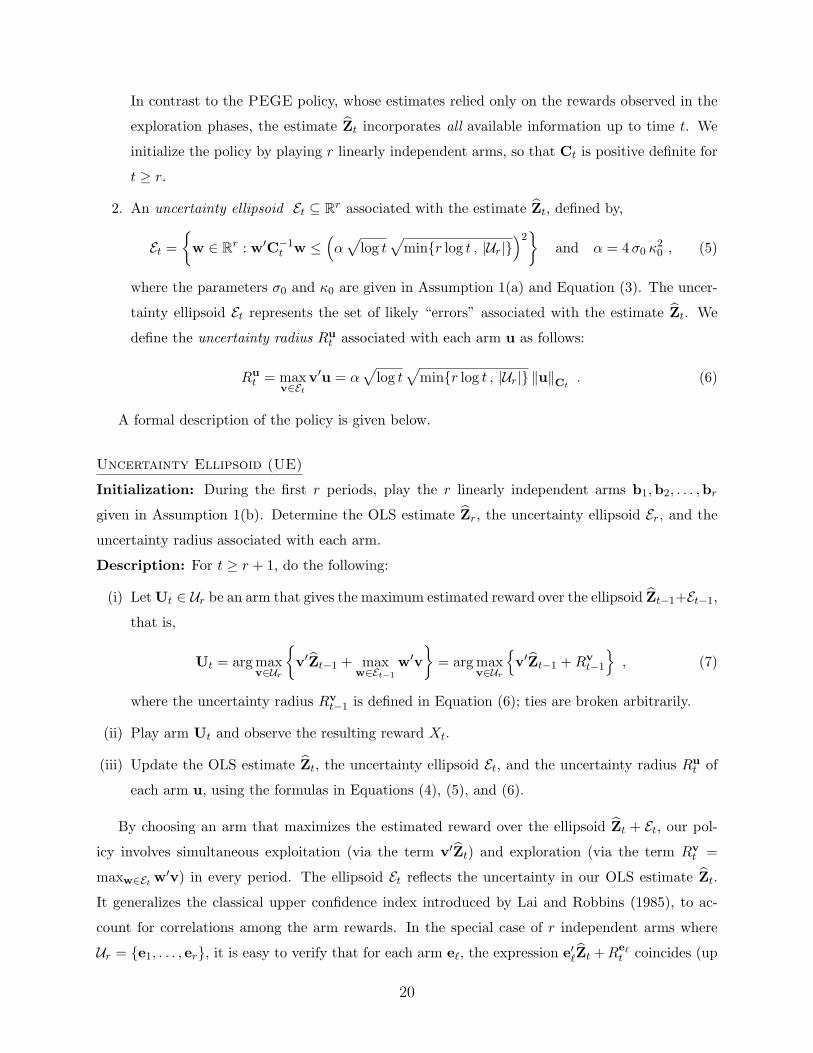
In contrast to the PEGE policy, whose estimates relied only on the rewards observed in the

exploration phases, the estimate Zt incorporates all available information up to time t. We

initialize the policy by playing r linearly independent arms, so that Ct is positive definite for

t ≥ r.

2. An uncertainty ellipsoid Et ⊆ Rr associated with the estimate Zt, defined by,

Et =

w ∈ Rr : w′C−1t w ≤

(α√

log t√

minr log t , |Ur|)2

and α = 4σ0 κ20 , (5)

where the parameters σ0 and κ0 are given in Assumption 1(a) and Equation (3). The uncer-

tainty ellipsoid Et represents the set of likely “errors” associated with the estimate Zt. We

define the uncertainty radius Rut associated with each arm u as follows:

Rut = max

v∈Etv′u = α

√log t

√minr log t , |Ur| ‖u‖Ct

. (6)

A formal description of the policy is given below.

Uncertainty Ellipsoid (UE)

Initialization: During the first r periods, play the r linearly independent arms b1,b2, . . . ,br

given in Assumption 1(b). Determine the OLS estimate Zr, the uncertainty ellipsoid Er, and the

uncertainty radius associated with each arm.

Description: For t ≥ r + 1, do the following:

(i) Let Ut ∈ Ur be an arm that gives the maximum estimated reward over the ellipsoid Zt−1+Et−1,

that is,

Ut = arg maxv∈Ur

v′Zt−1 + max

w∈Et−1

w′v

= arg maxv∈Ur

v′Zt−1 +Rv

t−1

, (7)

where the uncertainty radius Rvt−1 is defined in Equation (6); ties are broken arbitrarily.

(ii) Play arm Ut and observe the resulting reward Xt.

(iii) Update the OLS estimate Zt, the uncertainty ellipsoid Et, and the uncertainty radius Rut of

each arm u, using the formulas in Equations (4), (5), and (6).

By choosing an arm that maximizes the estimated reward over the ellipsoid Zt + Et, our pol-

icy involves simultaneous exploitation (via the term v′Zt) and exploration (via the term Rvt =

maxw∈Et w′v) in every period. The ellipsoid Et reflects the uncertainty in our OLS estimate Zt.

It generalizes the classical upper confidence index introduced by Lai and Robbins (1985), to ac-

count for correlations among the arm rewards. In the special case of r independent arms where

Ur = e1, . . . , er, it is easy to verify that for each arm e`, the expression e′`Zt +Re`t coincides (up

20

to a scaling constant) with the upper confidence bound used by Auer et al. (2002). Our definition

of the uncertainty radius involves an extra factor of√

minr log t, |Ur|, in order to handle the case

where the arms are not standard unit vectors, and the rewards are correlated.

The main results of this section are given in the following two theorems. The first theorem

establishes upper bounds on the regret and risk when the set of arms is an arbitrary compact set.

This result shows that the UE policy is nearly optimal, admitting upper bounds that are within a

logarithmic factor of the Ω(r√T ) lower bounds given in Theorem 2.1. Although the proof of this

theorem makes use of somewhat different (and novel) large deviation inequalities for adaptive least

squares estimators, the argument shares similarities with the proofs given in Dani et al. (2008a),

and we omit the details. The reader can find a complete proof in Appendix B.2.

Theorem 4.1 (Bounds for General Compact Sets of Arms). Under Assumption 1, there exist

positive constants a4 and a5 that depend only on the parameters σ0, u, and λ0, such that for all

T ≥ r + 1 and z ∈ Rr,

Regret (z, T,UE) ≤ a4r ‖z‖+ a5 r√T log3/2 T ,

and

Risk (T,UE) ≤ a4r E [‖Z‖] + a5 r√T log3/2 T .

For any arm u ∈ Ur and z ∈ Rr, let ∆u (z) denote the difference between the maximum expected

reward and the expected reward of arm u when Z = z, that is,

∆u (z) = maxv∈Ur

v′z− u′z .

When the number of arms is finite, it turns out that we can obtain bounds on regret and risk that

scale more gracefully over time, growing as log T and log2 T , respectively. This result is stated in

Theorem 4.2, which shows that, for a fixed set of arms, the UE policy is asymptotically optimal

as a function time, within a constant factor of the lower bounds established by Lai and Robbins

(1985) and Lai (1987).

Theorem 4.2 (Bounds for Finitely Many Arms). Under Assumption 1, there exist positive con-

stants a6 and a7 that depend only on the parameters σ0, u, and λ0 such that for all T ≥ r+ 1 and

z ∈ Rr,

Regret (z, T,UE) ≤ a6 |Ur| ‖z‖+ a7 |Ur|∑u∈Ur

min

log T∆u (z)

, T∆u(z).

Moreover, suppose that there exists a positive constant M0 such that, for all arms u, the distribution

of the random variable ∆u (Z) is described by a point mass at 0, and a density function that is

21

bounded above by M0 on R+. Then, there exist positive constants a8 and a9 that depend only on

the parameters σ0, u, λ0, and M0, such that for all T ≥ r + 1,

Risk (T,UE) ≤ a8 |Ur| E [‖Z‖] + a9 |Ur|2 log2 T .

Proof. For any arm u ∈ Ur and z ∈ Rr, let the random variable Nu(z, T ) denote the total number

of times that the arm u is chosen during periods 1 through T , given that Z = z. Using an argument

similar to the one in Auer et al. (2002), we can show that

E [Nu(z, T ) | Z = z] ≤ 6 +4α2 |Ur| log T

(∆u (z))2 .

The reader can find a proof of this result in Appendix B.3.

The regret bound in Theorem 4.2 then follows immediately from the above upper bound and

the fact that Nu(z, T ) ≤ T with probability one, because

Regret (z, T,UE) =∑u∈Ur

∆u (z) E [Nu(z, T ) | Z = z] ≤∑u∈Ur

∆u (z) min

6 +4α2 |Ur| log T

(∆u (z))2 , T

≤ 6

∑u∈Ur

∆u (z) + max4α2, 1 |Ur|∑u∈Ur

min

log T∆u (z)

, T∆u (z),

and the desired result follows from the fact that ∆u(z) = maxv∈Ur (v − u)′ z ≤ 2u ‖z‖, by the

Cauchy-Schwarz Inequality.

We will now establish an upper bound on the Bayes risk. From the regret bound, it suffices to

show that for any u ∈ Ur,

E

[min

log T

∆u (Z), T∆u (Z)

]≤ (M0 + 1) log T +M0 log2 T .

Let qu(·) denote the density function associated with the random variable ∆u (Z). Then,

E

[min

log T

∆u (Z), T∆u (Z)

]=

∫ qlog TT

0min

log Tx

, Tx

qu(x)dx

+∫ 1q

log TT

min

log Tx

, Tx

qu(x)dx+

∫ ∞1

min

log Tx

, Tx

qu(x)dx .

We will now proceed to bound each of the three terms on the right hand side of the above

equality. Having assumed that qu(·) ≤M0, the first term satisfies∫ √(log T )/T

0min

log Tx

, Tx

qu(x)dx ≤M0

∫ √(log T )/T

0Tx dx = M0T

x2

2

∣∣∣√(log T )/T

0≤M0 log T .

For the second term, note that∫ 1

√(log T )/T

min

log Tx

, Tx

qu(x)dx ≤ M0

∫ 1

√(log T )/T

log Tx

dx = M0 log T ·(

log x∣∣∣1√

(log T )/T

)= M0 (log T ) · log T − log log T

2≤M0 log2 T ,

22

where the last inequality follows from the fact that log T − log log T ≤ 2 log T for all T ≥ 2. To

evaluate the last term, note that log Tx ≤ log T for all x ≥ 1, and thus,

∫∞1 min

log Tx , Tx

qu(x)dx ≤

log T∫∞

1 qu(x) ≤ log T . Putting everything together, we have that E[min

log T

∆u(Z) , T∆u (Z)]≤

(M0 + 1) log T +M0 log2 T , which is the desired result.

We conclude this section by giving an example of a random vector Z that satisfies the condition

in Theorem 4.2. A similar example also appears in Example 2 of Lai (1987).

Example 4.3 (IID Random Variables). Suppose Ur = e1, . . . , er and Z = (Z1, . . . , Zr), where

the random variables Zk are independent and identically distributed with a common cumula-

tive distribution function F and a density function f : R → R which is bounded above by M .

Then, for each k, the random variable ∆ek (Z) is given by ∆ek (Z) = (maxj=1,...,r Zj) − Zk =

max 0 , maxj 6=k Zj − Zk . It is easy to verify that ∆ek (Z) has a point mass at 0 and a con-

tinuous density function qk(·) on R+ given by: for any x > 0,

qk(x) = (r − 1)∫F (zk + x)r−2 f(zk + x)f(zk)dzk ≤ (r − 1)M .

4.1 Regret Bounds for Polyhedral Sets of Arms

In this section, we focus on the regret profiles when the set of arms Ur is a polyhedral set. Let

E(Ur) denote the set of extreme points of Ur. From a standard result in linear programming, for

all z ∈ Rr,

maxu∈Ur

u′z = maxu ∈ E(Ur)

u′z .

Since a polyhedral set has a finite number of extreme points (|E(Ur)| < ∞), the parameterized

bandit problem can be reduced to the standard multi-armed bandit problem, where each arm

corresponds to an extreme point of Ur. We can thus apply the algorithm of Lai and Robbins (1985)

and obtain the following upper bound on the T -period cumulative regret for polyhedra

Regret (z, T,Lai’s Algorithm) = O

(|E(Ur)| · log T

min ∆u(z) : ∆u(z) > 0

), (8)

where the denominator corresponds to the difference between the expected reward of the optimal

and the second best extreme points. The algorithm of Lai and Robbins (1985) is effective only when

the polyhedral set Ur has a small number of extreme points, as shown by the following examples.

Example 4.4 (Simplex). Suppose Ur = u ∈ Rr :∑r

i=1 |ui| ≤ 1 is an r-dimensional unit simplex.

Then, Ur has 2r extreme points, and Equation (8) gives an O(r log T ) upper bound on the regret.

23

Example 4.5 (Linear Constraints). Suppose that Ur = u ∈ Rr : Au ≤ b and u ≥ 0, where A

is a p × r matrix with p ≤ r. It follows from the standard linear programming theory that

every extreme point is a basic feasible solution, which has at most p nonzero coordinates (see, for

example, Bertsimas and Tsitsiklis, 1997). Thus, the number of extreme points is bounded above

by(r+pp

)= O((2r)p), and Equation (8) gives an O((2r)p log T ) upper bound on the regret.

In general, the number of extreme points of a polyhedron can be very large, rendering the

bandit algorithm of Lai and Robbins (1985) ineffective; consider, for example, the r-dimensional

cube Ur = u ∈ Rr : |ui| ≤ 1 for all i, which has 2r extreme points. Moreover, we cannot apply

the results and algorithms from Section 3 to the convex hull of Ur. This is because the convex

hull of a polyhedron is not strongly convex (it cannot be written as an intersection of Euclidean

balls), and thus, it does not satisfy the required SBAR(·) condition in Theorem 3.1. The UE policy

in the previous section gives O(r√T log3/2 T ) regret and risk upper bounds. However, finding an

algorithm specifically for polyhedral sets that yields an O(r√T ) regret upper bound (without an

additional logarithmic factor) remains an open question.

5. Conclusion

We analyzed a class of multiarmed bandit problems where the expected reward of each arm depends

linearly on an unobserved random vector Z ∈ Rr, with r ≥ 2. Our model allows for correlations

among the rewards of different arms. When we have a smooth best arm response, we showed that

a policy that alternates between exploration and exploitation is optimal. For a general bandit, we

proposed a near-optimal policy that performs active exploration in every period. For finitely many

arms, our policy achieves asymptotically optimal regret and risk as a function of time, but scales

with the square of the number of arms. Improving the dependence on the number of arms remains

an open question. It would also be interesting to study more general correlation structures. Our

formulation assumes that the vector of expected rewards lies in an r-dimensional subspace spanned

by a known set of basis functions that describe the characteristics of the arms. Extending our work

to a setting where the basis functions are unknown has the potential to broaden the applicability

of our model.

Acknowledgement

The authors would like to thank Adrian Lewis and Mike Todd for helpful and stimulating discussions

on the structure of positive definite matrices and the eigenvalues associated with least squares

estimators, Gena Samorodnitsky for sharing his deep insights on the application of large deviation

theory to this problem, Adam Mersereau for his contributions to the problem formulation, and

24

Assaf Zeevi for helpful suggestions and discussions during the first author’s visit to Columbia

Graduate School of Business. We also want to thank the Associate Editor and the referee for

their helpful comments and suggestions on the paper. This research is supported in part by the

National Science Foundation through grants DMS-0732196, ECCS-0701623, CMMI-0856063, and

CMMI-0855928.

References

Abe, N., and P. M. Long. 1999. Associative reinforcement learning using linear probabilistic concepts. In Proceedings

of the 16th International Conference on Machine Learning, 3–11. San Francisco, CA: Morgan Kaufman.

Agrawal, R. 1995. Sample mean based index policies with O(log n) regret for the multi-armed bandit problem.

Advances in Applied Probability 27 (4): 1054–1078.

Agrawal, R., D. Teneketzis, and V. Anantharam. 1989. Asymptotically efficient adaptive allocation schemes for

controlled I.I.D. processes: finite parameter space. IEEE Transactions on Automatic Control 34 (3): 258–267.

Auer, P. 2002. Using confidence bounds for exploitation-exploration trade-offs. Journal of Machine Learning Re-

search 3:397–422.

Auer, P., N. Cesa-Bianchi, and P. Fischer. 2002. Finite-time analysis of the multiarmed bandit problem. Machine

Learning 47 (2): 235–256.

Berry, D., and B. Fristedt. 1985. Bandit Problems: Sequential Allocation of Experiments. London: Chapman and

Hall.

Bertsekas, D. 1995. Dynamic Programming and Optimal Control, Volume 1. Belmont, MA: Athena Scientific.

Bertsekas, D., and J. N. Tsitsiklis. 1996. Neuro-Dynamic Programming. Belmont, MA: Athena Scientific.

Bertsimas, D., and J. N. Tsitsiklis. 1997. Introduction to Linear Optimization. Belmont, MA: Athena Scientific.

Bhatia, R. 2007. Positive Definite Matrices. Princeton, NJ: Princeton University Press.

Blum, J. R. 1954. Multidimensional Stochastic Approximation Methods. Annals of Mathematical Statistics 25 (4):

737–744.

Cicek, D., M. Broadie, and A. Zeevi. 2009. General bounds and finite-time performance improvement for the Kiefer-

Wolfowitz stochastic approximation algorithm. Working paper. Columbia Graduate School of Business.

Dani, V., T. P. Hayes, and S. M. Kakade. 2008a. Stochastic linear optimization under bandit feedback. In Proceedings

of the 21th Annual Conference on Learning Theory (COLT 2008), 355–366.

Dani, V., T. P. Hayes, and S. M. Kakade. December 2008b. Stochastic linear optimization under bandit feedback.

Working Paper. Available at http://ttic.uchicago.edu/~sham/papers/ml/bandit_linear_long.pdf.

De la Pena, V. H., M. J. Klass, and T. L. Lai. 2004. Self-normalized processes: exponential inequalities, moment

bounds and iterated logarithm laws. Annals of Probability 32 (3A): 1902–1933.

Dudley, R. M. 1999. Uniform Central Limit Theorems. Cambridge: Cambridge University Press.

Feldman, D. 1962. Contributions to the “two-armed bandit” problem. Annals of Mathematical Statistics 33 (3):

847–856.

25

Fiedler, M., and V. Ptak. 1997. A new positive definite geometric mean of two positive defintie matrices. Linear

Algebra and Its Applications 251 (1): 1–20.

Ginebra, J., and M. K. Clayton. 1995. Response surface bandits. Journal of the Royal Statistical Society. Series B

(Methodological) 57 (4): 771–784.

Goldenshluger, A., and A. Zeevi. 2007. Performance limitations in bandit problems with side observations. Working

paper.

Goldenshluger, A., and A. Zeevi. 2008. Woodroofe’s one-armed bandit problem revisited. Working paper.

Keener, R. 1985. Further contributions to the “two-armed bandit” problem. Annals of Statistics 13 (1): 418–422.

Kiefer, J., and J. Wolfowitz. 1952. Stochastic estimation of the maximum of a regression function. Annals of

Mathematical Statistics 23 (3): 462–466.

Lai, T. 2003. Stochastic Approximation (Invited Paper). The Annals of Statistics 31 (2): 391–406.

Lai, T. L. 1987. Adaptive treatment allocation and the multi-armed bandit problem. Annals of Statistics 15 (3):

1091–1114.

Lai, T. L., and H. Robbins. 1985. Asymptotically efficient adaptive allocation rules. Advances in Applied Mathemat-

ics 6 (1): 4–22.

Mersereau, A. J., P. Rusmevichientong, and J. N. Tsitsiklis. 2008. A structured multiarmed bandit problem and the

greedy policy. Working paper.

Pandey, S., D. Chakrabarti, and D. Agrawal. 2007. Multi-armed bandit problems with dependent arms. In Proceedings

of the 24th International Conference on Machine Learning, 721–728.

Polovinkin, E. S. 1996. Strongly convex analysis. Sbornik: Mathematics 187 (2): 259–286.

Pressman, E. L., and I. N. Sonin. 1990. Sequential Control With Incomplete Information. London: Academic Press.

Robbins, H. 1952. Some aspects of the sequential design of experiments. Bulletin of the American Mathematical

Society 58 (5): 527–535.

Robbins, H., and S. Monro. 1951. A stochastic approximation method. Annals of Mathematical Statistics 22 (3):

400–407s.

Sherman, J., and W. J. Morrison. 1950. Adjustment of an inverse matrix corresponding to a change in one element

of a given matrix. Annals of Mathematical Statistics 21 (1): 124–127.

Thompson, W. R. 1933. On the likelihood that one unknown probability exceeds another in view of the evidence of

two samples. Biometrika 25 (3): 285–294.

Wang, C.-C., S. R. Kulkarni, and H. V. Poor. 2005a. Arbitrary side observations in bandit problems. Advances in

Applied Mathematics 34 (4): 903–938.

Wang, C.-C., S. R. Kulkarni, and H. V. Poor. 2005b. Bandit problems with side observations. IEEE Transactions

on Automatic Control 50 (3): 338–355.

A. Properties of Normal Vectors

In this section, we prove that if Z has a multivariate normal distribution with mean 0 ∈ Rr and

covariance matrix Ir/r, then Z has the properties described in Lemmas 2.4 and 3.2.

26

A.1 Proof of Lemma 2.4

We want to establish a lower bound on Pr θ ≤ ‖Z‖ ≤ β. Let Y = (Y1, . . . , Yr) denote the

standard multivariate normal random vector with mean 0 and identity covariance matrix Ir. By

our hypothesis, Z has the same distribution as Y/√r, which implies that

Pr θ ≤ ‖Z‖ ≤ β = Prθ√r ≤ ‖Y‖ ≤ β

√r

= 1− Pr‖Y‖2 < θ2r

− Pr

‖Y‖2 > β2r

.

By definition, ‖Y‖2 = Y 21 + · · · + Y 2

r has a chi-square distribution with r degrees of freedom. By

the Markov Inequality, Pr‖Y‖2 > β2r

≤ E

[‖Y‖2

]/(β2r) = 1/β2. We will now establish an

upper bound on Pr‖Y‖2 < θ2r

. Note that, for any λ > 0,

Pr‖Y‖2 < θ2r

= Pr

e−λ

Prk=1 Y

2k > e−λθ

2r≤ eλθ2r · E

[r∏

k=1

e−λY2k

]=

(eλθ

2

√1 + 2λ

)r,

where last equality follows from the fact that Y1, . . . , Yr are independent standard normal random

variables and thus, E[e−λY

2k

]= 1/

√1 + 2λ for λ > 0. Set λ = 1/θ2, and use the facts θ ≤ 1/2 ≤

√2/e and r ≥ 2, to obtain

Pr‖Y‖2 < θ2r

≤(

eθ√2 + θ2

)r≤(eθ√

2

)r≤(eθ√

2

)2

=e2θ2

2≤ 4θ2 ,

which implies that Pr θ ≤ ‖Z‖ ≤ β ≥ 1− 1β2 − 4θ2, which is the desired result.

A.2 Proof of Lemma 3.2

For part (a) of the lemma, we have

E [ 1/ ‖Z‖ ] =∫ ∞

0

1xg(x) dx ≤ M0

∫ ρ

0xρ−1 dx+

1ρ

∫ ∞ρ

g(x) dx ≤ M0ρρ

ρ+

1ρ.

For the proof of part (b), let Y = (Y1, . . . , Yr) be a standard multivariate normal random vector

with mean 0 and identity covariance matrix, Ir. Then, Z has the same distribution as Y/√r. Note

that ‖Y‖2 has a chi-square distribution with r degrees of freedom. Thus,

E[ ‖Z‖ ] =1√rE[ ‖Y‖ ] ≤ 1√

r

√E[ ‖Y‖2 ] =

1√r

√r = 1 .

We will now establish an upper bound on E[ 1/ ‖Z‖ ] =√r E[ 1/ ‖Y‖ ]. For r = 2, since ‖Y‖

has a chi distribution with two degrees of freedom, we have that

E[ 1/ ‖Z‖ ] =√

2∫ ∞

0

1x· xe−x2/2 dx =

√2∫ ∞

0e−x

2/2 dx =√π .

Consider the case where r ≥ 3. Then,

E[ 1/ ‖Z‖ ] =√r E[ 1/ ‖Y‖ ] ≤

√r

√E[ 1/ ‖Y‖2 ] .

27

Using the formula for the density of the chi-square distribution, we have

E[ 1/ ‖Y‖2 ] =∫ ∞

0

1x· 1

2r/2Γ(r/2)x(r/2)−1e−x/2 dx

=2(r/2)−1

2r/2· Γ((r/2)− 1)

Γ(r/2)·∫ ∞

0

12(r−2)/2Γ((r − 2)/2)

x((r−2)/2)−1e−x/2 dx

=1

2((r/2)− 1)=

1r − 2

≤ 3r,

where the third equality follows from the fact that Γ(r/2) = ((r/2)− 1) ·Γ((r/2)−1) for r ≥ 3 and

the integrand is the density function of the chi-square distribution with r−2 degrees of freedom and

evaluates to 1. The last inequality follows because r ≥ 3. Thus, we have E[ 1/ ‖Z‖ ] ≤√

3 ≤√π,

which is the desired result.

28

B. Proof of Theorems 4.1 and 4.2

In the next section, we establish large deviation inequalities for adaptive least squares estimators

(with unbounded error random variables), which will be used in the proof of Theorems 4.1 and 4.2,

given in Sections B.2 and B.3, respectively.

B.1 Large Deviation Inequalities

The first result extend the standard Chernoff Inequality to our setting involving uncertainty ellip-

soids when we have finitely many arms.

Theorem B.1 (Chernoff Inequality for Uncertainty Ellipsoids with Finitely Many Arms). Under

Assumption 1, for any t ≥ r, x ∈ Rr, z ∈ Rr, and ζ > 0,

Pr

x′(Zt − z

)> ζ σ0 ‖x‖Ct

∣∣ Z = z≤ t5|Ur|e−ζ

2/2,

and

Pr

(Ut+1 − x)′(Zt − z

)> ζ σ0 ‖Ut+1 − x‖Ct

∣∣ Z = z≤ t5|Ur|e−ζ

2/2 .

Proof. We will only prove the second inequality because the proof of the first one follows the same

argument. If the sequence of arms U1,U2, . . . is deterministic (and thus, the matrix Ct is also

deterministic), then

(Ut+1 − x)′(Zt − z

)‖Ut+1 − x‖Ct

=t∑

s=1

(Ut+1 − x)′CtUs

‖Ut+1 − x‖Ct

Ws

andt∑

s=1

((Ut+1 − x)′CtUs

‖Ut+1 − x‖Ct

)2

=(Ut+1 − x)′Ct

(∑ts=1 UsU′s

)Ct (Ut+1 − x)

(Ut+1 − x)′Ct (Ut+1 − x)= 1 .

The classical Chernoff Inequality for the sum of independent random variables (see, for example,

Chapter 1 in Dudley, 1999) then yields

Pr

(Ut+1 − x)′(Zt − z

)> ζ σ0 ‖Ut+1 − x‖Ct

∣∣ Z = z

≤ exp

− ζ2σ2

0

2σ20

∑ts=1

((Ut+1 − x)′CtUs

/‖Ut+1 − x‖Ct

)2

= e−ζ2/2 .

In our setting, however, the arms Ut are random variables that depend on the accumulated history,

and we cannot apply the standard Chernoff inequality directly. If Nu(z, t) denotes the total number

of times that arm u has been chosen during the first t periods given that Z = z, then

Ct =

(t∑

s=1

UsU′s

)−1

=

(∑u∈Ur

Nu(z, t) uu′)−1

,

29

which shows that the matrix Ct is completely determined by the nonnegative integer random vari-

ablesNu(z, t). Since 0 ≤ Nu(z, t) ≤ t, the number of possible values of the vector (Nu(z, t) : u ∈ Ur)

is at most t|Ur|. It then follows easily that the number of different values of the ordered pair

(Ut+1,Ct) is at most |Ur| t|Ur| ≤ t5|Ur|. To get the desired result, we can then use the union bound

and apply the classical Chernoff Inequality to each ordered pair.

When the number of arms is infinite, the bounds in Theorem B.1 are vacuous. The following

theorem provides an extension of the Chernoff inequality to the case of infinitely many arms.

Theorem B.2 (Chernoff Inequality for Uncertainty Ellipsoids with Infinitely Many Arms). Under

Assumption 1, for any t ≥ r, x ∈ Rr, z ∈ Rr, and ζ ≥ 2,

Pr

x′(Zt − z

)> ζ κ0 σ0

√log t ‖x‖Ct

∣∣ Z = z≤ tr κ

20 e− ζ

2/4 ,

and

Pr

(Ut+1 − x)′(Zt − z

)> ζ κ0 σ0

√log t ‖Ut+1 − x‖Ct

∣∣ Z = z≤ tr κ

20 e− ζ

2/4 .

The proof of Theorem B.2 makes use of the following series of lemmas. The first lemma

establishes a tail inequality for a ratio of two random variables. De la Pena et al. (2004) gave a

proof of this result in Corollary 2.2 (page 1908) of their paper .

Lemma B.3 (Exponential Inequality for Ratios, De la Pena et al., 2004). Let A and B be two

random variables such that B ≥ 0 with probability one and E[eγA−(γ2B2/2)

]≤ 1 for all γ ∈ R.

Then, for all ζ ≥√

2 and y > 0,

Pr

|A| ≥ ζ

√(B2 + y)

(1 +

12

log(

1 +B2

y

))≤ e−ζ

2/2

Recall from Equation (4) that Mt =∑t

s=1 UsWs is the martingale associated with the least

squares estimate Zt. The next lemma establishes a martingale inequality associated with the

inner product x′Mt for an arbitrary vector x ∈ Rr. This result is based on Lemma B.3 with

A = x′Mtσ0

=∑t

s=1(x′Us)σ0

Ws and B = ‖x‖C−1t

=√

x′C−1t x =

√∑ts=1 (x′Us)

2. We then use upper

and lower bounds on B2 to establish bounds on the term log(

1 + B2

y

), for a suitable choice of y,

giving us the desired result.

Lemma B.4 (Martingale Inequality). Under Assumption 1, for any x ∈ Rr, t ≥ 1, and ζ ≥√

2,

Pr∣∣x′Mt

∣∣ > ζ κ0 σ0

√log t ‖x‖C−1

t

= Pr

x′MtM′

tx > ζ2 κ20 σ

20(log t)

(x′C−1

t x)≤ e−ζ

2/2 .

30

Proof. Let x ∈ Rr and t ≥ 1 be given. Without loss of generality, we can assume that ‖x‖ = 1.

Let the random variables A and B be defined by

A =x′Mt

σ0=

t∑s=1

(x′Us)σ0

Ws and B = ‖x‖C−1t

=√

x′C−1t x =

√√√√ t∑s=1

(x′Us)2 .

For any s, let Hs = (U1, X1,W1, . . . ,Us, Xs,Ws) the history until the end of period s. By definition,

Us is a function of Hs−1, and it follows from Assumption 1(a) that for any γ ∈ R,

E

[eγσ0

(x′Us)Ws−γ2(x′Us)

2

2

∣∣∣ Hs−1

]= e−

γ2(x′Us)2

2 E[eγσ0

(x′Us)Ws∣∣∣ Hs−1

]≤ 1 .

Using a standard argument involving iterated expectations, we obtain

E[eγA−(γ2B2/2)

]= E

ePts=1

„γσ0

(x′Us)Ws−γ2(x′Us)

2

2

« = E

t∏s=1

e

„γσ0

(x′Us)Ws−γ2(x′Us)

2

2

« ≤ 1

We can thus apply Lemma B.3 to the random variables A and B. Moreover, it follows from the

definition of u and λ0 in Assumption 1(b) that, with probability one,

λ0 ≤ λmin

(t∑

s=1

UsU′s

)≤ x′

(t∑

s=1

UsU′s

)x = B2 =

t∑s=1

(x′Us

)2 ≤ tu2 .

Therefore, B2 + λ0 ≤ 2B2, and

1 +12

log(

1 +B2

λ0

)≤ 1 +

12

log(

1 +tu2

λ0

)≤ 1

2

(log t+ 2 + log

(1 +

u2

λ0

))≤ log t

2

(1 +

2 + log(1 + (u2/λ0)

)log t

)≤ κ2

0 log t2

,

where the last inequality follows from the definition of κ0 and the fact that t ≥ r ≥ 2. These two

upper bounds imply that√

(B2 + λ0)(

1 + 12 log

(1 + B2

λ0

))≤ κ0

√log t B . Therefore,

Pr∣∣x′Mt

∣∣ > ζ κ0 σ0

√log t ‖x‖C−1

t

≤ Pr

|A| > ζ

√(B2 + λ0)

(1 +

12

log(

1 +B2

λ0

)),

and the desired result then follows immediately from Lemma B.3.

The next and final lemma extends the previous result to show that the matrix ζ2 κ20 σ

20 (log t) C−1

t −

MtM′t is positive semidefinite with a high probability. The proof of this result makes use of the

fact that for the matrix ζ2 κ20 σ

20 (log t) C−1

t −MtM′t to be positive semidefinite, it suffices for the

inequality x′MtM′tx ≤ ζ2 κ2

0 σ20 (log t) x′C−1

t x to hold for vectors x in a sufficiently dense subset.

We can then apply Lemma B.4 for each such vector x and use the union bound.

31

Lemma B.5. Under Assumption 1, for any t ≥ r and ζ ≥ 2,

PrMtM′

t ≤ ζ2 κ20 σ

20 (log t) C−1

t

≥ 1 − tr κ

20 e− ζ

2/4 ,

Proof. Let Sr = x ∈ Rr : ‖x‖ = 1 denote the unit sphere in Rr. Let δ > 0 be defined by:

δ =λ0

9u2t,

where the constants λ0 and u are given in Assumption 1(b). Without loss of generality, we can

assume that δ ≤ 1/2 and that 1/δ is an integer. Let X r be a covering of Sr, that is, for any x ∈ Sr,

there exists y ∈ X r such that ‖x− y‖ ≤ δ. It is easy to verify that X r can be chosen to have a

cardinality of at most (2√r/δ)r because we can consider a rectangular grid on [−1, 1]r with a grid

spacing of δ/√r. Then, for any point x ∈ Sr, there is a point y on the rectangular grid such that

the magnitude of each component of x− y is at most δ/√r, which implies that ‖x− y‖ ≤ δ.

Let t ≥ r and ζ ≥ 2 be given. To facilitate our exposition, let β = ζ2 κ20 σ

20 log t. Let G denote

the event that the following inequalities hold:

e′iMtM′tei ≤ βeiC−1

t ei, i = 1, 2, . . . , r , and y′MtM′ty ≤

β

2y′C−1

t y , ∀ y ∈ X r .

Using the union bound, it follows from Lemma B.4 that the event G happens with a probability at

least

1− |X r| e−ζ2/4 − re−ζ2/2 ≥ 1−(

2√r

δ

)re−ζ

2/4 − re−ζ2/2 ≥ 1−((

2√r

δ

)r+ r

)e−ζ

2/4

≥ 1−(

4√r

δ

)re−ζ

2/4 ≥ 1−(

36 u2 t2

λ0

)re−ζ

2/4 ≥ 1− tr κ20 e−ζ

2/4 ,

where we have used the fact that t ≥√r ≥ 2 in the penultimate inequality. The final inequality

follows from the definition of κ0 in Equation (3), which implies that κ20 ≥ 4

(1 + log(36u2/λ0)

)≥ 4,

and thus, 36 u2 t2

λ0≤ t2eκ2

0/4 ≤ tκ20/2(t2)κ2

0/4 = tκ20 .

To complete the proof, it suffices to show that when the event G occurs, we have that x′MtM′tx ≤

β x′C−1t x for all x ∈ Sr. Consider an arbitrary x ∈ Sr, and let y ∈ X r be such that ‖x− y‖ ≤ δ.

This implies that ‖x + y‖ ≤ ‖2x‖ + ‖y − x‖ ≤ 2 + δ ≤ 3. Moreover, x′MtM′tx − y′MtM′

ty =

(x− y)′MtM′t (x + y) ≤ 3δ ‖Mt‖2 where we use the Cauchy-Schwarz for the last inequality.

Similarly, we can show that for all s, y′UsU′sy ≤ x′UsU′sx + 3δu2. Summing over all s, we

obtain that y′C−1t y ≤ xC−1

t x + 3δtu2. Putting everything together, we have that

x′MtM′tx ≤ y′MtM′

ty + 3δ ‖Mt‖2 ≤β

2y′C−1

t y + 3δ ‖Mt‖2

≤ β

2x′C−1

t x +3β2δtu2 + 3δ ‖Mt‖2 ≤ βx′C−1

t x− β

2λ0 +

3β2δtu2 + 3δ ‖Mt‖2 ,

32

where the last inequality follows from the fact that C−1t =

∑ts=1 UsU′s ≥ λ0Ir from our definition

of λ0. Finally, note that under the event G,

‖Mt‖2 =r∑i=1

e′iMtM′tei ≤ β

r∑i=1

e′iC−1t ei = β

t∑s=1

r∑i=1

e′iUsU′sei

= β

t∑s=1

r∑i=1

∣∣e′iUs

∣∣2 = β

t∑s=1

‖Us‖2 ≤ βtu2 ,

which implies that

−β2λ0 +

3β2δtu2 + 3δ ‖Mt‖2 ≤ −

β

2λ0 +

9β2δtu2 =

β

2(9δtu2 − λ0

)= 0 ,

where the last inequality follows from the definition of δ. Thus, we have that x′MtM′tx ≤ βx′C−1

t x,

which is the desired result.

We are now ready to give a proof of Theorem B.2.

Proof. It suffices to establish the second inequality in Theorem B.2 because the proof for the first

inequality follows the same argument. It follows from the Cauchy-Schwarz inequality that

(Ut+1 − x)′(Zt − z

)‖Ut+1 − x‖Ct

=(Ut+1 − x)′C1/2

t C−1/2t

(Zt − z

)∥∥∥C1/2

t (Ut+1 − x)∥∥∥ ≤

∥∥∥C−1/2t

(Zt − z

)∥∥∥ ,

with probability one. Therefore,

Pr

(Ut+1 − x)′(Zt − z

)> ζ κ0 σ0

√log t ‖Ut+1 − x‖Ct

∣∣ Z = z

≤ Pr∥∥∥C−1/2

t

(Zt − z

)∥∥∥ > ζ κ0 σ0

√log t

∣∣ Z = z

= Pr(

Zt − z)′

C−1t

(Zt − z

)> ζ2 κ2

0 σ20 log t

∣∣ Z = z

= PrM′

tCtMt > ζ2 κ20 σ

20 log t

∣∣ Z = z,

where the last equality follows from the definition of the least squares estimate Zt.

It is a well-known result in linear algebra (see, for example, Theorem 1.3.3 in Bhatia, 2007)

that if A and B are two symmetric positive definite matrices, then the block matrix

A X

X′ B

is positive semidefinite if and only if XB−1X′ ≤ A. Applying this result to the two “equivalent”

(r+1)× (r+1) matrices

ζ2 κ20 σ

20 log t M′

t

Mt C−1t

and

C−1t Mt

M′t ζ2 κ2

0 σ20 log t

, we conclude

that M′tCtMt ≤ ζ2 κ2

0 σ20 log t if and only if MtM′

t ≤ ζ2 κ20 σ

20 (log t)C−1

t . The desired result then

33

follows from the fact that

PrM′

tCtMt > ζ2 κ20 σ

20 log t

∣∣ Z = z

= 1− PrM′

tCtMt ≤ ζ2 κ20 σ

20 log t

∣∣ Z = z

= 1− PrMtM′

t ≤ ζ2 κ20 σ

20 (log t)C−1

t

∣∣ Z = z

≤ tr κ20 e− ζ

2/4 ,

where the last inequality follows from Lemma B.5.

B.2 Bounds for General Compact Sets of Arms: Proof of Theorem 4.1

The proof of Theorem 4.1 makes use of a number of auxiliary results. The first result provides a

motivation for the choice of the parameter α in Equation (5) and our definition of the uncertainty

radius Rut in Equation (6). They are chosen to keep the probability of overestimating the reward

of an arm by more than Rut bounded by 1/t2. This will limit the growth rate of the cumulative

regret due to such overestimation.

Lemma B.6 (Large Deviation Inequalities for the Uncertainty Radius). Under Assumption 1, for

any arm u ∈ Ur and t ≥ r,

Pr

u′(Zt − z

)> Ru

t

∣∣ Z = z≤ 1

t2,

and for any x ∈ Rr,

Pr

(Ut+1 − x)′(Zt − z

)> α

√log t

√minr log t , |Ur| ‖Ut+1 − x‖Ct

∣∣ Z = z≤ 1

t2,

where α = 4σ0κ20.

Proof. It suffices to establish the first inequality because the proof of the second one is exactly

the same. Let βt = 4σ0κ20

√log t

√minr log t , |Ur|. Recall from Equations (5) and (6) that

Rut = βt ‖u‖Ct

. By applying Theorem B.1 (with ζ = 4κ20

√log t

√minr log t , |Ur|) and Theorem

B.2 (with ζ = 4κ0

√minr log t , |Ur|), we obtain

Pr

u′(Zt − z

)> Ru

t

∣∣Z = z≤ min

t5|Ur|e−8κ4

0(log t) minr log t , |Ur| , trκ20e− 4κ2

0 minr log t , |Ur|.

There are two cases to consider: r log t > |Ur| and r log t ≤ |Ur|. Suppose that r log t > |Ur|. Then,

Pr

u′(Zt − z

)> Ru

t

∣∣Z = z≤ t5|Ur|e−8κ4

0(log t) minr log t , |Ur| = t5|Ur|e−8κ40(log t)|Ur| =

t5|Ur|

t8κ40|Ur|

≤ 1t2,

where the last inequality follows from the fact that(8κ4

0 − 5)|Ur| ≥ 2. In the second case where

r log t ≤ |Ur|, we have that

Pr

u′(Zt − z

)> Ru

t

∣∣Z = z≤ trκ2

0e− 4κ20 minr log t,|Ur| = trκ

20e− 4κ2

0r log t =trκ

20

t4rκ20

=1

t3rκ20

≤ 1t2,

where the last inequality follows from the fact that 3rκ20 ≥ 2. Since the probability is bounded by

1/t2 in both cases, this gives the desired result.

34

For any t ≥ 1, let the random variable Qt(z) denote the instantaneous regret in period t given

that Z = z, that is,

Qt(z) = maxv∈Ur

v′z−U′tz . (9)

Lemma B.6 shows that the probability of a large estimation error in period t is at most O(1/t2

).

Consequently, as shown in the following lemma, the probability of having a large instantaneous

regret in period t is also small.

Lemma B.7 (Instantaneous Regret Bound). Under Assumption 1, for all t ≥ r and z ∈ Rr,

PrQt+1(z) > 2α

√log t

√min r log t, |Ur| ‖Ut+1‖Ct

∣∣ Z = z≤ 1t2.

Proof. Let z ∈ Rr be given and let w denote an optimal arm, that is, maxv∈Ur v′z = w′z. To

facilitate our discussion, let βt = α√

log t√

min r log t, |Ur|. Then, it follows from the definition

of the uncertainty radius in Equation (6) and the definition of Ut+1 in Equation (7) that

U′t+1Zt + βt ‖Ut+1‖Ct≥ w′Zt + βt ‖w‖Ct

,

which implies that

βt ‖Ut+1‖Ct≥ (w −Ut+1)′ Zt + βt ‖w‖Ct

= (w −Ut+1)′ z + (w −Ut+1)′(Zt − z

)+ βt ‖w‖Ct

= Qt+1(z) + (w −Ut+1)′(Zt − z

)+ βt ‖w‖Ct

.

Suppose that the event Qt+1(z) > 2βt ‖Ut+1‖Ctoccurs. Then, it follows that

βt ‖Ut+1‖Ct> 2βt ‖Ut+1‖Ct

+ (w −Ut+1)′(Zt − z

)+ βt ‖w‖Ct

which implies that (Ut+1 −w)′(Zt − z

)> βt

(‖Ut+1‖Ct

+ ‖w‖Ct

)≥ βt ‖Ut+1 −w‖Ct

. Thus,

PrQt+1(z) > 2βt ‖Ut+1‖Ct

∣∣ Z = z

≤ Pr

(Ut+1 −w)′(Zt − z

)> βt ‖Ut+1 −w‖Ct

∣∣ Z = z≤ 1t2,

the last inequality follows from Lemma B.6.

Lemma B.7 suggests the following approach for bounding the cumulative regret over T peri-

ods. In the first r periods (during the initialization), we incur a regret of O(r). For each time

period between r + 1 and T , we consider the two cases: 1) where the instantaneous regret is large

with Qt+1(z) > 2α√

log t√

min r log t, |Ur| ‖Ut+1‖Ct; and, 2) the instantaneous regret is small.

35

By the above lemma, the contribution to the cumulative regret from the first case is bounded

above by O(∑

t 1/t2), which is finite. In the second case, we have a simple upper bound of

2α√r (log t) ‖Ut+1‖Ct

for the instantaneous regret. This argument leads to the following bound

on the cumulative regret over T periods.

Lemma B.8 (Regret Decomposition). Under Assumption 1, for all T ≥ r + 1 and z ∈ Rr,

Regret (z, T,UE) ≤ 2 u(r + 2) ‖z‖+ 2α√r (log T )

√T E

√√√√T−1∑

t=r

‖Ut+1‖2Ct

∣∣∣∣∣ Z = z

.

Proof. Let z ∈ Rr be given. By the Cauchy-Schwarz Inequality and Assumption 1(b), we have the

following upper bound on the instantaneous regret for all t and z ∈ Rr: Qt(z) = maxv∈Ur (v −Ut)′ z ≤

2u ‖z‖. Therefore,

Regret (z, T,UE) ≤ 2 u r ‖z‖+ E

[T−1∑t=r

Qt+1(z)∣∣∣∣ Z = z

].

For any t ≥ r, let the indicator random variable Gt+1(z) be defined by:

Gt+1(z) = 1l[Qt+1(z) ≤ 2α

√log t

√min r log t, |Ur| ‖Ut+1‖Ct

].

The contribution to the expected instantaneous regret E[Qt+1(z)

∣∣ Z = z]

comes from two cases:

1) when Gt+1(z) = 0 and 2) when Gt+1(z) = 1. We will upper bound each of these two contri-

butions separately. In the first case, we know from Lemma B.7 that PrGt+1(z) = 0

∣∣ Z = z

=

PrQt+1(z) > 2α

√log t

√min r log t, |Ur| ‖Ut+1‖Ct

∣∣ Z = z≤ 1/t2. Since

∑∞t=1 1/t2 ≤ 2, we

have that

E

[T−1∑t=r

(1−Gt+1(z))Qt+1(z)∣∣∣∣ Z = z

]≤ 2u ‖z‖

T−1∑t=r

PrGt+1(z) = 0

∣∣∣ Z = z≤ 4u ‖z‖ .

On the other hand, when Gt+1(z) = 1, we have that Qt+1(z) ≤ 2α√r(log t) ‖Ut+1‖Ct

. This implies

that, with probability one,

T−1∑t=r

Gt+1(z)Qt+1(z) ≤ 2α√r

T−1∑t=r

(log t) ‖Ut+1‖Ct≤ 2α

√r

√√√√T−1∑t=r

log2 t×

√√√√T−1∑t=r

‖Ut+1‖2Ct

≤ 2α√r (log T )

√T

√√√√T−1∑t=r

‖Ut+1‖2Ct,

where we use the Cauchy-Schwarz Inequality in the second inequality and the final inequality

follows from the fact that√∑T−1

t=r log2 t ≤√∑T−1

t=1 log2 T ≤ (log T )√T . Putting the two cases

together gives the desired upper bound because

E

[T−1∑t=r

Qt+1(z)∣∣∣∣ Z = z

]≤ 4u ‖z‖+ 2α

√r (log T )

√T E

√√√√T−1∑

t=r

‖Ut+1‖2Ct

∣∣∣∣ Z = z

.

36

The eigenvectors of the matrix Ct =(∑t

s=1 UsU′s)−1

reflect the directions of the arms that are

chosen during the first t periods. The corresponding eigenvalues then measure the frequency with

which these directions are explored. Frequently explored directions will have small eigenvalues,

while the eigenvalues for unexplored directions will be large. Thus, the weighted norm ‖Ut+1‖Ct

has two interpretations. First, it measures the size of the regret in period t+ 1. In addition, since

‖Ut+1‖2Ctis a linear combination of the eigenvalues of Ct, it also reflects the amount of exploration

in period t+ 1 in the unexplored directions.

The above interpretation suggests that if we incur large regrets in the past (equivalently, we have

done a lot of exploration), then the current regret should be small. Our intuition is confirmed in

the following lemma that establishes a recursive relationship between the weighted norm ‖Ut+1‖Ct

in period t+ 1 and the norms in the preceding periods.

Lemma B.9 (Large Past Regrets Imply Small Current Regret). Under Assumption 1, for all t ≥ r

and z ∈ Rr, with probability one,

0 ≤ ‖Ut+1‖2Ct≤ u2

λ0and ‖Ut+1‖2Ct

≤

(u2/λ0) · (t+ 1)r∏t−1

s=r

(1 + ‖Us+1‖2Cs

) .

Proof. For any t ≥ r, let Υt = (Ct)−1 =

∑ts=1 UsU′s. By the Rayleigh Principle,

‖Ut+1‖2Ct= U′t+1CtUt+1 ≤ λmax (Ct) ‖Ut+1‖2 =

‖Ut+1‖2

λmin (Υt)≤ u2

λ0,

where the last inequality follows from the definition of u and the fact that

λmin (Υt) = λmin

(Υr +

t∑s=r+1

UsU′s

)≥ λmin (Υr) ≥ λ0 ,

where the last equality follows from the fact that Υr =∑r

k=1 bkb′k where the vectors b1, . . . ,br

are given in Assumption 1(b). This proves the claimed upper bound on ‖Ut+1‖2Ct.

We will now establish the inequality that relates ‖Ut+1‖2Ctto ‖Us+1‖2Cs

for s < t. Note that

‖Ut+1‖2Ct= U′t+1CtUt+1 ≤ 1 + U′t+1CtUt+1

=det (Υt) ·

(1 + U′t+1CtUt+1

)det (Υt)

=det(Υt + Ut+1U′t+1

)det (Υt)

=det (Υt+1)det (Υt)

, (10)

where the second to last equality follows the matrix determinant lemma.

We will now establish bounds on the determinants det (Υt+1) and det (Υt). Note that

λmax (Υt+1) ≤ tr (Υt+1) =t+1∑s=1

tr(UsU′s

)=

t+1∑s=1

‖Us‖2 ≤ (t+ 1)u2 ,

37

where the last inequality follows from the definition of u . Therefore, det (Υt+1) ≤ [λmax (Υt+1)]r ≤

(t+ 1)ru2r. Moreover, using Equation (10) repeatedly, we obtain

det (Υt) = det(Υr)t−1∏s=r

(1 + ‖Us+1‖2Cs

)≥ λr0

t−1∏s=r

(1 + ‖Us+1‖2Cs

),

where the last inequality follows from the fact that Υr =∑r

k=1 bkb′k and det (Υr) ≥ [λmin (Υr)]r ≥

λr0, where the vectors b1, . . . ,br and the parameter λ0 are defined in Assumption 1(b).

Putting everything together, we have that

‖Ut+1‖2Ct≤ det (Υt+1)

det (Υt)≤ (t+ 1)ru2r

λr0∏t−1s=r

(1 + ‖Us+1‖2Cs

) =

(u2/λ0) · (t+ 1)

r∏t−1s=r

(1 + ‖Us+1‖2Cs

) ,

which is the desired result.

The above result shows that if the weighted norms in the preceding periods, as measured by∏t−1s=r

(1 + ‖Us+1‖2Cs

), are large, then the weighted norm in the current period t+ 1 will be small.

Moreover, since the weighted norm in the current period depends on the product of the norms in

the past, we hope that the growth rate of the sum∑T−1

t=r ‖Ut+1‖2Ctshould be small. To formalize

our conjecture, we introduce a related optimization problem. For any c ≥ 0 and t ≥ 1, let V ∗(c, t)

be defined by:

V ∗(c, t) = maxt∑

s=1

ys

s.t. 0 ≤ ys ≤ c and ys ≤c · (r + s)r∏s−1q=1 (1 + yq)

, s = 1, 2, . . . , t ,

where we define∏0q=1(1 + yq) = 1. The following lemma gives an upper bound in terms of the

function V ∗.

Lemma B.10 (Bounds on the Growth Rate of ‖Ut+1‖2Ct). Under Assumption 1, for any T ≥ r+1

and z ∈ Rr, with probability one,∑T−1

t=r ‖Ut+1‖2Ct≤ V ∗

(u2/λ0 , T − r

).

Proof. For all s ≥ 1, let ys = ‖Ur+s‖2Cr+s−1. Then,

∑T−1t=r ‖Ut+1‖2Ct

=∑T−r

s=1 ys. Let c0 =

u2/λ0. It follows from Lemma B.9 that for all s, with probability one, 0 ≤ ys ≤ c0 and ys ≤

c0 (r + s)r /∏s−1q=1 (1 + yq). Therefore, we have

∑T−1t=r ‖Ut+1‖2Ct

≤ V ∗ (c0 , T − r).

It follows from Lemma B.10 that it suffices to develop an upper bound on V ∗(c, t). This result

is given in the following lemma.

Lemma B.11 (Optimization Bound). For all c ≥ 0, and t ≥ 1,

V ∗ (c, t) ≤ 2 c0 (r log c0 + (r + 1) log(r + t+ 1)) ,

where c0 = max1, c.

38

Proof. Any feasible solution ys : s = 1, . . . , t for the problem defining V ∗(c, t), also satisfies the

constraints

0 ≤ ys2c0≤ ysc0≤ 1 and

ys2c0≤ c0 · (r + s)r∏s−1

q=1(1 + (yq/c0))≤ c0 · (r + s)re−

Ps−1q=1 yq/(2c0) ,

where the last inequality follows from the fact that for any a ∈ [0, 1], we have 1 + a ≥ ea/2. Thus,

by letting as = ys/2c0, we obtain V ∗(c, t) ≤ 2c0W∗(c0, t), where W ∗(c0, t) is the maximum possible

value of∑t

s=1 as, subject to

0 ≤ as ≤ 1 and as ≤ c0 · (r + s)re−Ps−1q=1 as .

Let us introduce a continuous-time variable τ , and define a(τ) = as, for τ ∈ [s − 1, s). Let

b(τ) =∫ τ

0 a(τ ′) dτ ′, and note that b(s) =∑s

q=1 aq. For any τ ∈ [s− 1, s), we have

b(τ) = as ≤ c0 · (r + s)re−Ps−1q=1 as ≤ c0 · (r + τ + 1)reas−

Psq=1 aq ≤ c0 · (r + τ + 1)re−b(τ)+1.

Let d(τ) = eb(τ). Then, for any τ ≥ 0,

d(τ) = d(τ)b(τ) ≤ eb(τ)c0 · (r + τ + 1)re−b(τ)+1 = c0 · (r + τ + 1)re.

By integrating both sides, we obtain d(t) ≤ e cr0 (r+t+1)r+1

r+1 for all t ≥ 0. Since e/(r+ 1) ≤ 1 because

r ≥ 2, taking logarithms, we obtain

t∑q=1

as = b(t) = log d(t) ≤ r log c0 + (r + 1) log(r + t+ 1).

The right-hand side above is therefore an upper bound on W ∗(c0, t), which leads to the upper

bound on V ∗(c, t), which gives the desired result.

Finally, here is the proof of Theorem 4.1.

Proof. It suffices to establish the regret bound because the risk bound follows immediately from

taking the expectation. Let A0 = max1, u2/λ0. It follows from Lemmas B.8, B.10, and B.11 that

Regret (z, T,UE) ≤ 2 u(r + 2) ‖z‖+ 2α√r (log T )

√T E

√√√√T−1∑

t=r

‖Ut+1‖2Ct

∣∣∣∣∣ Z = z

≤ 2 u(r + 2) ‖z‖+ 2α

√r (log T )

√T√V ∗ (u2/λ0 , T − r)

≤ 2 u(r + 2) ‖z‖+ 2α√r (log T )

√T√

2A0 r logA0 + (r + 1) log(T + 1)

≤ a4 r ‖z‖+ a5 r√T log3/2 T ,

for some positive constants a4 and a5 that depend only on σ0, u, and λ0.

39

B.3 Bounds for Finitely Many Arms: Proof of Theorem 4.2

Recall that for any z ∈ Rr and u ∈ Ur, Nu(z, T ) is the number of times that arm u has been

chosen during the first T periods. To complete the proof of Theorem 4.2, it suffices to show that

E [Nu(z, T ) | Z = z] ≤ 6 +4α2 |Ur| log T

(∆u (z))2 .

Let us fix some z ∈ Rr and u ∈ Ur. Since Nu(z, t) is nondecreasing in t, we can show that for any

positive integer θ, Nu(z, T ) ≤ θ+∑T−1

t=r 1lUt+1=u and Nu(z,t) ≥ θ. Suppose that w is the optimal

arm, that is, maxv∈Ur v′z = w′z. Then, we have that

1lUt+1=u ≤ 1lu′bZt+Rut ≥ w′bZt+Rw

t ≤ 1lu′(bZt−z) > Rut +1lw′(bZt−z) < −Rw

t +1l(w−u)′z ≤ 2Rut .

Since Pr

u′(Zt − z

)> Ru

t | Z = z

and Pr

w′(Zt − z

)< −Rw

t | Z = z

are bounded above by

1/t2 by Lemma B.6, we can show that

E [Nu(z, T ) | Z = z] ≤ θ + 2∞∑t=1

1t2

+T−1∑t=r

Pr

(w − u)′ z ≤ 2Rut and Nu(z, t) ≥ θ | Z = z

,

≤ 4 + θ +T−1∑t=r

Pr

(w − u)′ z ≤ 2Rut and Nu(z, t) ≥ θ | Z = z

.

Let H =∑

v∈Ur:v 6=uNv(z, t)vv′. It follows from Equation (4) and the Sherman-Morrison

Formula (see Sherman and Morrison, 1950) that

Ct =(H +Nu(z, t)uu′

)−1 = H−1 − Nu(z, t)H−1uu′H−1

1 +Nu(z, t)u′H−1u,

which implies that

‖u‖2Ct= u′Ctu = u′H−1u−

Nu(z, t)(u′H−1u

)21 +Nu(z, t)u′H−1u

=u′H−1u

1 +Nu(z, t)u′H−1u≤ 1Nu(z, t)

,

and therefore, 2Rut = 2α

√log t

√min r log t, |Ur| ‖u‖Ct

≤(2α√|Ur| log t

)/√Nu(z, t).

By setting θ = 1 +⌈

4α2|Ur| log T

(∆u(z))2

⌉, we conclude that 2Ru

t < ∆u (z) = (w − u)′ z whenever

Nu(z, t) ≥ θ. This implies that 1l(w−u)′z ≤ 2Rut and Nu(z,t)≥θ = 0 , and we have that

E [Nu(z, T ) | Z = z] ≤ 4 + 1 +⌈

4α2 |Ur| log T(∆u (z))2

⌉≤ 6 +

4α2 |Ur| log T(∆u (z))2 ,

which is the desired result.

40