Embed Size (px)
Citation preview

Outline
Linearization theorems, Koopman operator andits application
Yueheng LanDepartment of Physics
Tsinghua University
May, 2013
Yueheng Lan Linearization theorems, Koopman operator and its application
Outline
Main contents
1 IntroductionLinear and nonlinear dynamicslinearization in largeExamples
2 The Koopman operatorIts introductionKoopman operator and partition of the phase space
3 ApplicationsThe standard mapApplication to fluid dynamics
4 Summary
Yueheng Lan Linearization theorems, Koopman operator and its application

IntroductionThe Koopman operator
ApplicationsSummary
Linear and nonlinear dynamicslinearization in largeExamples
Dynamical systems and phase space
State and dynamics
x1 = f1(x1 , x2 , · · · , xn)x2 = f2(x1 , x2 , · · · , xn)· · · = · · ·xn = fn(x1 , x2 , · · · , xn)
The phase space - a geometricrepresentationVector field and trajectoriesInvariant set and organizationof trajectories
Yueheng Lan Linearization theorems, Koopman operator and its application
IntroductionThe Koopman operator
ApplicationsSummary
Linear and nonlinear dynamicslinearization in largeExamples
Nonlinear dynamics vs complex systems
Triumph of the nonlinear theoryLocal: bifurcation theory, normal form theory, linearstability analysis,...Global: Asymptotic analysis, topological methods, symbolicdynamics,...
Troubles when treating complex systems(1) Huge number of interacting agents(2) Heterogeneity in spatiotemporal scales(3) Hierarchical structure and great many dynamic modes(4) Lack of exact mathematical description(5) Uncertainty in data or parameters (noise or ignorance)
Solution: mean field approximation or statistical analysis?
Yueheng Lan Linearization theorems, Koopman operator and its application

IntroductionThe Koopman operator
ApplicationsSummary
Linear and nonlinear dynamicslinearization in largeExamples
The internet
Yueheng Lan Linearization theorems, Koopman operator and its application

IntroductionThe Koopman operator
ApplicationsSummary
Linear and nonlinear dynamicslinearization in largeExamples
Turbulence
Yueheng Lan Linearization theorems, Koopman operator and its application

IntroductionThe Koopman operator
ApplicationsSummary
Linear and nonlinear dynamicslinearization in largeExamples
Structure of macromolecules
Yueheng Lan Linearization theorems, Koopman operator and its application

IntroductionThe Koopman operator
ApplicationsSummary
Linear and nonlinear dynamicslinearization in largeExamples
Cell regulatory networks
Yueheng Lan Linearization theorems, Koopman operator and its application

IntroductionThe Koopman operator
ApplicationsSummary
Linear and nonlinear dynamicslinearization in largeExamples
Linear systems and their solution
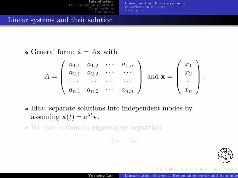
General form: x = Ax with
A =
a1,1 a1,2 · · · a1,n
a2,1 a2,2 · · · · · ·· · · · · · · · · · · ·an,1 an,2 · · · an,n
and x =
x1
x2
·xn
.
Idea: separate solutions into independent modes byassuming x(t) = eλtv.We then obtain an eigenvalue equation
Av = λv .
Yueheng Lan Linearization theorems, Koopman operator and its application
IntroductionThe Koopman operator
ApplicationsSummary
Linear and nonlinear dynamicslinearization in largeExamples
Linear systems and their solution
General form: x = Ax with
A =
a1,1 a1,2 · · · a1,n
a2,1 a2,2 · · · · · ·· · · · · · · · · · · ·an,1 an,2 · · · an,n
and x =
x1
x2
·xn
.
Idea: separate solutions into independent modes byassuming x(t) = eλtv.We then obtain an eigenvalue equation
Av = λv .
Yueheng Lan Linearization theorems, Koopman operator and its application

IntroductionThe Koopman operator
ApplicationsSummary
Linear and nonlinear dynamicslinearization in largeExamples
Linearization of nonlinear systems
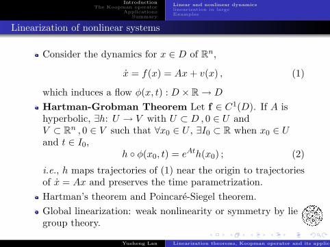
Consider the dynamics for x ∈ D of Rn,
x = f(x) = Ax + v(x) , (1)
which induces a flow φ(x, t) : D × R → D
Hartman-Grobman Theorem Let f ∈ C1(D). If A ishyperbolic, ∃h: U → V with U ⊂ D , 0 ∈ U andV ⊂ Rn , 0 ∈ V such that ∀x0 ∈ U , ∃I0 ⊂ R when x0 ∈ Uand t ∈ I0,
h φ(x0, t) = eAth(x0) ; (2)
i.e., h maps trajectories of (1) near the origin to trajectoriesof x = Ax and preserves the time parametrization.Hartman’s theorem and Poincare-Siegel theorem.Global linearization: weak nonlinearity or symmetry by liegroup theory.
Yueheng Lan Linearization theorems, Koopman operator and its application

IntroductionThe Koopman operator
ApplicationsSummary
Linear and nonlinear dynamicslinearization in largeExamples
Linearization of nonlinear systems
Consider the dynamics for x ∈ D of Rn,
x = f(x) = Ax + v(x) , (1)
which induces a flow φ(x, t) : D × R → D
Hartman-Grobman Theorem Let f ∈ C1(D). If A ishyperbolic, ∃h: U → V with U ⊂ D , 0 ∈ U andV ⊂ Rn , 0 ∈ V such that ∀x0 ∈ U , ∃I0 ⊂ R when x0 ∈ Uand t ∈ I0,
h φ(x0, t) = eAth(x0) ; (2)
i.e., h maps trajectories of (1) near the origin to trajectoriesof x = Ax and preserves the time parametrization.Hartman’s theorem and Poincare-Siegel theorem.Global linearization: weak nonlinearity or symmetry by liegroup theory.
Yueheng Lan Linearization theorems, Koopman operator and its application

IntroductionThe Koopman operator
ApplicationsSummary
Linear and nonlinear dynamicslinearization in largeExamples
Main contents
1 IntroductionLinear and nonlinear dynamicslinearization in largeExamples
2 The Koopman operatorIts introductionKoopman operator and partition of the phase space
3 ApplicationsThe standard mapApplication to fluid dynamics
4 Summary
Yueheng Lan Linearization theorems, Koopman operator and its application

IntroductionThe Koopman operator
ApplicationsSummary
Linear and nonlinear dynamicslinearization in largeExamples
Problems and general consideration
Problems in the current linearization scheme:Local theorems: too limited region of validity;Global theorems: linear terms dominate or a completesolution of the equation is required.
In essence, linearizability means a conjugacya nonlinear system ↔ a linear system
Thus(1) the linearizable region can contain only one equilibrium;(2) chaotic trajectories cannot be linearized;(3) At most one attractor or one repeller exists in theregion.
Yueheng Lan Linearization theorems, Koopman operator and its application
IntroductionThe Koopman operator
ApplicationsSummary
Linear and nonlinear dynamicslinearization in largeExamples
Autonomous flow linearization
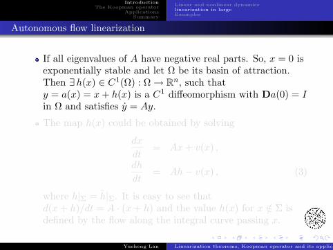
If all eigenvalues of A have negative real parts. So, x = 0 isexponentially stable and let Ω be its basin of attraction.Then ∃h(x) ∈ C1(Ω) : Ω → Rn, such thaty = a(x) = x + h(x) is a C1 diffeomorphism with Da(0) = Iin Ω and satisfies y = Ay.
The map h(x) could be obtained by solving
dx
dt= Ax + v(x) ,
dh
dt= Ah− v(x) , (3)
where h|Σ = h|Σ. It is easy to see thatd(x + h)/dt = A · (x + h) and the value h(x) for x /∈ Σ isdefined by the flow along the integral curve passing x.
Yueheng Lan Linearization theorems, Koopman operator and its application

IntroductionThe Koopman operator
ApplicationsSummary
Linear and nonlinear dynamicslinearization in largeExamples
Autonomous flow linearization
If all eigenvalues of A have negative real parts. So, x = 0 isexponentially stable and let Ω be its basin of attraction.Then ∃h(x) ∈ C1(Ω) : Ω → Rn, such thaty = a(x) = x + h(x) is a C1 diffeomorphism with Da(0) = Iin Ω and satisfies y = Ay.
The map h(x) could be obtained by solving
dx
dt= Ax + v(x) ,
dh
dt= Ah− v(x) , (3)
where h|Σ = h|Σ. It is easy to see thatd(x + h)/dt = A · (x + h) and the value h(x) for x /∈ Σ isdefined by the flow along the integral curve passing x.
Yueheng Lan Linearization theorems, Koopman operator and its application
IntroductionThe Koopman operator
ApplicationsSummary
Linear and nonlinear dynamicslinearization in largeExamples
The generalization
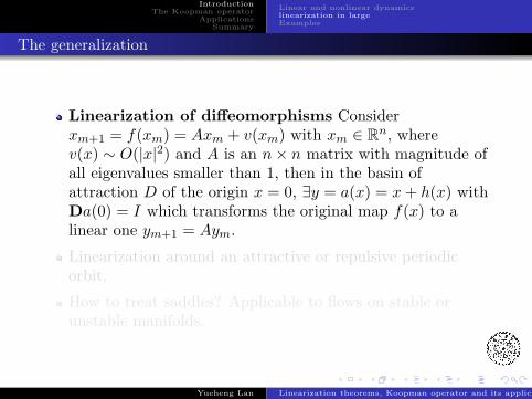
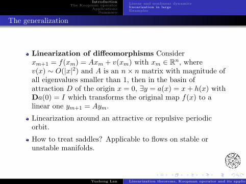
Linearization of diffeomorphisms Considerxm+1 = f(xm) = Axm + v(xm) with xm ∈ Rn, wherev(x) ∼ O(|x|2) and A is an n× n matrix with magnitude ofall eigenvalues smaller than 1, then in the basin ofattraction D of the origin x = 0, ∃y = a(x) = x + h(x) withDa(0) = I which transforms the original map f(x) to alinear one ym+1 = Aym.
Linearization around an attractive or repulsive periodicorbit.
How to treat saddles? Applicable to flows on stable orunstable manifolds.
Yueheng Lan Linearization theorems, Koopman operator and its application

IntroductionThe Koopman operator
ApplicationsSummary
Linear and nonlinear dynamicslinearization in largeExamples
The generalization
Linearization of diffeomorphisms Considerxm+1 = f(xm) = Axm + v(xm) with xm ∈ Rn, wherev(x) ∼ O(|x|2) and A is an n× n matrix with magnitude ofall eigenvalues smaller than 1, then in the basin ofattraction D of the origin x = 0, ∃y = a(x) = x + h(x) withDa(0) = I which transforms the original map f(x) to alinear one ym+1 = Aym.
Linearization around an attractive or repulsive periodicorbit.
How to treat saddles? Applicable to flows on stable orunstable manifolds.
Yueheng Lan Linearization theorems, Koopman operator and its application

IntroductionThe Koopman operator
ApplicationsSummary
Linear and nonlinear dynamicslinearization in largeExamples
Main contents
1 IntroductionLinear and nonlinear dynamicslinearization in largeExamples
2 The Koopman operatorIts introductionKoopman operator and partition of the phase space
3 ApplicationsThe standard mapApplication to fluid dynamics
4 Summary
Yueheng Lan Linearization theorems, Koopman operator and its application

IntroductionThe Koopman operator
ApplicationsSummary
Linear and nonlinear dynamicslinearization in largeExamples
Two examples
Consider the 1-d equation x = x− x3. The transformation
x = b(y) =y√
1 + y2
results in y = y, valid for x ∈ [−1, 1].
Consider the 2-d system z1 = 2z1 , z2 = 4z2 + z21 . The
transformation
z1 = y1 , z2 = y2 + t(y1, y2)y21
where t(y1, y2) = 14 ln y2
1 results in
y1 = 2y1 , y2 = 4y2 .
[Y. Lan and I. Mezic, Physica D. 242, 42(2013)]
Yueheng Lan Linearization theorems, Koopman operator and its application

IntroductionThe Koopman operator
ApplicationsSummary
Its introductionKoopman operator and partition of the phase space
Main contents
1 IntroductionLinear and nonlinear dynamicslinearization in largeExamples
2 The Koopman operatorIts introductionKoopman operator and partition of the phase space
3 ApplicationsThe standard mapApplication to fluid dynamics
4 Summary
Yueheng Lan Linearization theorems, Koopman operator and its application

IntroductionThe Koopman operator
ApplicationsSummary
Its introductionKoopman operator and partition of the phase space
Remarks on the linearization theorem
A nonlinear system can be linearized in the whole basin ofattraction of an equilibrium or a periodic orbit. Accordingto the Morse theory, the whole phase space can be viewedas a gradient system quotient the minimal transitiveinvariant sets. The phase space is a juxtaposition oflinearizable patches.The theorems are existence ones and it is hard to identifyexactly the linearization transformation.At present, theorems are only proved for equilibria andperiodic orbits.Without explicit analytic expression, it is hard to deducethe linearization from experimental observation.
Yueheng Lan Linearization theorems, Koopman operator and its application

IntroductionThe Koopman operator
ApplicationsSummary
Its introductionKoopman operator and partition of the phase space
Koopman operator, a way out?
A statistical point of view:Evolution of densities: the Perron-Frobinius Operator inanalogy with the Schrodinger picture;Evolution of observables: the Koopman operator in analogywith the Heisenberg picture.Definition: for a map xn+1 = f(xn) and a function g(x), theKoopman operator U g(x) = g(f(x))For a flow φ(x, t) and a function g(x), a semigroup ofKoopman operators could be defined asUt g(x) = g(φ(x, t)).
Yueheng Lan Linearization theorems, Koopman operator and its application

IntroductionThe Koopman operator
ApplicationsSummary
Its introductionKoopman operator and partition of the phase space
Eigenvalues and eigenmodes
It is a linear operator, which is unitary on a transitiveinvariant set.The eigenvalues and eigenmodes are interesting objects.For a 1-d linear map xn+1 = λxn and observable g(x) = xn,
U g(x) = (λx)n = λnxn .
For a 1-d equation x = λx and observable g(x) = xn
Ut g(x) = (xeλt)n = enλtxn .
Yueheng Lan Linearization theorems, Koopman operator and its application

IntroductionThe Koopman operator
ApplicationsSummary
Its introductionKoopman operator and partition of the phase space
Nontrivial examples
Note that h(x) in the Hartman-Grobman’s theorem satisfies
Uth(x) = h φ(x, t) = eAth(x)
SupposeV −1AV = Λ ,
then we get
V −1h φ(x, t) = V −1eAth(x),
and so k = V −1h satisfies
k φ(x0, t) = eΛtk(x0)
i.e. each component function of k is an eigenfunction of Ut.
Yueheng Lan Linearization theorems, Koopman operator and its application

IntroductionThe Koopman operator
ApplicationsSummary
Its introductionKoopman operator and partition of the phase space
Main contents
1 IntroductionLinear and nonlinear dynamicslinearization in largeExamples
2 The Koopman operatorIts introductionKoopman operator and partition of the phase space
3 ApplicationsThe standard mapApplication to fluid dynamics
4 Summary
Yueheng Lan Linearization theorems, Koopman operator and its application

IntroductionThe Koopman operator
ApplicationsSummary
Its introductionKoopman operator and partition of the phase space
Construction of eigenmodes along trajectories
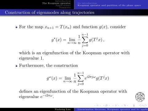
For the map xn+1 = T (xn) and function g(x), consider
g∗(x) = limn→∞
1n
n−1∑j=0
g(T jx) ,
which is an eigenfunction of the Koopman operator witheigenvalue 1.
Furthermore, the construction
gω(x) = limn→∞
1n
n−1∑j=0
ei2πjωg(T jx)
defines an eigenfunction of the Koopman operator witheigenvalue e−i2πω.
Yueheng Lan Linearization theorems, Koopman operator and its application
IntroductionThe Koopman operator
ApplicationsSummary
Its introductionKoopman operator and partition of the phase space
Construction of eigenmodes along trajectories
For the map xn+1 = T (xn) and function g(x), consider
g∗(x) = limn→∞
1n
n−1∑j=0
g(T jx) ,
which is an eigenfunction of the Koopman operator witheigenvalue 1.
Furthermore, the construction
gω(x) = limn→∞
1n
n−1∑j=0
ei2πjωg(T jx)
defines an eigenfunction of the Koopman operator witheigenvalue e−i2πω.
Yueheng Lan Linearization theorems, Koopman operator and its application

IntroductionThe Koopman operator
ApplicationsSummary
Its introductionKoopman operator and partition of the phase space
Spectral decomposition of evolution equations
For an evolution equation in an infinite-dimensional Hilbertspace v(x)n+1 = N(v(x)n, p) and if the attractor M is offinite dimension with the evolution mn+1 = T (mn).For an observable g(x,m), we have
Ug(x,m) = Usg(x,m) + Urg(x,m)
= g∗(x) +k∑
j=1
λjfj(m)gj(x) +∫ 1
0ei2παdE(α)g(x,m) .
Us: the singular part of the operator corresponding to thediscrete part of the spectrum, viewed as a deterministicpart.Ur: the regular part of the operator corresponding to thecontinuous part of the spectrum, viewed as a stochasticpart.
[I. Mezic, Nonlinear Dynamics 41, 309(2005)]Yueheng Lan Linearization theorems, Koopman operator and its application

IntroductionThe Koopman operator
ApplicationsSummary
The standard mapApplication to fluid dynamics
Main contents
1 IntroductionLinear and nonlinear dynamicslinearization in largeExamples
2 The Koopman operatorIts introductionKoopman operator and partition of the phase space
3 ApplicationsThe standard mapApplication to fluid dynamics
4 Summary
Yueheng Lan Linearization theorems, Koopman operator and its application

IntroductionThe Koopman operator
ApplicationsSummary
The standard mapApplication to fluid dynamics
The standard map
The Chirikov standardmap is
x∗1 = x1+2πε sin(x2)(mod2π)
x∗2 = x∗1 + x2(mod2π)
The embedding ofdynamics into space ofthree observables.[M. Budisic and I. Mezic,48th IEEE Conferenceon Decision and Control]
Yueheng Lan Linearization theorems, Koopman operator and its application

IntroductionThe Koopman operator
ApplicationsSummary
The standard mapApplication to fluid dynamics
Several eigenmodes of the Koopman operator
Eigenvectors for λ1 , λ2 , λ7 , λ17 at ε = 0.133.
Yueheng Lan Linearization theorems, Koopman operator and its application

IntroductionThe Koopman operator
ApplicationsSummary
The standard mapApplication to fluid dynamics
Main contents
1 IntroductionLinear and nonlinear dynamicslinearization in largeExamples
2 The Koopman operatorIts introductionKoopman operator and partition of the phase space
3 ApplicationsThe standard mapApplication to fluid dynamics
4 Summary
Yueheng Lan Linearization theorems, Koopman operator and its application

IntroductionThe Koopman operator
ApplicationsSummary
The standard mapApplication to fluid dynamics
Fluid dynamics
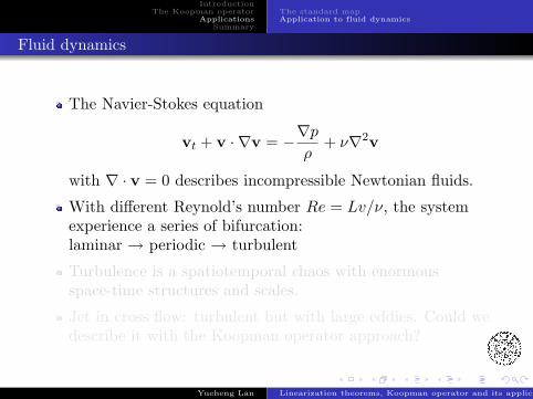
The Navier-Stokes equation
vt + v · ∇v = −∇p
ρ+ ν∇2v
with ∇ · v = 0 describes incompressible Newtonian fluids.
With different Reynold’s number Re = Lv/ν, the systemexperience a series of bifurcation:laminar → periodic → turbulent
Turbulence is a spatiotemporal chaos with enormousspace-time structures and scales.
Jet in cross flow: turbulent but with large eddies. Could wedescribe it with the Koopman operator approach?
Yueheng Lan Linearization theorems, Koopman operator and its application
IntroductionThe Koopman operator
ApplicationsSummary
The standard mapApplication to fluid dynamics
Fluid dynamics
The Navier-Stokes equation
vt + v · ∇v = −∇p
ρ+ ν∇2v
with ∇ · v = 0 describes incompressible Newtonian fluids.
With different Reynold’s number Re = Lv/ν, the systemexperience a series of bifurcation:laminar → periodic → turbulent
Turbulence is a spatiotemporal chaos with enormousspace-time structures and scales.
Jet in cross flow: turbulent but with large eddies. Could wedescribe it with the Koopman operator approach?
Yueheng Lan Linearization theorems, Koopman operator and its application

IntroductionThe Koopman operator
ApplicationsSummary
The standard mapApplication to fluid dynamics
Jet in cross flow
[C. W. Rowley et al, J. Fluid Mech. 641, 115(2009)]
Yueheng Lan Linearization theorems, Koopman operator and its application

IntroductionThe Koopman operator
ApplicationsSummary
The standard mapApplication to fluid dynamics
The Arnoldi algorithm
Consider a linear dynamical system xk+1 = Axk andconstruct the matrix
K = [x0 , x1 , · · · , xm−1] = [x0 , Ax0 , · · · , Am−1x0] .
If the mth iterate xm = Axm−1 =∑m−1
k=0 ckxk + r, the wecan write AK ≈ KC, where
C =
0 0 0 · · · c0
1 0 0 · · · c1
0 1 0 · · · c2
· · · · · ·0 · · · 0 1 c0
.
If Ca = λa, then the value λ and the vector v = Ka areapproximate eigenvalue and eigenvector of the originalmatrix A.
Yueheng Lan Linearization theorems, Koopman operator and its application

IntroductionThe Koopman operator
ApplicationsSummary
The standard mapApplication to fluid dynamics
Two structure functions
The two eigenmodes
Yueheng Lan Linearization theorems, Koopman operator and its application

IntroductionThe Koopman operator
ApplicationsSummary
Summary
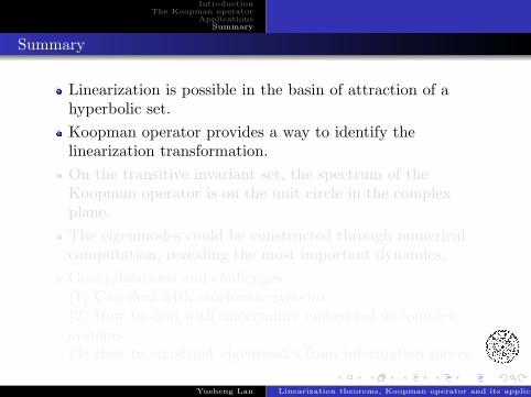
Linearization is possible in the basin of attraction of ahyperbolic set.Koopman operator provides a way to identify thelinearization transformation.On the transitive invariant set, the spectrum of theKoopman operator is on the unit circle in the complexplane.The eigenmodes could be constructed through numericalcomputation, revealing the most important dynamics.Generalizations and challenges:(1) Can deal with stochastic systems.(2) How to deal with uncertainty embedded in complexsystems.(3) How to construct eigenmodes from information pieces.
Yueheng Lan Linearization theorems, Koopman operator and its application
IntroductionThe Koopman operator
ApplicationsSummary
Summary
Linearization is possible in the basin of attraction of ahyperbolic set.Koopman operator provides a way to identify thelinearization transformation.On the transitive invariant set, the spectrum of theKoopman operator is on the unit circle in the complexplane.The eigenmodes could be constructed through numericalcomputation, revealing the most important dynamics.Generalizations and challenges:(1) Can deal with stochastic systems.(2) How to deal with uncertainty embedded in complexsystems.(3) How to construct eigenmodes from information pieces.
Yueheng Lan Linearization theorems, Koopman operator and its application