Linear VS Nonlinear buckling

piotr.stepien@midasit.com

Piotr Stepien,

CAE Engineer

NFX International Support

Structural stability and Buckling

Phenomenon

Buckling Phenomenon

Buckling is an instability of equilibrium in structures that occurs from compressive loads or

stresses. A structure or its components may fail due to buckling at loads that are far smaller

than those that produce material strength failure.

Buckling is a catastrophic failure.

As strange as it may sound, thecolumn behind a steering wheel isdesigned to fail and buckle during acar crash to prevent impaling thedriver.

Structural stability and Buckling

Phenomenon

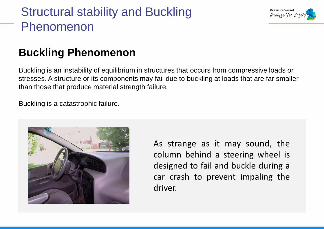
In contrast, the columns of abuilding are designed so they do notbuckle under the weight of thebuilding. Buckling in this caserepresents the instability of thecolumns under compression.

If a compressive axial force isapplied to a long, thin wooden strip,then it will bend significantly.

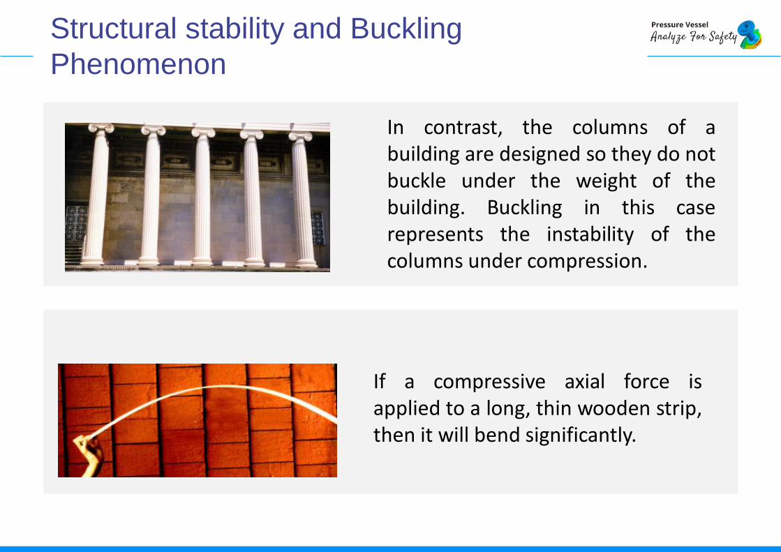
Any structure can be easily weakened bybuckling and experience sudden andcatastrophic collapse.

Under which conditions will a compressiveaxial force produce only axial contractionand when does it produce bending?

When is the bending caused by axial loadscatastrophic? How can you design toprevent catastrophic failure from axialloads?

Structural stability and Buckling

Phenomenon

Euler buckling

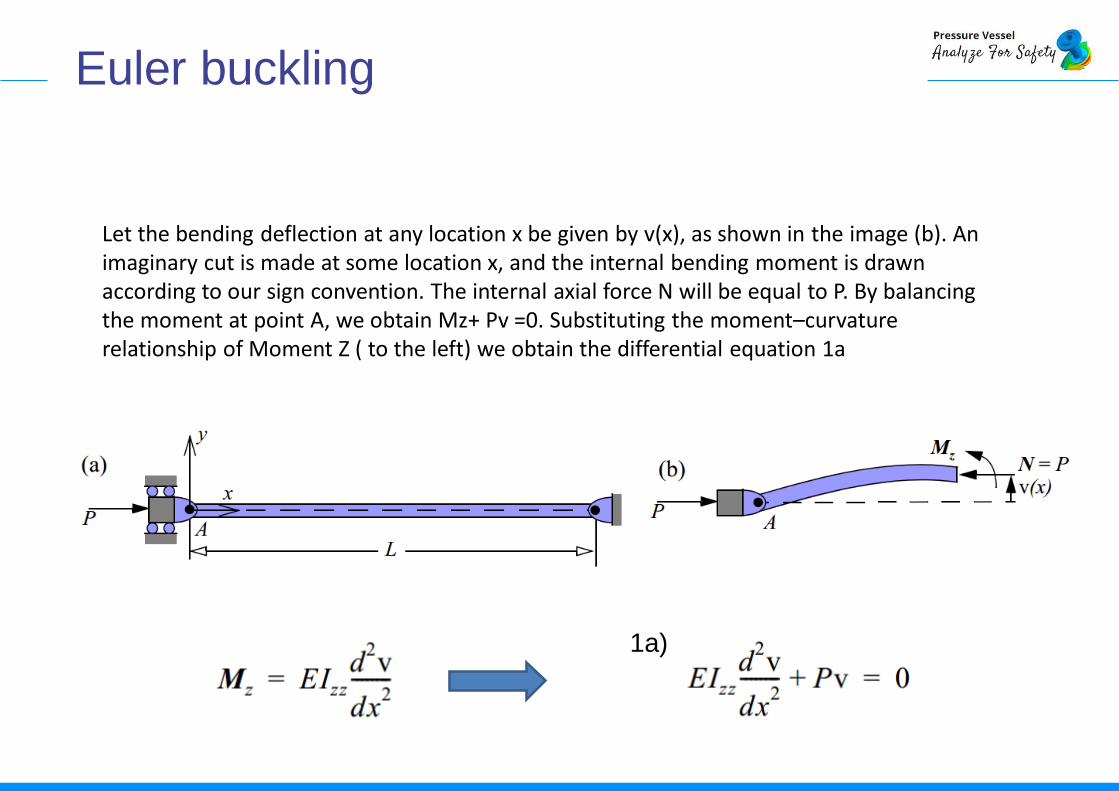
Let the bending deflection at any location x be given by v(x), as shown in the image (b). An imaginary cut is made at some location x, and the internal bending moment is drawn according to our sign convention. The internal axial force N will be equal to P. By balancing the moment at point A, we obtain Mz+ Pv =0. Substituting the moment–curvature relationship of Moment Z ( to the left) we obtain the differential equation 1a

1a)

Differential Equation Boundary Conditions

where

1a)

1b) 1c)2a)

2b)

Euler buckling

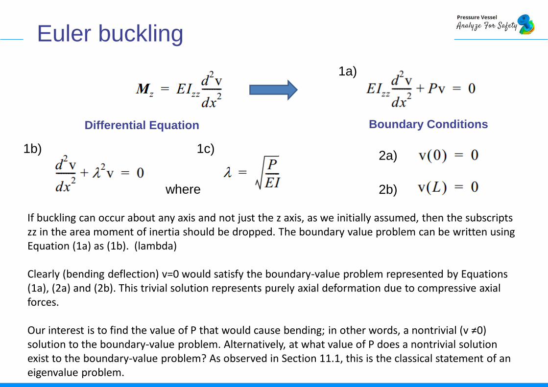
If buckling can occur about any axis and not just the z axis, as we initially assumed, then the subscripts zz in the area moment of inertia should be dropped. The boundary value problem can be written using Equation (1a) as (1b). (lambda)

Clearly (bending deflection) v=0 would satisfy the boundary-value problem represented by Equations (1a), (2a) and (2b). This trivial solution represents purely axial deformation due to compressive axial forces.

Our interest is to find the value of P that would cause bending; in other words, a nontrivial (v ≠0) solution to the boundary-value problem. Alternatively, at what value of P does a nontrivial solution exist to the boundary-value problem? As observed in Section 11.1, this is the classical statement of an eigenvalue problem.

Differential Equation

Characteristic equation or the buckling equation

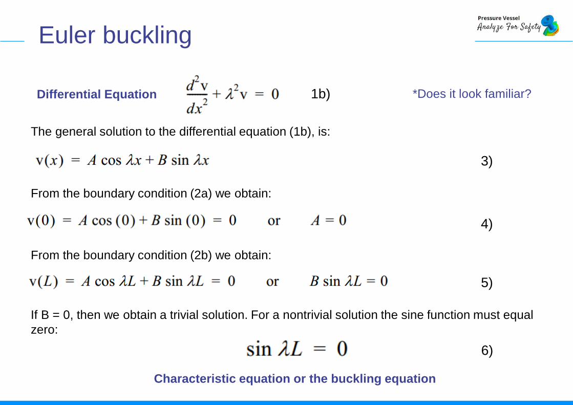
The general solution to the differential equation (1b), is:

*Does it look familiar?

From the boundary condition (2a) we obtain:

From the boundary condition (2b) we obtain:

If B = 0, then we obtain a trivial solution. For a nontrivial solution the sine function must equal

zero:

3)

4)

5)

1b)

6)

Euler buckling

Euler buckling

Characteristic Equation 6)

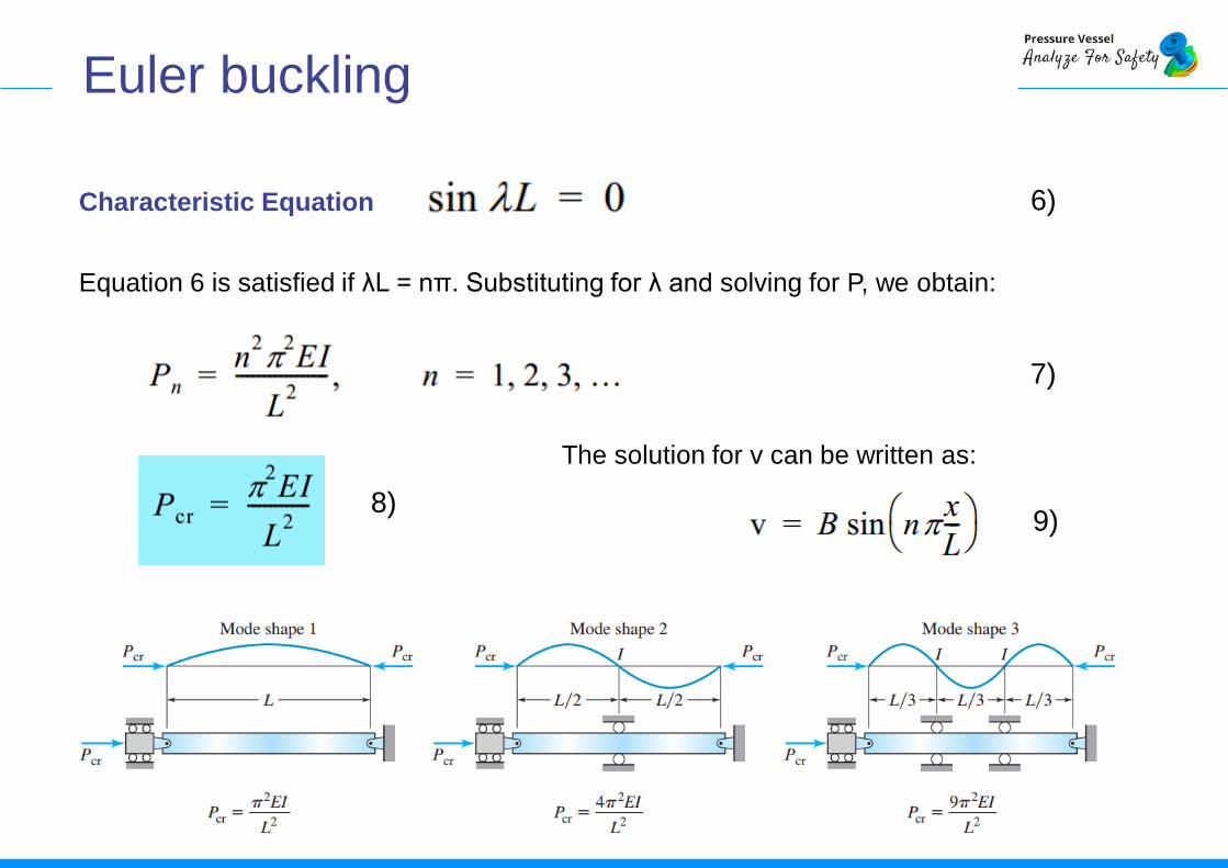
Equation 6 is satisfied if λL = nπ. Substituting for λ and solving for P, we obtain:

7)

8)9)

The solution for v can be written as:

Euler buckling

Equation (8) represents the values of load P(the eigenvalues) at which buckling would occur. What is the lowest value of P at which buckling will occur? Clearly, for the lowest value of P, n should equal 1 in Equation (7). Furthermore minimum value of I (cross sectional moment of Inertia) should be used. The critical buckling load is like on equation 8.

Pcr, the critical buckling load, is also called Euler load. Buckling will occur about the axis that has minimum area moment of inertia.

Equation (9) represents the buckled mode(eigenvectors). Notice that the constant B in Equation 9 is undetermined. This is typical in eigenvalue problems. The importance of each buckled mode shape can be appreciated by examining Figure below. If buckled mode 1 is prevented from occurring by installing a restraint (or support), then the column would buckle at the next higher mode at critical load values that are higher than those for the lower modes. Point I on the deflection curves describing the mode shapes has two attributes: it is an inflection point and the magnitude of deflection at this point is zero.

Recall that the curvature d2v/dx2 (second derivative for deflection) at an inflection point is zero. Hence the internal moment Mz at this point is zero. If roller supports are put at any other points than the inflection points I, as predicted by Equation (9), then the boundary-value problem will have different eigenvalues (critical loads) and eigenvectors (mode shapes).

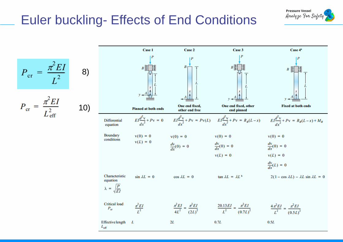
Euler buckling- Effects of End Conditions

10)

8)

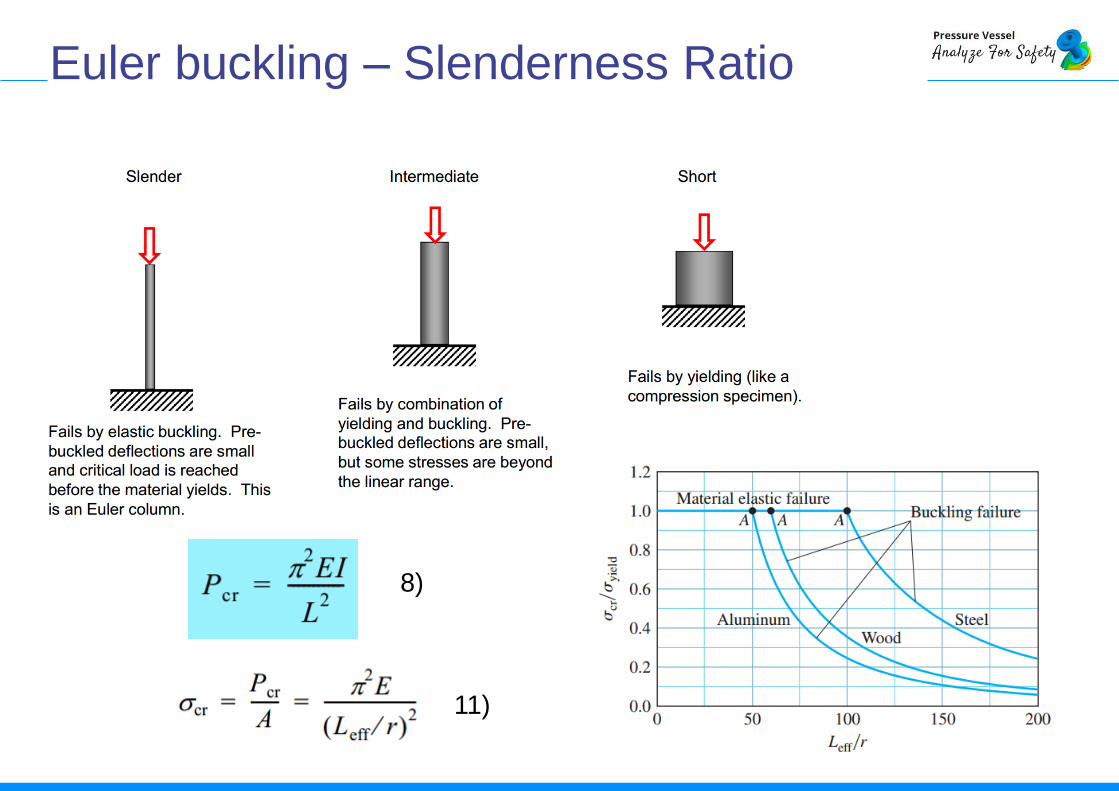
Euler buckling – Slenderness Ratio

11)

8)

Euler buckling – Slenderness RatioIn Equation (9), I (moment of inertia) can be replaced by Ar2 ,where A is the cross-sectional area and r is the minimum radius of gyration.We obtain (12) where Leff /r is the slenderness ratio and σcr is the compressive axial stress just before the column would buckle. Equation (12) is valid only in the elastic region—that is, if σcr < σyield . If σcr > σyield , then elastic failure will be due to stress exceeding the material strength. Thus σcr=σyielddefines the failure envelope for a column. Figure shows the failure envelopes for steel, aluminum, and wood. As nondimensional variables are used in the plots in Figure 10, these plots can also be used for metric units. Note that the slenderness ratio is defined using effective lengths; hence these plots are applicable to columns with different supports.

The failure envelopes in Figure 10 show that as the slenderness ratio increases, the failure due to buckling will occur at stress values significantly lower than the yield stress. This underscores the importance of buckling in the design of members under compression.

The failure envelopes, as shown in Figure 10, depend only on the material property and are applicable to columns of different lengths, shapes, and types of support. These failure envelopes are used for classifying columns as short or long.

Short column design is based on using yield stress as the failure stress. Long column design is based on using critical buckling stress as the failure stress. The slenderness ratio at point A for each material is used for separating short columns from long columns for that material. Point A is the intersection point of the straight line representing elastic material failure and the hyperbola curve representing buckling failure.

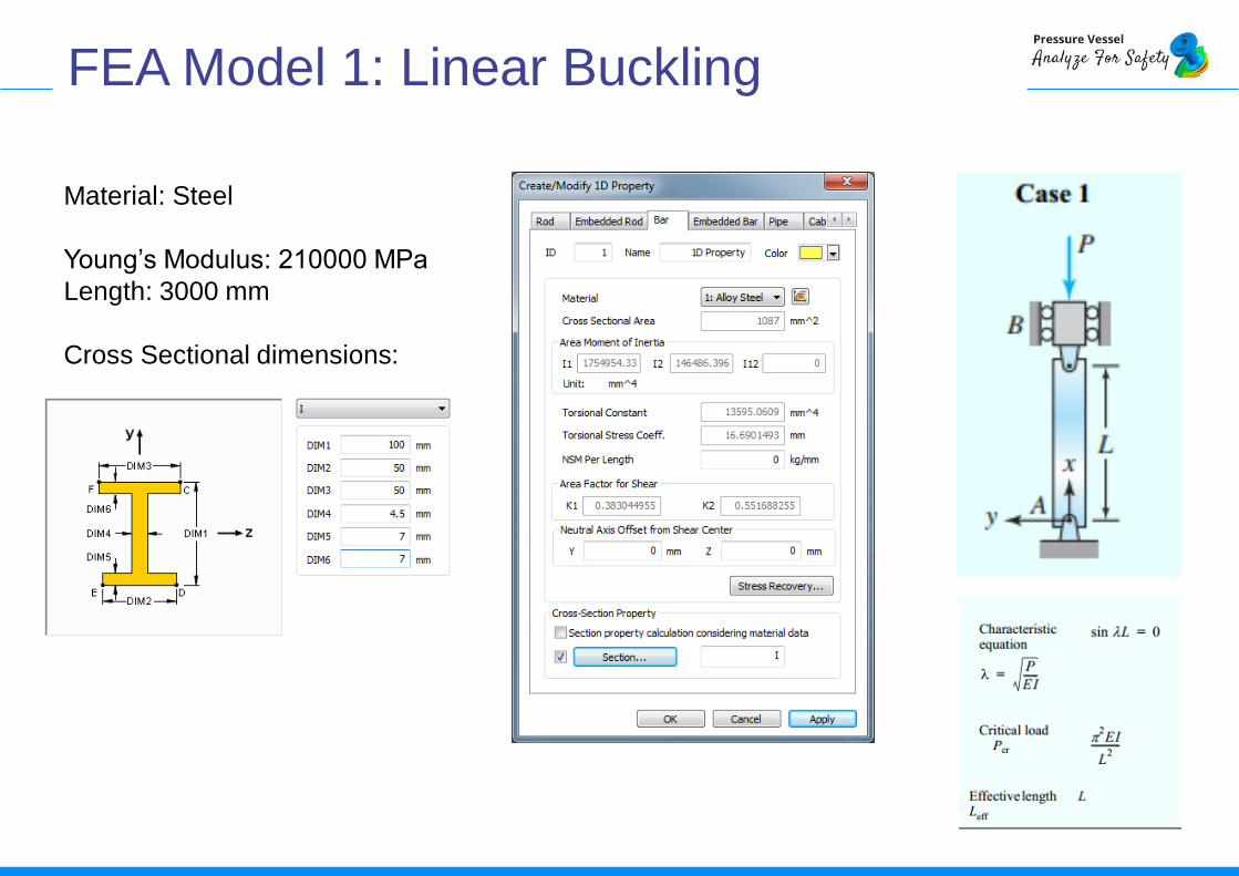
FEA Model 1: Linear Buckling

Material: Steel

Young’s Modulus: 210000 MPa

Length: 3000 mm

Cross Sectional dimensions:

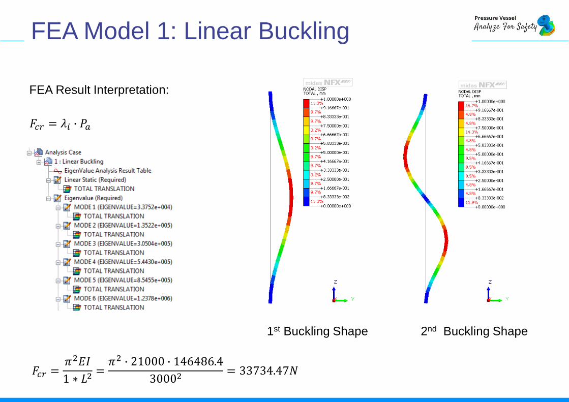
FEA Result Interpretation:

1st Buckling Shape 2nd Buckling Shape

𝐹𝑐𝑟 =𝜋2𝐸𝐼

1 ∗ 𝐿2=𝜋2 ∙ 21000 ∙ 146486.4

30002= 33734.47𝑁

𝐹𝑐𝑟 = 𝜆𝑖 ∙ 𝑃𝑎

FEA Model 1: Linear Buckling

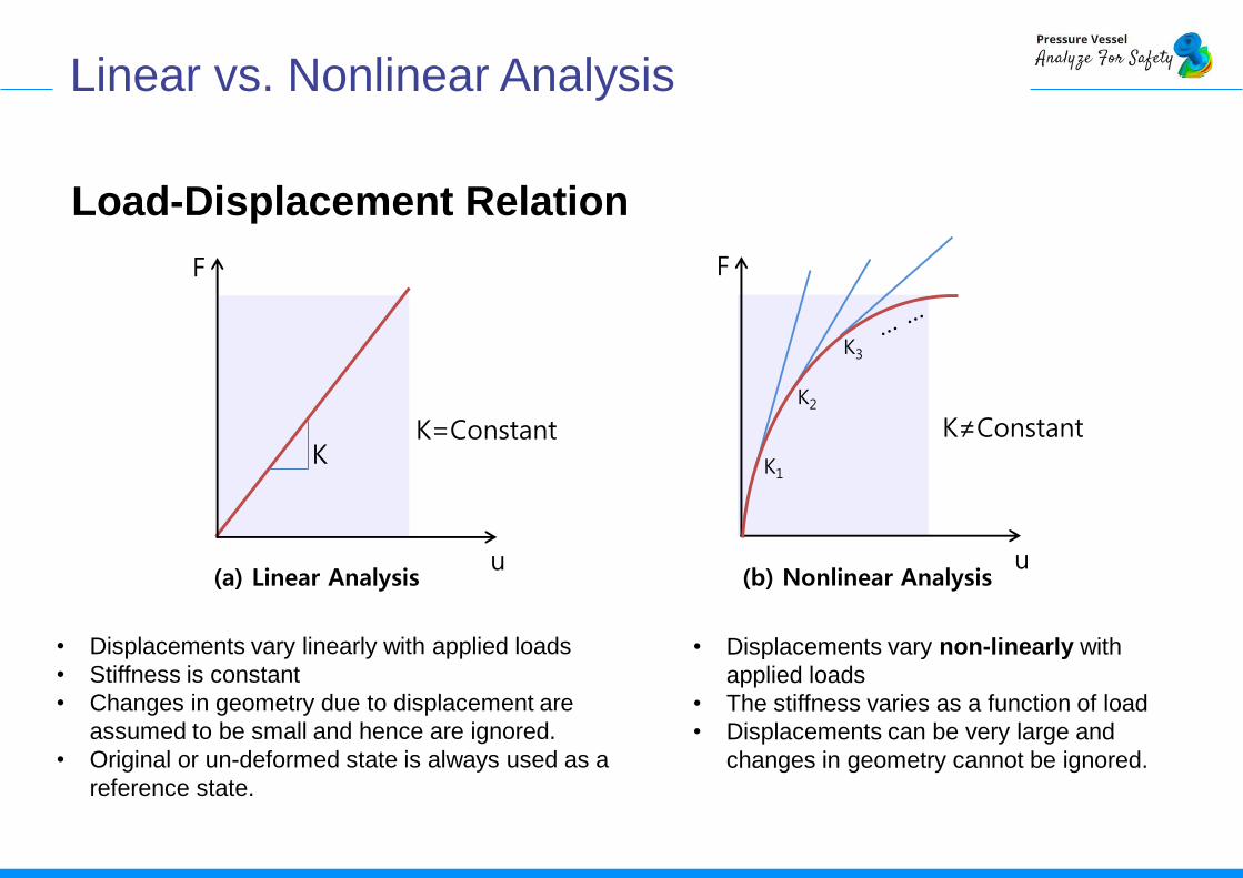
Linear vs. Nonlinear Analysis

Load-Displacement Relation

F

u

K

F

u

K=Constant K≠Constant

(a) Linear Analysis (b) Nonlinear Analysis

K1

K2

K3

• Displacements vary linearly with applied loads

• Stiffness is constant

• Changes in geometry due to displacement are

assumed to be small and hence are ignored.

• Original or un-deformed state is always used as a

reference state.

• Displacements vary non-linearly with

applied loads

• The stiffness varies as a function of load

• Displacements can be very large and

changes in geometry cannot be ignored.

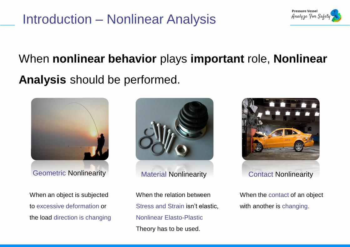
Geometric Nonlinearity Material Nonlinearity Contact Nonlinearity

When the contact of an object

with another is changing.

When an object is subjected

to excessive deformation or

the load direction is changing

When the relation between

Stress and Strain isn’t elastic,

Nonlinear Elasto-Plastic

Theory has to be used.

Introduction – Nonlinear Analysis

When nonlinear behavior plays important role, Nonlinear

Analysis should be performed.

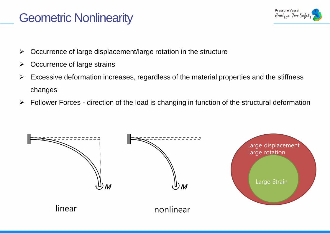
Occurrence of large displacement/large rotation in the structure

Occurrence of large strains

Excessive deformation increases, regardless of the material properties and the stiffness

changes

Follower Forces - direction of the load is changing in function of the structural deformation

MM

linear nonlinear

Geometric Nonlinearity

Large displacementLarge rotation

Large Strain

Geometric Nonlinearity

u

F

u

F

Limit point

u

F

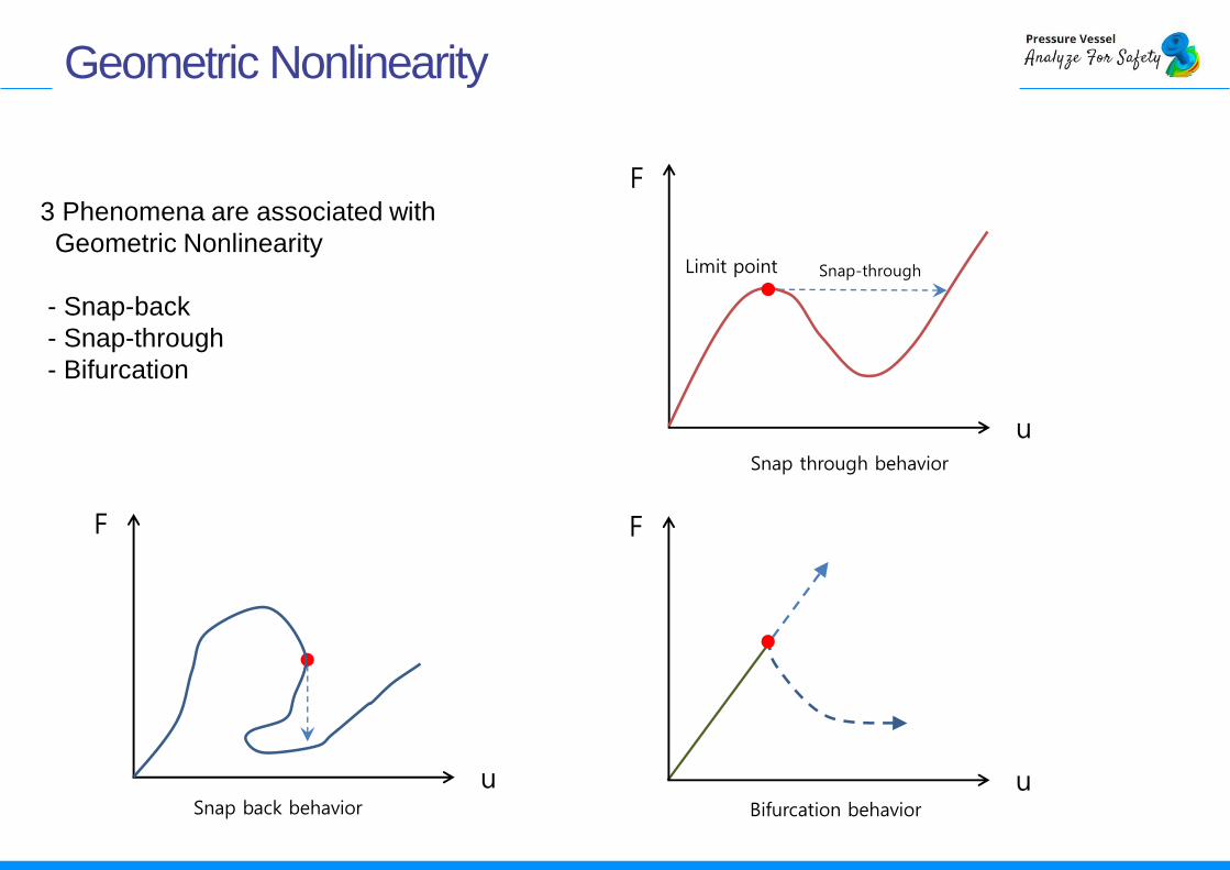
3 Phenomena are associated with

Geometric Nonlinearity

- Snap-back

- Snap-through

- Bifurcation

Snap through behavior

Bifurcation behaviorSnap back behavior

Snap-through

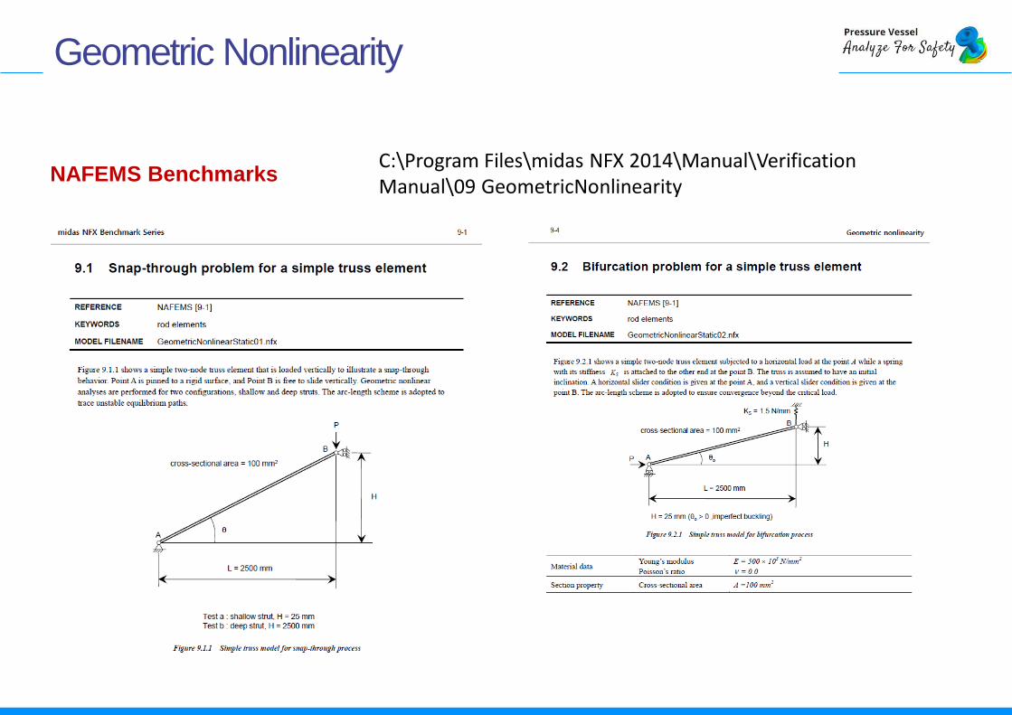
Geometric Nonlinearity

NAFEMS BenchmarksC:\Program Files\midas NFX 2014\Manual\Verification Manual\09 GeometricNonlinearity

F

u

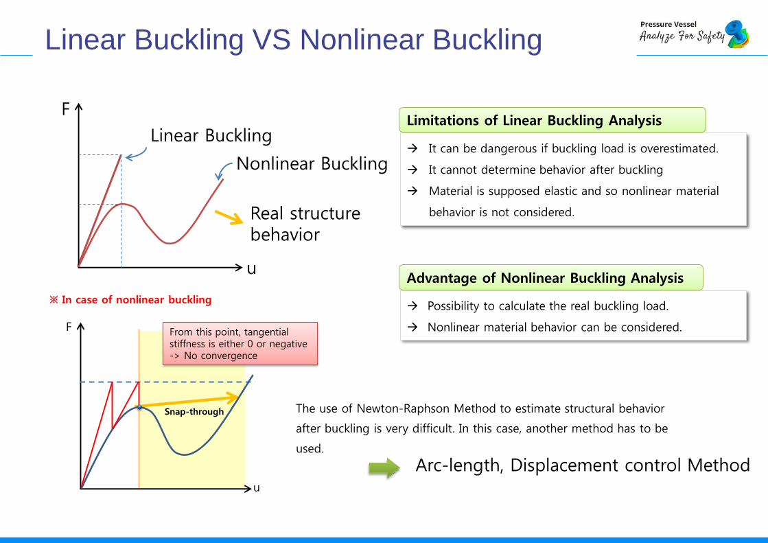
Nonlinear Buckling

Linear Buckling

Real structure behavior

It can be dangerous if buckling load is overestimated.

It cannot determine behavior after buckling

Material is supposed elastic and so nonlinear material

behavior is not considered.

Possibility to calculate the real buckling load.

Nonlinear material behavior can be considered.F

u

From this point, tangential stiffness is either 0 or negative -> No convergence

Snap-through

Limitations of Linear Buckling Analysis

Advantage of Nonlinear Buckling Analysis

Arc-length, Displacement control Method

The use of Newton-Raphson Method to estimate structural behavior

after buckling is very difficult. In this case, another method has to be

used.

※ In case of nonlinear buckling

Linear Buckling VS Nonlinear Buckling

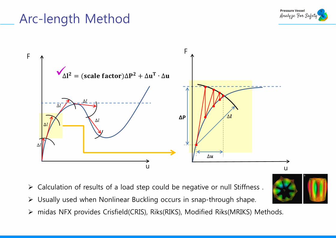
ΔP

F

u

Calculation of results of a load step could be negative or null Stiffness .

Usually used when Nonlinear Buckling occurs in snap-through shape.

midas NFX provides Crisfield(CRIS), Riks(RIKS), Modified Riks(MRIKS) Methods.

F

u

Arc-length Method

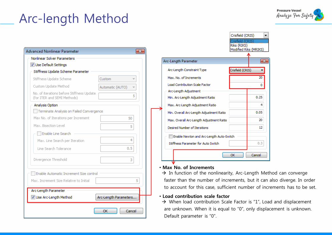
• Max No. of Increments In function of the nonlinearity, Arc-Length Method can converge

faster than the number of increments, but it can also diverge. In order

to account for this case, sufficient number of increments has to be set.

• Load contribution scale factor When load contribution Scale Factor is “1”, Load and displacement

are unknown. When it is equal to “0”, only displacement is unknown.

Default parameter is “0”.

Arc-length Method

Nonlinear Buckling Examples

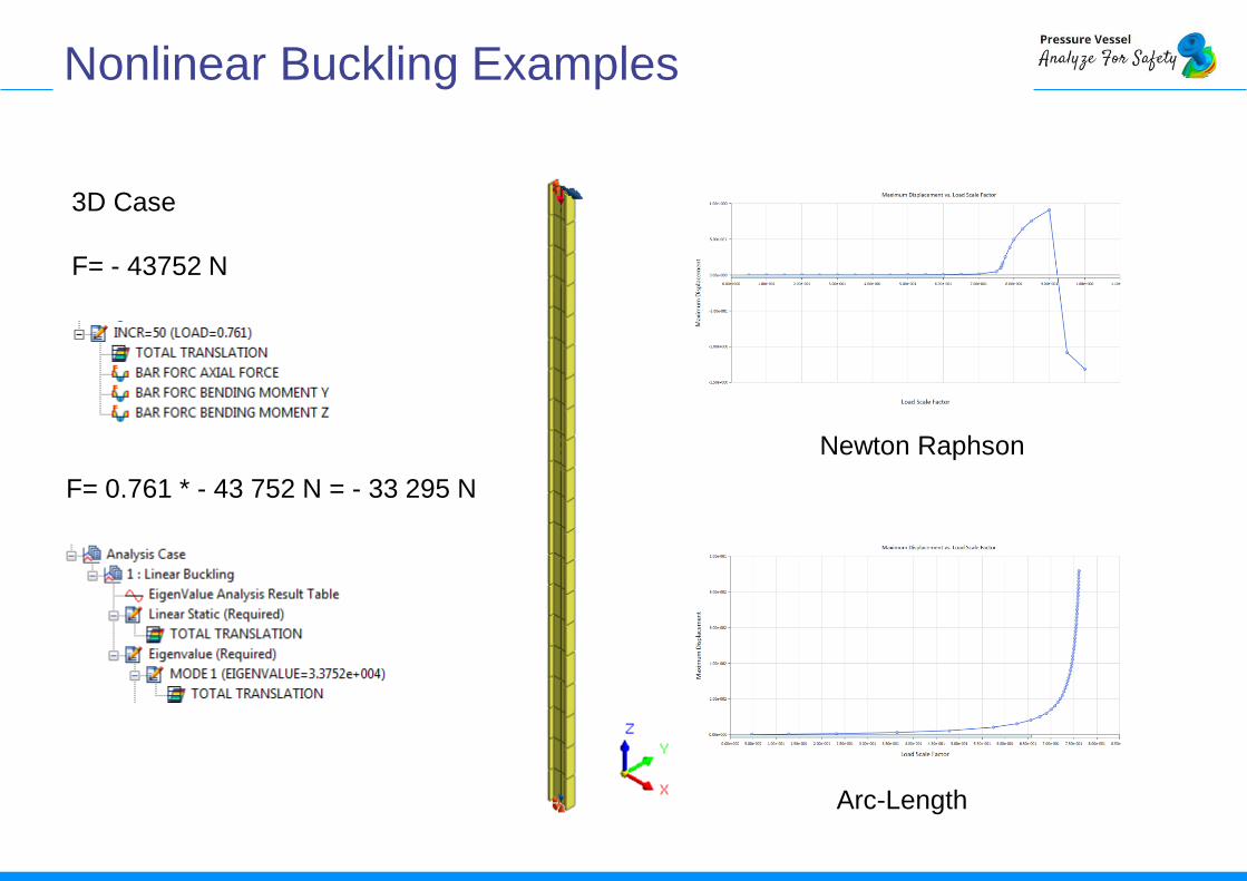
Newton Raphson

Arc-Length

3D Case

F= - 43752 N

F= 0.761 * - 43 752 N = - 33 295 N

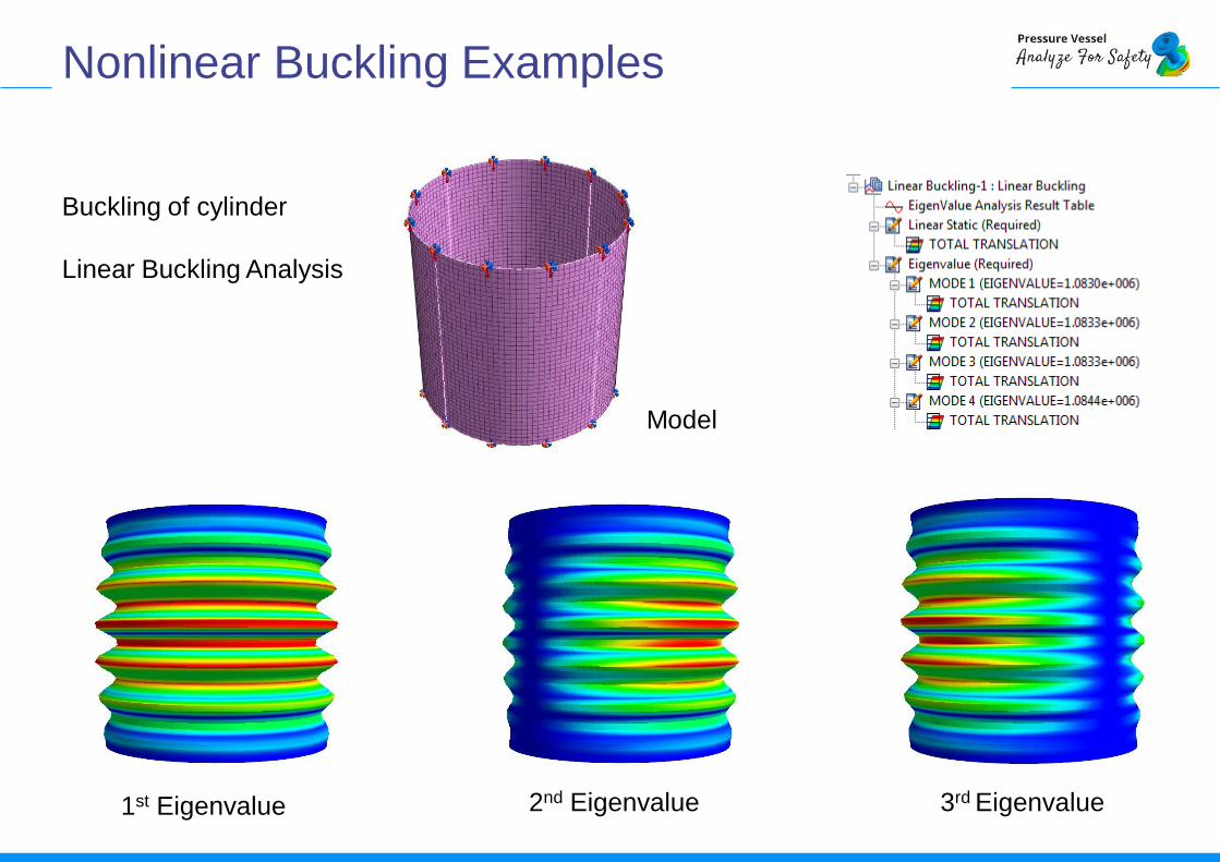
Buckling of cylinder

Linear Buckling Analysis

1st Eigenvalue 2nd Eigenvalue 3rd Eigenvalue

Model

Nonlinear Buckling Examples

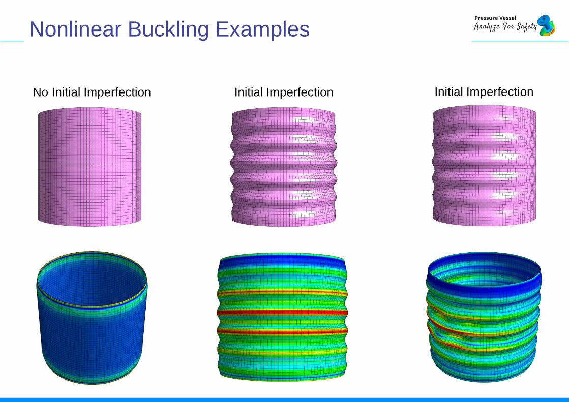
No Initial Imperfection Initial Imperfection Initial Imperfection

Nonlinear Buckling Examples

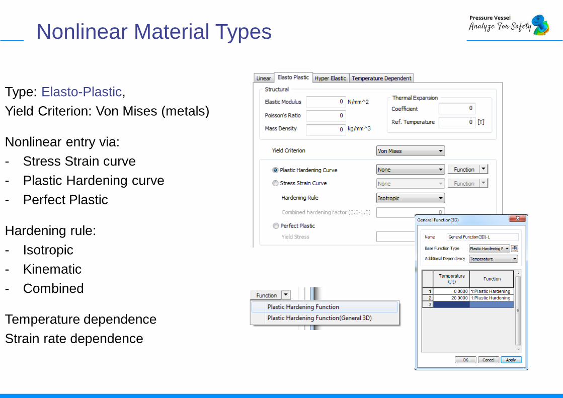
Type: Elasto-Plastic,

Yield Criterion: Von Mises (metals)

Nonlinear entry via:

- Stress Strain curve

- Plastic Hardening curve

- Perfect Plastic

Hardening rule:

- Isotropic

- Kinematic

- Combined

Temperature dependence

Strain rate dependence

Nonlinear Material Types

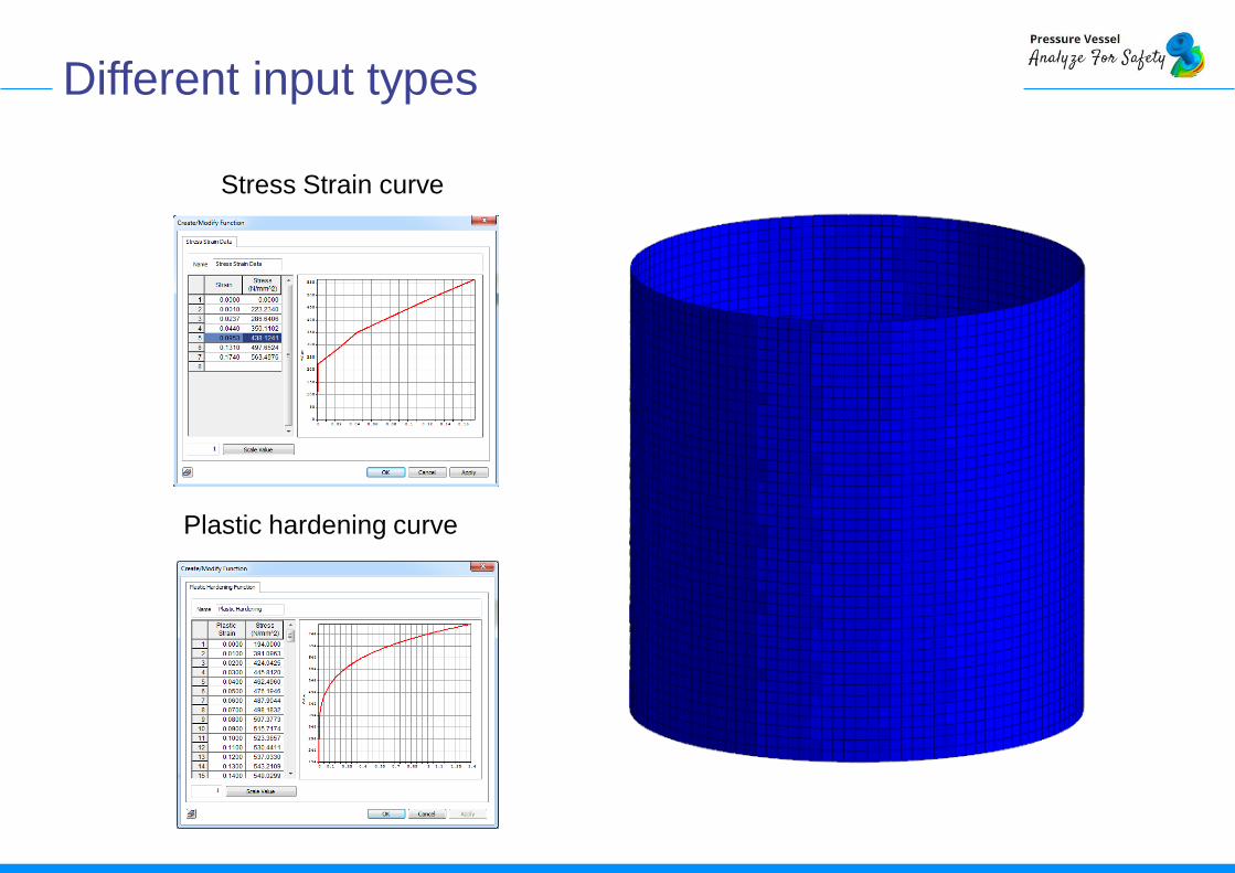
Stress Strain curve

Plastic hardening curve

Different input types

1. Know your goal and analysis purpose. Prepare a list of questions you think your analysis should be able to answer. Design the analysis, including the model, material model, and boundary conditions, in order to answer the questions you have in mind.

2. Try to understand the software’s supporting documentation, especially its output and warnings to be independent in case of solving potential problems. For example many users are not applying Boundary Conditions correctly, so it good to know how the software returns this information.

3. Learn first how the software works. You can prepare a simple model before you use a nonlinear feature which you haven’t used . Also guess how your structural component will behave, i.e. check for available studies, reports and benchmarks .

Essentials Steps in Nonlinear FEA

4. Keep the final model as simple as possible. A simple linear analysis done first can provide a lot of information such as where are the high stresses in the model, where the initial contact may occur, and what level of load will introduce plasticity in the model. The results of the linear analysis may even point out that there is no need for a nonlinear analysis. Examples of such a situation include the yield limit not being reached, there is no contact, and the displacements are small.

5. Try to look into the assumptions made with respect to the structural component, its geometry behavior with respect to large strain (if it is On or Off), look into different material models if the earlier model is unable to give you a result you expect (sometimes software only make some models compatible with commonly used elements and in this case you might look into a possibility of changing the element formulation).

6. Verify and validate the results of the nonlinear FEA solution. Verification means that “the model is computed correctly” from the numerical point of view. Wrong discretization with respect to the mesh size and time stepping are common errors. Validation asks the questions if “the correct model” is computed e.g. the geometry, material, boundary conditions, interactions etc. coincide with the one acting in reality.

Essentials Steps in Nonlinear FEA

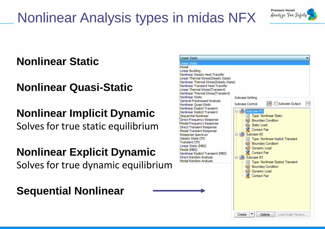
Nonlinear Static

Nonlinear Quasi-Static

Nonlinear Implicit DynamicSolves for true static equilibrium

Nonlinear Explicit DynamicSolves for true dynamic equilibrium

Sequential Nonlinear

Nonlinear Analysis types in midas NFX

A static analysis, like a stress analysis in FEA, is done using the simple linear equation [A]{x}={B}. In such analysis time does not play any role. On the other hand a dynamic analysis (or transient or modal analysis also) follows a more complex governing equation which is like: [M]{x''}+[C]{x'}+[K]{x}={F}

Implicit solution is one in which the calculation of current quantities in one time step are based on the quantities calculated in the previous time step. This is called Euler Time Integration Scheme. In this scheme even if large time steps are taken, the solution remains stable. This is also called an unconditionally stable scheme. But there is a disadvantage, and it is that this algorithm requires the calculation of inverse of stiffness matrix, since in this method we are directly solving for {x} vector. And calculation of an inverse is a computationally intensive step. This is especially so when non linearities are present, as the Stiffness matrix it self will become a function of x.

Nonlinear Analysis types in midas NFX

In an explicit analysis, instead of solving for {x}, we go for solving {x"}. Thus we bypass the inversion of the complex stiffness matrix, and we just have to invert the mass matrix [M]. In case lower order elements are used, which an explicit analysis always prefers, the mass matrix is also a lumped matrix, or a diagonal matrix, whose inversion is a single step process of just making the diagonal elements reciprocal. Hence this is very easily done. But disadvantage is that the Euler Time integration scheme is not used in this, and hence it is not unconditionally stable. So we need to use very small time steps.

Hence in a static loading situation (or quasi static), we would prefer to have big time steps, so that solution can be obtained in very less number of steps ( usually less than 10, and more often than not a single step), even though such steps may be computationally intensive. Hence for all such situations, and implicit analysis is used.

Nonlinear Analysis types in midas NFX

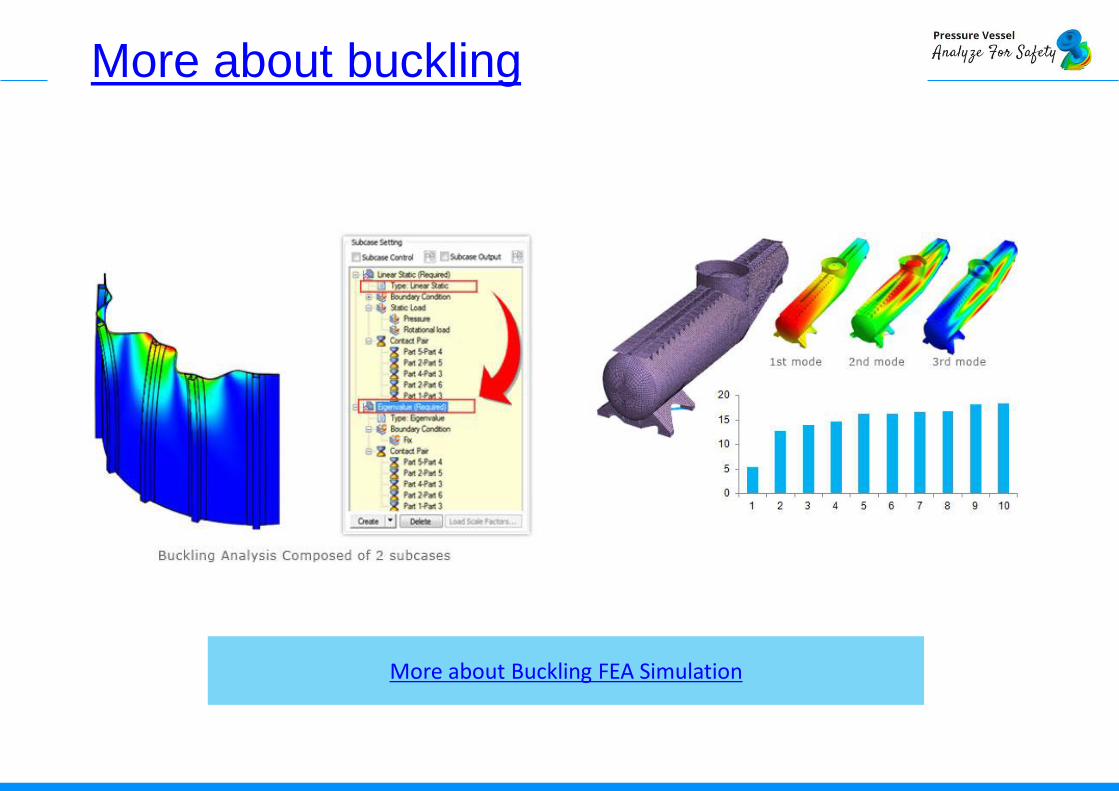
More about buckling

More about Buckling FEA Simulation