LINEAR VECTOR ERROR CORRECTION MODEL …web.usm.my/journal/aamjaf/vol 10-1-2014/AAMJAF 10-1... · the 2008 Global Economic Crisis are depressions examples of ... The regime switching

AAMJAF, Vol. 10, No. 1, 133–149, 2014

© Asian Academy of Management and Penerbit Universiti Sains Malaysia, 2014

ASIAN ACADEMY of MANAGEMENT JOURNAL

of ACCOUNTING and FINANCE

LINEAR VECTOR ERROR CORRECTION MODEL VERSUS MARKOV SWITCHING VECTOR ERROR CORRECTION

MODEL TO INVESTIGATE STOCK MARKET BEHAVIOUR

Seuk-Wai Phoong1*, Mohd Tahir Ismail2 and Siok-Kun Sek3

1,2,3 School of Mathematical Sciences,

Universiti Sains Malaysia, 11800, Pulau Pinang, Malaysia

*Corresponding author: [email protected] ABSTRACT The stock market can reflect the economy of a country. The movement of the stock market index may imply the economic condition in general. The 1997 Asian Financial Crisis and the 2008 Global Economic Crisis are examples of share depressions that impacted countries’ inflation, unemployment rates and gross national product (GNP). This study investigates how oil and gold prices impact the stock exchange using a linear vector error correction model (VECM) and a Markov switching vector error correction model (MS-VECM). The results show that oil and gold prices affect the stock market returns for the four selected countries, namely Malaysia, Singapore, Thailand and Indonesia. The MS-VECM is able to capture every change in the transition probabilities of the financial time series data and is more reliable than the linear VECM for examining the effect of oil and gold prices on the stock market. Keywords: vector error correction model, Markov switching model, stock market, oil price, gold price INTRODUCTION A stock market is a public entity and is an important component of the capital market that is used to execute various functions and services for investors and for the trading of companies. A stock market is also an investment intermediary that facilitates the economic and industrial development of a country. Oil, which is the most important limited resource, and gold, a common precious metal for jewellery and a popular investment commodity, are also included in this study to examine their effect on stock market changes.

Historical evidence shows that an increase in oil prices leads to higher taxes and therefore causes a decline in economic activities, thereby having a detrimental effect on the stock market. Jones and Kaul (1996) revealed that oil

Seuk-Wai Phoong, Mohd Tahir Ismail and Siok-Kun Sek

134

price has a significant negative effect on the stock markets of the United States, the United Kingdom, Japan and Canada during the post war period.

In addition, Papapetrou (2001), and Basher and Sadorsky (2006) verified

the importance of oil prices on changes in the stock market because higher production costs dampen cash flows. This effect may indirectly cause a decline in stock prices because an increase in oil prices is always related to inflationary pressures. These pressures, in turn, may have a detrimental effect by causing an increase in interest rates due to the control of the central bank. The growth of interest rates then leads to a fall in the stock market because higher interest rates make bonds look more attractive than stocks. In addition, although oil producers earn more money when the oil price is higher, more companies worldwide consume oil than produce oil; thus, a negative relationship is reported between oil prices and the stock market index.

Gold is a popular investment commodity. Gold is also included in this

paper to capture its effect on stock market returns in Malaysia, Singapore, Thailand and Indonesia. The linear vector error correction model (VECM) and the Markov switching vector error correction model (MS-VECM) are applied to examine the financial relationship between these variables. The performance of the VECM and the MS-VECM are compared so that the greatest significance and the most reliable outputs are obtained. Researchers such as Hache and Lantz (2011), Bilgili, Tuluce and Dogan (2012), and Miao, Wu and Su (2013) encounter problems such as structural changes, missing data and jumps or breaks when analysing financial data. Thus, a linear statistical method and a regime switching model are applied in this study to capture the transition of time series.

Applying the linear and regime switching models, this study seeks to

investigate the relationship between three variables, as mentioned above: stock market returns, oil price and gold price. We focus the analyses on four countries, namely Indonesia, Malaysia, Singapore and Thailand. Comparing the results from these two models, our results reveal that the oil price has a negative impact on the stock market while the gold price has a positive relationship with changes in the stock market.

This study contributes to the literature on stock market analyses in two

ways. First, our results provide an understanding of the dynamic effects of oil and gold prices on the stock exchange in four emerging markets by considering the impacts of the financial crisis. The regime switching model enables a more accurate interpretation of the impacts of financial crisis shocks on the stock exchange. Second, a comparison of the results from both the linear and the regime switching models provides robustness evaluations of the results obtained.

Linear VECM Versus MS-VECM to Investigate Stock Market

135

LINEAR VECM AND MARKOV SWITCHING VECM The stationary linear combination with integrated order zero is known as cointegrated. Cointegrating relationships between variables are always shown in macroeconomic time series models because the profit of firms should be proportional to the investment in a long-run equilibrium as documented in the theory of competitive markets. Thus, the VECM and MS-VECM, which are able to estimate the cointegrated structure variable and capture the long-run relationship of the variables in the financial model, are proposed to capture the transition of the time series in the model (Lütkepohl & Kratzig, 2004; Lütkepohl 2005). Although the VECM is an alternative to the vector autoregression (VAR) model for estimating cointegrating relationships with the first-differenced variables and the error correction term to be estimated, it has its limitations: for example, variance and covariance in the VECM are assumed to be constant, and this might influence the reliability of the result. In addition, the VECM has similar characteristics to the VAR model. It is sensitive to the presence of autocorrelation when choosing the number of lags in the model. Thus, the MS-VECM is included in this paper to compare the performances between the models so that the most reliable, valid and significant findings are obtained. The simple VECM with one integrated order, I(1), is written as

( ) ( )( ) ( )

1

11

p

t t t t k t k tk

y v s s y yα β ε−

− −=

∆ = + + Γ ∆ +∑ (1)

( )( )∑ tt sdii ,0..~ε

where ty∆ is a (M × 1) vector of differenced variable, v(st) is an unobservable

regime indicator variable; { }1,...,ts N∈ ; ( )tsα is a (M × r) matrix of adjustment parameters; β is the (M × r) matrix of long-run parameters (cointegrating vectors) with one period lags;

tε is error term and the error

covariance matrix is assumed to be constant (M = number of variables, r = number of parameters). The intercept, v, is a function with the underlying state mentioned as follows:


136

( )

1 if 1...

if

t

t

t s

N t

v s

v s v

v s N

== =

=

and it can be decomposed into

( ) ( ) ( ) ( ) ( )( ) ( )

1 1' ' ' '

=t t t

t t

v s v s v s

s s

β α β α α β α β

β δ αµ

− −

⊥ ⊥ ⊥ ⊥

∗⊥

= +

+ (2)

where ' 0α α⊥ = , ' 0β β⊥ = when α⊥ and β⊥ are ( )M M r× − matrices.

( )tsδ is ( )M r− linearly independent but state dependent drift and µ(st) is

mean of regime indicator. If each regime is characterised by a particular attractor in the system, the process can be written as:

( ) ( )( ) ( )1

11

δ α β µ δ ε−

− −=

∆ − = − + Γ ∆ − + ∑p

t t t t k t k t tk

y s y s y s

( )( )~ . . 0,t t

i i d Sε ∑ (3)

If the changes in ( )tv s are due to a small number of deterministic shifts, which is a common approach in the empirical modelling of financial time series, then it can be captured by including a set of dummy variables in the model. If regime switching is stochastic rather than deterministic, this may provide a biased or inefficient result.

In the MS-VECM framework, the MS-VECM model allows the shocks to each variable in the model to affect the transition probabilities of the phase shifting. The model also accounts for temporary periods that diverge from the long-run relationship. Thus, the MS-VECM plays an important role in capturing the long-run properties of the system.

Moreover, the MS-VECM model proposed by Krolzig (1997) acts as an

error correction mechanism in each disequilibrium regime because the regimes are generated by a stationary, irreducible Markov chain. Errors arising from regime shifts can be corrected towards the stationary distribution of the regimes by the MS-VECM.


137

The transition probabilities, pij (i and j is number of regimes) for the two regime generating process with 2

1j=∑ 1ijp i= ∀ , { }1,2j∈ can be summarised in the following matrix:

11 12

21 22

p pp p

Ρ =

(4) If 0 < r <n is the cointegration relationship among variables, ( )1∏ is a reduced

rank, r, and can be expressed as a two (m x r) matrices product and ( ) '1 αβ∏ = ,

where 'tyβ is a cointegrating vector that is a stationary linear combination of the

I(1) variables and α is the factor loading matrix. The unobserved state of ξ

with ( ) 1tI s i= = is st = i and zero otherwise. The system can be presented by the following matrix:

( )( )1

12

t

t

I sI s

ξ =

= = (5)

The MS-VECM equation can be denoted as

( )*1 1t t t t ty N L y zξ α ε− −∆ = +∏ ∆ + + , where [ ]1 2N v v= , ξt is parameter,

( )* L∏ is predicted likelihood parameter, 't tz yβ= and

tε is error term.

The density vectors of the observed time series vector yt conditional on past information, Yt–1 and tξ , are:

( )( )

( )( )

1 1 1 1 1

1 2 2 1 2

; , ;

; , ;t t t t t

tt t t t t

P y Y P y t Y

P y Y P y t Y

λ ξ λη

λ ξ λ− −

− −

== =

= (6)

where λ is the parameter vector in the regime. Conditional on the cointegration matrix, the likelihood function model is:


138

( ) ( ) ( )( ) ( ) ( )

( ) ( )

( ) ( )

11

11

,

, ,

, , ,

, ,

λ

λ

θ θ ξ θ ξ

θ ξ θ ξ ρ ξ ξ

ξ θ ξ λ

ξ ρ ξ ξ ξ ρ

−=

−=

= =

= ×

= ∆

=

∫∫

∏

∏

T T T

T T

T

T t t ttT

t tt

L Y P Y P Y d

L Y P Y P d

P y P y Y

P P (7)

where the parameter vector θ consists of the parameter vector λ and ρ is the parameter vector. The Expectation-Maximisation (EM) algorithm is also used to estimate the MS-VECM, including the log-likelihood results. In VECM analysis, a stationary test is vital as a pre-test before implementing the statistical model, VECM. The stationary tests, the Augmented Dickey Fuller (ADF) and Kwiatkowski-Philips-Schmidt-Shin (KPSS) tests, are applied before conducting the analysis. If the variables in the system are non-stationary, we need to transform the series to a stationary series through a differencing process. It is then concluded that the series have a unit root in the system and ordinary regression analyses are not suitable to estimate the relationships between the set of variables in the system. In this case, the VECM is applied to analyse the relationships between variables; the variables are also known as cointegration variables. This study involves 5 steps of analysis before VECM is applied. The first step of the research design is to undergo a stationary test; the second step is to decide the number of variables in the model; the third step is to transform the data to log form and the fourth step is to decide the number for the lag length. Although there are many approaches that are able to model the VECM, such as determining the number of lags in the error correction term, but they generally follow the same order as the VAR. The next step is to decide whether we want to include deterministic terms such as dummies, trends and seasonal terms in the model. This step is important prior to starting to model the financial relationship using VECM because deterministic terms may have some properties of the variables. These modelling strategies are same with the MS-VECM; they have been involved in the stationary test, the cointegration test and finally employed in the MS-VECM to capture the oil and gold price effects on the stock market index.


139

MODEL COMPARISONS Several information criterion tests are used in this paper to compare the estimates from the linear VECM and the MS-VECM for the oil and gold price effects on stock market behaviour. The Akaike Information Criterion (AIC) Test, the Schwarz Information Criterion (SC) Test, the Hannan-Quinn Information Criterion (HQ) Test and the Log-likelihood Ratio Test are applied to determine the best statistical model for capturing the time series data. The formulae of the information tests are:

AIC = 2p – 2log(L) SC = pln(n)-2log(L)

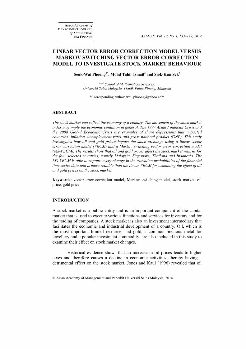
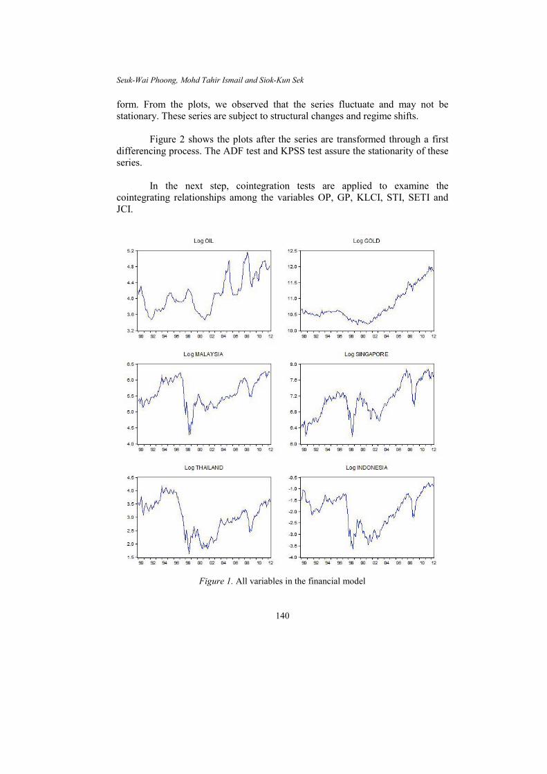
HQ = 2plnln(n)-2ln(L). Likelihood ratio test: D = 2ln(L1) – 2ln(L0) where p represents the number of parameters, n is the number of observations and L is the maximised likelihood value. The AIC test is applied because it is a goodness of fit test for the estimated statistical model. Moreover, the AIC test is a powerful tool for asymptotically estimating the higher lag structure of the time series model. The SC test is a measurement test for model selection to estimate the efficiency of the parametric model, and the HQ test consistently estimates the order of the financial model. In addition, the log-likelihood test is also used in this study to compare the model performance of the linear VECM and the MS-VECM in the data fit. RESULTS AND DISCUSSION The monthly index data is obtained from DATASTREAM (Thomson Reuters. Boston, USA). The data range is from December 1989 until May 2012, which provides a total of 270 observations. The dataset are transformed into natural logs to linearise the system or to simplify the data analysis due to the independent properties of units. Moreover, the computed outputs may have many decimal places; therefore, natural logs are taken in the data to avoid cutting off the last few decimal places and thus obtain a more significant result. Figure 1 shows the plot for oil price (OP), gold price (GP), the Malaysia stock market index (KLCI), the Singapore stock market index (STI), the Thailand stock market index (SETI) and the Indonesia stock market index (JCI) in log


140

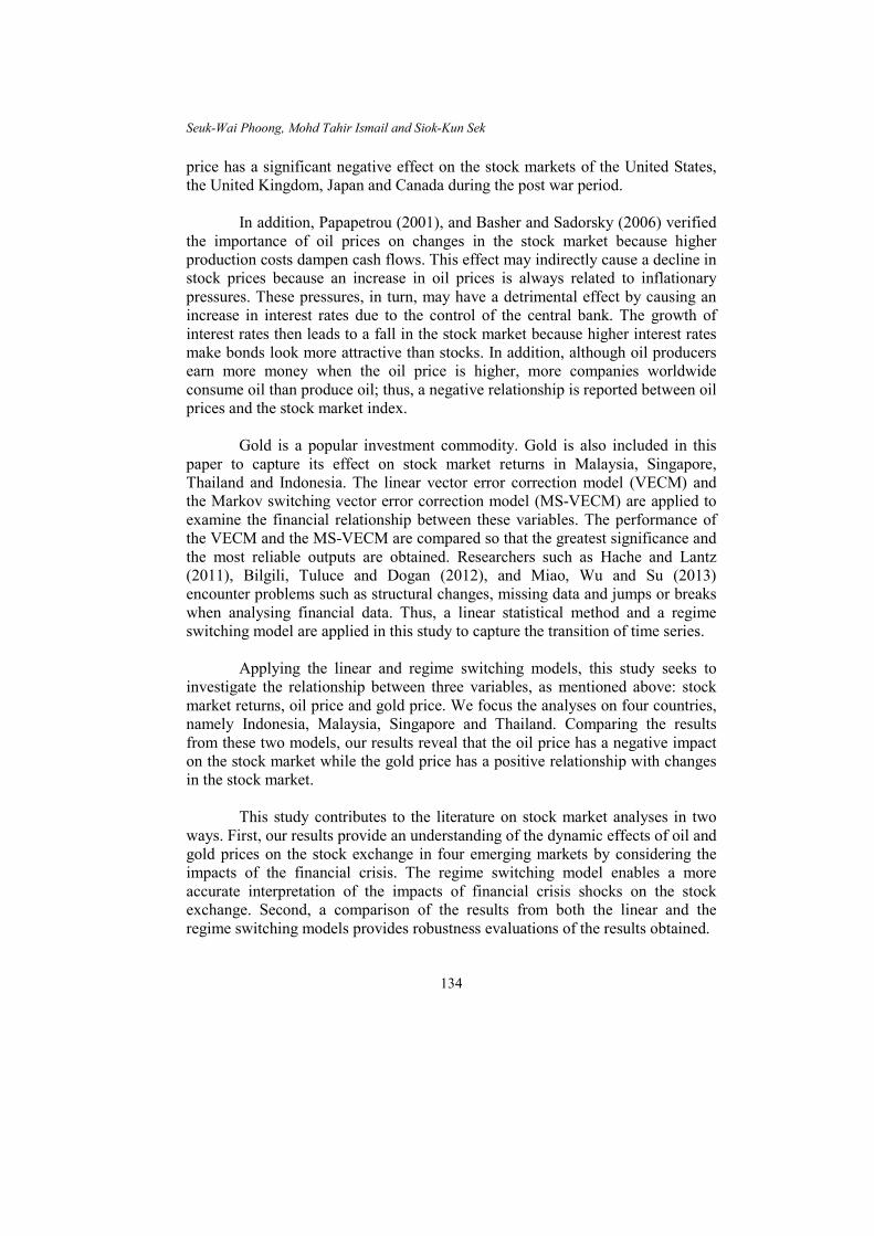
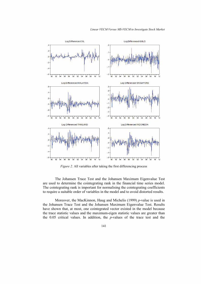
form. From the plots, we observed that the series fluctuate and may not be stationary. These series are subject to structural changes and regime shifts. Figure 2 shows the plots after the series are transformed through a first differencing process. The ADF test and KPSS test assure the stationarity of these series. In the next step, cointegration tests are applied to examine the cointegrating relationships among the variables OP, GP, KLCI, STI, SETI and JCI.

Figure 1. All variables in the financial model


141

Figure 2. All variables after taking the first differencing process

The Johansen Trace Test and the Johansen Maximum Eigenvalue Test are used to determine the cointegrating rank in the financial time series model. The cointegrating rank is important for normalising the cointegrating coefficients to require a suitable order of variables in the model and to avoid distorted results.

Moreover, the MacKinnon, Haug and Michelis (1999) p-value is used in the Johansen Trace Test and the Johansen Maximum Eigenvalue Test. Results have shown that, at most, one cointegrated vector existed in the model because the trace statistic values and the maximum-eigen statistic values are greater than the 0.05 critical values. In addition, the p-values of the trace test and the


142

maximum eigenvalue test in the hypothesis testing on at most one cointegrating equation are less than 0.05; thus, it can be concluded that there are two cointegrating relationships between the variables in the financial model at a 95% significant level.

Although the Johansen test (Table 1) has proven that two cointegrating

relationships exist between the parameters, it does not explain which variables are cointegrated. Thus, a further estimation of the variables in the model is reviewed. The submodels are partitioned according to the commodity price because this study focuses on how the commodity price has affected stock market growth. Table 1 Johansen test outputs

Series Hypothesis on no. of CE Eigenvalue Trace statistic Maximum-

Eigen statistic

OP, GP, KLCI, STI, SETI and JCI

None 0.199733 136.2312* 58.59890* At most 1 0.146872 77.63227* 41.77642* At most 2 0.077311 35.85586 21.16182 At most 3 0.040511 14.69403 10.87633 At most 4 0.013663 3.817706 3.618207 At most 5 0.000758 0.199500 0.199500

0.05 critical value

None At most 1

At most 2

At most 3

At most 4

At most 5

Trace statistic 83.93712 60.06141 40.17493 24.27596 12.32090 4.129906 Maximum-Eigen statistic 36.63019 30.43961 24.15921 17.79730 11.22480 4.129906

Notes: * denotes rejection of the hypothesis at the 0.05 level. CE – cointegrating equation.

The lag order for the tests shown in Table 2 is selected based on the results of the VAR lag order information criterion selection test. Because the GP and STI, GP and SETI, and GO and JCI series rejected the null hypothesis at a 95% significance level, there are two cointegrating relationships existing between these series.

GP with STI, GP with SETI, and GP with JCI rejected the null

hypothesis. Therefore, these variables are tested again using r = 1, recording that these series rejected the null hypothesis when one cointegrating relationship existed in the system. Furthermore, the results have shown that the relationship


143

between GP and JCI rejected the null hypothesis when r = 1. Thus, we concluded that GP and JCI are cointegrated. Changes in the gold price impact changes in Indonesia’s stock market. Therefore, the two regime mean adjusted heteroskedasticity of the Markov switching vector error correction model in the first autoregressive order [MSMH(2)-VECM(1)] is used in this study.

Table 2 Johansen cointegration tests of OP, KLCI, STI, SETI and JCI

Series Hypothesis on no. of CE Eigenvalue Trace statistic Maximum-Eigen statistic

OP and KLCI

None 0.032731 8.858093 8.852114 At most 1 2.25E-05 0.005979 0.005979

OP and STI None 0.059475 16.37170 16.37161

At most 1 3.26E-07 8.71E-05 8.71E-05

OP and SETI None 0.011707 3.334527 3.144317

At most 1 0.000712 0.190210 0.190210

OP and JCI None 0.022854 6.253878 6.172930

At most 1 0.000303 0.080949 0.080949

GP and KLCI

None 0.030955 11.18557 8.364224 At most 1 0.010550 2.821341 2.821341

GP and STI None 0.038943 12.60890* 10.4863

At most 1 0.008008 2.122505 2.122505

GP and SETI None 0.108765 31.45933* 29.36256*

At most 1 0.008189 2.096769 2.096769

GP and JCI None 0.051384 21.29932* 14.08453*

At most 1 0.026660 7.214790* 7.214790*

0.05 critical value None At most 1

Trace statistic 12.32090 4.129906 Maximum-Eigen statistic 11.22480 4.129906

Notes:* denotes rejection of the hypothesis at the 0.05 level. CE – cointegrating equation.

Figure 1 shows that all variables in the financial model experience

structural change and exhibit non-stationary properties. Therefore, the mean adjusted MS-VECM model is used to capture the transition of the series. The reasons for choosing the mean varying factor is that the mean value can be adjusted to a new level after a translation from one state to another. Thus, the


144

mean adjustment of MS-VECM is selected to explain the relationship of the financial model. The results are shown in the following table.

The likelihood ratio test of the Markov switching-mean-heteroskedasticity (MSMH)-VECM is 2(27) 362.1067,χ = indicating that the model has no misspecification problem. The first regime (st = 1) in MSMH(2)-VECM(1) represented the recession state, and the second regime (st = 2) represented the growth state. The regimes are classified based on the accumulation of the decreasing periods of the oil price, the gold price and the stock index in the first regime and the increasing periods of the oil price, the gold price and the stock index in the second regime.

OP and GP in MSMH(2)-VECM(1) reported positive coefficients in both

regimes. This result indicated that the oil price is increasing during the recessionary periods of these four countries’ stock markets. The same conclusion is reported in the study of Sauter and Awerbuch (2003). The gold price presented a higher increasing rate on regime 2. Moreover, although the demand for gold increased in the recessionary period, there is greater demand for gold during the growth period.

All of the variables in the MSMH-VECM reported high volatility and a

positive mean in regimes 1 and 2. Thus, it can be concluded that these findings are reliable and significant because these results is closer to the mean.

The transition probabilities of the MSMH(2)-VECM(1) are:

=

0.7230 0.2770P

0.1186 0.8814

which means that the transition probability from state 1 to state 2 is 0.2770 and from state 2 to state 1 is 0.1186. Regime 2 has higher probability than regime 1. According to Table 3, regime 2 is more prevalent than regime 1 in this case. Moreover, 70% of the time series data are reported in regime 2, which also supports that regime 2 is the dominant state in the model and represents an asymmetric business cycle.

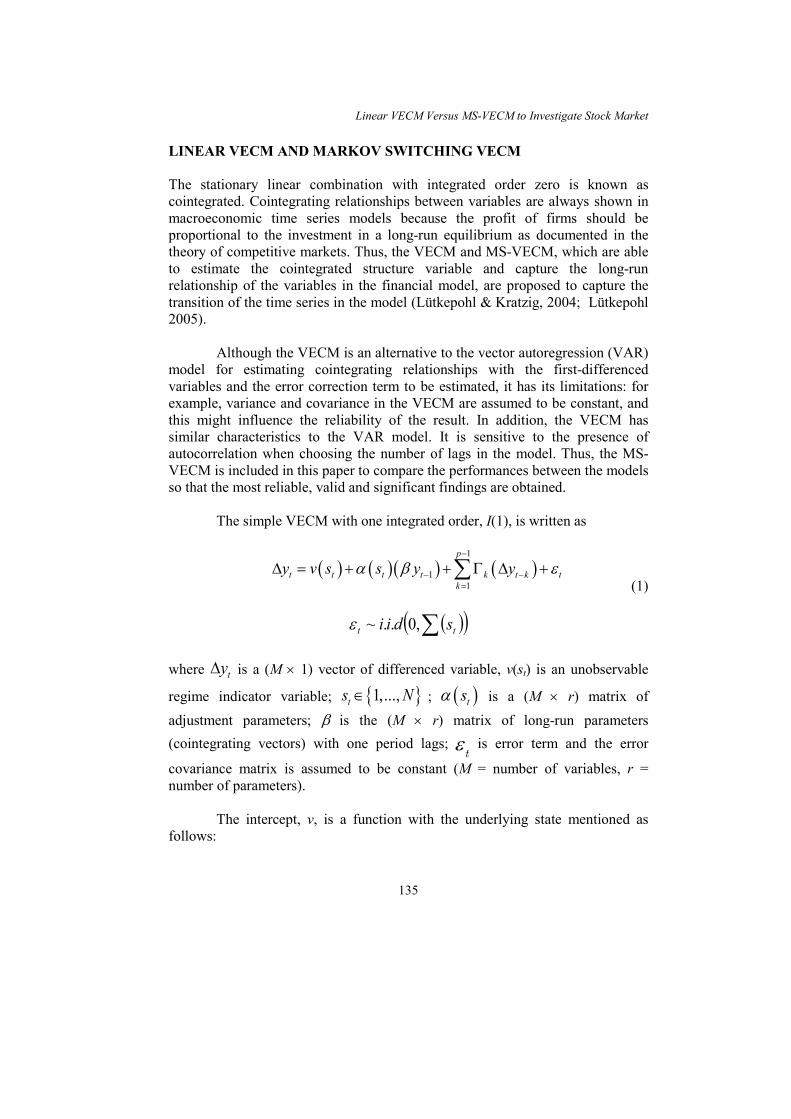
The first panel in Figure 3 is sketched to explain how the inferred regime

probabilities switched into the mean growth rate, while the second panel is sketched based on the filtered and smoothed probabilities of regime 1. The third panel shows the filtered and smoothed probabilities of regime 2. The filtered and


145

smoothed probabilities present the optimal inference for the turning point and the state during the recession and growth states.

Table 3 MSMH(2)-VECM(1) outputs

Likelihood ratio test

362.1067 DAVIES p-value = [0.0000] *

OP GP KLCI STI SETI JCI µ (st = 1) 0.008156 0.001875 –0.006682 –0.005297 –0.007627 –0.016678 µ (st = 2) 0.002874 0.006141 0.010253 0.010692 0.006512 0.013381 OPt–1 0.271736 –0.057184 –0.114802 –0.135848 –0.113235 –0.112578 GPt–1 0.088358 –0.155105 –0.103469 –0.050447 0.024585 0.108350

(st = 1) 0.096728 0.058073 0.132387 0.122057 0.149247 0.173702

(st = 2) 0.039393 0.035457 0.046797 0.044749 0.07452 0.066677 Matrix of transition probabilities, pij

st = 1 st = 2 st = 1 0.7230 0.2770 st = 2 0.1186 0.8814

Regime properties No. of observations Probability Duration

st = 1 81.4 0.2997 3.61 st = 2 186.6 0.7003 8.44

Note: * indicates that the p-value is significant at the 5% level.

Figure 3. MSMH(2)-VECM(1) probabilities sketched


146

The smoothed and filtered probabilities in MSMH(2)-VECM(1) exhibit many structural changes during the period from December 1989 until May 2012. Long recessionary periods, including July 1997 until January 1999 and April 1999 until June 2000, are detected when estimating the MSMH-VECM. The short depression periods included February 1990 until May 1990, July 1990 until February 1991, December 1993 until January 1994, March 2001 until September 2001, October 2002, September 2008 until October 2008 and March 2009 until May 2009; these are also presented in the output of MSMH(2)-VECM(1) in the analysis of the relationship model for OP, GP, KLCI, STI, SETI and JCI. This result indicates that MSMH(2)-VECM(1) is able to capture every change in the data series whether it is a short period or a long period shift.

MS-VECM is able to capture every single change of the transition

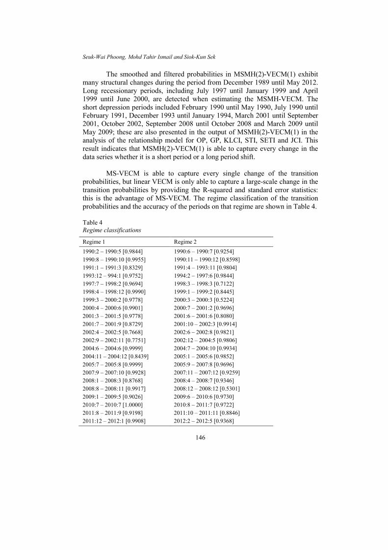
probabilities, but linear VECM is only able to capture a large-scale change in the transition probabilities by providing the R-squared and standard error statistics: this is the advantage of MS-VECM. The regime classification of the transition probabilities and the accuracy of the periods on that regime are shown in Table 4.

Table 4 Regime classifications

Regime 1 Regime 2

1990:2 – 1990:5 [0.9844] 1990:8 – 1990:10 [0.9955] 1991:1 – 1991:3 [0.8329] 1993:12 – 994:1 [0.9752] 1997:7 – 1998:2 [0.9694] 1998:4 – 1998:12 [0.9990] 1999:3 – 2000:2 [0.9778] 2000:4 – 2000:6 [0.9901] 2001:3 – 2001:5 [0.9778] 2001:7 – 2001:9 [0.8729] 2002:4 – 2002:5 [0.7668] 2002:9 – 2002:11 [0.7751] 2004:6 – 2004:6 [0.9999] 2004:11 – 2004:12 [0.8439] 2005:7 – 2005:8 [0.9999] 2007:9 – 2007:10 [0.9928] 2008:1 – 2008:3 [0.8768] 2008:8 – 2008:11 [0.9917] 2009:1 – 2009:5 [0.9026] 2010:7 – 2010:7 [1.0000] 2011:8 – 2011:9 [0.9198] 2011:12 – 2012:1 [0.9908]

1990:6 – 1990:7 [0.9254] 1990:11 – 1990:12 [0.8598] 1991:4 – 1993:11 [0.9804] 1994:2 – 1997:6 [0.9844] 1998:3 – 1998:3 [0.7122] 1999:1 – 1999:2 [0.8445] 2000:3 – 2000:3 [0.5224] 2000:7 – 2001:2 [0.9696] 2001:6 – 2001:6 [0.8080] 2001:10 – 2002:3 [0.9914] 2002:6 – 2002:8 [0.9821] 2002:12 – 2004:5 [0.9806] 2004:7 – 2004:10 [0.9934] 2005:1 – 2005:6 [0.9852] 2005:9 – 2007:8 [0.9696] 2007:11 – 2007:12 [0.9259] 2008:4 – 2008:7 [0.9346] 2008:12 – 2008:12 [0.5301] 2009:6 – 2010:6 [0.9730] 2010:8 – 2011:7 [0.9722] 2011:10 – 2011:11 [0.8846] 2012:2 – 2012:5 [0.9368]


147

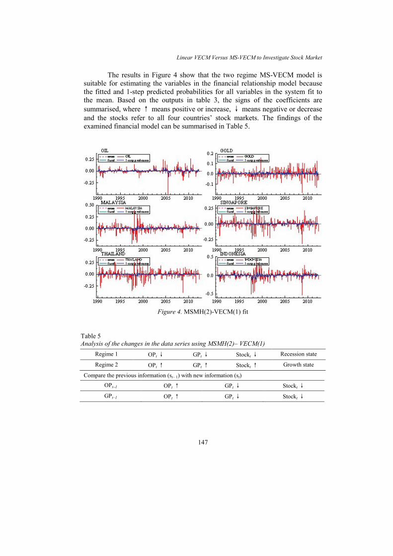
The results in Figure 4 show that the two regime MS-VECM model is suitable for estimating the variables in the financial relationship model because the fitted and 1-step predicted probabilities for all variables in the system fit to the mean. Based on the outputs in table 3, the signs of the coefficients are summarised, where ↑ means positive or increase, ↓ means negative or decrease and the stocks refer to all four countries’ stock markets. The findings of the examined financial model can be summarised in Table 5.

Figure 4. MSMH(2)-VECM(1) fit

Table 5 Analysis of the changes in the data series using MSMH(2)– VECM(1)

Regime 1 OPt ↓ GPt ↓ Stockt ↓ Recession state

Regime 2 OPt ↑ GPt ↑ Stockt ↑ Growth state

Compare the previous information (st– 1) with new information (st)

OPt–1 OPt ↑ GPt ↓ Stockt ↓

GPt–1 OPt ↑ GPt ↓ Stockt ↓


148

Therefore, it can be concluded that an increase in oil price leads to a decline in the stock index, and a rise in the gold price impacts the growth of the stock market. Table 6 reported the findings of the log-likelihood test and the information criterion tests, as discussed in the previous section.

Table 6 Criterion test results on the Markov switching models

Criterion tests Linear VECM MSMH– VECM

Log– likelihood 2138.44 2319.49* AIC –15.49 –16.62* HQ –15.15 –16.13* SC –14.64 –15.39*

Note: * indicates better performance for the model. It is observed that the value of the log– likelihood, AIC, HQ and SC tests between the linear VECM and MSMH-VECM are very close to each other. These values are close because the MS-VECM is derived from the VECM by adding more features to the equation. The small value of the information criterion test statistics means that the model is able to fit the data well and provide more reliable and valid results. Thus, the MSMH-VECM performs better than linear VECM based on the information criterion and log– likelihood ratio statistics.

CONCLUSION Linear VECM and MS-VECM are used in this paper to examine the financial relationship between oil prices and the stock exchange. Comparisons between these two statistical models are made to determine the best model. The results show that a decrease in the oil price will lead to an increase of the stock market index. This condition is related to tax adjustment. Higher oil prices may lead to higher taxes because the side products of oil become more expensive. Higher taxes and more expensive products indicates lower investment because people have less money to invest, and hence a lower stock index will be observed.

In addition, the gold price is reported to have a positive relationship with stock returns: an increase in the gold price will lead to higher stock returns. This result can be related to the demand for precious metals for investment and also for practical use such as jewellery, medicine, food or as a store for value. In addition, historical evidence has proved that during the Asian Financial Crisis in 1997, the government of Thailand advised its residents to sell gold. Thus, oil and gold prices are factors influencing changes in the stock markets.


149

ACKNOWLEDGEMENT This research was sponsored by the Universiti Sains Malaysia Short term grant (304/PMATHS/6313045). REFERENCES Basher, S. A., & Sadorsky, P. (2006). Oil price risk and emerging stock markets. Global

Finance Journal, 17, 224–251. Bilgili, F., Tuluce, N. S. H., & Dogan, I. (2012). The determinants of FDI in Turkey: A

Markov regime– switching approach. Economic Modelling, 29(4), 1161–1169. Hache, E., & Lantz, F. (2011). Oil price volatility: An econometric analysis of the WTI

market (pp. 228–232). France: IFP Energies Nouvelles, Centre Économie et Gestion, Napoléon Bonaparte.

Johansen, S. (1991). Estimating and testing cointegration vectors in Gaussian vector autoregressive models. Econometrica, 59, 1551–1580.

Jones, C. M., & Kaul, G. (1996). Oil and the stock markets. The Journal of Finance, 51(2), 463–491.

Krolzig, H. M. (1997). Markov-switching vector autoregression. Berlin: Springer. Lütkepohl, H., & Kratzig, M. (2004). Applied time series econometrics. Berlin: The Press

Syndicate of the University of Cambridge. Lütkepohl, H. (2005). New introduction to multiple time series analysis. Berlin: Springer. MacKinnon, J. G., Haug, A. A., and Michelis, L. (1999). Numerical distribution functions

of likelihood ratio tests for cointegration. Journal of Applied Econometrics, 14(5), 563–577.

Miao, D. W. C., Wu, C. C., & Su, Y. K. (2013). Regime-switching in volatility and correlation structure using range-based models with Markov-switching. Economic Modelling, 31(C), 87–93.

Papapetrou, E. (2001). Oil price shocks, stock market, economic activity and employment in Greece. Energy Economics, 23(5), 511–532.

Sauter, R., & Awerbuch, S. (2003). Oil price volatility and economic activity: A survey and literature review. Paris: International Energy Agency (IEA). Retrieved 29 July 2013, from https://www.google.com.my/url?sa=t&rct=j&q=&esrc=s& source=web&cd=1&cad=rja&uact=8&ved=0CBsQFjAA&url=http%3A%2F%2Fwww.awerbuch.com%2Fshimonpages%2Fshimondocs%2FOil-price-Volatility -03.doc&ei=eVyU4v2OtCWuASCwYCICg&usg=AFQjCNGn2PpWPEjOP6t yoan0sfpZ5_HK-g&bvm=bv.70138588,d.c2E

Documents

LINEAR VECTOR ERROR CORRECTION MODEL …web.usm.my/journal/aamjaf/vol 10-1-2014/AAMJAF 10-1... · the 2008 Global Economic Crisis are depressions examples of ... The regime switching