Linear-time recognition of circular-arc graphs

Ross M. McConnell ∗

Abstract

A graph G is a circular-arc graph if it is the intersection graph of a set of arcs on acircle. That is, there is one arc for each vertex of G, and two vertices are adjacent inG if and only if the corresponding arcs intersect. We give a linear-time algorithm forrecognizing this class of graphs. When G is a member of the class, the algorithm givesa certificate in the form of a set of arcs that realize it.

∗Department of Computer Science, Colorado State University, Fort Collins, CO 80523-1873 USA,rmm@cs.colostate.edu. This research was supported by the University of Metz. The author gratefullyacknowledges Dieter Kratsch for extensive inputs to this paper, and the anonymous referees for many help-ful comments and observations.

1

a

b

c

d

e

f

a

b c

d

e

f

a

b c d gf

e

a

b c

d e

f g

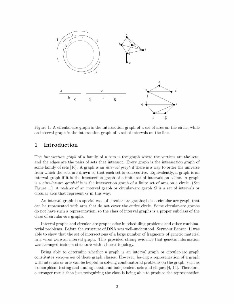
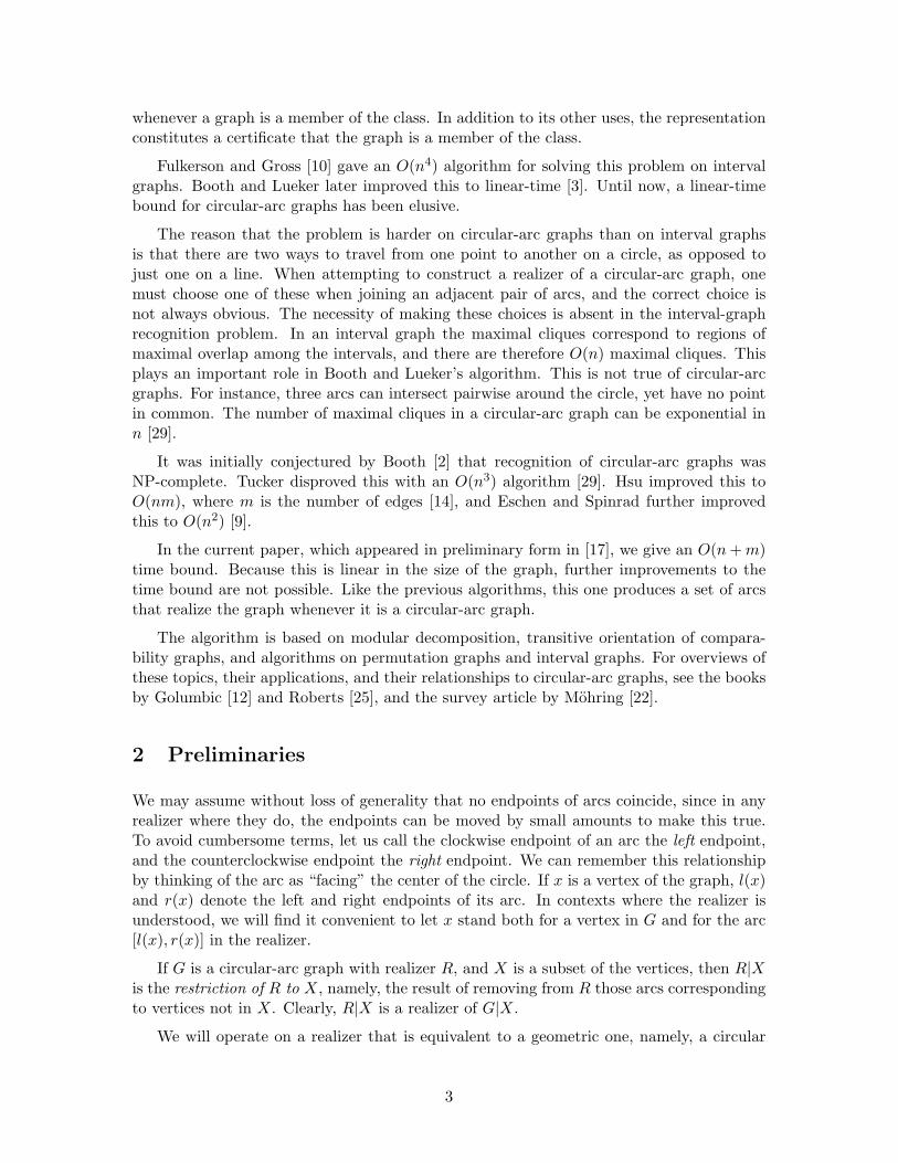
Figure 1: A circular-arc graph is the intersection graph of a set of arcs on the circle, whilean interval graph is the intersection graph of a set of intervals on the line.

1 Introduction

The intersection graph of a family of n sets is the graph where the vertices are the sets,and the edges are the pairs of sets that intersect. Every graph is the intersection graph ofsome family of sets [16]. A graph is an interval graph if there is a way to order the universefrom which the sets are drawn so that each set is consecutive. Equivalently, a graph is aninterval graph if it is the intersection graph of a finite set of intervals on a line. A graphis a circular-arc graph if it is the intersection graph of a finite set of arcs on a circle. (SeeFigure 1.) A realizer of an interval graph or circular-arc graph G is a set of intervals orcircular arcs that represent G in this way.

An interval graph is a special case of circular-arc graphs; it is a circular-arc graph thatcan be represented with arcs that do not cover the entire circle. Some circular-arc graphsdo not have such a representation, so the class of interval graphs is a proper subclass of theclass of circular-arc graphs.

Interval graphs and circular-arc graphs arise in scheduling problems and other combina-torial problems. Before the structure of DNA was well-understood, Seymour Benzer [1] wasable to show that the set of intersections of a large number of fragments of genetic materialin a virus were an interval graph. This provided strong evidence that genetic informationwas arranged inside a structure with a linear topology.

Being able to determine whether a graph is an interval graph or circular-arc graphconstitutes recognition of these graph classes. However, having a representation of a graphwith intervals or arcs can be helpful in solving combinatorial problems on the graph, such asisomorphism testing and finding maximum independent sets and cliques [4, 14]. Therefore,a stronger result than just recognizing the class is being able to produce the representation

2

whenever a graph is a member of the class. In addition to its other uses, the representationconstitutes a certificate that the graph is a member of the class.

Fulkerson and Gross [10] gave an O(n4) algorithm for solving this problem on intervalgraphs. Booth and Lueker later improved this to linear-time [3]. Until now, a linear-timebound for circular-arc graphs has been elusive.

The reason that the problem is harder on circular-arc graphs than on interval graphsis that there are two ways to travel from one point to another on a circle, as opposed tojust one on a line. When attempting to construct a realizer of a circular-arc graph, onemust choose one of these when joining an adjacent pair of arcs, and the correct choice isnot always obvious. The necessity of making these choices is absent in the interval-graphrecognition problem. In an interval graph the maximal cliques correspond to regions ofmaximal overlap among the intervals, and there are therefore O(n) maximal cliques. Thisplays an important role in Booth and Lueker’s algorithm. This is not true of circular-arcgraphs. For instance, three arcs can intersect pairwise around the circle, yet have no pointin common. The number of maximal cliques in a circular-arc graph can be exponential inn [29].

It was initially conjectured by Booth [2] that recognition of circular-arc graphs wasNP-complete. Tucker disproved this with an O(n3) algorithm [29]. Hsu improved this toO(nm), where m is the number of edges [14], and Eschen and Spinrad further improvedthis to O(n2) [9].

In the current paper, which appeared in preliminary form in [17], we give an O(n + m)time bound. Because this is linear in the size of the graph, further improvements to thetime bound are not possible. Like the previous algorithms, this one produces a set of arcsthat realize the graph whenever it is a circular-arc graph.

The algorithm is based on modular decomposition, transitive orientation of compara-bility graphs, and algorithms on permutation graphs and interval graphs. For overviews ofthese topics, their applications, and their relationships to circular-arc graphs, see the booksby Golumbic [12] and Roberts [25], and the survey article by Mohring [22].

2 Preliminaries

We may assume without loss of generality that no endpoints of arcs coincide, since in anyrealizer where they do, the endpoints can be moved by small amounts to make this true.To avoid cumbersome terms, let us call the clockwise endpoint of an arc the left endpoint,and the counterclockwise endpoint the right endpoint. We can remember this relationshipby thinking of the arc as “facing” the center of the circle. If x is a vertex of the graph, l(x)and r(x) denote the left and right endpoints of its arc. In contexts where the realizer isunderstood, we will find it convenient to let x stand both for a vertex in G and for the arc[l(x), r(x)] in the realizer.

If G is a circular-arc graph with realizer R, and X is a subset of the vertices, then R|Xis the restriction of R to X, namely, the result of removing from R those arcs correspondingto vertices not in X. Clearly, R|X is a realizer of G|X.

We will operate on a realizer that is equivalent to a geometric one, namely, a circular

3

ordering of l(x) : x ∈ V ∪ r(x) : x ∈ V . The circular ordering represents the orderof left and right endpoints as one travels counterclockwise around the circle. The circularordering can be represented by an ordered list, where an incremental rightward movementis a movement from position i to position i + 1 (mod 2n). Let us call this the circular-listrepresentation of the realizer. A circular-arc graph may have more than one realizer; whencounting its realizers, we consider two realizers to be the same if one is a cyclic permutationof the other, and different otherwise. If G is an interval graph, we adopt the convention ofcircularly permuting the realizer so that an uncovered part of the circle occurs immediatelyfollowing the last endpoint in the list. Let us call this the ordered list representation ofan interval realizer. We consider two sets of intervals to be equivalent if their ordered-listrepresentations are identical. Let the mirror transpose RT of a realizer be the result ofreversing the order of elements in the ordered list representation and reversing the roles ofleft and right endpoints.

Let G = (V,E) be a graph. By n(G) and m(G) we denote the number of vertices andedges, respectively, of G. We use n and m for these if G is understood. Let E′ ⊆ G denotethat E′ ⊆ E, and e ∈ G denote that e ∈ E. G denotes the complement of G, whose verticesare V and whose edges are the non-edges of G. If G is a digraph, GT denotes its transpose,which is obtained by reversing the directions of all of its directed edges. If v is a vertex inG, let N(G, v) denote the neighbors of v in G. When G is understood, we may use N(v)to denote this. N [G, v] denotes the closed neighborhood, N(G, v) ∪ v, and N [v] denotesthis when G is understood. Let N(G, v) denote the set V −N [G, v] of non-neighbors of v,and let N(v) denote the same thing when G is understood.

If A is a matrix, we let Aij denote the value in row i and column j of A. If X ⊆ V , G|Xdenotes the restriction of G to X, namely, the graph G′ = (X, E ∩ (X ×X)). Similarly, ifA is an n× n matrix and X is a subset of 1, 2, ..., n, then A|X is the |X| × |X| matrix ofentries whose rows and columns are both in X. An n×n matrix can be represented with adirected edge-labeled graph on n vertices numbered 1 through n. The label of the directededge from vertex i to vertex j is just the entry in row i and column j of the matrix. Wemay therefore refer to the vertices and edges of a matrix.

A transitive orientation of an undirected graph is an assignment of directions to itsedges so that the resulting digraph is a transitive dag. A graph is a comparability graph ifthere exists a transitive orientation of it. Finding a transitive orientation of a comparabilitygraph takes O(n + m) time [18]. The complement of an interval graph is a comparabilitygraph.

A permutation graph is a graph that is a comparability graph, and whose complementis also a comparability graph. The union of a transitive orientation of a permutation graphand a transitive orientation of its complement gives a linear order on the vertices. Reversingthe orientations in the complement and again taking the union of the two gives anotherlinear order. Two vertices are adjacent in the graph iff their relative order is the same inboth of these orderings. This permutation realizer gives a way to represent a permutationgraph with two orderings of the vertices.

4

3 Intersection matrices

If G is a circular-arc graph and R is a realizer, we can classify each ordered pair (x, y) ofvertices with x 6= y according to the type of intersection of their arcs in R, as follows [29,14, 9]:

• single overlap: Arc x contains a single endpoint of arc y.

• double overlap: x and y jointly cover the circle and each contains both endpointsof the other.

• Arc x is contained in arc y

• Arc x contains arc y

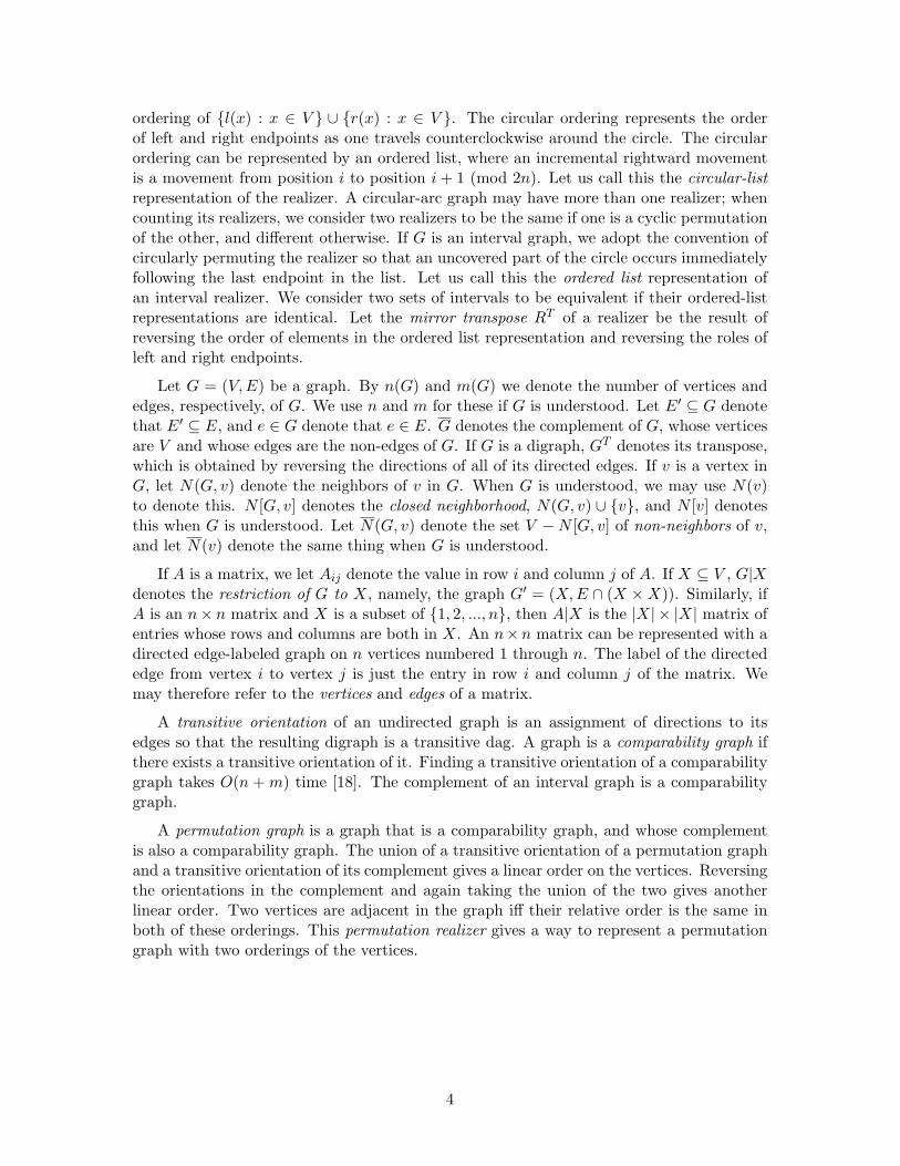
Let v1, v2, ..., vn be a numbering of vertices of V . A circular-arc matrix of a realizer Ris an n× n matrix T where Tij is a label that tells the type of the relationship between arcvi and arc vj in the realizer. (See Figure 2.) R is a realizer of T if it realizes not just thegraph implied by T but also the intersection types claimed by T . A circular-arc matrix isan interval matrix if there is a realizer for it that does not cover the circle; in this case G isan interval graph, since a circular-arc realizer can be cut at an uncovered point on the circleand rolled out onto a line. An intersection matrix is a matrix whose entries give the allegedintersection types in some circular-arc realizer, but where it is not a requirement that therealizer exist. In general, we refer to a circular-arc matrix as an intersection matrix, exceptwhen we wish to emphasize that a realizer is required to exist.

From these types, we get a partition of the complete graph into the following undirectedgraphs on V :

• G1: single overlaps

• G2: double overlaps

• Gc: containments

• Gn = G: non-intersections

We will use multiple subscripts to denote unions of these. For example G = G12c, theunion of edges of G1, G2, and Gc. An edge of Gc can be viewed as two directed edges withthe following classifications.

• Dc: edges of the form (x, y) : x is contained in y

• (Dc)T : edges of the form (x, y) : x contains y.

The non-neighbors of a vertex x are its neighbors in Gn, its overlap neighbors are itsneighbors in G1, its double-overlap neighbors are its neighbors in G2, and its containmentneighbors are its neighbors in Gc. G(T ) denotes the graph that gives the pairs that intersect,hence G(T ) = G12c. Its neighbors are the neighbors in G(T ).

5

ea f

dc

b

a b c d e fa t 1 2 n cb c 1 2 n c

c 1 1 c n 1d 2 2 t t 2e n n n c nf t t 1 2 n

Figure 2: The intersection matrix of a circular-arc realizer gives the types of intersectionsbetween arcs. The types consist of two arcs overlapping at one endpoint, G1 (1), two arcsoverlapping at two endpoints, G2 (2), two arcs not intersecting, Gn (n), one arc beingcontained in the other Dc (c) and one arc containing the other (Dc)T (t). The pairs ofeach type give the graphs G1, G2, Gn, Dc, and (Dc)T , respectively. The matrix has a skewsymmetry, where t in a row i, column j corresponds to c in row j column i.

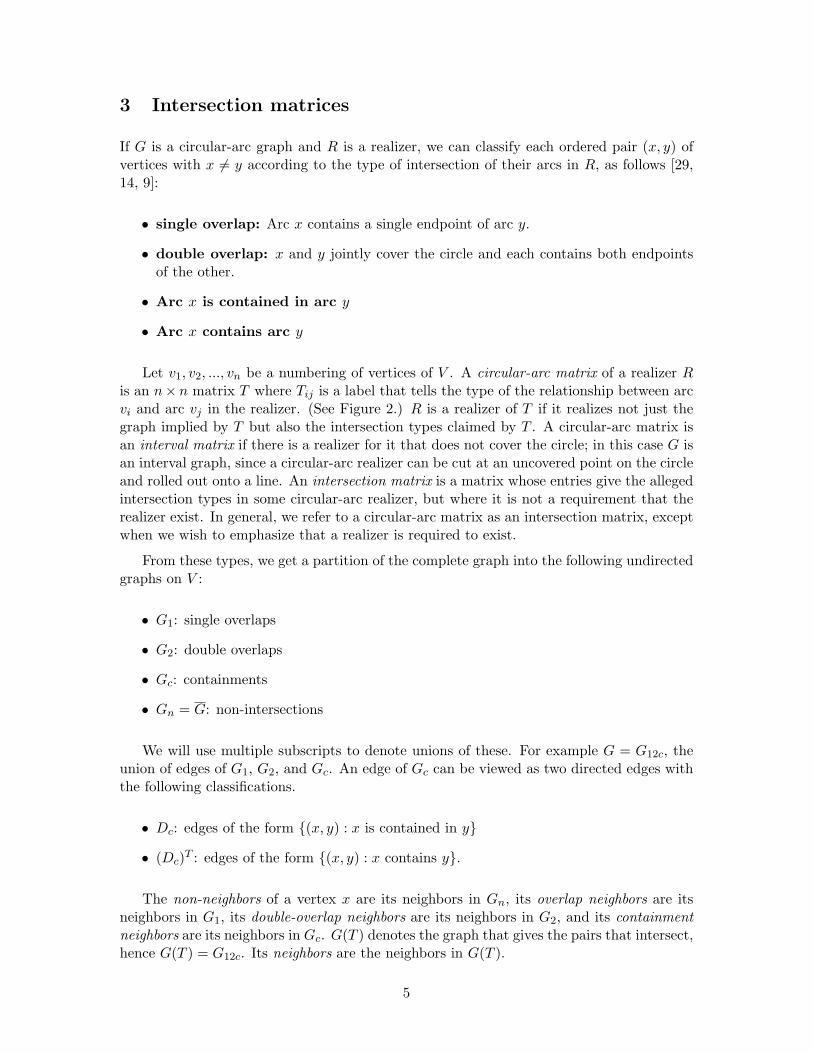
A departure of our approach from previous ones is the use of a simple operation onthe intersection matrix, which we will call a flip. Recall that we consider a realizer to bea circular list giving the order of left and right endpoints of the vertices’ arcs around thecircle. Let a geometric flip on a vertex be an exchange of the positions of l(x) and r(x) inthis list. This is equivalent to making x’s arc travel between the same endpoints as before,but around the opposite part of the circle as before (Figure 3). This changes the types ofrelationships involving x’s arc as follows:

• (x, y) ∈ G2 becomes (x, y) ∈ Dc and (x, y) ∈ Dc becomes (x, y) ∈ G2

• (x, y) ∈ Gn becomes (x, y) ∈ (Dc)T and (x, y) ∈ (Dc)T becomes (x, y) ∈ Gn

• (x, y) ∈ G1 remains unchanged

If T is an intersection matrix, we can compute the intersection matrix T ′ for the realizerthat results from a flip on x without any knowledge about the realizer, other than what isgiven directly by T . It requires only a simple relabeling of some of the entries of x’s rowand column in T . Let us call this relabeling of T an algebraic flip on x.

One matrix being obtainable from another by a sequence of algebraic flips is an equiv-alence relation on intersection matrices. Let us call this relation flip-equivalence. Everyflip-equivalence class on circular-arc matrices contains an interval matrix: in a circular-arcrealizer of a matrix T , if one picks a point on the circle that does not coincide with anendpoint of an arc and flips all arcs containing the point, the resulting set of arcs will failto cover the circle at that point, and realize the interval matrix T ′ obtained from T by theequivalent algebraic flips.

6

ef

dc

b a

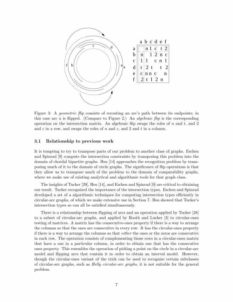
a n 1 c t 2b n 1 2 n cc 1 1 c n 1d t 2 t t 2e c n n c nf 2 t 1 2 n

a b c d e f

Figure 3: A geometric flip consists of rerouting an arc’s path between its endpoints; inthis case arc a is flipped. (Compare to Figure 2.) An algebraic flip is the correspondingoperation on the intersection matrix. An algebraic flip swaps the roles of n and t, and 2and c in a row, and swaps the roles of n and c, and 2 and t in a column.

3.1 Relationship to previous work

It is tempting to try to transpose parts of our problem to another class of graphs. Eschenand Spinrad [9] compute the intersection constraints by transposing this problem into thedomain of chordal bipartite graphs. Hsu [14] approaches the recognition problem by trans-posing much of it to the domain of circle graphs. The significance of flip operations is thatthey allow us to transpose much of the problem to the domain of comparability graphs,where we make use of existing analytical and algorithmic tools for that graph class.

The insights of Tucker [29], Hsu [14], and Eschen and Spinrad [9] are critical to obtainingour result. Tucker recognized the importance of the intersection types. Eschen and Spinraddeveloped a set of a algorithmic techniques for computing intersection types efficiently incircular-arc graphs, of which we make extensive use in Section 7. Hsu showed that Tucker’sintersection types so can all be satisfied simultaneously.

There is a relationship between flipping of arcs and an operation applied by Tucker [28]to a subset of circular-arc graphs, and applied by Booth and Lueker [3] to circular-onestesting of matrices. A matrix has the consecutive-ones property if there is a way to arrangethe columns so that the ones are consecutive in every row. It has the circular-ones propertyif there is a way to arrange the columns so that either the ones or the zeros are consecutivein each row. The operation consists of complementing those rows in a circular-ones matrixthat have a one in a particular column, in order to obtain one that has the consecutiveones property. This resembles the operation of picking a point on the circle in a circular-arcmodel and flipping arcs that contain it in order to obtain an interval model. However,though the circular-ones variant of the trick can be used to recognize certain subclassesof circular-arc graphs, such as Helly circular-arc graphs, it is not suitable for the generalproblem.

7

4 Summary of the circular-arc graph recognition algorithm

In Section 5, we show that it is possible to check in time linear in the size of a graph G plusthe size of a circular-arc realizer R whether G is the graph realized by R. Our approachto recognizing circular-arc graphs is then to give an algorithm that has, as a precondition,that its input be a circular-arc graph G, and that produces a circular-arc realizer of G inlinear time whenever the precondition is met. As long as this algorithm halts when itsprecondition is not met, it suffices to recognize circular-arc graphs: we may check whetherits output, if it produces any, is a circular-arc realizer of G. Since no circular-arc realizercan realize G if G is not a circular-arc graph, the test succeeds iff G is a circular-arc graph.

Let us now consider the time bound. If G is a circular-arc graph, our recognitionalgorithm runs in linear time. That is, there exists some constant c such that the algorithmhalts before c(n + m) operations have been executed. Therefore, there exists an algorithmthat runs our algorithm and halts, rejecting G, if the number of operations executed exceedsc(n+m). This proves that circular-arc graphs can be recognized in linear time. This resultis the primary goal of the paper.

It is worth noting that a programmer who wishes to implement the algorithm wouldwish to have conventional halting conditions that do not require counting operations or acareful analysis of the constant hidden in our big-O bound. However, for most steps, theanalysis of the time bound does not depend on whether the input graph is a circular-arcgraph. Other steps have a precondition that will be met if the input is a circular-arc graph,so that the input graph may be rejected early if the precondition is not met. Henceforth,we will assume throughout the analysis that G is a circular-arc graph, except where weaddress this issue.

Algorithm 4.1 summarizes the approach to producing a circular-arc realizer.

Algorithm 4.1 Constructing a circular-arc realizer.

1. Find an intersection matrix T that can be shown to be realized by some realizer of G;

2. Perform a set of algebraic flips on T to obtain an interval matrix T ′;

3. Find an interval realizer R′ of T ′;

4. Invert the flips used to obtain T ′ from T , but apply them as geometric flips to R′, toobtain a circular-arc realizer R of T .

The fourth subproblem is trivial. We summarize the approach to the other three now,and give the full details in later sections.

4.1 Step 1: Finding an intersection matrix that gives the intersectiontypes for some realizer of G

A universal vertex is a vertex x with N [x] = V . A module of an undirected graph is a setX of vertices such that for every vertex y 6∈ X, either y is a neighbor of every member ofX or it is a neighbor of none of them. A clique module is a module of G that is a (notnecessarily maximal) clique in G.

8

We use a reduction that allows us to assume that G has no universal vertex or cliquemodule. The following then gives the basic recipe for producing the desired intersectionmatrix.

Definition 4.2 Let T (G) denote the n× n matrix T of labels that is defined as follows:

1. if x and y are nonadjacent then Txy = n

2. else if N [x] ⊂ N [y] then Txy = c

3. else if N [y] ⊂ N [x] then Txy = t

4. else if N [x] ∪ N [y] = V and for each z ∈ N [x] − N [y], N [z] ⊂ N [x] and for eachz′ ∈ N [y]−N [x], N [z′] ⊂ N [y], then Txy = 2

5. else Txy = 1

Hsu has shown that if G is a circular-arc graph without universal vertices or cliquemodules, any realizer of the intersection matrix T (G) given by Definition 4.2 is a realizerof G [14]. It is not hard to see why this might be the case. If N [x] ⊂ N [y], then in arealizer where arc x is not contained in arc y, one endpoint of x may be shortened to makeit be contained in y without causing x to lose any neighbors. If x and y have a doubleoverlap, then they jointly cover the circle, hence N [x] ∪ N [y] = V . However, even whenN [x] ∪N [y] = V , x and y cannot have a double overlap if there exist z ∈ N [x]−N [y] andz′ ∈ N [y] − N [x] that are adjacent to each other. The x and y must fail to contain theintersection of arcs z and z′, hence they cannot jointly cover the whole circle. The subtlepoint of Hsu’s result is showing that there is a single realizer of G that simultaneously obeysall of these constraints.

This reduces the step to the problem of evaluating the boolean expressions of parts 2,3, and 4 of Definition 4.2 at each edge xy of G.

We use a sparse representation of the matrix where we label the edges of G with theirintersection types, which must fall into cases 2-5. This saves us from having to spendtime on entries of the matrix corresponding to Case 1. When we flip a vertex a, we musttherefore add, delete, and relabel edges from this graph. This requires keeping a pointerfrom each adjacency-list entry (a, b) to its twin (b, a), and implementing the adjacency listswith doubly-linked lists.

Eschen and Spinrad have given O(n2) bounds for evaluating N [x] ⊂ N [y], N [y] ⊂ N [x],and N [x] ∪N [y] = V at all pairs x, y of vertices. We show how to apply their techniquein O(n + m) time if one needs to evaluate it only at the m adjacent pairs of G.

This allows us to produce T (G), except that it does not allow us to distinguish betweencases 4 and 5 if N [x] ∪N [y] = V . That is, it does not allow us to tell in this case whethertwo adjacent arcs have a single overlap or a double overlap. The key insight for solvingthis problem is that if x and y have a double overlap, then flipping y causes y’s interval tobe contained in x’s, hence it causes N [y] to become a subset of N [x]. Flipping y reducesthe problem to the foregoing one of testing whether a neighborhood containment appliesbetween a pair of adjacent vertices, but on a modified graph where x is flipped.

The details of this step are given in Section 7.

9

4.2 Step 2: Finding a set of flips to turn T into an interval matrix

The goal of this step is to identify the set of vertices whose arcs contain a point on thecircle in a realizer of the intersection matrix. Flipping them vacates this part of the circle,giving an interval matrix.

What makes the step difficult is that, unlike in the case of an interval graph, the verticesof a clique do not have to have a common intersection point. For instance, the arcs [0, π],[2π/3, 5π/3], and [3π/2, π/2] form a clique but have no common intersection point on thecircle. Therefore, it does not suffice to identify a maximal clique.

However, suppose that a vertex v0 has no incident edges in Gd and Gc. Then everyneighbor of the vertex in G is a neighbor in G1. In a realizer, every neighbor contains oneand only one endpoint of this vertex’s arc. Those that contain one endpoint have a commonintersection and those that contain the other have a common intersection. We then needonly to identify the neighbors that contain one of the endpoints.

Such a v0 might not exist initially, but it is easy to obtain one with some initial flips inorder to isolate it in Gd and Gc. The one that we create has degree O(m/n). This allows usto spend O(n) time on each neighbor of the vertex without violating the linear time bound.This is adequate to be able to perform an arbitrary set of flips on neighbors of v0.

To identify which neighbors of v0 cover one endpoint, we use a combination of constraintsimposed by their relationships to each other and by their relationships to the non-neighbors.For instance, two neighbors that have a Gd or Gn relationship to each other must coveropposite endpoints. Let W be the non-neighbors. Suppose x and y are neighbors of v0

that have properly overlapping sets of neighbors in W . That is, N [x] ∩W and N [y] ∩Wintersect but neither of these sets contains the other. Then x and y must obviously coveropposite endpoints of v0 in a circular-arc realizer.

In practice, our approach is to begin to partition neighbors of v0 according which end-point of v0 they cover. Partway through this process, we observe that the set of arcs thatcontain a third point on the circle is easy to identify. This allows us to quit early, since thisset of arcs is also a solution to the problem.

The details of this step are given in Section 8.

4.3 Step 3: Finding an interval realizer of an interval matrix

It is easily seen that if T is an interval matrix, Gn is a comparability graph: the order ofleft endpoints in an interval realizer is a linear extension of a transitive orientation. (SeeFigure 4.) G1n is a comparability graph for the same reason. In an interval matrix, G2

is empty, since a double overlap of two arcs covers the entire circle. Therefore, Gc is thecomplement of G1n. Since it also has a transitive orientation, namely Dc, it follows thatGc and G1n are complementary comparability graphs, hence permutation graphs.

In [18], an algorithm is given for interval-graph recognition that uses a linear extensionof a transitive orientation of G = Gn. Thus, we can get an interval realizer of G in thisway. Unfortunately, because of the added constraints in the types of intersections imposedby T , this might fail to be a realizer of T .

The permutation-graph recognition algorithm of [18] uses the transitive orientation al-

10

gorithm to compute linear extensions of transitive orientations D and D′ of a permutationgraph H and its complement H. It then finds the linear orders D ∪D′ and D ∪ (D′)T inlinear time, which gives the permutation realizer. Running this algorithm gives a linearextension of Dc and a linear extension of a transitive orientation G1n, and therefore gives apermutation realizer of G1n. It is easy to see that these two permutations are the order ofappearance of left endpoints and the order of appearance of right endpoints in an intervalrealizer of G. But once again, this may fail to be an interval realizer of T .

The key observation we use is that every realizer of T gives a single orientation ofG1n that is simultaneously transitive in G1n and Gn. Finding a transitive orientation ofG1n that is simultaneously transitive in Gn further constrains the possible solutions, andallows us to get the orders of appearance of left and of right endpoints of a realizer of T .Interleaving these orders to produce the full realizer is a trivial operation. We show howthe transitive orientation algorithm of [18] can be modified to produce the simultaneoustransitive orientations of G1n and Gn.

The details of this step are given in Section 7.

5 Verifying a proposed realizer

The correctness of our analysis depends on the claim, made earlier, that it is possible toverify in time linear in the size of G plus the size of a realizer R that R realizes G. Weassume that R is presented as a list of arc endpoints and the vertices to which they belong,in the order in which they occur counter-clockwise about the circle. When G is a circular-arcgraph, our algorithm produces the realizer in this format.

Algorithm 5.1 Checking whether a circular-arc realizer realizes G.

Pick a starting point on the circle and make a doubly-linked list L of all arcs that containthat point, in O(n) time. Then travel counter-clockwise, updating L whenever an endpointof some arc x is encountered, so that it reflects the set of arcs that contain the current point.This requires adding x to L in O(1) time if the encountered endpoint is a left endpoint, andremoving it in O(1) time (L is doubly-linked) if the encountered endpoint is a right endpoint.Regardless of whether the endpoint is a left or right endpoint, generate the following edgerecords: (y, x) : y ∈ L and (x, y) : y ∈ L. Halt when either the starting point on thecircle has been reached again, or the total number of generated edge records exceeds 8m.Reject the realizer if the number of generated edge records exceeds 8m. Otherwise, radixsort the generated edge records and throw out duplicates. Then concatenate the adjacencylists of G and radix sort them. Verify that these two operations produce identical lists.

For the correctness and time bound, note that if x and y are adjacent, each contains atmost two endpoints of the other. Therefore, if the realizer is valid, at most four copies of(x, y) will be generated, and at most four copies of (y, x) will be generated. The realizercan be rejected if the number of generated edge records exceeds 8m. The radix sorts takesO(n + m) time, and comparing the lists establishes whether G is identical to the graphrepresented by the realizer. The algorithm takes O(n) time for all updates of L, and O(1)time for each generated edge record, for a total of O(n + m).

11

6 Details of Step 3: Finding an interval realizer of an intervalmatrix

Even though this section deals with the third step of Algorithm 4.1, we give it before thesections on the first two steps. It is of greatest interest to most readers, and develops aresult that is used in a less obvious way in Step 2. (However, Subsection 6.4.5 is of interestprimarily to specialists, and can be skipped without loss of continuity.)

Recall that an interval matrix is the intersection matrix of an interval realizer. In thissection, we deal with the problem of finding an interval realizer of an interval matrix. Sinceintervals on a line cannot realize a double-overlap relation, we may assume that the matrixis devoid of entries labeled 2 for the G2 relation.

6.1 Basic Tools

An undirected graph is a special case of a directed graph where each undirected edgeconsists of two oppositely directed edges. In this paper, we consider an n × n matrix Ato be synonymous with a complete graph on vertex set V = v1, v2, ..., vn, where eachdirected edge (vi, vj) is labeled with Aij .

A module of a matrix corresponds to a set X of vertices such that for every vertexy 6∈ X, all directed edges in X ×y have the same label, and all directed edges in y×Xhave the same label. In this case, y fails to distinguish members of X. A module of a graphor digraph G = (V,E) is a module in its boolean adjacency matrix. That is, it is a set ofvertices such that for each y 6∈ X, every element of X×y is an edge or none is, and everyelement of y ×X is an edge or none is. Modules of matrices are studied in [6, 7]. Theywere previously known in the special case of graphs, and first studied in [11].

The set V and its singleton subsets are trivial modules. A graph or matrix with onlytrivial modules is called prime.

A modular partition of V in a matrix is a partition of V where every partition class isa module. If X and Y are disjoint modules, then every element of X × Y has the samelabel. The modular quotient induced by the parts is the matrix obtained by making onevertex for each part, and letting the label of each ordered pair (X, Y ) of parts be the labelsof the edges from X to Y . One way to represent a modular quotient is with the submatrixinduced by any set P consisting of one vertex from each part. Similarly, if R is a circular-arcrealizer, then the quotient is realized with the smaller realizer R|P .

Two sets A and B overlap if A ∩B, A−B, and B − A are all nonempty. A module isstrong if it overlaps no other module. The transitive reduction of the containment relationon strong modules of a graph G = (V,E) is a tree, and is called the modular decomposition.The root of the modular decomposition is V and the leaves are its singleton subsets. If G isundirected, at most one of G and its complement, G, can be disconnected. If one of them isdisconnected, the children of the root are the connected components, and V is a degeneratenode. The remaining nodes are prime nodes. The family F of modules of G consists ofthose sets that are nodes of the tree, and those sets that are a union of siblings that have adegenerate parent. Let MD(G) denote the modular decomposition of an undirected graphG.

12

The modular decomposition of a symmetric matrix is defined in the same way, exceptthat the root is degenerate if the complement of the graph consisting of those edges withone label is disconnected. Let MD(T ) denote its modular decomposition of a symmetricmatrix T .

An undirected graph can be viewed as a special case of a directed graph, where eachundirected edge ab represents two directed edges, (a, b) and (b, a). If (a, b) and (c, d) aretwo directed edges, we say that (a, b)Γ(c, d) iff a = c and b and d are nonadjacent, or b = dand a and c are nonadjacent. If G is a comparability graph, then (a, b)Γ(c, d) implies thatin any transitive orientation of G, either both of (a, b) and (c, d) appear as directed edges,or neither does. To understand why, suppose that (a, b)Γ(c, d), but (a, b) and (d, c) aredirected edges in an orientation of G. Suppose without loss of generality that a = c. Then(d, c) and (c, b) require a transitive directed edge (d, b), but d and b are nonadjacent, so thisis impossible.

The transitive closure of the Γ relation is an equivalence relation on directed edges, andthe equivalence classes are groups of directed edges, called implication classes, that musteither all appear in or all be absent from any transitive orientation of G. Therefore, if G is acomparability graph, (a, b) and its transpose (b, a) cannot be in the same implication class.The implication class containing (a, b) consists of the transposes of the directed edges inthe implication class containing (b, a). The union of an implication class and its transposeis a color class. The color classes are a partition of the undirected edges of G.

There is a type of dual relationship between the modules of G and its color classes.

Lemma 6.1 (see, for example, [22]) If X and Y are disjoint nodes of the modular decom-position of G, then X × Y is a subset of a single implication class.

The vertices spanned by a color class are always a module of G. Moreover, if M isa module, an edge of G that is in G|M is always in a different color class from an edgethat is not in G|M . Because of this, given a transitive orientation of G and its modulardecomposition, one may obtain a new transitive orientation by reversing the directions ofall edges inside a node of the modular decomposition tree. In a degenerate node whosechildren are nonadjacent in G, a transitive orientation of G determines a linear order onthe children. Reversing the orientations of all edges between a pair of children that areadjacent in this linear order gives a new transitive orientation. All transitive orientationsof G are obtainable from a single one by applying these two reversal operations in differentplaces in the modular decomposition tree.

It is not the case that every interval realizer of an interval graph G realizes the in-tersection matrix given by a particular realizer R of G. This is because its partition ofedges of G into Dc, G1, and G2 relations given by a different realizer R′ of G may not befaithfully reflected by the types of intersections in R’s matrix. Therefore, an intersectionmatrix places additional constraints on possible realizers that G does not place, and not allrealizers of G satisfy the requirements of Step 3.

6.2 Interval Orientations

Let T be an interval matrix and R be an interval realizer of T . If ab ∈ G1n, let us say thata precedes b in R if l(a) < l(b), even if they overlap at one endpoint. (Because ab ∈ G1n,

13

a

b c

d e

f g

Orientation of Ginduced by R

a

b c

d e

f g

Orientation of Ginduced by R

1n

a

b c

d e

f g

a

b c d gf

e

n D (containments in R)c

Interval realizer R

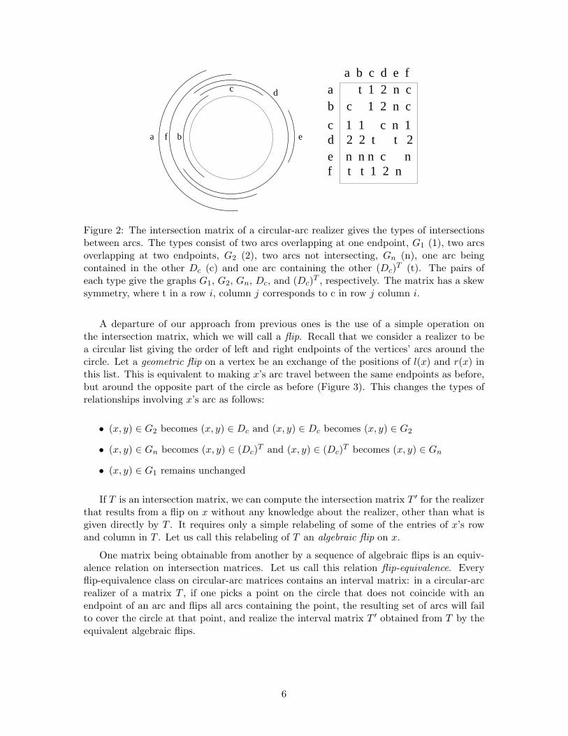
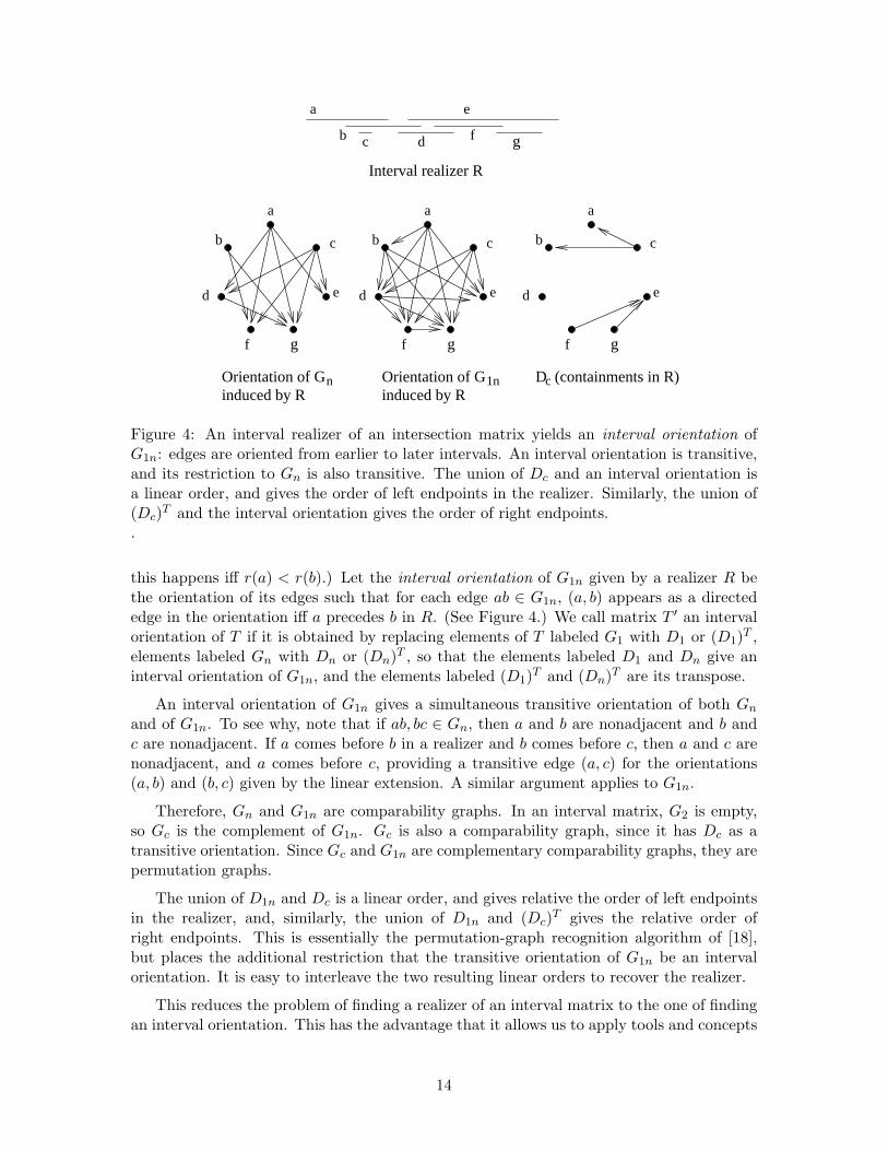
Figure 4: An interval realizer of an intersection matrix yields an interval orientation ofG1n: edges are oriented from earlier to later intervals. An interval orientation is transitive,and its restriction to Gn is also transitive. The union of Dc and an interval orientation isa linear order, and gives the order of left endpoints in the realizer. Similarly, the union of(Dc)T and the interval orientation gives the order of right endpoints..

this happens iff r(a) < r(b).) Let the interval orientation of G1n given by a realizer R bethe orientation of its edges such that for each edge ab ∈ G1n, (a, b) appears as a directededge in the orientation iff a precedes b in R. (See Figure 4.) We call matrix T ′ an intervalorientation of T if it is obtained by replacing elements of T labeled G1 with D1 or (D1)T ,elements labeled Gn with Dn or (Dn)T , so that the elements labeled D1 and Dn give aninterval orientation of G1n, and the elements labeled (D1)T and (Dn)T are its transpose.

An interval orientation of G1n gives a simultaneous transitive orientation of both Gn

and of G1n. To see why, note that if ab, bc ∈ Gn, then a and b are nonadjacent and b andc are nonadjacent. If a comes before b in a realizer and b comes before c, then a and c arenonadjacent, and a comes before c, providing a transitive edge (a, c) for the orientations(a, b) and (b, c) given by the linear extension. A similar argument applies to G1n.

Therefore, Gn and G1n are comparability graphs. In an interval matrix, G2 is empty,so Gc is the complement of G1n. Gc is also a comparability graph, since it has Dc as atransitive orientation. Since Gc and G1n are complementary comparability graphs, they arepermutation graphs.

The union of D1n and Dc is a linear order, and gives relative the order of left endpointsin the realizer, and, similarly, the union of D1n and (Dc)T gives the relative order ofright endpoints. This is essentially the permutation-graph recognition algorithm of [18],but places the additional restriction that the transitive orientation of G1n be an intervalorientation. It is easy to interleave the two resulting linear orders to recover the realizer.

This reduces the problem of finding a realizer of an interval matrix to the one of findingan interval orientation. This has the advantage that it allows us to apply tools and concepts

14

c

d

b

a

w

z

x

c

d

b

a

xw

z y

ab

dc

w

z

x

A B

C D E

G

xw

z y

ab

dc

w

z

x

c

d

b

a

G

G’

G’

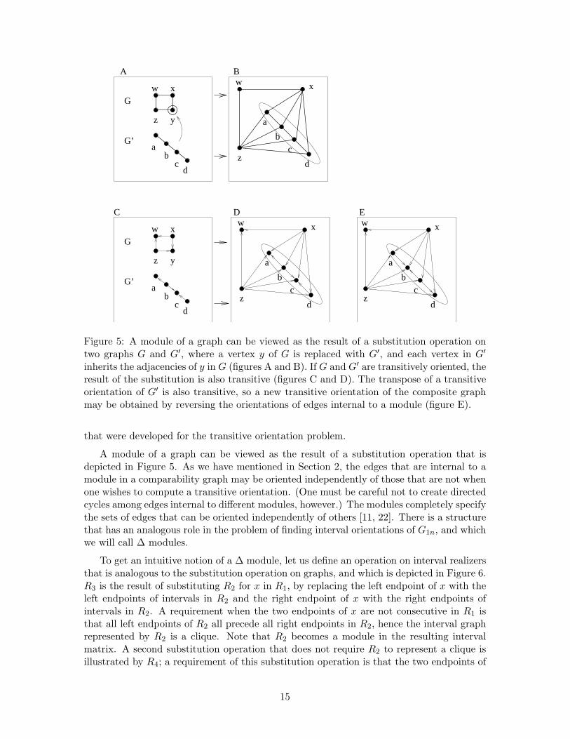
Figure 5: A module of a graph can be viewed as the result of a substitution operation ontwo graphs G and G′, where a vertex y of G is replaced with G′, and each vertex in G′

inherits the adjacencies of y in G (figures A and B). If G and G′ are transitively oriented, theresult of the substitution is also transitive (figures C and D). The transpose of a transitiveorientation of G′ is also transitive, so a new transitive orientation of the composite graphmay be obtained by reversing the orientations of edges internal to a module (figure E).

that were developed for the transitive orientation problem.

A module of a graph can be viewed as the result of a substitution operation that isdepicted in Figure 5. As we have mentioned in Section 2, the edges that are internal to amodule in a comparability graph may be oriented independently of those that are not whenone wishes to compute a transitive orientation. (One must be careful not to create directedcycles among edges internal to different modules, however.) The modules completely specifythe sets of edges that can be oriented independently of others [11, 22]. There is a structurethat has an analogous role in the problem of finding interval orientations of G1n, and whichwe will call ∆ modules.

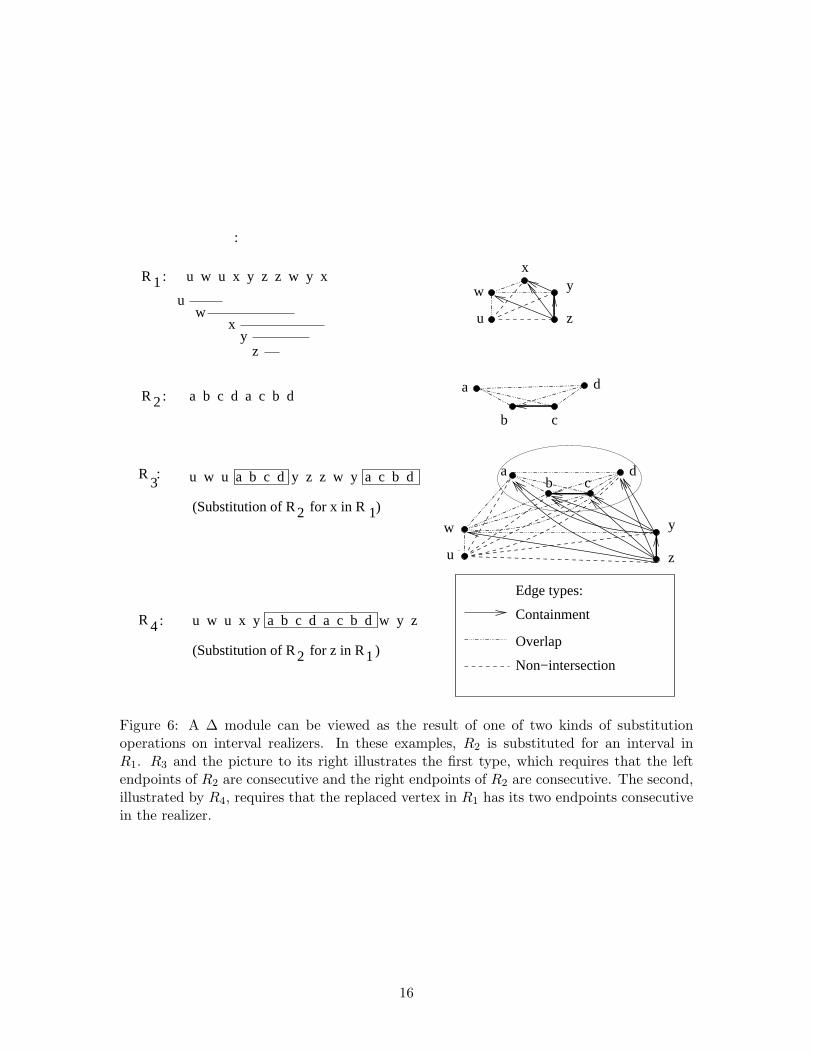
To get an intuitive notion of a ∆ module, let us define an operation on interval realizersthat is analogous to the substitution operation on graphs, and which is depicted in Figure 6.R3 is the result of substituting R2 for x in R1, by replacing the left endpoint of x with theleft endpoints of intervals in R2 and the right endpoint of x with the right endpoints ofintervals in R2. A requirement when the two endpoints of x are not consecutive in R1 isthat all left endpoints of R2 all precede all right endpoints in R2, hence the interval graphrepresented by R2 is a clique. Note that R2 becomes a module in the resulting intervalmatrix. A second substitution operation that does not require R2 to represent a clique isillustrated by R4; a requirement of this substitution operation is that the two endpoints of

15

u w u a b c d y z z w y a c b dR3

u w u x y a b c d a c b d w y zR 4

y

z

y

z

(Substitution of R for x in R )2 1

(Substitution of R for z in R )2 1

u w u x y z z w y x

a b c d a c b d

uw

xy

z

R

R

2

1

Non−intersection

Overlap

Containment

:

:

:

:

:

Edge types:

u

w

x

b c

da

u

w

ab c

d

Figure 6: A ∆ module can be viewed as the result of one of two kinds of substitutionoperations on interval realizers. In these examples, R2 is substituted for an interval inR1. R3 and the picture to its right illustrates the first type, which requires that the leftendpoints of R2 are consecutive and the right endpoints of R2 are consecutive. The second,illustrated by R4, requires that the replaced vertex in R1 has its two endpoints consecutivein the realizer.

16

c

a b

G0

G (proper overlap)1

(non−intersection)

c

b a

a b

c

c

a b

c

a b

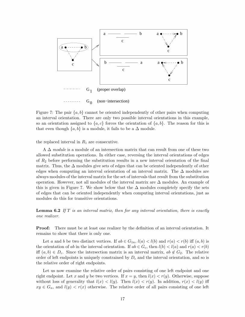
Figure 7: The pair a, b cannot be oriented independently of other pairs when computingan interval orientation. There are only two possible interval orientations in this example,so an orientation assigned to a, c forces the orientation of a, b. The reason for this isthat even though a, b is a module, it fails to be a ∆ module.

the replaced interval in R1 are consecutive.

A ∆ module is a module of an intersection matrix that can result from one of these twoallowed substitution operations. In either case, reversing the interval orientations of edgesof R2 before performing the substitution results in a new interval orientation of the finalmatrix. Thus, the ∆ modules give sets of edges that can be oriented independently of otheredges when computing an interval orientation of an interval matrix. The ∆ modules arealways modules of the interval matrix for the set of intervals that result from the substitutionoperation. However, not all modules of the interval matrix are ∆ modules. An example ofthis is given in Figure 7. We show below that the ∆ modules completely specify the setsof edges that can be oriented independently when computing interval orientations, just asmodules do this for transitive orientations.

Lemma 6.2 If T is an interval matrix, then for any interval orientation, there is exactlyone realizer.

Proof: There must be at least one realizer by the definition of an interval orientation. Itremains to show that there is only one.

Let a and b be two distinct vertices. If ab ∈ G1n, l(a) < l(b) and r(a) < r(b) iff (a, b) isthe orientation of ab in the interval orientation. If ab ∈ Gc, then l(b) < l(a) and r(a) < r(b)iff (a, b) ∈ Dc. Since the intersection matrix is an interval matrix, ab 6∈ G2. The relativeorder of left endpoints is uniquely constrained by Dc and the interval orientation, and so isthe relative order of right endpoints.

Let us now examine the relative order of pairs consisting of one left endpoint and oneright endpoint. Let x and y be two vertices. If x = y, then l(x) < r(y). Otherwise, supposewithout loss of generality that l(x) < l(y). Then l(x) < r(y). In addition, r(x) < l(y) iffxy ∈ Gn, and l(y) < r(x) otherwise. The relative order of all pairs consisting of one left

17

endpoint and one right endpoint are uniquely constrained. 2

6.3 A Γ-like relation for interval orientations

Let us define an analog ∆ of the Γ relation for the problem of finding an interval orientationinstead of just a transitive orientation. (The Γ relation involves two edges joined at oneend, resembling the letter Γ, while ∆ involves three relationships that make a triangle.) LetΓn denote the Γ relation on Gn, let Γ1 denote the Γ relation on G1, and let Γ1n denote theΓ relation on G1n.

Definition 6.3 Let a, b, c be three vertices. Then (a, b)∆(a, c) and (b, a)∆(c, a) if one ofthe following applies:

• (a, b)Γn(a, c) (i.e. ab, ac ∈ Gn and bc ∈ G1c);

• (a, b)Γ1n(a, c) (i.e. ab, ac ∈ G1n and bc ∈ Gc);

• ab ∈ Gn and bc, ac ∈ G1.

Let us call the last of the conditions in the definition of ∆ a straddle relationship, sincethe edges ac, bc ∈ G1 “straddle” edge ab ∈ Gn.

By analogy to Γ, we let the ∆ implication classes be the equivalence classes of thetransitive symmetric closure of ∆, and the ∆ color classes be the union of each equivalenceclass and its transpose.

Theorem 6.4 Every interval orientation of G1n in an interval matrix consists of one ∆implication class from each ∆ color class.

Proof: For every edge ab ∈ G1n, exactly one of (a, b) or (b, a) appears in any intervalorientation. An interval orientation is a transitive orientation of Gn, so if (a, b)Γn(a, c) thenboth or neither appear in any transitive orientation of Γn. It is also a transitive orientationof G1n, so if (a, b)Γ1n(a, c) then both or neither appear in any transitive orientation of Γ1n.If (a, b)∆(a, c) by the straddle condition, with ab ∈ Gn and ac, bc ∈ G1, then a and b containopposite endpoints of c in any interval realizer. The order of left endpoints must be (a, c, b)or (b, c, a). Either both or neither of (a, b) and (a, c) appear in any interval orientation. 2

We now show that ∆ has the same dual relationship with the ∆ modules as Γ has withmodules of a graph. Every ∆ module is a module, but some modules are not ∆ modules.Like the set of modules, the ∆ modules have a decomposition tree where every node isprime or degenerate, and where a set is a member of the family iff it is a node of the treeor a union of children of a degenerate node. The tree is not the modular decompositiontree, however. Just as in the case of Γ, the spans of the equivalence classes induced by ∆are nodes of the tree and pairs of children of degenerate nodes.

Definition 6.5 Let T be an interval matrix. Let U(T ) denote the matrix obtained fromT by replacing each instance of Dc or (Dc)T with Gc, thereby “unorienting” the directededges in Dc. (We define U(T ) so that we may avoid dealing with details of the modular

18

decomposition of a matrix that is not symmetric.) Let us say that a set M of verticesoverlaps a set E′ of edges of T if T |M contains some members, but not all members, of E′.A module of T or of U(T ) is a ∆ module if it is a module that is a clique of G(T ), or elsea module X such that for no y ∈ V −X, y ×X ⊆ G1.

It is well-known that no module of a graph overlaps a Γ color color class [12]. Thefollowing is an analogous result about ∆ modules and ∆ color classes:

Lemma 6.6 No ∆ module overlaps a ∆ color class.

Proof: A module M of U(T ) is a module of Gn and a module of G1n. Therefore, itcannot overlap a pair of edges that are related by the first two conditions of the definitionof ∆. For the third condition, M must be a module of G1. If it contains a, c, it mustcontain b, c, which implies that it contains a, b. If it contains a, b, then it is not aclique. If c ∈ V −M , then c ×M ⊆ G1, and it is not a ∆ module of U(T ). 2

Definition 6.7 A family F of subsets of a set V is a tree-decomposable family if it satisfiesthe following properties:

1. V and the members of x : x ∈ V are members of F .

2. Overlap closure: If X and Y are properly overlapping members of F , then X ∪ Y ,X ∩ Y , X − Y , Y −X, and (X − Y ) ∪ (Y −X) are members of F .

The strong members of F are those members that properly overlap with no other memberof F .

Theorem 6.8 [23, 24, 6, 7] If F is a tree-decomposable family, then the transitive reductionof the containment relation on strong members of F is a tree. There is a unique way tolabel the nodes of this tree prime and degenerate so that a set is a member of F iff it is anode of the tree or a union of children of a degenerate node.

Let us call this tree the tree decomposition of F . The modular decomposition of anundirected graph or a symmetric matrix is just the tree decomposition of its modules,which are a tree-decomposable family.

Theorem 6.9 The ∆ modules of U(T ) are a tree-decomposable family.

Proof: The modules of a symmetric matrix are a tree-decomposable family [6, 7]. Let Xand Y be overlapping ∆ modules. Since they are modules, X ∪ Y , X ∩ Y , X − Y , Y −X,and (X −Y )∪ (Y −X) are modules. If X and Y are both cliques of G(T ), then vertices inX − Y have edges in G(T ) to X ∩ Y , hence to all of Y . X ∪ Y is a clique, so all modulesthat are subsets of X ∪ Y are ∆ modules, and the claim holds.

Let us therefore assume in the remainder of the proof that X is not a clique.

19

We now show that X ∩Y is a ∆ module. If X ∩Y is a clique, then, since it is a module,it is a ∆ module. Otherwise, neither X nor Y is a clique. Since both of these sets are∆ modules, there exists no G1 edges from members of X to vertices outside of X, or G1

edges from members of Y to vertices outside of Y . An edge from a vertex of X ∩ Y to avertex outside of X ∩ Y either goes from a member of X to a non-member of X, or froma member of Y to a non-member of Y . Therefore, there is no edge of G1 from X ∩ Y to avertex outside X ∩ Y . Since X ∩ Y is a module, it must be a ∆ module.

Next, we show that X − Y is a ∆ module. If X − Y is a clique, it is a ∆ module, sinceit is a module. If X − Y is not a clique, then since X is a ∆ module, any w ∈ V − (X − Y )such that w × (X − Y ) ⊆ G1 must reside in X ∩ Y . Suppose such a w exists. Since wresides in Y and Y is a module, (X − Y ) × Y ⊆ G1. For w′ ∈ Y −X, w′ ×X ⊆ G1, acontradiction, since X is a ∆ module. The same analysis applies to Y −X.

Finally, we show that U = (X − Y ) ∪ (Y −X) is a ∆ module. If U is a clique, it a ∆module, since it is a module. Otherwise, any vertex w ∈ V − U such that w × U ⊆ G1

must lie inside X, since X is a ∆ module and not a clique. Therefore, w ∈ X ∩Y . Since Xis a module and (Y −X)×w ⊆ G1, (Y −X)×X ⊆ G1. (X −Y )∪ (Y −X) can only failto be a clique if X − Y or Y −X fails to be a clique. Suppose X − Y fails to be a clique.Then X fails to be a clique. (Y −X)×X ⊆ G1 contradicts the assumption that X is a ∆module. 2

Definition 6.10 Let us call the tree decomposition of U(T ) the Delta tree of U(T ), anddenote it ∆(U(T )).

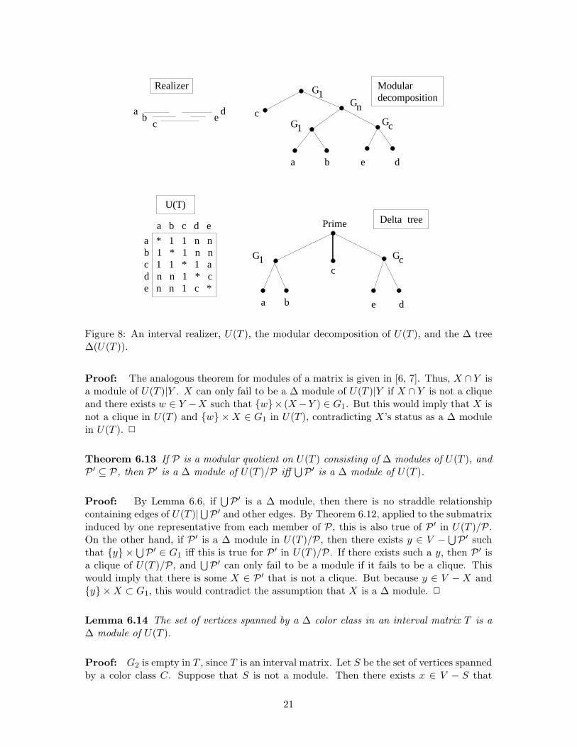
Just like the modular decomposition, ∆(U(T )) tree be represented in O(n) space bycreating a node of size O(1) to represent each node of ∆(U(T )), and giving each node alabel to indicate whether it is prime or degenerate as well as a list of pointers to its childrenin the transitive reduction of the containment relation. The quotient induced by childrenof a degenerate node in their parent is complete in Gn, G1, or Gc, so each degenerate nodemay be labeled according to which of these cases applies. The set U represented by a nodecan be retrieved in O(|U |) time by visiting its leaf descendants, so there is no advantage tolabeling a node with a list of its members. Figure 8 gives an example.

The following Theorems 6.11, 6.12, and 6.13 show that ∆ modules satisfy the remainingproperties of a class of set system described by Mohring in [23, 24].

Theorem 6.11 If X is a ∆ module of U(T ) and Y is a subset of X, then Y is a ∆ moduleof U(T ) iff it is a ∆ module of U(T )|X.

Proof: If Y is a clique, the claim holds because of the corresponding theorem aboutmodules of a matrix [6, 7]. If Y is not a clique, then neither is X, and since X is a ∆module, there exists no y ∈ V −X with an edge of G1 to any member of X, hence to anymember of y. Then Y fails to be a ∆ module in U(T ) iff there exists y ∈ X − Y with G1

edges to Y , which also determines whether it is a module of U(T )|X. 2

Theorem 6.12 If X is a ∆ module of U(T ) and Y ⊆ V intersects X, then X ∩ Y is a ∆module of U(T )|Y .

20

G1 Gc

Delta tree

Realizer

a dc

b e

a b c d e

a * 1 1 n nb 1 * 1 n nc 1 1 * 1 ad n n 1 * ce n n 1 c *

U(T)

G1

G1

Gn

Gc

Prime

a b

c

e d

e dba

c

Modulardecomposition

Figure 8: An interval realizer, U(T ), the modular decomposition of U(T ), and the ∆ tree∆(U(T )).

Proof: The analogous theorem for modules of a matrix is given in [6, 7]. Thus, X ∩ Y isa module of U(T )|Y . X can only fail to be a ∆ module of U(T )|Y if X ∩ Y is not a cliqueand there exists w ∈ Y −X such that w× (X−Y ) ∈ G1. But this would imply that X isnot a clique in U(T ) and w ×X ∈ G1 in U(T ), contradicting X’s status as a ∆ modulein U(T ). 2

Theorem 6.13 If P is a modular quotient on U(T ) consisting of ∆ modules of U(T ), andP ′ ⊆ P, then P ′ is a ∆ module of U(T )/P iff

⋃P ′ is a ∆ module of U(T ).

Proof: By Lemma 6.6, if⋃P ′ is a ∆ module, then there is no straddle relationship

containing edges of U(T )|⋃P ′ and other edges. By Theorem 6.12, applied to the submatrix

induced by one representative from each member of P, this is also true of P ′ in U(T )/P.On the other hand, if P ′ is a ∆ module in U(T )/P, then there exists y ∈ V −

⋃P ′ such

that y ×⋃P ′ ∈ G1 iff this is true for P ′ in U(T )/P. If there exists such a y, then P ′ is

a clique of U(T )/P, and⋃P ′ can only fail to be a module if it fails to be a clique. This

would imply that there is some X ∈ P ′ that is not a clique. But because y ∈ V −X andy ×X ⊂ G1, this would contradict the assumption that X is a ∆ module. 2

Lemma 6.14 The set of vertices spanned by a ∆ color class in an interval matrix T is a∆ module of U(T ).

Proof: G2 is empty in T , since T is an interval matrix. Let S be the set of vertices spannedby a color class C. Suppose that S is not a module. Then there exists x ∈ V − S that

21

has different relationships in T to members of S. C is connected, as only coincident edgesare related by ∆. Therefore, x has different relationships between two vertices y, z ∈ Ssuch that yz ∈ C. At least one edge from x to y, z is an edge of G1n; without loss ofgenerality, suppose that xy ∈ G1n. If xz ∈ Gc then (x, y)Γ1n(z, y), and xy ∈ C contradictingx’s non-membership in S.

Therefore, xy and xz are edges of G1n. Without loss of generality, suppose xy ∈ G1

and xz ∈ Gn. If yz ∈ Gn, then (x, z)Γn(y, z), and we again get the contradiction x ∈ S. Ifyz ∈ G1, then (y, z)∆(x, z) by the straddle rule, and again, we get the contradiction x ∈ S.Since x does not exist, we conclude that S is a module.

Suppose that S is a module that is not a ∆ module. Then it is not a clique, and thereexists w ∈ V − S such that w × S ⊆ G1. There exist s1, s2 ∈ S such that s1s2 ∈ Gn.

Suppose s1s2 ∈ C. Then (w, s1)∆(s2, s1), w is among the vertices spanned by C, hencew ∈ S, a contradiction. We conclude that C consists exclusively of edges of G1, ands1, s2 ∈ S such that s1s2 ∈ Gn and s1s2 is in a different color class C ′. Let P = (s1 =x1, x2, ..., xk = s2) be a simple path from s1 to s2 whose edges are drawn from C.

To obtain a contradiction with s2xi−1 ∈ G1, we show by induction that for each i from1 to k − 1, s2xi ∈ Gn and s2xi ∈ C ′. This is true for i = 1, since s2s1 ∈ G1 and s2s1 ∈ C ′.Suppose by induction that i > 1 and that it is true for i−1. Then xi−1xi ∈ G1, xi−1xi ∈ C,s2xi−1 ∈ Gn, and s2xi−1 ∈ C ′. If s2xi ∈ Gc or s2xi ∈ G1, then xi−1xi∆xi−1s2, contradictingC ′ 6= C. Thus, s2xi ∈ Gn, and (s2, xi)∆(s2, xi−1), hence s2xi, like s2xi−1, is an element ofC ′. 2

Theorem 6.15 A set of edges of G1n is a ∆ color class iff it is the set of edges of G1n

connecting children of a prime node in the ∆ tree of U(T ) or the set of edges of G1n

connecting a pair of children of a degenerate node. If X and Y are two children of a nodeof the tree, then no ∆ implication class contains both directed edges in X × Y and directededges in Y ×X.

Proof: Let uw be an edge of G1n. If uw connects two children of a prime node A, thenall ∆ modules that contains u and w contain A. The color class C containing uw mustspan A by Lemma 6.14. C cannot span a larger set or contain edges that are internal to achild of A, by Lemma 6.6, and the claim follows for C. If uw connects two children B1 andB2 of a degenerate node, an identical argument applies.

For the claim about the orientations of edges between X and Y , suppose first that Xand Y are two children of a degenerate node Z. If Z is a Gc node, the claim is vacuous.Otherwise, suppose that a, b ∈ X and c ∈ Y such that (a, c) and (c, b) are in one implicationclass. Let A and B be the partition of X such that A × c and c × B are in the sameimplication class. If Z is a Gn node, then by transitivity of orientations of Gn in intervalorientations, A× B ⊂ Gn, and B ∪ Y is a ∆ module of U(T ), contradicting X’s status asa strong ∆ module. If Z is a G1 node, then X and Y are cliques of G(T ). By transitivityof interval orientations of G1n, A × B ⊆ G1, and B ∪ Y is a ∆ module, which is again acontradiction. If Z is ∆ prime, that is, it has only trivial ∆ modules, then by Theorem 6.13,the submatrix induced by one representative vertex from each child of Z has only trivialmodules. The orientation of an edge of this substructure cannot be reversed in an intervalorientation without reversing all edges in it. If a is the representative of X and c is the

22

representative of Y , then replacing a with b gives an interval orientation of an isomorphicsubmatrix that differs only in the orientation of a single edge, a contradiction. 2

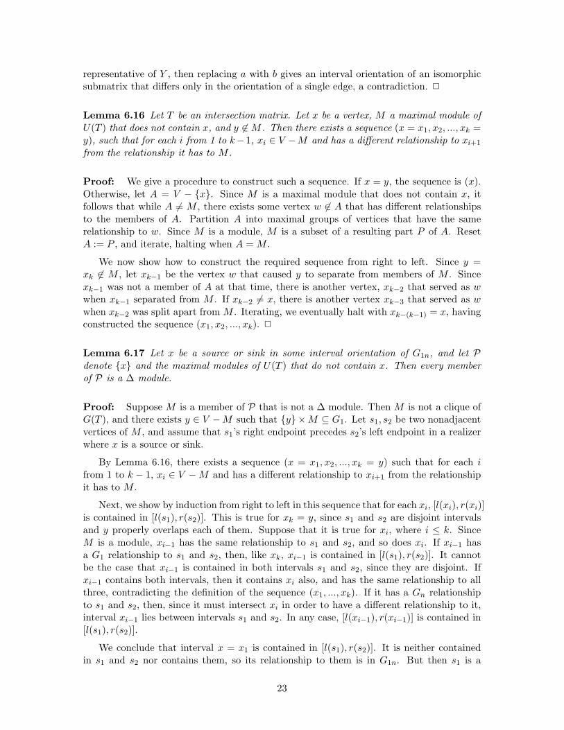
Lemma 6.16 Let T be an intersection matrix. Let x be a vertex, M a maximal module ofU(T ) that does not contain x, and y 6∈ M . Then there exists a sequence (x = x1, x2, ..., xk =y), such that for each i from 1 to k−1, xi ∈ V −M and has a different relationship to xi+1

from the relationship it has to M .

Proof: We give a procedure to construct such a sequence. If x = y, the sequence is (x).Otherwise, let A = V − x. Since M is a maximal module that does not contain x, itfollows that while A 6= M , there exists some vertex w 6∈ A that has different relationshipsto the members of A. Partition A into maximal groups of vertices that have the samerelationship to w. Since M is a module, M is a subset of a resulting part P of A. ResetA := P , and iterate, halting when A = M .

We now show how to construct the required sequence from right to left. Since y =xk 6∈ M , let xk−1 be the vertex w that caused y to separate from members of M . Sincexk−1 was not a member of A at that time, there is another vertex, xk−2 that served as wwhen xk−1 separated from M . If xk−2 6= x, there is another vertex xk−3 that served as wwhen xk−2 was split apart from M . Iterating, we eventually halt with xk−(k−1) = x, havingconstructed the sequence (x1, x2, ..., xk). 2

Lemma 6.17 Let x be a source or sink in some interval orientation of G1n, and let Pdenote x and the maximal modules of U(T ) that do not contain x. Then every memberof P is a ∆ module.

Proof: Suppose M is a member of P that is not a ∆ module. Then M is not a clique ofG(T ), and there exists y ∈ V −M such that y ×M ⊆ G1. Let s1, s2 be two nonadjacentvertices of M , and assume that s1’s right endpoint precedes s2’s left endpoint in a realizerwhere x is a source or sink.

By Lemma 6.16, there exists a sequence (x = x1, x2, ..., xk = y) such that for each ifrom 1 to k − 1, xi ∈ V −M and has a different relationship to xi+1 from the relationshipit has to M .

Next, we show by induction from right to left in this sequence that for each xi, [l(xi), r(xi)]is contained in [l(s1), r(s2)]. This is true for xk = y, since s1 and s2 are disjoint intervalsand y properly overlaps each of them. Suppose that it is true for xi, where i ≤ k. SinceM is a module, xi−1 has the same relationship to s1 and s2, and so does xi. If xi−1 hasa G1 relationship to s1 and s2, then, like xk, xi−1 is contained in [l(s1), r(s2)]. It cannotbe the case that xi−1 is contained in both intervals s1 and s2, since they are disjoint. Ifxi−1 contains both intervals, then it contains xi also, and has the same relationship to allthree, contradicting the definition of the sequence (x1, ..., xk). If it has a Gn relationshipto s1 and s2, then, since it must intersect xi in order to have a different relationship to it,interval xi−1 lies between intervals s1 and s2. In any case, [l(xi−1), r(xi−1)] is contained in[l(s1), r(s2)].

We conclude that interval x = x1 is contained in [l(s1), r(s2)]. It is neither containedin s1 and s2 nor contains them, so its relationship to them is in G1n. But then s1 is a

23

predecessor of x and s2 is a successor of x in the corresponding interval orientation of G1n.Therefore, x cannot be a source or source or sink in any interval orientation of G1n, acontradiction. 2

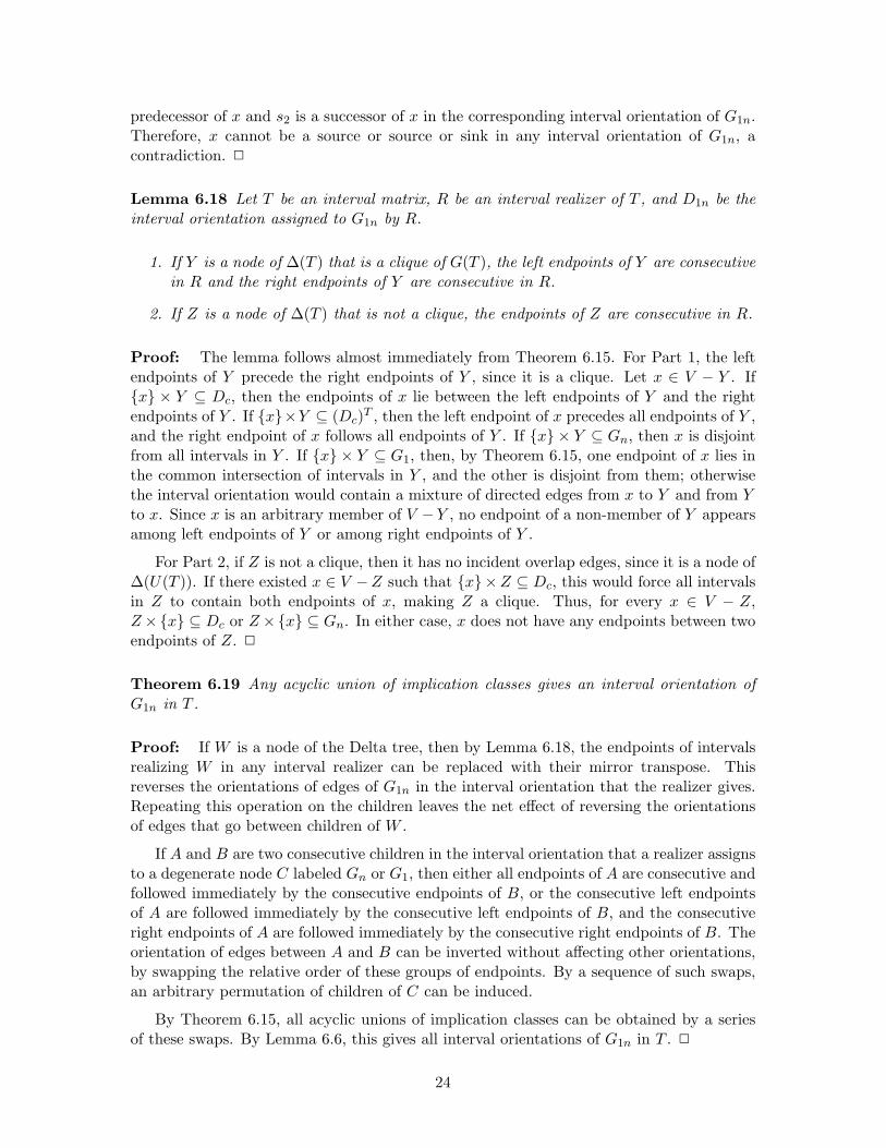
Lemma 6.18 Let T be an interval matrix, R be an interval realizer of T , and D1n be theinterval orientation assigned to G1n by R.

1. If Y is a node of ∆(T ) that is a clique of G(T ), the left endpoints of Y are consecutivein R and the right endpoints of Y are consecutive in R.

2. If Z is a node of ∆(T ) that is not a clique, the endpoints of Z are consecutive in R.

Proof: The lemma follows almost immediately from Theorem 6.15. For Part 1, the leftendpoints of Y precede the right endpoints of Y , since it is a clique. Let x ∈ V − Y . Ifx × Y ⊆ Dc, then the endpoints of x lie between the left endpoints of Y and the rightendpoints of Y . If x×Y ⊆ (Dc)T , then the left endpoint of x precedes all endpoints of Y ,and the right endpoint of x follows all endpoints of Y . If x × Y ⊆ Gn, then x is disjointfrom all intervals in Y . If x × Y ⊆ G1, then, by Theorem 6.15, one endpoint of x lies inthe common intersection of intervals in Y , and the other is disjoint from them; otherwisethe interval orientation would contain a mixture of directed edges from x to Y and from Yto x. Since x is an arbitrary member of V −Y , no endpoint of a non-member of Y appearsamong left endpoints of Y or among right endpoints of Y .

For Part 2, if Z is not a clique, then it has no incident overlap edges, since it is a node of∆(U(T )). If there existed x ∈ V −Z such that x×Z ⊆ Dc, this would force all intervalsin Z to contain both endpoints of x, making Z a clique. Thus, for every x ∈ V − Z,Z×x ⊆ Dc or Z×x ⊆ Gn. In either case, x does not have any endpoints between twoendpoints of Z. 2

Theorem 6.19 Any acyclic union of implication classes gives an interval orientation ofG1n in T .

Proof: If W is a node of the Delta tree, then by Lemma 6.18, the endpoints of intervalsrealizing W in any interval realizer can be replaced with their mirror transpose. Thisreverses the orientations of edges of G1n in the interval orientation that the realizer gives.Repeating this operation on the children leaves the net effect of reversing the orientationsof edges that go between children of W .

If A and B are two consecutive children in the interval orientation that a realizer assignsto a degenerate node C labeled Gn or G1, then either all endpoints of A are consecutive andfollowed immediately by the consecutive endpoints of B, or the consecutive left endpointsof A are followed immediately by the consecutive left endpoints of B, and the consecutiveright endpoints of A are followed immediately by the consecutive right endpoints of B. Theorientation of edges between A and B can be inverted without affecting other orientations,by swapping the relative order of these groups of endpoints. By a sequence of such swaps,an arbitrary permutation of children of C can be induced.

By Theorem 6.15, all acyclic unions of implication classes can be obtained by a seriesof these swaps. By Lemma 6.6, this gives all interval orientations of G1n in T . 2

24

Johnson and Spinrad have independently developed an idea that is related to the ∆tree [15]. Their tree, which they call an MD-PQ tree, has 2n leaves instead of n leaves, andeach leaf represents an endpoint of an interval in a realizer of G, rather than a vertex. Theset of permutations of the leaves represented by a set of allowable reorderings of childrenof nodes on the tree represents all realizers of G, rather than realizers of an intersectionmatrix.

6.4 An algorithm for finding a realizer of an interval matrix

The approach works by finding an interval orientation of G1n and then finding the corre-sponding interval realizer. This requires us to give solutions to the following:

Problem 1: Given a topological sort of an interval orientation of G1n, find the correspond-ing interval realizer.

Problem 2: Find a topological sort of an interval orientation of G1n.

Our algorithm is a variant of the transitive orientation algorithm of [18]. That algorithmuses the Γ relation to constrain the orientation it produces. We adapt the algorithm to usethe ∆ relation instead of the Γ relation to constrain the orientation.

6.4.1 Problem 1: Given an interval orientation, find the corresponding intervalrealizer

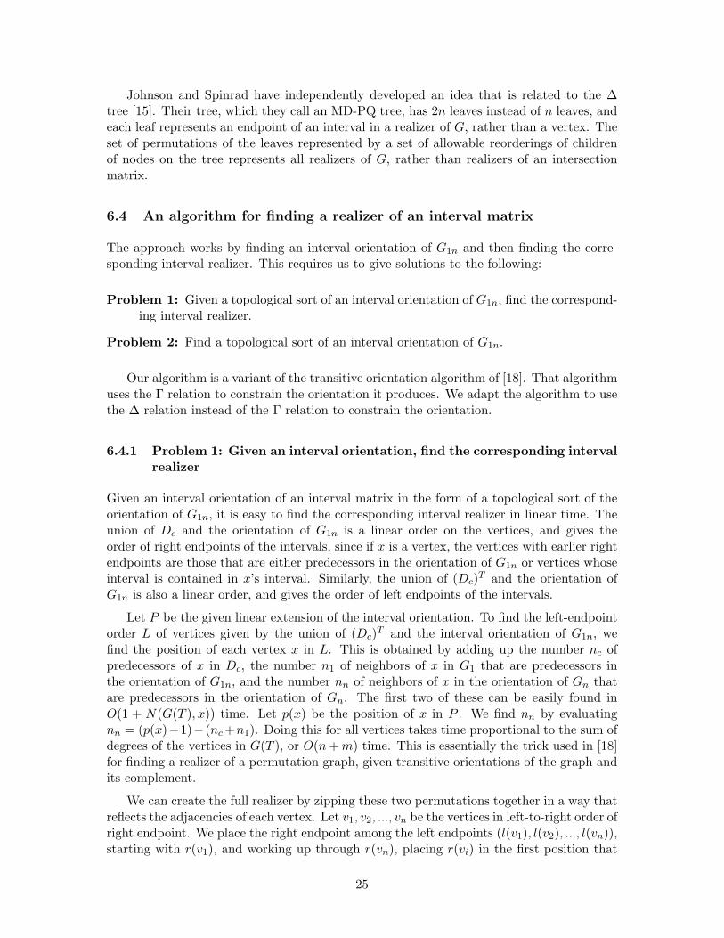
Given an interval orientation of an interval matrix in the form of a topological sort of theorientation of G1n, it is easy to find the corresponding interval realizer in linear time. Theunion of Dc and the orientation of G1n is a linear order on the vertices, and gives theorder of right endpoints of the intervals, since if x is a vertex, the vertices with earlier rightendpoints are those that are either predecessors in the orientation of G1n or vertices whoseinterval is contained in x’s interval. Similarly, the union of (Dc)T and the orientation ofG1n is also a linear order, and gives the order of left endpoints of the intervals.

Let P be the given linear extension of the interval orientation. To find the left-endpointorder L of vertices given by the union of (Dc)T and the interval orientation of G1n, wefind the position of each vertex x in L. This is obtained by adding up the number nc ofpredecessors of x in Dc, the number n1 of neighbors of x in G1 that are predecessors inthe orientation of G1n, and the number nn of neighbors of x in the orientation of Gn thatare predecessors in the orientation of Gn. The first two of these can be easily found inO(1 + N(G(T ), x)) time. Let p(x) be the position of x in P . We find nn by evaluatingnn = (p(x)−1)− (nc +n1). Doing this for all vertices takes time proportional to the sum ofdegrees of the vertices in G(T ), or O(n + m) time. This is essentially the trick used in [18]for finding a realizer of a permutation graph, given transitive orientations of the graph andits complement.

We can create the full realizer by zipping these two permutations together in a way thatreflects the adjacencies of each vertex. Let v1, v2, ..., vn be the vertices in left-to-right order ofright endpoint. We place the right endpoint among the left endpoints (l(v1), l(v2), ..., l(vn)),starting with r(v1), and working up through r(vn), placing r(vi) in the first position that

25

is both to the right of r(vi−1) and to the right of the rightmost left endpoint of neighborsof vi.

6.4.2 Overview of solution to Problem 2: finding an interval orientation of aninterval matrix

Recall that we are required only to give a topological sort of G1n. This saves us from havingto orient edges of Gn explicitly, which would violate the time bound.

The basic operation begins with an partition P of the vertices and refines the partitionclasses until every partition class is a ∆ module. It does this in a way that avoids splittingapart members of any ∆ module that is initially a subset of a class of P. The final partitiontherefore gives the maximal ∆ modules that were initially subsets of classes of P.

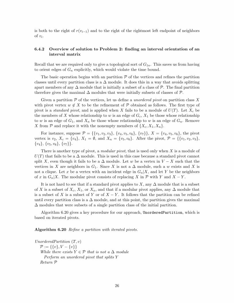
Given a partition P of the vertices, let us define a unordered pivot on partition class Xwith pivot vertex w 6∈ X to be the refinement of P obtained as follows. The first type ofpivot is a standard pivot, and is applied when X fails to be a module of U(T ). Let Xc bethe members of X whose relationship to w is an edge of Gc, X1 be those whose relationshipto w is an edge of G1, and Xn be those whose relationship to w is an edge of Gn. RemoveX from P and replace it with the nonempty members of Xc, X1, Xn.

For instance, suppose P = v1, v2, v3, v4, v5, v6, v7, X = v4, v5, v6, the pivotvertex is v2, Xc = v4, X1 = ∅, and Xn = v5, v6. After the pivot, P = v1, v2, v3,v4, v5, v6, v7.

There is another type of pivot, a modular pivot, that is used only when X is a module ofU(T ) that fails to be a ∆ module. This is used in this case because a standard pivot cannotsplit X, even though it fails to be a ∆ module. Let w be a vertex in V −X such that thevertices in X are neighbors in G1. Since X is not a ∆ module, such a w exists and X isnot a clique. Let x be a vertex with an incident edge in Gn|X, and let Y be the neighborsof x in Gn|X. The modular pivot consists of replacing X in P with Y and X − Y .

It is not hard to see that if a standard pivot applies to X, any ∆ module that is a subsetof X is a subset of Xc, X1, or Xn, and that if a modular pivot applies, any ∆ module thatis a subset of X is a subset of Y or of X − Y . It follows that the partition can be refineduntil every partition class is a ∆ module, and at this point, the partition gives the maximal∆ modules that were subsets of a single partition class of the initial partition.

Algorithm 6.20 gives a key procedure for our approach, UnorderedPartition, which isbased on iterated pivots.

Algorithm 6.20 Refine a partition with iterated pivots.

UnorderedPartition (T, v)P := v, V − vWhile there exists Y ∈ P that is not a ∆ module

Perform an unordered pivot that splits YReturn P

26

Let us now modify UnorderedPartition so that it maintains an ordering on the parti-tion classes of P as it refines it. Initially, the ordering is (v, V − v).

When X is split with a pivot on w, we keep track of the spot formerly occupied by Xin the linear order. When Xc, X1, and Xn are inserted, they are inserted consecutivelyat that spot. Their relative order within that spot is determined as follows. If w lies in apartition class that precedes X’s spot, then their relative order is (Xc, X1, Xn); otherwise itis (Xn, X1, Xc). In the case of a modular pivot, we place X − Y first if the pivot w residesin a class that is later in the ordering than X, and place it second if the pivot resides in anearlier class.

We may call this ordered variant Partition. Henceforth in the paper, we will refer tothis (ordered) pivot when we use the term “pivot”.

Let us say an ordering of partition classes on V is consistent with an interval orientationif all arcs in the orientation that go between partition classes are oriented from earlier tolater partition classes in the order.

To explore the key insights in a simple setting, let us suppose that T is an intervalmatrix and U(T ) is ∆ prime. Suppose also that we know a vertex v that is a source insome interval orientation D1n of G1n. Then the initial ordered partition (v, V − v)is consistent with D1n. Moreover, it is easy to see by induction on the number of pivotsthat every successive refinement is consistent with the interval orientation. The reason forthis is that after a standard pivot, the set E′ of edges of G1n that go between membersof Xc, X1, Xn have a ∆ relationship to the set E′′ of edges that are incident to both Xand the pivot vertex w. By induction, edges in E′′ are all oriented toward X in D1n if w isin an earlier class than X in the ordering on P, or all oriented toward w if w is in a laterclass. Consider the relative ordering of Xc, X1, Xn as (Xc, X1, Xn) or (Xn, X1, Xc). The∆ relationships between E′ and E′′ force members of E′ to be oriented to the right in thisordering, which means that the induction hypothesis remains true after the pivot.

For instance, suppose that w precedes X. Let ab be an edge of G1n such that a ∈ Xc

and b ∈ X1. Then wa ∈ Gc, wb ∈ G1, and ab ∈ G1n, hence (a, b)∆(w, b). Since w precedesb, we may assume by induction that (w, b) is in D1n, so (a, b) is also in D1n.

A similar analysis applies when a ∈ X1, b ∈ Xn, or a ∈ Xc and b ∈ Xn. We showbelow that modular pivots also maintain the invariant that the ordered partition remainsconsistent with the interval orientation.

Since U(T ) is ∆ prime, it has only trivial modules. Thus, all partition classes aresingletons when the procedure halts. Since the ordering on these is consistent with aninterval orientation, their ordering is a topological sort of D1n. This topological sort,together with the representation of G1n given by T , gives a representation of D1n that isadequate for our purposes.

To get this solution, we assumed above that v was a source in an interval orientationin order to ensure that the induction hypothesis was true initially. It remains to establishhow to find v. Somewhat surprisingly, v may be found by the same procedure. Selectingan arbitrary vertex u, and starting Partition with initial partition (u, V − u) yieldsan ordering on the vertices as before. The last vertex v in this ordering is a source in anyinterval orientation that orients vu as (v, u). This is shown by a similar induction. Theinduction hypothesis this time is that as the partition is refined, all edges of G1n from v to

27

vertices outside of v’s current partition class in P are oriented away from v. This is trueinitially when the only such edge is vu.

By these observations, Algorithm 6.21 gives a procedure for producing a topological sortof an interval orientation when U(T ) is prime.

Algorithm 6.21 Find a topological sort of an interval orientation of G1n when U(T ) isprime.

OrientPrime (T)Select arbitrary vertex uP1 = Partition (T, u)Let v be the member of the rightmost class in P1

P := Partition (T, v)Return P as the topological sort

Let us now relax the assumption that U(T ) is ∆ prime and generalize this procedureto obtain a general solution to our problem. Partition(T, v) has no way to break apartany ∆ modules of U(T ) that are contained in V − v. Instead, it may halt with somepartition classes that are non-singleton ∆ modules. Thus, the final ordering of partitionclasses leaves unspecified the order on the vertices that are contained inside such a module.

The way we get around this is to start up the partitioning process recursively insidesuch a ∆ module in order to complete the ordering. The algorithm then makes two callsto this recursive variant, RPartition, in place of two calls to Partition. Algorithm 6.22gives the algorithm, with RPartition implemented as an iterative procedure that makes aseries of calls to Partition.

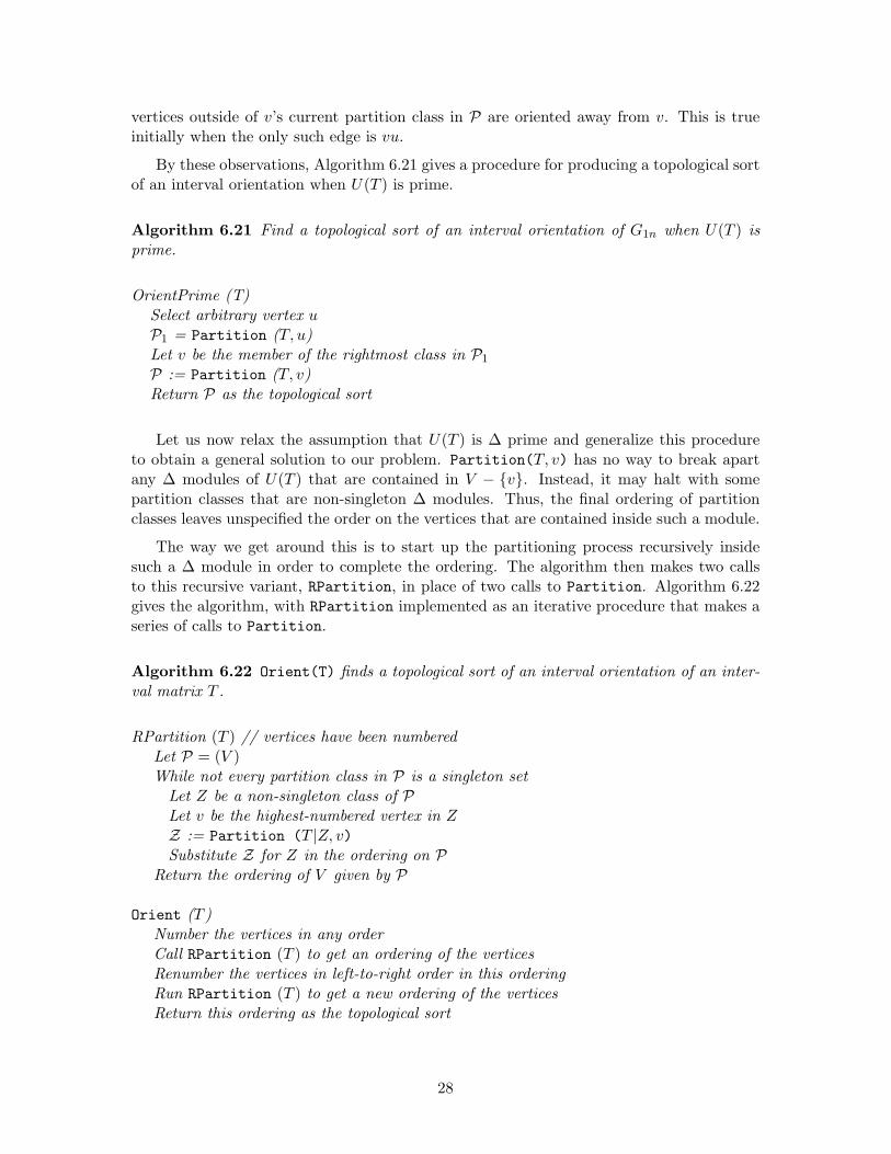
Algorithm 6.22 Orient(T) finds a topological sort of an interval orientation of an inter-val matrix T .

RPartition (T ) // vertices have been numberedLet P = (V )While not every partition class in P is a singleton set

Let Z be a non-singleton class of PLet v be the highest-numbered vertex in ZZ := Partition (T |Z, v)Substitute Z for Z in the ordering on P

Return the ordering of V given by P

Orient (T )Number the vertices in any orderCall RPartition (T ) to get an ordering of the verticesRenumber the vertices in left-to-right order in this orderingRun RPartition (T ) to get a new ordering of the verticesReturn this ordering as the topological sort

28

We show below that in the second call to RPartition from Orient, the highest-numbered vertex in a Z in the loop is a source in an interval orientation of G1n|Z. We alsoshow that Z is a ∆ module. Therefore, we do not need to worry about interactions betweenorientations of edges of G1n|Z and other edges of G1n in assigning an interval orientationto them; the call to Partition(T |Z, v) does not need to take the rest of P into account inmaintaining the invariant that the ordering on P is consistent with an interval orientation.The procedure halts when all partition classes are singletons, and at this point, the orderon them will be a topological sort of an interval orientation of G1n.

6.4.3 Proof of correctness of Algorithm 6.22

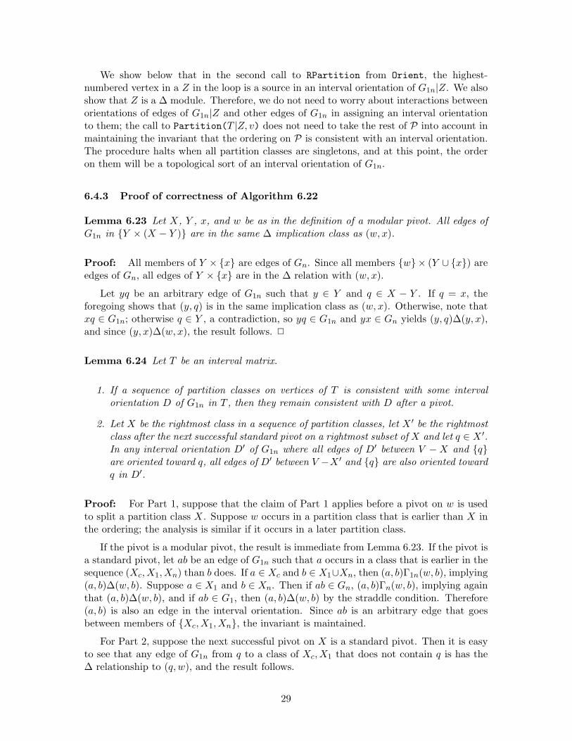
Lemma 6.23 Let X, Y , x, and w be as in the definition of a modular pivot. All edges ofG1n in Y × (X − Y ) are in the same ∆ implication class as (w, x).

Proof: All members of Y × x are edges of Gn. Since all members w × (Y ∪ x) areedges of Gn, all edges of Y × x are in the ∆ relation with (w, x).

Let yq be an arbitrary edge of G1n such that y ∈ Y and q ∈ X − Y . If q = x, theforegoing shows that (y, q) is in the same implication class as (w, x). Otherwise, note thatxq ∈ G1n; otherwise q ∈ Y , a contradiction, so yq ∈ G1n and yx ∈ Gn yields (y, q)∆(y, x),and since (y, x)∆(w, x), the result follows. 2

Lemma 6.24 Let T be an interval matrix.

1. If a sequence of partition classes on vertices of T is consistent with some intervalorientation D of G1n in T , then they remain consistent with D after a pivot.

2. Let X be the rightmost class in a sequence of partition classes, let X ′ be the rightmostclass after the next successful standard pivot on a rightmost subset of X and let q ∈ X ′.In any interval orientation D′ of G1n where all edges of D′ between V −X and qare oriented toward q, all edges of D′ between V −X ′ and q are also oriented towardq in D′.

Proof: For Part 1, suppose that the claim of Part 1 applies before a pivot on w is usedto split a partition class X. Suppose w occurs in a partition class that is earlier than X inthe ordering; the analysis is similar if it occurs in a later partition class.

If the pivot is a modular pivot, the result is immediate from Lemma 6.23. If the pivot isa standard pivot, let ab be an edge of G1n such that a occurs in a class that is earlier in thesequence (Xc, X1, Xn) than b does. If a ∈ Xc and b ∈ X1∪Xn, then (a, b)Γ1n(w, b), implying(a, b)∆(w, b). Suppose a ∈ X1 and b ∈ Xn. Then if ab ∈ Gn, (a, b)Γn(w, b), implying againthat (a, b)∆(w, b), and if ab ∈ G1, then (a, b)∆(w, b) by the straddle condition. Therefore(a, b) is also an edge in the interval orientation. Since ab is an arbitrary edge that goesbetween members of Xc, X1, Xn, the invariant is maintained.

For Part 2, suppose the next successful pivot on X is a standard pivot. Then it is easyto see that any edge of G1n from q to a class of Xc, X1 that does not contain q is has the∆ relationship to (q, w), and the result follows.

29

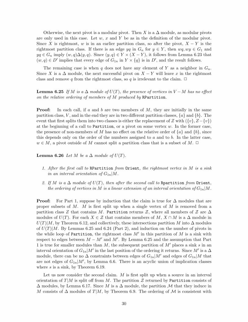
Otherwise, the next pivot is a modular pivot. Then X is a ∆ module, as modular pivotsare only used in this case. Let w, x and Y be as in the definition of the modular pivot.Since X is rightmost, w is in an earlier partition class, so after the pivot, X − Y is therightmost partition class. If there is an edge yq in Gn for y ∈ Y , then wq, wy ∈ G1 andyq ∈ Gn imply (w, q)∆(y, q). Since (y, q) ∈ Y × (X − Y ), it follows from Lemma 6.23 that(w, q) ∈ D′ implies that every edge of G1n in Y × q is in D′, and the result follows.

The remaining case is when q does not have any element of Y as a neighbor in Gn.Since X is a ∆ module, the next successful pivot on X − Y will leave x in the rightmostclass and remove q from the rightmost class, so q is irrelevant to the claim. 2

Lemma 6.25 If M is a ∆ module of U(T ), the presence of vertices in V −M has no effecton the relative ordering of members of M produced by RPartition.

Proof: In each call, if a and b are two members of M , they are initially in the samepartition class, V , and in the end they are in two different partition classes, a and b. Theevent that first splits them into two classes is either the replacement of Z with (v, Z−v)at the beginning of a call to Partition, or a pivot on some vertex w. In the former case,the presence of non-members of M has no effect on the relative order of a and b, sincethis depends only on the order of the numbers assigned to a and to b. In the latter case,w ∈ M , a pivot outside of M cannot split a partition class that is a subset of M . 2

Lemma 6.26 Let M be a ∆ module of U(T ).

1. After the first call to RPartition from Orient, the rightmost vertex in M is a sinkin an interval orientation of G1n|M .

2. If M is a ∆ module of U(T ), then after the second call to Rpartition from Orient,the ordering of vertices in M is a linear extension of an interval orientation of G1n|M .

Proof: For Part 1, suppose by induction that the claim is true for ∆ modules that areproper subsets of M . M is first split up when a single vertex of M is removed from apartition class Z that contains M . Partition returns Z, where all members of Z are ∆modules of U(T ). For each X ∈ Z that contains members of M , X ∩M is a ∆ module inU(T )|M , by Theorem 6.12, and collectively, these intersections partition M into ∆ modulesof U(T )|M . By Lemmas 6.25 and 6.24 (Part 2), and induction on the number of pivots inthe while loop of Partition, the rightmost class M ′ in this partition of M is a sink withrespect to edges between M −M ′ and M ′. By Lemma 6.25 and the assumption that Part1 is true for smaller modules than M , the subsequent partition of M ′ places a sink s in aninterval orientation of G1n|M ′ in the last position of the ordering it returns. Since M ′ is a ∆module, there can be no ∆ constraints between edges of G1n|M ′ and edges of G1n|M thatare not edges of G1n|M ′, by Lemma 6.6. There is an acyclic union of implication classeswhere s is a sink, by Theorem 6.19.

Let us now consider the second claim. M is first split up when a source in an intervalorientation of T |M is split off from M . The partition Z returned by Partition consists of∆ modules, by Lemma 6.17. Since M is a ∆ module, the partition M that they induce inM consists of ∆ modules of T |M , by Theorem 6.9. The ordering of M is consistent with

30

an interval orientation of T |M , by Lemmas 6.24 and 6.25. By induction on the size of a∆ module, the remaining pivots produce interval orientations of each member of M, andsince they are ∆ modules, these orientations can be combined with the ordering on M togive an interval orientation of T |M , by Theorem 6.19. 2

Since V is a ∆ module, the second call to RPartition produces a linear extension ofan interval orientation. Once RPartition is run, an interval realizer may be constructedand checked in linear time, using Algorithm 5.1. The bottleneck for the time bound is therunning time of RPartition.

6.4.4 An O(n + m log n)-time implementation

We have already shown that the time to construct a realizer of an interval matrix is givenby the running time of RPartition on the matrix. The first call to RPartition in Algo-rithm 6.22 serves only to partition the rightmost class in the ordering. Performing onlypivots on the rightmost class until it is a singleton set takes O(n+m) time, since it requiresone pivot on each vertex after it leaves the rightmost class. The second call to RPartitiondoes not require any modular pivots, by Lemma 6.17. Thus, in obtaining the time bound,we may focus only on the second call and assume that all pivots are standard pivots.

Algorithm 6.27 gives an implementation of the while loop of RPartition that allowsRPartition to run in O(n+m log n) time. The algorithm is similar to the approach of [19]and [13]. Retrieving E′ takes time proportional to the sum of degrees of X. The groupingoperations on E′ take O(|E′|) time, by distributing the edges to buckets that are initiallyempty, and maintaining a list of nonempty buckets to allow retrieval of the groups withoutvisiting empty buckets, leaving the buckets empty again. The selection of X ensures thateach time a vertex is used as a pivot, the partition class that currently contains it is at mosthalf as large as the class that contained it the last time it was used as a pivot. A vertex istherefore used O(log n) times as a pivot. A pivot on x requires O(|N(x)|) time, giving thebound.

This clever idea is due to Spinrad, and initially appeared in an unpublished but influen-tial manuscript, which he has circulated beginning in 1985 [26]. This paper was also the firstto propose vertex partitioning as an algorithmic tool, and to recognize its importance to themodular decomposition and transitive orientation problems. Algorithm 6.27 is a variationof his time-bound argument that bounds the cost of partitioning inside all recursive callsto RPartition, instead of just in the main loop.

Algorithm 6.27 Vertex partitioning.

Partition (G, P)If |P| = 1 return Pelse

Let X be a member of P that is not larger than all othersLet E′ be the edges of G in X × (V (G)−X).Group members of E′ by endpoint in XUse each x ∈ X as a pivot on all partition classes in V −XRegroup members of E′ by endpoint in V −X

31

Use each v ∈ V − x as a pivot on all partition classes in XLet Q be the classes of P ′ now contained in XLet Q′ be the classes of P ′ now contained in V (G)−XReturn Partition(G|X,Q) ∪ Partition(G−X,Q′)

Because of its simplicity, it would be the method of choice in a practical implementationof the algorithm of this paper, in our view. This is a bottleneck in the circular-arc graphrecognition algorithm. To get a linear time bound for recognizing circular-arc graphs weneed a linear bound for RPartition. To do this we use a considerably more complicatedstrategy, which we give below. Before we do that, we show how RPartition can be usedto obtain the ∆ tree.

6.4.5 Linear-time implementation

From a theoretical standpoint, an O(n+m log n) bound for RPartition would be a bottle-neck in our circular-arc graph recognition algorithm, and would result in an O(n+m log n)bound for it also.

To get a linear bound, we must make use of the considerably more difficult linear-timeapproach to vertex partitioning that is given in [18]. In this section, we prove the following:

Theorem 6.28 RPartition can be carried out in O(n + m) time.

This is the most difficult part of the paper, since it requires a summary descriptionof tricks that are explained in greater detail in [18]. There is no loss of continuity if oneaccepts Theorem 6.28 provisionally on a first reading and skips to Section 8.

The following are given in [18]:

Theorem 6.29 Let G be a prime graph, and let P be an arbitrary initial partition of V .Partition may be implemented so that it takes O(n + m) time to halt with all partitionclasses singletons.

Theorem 6.30 It takes linear time to find the modular decomposition of an undirectedgraph.

By Theorem 6.29, it is immediate that we can run Partition in linear time on a primegraph; RPartition partitions V down to singleton sets. The paper solves the general tran-sitive orientation problem through a reduction to prime graphs. In addition, the algorithmis specific to undirected graphs, and it is not immediate that it can be generalized even toprime interval matrices. For our application, we must be able to run RPartition on U(T ),where T is an interval matrix that need not be prime, and still get a linear time bound forRPartition.

We develop our algorithm in two steps. In the first, we show how to perform RPartitionon an undirected graph that need not be prime, in linear time, and in the second, we showhow to do it on U(T ), where U(T ) need not be prime.

32

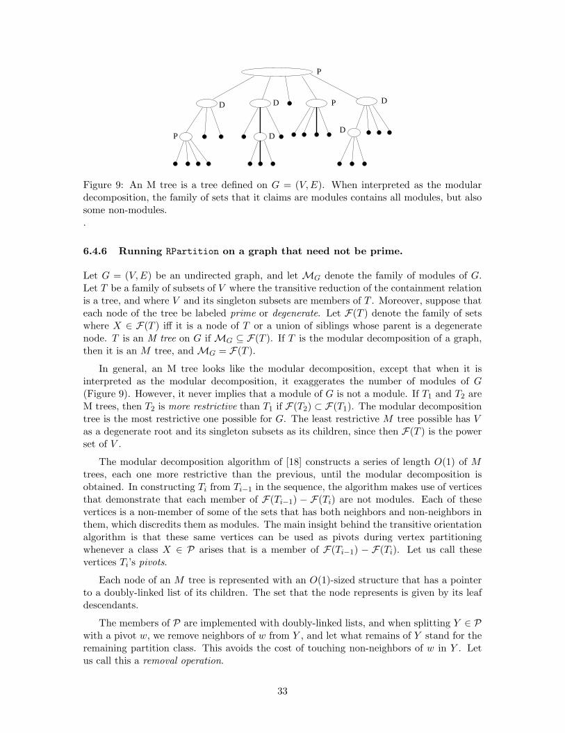
DDD P

D

P

PD

Figure 9: An M tree is a tree defined on G = (V,E). When interpreted as the modulardecomposition, the family of sets that it claims are modules contains all modules, but alsosome non-modules..

6.4.6 Running RPartition on a graph that need not be prime.

Let G = (V,E) be an undirected graph, and let MG denote the family of modules of G.Let T be a family of subsets of V where the transitive reduction of the containment relationis a tree, and where V and its singleton subsets are members of T . Moreover, suppose thateach node of the tree be labeled prime or degenerate. Let F(T ) denote the family of setswhere X ∈ F(T ) iff it is a node of T or a union of siblings whose parent is a degeneratenode. T is an M tree on G if MG ⊆ F(T ). If T is the modular decomposition of a graph,then it is an M tree, and MG = F(T ).

In general, an M tree looks like the modular decomposition, except that when it isinterpreted as the modular decomposition, it exaggerates the number of modules of G(Figure 9). However, it never implies that a module of G is not a module. If T1 and T2 areM trees, then T2 is more restrictive than T1 if F(T2) ⊂ F(T1). The modular decompositiontree is the most restrictive one possible for G. The least restrictive M tree possible has Vas a degenerate root and its singleton subsets as its children, since then F(T ) is the powerset of V .

The modular decomposition algorithm of [18] constructs a series of length O(1) of Mtrees, each one more restrictive than the previous, until the modular decomposition isobtained. In constructing Ti from Ti−1 in the sequence, the algorithm makes use of verticesthat demonstrate that each member of F(Ti−1) − F(Ti) are not modules. Each of thesevertices is a non-member of some of the sets that has both neighbors and non-neighbors inthem, which discredits them as modules. The main insight behind the transitive orientationalgorithm is that these same vertices can be used as pivots during vertex partitioningwhenever a class X ∈ P arises that is a member of F(Ti−1) − F(Ti). Let us call thesevertices Ti’s pivots.

Each node of an M tree is represented with an O(1)-sized structure that has a pointerto a doubly-linked list of its children. The set that the node represents is given by its leafdescendants.

The members of P are implemented with doubly-linked lists, and when splitting Y ∈ Pwith a pivot w, we remove neighbors of w from Y , and let what remains of Y stand for theremaining partition class. This avoids the cost of touching non-neighbors of w in Y . Letus call this a removal operation.

33

Lemma 6.31 [18] (See Figure 9) Given an M tree T on graph G, one may perform thefollowing in time linear in the size of G:

1. Sort all adjacency lists so that the neighbors of each vertex x are given in order oftheir left-to-right appearance as leaves of T . For each node of the tree, the membersof the node are therefore consecutive in the adjacency list of x.

2. Label each node U of the tree with a sorted list SN(U) of vertices in V − U thatare adjacent to all members of U . SN(U) is sorted in left-to-right appearance of itsmembers as leaves of T , and the sum of lengths of these lists is linear in the size ofG.

3. Label each node U that is not a module with the leftmost vertex l(U) ∈ V − U andrightmost r(U) ∈ V − U that is adjacent to some members of U and nonadjacent toothers; since U is not a module, at least one of these is defined. Let s(U) denoteone of them. U is also equipped with a pointer to the consecutive interval occupied byN(s(U)) ∩ U in s(U)’s adjacency list.

The algorithm assigns a private copy of an adjacency-list representation of G to each Ti,and applies Lemma 6.31 to each. It uses a restarting procedure on each Ti, which initiatespivots on P, halting only when P ⊆ F(Ti). (See Figure 10.) To do this, it makes a callto the restarting procedure on Ti−1. When that restarting procedure halts, it makes use ofTi’s pivots to split some classes, communicates these splits to Ti−1 as capricious splits, andthen calls the restarting procedure on Ti−1 to get the partitioning restarted. The procedurefails to find any pivots to restart partitioning only if P ⊆ F(Ti), in which case it is allowedto halt.

The restarting procedure is linear if it may be restarted O(n+m) times without spendingmore than O(n + m) total time, including the time to perform the pivots it generates andto maintain the list of unprocessed nodes. All of the restarting procedures in the sequenceof M trees are linear ones.

Notice that a linear restarting procedure on the last tree in the sequence, MD(G),would suffice for a linear-time implementation of RPartition. The restarting procedurecould perform the while loop of Partition, halting when every partition class is a memberof F(MD(G)) (i.e. a module). A new call to Partition(T |Z, v) could then initiate thesplit (v, Z) of a module Z and restart the restarting procedure again. By the definitionof a linear restarting procedure, the time for all calls to the restarting procedure would belinear.

General linear restarting procedures are given in [18] for all trees in the sequence exceptfor the very last one, which is the modular decomposition of G. This is unfortunate, sincedoing this requires only a straightforward extension of the techniques used for the otherrestarting procedures, which must now be resurrected here. The reason that this wasnot done is that when the modular decomposition is available, transitive orientation of acomparability graph reduces to transitive orientation of prime graphs, and this step wasunnecessary for transitive orientation.

The reason pivoting risks being wasteful is that the class that contains a pivot vertex xcannot be split by x, so time might be wasted traversing members of x’s class in splitting up

34

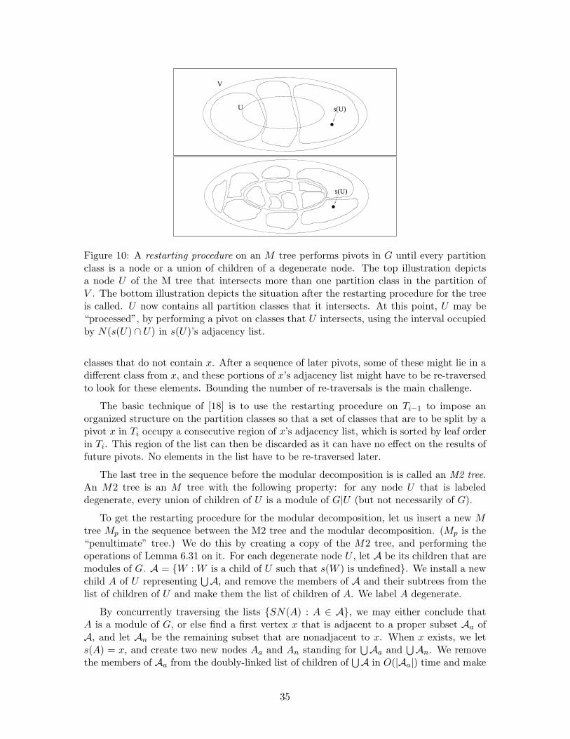
U

V

s(U)

s(U)

Figure 10: A restarting procedure on an M tree performs pivots in G until every partitionclass is a node or a union of children of a degenerate node. The top illustration depictsa node U of the M tree that intersects more than one partition class in the partition ofV . The bottom illustration depicts the situation after the restarting procedure for the treeis called. U now contains all partition classes that it intersects. At this point, U may be“processed”, by performing a pivot on classes that U intersects, using the interval occupiedby N(s(U) ∩ U) in s(U)’s adjacency list.

classes that do not contain x. After a sequence of later pivots, some of these might lie in adifferent class from x, and these portions of x’s adjacency list might have to be re-traversedto look for these elements. Bounding the number of re-traversals is the main challenge.

The basic technique of [18] is to use the restarting procedure on Ti−1 to impose anorganized structure on the partition classes so that a set of classes that are to be split by apivot x in Ti occupy a consecutive region of x’s adjacency list, which is sorted by leaf orderin Ti. This region of the list can then be discarded as it can have no effect on the results offuture pivots. No elements in the list have to be re-traversed later.

The last tree in the sequence before the modular decomposition is is called an M2 tree.An M2 tree is an M tree with the following property: for any node U that is labeleddegenerate, every union of children of U is a module of G|U (but not necessarily of G).

To get the restarting procedure for the modular decomposition, let us insert a new Mtree Mp in the sequence between the M2 tree and the modular decomposition. (Mp is the“penultimate” tree.) We do this by creating a copy of the M2 tree, and performing theoperations of Lemma 6.31 on it. For each degenerate node U , let A be its children that aremodules of G. A = W : W is a child of U such that s(W ) is undefined. We install a newchild A of U representing

⋃A, and remove the members of A and their subtrees from the

list of children of U and make them the list of children of A. We label A degenerate.

By concurrently traversing the lists SN(A) : A ∈ A, we may either conclude thatA is a module of G, or else find a first vertex x that is adjacent to a proper subset Aa ofA, and let An be the remaining subset that are nonadjacent to x. When x exists, we lets(A) = x, and create two new nodes Aa and An standing for

⋃Aa and

⋃An. We remove

the members of Aa from the doubly-linked list of children of⋃A in O(|Aa|) time and make

35

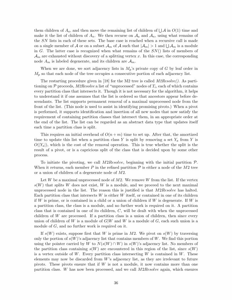
them children of Aa, and then move the remaining list of children of⋃A in O(1) time and

make it the list of children of An. We then recurse on Aa and An, using what remains ofthe SN lists in each of these sets. The base case is reached when a recursive call is madeon a single member of A or on a subset Am of A such that |Am| > 1 and

⋃Am is a module

in G. The latter case is recognized when what remains of the SN() lists of members ofAm are exhausted without discovery of a splitting vertex x. In this case, the correspondingnode Am is labeled degenerate, and its children are Am.

When we are done, we sort adjacency lists in Mp’s private copy of G by leaf order inMp so that each node of the tree occupies a consecutive portion of each adjacency list.

The restarting procedure given in [18] for the M2 tree is called M2Resolve(). As parti-tioning on P proceeds, M2Resolve a list of “unprocessed” nodes of Ti, each of which containsevery partition class that intersects it. Though it is not necessary for the algorithm, it helpsto understand it if one assumes that the list is ordered so that ancestors appear before de-scendants. The list supports permanent removal of a maximal unprocessed node from thefront of the list. (This node is used to assist in identifying promising pivots.) When a pivotis performed, it supports identification and insertion of all new nodes that now satisfy therequirement of containing partition classes that intersect them, in an appropriate order atthe end of the list. The list can be regarded as an abstract data type that updates itselfeach time a partition class is split.

This requires an initial overhead of O(n + m) time to set up. After that, the amortizedtime to update this list when a partition class Y is split by removing a set Ya from Y isO(|Ya|), which is the cost of the removal operation. This is true whether the split is theresult of a pivot, or is a capricious split of the class that is decided upon by some otherprocess.

To initiate the pivoting, we call M2Resolve, beginning with the initial partition P.When it returns, each member P in the refined partition P is either a node of the M2 treeor a union of children of a degenerate node of M2.

Let W be a maximal unprocessed node of M2. We remove W from the list. If the vertexs(W ) that splits W does not exist, W is a module, and we proceed to the next maximalunprocessed node in the list. The reason this is justified is that M2Resolve has halted.Each partition class that intersects W is either W itself, or contained in one of its childrenif W is prime, or is contained in a child or a union of children if W is degenerate. If W isa partition class, the class is a module, and no further work is required on it. A partitionclass that is contained in one of its children, C, will be dealt with when the unprocessedchildren of W are processed. If a partition class is a union of children, then since everyunion of children of W is a module of G|W and W is a module of G, each such union is amodule of G, and no further work is required on it.

If s(W ) exists, suppose first that W is prime in M2. We pivot on s(W ) by traversingonly the portion of s(W )’s adjacency list that contains members of W . We find this portionusing the pointer carried by W to N(s(W ) ∩W ) in s(W )’s adjacency list. No members ofthe partition class containing s(W ) are encountered in this region of the list, since s(W )is a vertex outside of W . Every partition class intersecting W is contained in W . Theseelements may now be discarded from W ’s adjacency list, as they are irrelevant to futurepivots. These pivots ensure that if W is not a module, it now contains more than onepartition class. W has now been processed, and we call M2Resolve again, which ensures

36

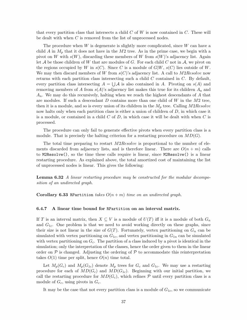
that every partition class that intersects a child C of W is now contained in C. These willbe dealt with when C is removed from the list of unprocessed nodes.

The procedure when W is degenerate is slightly more complicated, since W can have achild A in Mp that it does not have in the M2 tree. As in the prime case, we begin with apivot on W with s(W ), discarding these members of W from s(W )’s adjacency list. Againlet A be those children of W that are modules of G. For each child C not in A, we pivot onthe regions occupied by W in s(C). Since C is a module of G|W , s(C) lies outside of W .We may then discard members of W from s(C)’s adjacency list. A call to M2Resolve nowreturns with each partition class intersecting such a child C contained in C. By default,every partition class intersecting A =

⋃A is also contained in A. Pivoting on s(A) and

removing members of A from s(A)’s adjacency list makes this true for its children Aa andAn. We may do this recursively, halting when we reach the highest descendants of A thatare modules. If such a descendant D contains more than one child of W in the M2 tree,then it is a module, and so is every union of its children in the Mp tree. Calling M2Resolvenow halts only when each partition class is either a union of children of D, in which case itis a module, or contained in a child C of D, in which case it will be dealt with when C isprocessed.

The procedure can only fail to generate effective pivots when every partition class is amodule. That is precisely the halting criterion for a restarting procedure on MD(G).

The total time preparing to restart M2Resolve is proportional to the number of ele-ments discarded from adjacency lists, and is therefore linear. There are O(n + m) callsto M2Resolve(), so the time these calls require is linear, since M2Resolve() is a linearrestarting procedure. As explained above, the total amortized cost of maintaining the listof unprocessed nodes is linear. This gives the following:

Lemma 6.32 A linear restarting procedure may be constructed for the modular decompo-sition of an undirected graph.

Corollary 6.33 RPartition takes O(n + m) time on an undirected graph.

6.4.7 A linear time bound for RPartition on an interval matrix.

If T is an interval matrix, then X ⊆ V is a module of U(T ) iff it is a module of both Gn

and G1c. One problem is that we need to avoid working directly on these graphs, sincetheir size is not linear in the size of G(T ). Fortunately, vertex partitioning on Gn can besimulated with vertex partitioning on G1c, and vertex partitioning in G1n can be simulatedwith vertex partitioning on Gc. The partition of a class induced by a pivot is identical in thesimulation; only the interpretation of the classes, hence the order given to them in the linearorder on P is changed. Adjusting the ordering of P to accommodate this reinterpretationtakes O(1) time per split, hence O(n) time total.

Let Mp(Gc) and Mp(G1c) denote Mp trees for Gc and G1c. We may use a restartingprocedure for each of MD(Gc) and MD(G1c). Beginning with our initial partition, wecall the restarting procedure for MD(Gc), which refines P until every partition class is amodule of Gc, using pivots in Gc.

It may be the case that not every partition class is a module of G1c, so we communicate

37

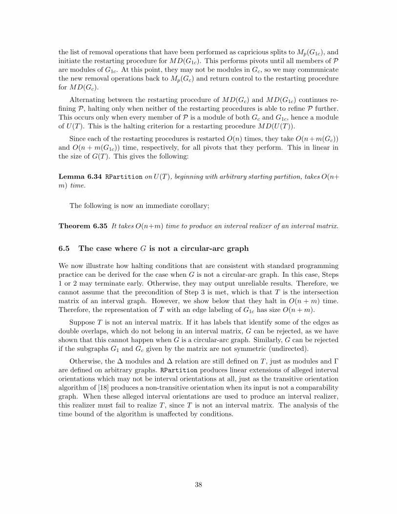
the list of removal operations that have been performed as capricious splits to Mp(G1c), andinitiate the restarting procedure for MD(G1c). This performs pivots until all members of Pare modules of G1c. At this point, they may not be modules in Gc, so we may communicatethe new removal operations back to Mp(Gc) and return control to the restarting procedurefor MD(Gc).

Alternating between the restarting procedure of MD(Gc) and MD(G1c) continues re-fining P, halting only when neither of the restarting procedures is able to refine P further.This occurs only when every member of P is a module of both Gc and G1c, hence a moduleof U(T ). This is the halting criterion for a restarting procedure MD(U(T )).

Since each of the restarting procedures is restarted O(n) times, they take O(n+m(Gc))and O(n + m(G1c)) time, respectively, for all pivots that they perform. This in linear inthe size of G(T ). This gives the following:

Lemma 6.34 RPartition on U(T ), beginning with arbitrary starting partition, takes O(n+m) time.

The following is now an immediate corollary;

Theorem 6.35 It takes O(n+m) time to produce an interval realizer of an interval matrix.

6.5 The case where G is not a circular-arc graph

We now illustrate how halting conditions that are consistent with standard programmingpractice can be derived for the case when G is not a circular-arc graph. In this case, Steps1 or 2 may terminate early. Otherwise, they may output unreliable results. Therefore, wecannot assume that the precondition of Step 3 is met, which is that T is the intersectionmatrix of an interval graph. However, we show below that they halt in O(n + m) time.Therefore, the representation of T with an edge labeling of G1c has size O(n + m).

Suppose T is not an interval matrix. If it has labels that identify some of the edges asdouble overlaps, which do not belong in an interval matrix, G can be rejected, as we haveshown that this cannot happen when G is a circular-arc graph. Similarly, G can be rejectedif the subgraphs G1 and Gc given by the matrix are not symmetric (undirected).

Otherwise, the ∆ modules and ∆ relation are still defined on T , just as modules and Γare defined on arbitrary graphs. RPartition produces linear extensions of alleged intervalorientations which may not be interval orientations at all, just as the transitive orientationalgorithm of [18] produces a non-transitive orientation when its input is not a comparabilitygraph. When these alleged interval orientations are used to produce an interval realizer,this realizer must fail to realize T , since T is not an interval matrix. The analysis of thetime bound of the algorithm is unaffected by conditions.

38

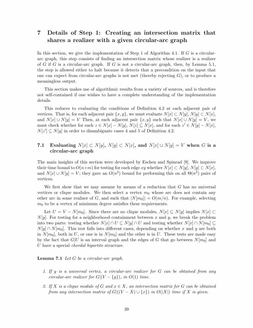
7 Details of Step 1: Creating an intersection matrix thatshares a realizer with a given circular-arc graph

In this section, we give the implementation of Step 1 of Algorithm 4.1. If G is a circular-arc graph, this step consists of finding an intersection matrix whose realizer is a realizerof G if G is a circular-arc graph. If G is not a circular-arc graph, then, by Lemma 5.1,the step is allowed either to halt because it detects that a precondition on the input thatone can expect from circular-arc graphs is not met (thereby rejecting G), or to produce ameaningless output.

This section makes use of algorithmic results from a variety of sources, and is thereforenot self-contained if one wishes to have a complete understanding of the implementationdetails.

This reduces to evaluating the conditions of Definition 4.2 at each adjacent pair ofvertices. That is, for each adjacent pair x, y, we must evaluate N [x] ⊂ N [y], N [y] ⊂ N [x],and N [x] ∪ N [y] = V Then, at each adjacent pair x, y such that N [x] ∪ N [y] = V , wemust check whether for each z ∈ N [x]−N [y], N [z] ⊆ N [x], and for each z′ ∈ N [y]−N [x],N [z′] ⊆ N [y] in order to disambiguate cases 4 and 5 of Definition 4.2.

7.1 Evaluating N [x] ⊂ N [y], N [y] ⊂ N [x], and N [x] ∪ N [y] = V when G is acircular-arc graph

The main insights of this section were developed by Eschen and Spinrad [9]. We improvetheir time bound to O(n+m) for testing for each edge xy whether N [x] ⊂ N [y], N [y] ⊂ N [x],and N [x] ∪N [y] = V ; they gave an O(n2) bound for performing this on all Θ(n2) pairs ofvertices.

We first show that we may assume by means of a reduction that G has no universalvertices or clique modules. We then select a vertex m0 whose arc does not contain anyother arc in some realizer of G, and such that |N [m0]| = O(m/n). For example, selectingm0 to be a vertex of minimum degree satisfies these requirements.

Let U = V − N [m0]. Since there are no clique modules, N [x] ⊆ N [y] implies N [x] ⊂N [y]. For testing for a neighborhood containment between x and y, we break the probleminto two parts: testing whether N [x] ∩ U ⊆ N [y] ∩ U and testing whether N [x] ∩N [m0] ⊆N [y] ∩N [m0]. This test falls into different cases, depending on whether x and y are bothin N [m0], both in U , or one is in N [m0] and the other is in U . These tests are made easyby the fact that G|U is an interval graph and the edges of G that go between N [m0] andU have a special chordal bipartite structure.

Lemma 7.1 Let G be a circular-arc graph.

1. If y is a universal vertex, a circular-arc realizer for G can be obtained from anycircular-arc realizer for G|(V − y), in O(1) time.

2. If X is a clique module of G and x ∈ X, an intersection matrix for G can be obtainedfrom any intersection matrix of G|((V −X) ∪ x) in O(|X|) time if X is given.

39

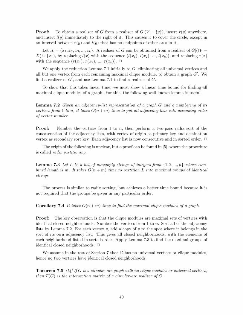
Proof: To obtain a realizer of G from a realizer of G|(V − y), insert r(y) anywhere,and insert l(y) immediately to the right of it. This causes it to cover the circle, except inan interval between r(y) and l(y) that has no endpoints of other arcs in it.

Let X = x1, x2, x3, ..., xk. A realizer of G can be obtained from a realizer of G|((V −X) ∪ x), by replacing l(x) with the sequence (l(x1), l(x2), ..., l(xk)), and replacing r(x)with the sequence (r(x1), r(x2), ..., r(xk)). 2

We apply the reduction Lemma 7.1 initially to G, eliminating all universal vertices andall but one vertex from each remaining maximal clique module, to obtain a graph G′. Wefind a realizer of G′, and use Lemma 7.1 to find a realizer of G.

To show that this takes linear time, we must show a linear time bound for finding allmaximal clique modules of a graph. For this, the following well-known lemma is useful.

Lemma 7.2 Given an adjacency-list representation of a graph G and a numbering of itsvertices from 1 to n, it takes O(n + m) time to put all adjacency lists into ascending orderof vertex number.

Proof: Number the vertices from 1 to n, then perform a two-pass radix sort of theconcatenation of the adjacency lists, with vertex of origin as primary key and destinationvertex as secondary sort key. Each adjacency list is now consecutive and in sorted order. 2

The origin of the following is unclear, but a proof can be found in [5], where the procedureis called radix partitioning.

Lemma 7.3 Let L be a list of nonempty strings of integers from 1, 2, ..., n whose com-bined length is m. It takes O(n + m) time to partition L into maximal groups of identicalstrings.

The process is similar to radix sorting, but achieves a better time bound because it isnot required that the groups be given in any particular order.

Corollary 7.4 It takes O(n + m) time to find the maximal clique modules of a graph.

Proof: The key observation is that the clique modules are maximal sets of vertices withidentical closed neighborhoods. Number the vertices from 1 to n. Sort all of the adjacencylists by Lemma 7.2. For each vertex v, add a copy of v to the spot where it belongs in thesort of its own adjacency list. This gives all closed neighborhoods, with the elements ofeach neighborhood listed in sorted order. Apply Lemma 7.3 to find the maximal groups ofidentical closed neighborhoods. 2

We assume in the rest of Section 7 that G has no universal vertices or clique modules,hence no two vertices have identical closed neighborhoods.

Theorem 7.5 [14] If G is a circular-arc graph with no clique modules or universal vertices,then T (G) is the intersection matrix of a circular-arc realizer of G.

40

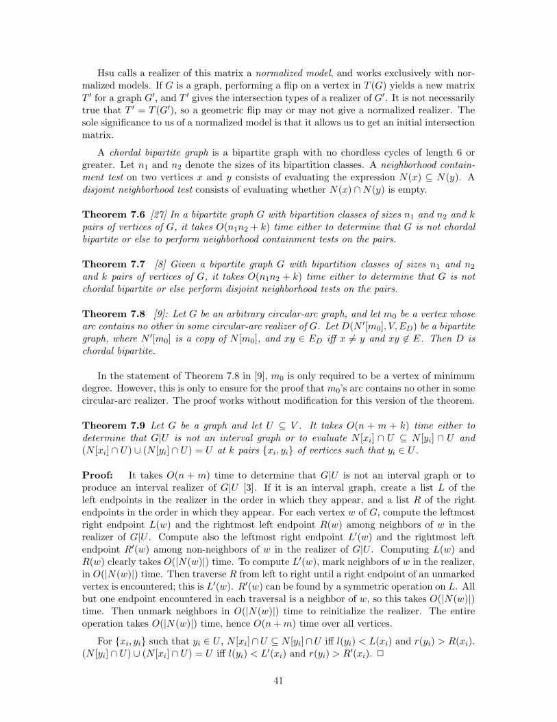
Hsu calls a realizer of this matrix a normalized model, and works exclusively with nor-malized models. If G is a graph, performing a flip on a vertex in T (G) yields a new matrixT ′ for a graph G′, and T ′ gives the intersection types of a realizer of G′. It is not necessarilytrue that T ′ = T (G′), so a geometric flip may or may not give a normalized realizer. Thesole significance to us of a normalized model is that it allows us to get an initial intersectionmatrix.

A chordal bipartite graph is a bipartite graph with no chordless cycles of length 6 orgreater. Let n1 and n2 denote the sizes of its bipartition classes. A neighborhood contain-ment test on two vertices x and y consists of evaluating the expression N(x) ⊆ N(y). Adisjoint neighborhood test consists of evaluating whether N(x) ∩N(y) is empty.

Theorem 7.6 [27] In a bipartite graph G with bipartition classes of sizes n1 and n2 and kpairs of vertices of G, it takes O(n1n2 + k) time either to determine that G is not chordalbipartite or else to perform neighborhood containment tests on the pairs.

Theorem 7.7 [8] Given a bipartite graph G with bipartition classes of sizes n1 and n2

and k pairs of vertices of G, it takes O(n1n2 + k) time either to determine that G is notchordal bipartite or else perform disjoint neighborhood tests on the pairs.

Theorem 7.8 [9]: Let G be an arbitrary circular-arc graph, and let m0 be a vertex whosearc contains no other in some circular-arc realizer of G. Let D(N ′[m0], V, ED) be a bipartitegraph, where N ′[m0] is a copy of N [m0], and xy ∈ ED iff x 6= y and xy 6∈ E. Then D ischordal bipartite.

In the statement of Theorem 7.8 in [9], m0 is only required to be a vertex of minimumdegree. However, this is only to ensure for the proof that m0’s arc contains no other in somecircular-arc realizer. The proof works without modification for this version of the theorem.

Theorem 7.9 Let G be a graph and let U ⊆ V . It takes O(n + m + k) time either todetermine that G|U is not an interval graph or to evaluate N [xi] ∩ U ⊆ N [yi] ∩ U and(N [xi] ∩ U) ∪ (N [yi] ∩ U) = U at k pairs xi, yi of vertices such that yi ∈ U .

Proof: It takes O(n + m) time to determine that G|U is not an interval graph or toproduce an interval realizer of G|U [3]. If it is an interval graph, create a list L of theleft endpoints in the realizer in the order in which they appear, and a list R of the rightendpoints in the order in which they appear. For each vertex w of G, compute the leftmostright endpoint L(w) and the rightmost left endpoint R(w) among neighbors of w in therealizer of G|U . Compute also the leftmost right endpoint L′(w) and the rightmost leftendpoint R′(w) among non-neighbors of w in the realizer of G|U . Computing L(w) andR(w) clearly takes O(|N(w)|) time. To compute L′(w), mark neighbors of w in the realizer,in O(|N(w)|) time. Then traverse R from left to right until a right endpoint of an unmarkedvertex is encountered; this is L′(w). R′(w) can be found by a symmetric operation on L. Allbut one endpoint encountered in each traversal is a neighbor of w, so this takes O(|N(w)|)time. Then unmark neighbors in O(|N(w)|) time to reinitialize the realizer. The entireoperation takes O(|N(w)|) time, hence O(n + m) time over all vertices.

For xi, yi such that yi ∈ U , N [xi]∩U ⊆ N [yi]∩U iff l(yi) < L(xi) and r(yi) > R(xi).(N [yi] ∩ U) ∪ (N [xi] ∩ U) = U iff l(yi) < L′(xi) and r(yi) > R′(xi). 2

41

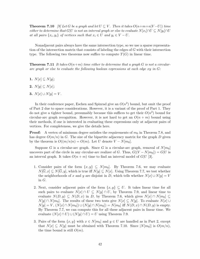
Theorem 7.10 [9] Let G be a graph and let U ⊆ V . Then it takes O(n+m+n|V −U |) timeeither to determine that G|U is not an interval graph or else to evaluate N [xi]∩U ⊆ N [yi]∩Uat all pairs xi, yi of vertices such that xi ∈ U and yi ∈ V − U .

Nonadjacent pairs always have the same intersection type, so we use a sparse representa-tion of the intersection matrix that consists of labeling the edges of G with their intersectiontype. The following two theorems now suffice to compute T (G) in linear time.

Theorem 7.11 It takes O(n+m) time either to determine that a graph G is not a circular-arc graph or else to evaluate the following boolean expressions at each edge xy in G:

1. N [x] ⊆ N [y];

2. N [y] ⊆ N [x];

3. N [x] ∪N [y] = V .

In their conference paper, Eschen and Spinrad give an O(n2) bound, but omit the proofof Part 2 due to space considerations. However, it is a variant of the proof of Part 1. Theydo not give a tighter bound, presumably because this suffices to get their O(n2) bound forcircular-arc graph recognition. However, it is not hard to get an O(n + m) bound usingtheir methods, if one is interested in evaluating these expressions only at adjacent pairs ofvertices. For completeness, we give the details here.

Proof: A vertex of minimum degree satisfies the requirements of m0 in Theorem 7.8, andhas degree O(m/n) in G. The size of the bipartite adjacency matrix for the graph D givenby the theorem is O((m/n)n) = O(m). Let U denote V −N [m0].

Suppose G is a circular-arc graph. Since G is a circular-arc graph, removal of N [m0]uncovers part of the circle in any circular-arc realizer of G. Thus, G|(V −N [m0]) = G|U isan interval graph. It takes O(n + m) time to find an interval model of G|U [3].

1. Consider pairs of the form x, y ⊆ N [m0]. By Theorem 7.6, we may evaluateN [G, x] ⊆ N [G, y], which is true iff N [y] ⊆ N [x]. Using Theorem 7.7, we test whetherthe neighborhoods of x and y are disjoint in D, which tells whether N [x] ∪N [y] = Vin G.

2. Next, consider adjacent pairs of the form x, y ⊆ U . It takes linear time for allsuch pairs to evaluate N [x] ∩ U ⊆ N [y] ∩ U , by Theorem 7.9, and linear time toevaluate N(D, y) ⊆ N(D,x) in D, by Theorem 7.6, which gives N [x] ∩ N [m0] ⊆N [y] ∩ N [m0]. The results of these two tests give N [x] ⊆ N [y]. To evaluate N [x] ∪N [y] = V , (N [x]∩N [m0])∪ (N [y]∩N [m0]) = N [m0] iff N(D,x)∩N(D, y) is empty.By Theorem 7.7, we can compute this for all these adjacent pairs in linear time. Weevaluate (N [x] ∩ U) ∪ (N [y] ∩ U) = U using Theorem 7.9.

3. Pairs of the form x, y with x ∈ N [m0] and y ∈ U are handled as in Part 2, exceptthat N [x] ⊆ N [y] must be obtained with Theorem 7.10. Since |N [m0]| is O(m/n),the time bound is still O(m).

42

Now, suppose that G is not a circular-arc graph. If Theorem 7.6, 7.7, 7.9, or 7.10 fail todeliver the required results, then this can only be because they determined that a subgraphfailed to satisfy a property that we have shown that it must satisfy if G is a circular-arcgraph. 2

By itself, Theorem 7.11 does not give circular-arc graph recognition, because it allowsfor the possibility that when G is not a circular-arc graph, G fails to be rejected, and insteadthe claimed tests are performed correctly.

7.2 Disambiguating Cases 4 and 5 of Definition 4.2

In this subsection, we show the following, which is all that remains to do in order todisambiguate Cases 4 and 5 of Definition 4.2:

Theorem 7.12 It takes O(n + m) time either to determine that G is not a circular-arcgraph or else to evaluate the following boolean expressions at each edge xy in G such thatN [x] ∪N [y] = V :

For each z ∈ N [x]−N [y], N [z] ⊆ N [x], and for each z′ ∈ N [y]−N [x], N [z′] ⊆ N [y].

An O(n2) bound for evaluating this in the special case where the vertices can be par-titioned into two cliques is given in [9]. We need a linear bound for arbitrary circular-arcgraphs.

The strategy of the proof can be summarized as follows. If N [x] ∪ N [y] = V , then wecan reduce the problem to one we have already solved, by flipping y in some realizer toobtain y′ and testing whether N [y′] ⊆ N [x] in the graph represented by the new realizer.We do not yet know a realizer of G, but Theorem 7.11 provides enough information to allowus to deduce the effect on G of flipping y.

However, to obtain the linear time bound, we must batch these tests together by addingto G a copy y′ of one vertex y out of every pair x, y such that N [x] ∪N [y] = V . Let Vbe the original vertices and F be the copies. We then flip all the copies to obtain a graphH with vertex set V ∪ F . We then perform the comparison on x and y by testing whetherN [y′] ∩ V ⊆ N [x] ∩ V in H.

This gives rise to an obstacle in applying the technique: If x′, y′ ∈ F , then we do notknow whether they are adjacent in H. This depends on whether xy falls into Case 4 or Case5. If xy is a single overlap, in G then x′y′ is a single overlap in H, which is an adjacency,but if xy is a double overlap, then x′y′ fails to be an edge in H. Thus, we do not knowH|F , and we must avoid use of its edges when applying our tests.

Let m0 be a vertex such whose arc contains no other in a circular-arc representation ofH. We use two key facts in order to employ techniques from the previous subsection:

1. H|(V −N [m0]) = G|(V −N [m0]) is an interval graph.

2. Let D be the bipartite graph D(N [m0], F ∪ V ), that is obtained as described byTheorem 7.8 applied to H. Then D is chordal bipartite, as is every induced subgraphof D.

43

We split the test into two parts: testing whether N [y′]∩(V ∩N [m0]) ⊆ N [x]∩(V ∩N [m0])and testing whether N [y′]∩ (V −N [m0]) ⊆ N [x]∩ (V −N [m0]). These tests are performedusing the two key facts and techniques similar to those of Section 7.1. How they are applieddepends on which of x and y′ are neighbors of m0.

Computing D requires knowledge of edges of H|F , which we do not have. We get aroundthis problem by instead making use of two induced subgraphs D1 and D2 of D, neither ofwhich requires information about H|F to compute, and which suffice to make the requiredtests of neighborhood containments. This trick resolves all of the cases, except the onewhere x is a neighbor of m0 in H and y′ is not. In this case, we must improvise a newtechnique, which is based on a type of graph called a probe interval graphs, which we definebelow.

A remaining issue is that, to apply our techniques, we must identify a vertex m0 ofH such that there is a circular-arc realizer of H where arc m0 contains no other arc,|N [m0]| = O(m/n), and m0 6∈ F . The requirement that m0 contain no other arc is necessaryto apply Eschen and Spinrad’s theorems. The requirement that |N [m0]| = O(m/n) isrequired for the time bound. That m0 6∈ F is required because we need to know N [m0],and if m0 ∈ F , this requires knowledge of H|F .

We first show how to find an m0 that satisfies all of the requirements with the possibleexception of m0 6∈ F . If m0 ∈ F , we modify H, V , and F slightly so that it still suits ourpurposes and m0 6∈ F .

This concludes the summary of the strategy. We now give the detailed proof.

A probe interval graph is a graph G = (V,E) and a partition P,N of V such thatG|P is an interval graph, N is an independent set, and there is an interval realizer on Vwhere edges of P × V can be realized with an interval model. There are no restrictionson adjacencies and nonadjacencies assigned by the realizer among members of N . Such arealizer of G is a probe interval realizer.

Theorem 7.13 [20] Given a graph G and a partition P,N of its vertices, it takesO(n + m + n|N |) time to construct a probe interval model or else determine that G is nota probe interval graph with respect to the partition P,N.

Johnson and Spinrad showed an O(n2) variant of Theorem 7.13 [15]. We have modifiedit to get an O(n+m log n) bound [21], and the proof of Theorem 7.13 differs from this proofone by allowing O(n) time, rather than O(log n) time, to incorporate each non-probe intothe model.

Theorem 7.14 Let G be a graph, and let U ⊆ V , and a partition P,N of U . It takesO(n + m + n|V − P |) time either to determine that G|U is not a probe interval graph withrespect to the partition P,N, or else evaluate N [x] ∩ P ⊆ N [y] ∩ P at all adjacent pairsx, y such that at most one of x and y is in V − U .

Proof: If G|U is not a probe interval graph with respect to P,N, then we may detectthis in linear time, by Theorem 7.13. Otherwise, we obtain a probe interval model R thatrealizes G|U . The algorithms of Theorems 7.9 and 7.10 can be trivially adapted to theproblem. For Theorem 7.9, compute L(w), R(w), L′(w) and R′(w) in R|P , and let l(y) and

44

r(y) denote the position of y ∈ U relative endpoints of P . The test is now identical. Anidentical adaptation suffices for the algorithm of Theorem 7.10 given in [9]. 2

Algorithm 7.15 Build an auxilliary graph for Theorem 7.12.

• Compute neighborhood containments in G and pairs of the form xy ∈ G(T ) andN [x] ∪N [y] = V , using Theorem 7.11.

• For each xy ∈ G(T ) such that N [x] ∪N [y] = V :

– Find one of the two vertices, say, x, with degree at least as large as the other.

– Insert a copy x′ into G if one has not already been inserted, and make it adjacentto x, thereby making x, x′ a clique module.

• Let us call this graph H ′, and the set of new vertices F .

At this point, let us pause to define some objects that we do not compute explicitly,but that we can now compute limited information about. Let R′ any the realizer ofH ′ derived from a realizer of T (G) by letting each added arc x′ ∈ F properly containits copy x in V . That is x and x′ have identical arcs in R′, except that the arccorresponding to x′ has been stretched slightly so that it properly contains that of x.(We do this to avoid the complications of realizers where endpoints of arcs coincide.)Let H be the circular-arc graph that results from flipping each x′ ∈ F in R′.

• Find a vertex m0 that minimizes |N [H,m0] ∩ V |.

• Return m0, H|V , and the edges of H that go between V and F .

Lemma 7.16 Algorithm 7.15 takes O(n + m) time and |F | = O(m/n).

Proof: The size of H ′ is O(n + m). Since there are O(m) edges in H ′, the sum ofdegrees of members of F in H ′ is O(m) in H ′. Each vertex in F has degree Ω(n) in H ′,so |F | = O(m/n). We may spend O(n) time on each member of F without exceedingO(n + m). Since each member of F has Ω(n) incident edges in H ′ and O(n) incident edgesin H, the size of H is also O(n + m).

The critical observation is that the algorithm does not need to compute edges in H|Fin order to be able to return the result. H|V = G, so these edges are already available. Forx ∈ V and y′ ∈ F , let y be the unflipped copy of y′ in V . Since G has no clique modules,xy′ fails to be an edge of H iff N [G, x] ⊂ N [G, y]. N [G, x] ⊂ N [G, y] only if x and y areadjacent in G, so the results of this test are known from the first step of the algorithm.Since |F | is O(m/n), the time bound follows for these pairs. 2

Lemma 7.17 Let m0 be a vertex of H that minimizes |N [H,x]∩V |. If m0 ∈ V , then thereis a realizer R of H such that arc m0 contains no other.

Proof: Recall that G has no clique modules or universal vertices. Let RG be theunknown realizer of T (G) given by Theorem 7.5. Let R′ be the realizer of H ′ obtained fromRG by adding a copy y′ of each arc y of R that has a duplicate element of F in H ′. To

45

disambiguate what happens to the relationship of y and y′ when y′ is flipped, let us assumethat the endpoints of y′ have been stretched slightly so that y′ properly contains y. In thecircular ordering of endpoints in R′, the endpoints of y and y′ form two consecutive pairs.Let RH be the realizer of H obtained by flipping the members of F .

Let z′ be an arc such that N [H, z′]∩V = N [H,m0]∩V . Since m0 minimizes N [H,x]∩V ,only arcs of this form could be be contained in arc m0 in RH . Thus, if z′ does not exist, theclaim holds. Otherwise, if z′ ∈ V , then m0 and z′ are a clique module of G, a contradiction.Thus, z′ is the flipped copy of some z ∈ V . Because of the way the copy of z′ is created,z and z′ are nonadjacent, hence so are m0 and z. The endpoints of z and z′ make twoadjacent pairs in the circular ordering of endpoints in RH , so if arc z′ fails to contain arcm0 in RH , z is a neighbor of m0 in G, a contradiction. 2

In what follows, we let N [H,x] denote the neighborhood in H of x ∈ V ∪ F in H, andN [x] denote the neighborhood in G of x ∈ V .

Let m0 be the vertex returned by Algorithm 7.15. We need for m0 to be a member ofV . Let D be the chordal bipartite graph on H given by Theorem 7.8. Let D1(X ∪ Y, V )denote the subgraph induced by V and the copies of X ∪ Y in D, and let D2(X, V ∪ F ) bethe subgraph induced by the copies of V ∪ F and the copies of X. Neither of these graphsrequires knowledge of H|F to compute. They are both chordal bipartite because they areinduced subgraphs of D.

If m0 ∈ F , m0 is the twin of some x ∈ V , and each y′ ∈ F is the twin of some y ∈ V .If x and y are adjacent and N [x] ∪ N [y] = V , then we do not know whether m0 andy′ are adjacent, since we do not know whether x and y have a single or double overlap.However, since we already know neighborhood containments among adjacent pairs in V wecan find out in O(n) time for all z ∈ N [x] − N [y], whether N [z] ⊆ N [x]. Similarly, wecan find for all z′ ∈ N [y] − N [x] whether N [z] ⊂ N [y]. (As we see below, however, thissecond test is unnecessary.) Since |F | = O(m/n), all of these evaluations take O(m) time.This disambiguates Cases 4 and 5 on edges incident to x in G, which gives all edges ofH|(V ∪ m0) and all edges of H between m0 and members of F − m0. At this point,we reset G = H|(V ∪m0), V = V ∪ m0, F = F − m0. We remove universal verticesand collapse clique modules as before. We rerun Algorithm 7.15, but this time, there is noneed to insert a copy of m0 and flip it, since G already has one. We select the same m0 toreturn as the first time. It is still true that |N [H,m0] ∩ V | is minimized. Now, m0 ∈ V ,and Algorithm 7.15 gives us H|V and edges of H from V to F . By Lemma 7.17, m0’s arccontains no other arc in some realizer of H.

For each pair x, y such that N [x] ∪N [y] = V , at least one of x and y has a copy in F .Suppose without loss of generality that y has a copy y′ in F . Suppose N [x] ∪N [y] = V . Iffor some z ∈ N [x] − N [y], N [z] 6⊂ N [x], then z has a neighbor that x does not have, andthis neighbor must be a neighbor z′ of y that x does not have. Since N [x] ∪ N [y] = V ,this implies that z′ ∈ N [y] − N [x], and N [z′] 6⊂ N [y], since z′ has a neighbor, z, thaty does not have. Testing for all z ∈ N [x] − N [y] whether N [z] ⊂ N [x] suffices for theseemingly stronger requirement of the fourth condition in the definition of T (G), where thecondition on z′ is redundant. But the non-neighbors neighbors of y in V are exactly theneighbors of y′ in V whose neighborhoods in V are contained in y′. The condition is trueiff N [H, y′] ∩ V ⊆ N [H,x] ∩ V .

46

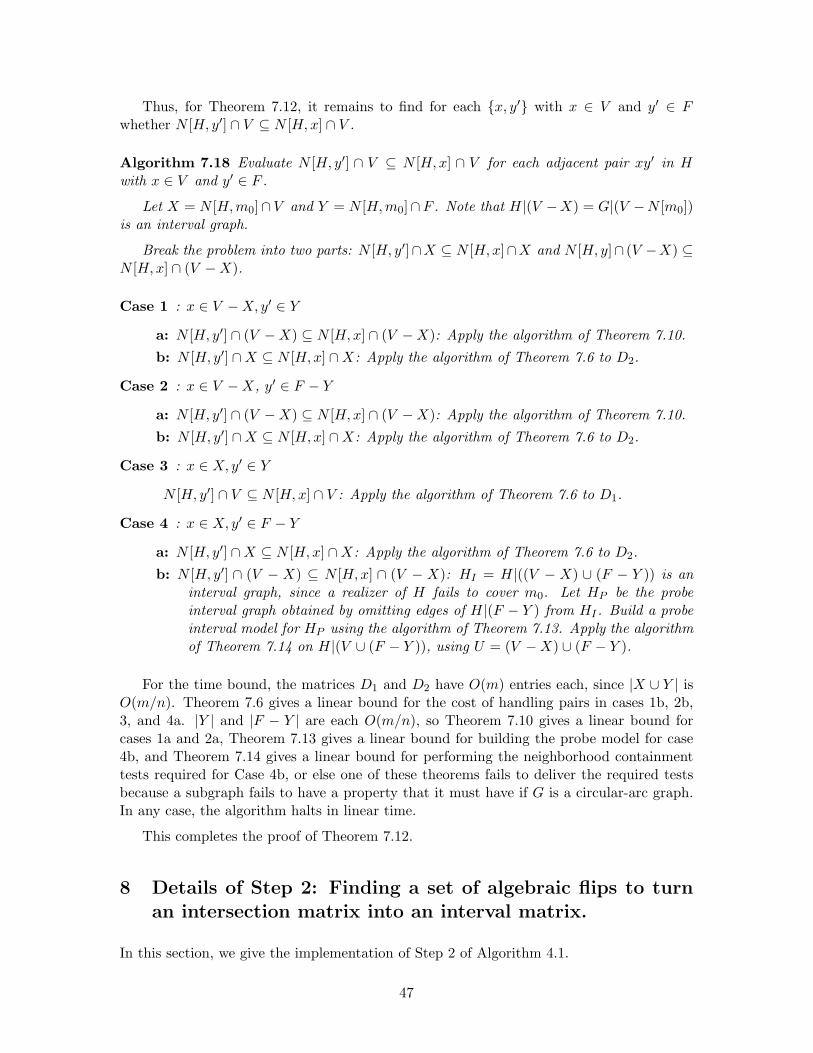
Thus, for Theorem 7.12, it remains to find for each x, y′ with x ∈ V and y′ ∈ Fwhether N [H, y′] ∩ V ⊆ N [H,x] ∩ V .

Algorithm 7.18 Evaluate N [H, y′] ∩ V ⊆ N [H,x] ∩ V for each adjacent pair xy′ in Hwith x ∈ V and y′ ∈ F .

Let X = N [H,m0]∩V and Y = N [H,m0]∩F . Note that H|(V −X) = G|(V −N [m0])is an interval graph.

Break the problem into two parts: N [H, y′]∩X ⊆ N [H,x]∩X and N [H, y]∩ (V −X) ⊆N [H,x] ∩ (V −X).

Case 1 : x ∈ V −X, y′ ∈ Y

a: N [H, y′] ∩ (V −X) ⊆ N [H,x] ∩ (V −X): Apply the algorithm of Theorem 7.10.

b: N [H, y′] ∩X ⊆ N [H,x] ∩X: Apply the algorithm of Theorem 7.6 to D2.

Case 2 : x ∈ V −X, y′ ∈ F − Y

a: N [H, y′] ∩ (V −X) ⊆ N [H,x] ∩ (V −X): Apply the algorithm of Theorem 7.10.

b: N [H, y′] ∩X ⊆ N [H,x] ∩X: Apply the algorithm of Theorem 7.6 to D2.

Case 3 : x ∈ X, y′ ∈ Y

N [H, y′] ∩ V ⊆ N [H,x] ∩ V : Apply the algorithm of Theorem 7.6 to D1.

Case 4 : x ∈ X, y′ ∈ F − Y

a: N [H, y′] ∩X ⊆ N [H,x] ∩X: Apply the algorithm of Theorem 7.6 to D2.

b: N [H, y′] ∩ (V − X) ⊆ N [H,x] ∩ (V − X): HI = H|((V − X) ∪ (F − Y )) is aninterval graph, since a realizer of H fails to cover m0. Let HP be the probeinterval graph obtained by omitting edges of H|(F − Y ) from HI . Build a probeinterval model for HP using the algorithm of Theorem 7.13. Apply the algorithmof Theorem 7.14 on H|(V ∪ (F − Y )), using U = (V −X) ∪ (F − Y ).

For the time bound, the matrices D1 and D2 have O(m) entries each, since |X ∪ Y | isO(m/n). Theorem 7.6 gives a linear bound for the cost of handling pairs in cases 1b, 2b,3, and 4a. |Y | and |F − Y | are each O(m/n), so Theorem 7.10 gives a linear bound forcases 1a and 2a, Theorem 7.13 gives a linear bound for building the probe model for case4b, and Theorem 7.14 gives a linear bound for performing the neighborhood containmenttests required for Case 4b, or else one of these theorems fails to deliver the required testsbecause a subgraph fails to have a property that it must have if G is a circular-arc graph.In any case, the algorithm halts in linear time.

This completes the proof of Theorem 7.12.

8 Details of Step 2: Finding a set of algebraic flips to turnan intersection matrix into an interval matrix.

In this section, we give the implementation of Step 2 of Algorithm 4.1.

47

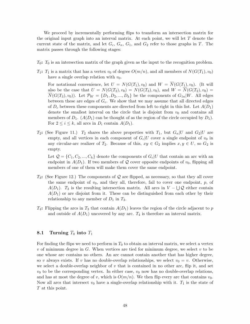
We proceed by incrementally performing flips to transform an intersection matrix forthe original input graph into an interval matrix. At each point, we will let T denote thecurrent state of the matrix, and let Gc, Gn, G1, and G2 refer to those graphs in T . Thematrix passes through the following stages:

T0: T0 is an intersection matrix of the graph given as the input to the recognition problem.

T1: T1 is a matrix that has a vertex v0 of degree O(m/n), and all members of N(G(T1), v0)have a single overlap relation with v0.

For notational convenience, let U = N(G(T1), v0) and W = N(G(T1), v0). (It willalso be the case that U = N(G(T2), v0) = N(G(T3), v0), and W = N(G(T2), v0) =N(G(T3), v0)). Let PW = D1, D2, ..., Dk be the components of G1n|W . All edgesbetween these are edges of Gc. We show that we may assume that all directed edgesof Dc between these components are directed from left to right in this list. Let A(D1)denote the smallest interval on the circle that is disjoint from v0 and contains allmembers of D1. (A(D1) can be thought of as the region of the circle occupied by D1).For 2 ≤ i ≤ k, all arcs in Di contain A(D1).

T2: (See Figure 11.) T2 shares the above properties with T1, but Gn|U and G2|U areempty, and all vertices in each component of Gc|U cover a single endpoint of v0 inany circular-arc realizer of T2. Because of this, xy ∈ G2 implies x, y ∈ U , so G2 isempty.

Let Q = C1, C2, ..., Ch denote the components of Gc|U that contain an arc with anendpoint in A(D1). If two members of Q cover opposite endpoints of v0, flipping allmembers of one of them will make them cover the same endpoint.

T3: (See Figure 12.) The components of Q are flipped, as necessary, so that they all coverthe same endpoint of v0, and they all, therefore, fail to cover one endpoint, p, ofA(D1). T3 is the resulting intersection matrix. All arcs in V −

⋃Q either contain

A(D1) or are disjoint from it. These can be distinguished from each other by theirrelationship to any member of D1 in T3.

T4: Flipping the arcs in T3 that contain A(D1) leaves the region of the circle adjacent to pand outside of A(D1) uncovered by any arc. T4 is therefore an interval matrix.

8.1 Turning T0 into T1

For finding the flips we need to perform in T0 to obtain an interval matrix, we select a vertexv of minimum degree in G. When vertices are tied for minimum degree, we select v to beone whose arc contains no others. An arc cannot contain another that has higher degree,so v always exists. If v has no double-overlap relationships, we select v0 = v. Otherwise,we select a double-overlap neighbor of v that is contained in no other arc, flip it, and setv0 to be the corresponding vertex. In either case, v0 now has no double-overlap relations,and has at most the degree of v, which is O(m/n). We then flip every arc that contains v0.Now all arcs that intersect v0 have a single-overlap relationship with it. T1 is the state ofT at this point.

48

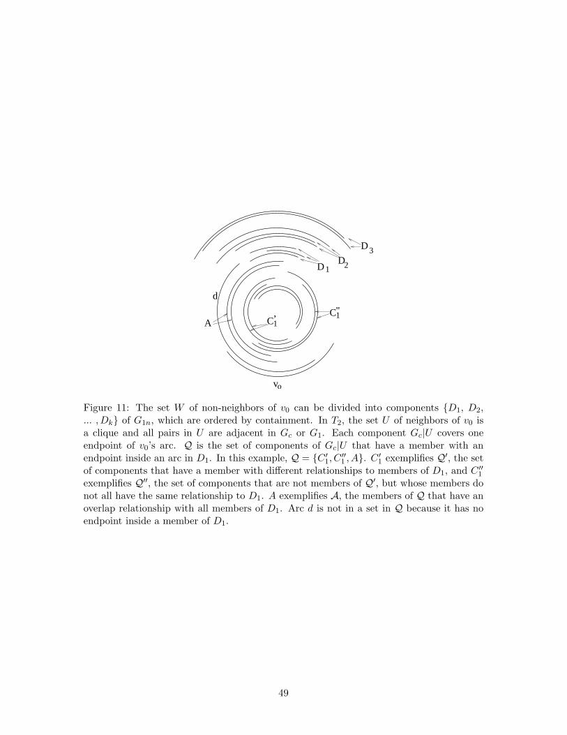
vo

D3D2D1

C1C1A

"’

d

Figure 11: The set W of non-neighbors of v0 can be divided into components D1, D2,... , Dk of G1n, which are ordered by containment. In T2, the set U of neighbors of v0 isa clique and all pairs in U are adjacent in Gc or G1. Each component Gc|U covers oneendpoint of v0’s arc. Q is the set of components of Gc|U that have a member with anendpoint inside an arc in D1. In this example, Q = C ′

1, C′′1 , A. C ′

1 exemplifies Q′, the setof components that have a member with different relationships to members of D1, and C ′′

1

exemplifies Q′′, the set of components that are not members of Q′, but whose members donot all have the same relationship to D1. A exemplifies A, the members of Q that have anoverlap relationship with all members of D1. Arc d is not in a set in Q because it has noendpoint inside a member of D1.

49

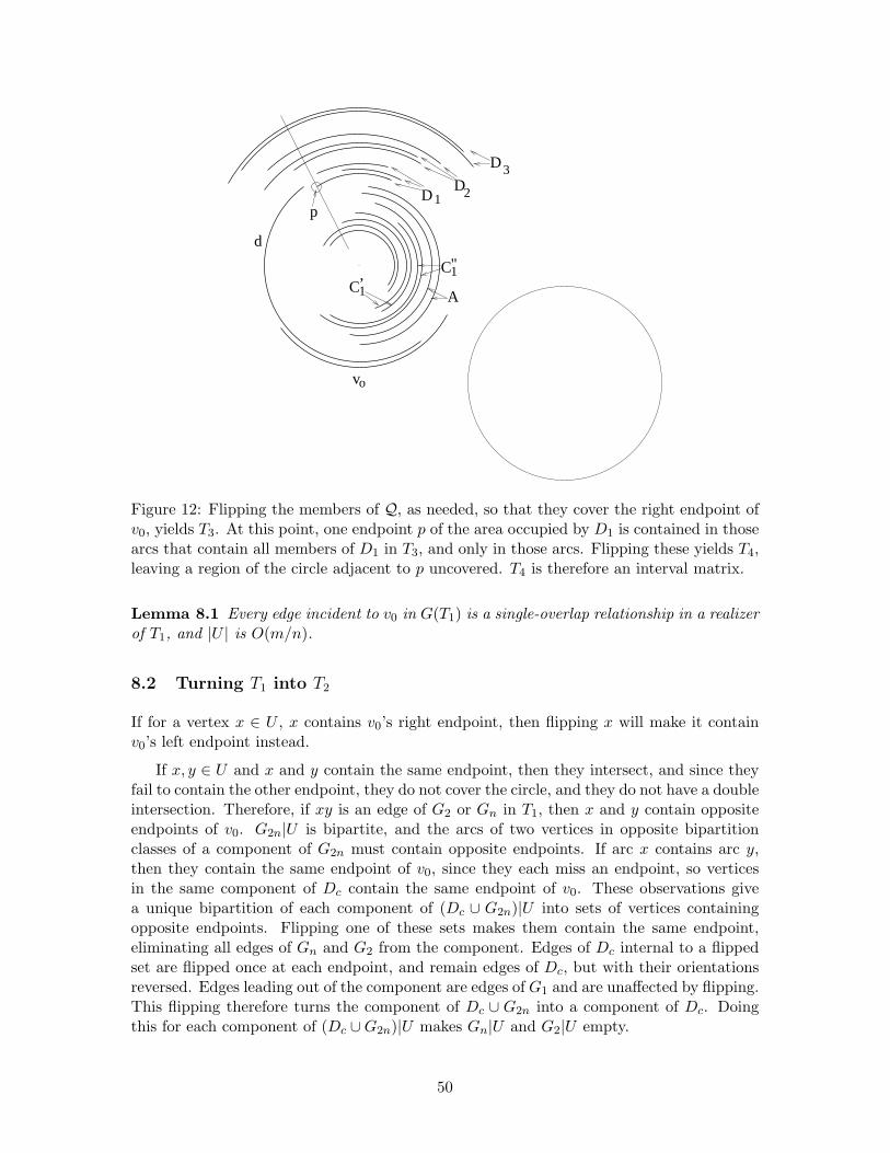
vo

D3D2D1

C1C1’

"

A

d

p

Figure 12: Flipping the members of Q, as needed, so that they cover the right endpoint ofv0, yields T3. At this point, one endpoint p of the area occupied by D1 is contained in thosearcs that contain all members of D1 in T3, and only in those arcs. Flipping these yields T4,leaving a region of the circle adjacent to p uncovered. T4 is therefore an interval matrix.

Lemma 8.1 Every edge incident to v0 in G(T1) is a single-overlap relationship in a realizerof T1, and |U | is O(m/n).

8.2 Turning T1 into T2

If for a vertex x ∈ U , x contains v0’s right endpoint, then flipping x will make it containv0’s left endpoint instead.

If x, y ∈ U and x and y contain the same endpoint, then they intersect, and since theyfail to contain the other endpoint, they do not cover the circle, and they do not have a doubleintersection. Therefore, if xy is an edge of G2 or Gn in T1, then x and y contain oppositeendpoints of v0. G2n|U is bipartite, and the arcs of two vertices in opposite bipartitionclasses of a component of G2n must contain opposite endpoints. If arc x contains arc y,then they contain the same endpoint of v0, since they each miss an endpoint, so verticesin the same component of Dc contain the same endpoint of v0. These observations givea unique bipartition of each component of (Dc ∪ G2n)|U into sets of vertices containingopposite endpoints. Flipping one of these sets makes them contain the same endpoint,eliminating all edges of Gn and G2 from the component. Edges of Dc internal to a flippedset are flipped once at each endpoint, and remain edges of Dc, but with their orientationsreversed. Edges leading out of the component are edges of G1 and are unaffected by flipping.This flipping therefore turns the component of Dc ∪ G2n into a component of Dc. Doingthis for each component of (Dc ∪G2n)|U makes Gn|U and G2|U empty.

50

Lemma 8.2 Lemma 8.1 applies to T2. In addition, all arcs in each of the components ofGc|U contain the same endpoint of v0 in any realizer of T2.

8.3 Turning T2 into T3

(See Figure 11.) Let Q′ = C ′1, C

′2, ..., C

′h′ be the components of Dc|U that have a member

that distinguishes members of D1, and let Q′′ = C ′′1 , C ′′

2 , ..., C ′′h′′ be the set C : C is a

component of Dc|U , C 6∈ Q′ and there is a member of D1 that distinguishes members ofC. Let A denote the set set A : A is a component of Gc|U such that A × D1 ⊆ G1.Q = Q′ ∪Q′′ ∪ A.

We obtain T3 from T2 as follows:

Case A: If Q′′ is nonempty, we use a single rule to decide which members of Q = Q′′ ∪Q′

to flip to get them all to cover a single endpoint of v0;

Case B: If Q′′ is empty, we use a different rule to decide which members of Q′ to flip toget them all to cover a single endpoint of v0;

Let T ′3 denote the resulting matrix. We show that there is a realizer of T ′

3 where allmembers of A also cover this same endpoint, so T3 = T ′

3.

8.3.1 Case A: Q′′ is nonempty

Let us say that if xz ∈ Gn and yz ∈ G1, then y has a stronger relationship to z than x does,since y and z intersect, but x and z do not. If xz ∈ G1 and yz ∈ Gc, then y again has astronger relationship with z than x does, since it is a full containment, rather than a partialoverlap. Similarly, if xz ∈ Gn and yz ∈ Gc, then the relationship of y to z is stronger thanthe relationship of x to z.

For x, y ∈ U , let x y denote that for every z ∈ W , the relationship of y to z is at leastas strong as the relationship of x to z. That is, x y if N(G1c, x)∩W ⊆ N(G1c, y)∩W andN(Gc, x) ∩W ⊆ N(Gc, y) ∩W . If A and B are two components of Gc|U , then let A Bdenote that for every x ∈ A and y ∈ B, x y. Let A ∼ B denote that A B or B A.

Lemma 8.3 If A and B are components of Gc|U and cover the same endpoint of v0 in acircular-arc realizer of T2, then A ∼ B.

Proof: Suppose A and B both cover the right endpoint of v0 in some circular-arc realizerR. Let A(W ) denote the smallest interval of the circle that is disjoint from v0 and containsevery arc in W . (Think of A(W ) as the “region occupied by W”.) Then for x ∈ A andy ∈ B, x and y both extend counterclockwise into A(W ). If A B and B A, the lemmaholds. Suppose without loss of generality that y extends farther than x does, so that y 6 x.Then every arc in W that is contained in x is also contained in y, and every arc in Wintersected by x is also intersected by y. Therefore, x y.

Since A and B contain no arc that covers the left endpoint of v0, R′ = R|(v0∪A∪B)is an interval realizer of T ′ = T |(v0 ∪ A ∪ B). The order of right endpoints in this

51

realizer is a linear extension of an interval orientation of T ′. The root node of the modulardecomposition of T ′ is a degenerate node whose children, v0, A, and B, are componentsin the complement of G1. G1n is transitively oriented in the interval orientation, so alledges of G1 between A and B must either be directed from A to B, or from B to A byLemma 6.1. Since x y and y 6 x, xy is oriented from x to y. Each arc of B extends atleast as far to the right as every arc of A, hence at least as far into the region occupied byW in R. It follows that A B. 2

G2 is empty, Dc is transitive, and D1, D2, ..., Dk are the children of the root of themodular decomposition of Gc|W . By Lemma 6.1, we may assume without loss of generalitythat Di ×Dj consists exclusively of arcs of Dc whenever 1 ≤ i < j ≤ k.

Lemma 8.4 If A ∈ Q′′, B ∈ Q′′ ∪Q′ and A 6= B, then A ∼ B iff A and B cover the sameendpoint of v0 in B.

Proof: Since A ∈ Q′′, A contains two vertices u and w that each have uniform relationshipsto all members of D1, but such that u’s relationship to D1 is different from w’s.

Case 1: u×D1 ⊆ Gn and w×D1 ⊆ Gc. Flipping A results in u×D1 ⊆ Gc andw ×D1 ⊆ Gn. In one of these cases, A and B cover the same endpoint of v0, so A ∼ B inone of these cases, by Lemma 8.3. In this case, either every member of B × D1 ⊆ Gc orevery member of B ×D1 ⊆ Gn, but this contradicts membership of B in Q. We concludethat Case 1 cannot occur.

Case 2: u ×D1 ⊆ G1 and w ×D1 ⊆ Gc. Suppose that we flip B as necessary sothat it covers the same endpoint as A does. If A B now applies, then B × D1 ⊆ Gc,contradicting B’s membership in Q. By Lemma 8.3, B A, so no member of B×D1 ∈ Gc.By B’s membership in Q′∪Q′′, there are pairs (a, b), (c, d) ∈ B×D1 such that ab ∈ Gn andcd ∈ G1 (where it is possible that a = c or b = d). Flipping B so that it does not containthe same endpoint of v0 as A results in ab ∈ Gc, and cd ∈ G1, and B 6∼ A. We concludethat the claim applies in Case 2.

Case 3: u ×D1 ⊆ G1 and w ×D1 ⊆ Gn. The proof is identical to that of Case 2,except that the roles of Gc and Gn are swapped. 2

Since every circular-arc realizer has a left-right mirror image, we may assume withoutloss of generality that C ′′

1 covers the right endpoint of v0 in R. Lemma 8.4 gives a simplecriterion for flipping the remaining members of Q′∪Q′′ so that they cover the same endpointof v0.

8.3.2 Case B: Q′′ is empty

If Q′′ is empty, then by mirror symmetry, we can assume without loss of generality that C ′1

covers the right endpoint of v0.

Our strategy is the following (See Figure 13). We find a vertex c1 ∈ C ′1 that distinguishes

members of D1. Suppose that c1 covers the right endpoint of v0 in some circular-arc realizerR. Since c1 is the only vertex in c1 ∪ D1 that intersects v0, c1 is a source (extremeleftmost interval) in the corresponding interval realizer R|(c1 ∪ D1). We use this and∆ relationships involving edges incident to c1 to find the interval realizer R|Pi for some

52

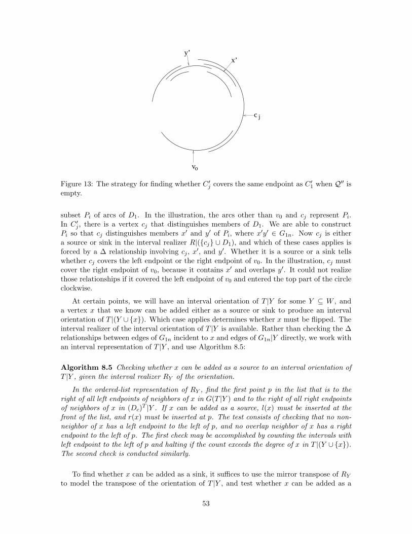
vo

c j

y’x’

Figure 13: The strategy for finding whether C ′j covers the same endpoint as C ′

1 when Q′′ isempty.

subset Pi of arcs of D1. In the illustration, the arcs other than v0 and cj represent Pi.In C ′

j , there is a vertex cj that distinguishes members of D1. We are able to constructPi so that cj distinguishes members x′ and y′ of Pi, where x′y′ ∈ G1n. Now cj is eithera source or sink in the interval realizer R|(cj ∪D1), and which of these cases applies isforced by a ∆ relationship involving cj , x′, and y′. Whether it is a source or a sink tellswhether cj covers the left endpoint or the right endpoint of v0. In the illustration, cj mustcover the right endpoint of v0, because it contains x′ and overlaps y′. It could not realizethose relationships if it covered the left endpoint of v0 and entered the top part of the circleclockwise.

At certain points, we will have an interval orientation of T |Y for some Y ⊆ W , anda vertex x that we know can be added either as a source or sink to produce an intervalorientation of T |(Y ∪x). Which case applies determines whether x must be flipped. Theinterval realizer of the interval orientation of T |Y is available. Rather than checking the ∆relationships between edges of G1n incident to x and edges of G1n|Y directly, we work withan interval representation of T |Y , and use Algorithm 8.5:

Algorithm 8.5 Checking whether x can be added as a source to an interval orientation ofT |Y , given the interval realizer RY of the orientation.

In the ordered-list representation of RY , find the first point p in the list that is to theright of all left endpoints of neighbors of x in G(T |Y ) and to the right of all right endpointsof neighbors of x in (Dc)T |Y . If x can be added as a source, l(x) must be inserted at thefront of the list, and r(x) must be inserted at p. The test consists of checking that no non-neighbor of x has a left endpoint to the left of p, and no overlap neighbor of x has a rightendpoint to the left of p. The first check may be accomplished by counting the intervals withleft endpoint to the left of p and halting if the count exceeds the degree of x in T |(Y ∪ x).The second check is conducted similarly.

To find whether x can be added as a sink, it suffices to use the mirror transpose of RY

to model the transpose of the orientation of T |Y , and test whether x can be added as a

53

source to it. The running time of Algorithm 8.5 is O(|N(G(T ), x))|).

Let R be a circular-arc realizer of T2. Let c1 be a member of C ′1 that distinguishes

members of D1, let cj be a member of C ′j that distinguishes members of D1, let P be v0

and the maximal modules of T2|(v0, c1∪D1) that do not contain v0, and let P be any setconsisting of one representative from each member of P. Let P ′ = P − v0, c1, andlet P ′ = P − v0, c1.

We may find R|P ′ as follows. T2|(v0, c1 ∪ D1) is an interval matrix with intervalrealizer R|(v0, c1 ∪ D1). In R|(v0, c1 ∪ D1), v0 is the interval with the leftmost leftendpoint, hence a source in the corresponding interval orientation of T2|(v0, c1 ∪ D1).Let us call Partition (Algorithm 6.22) on the initial partition v0, c1 ∪ D1 inT2 |(v0, c1 ∪D1), halting when each part is a module. The final partition is P, andby Lemma 6.24, Part 1, the ordering of its parts gives the unique interval orientation of(T2|(v0, c1 ∪ D1))/P that is consistent with v0 being a source. By Lemma 6.2, thecorresponding interval realizer R1 is unique. This quotient is isomorphic to T2|P , which isrealized by R|P . In R|P , v0 is also leftmost, so R|P is isomorphic to R1. By restriction,this gives R|P ′.

If there exists Z ∈ P ′ whose members have differing relationships to cj , let x1, x2 ∈ Z betwo vertices whose relationships to cj differ. Let P1 be x1 and one arbitrary representativeof each member of P ′ −Z, and let P2 be the result of replacing x1 in P1 with x2. One ofthese will serve as Pi. If Z does not exist, let P1 = P2 consist of one representative of eachmember of P ′. The algorithm for finding R|P works identically on R|P1 and R|P2, so R|P1

and R|P2 are isomorphic to R|P ′, and we do not have to recompute these interval realizersfor each C ′

j . The relationships of cj R|P1 and R|P2 may differ, however.

Lemma 8.6 cj can be added as a source to both R|P1 and R|P2 iff C ′1 and C ′

j cover thesame endpoint of v0.

Proof: Case 1: Z does not exist. Since cj distinguishes members of D1, it distinguishesX ∈ P ′ from Y ∈ P ′. Since G1n|D1 is connected, there exist X ′, Y ′ ∈ P ′ such thatX ′ × Y ′ ⊆ G1n. Let x′ and y′ be the representatives of X ′ and Y ′ in P1. Without loss ofgenerality, suppose x′ precedes y′ in R|P1.

If cj covers the same endpoint as c1 in R, then cj has the leftmost left endpoint in theinterval realizer R|(cj∪P1), so cj can be added as a source to R|P1, and the relationshipof cj to x′ is stronger than its relationship to y′. If cj is flipped so that it covers the oppositeendpoint of v0 from c1, R|(cj ∪ P1) is still an interval realizer, but with cj rightmost. Itsrelationship to x′ becomes weaker than its relationship to y′. Since x′ is earlier than y′ inR|(cj ∪ P1), cj can no longer be added as a source to R|P1.

Case 2: Z exists. Then cj distinguishes x1, x2 ∈ Z. Since D1 is connected and P ′

consists of modules of T2|(v0, c1 ∪D1), there exists Z ′ in P ′ such that Z ×Z ′ ⊆ G1n. Forany y in Z ′, either cj has different relationships to x1 and y or to x2 and y. Without loss ofgenerality, suppose it has different relationships to x1 and y. Now x1 and y have the sameproperties as x′ and y′ from Case 1, so cj can be added as a source to R|P1 iff cj and c1

cover the same endpoint of v0.

The results now follows from Lemma 8.2. 2

Lemma 8.6 and Algorithm 8.5 provide an efficient test for deciding how to flip members

54

of Q′ − C ′1 so that they cover the same endpoint of v0 as C ′

1 does, namely, the rightendpoint of v0.

8.3.3 Showing that T ′3 serves as T3

In T ′3, all arcs in members of Q′ and Q′′ cover the right endpoint of v0 in some realizer Rc

of T ′3. With the exception of arcs in A, this is all arcs that have an endpoint in A(D1).

Lemma 8.7 There is a circular-arc realizer of T ′3 where all members of Q′, Q′′, and A

cover the right endpoint of v0.

Proof: Let A be a member of A that covers the left endpoint of v0 in T ′3. By the definition

of A, A×D1 ⊆ G1. Therefore, A×Di ⊆ G1 for any i > 1, since Di ×D1 ⊆ (Dc)T , and D1

lies in the intersection of all arcs in Di, which are, in turn, disjoint from both endpoints ofv0. Members of A are connected components of G1n. The edges of G1 are unaffected byflipping, so flipping the members of A modifies T ′

3|A without affecting other relationshipsin T ′

3.

Since they are components of G1n, the members of A are children of the root of MD(T ).By Lemma 6.18, for each A ∈ A, the left endpoints of A are consecutive and the rightendpoints of A are consecutive.

If the members of A cover the left endpoint of v0, the only effect on the intersectionmatrix of flipping the members of A on the intersection matrix for the realizer is to reversethe directions of directed edges corresponding to Dc|A. This effect can then be undonewithout other side effects, by reversing the order of left endpoints of A and the order ofright endpoints of A within their respective segments of the circle. The net effect is tomove only those arcs that belong to A so that they cover the right endpoint of v0, withoutchanging the intersection matrix for the realizer.

Doing this to each A ∈ A that covers the left endpoint of v0 produces a realizer of T ′3

that satisfies the claim in the lemma. 2

Lemma 8.7 justifies letting T3 = T ′3. The following is now immediate:

Lemma 8.8 There exists a circular-arc realizer of T3 where every member of U with anendpoint inside the region of the circle occupied by D1 covers the right endpoint of v0.

8.4 Turning T3 into T4

The following corollary to Lemma 8.8 is now obvious:

Corollary 8.9 In such a realizer, let p be the far endpoint of the interval A(D1) as onetravels counterclockwise from the right endpoint of v0. An arc contains p in its interior iffit is one of the following:

• A member of D2, ..., Dk

55

• A member x of U such that x×D1 ⊆ Dc.

We may obtain T4 from T3 by flipping all arcs that contain p according to this corollary.This vacates the circle just to the right of p, so T4 is an interval matrix.

8.5 Linear-time implementation

For the analysis of the time bound, we must not assume that the input graph is a circular-arcgraph.

Theorems 7.11 and 7.12 ensure that we do not spend more than linear time findingneighborhood containments, even if G is not a circular-arc graph.

We use a labeling of edges of G(T ) with their intersection types for a sparse represen-tation of T . We may use an array to represent all intersection types in U × V . Since U hasO(m/n) members, the size of this array is O(m).

Turning T0 into T1 in linear time is trivial.

For turning T1 into T2, we must find the bipartition of the components of G2n|N [v0].This takes O(|N [v0]|2) time using breadth-first search on the array, which is O(m) since|N [v0]| is O(m/n).

For turning T2 into T ′3, we must compute the relation in U in linear time in Case A.

For x, y ∈ U in T2, x y iff N [Gc, x]∩W ⊆ N [Gc, y]∩W and N [x]∩W ⊆ N [y]∩W in T2.Since U ∪ v0 is a clique in G(T2), N [x] ∩W ⊆ N [y] ∩W iff N [x] ⊆ N [y]. Theorem 7.11gives this in linear time.

To evaluate N [Gc, x]∩W ⊆ N [Gc, y]∩W for each pair x, y of neighbors of v0, note thatif all members of N(v0) are flipped, N(v0) remains a clique, and the edges of Gn and Gc

that are incident to each member of N(v0) are swapped. N [Gc, x] ∩W ⊆ N [Gc, y] ∩W iffN [x]∩W ⊆ N [y]∩W after N(v0) is flipped. We get the latter with Theorem 7.11 in lineartime. Flipping N(v0) takes O(n(m/n)) = O(m) time.

In Case B, we must perform a vertex partition on a submatrix that is an interval matrix,and find a realizer for the resulting modular quotient. We have already given a linear-timealgorithm for this problem, in Section 6. The submatrix is T |(v0 ∪ c1 ∪ D1). Thesize of G(T )|(v0 ∪ c1 ∪ D1) is linear in the size of the input graph to the recognitionproblem. If the algorithm does not give rise to an interval representation of the quotient,G is not a circular-arc graph, and we halt. It takes linear time to find, for each X ∈ P ′,another member t(X) ∈ P ′ that is adjacent to X in G1n. Finding Z whose members aredistinguished by cj , if Z exists, takes O(|N(cj)|) time using an operation similar to a pivoton cj . Then t(Z) then gives the neighbor y of x1 and x2 that is needed in Case 2 of theproof of Lemma 8.6.

We also have to evaluate for cj ∈ U whether cj can be added as a leftmost interval totwo realizers R1 and R2, and repeat this test after we flip cj . This takes O(n) time usingAlgorithm 8.5, whether or not cj is flipped. The total time spent on this test is O(n) timesO(m/n) vertices in U . We halt if cj can be added as neither a leftmost nor a rightmostinterval.

Flipping a member of U takes O(n) time, and each member of U is flipped O(1) times.

56

The total time spent flipping neighbors of v0 is therefore O(m). Since only neighbors of Uare flipped to obtain T3 from the initial intersection matrix, G(T3) has O(n(m/n)) = O(m)edges.

For turning T3 into T4, we must flip members of U that contain A(D1), which again takeslinear time. If D2, ..., Dk is nonempty, we also flip every vertex in this set in T3. If T3 is acircular-arc matrix, then because Di×Di+1 ⊆ Dc for each i from 1 to k−1, every arc in Di

is contained in the intersection of arcs in Di+1, so Di+1 is a clique. Since Dc is transitive,⋃D2, ..., Dk is a clique in G(T2),

⋃D2, .., Dk×D1 ⊆ G(T3). The only non-neighbors of

these vertices are in N [v0], so they have degree Ω(n −m/n) = Ω(n − (n − 1)/2) = Ω(n).We may check that this is the case in linear time, and halt if it is not. Otherwise, flippingeach of them takes time proportional to its degree, hence O(m) for all of them collectively.

The flip of vertices in D2, ..., Dk can only increase the size of G(T4) over G(T3) by addingedges between these vertices and U , and therefore adds O(m) edges to G(T4). The size ofG(T4) is O(n + m).

9 Future Work

We have used the idea of ∆ modules and their dual forcing ∆ relation in [21] to obtainO(n + m log n) bounds for recognition of probe interval graphs where the partition P,Nof vertices into probes and non-probes is given. This is the form on the problem that arisesin genomics, and that gave rise to the initial interest in the graph class.

The previous best bound was O(n2). The strategy is to produce an interval realizerof G|P that can be extended to a probe interval model of G by adding intervals for thenon-probes. Only a subset of interval realizers of G|P have this property.

To do this, we use a variation of the interval matrix on G, which gives a labeling of edgesof G according to the corresponding intersection types in a probe interval model. We use avariation of the ∆ modules, called extensible ∆ modules on T |P . Just as the ∆ modules area subset of the modules, the extensible ∆ modules on T |P are a subset of the ∆ modules onT |P ; the difference reflects the additional constraint that an interval model on T |P must beable to be extended to a probe interval model of T . Their dual, the extensible ∆ relation,gives all ways of producing an interval model of T |P that has this property.

It remains to try to get the bound down from O(n + m log n) to linear. There may beother applications of variations on ∆ modules in graphs that are defined by intersectionmodels.

References

[1] S. Benzer. On the topology of the genetic fine structure. Proc. Nat. Acad. Sci. U.S.A.,45:1607–1620, 1959.

[2] K.S. Booth. PQ-Tree Algorithms. PhD thesis, Department of Computer Science, U.C.Berkeley, 1975.

57

[3] S. Booth and S. Lueker. Testing for the consecutive ones property, interval graphs, andgraph planarity using PQ-tree algorithms. J. Comput. Syst. Sci., 13:335–379, 1976.

[4] T.H. Cormen, C.E. Leiserson, R.L. Rivest, and C. Stein. Introduction to Algorithms.McGraw Hill, Boston, 2001.

[5] E. Dahlhaus, J. Gustedt, and R. M. McConnell. Efficient and practical algorithms forsequential modular decomposition. Journal of Algorithms, 41:350–387, 2001.

[6] A. Ehrenfeucht and G. Rozenberg. Theory of 2-structures, part 1: Clans, basic sub-classes, and morphisms. Theoretical Computer Science, 70:277–303, 1990.

[7] A. Ehrenfeucht and G. Rozenberg. Theory of 2-structures, part 2: Representationsthrough labeled tree families. Theoretical Computer Science, 70:305–342, 1990.

[8] E.M. Eschen. Circular-arc graph recognition and related problems. PhD thesis, Depart-ment of Computer Science, Vanderbilt University, 1997.

[9] E.M. Eschen and J.P. Spinrad. An O(n2) algorithm for circular-arc graph recognition.Proceedings of the Fourth Annual ACM-SIAM Symposium on Discrete Algorithms,4:128–137, 1993.

[10] D.R. Fulkerson and O. Gross. Incidence matrices and interval graphs. Pacific J. Math.,15:835–855, 1965.

[11] T. Gallai. Transitiv orientierbare Graphen. Acta Math. Acad. Sci. Hungar., 18:25–66,1967.

[12] M. C. Golumbic. Algorithmic Graph Theory and Perfect Graphs. Academic Press, NewYork, 1980.

[13] M. Habib, R.M. McConnell, C. Paul, and L. Viennot. Lex-bfs and partition refinement,with applications to transitive orientation, interval graph recognition and consecutiveones testing. Theoretical Computer Science, 234:59–84, 2000.

[14] W.L. Hsu. O(mn) algorithms for the recognition and isomorphism problems oncircular-arc graphs. SIAM J. Comput., 24:411–439, 1995.

[15] J.L. Johnson and J.P. Spinrad. A polynomial time recognition algorithm for probeinterval graphs. Proceedings of the Twelfth Annual ACM-SIAM Symposium on DiscreteAlgorithms, 12:477–486, 2001.

[16] E. Marczewski. Sur deux proprietes des classes d’ensembles. Fund. Math., 33:303–307,1945.

[17] R. M. McConnell. Linear-time recognition of circular-arc graphs. Proceedings ofthe 42nd Annual IEEE Symposium on Foundations of Computer Science (FOCS01),42:386–394, 2001.

[18] R. M. McConnell and J. P. Spinrad. Modular decomposition and transitive orientation.Discrete Mathematics, 201(1-3):189–241, 1999.

[19] R. M. McConnell and J. P. Spinrad. Ordered vertex partitioning. Discrete Math andTheoretical and Computer Science, 4:45–60, 2000.

58

[20] R.M. McConnell and J.P. Spinrad. Construction of probe interval models. Manuscript.

[21] R.M. McConnell and J.P. Spinrad. Construction of probe interval models. Proceedingsof the Thirteenth Annual ACM-SIAM Symposium on Discrete Algorithms, pages 866–875, 2002.

[22] R. H. Mohring. Algorithmic aspects of comparability graphs and interval graphs. InI. Rival, editor, Graphs and Order, pages 41–101. D. Reidel, Boston, 1985.

[23] R. H. Mohring. Algorithmic aspects of the substitution decomposition in optimizationover relations, set systems and boolean functions. Annals of Operations Research,4:195–225, 1985.

[24] R. H. Mohring and F. J. Radermacher. Substitution decomposition for discrete struc-tures and connections with combinatorial optimization. Annals of Discrete Mathemat-ics, 19:257–356, 1984.

[25] Fred S. Roberts. Graph Theory and Its Applications to Problems of Society. Societyfor Industrial and Applied Mathematics, Philadelphia, 1978.

[26] J. P. Spinrad. Graph partitioning. unpublished manuscript, 1985.

[27] J.P. Spinrad. Doubly lexical ordering of dense 0-1 matrices. Inf. Process. Lett., 45:229–235, 1993.

[28] A. Tucker. Matrix characterizations of circular-arc graphs. Pacific J. Math, 39:535–545,1971.

[29] A. Tucker. An efficient test for circular-arc graphs. SIAM Journal on Computing,9:1–24, 1980.

59