Linear Time-invariant Systems with Random Inputslfch/EE2521/lecture10.pdfLinear Time-invariant Systems with Random Inputs Thursday, November 17, 11 1 2 h(t) LTI X(t) Y (t) Input X(t)

1

Linear Time-invariant Systemswith Random Inputs

1Thursday, November 17, 11

2

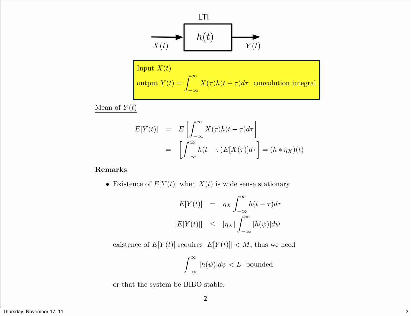
h(t)

LTI

Y (t)X(t)

Input X(t)

output Y (t) =

Z 1

�1X(⌧)h(t� ⌧)d⌧ convolution integral

Mean of Y (t)

E[Y (t)] = E

Z 1

�1X(⌧)h(t� ⌧)d⌧

�

=

Z 1

�1h(t� ⌧)E[X(⌧)]d⌧

�= (h ⇤ ⌘X)(t)

Remarks

• Existence of E[Y (t)] when X(t) is wide sense stationary

E[Y (t)] = ⌘X

Z 1

�1h(t� ⌧)d⌧

|E[Y (t)]| |⌘X |Z 1

�1|h( )|d

existence of E[Y (t)] requires |E[Y (t)]| < M , thus we need

Z 1

�1|h( )|d < L bounded

or that the system be BIBO stable.


3

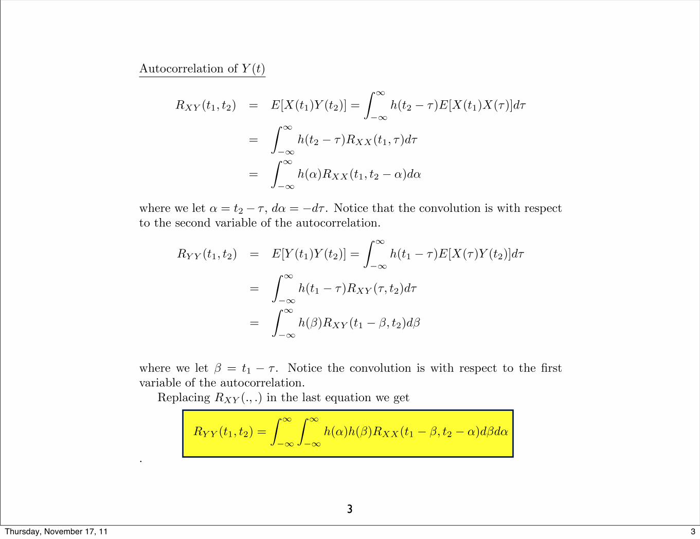
Autocorrelation of Y (t)

RXY (t1, t2) = E[X(t1)Y (t2)] =

Z 1

�1h(t2 � ⌧)E[X(t1)X(⌧)]d⌧

=

Z 1

�1h(t2 � ⌧)RXX(t1, ⌧)d⌧

=

Z 1

�1h(↵)RXX(t1, t2 � ↵)d↵

where we let ↵ = t2 � ⌧ , d↵ = �d⌧ . Notice that the convolution is with respect

to the second variable of the autocorrelation.

RY Y (t1, t2) = E[Y (t1)Y (t2)] =

Z 1

�1h(t1 � ⌧)E[X(⌧)Y (t2)]d⌧

=

Z 1

�1h(t1 � ⌧)RXY (⌧, t2)d⌧

=

Z 1

�1h(�)RXY (t1 � �, t2)d�

where we let � = t1 � ⌧ . Notice the convolution is with respect to the first

variable of the autocorrelation.

Replacing RXY (., .) in the last equation we get

RY Y (t1, t2) =

Z 1

�1

Z 1

�1h(↵)h(�)RXX(t1 � �, t2 � ↵)d�d↵

.


4

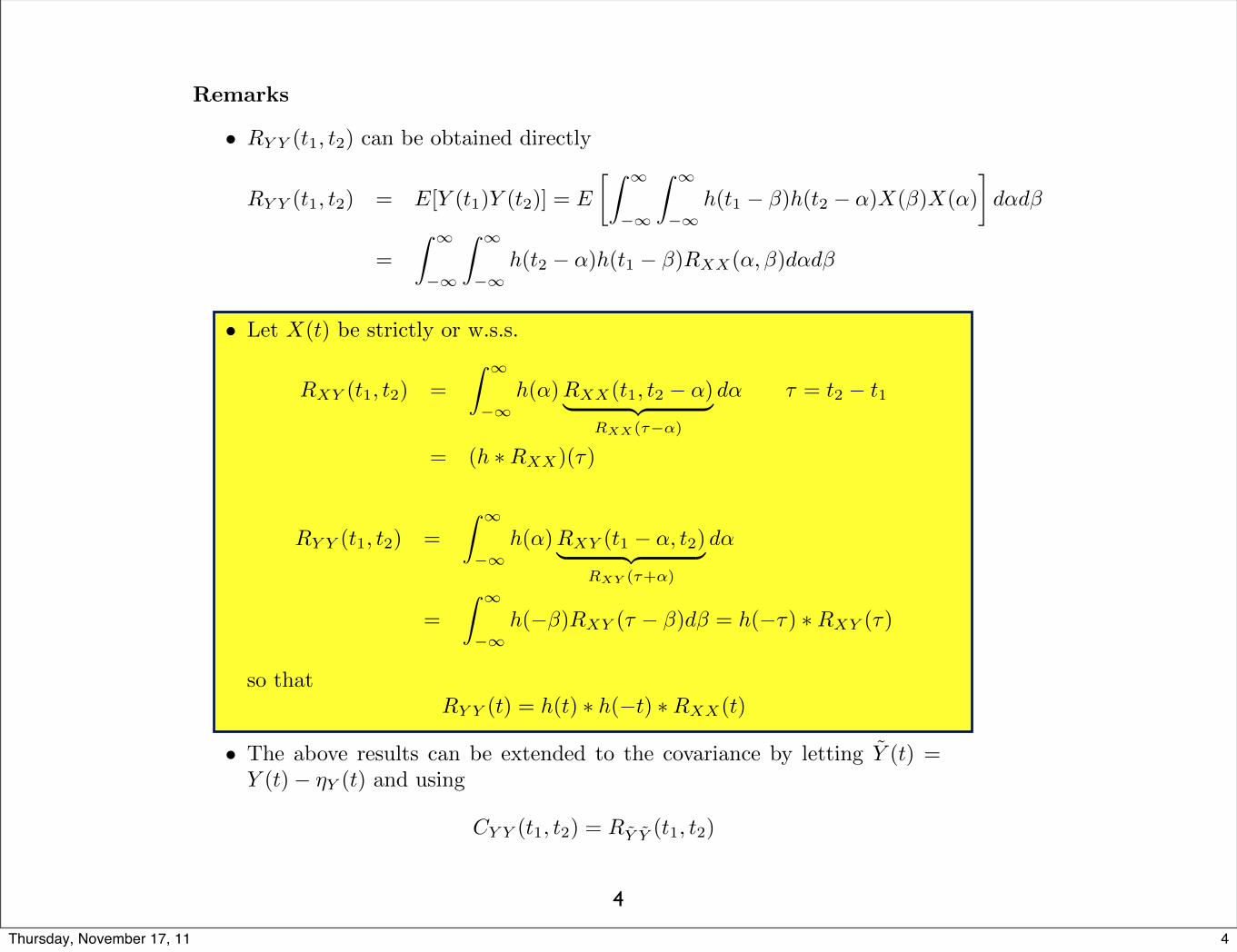
Remarks

• RY Y (t1, t2) can be obtained directly

RY Y (t1, t2) = E[Y (t1)Y (t2)] = E

Z 1

�1

Z 1

�1h(t1 � �)h(t2 � ↵)X(�)X(↵)

�d↵d�

=

Z 1

�1

Z 1

�1h(t2 � ↵)h(t1 � �)RXX(↵,�)d↵d�

• Let X(t) be strictly or w.s.s.

RXY (t1, t2) =

Z 1

�1h(↵)RXX(t1, t2 � ↵)| {z }

RXX(⌧�↵)

d↵ ⌧ = t2 � t1

= (h ⇤RXX)(⌧)

RY Y (t1, t2) =

Z 1

�1h(↵)RXY (t1 � ↵, t2)| {z }

RXY (⌧+↵)

d↵

=

Z 1

�1h(��)RXY (⌧ � �)d� = h(�⌧) ⇤RXY (⌧)

so that

RY Y (t) = h(t) ⇤ h(�t) ⇤RXX(t)

• The above results can be extended to the covariance by letting

˜Y (t) =

Y (t)� ⌘Y (t) and using

CY Y (t1, t2) = RY Y (t1, t2)


5

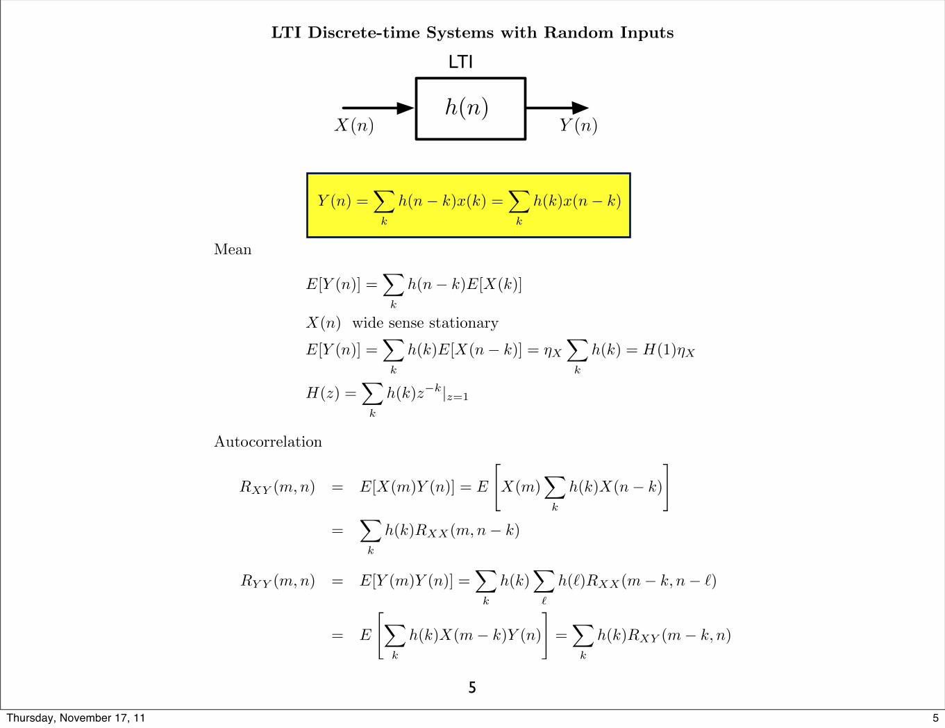
LTI

h(n)X(n) Y (n)

LTI Discrete-time Systems with Random Inputs

Y (n) =X

k

h(n� k)x(k) =X

k

h(k)x(n� k)

Mean

E[Y (n)] =X

k

h(n� k)E[X(k)]

X(n) wide sense stationary

E[Y (n)] =X

k

h(k)E[X(n� k)] = ⌘XX

k

h(k) = H(1)⌘X

H(z) =X

k

h(k)z�k|z=1

Autocorrelation

RXY (m,n) = E[X(m)Y (n)] = E

"X(m)

X

k

h(k)X(n� k)

#

=

X

k

h(k)RXX(m,n� k)

RY Y (m,n) = E[Y (m)Y (n)] =X

k

h(k)X

`

h(`)RXX(m� k, n� `)

= E

"X

k

h(k)X(m� k)Y (n)

#=

X

k

h(k)RXY (m� k, n)


6

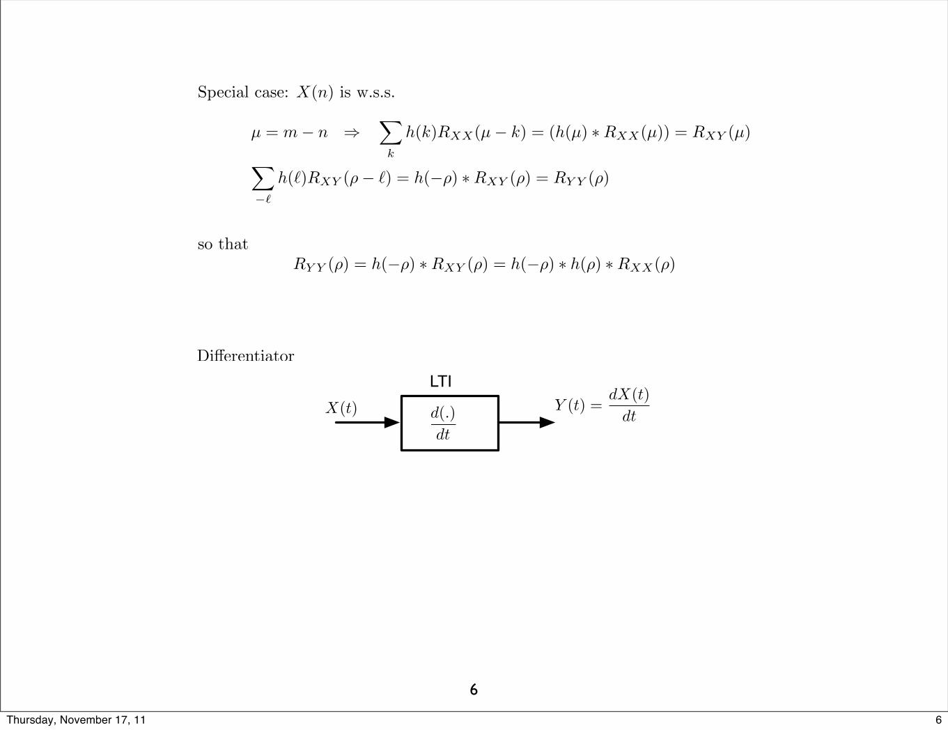
Special case: X(n) is w.s.s.

µ = m� n )X

k

h(k)RXX(µ� k) = (h(µ) ⇤RXX(µ)) = RXY (µ)

X

�`

h(`)RXY (⇢� `) = h(�⇢) ⇤RXY (⇢) = RY Y (⇢)

so that

RY Y (⇢) = h(�⇢) ⇤RXY (⇢) = h(�⇢) ⇤ h(⇢) ⇤RXX(⇢)

Di↵erentiator

LTI Y (t) =

dX(t)

dtX(t) d(.)

dt


7

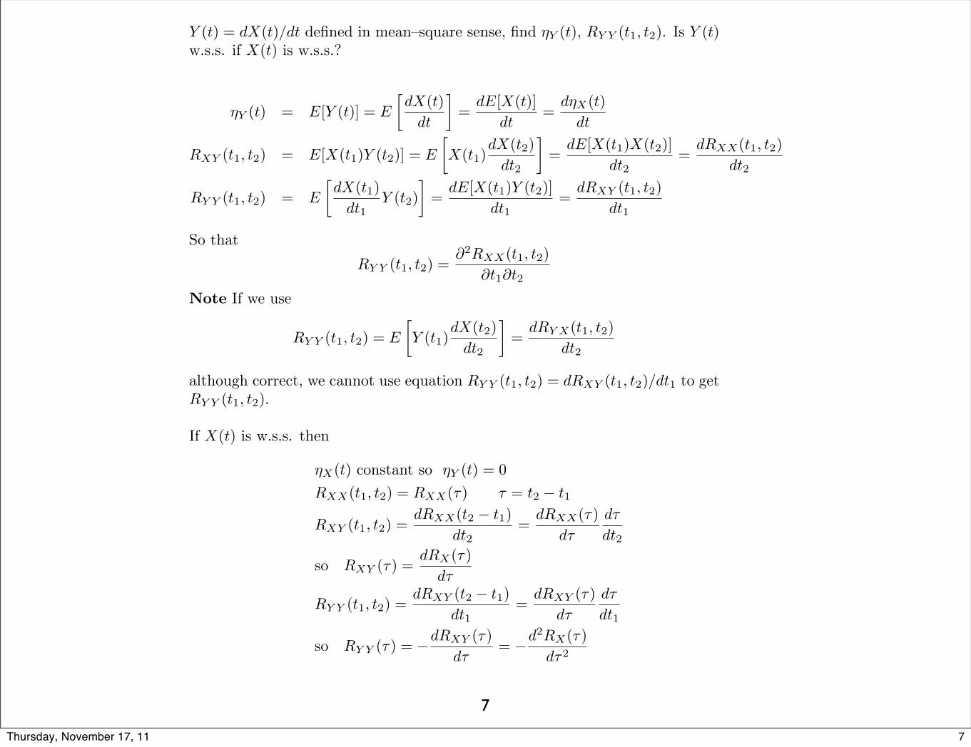
Y (t) = dX(t)/dt defined in mean–square sense, find ⌘Y (t), RY Y (t1, t2). Is Y (t)w.s.s. if X(t) is w.s.s.?

⌘Y (t) = E[Y (t)] = E

dX(t)

dt

�=

dE[X(t)]

dt=

d⌘X(t)

dt

RXY (t1, t2) = E[X(t1)Y (t2)] = E

X(t1)

dX(t2)

dt2

�=

dE[X(t1)X(t2)]

dt2=

dRXX(t1, t2)

dt2

RY Y (t1, t2) = E

dX(t1)

dt1Y (t2)

�=

dE[X(t1)Y (t2)]

dt1=

dRXY (t1, t2)

dt1

So that

RY Y (t1, t2) =@2RXX(t1, t2)

@t1@t2

Note If we use

RY Y (t1, t2) = E

Y (t1)

dX(t2)

dt2

�=

dRY X(t1, t2)

dt2

although correct, we cannot use equation RY Y (t1, t2) = dRXY (t1, t2)/dt1 to get

RY Y (t1, t2).

If X(t) is w.s.s. then

⌘X(t) constant so ⌘Y (t) = 0

RXX(t1, t2) = RXX(⌧) ⌧ = t2 � t1

RXY (t1, t2) =dRXX(t2 � t1)

dt2=

dRXX(⌧)

d⌧

d⌧

dt2

so RXY (⌧) =dRX(⌧)

d⌧

RY Y (t1, t2) =dRXY (t2 � t1)

dt1=

dRXY (⌧)

d⌧

d⌧

dt1

so RY Y (⌧) = �dRXY (⌧)

d⌧= �d2RX(⌧)

d⌧2


8

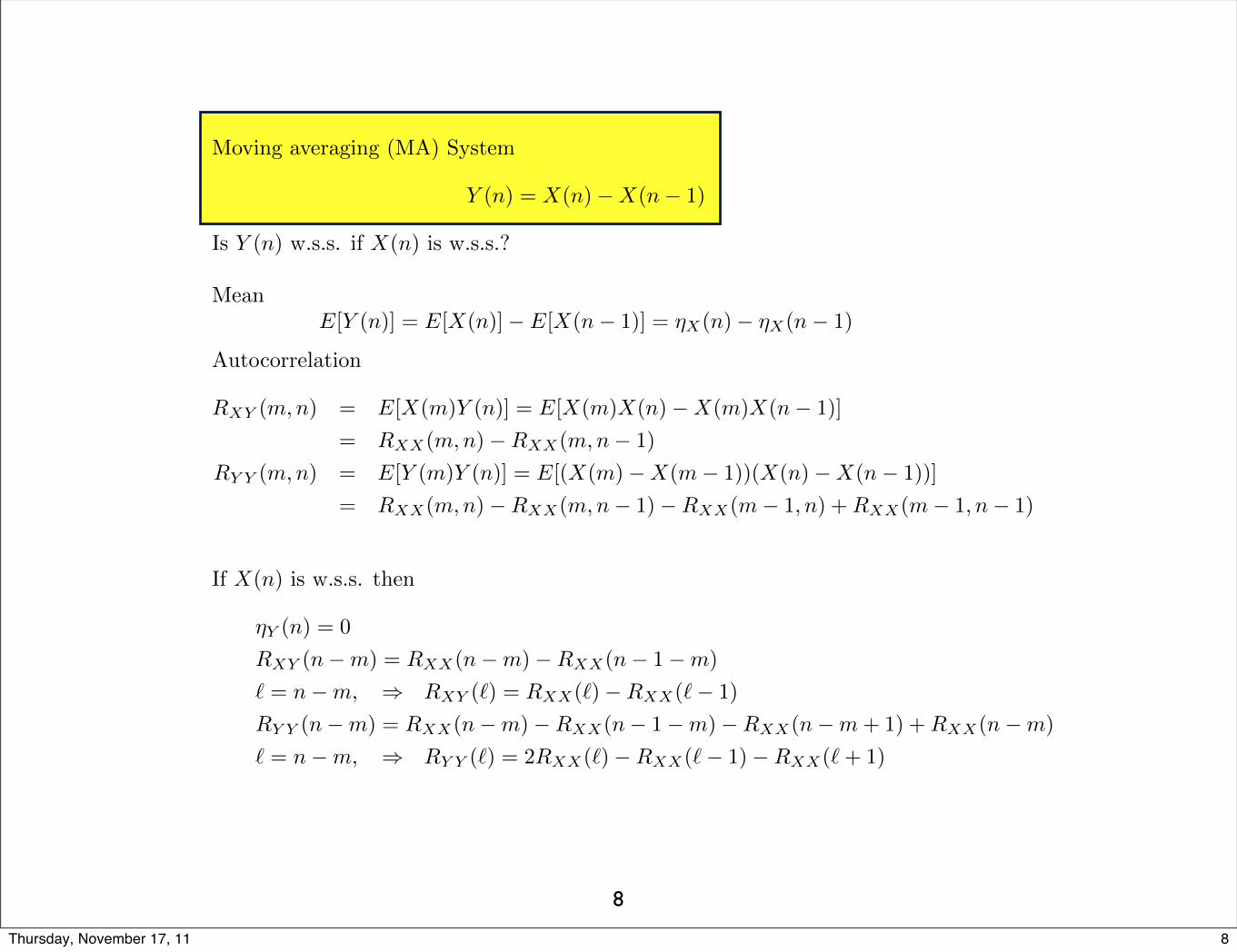
Moving averaging (MA) System

Y (n) = X(n)�X(n� 1)

Is Y (n) w.s.s. if X(n) is w.s.s.?

Mean

E[Y (n)] = E[X(n)]� E[X(n� 1)] = ⌘X(n)� ⌘X(n� 1)

Autocorrelation

RXY (m,n) = E[X(m)Y (n)] = E[X(m)X(n)�X(m)X(n� 1)]

= RXX(m,n)�RXX(m,n� 1)

RY Y (m,n) = E[Y (m)Y (n)] = E[(X(m)�X(m� 1))(X(n)�X(n� 1))]

= RXX(m,n)�RXX(m,n� 1)�RXX(m� 1, n) +RXX(m� 1, n� 1)

If X(n) is w.s.s. then

⌘Y (n) = 0

RXY (n�m) = RXX(n�m)�RXX(n� 1�m)

` = n�m, ) RXY (`) = RXX(`)�RXX(`� 1)

RY Y (n�m) = RXX(n�m)�RXX(n� 1�m)�RXX(n�m+ 1) +RXX(n�m)

` = n�m, ) RY Y (`) = 2RXX(`)�RXX(`� 1)�RXX(`+ 1)


9

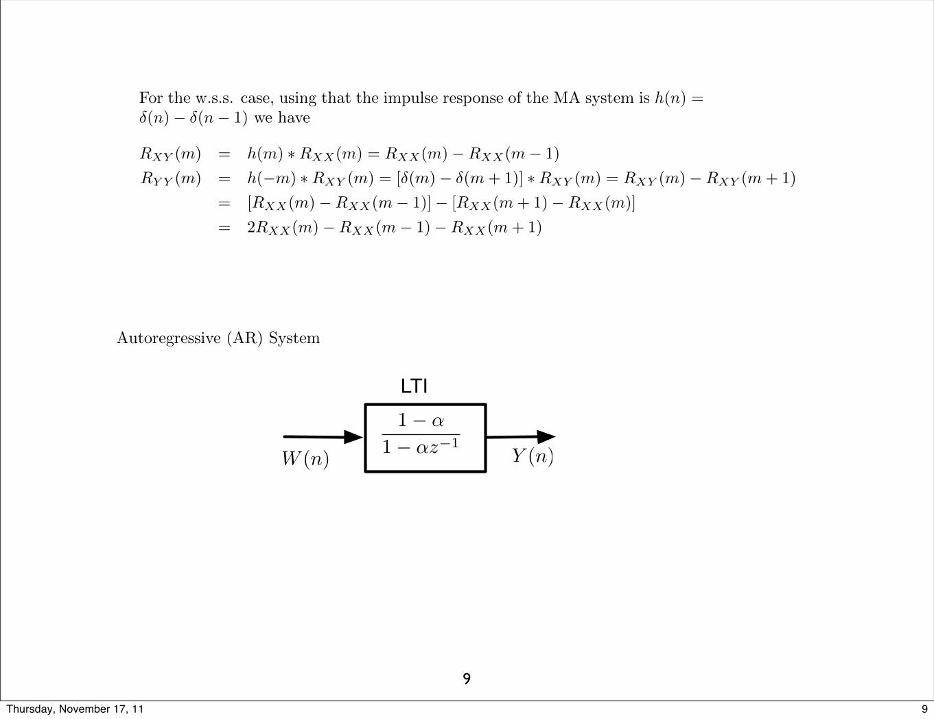
For the w.s.s. case, using that the impulse response of the MA system is h(n) =�(n)� �(n� 1) we have

RXY (m) = h(m) ⇤RXX(m) = RXX(m)�RXX(m� 1)

RY Y (m) = h(�m) ⇤RXY (m) = [�(m)� �(m+ 1)] ⇤RXY (m) = RXY (m)�RXY (m+ 1)

= [RXX(m)�RXX(m� 1)]� [RXX(m+ 1)�RXX(m)]

= 2RXX(m)�RXX(m� 1)�RXX(m+ 1)

Autoregressive (AR) System

LTI

Y (n)W (n)

1� �

1� �z�1


10

Y (n) = ↵Y (n� 1) + (1� ↵)W (n)

W (n) is w.s.s.

If we let z�1be equivalent to a delay then we have that the transfer function

of the system is

H(z) =1� ↵

1� ↵z�1= (1� ↵)

1X

n=0

↵nz�n

h(n) = (1� ↵)↵nu(n)

The input/output di↵erence equation is equivalent to

Y (n) =1X

k=0

h(k)W (n� k)

Then

E[Y (n)] =

1X

k=0

h(k)E[W (n� k)] = ⌘W

1X

k=0

h(k) = ⌘WH(1)

RWY (m,m+m0)| {z }RWY (m0)

=

X

k

h(k)RWW (m,m+m0 � k)| {z }RWW (m0�k)

RY Y (m,m+m0)| {z }RY Y (m0)

=

X

k

X

`

h(k)h(`)RWW (m0 � k + `)

Suppose W (n) is white noise

RWW (m) = �(m)

RWY (m) =

X

k

h(k)�(m� k) = h(m)

RY Y (m) = h(�m) ⇤RWY (m) = h(�m) ⇤ h(m)

Notice that RWY (m) is non-symmetric (zero for negative m) while RY Y (m) is

symmetric.


11

Di↵erence equation for RY Y (.) Consider the AR system

Y (n) = ↵Y (n� 1) + (1� ↵)W (n) (1)

such that if W (n) is w.s.s. the output Y (n) is also w.s.s. Multiply equation (1)

by Y (n+m) to get

E[Y (n)Y (n+m)] = ↵E[Y (n� 1)Y (n+m)] + (1� ↵)E[W (n)Y (n+m)]

RY Y (m) = ↵RY Y (m� 1) + (1� ↵)RWY (n,m+ n)

if W (n),Y (n) are jointly wide sense stationary, i.e., RWY (n,m+n) = RWY (m)

then a di↵erence equation to obtain the autocorrelation is

RY Y (m) = ↵RY Y (m� 1) + (1� ↵)RWY (m)


12

Continuous-time Stationary Processes

Autocorrelation: measures relation of X(t) and X(t+ ⌧) for a lag ⌧

RX(⌧) = E[X(t)X(t+ ⌧)]

Properties

• RX(⌧) is even function of lag ⌧

RX(⌧) = E[X(t)X(t+ ⌧)] = E[X(t+ ⌧)X(t)] = RX(�⌧)

• |RX(⌧)| RX(0), indeed

0 E[(X(t+ ⌧)�X(t))2] = E[X2(t+ ⌧)] + E[X2

(t)]� 2E[X(t+ ⌧)X(t)]

= 2RX(0)� 2RX(⌧) ) RX(0) � RX(⌧)

• If there is a T > 0 such that RX(0) = RX(T ) then RX(⌧) is periodic.

• RX(⌧) is a positive definite function.

Power Spectral Density — Continuous-time Random Processes

If RX(⌧) is the autocorrelation of a w.s.s. process X(t) then SX(⌦) (or SX(f),⌦ = 2⇡f) is the power spectral density of X(t) and given by

SX(⌦) =

Z 1

�1RX(⌧)e�j⌦⌧d⌧

RX(⌧) =

1

2⇡

Z 1

�1SX(⌦)ej⌦⌧d⌦

=

Z 1

�1SX(f)ej2⇡⌧df


13

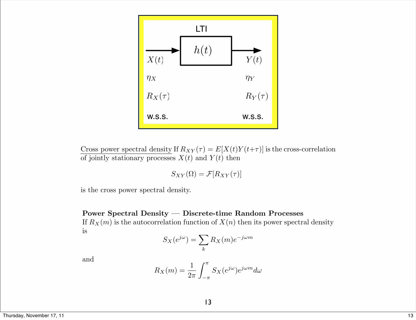
h(t)

LTI

Y (t)X(t)

⌘X ⌘Y

RY (�)RX(�)

w.s.s. w.s.s.

Power Spectral Density — Discrete-time Random Processes

If RX(m) is the autocorrelation function of X(n) then its power spectral density

is

SX(ej!) =X

k

RX(m)e�j!m

and

RX(m) =

1

2⇡

Z ⇡

�⇡SX(ej!)ej!md!

Cross power spectral density IfRXY (⌧) = E[X(t)Y (t+⌧)] is the cross-correlationof jointly stationary processes X(t) and Y (t) then

SXY (⌦) = F [RXY (⌧)]

is the cross power spectral density.


14

Properties of SX(⌦)

If X(t) is a real-valued process

• SX(⌦) is a real function

SX(⌦) =

Z 1

�1RX(⌧)e�j⌦⌧d⌧

=

Z 1

�1RX(⌧) cos(⌦⌧)d⌧ � j

Z 1

�1RX(⌧) sin(⌦⌧)d⌧

| {z }0

• SX(⌦) is an even function of ⌦

SX(⌦) = SX(�⌦) because cos(⌦⌧) = cos(�⌦⌧)

(If X(t) is not real-valued, then SX(⌦) is not necessarily even.)

• SX(⌦) � 0, i.e., it has the positive characteristics of a power density

function.

Remarks

• The Fourier transform cannot be applied directly to X(t) because its FT

would not exist.

• Similar properties for SX(ej!).

If X(t), a w.s.s. random process, is the input of a LTI system with impulse

response h(t), the output Y (t) is also w.s.s. random process with autocorrelation

RY (⌧) = h(�⌧) ⇤ h(⌧) ⇤RX(⌧) and power spectral density

SY (⌦) = H(⌦)

⇤H(⌦)SX(⌦) = |H(⌦)|2SX(⌦)


15

Remark

• For a discrete-time system

SY (ej!) = |H(ej!)|2SX(ej!)

• For cross-correlation

RXY (⌧) = h(⌧) ⇤RX(⌧)

SXY (⌦) = H(⌦)SX(⌦)

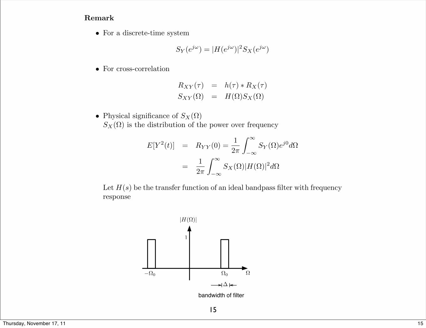
• Physical significance of SX(⌦)

SX(⌦) is the distribution of the power over frequency

E[Y 2(t)] = RY Y (0) =

1

2⇡

Z 1

�1SY (⌦)e

j0d⌦

=

1

2⇡

Z 1

�1SX(⌦)|H(⌦)|2d⌦

LetH(s) be the transfer function of an ideal bandpass filter with frequency

response

|H(�)|

�

⌦0�⌦0

bandwidth of filter

⌦

1


16

SY (⌦) = SX(⌦)|H(⌦)|2

⇡⇢

SX(⌦0) |⌦± ⌦0| �/20 otherwise

We thus have

E[Y 2(t)] = RY (0) = 2�SX(⌦0)

where the units of � are rad/sec and those of RY (0) are power, so that SX(.)has as units power/(rad/sec) or power density over frequency. Notice also that

E[Y 2(t)] = 2�SX(⌦0) � 0

indicating that as a density function SX(⌦0) � 0.


17

Other properties of SX(⌦)

• Let Y (t) = aX1(t) + bX2(t) where Xi(t), i = 1, 2 are orthogonal w.s.s.

RY (⌧) = E[Y (t)Y (t+ ⌧)] = E[(aX1(t) + bX2(t))(aX1(t+ ⌧) + bX2(t+ ⌧))]

= a2RX1(⌧) + b2RX2(⌧)

SY (⌦) = a2SX1(⌦) + b2SX2(⌦)

• Let Y (t) = dX(t)dt , which can be thought of X(t) being the input of a LTI

system with H(⌦) = j⌦ then

SY (⌦) = |j⌦|2SX(⌦) = ⌦

2SX(⌦)

This is equivalent to using the derivative property of the Fourier transform

RX(⌧) $ SX(⌦)

d2RX(⌧)

dt2$ (j⌦)2SX(⌦) = �⌦

2SX(⌦)

RY (⌧) = �d2RX(⌧)

dt2$ ⌦

2SX(⌦) = SY (⌦)

• Consider the modulation process: X(t) input w.s.s. process, modulates a

complex exponential ej⌦0tso that the output is

Y (t) = X(t)ej⌦0t

which is a complex process

RY (⌧) = E[Y (t)Y ⇤(t+ ⌧)] = E[X(t)X(t+ ⌧)ej⌦0(t�t�⌧)

]

= RX(⌧)e�j⌦0⌧

so that

SY (⌦) = SX(⌦+ ⌦0)

i.e., shifted in frequency to ⌦0. SY (⌦) is not even because Y (t) is complex.


18

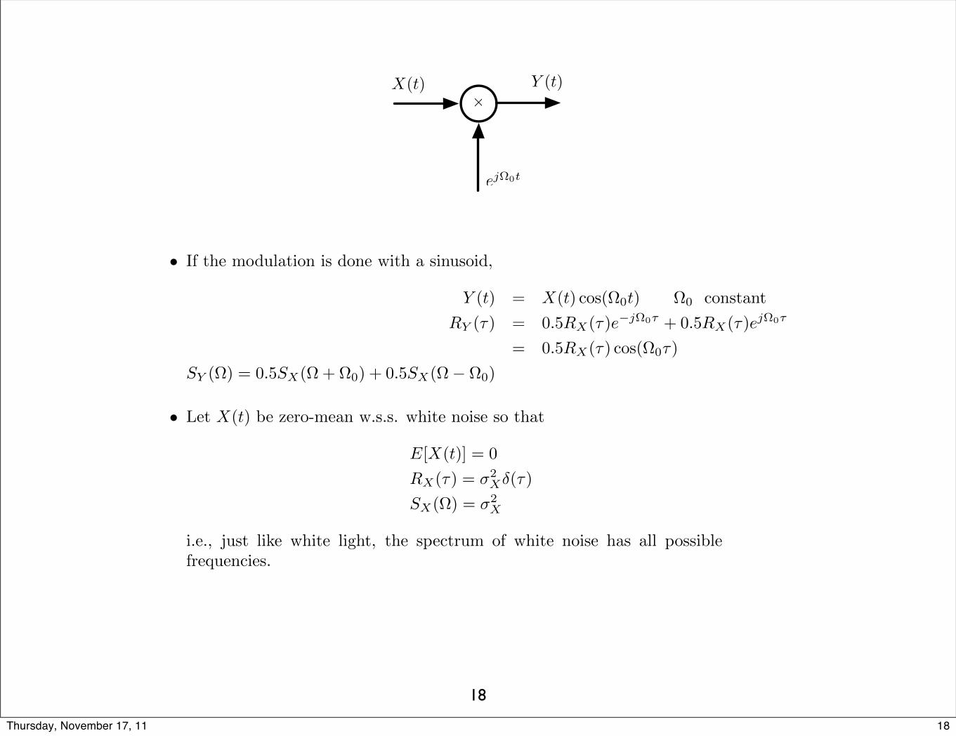
⇥X(t) Y (t)

ej⌦0t

• If the modulation is done with a sinusoid,

Y (t) = X(t) cos(⌦0t) ⌦0 constant

RY (⌧) = 0.5RX(⌧)e�j⌦0⌧+ 0.5RX(⌧)ej⌦0⌧

= 0.5RX(⌧) cos(⌦0⌧)

SY (⌦) = 0.5SX(⌦+ ⌦0) + 0.5SX(⌦� ⌦0)

• Let X(t) be zero-mean w.s.s. white noise so that

E[X(t)] = 0

RX(⌧) = �2X�(⌧)

SX(⌦) = �2X

i.e., just like white light, the spectrum of white noise has all possible

frequencies.


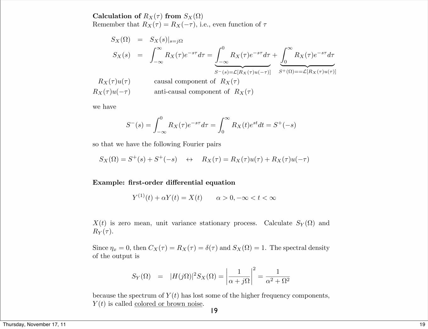
19

Calculation of RX

(⌧) from SX

(⌦)

Remember that RX

(⌧) = RX

(�⌧), i.e., even function of ⌧

SX

(⌦) = SX

(s)|s=j⌦

SX

(s) =

Z 1

�1R

X

(⌧)e�s⌧d⌧ =

Z 0

�1R

X

(⌧)e�s⌧d⌧

| {z }S

�(s)=L[RX(⌧)u(�⌧)]

+

Z 1

0R

X

(⌧)e�s⌧d⌧

| {z }S

+(⌦)==L[RX(⌧)u(⌧)]

RX

(⌧)u(⌧) causal component of RX

(⌧)

RX

(⌧)u(�⌧) anti-causal component of RX

(⌧)

we have

S�(s) =

Z 0

�1R

X

(⌧)e�s⌧d⌧ =

Z 1

0R

X

(t)estdt = S+(�s)

so that we have the following Fourier pairs

SX

(⌦) = S+(s) + S+

(�s) $ RX

(⌧) = RX

(⌧)u(⌧) +RX

(⌧)u(�⌧)

Example: first-order di↵erential equation

Y (1)(t) + ↵Y (t) = X(t) ↵ > 0,�1 < t < 1

X(t) is zero mean, unit variance stationary process. Calculate SY

(⌦) and

RY

(⌧).

Since ⌘x

= 0, then CX

(⌧) = RX

(⌧) = �(⌧) and SX

(⌦) = 1. The spectral density

of the output is

SY

(⌦) = |H(j⌦)|2SX

(⌦) =

��1

↵+ j⌦

��2

=

1

↵2+ ⌦

2

because the spectrum of Y (t) has lost some of the higher frequency components,

Y (t) is called colored or brown noise.


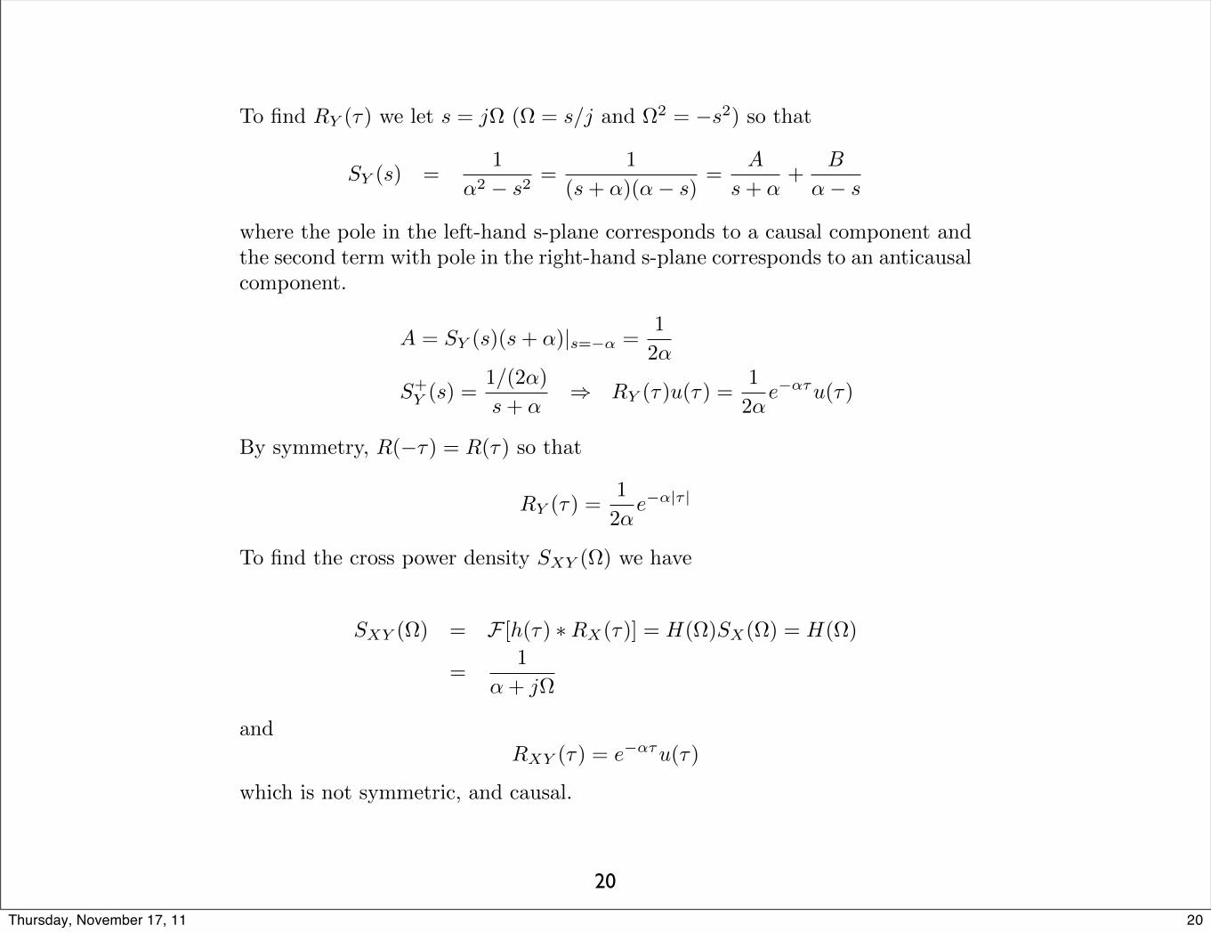
20

To find RY (⌧) we let s = j⌦ (⌦ = s/j and ⌦

2= �s2) so that

SY (s) =

1

↵2 � s2=

1

(s+ ↵)(↵� s)=

A

s+ ↵+

B

↵� s

where the pole in the left-hand s-plane corresponds to a causal component and

the second term with pole in the right-hand s-plane corresponds to an anticausal

component.

A = SY (s)(s+ ↵)|s=�↵ =

1

2↵

S+Y (s) =

1/(2↵)

s+ ↵) RY (⌧)u(⌧) =

1

2↵e�↵⌧u(⌧)

By symmetry, R(�⌧) = R(⌧) so that

RY (⌧) =1

2↵e�↵|⌧ |

To find the cross power density SXY (⌦) we have

SXY (⌦) = F [h(⌧) ⇤RX(⌧)] = H(⌦)SX(⌦) = H(⌦)

=

1

↵+ j⌦

and

RXY (⌧) = e�↵⌧u(⌧)

which is not symmetric, and causal.


21

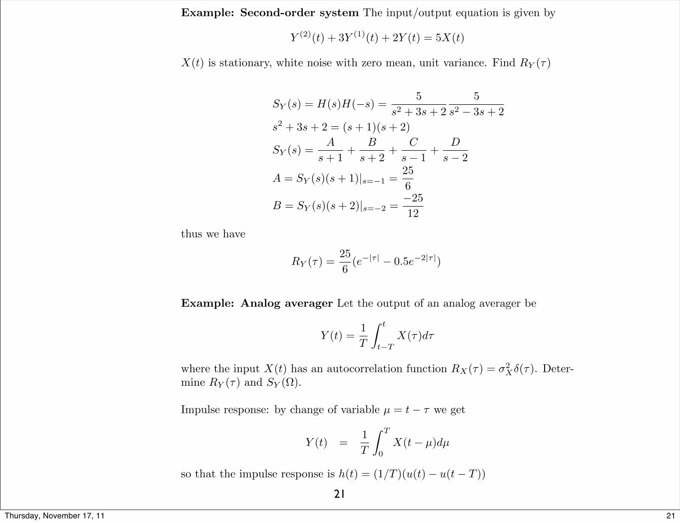
Example: Second-order system The input/output equation is given by

Y (2)(t) + 3Y (1)

(t) + 2Y (t) = 5X(t)

X(t) is stationary, white noise with zero mean, unit variance. Find RY (⌧)

SY (s) = H(s)H(�s) =5

s2 + 3s+ 2

5

s2 � 3s+ 2

s2 + 3s+ 2 = (s+ 1)(s+ 2)

SY (s) =A

s+ 1

+

B

s+ 2

+

C

s� 1

+

D

s� 2

A = SY (s)(s+ 1)|s=�1 =

25

6

B = SY (s)(s+ 2)|s=�2 =

�25

12

thus we have

RY (⌧) =25

6

(e�|⌧ | � 0.5e�2|⌧ |)

Example: Analog averager Let the output of an analog averager be

Y (t) =1

T

Z t

t�TX(⌧)d⌧

where the input X(t) has an autocorrelation function RX(⌧) = �2X�(⌧). Deter-

mine RY (⌧) and SY (⌦).

Impulse response: by change of variable µ = t� ⌧ we get

Y (t) =

1

T

Z T

0X(t� µ)dµ

so that the impulse response is h(t) = (1/T )(u(t)� u(t� T ))


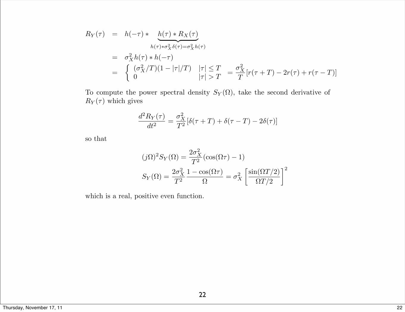
22

RY (⌧) = h(�⌧) ⇤ h(⌧) ⇤RX(⌧)| {z }h(⌧)⇤�2

X�(⌧)=�2Xh(⌧)

= �2Xh(⌧) ⇤ h(�⌧)

=

⇢(�2

X/T )(1� |⌧ |/T ) |⌧ | T0 |⌧ | > T

=

�2X

T[r(⌧ + T )� 2r(⌧) + r(⌧ � T )]

To compute the power spectral density SY (⌦), take the second derivative of

RY (⌧) which gives

d2RY (⌧)

dt2=

�2X

T 2[�(⌧ + T ) + �(⌧ � T )� 2�(⌧)]

so that

(j⌦)2SY (⌦) =2�2

X

T 2(cos(⌦⌧)� 1)

SY (⌦) =2�2

X

T 2

1� cos(⌦⌧)

⌦

= �2X

sin(⌦T/2)

⌦T/2

�2

which is a real, positive even function.


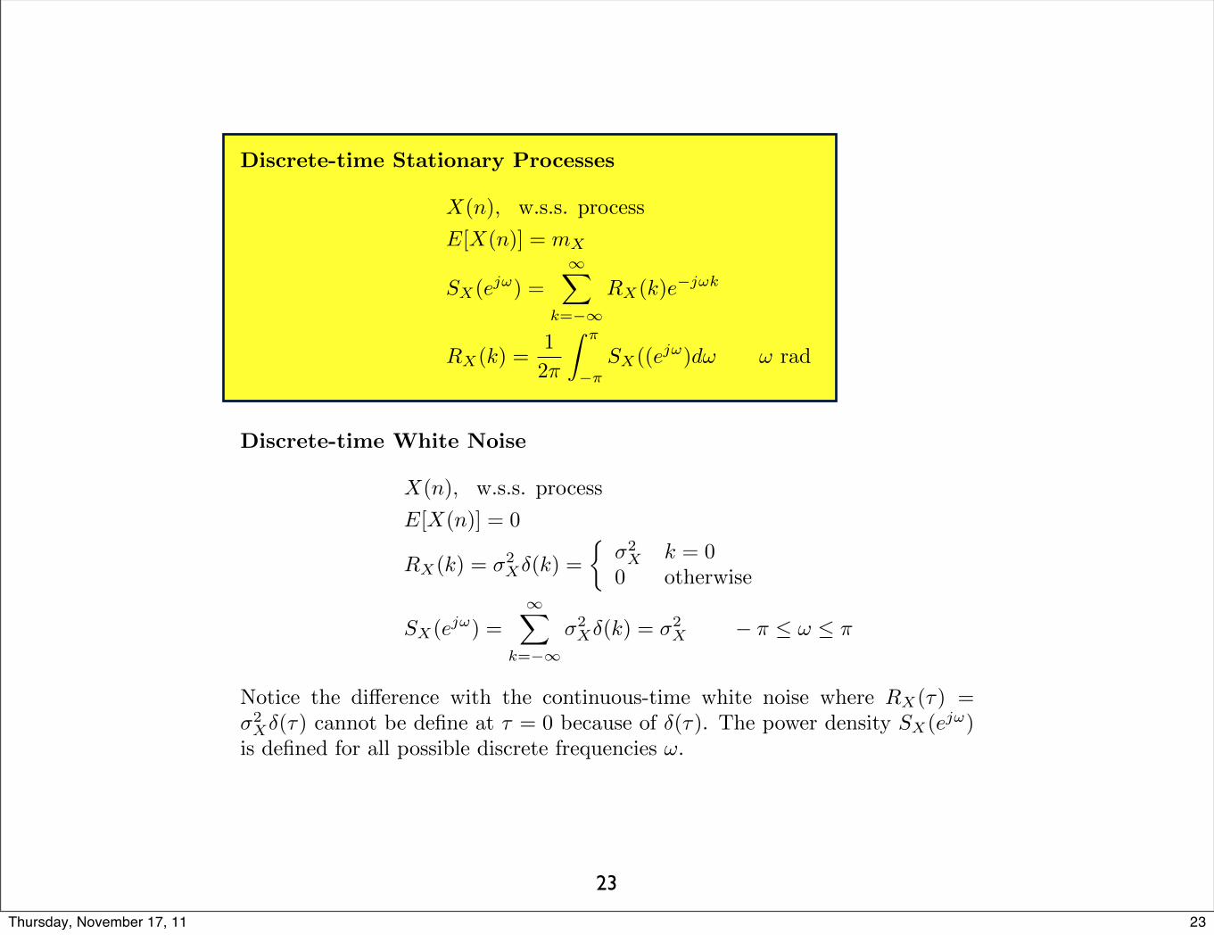
23

Discrete-time Stationary Processes

X(n), w.s.s. process

E[X(n)] = mX

SX(ej!) =1X

k=�1RX(k)e�j!k

RX(k) =1

2⇡

Z ⇡

�⇡SX((ej!)d! ! rad

Discrete-time White Noise

X(n), w.s.s. process

E[X(n)] = 0

RX(k) = �2X�(k) =

⇢�2X k = 0

0 otherwise

SX(ej!) =1X

k=�1�2X�(k) = �2

X � ⇡ ! ⇡

Notice the di↵erence with the continuous-time white noise where RX(⌧) =

�2X�(⌧) cannot be define at ⌧ = 0 because of �(⌧). The power density SX(ej!)

is defined for all possible discrete frequencies !.


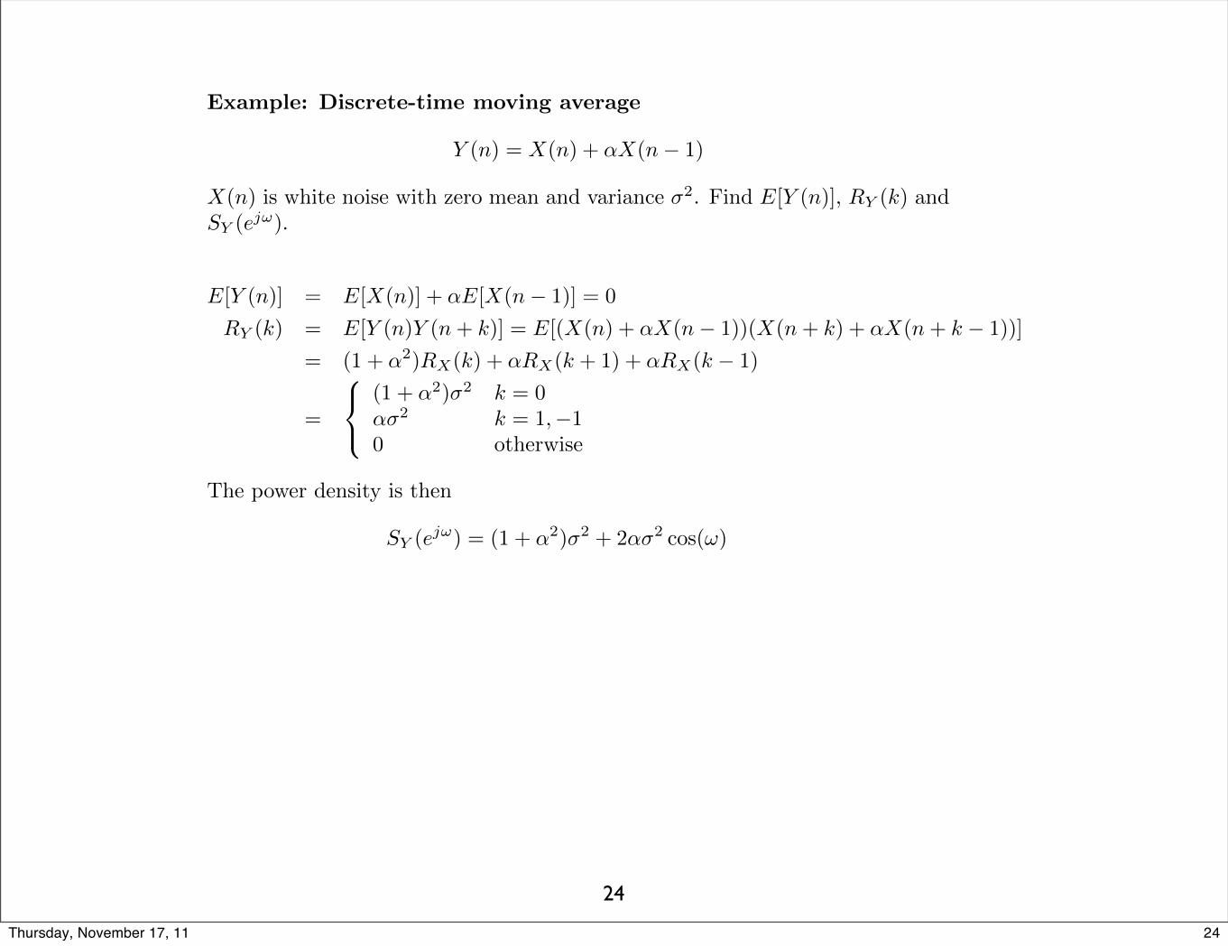
24

Example: Discrete-time moving average

Y (n) = X(n) + ↵X(n� 1)

X(n) is white noise with zero mean and variance �2. Find E[Y (n)], RY (k) and

SY (ej!).

E[Y (n)] = E[X(n)] + ↵E[X(n� 1)] = 0

RY (k) = E[Y (n)Y (n+ k)] = E[(X(n) + ↵X(n� 1))(X(n+ k) + ↵X(n+ k � 1))]

= (1 + ↵2)RX(k) + ↵RX(k + 1) + ↵RX(k � 1)

=

8<

:

(1 + ↵2)�2 k = 0

↵�2 k = 1,�1

0 otherwise

The power density is then

SY (ej!) = (1 + ↵2

)�2+ 2↵�2

cos(!)


Documents

Linear Time-invariant Systems with Random Inputslfch/EE2521/lecture10.pdfLinear Time-invariant Systems with Random Inputs Thursday, November 17, 11 1 2 h(t) LTI X(t) Y (t) Input X(t)