Embed Size (px)
Citation preview
Linear Time Constituency Parsing with
RNNs and Dynamic Programming
Juneki Hong 1 Liang Huang 1,2
1 Oregon State University2 Baidu Research Silicon Valley AI Lab
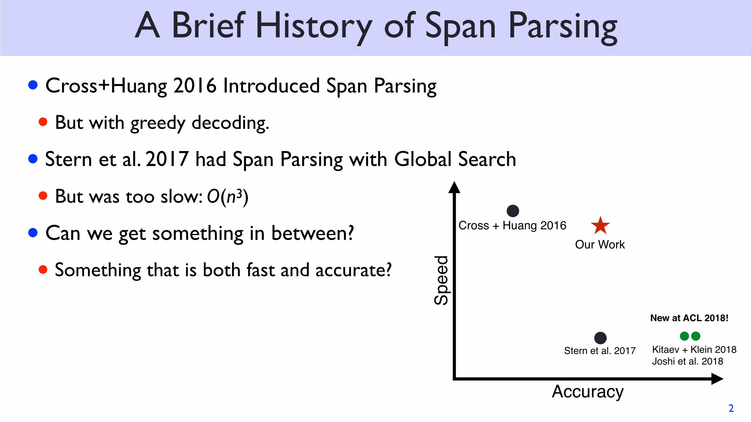
A Brief History of Span Parsing
• Cross+Huang 2016 Introduced Span Parsing
• But with greedy decoding.
• Stern et al. 2017 had Span Parsing with Global Search
• But was too slow: O(n3)
• Can we get something in between?
• Something that is both fast and accurate?
2Accuracy
Spee
d
Cross + Huang 2016
Stern et al. 2017
Our Work
Kitaev + Klein 2018Joshi et al. 2018
New at ACL 2018!
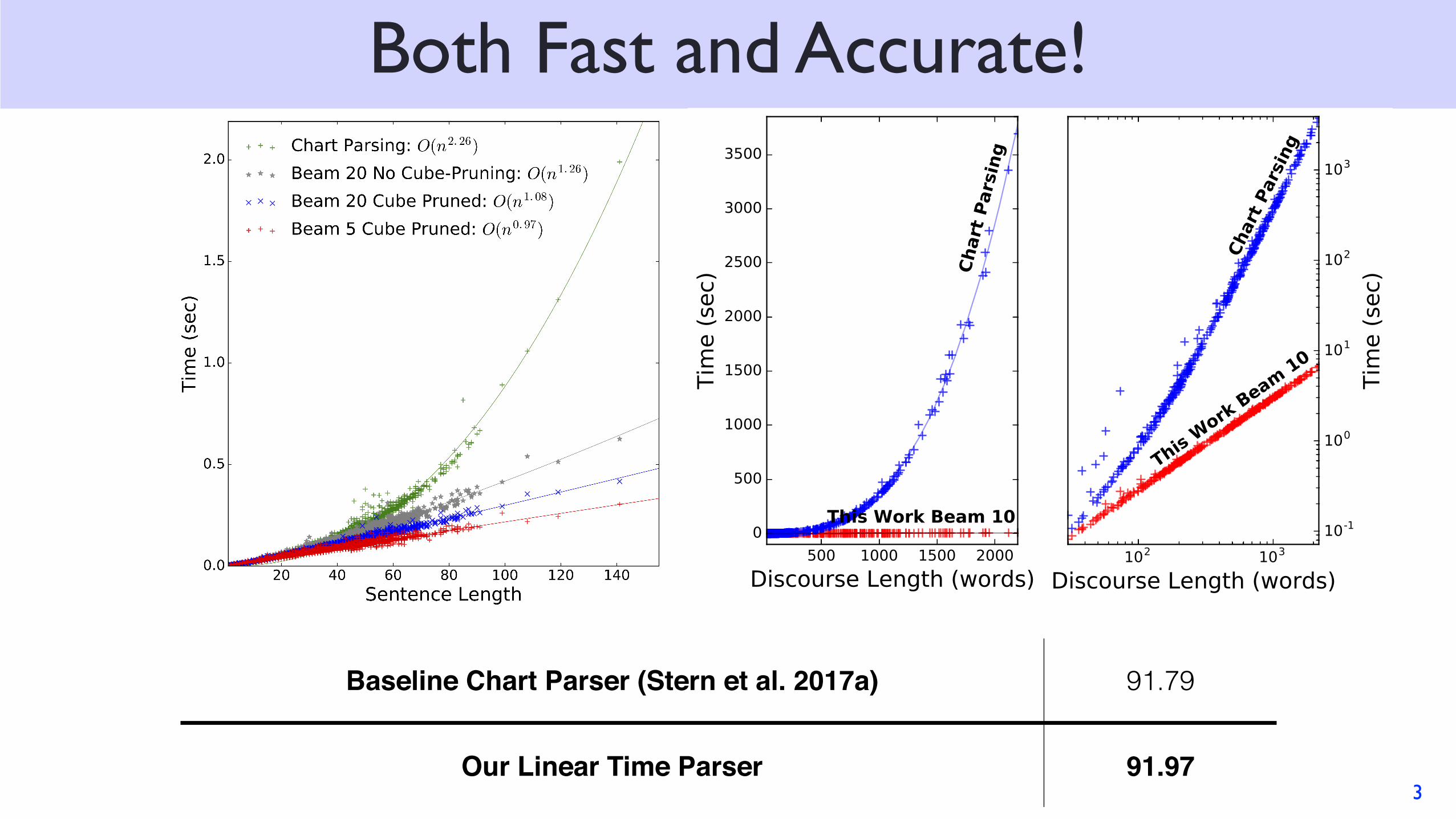
Both Fast and Accurate!
3
Baseline Chart Parser (Stern et al. 2017a) 91.79
Our Linear Time Parser 91.97
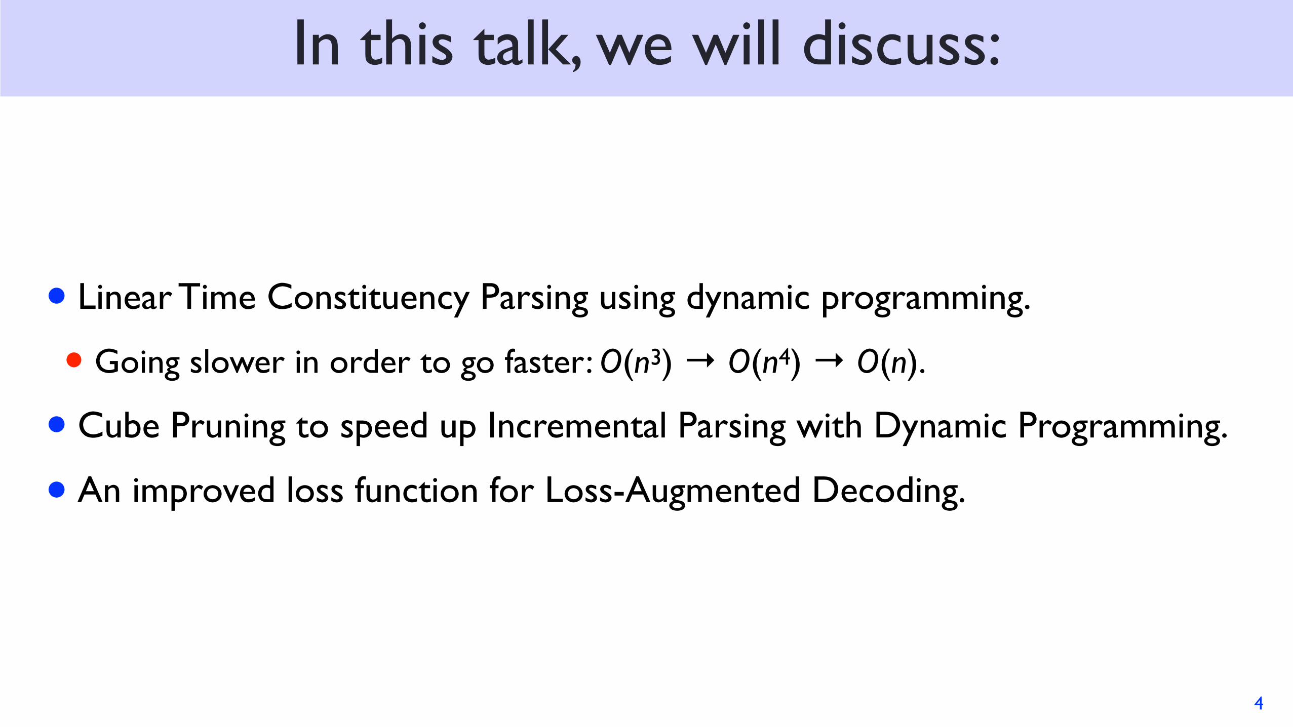
In this talk, we will discuss:
• Linear Time Constituency Parsing using dynamic programming.
• Going slower in order to go faster: O(n3) → O(n4) → O(n).
• Cube Pruning to speed up Incremental Parsing with Dynamic Programming.
• An improved loss function for Loss-Augmented Decoding.
4
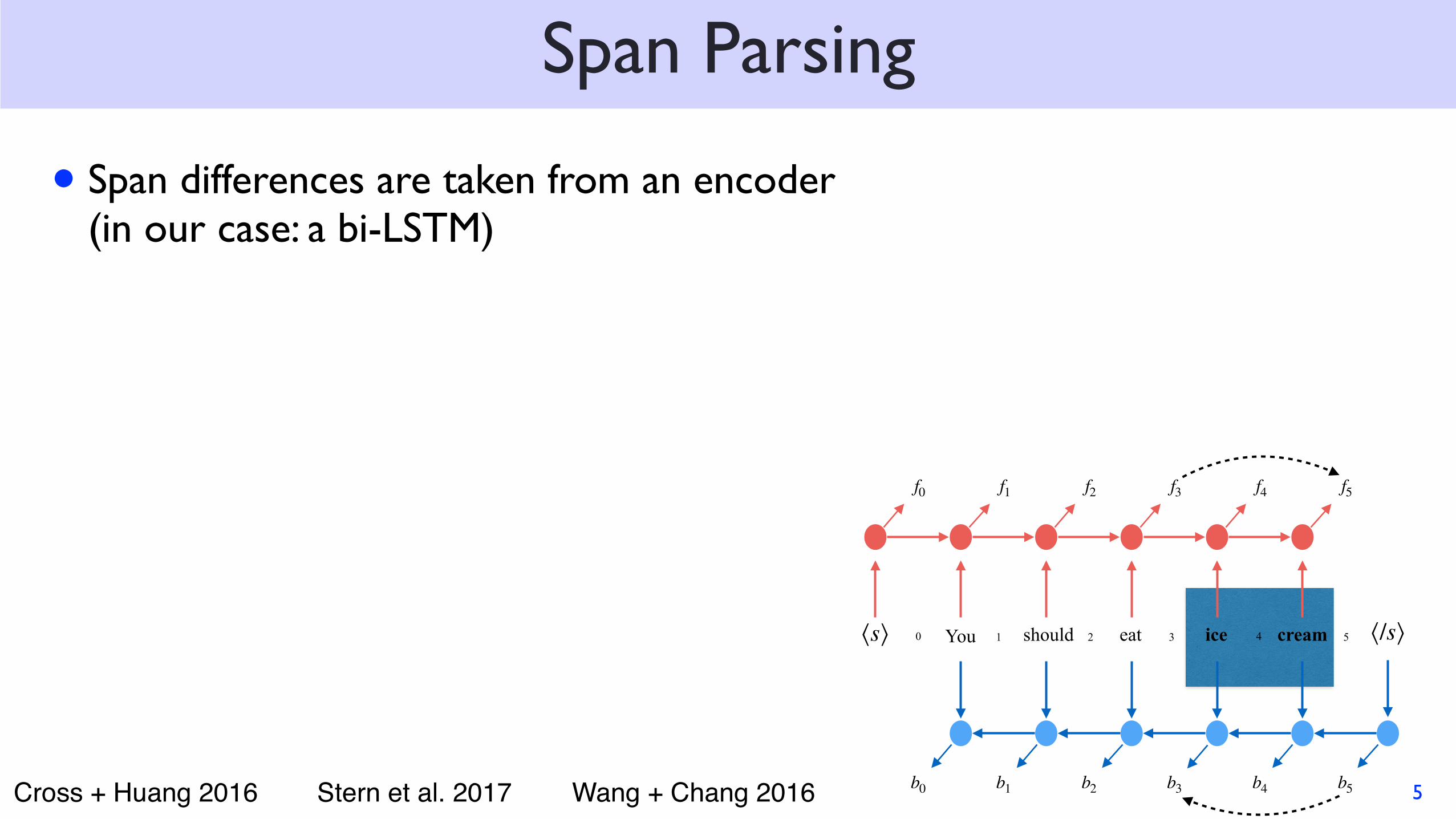
Span Parsing
• Span differences are taken from an encoder (in our case: a bi-LSTM)
5
⟨/s⟩⟨s⟩
f0 f1 f2 f3 f4 f5
b1 b2 b3 b4 b5b0
1 3 50 2 4You should eat ice cream
Cross + Huang 2016 Stern et al. 2017 Wang + Chang 2016
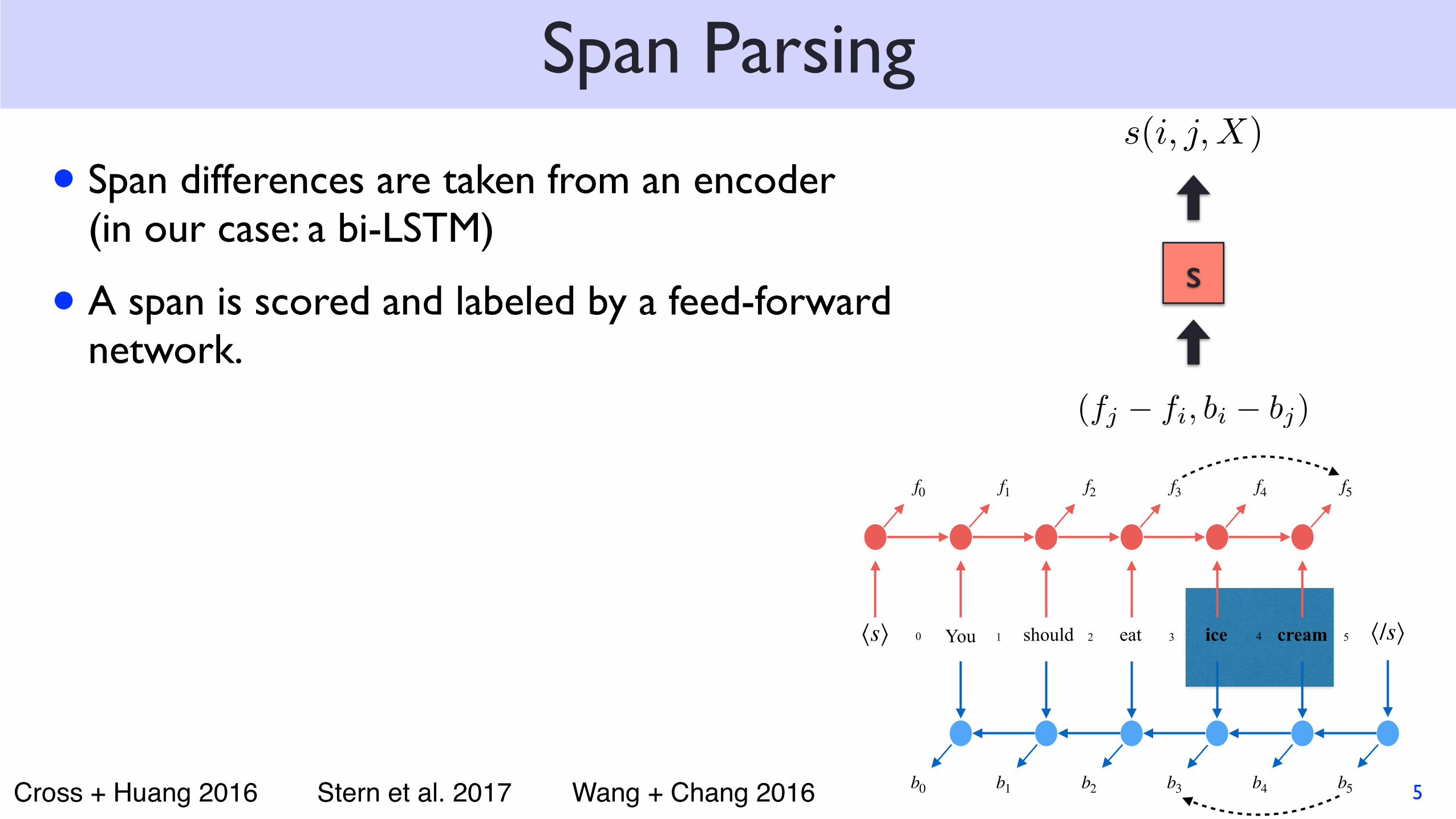
Span Parsing
• Span differences are taken from an encoder (in our case: a bi-LSTM)
• A span is scored and labeled by a feed-forward network.
5
s
(fj � fi, bi � bj)
s(i, j,X)
⟨/s⟩⟨s⟩
f0 f1 f2 f3 f4 f5
b1 b2 b3 b4 b5b0
1 3 50 2 4You should eat ice cream
Cross + Huang 2016 Stern et al. 2017 Wang + Chang 2016
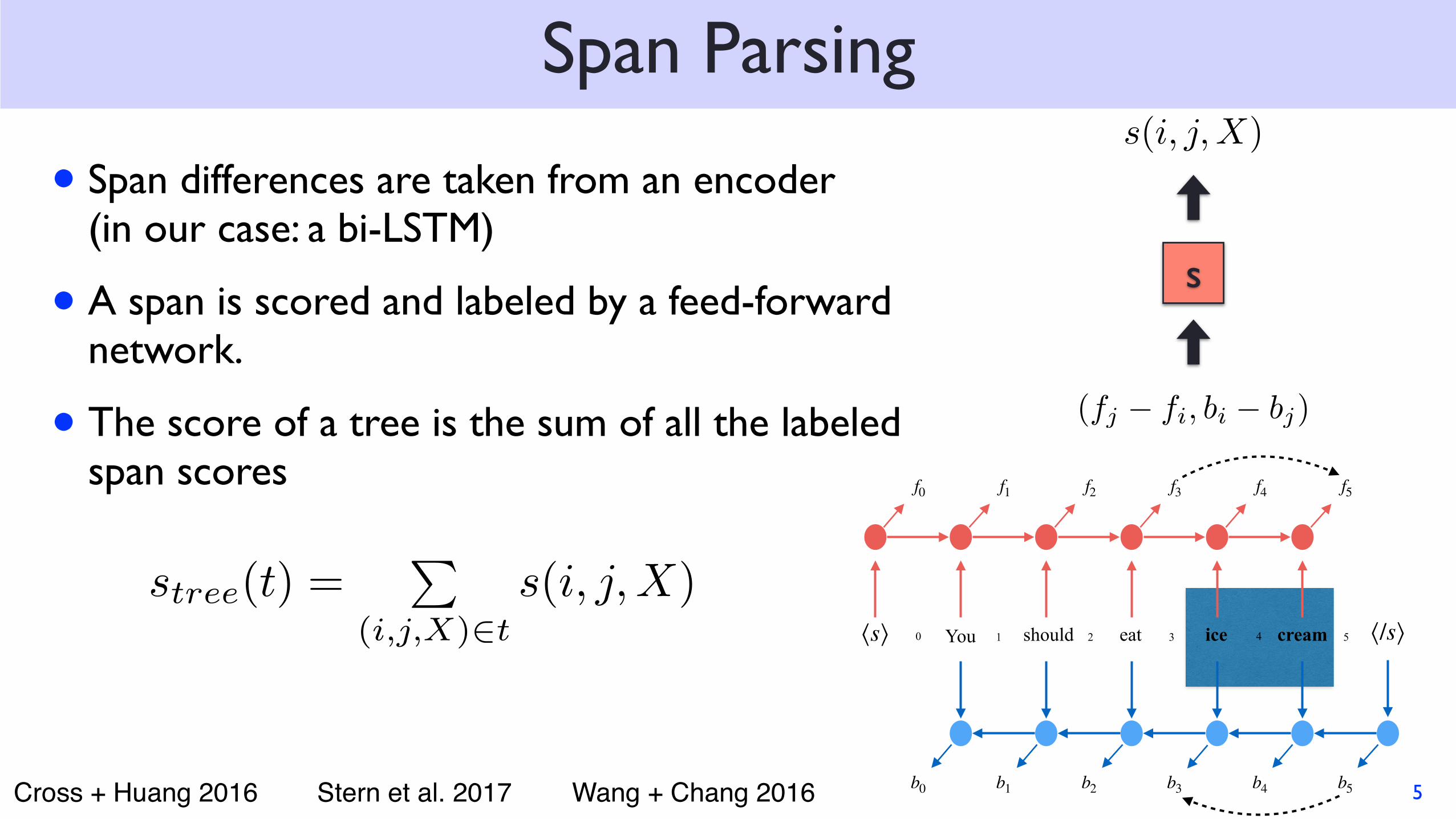
Span Parsing
• Span differences are taken from an encoder (in our case: a bi-LSTM)
• A span is scored and labeled by a feed-forward network.
• The score of a tree is the sum of all the labeled span scores
5
s
stree(t) =P
(i,j,X)2t
s(i, j,X)
(fj � fi, bi � bj)
s(i, j,X)
⟨/s⟩⟨s⟩
f0 f1 f2 f3 f4 f5
b1 b2 b3 b4 b5b0
1 3 50 2 4You should eat ice cream
Cross + Huang 2016 Stern et al. 2017 Wang + Chang 2016
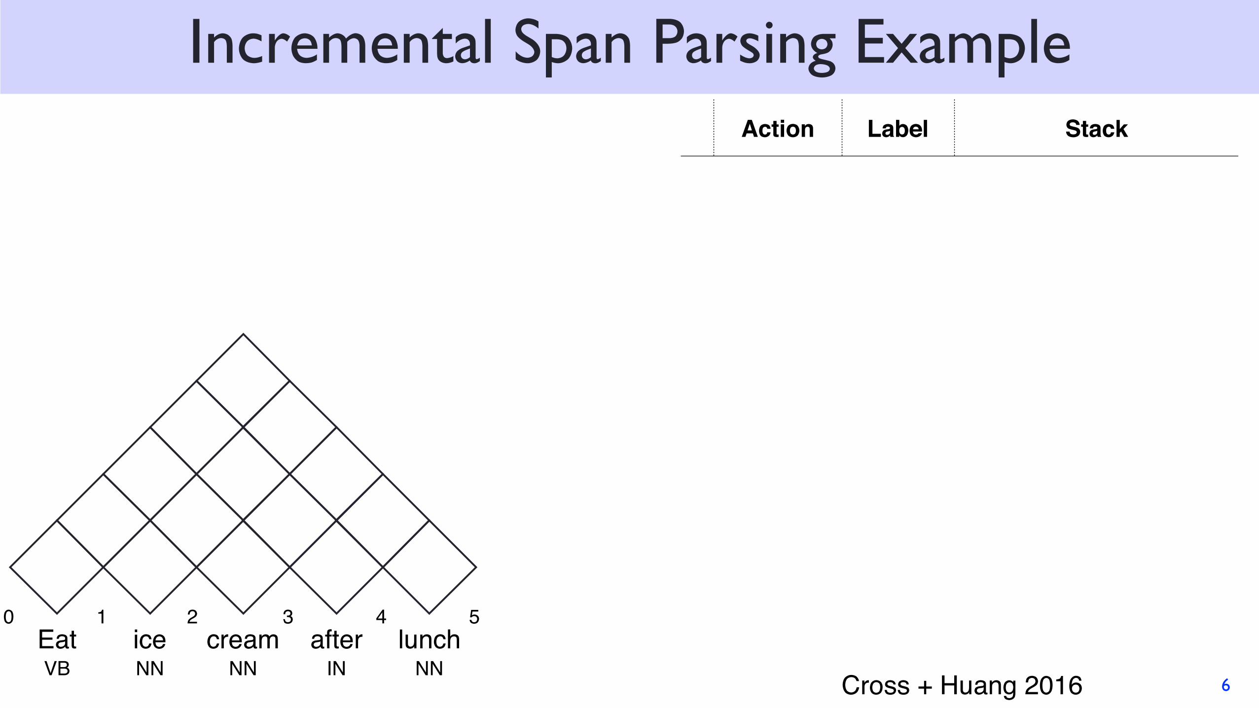
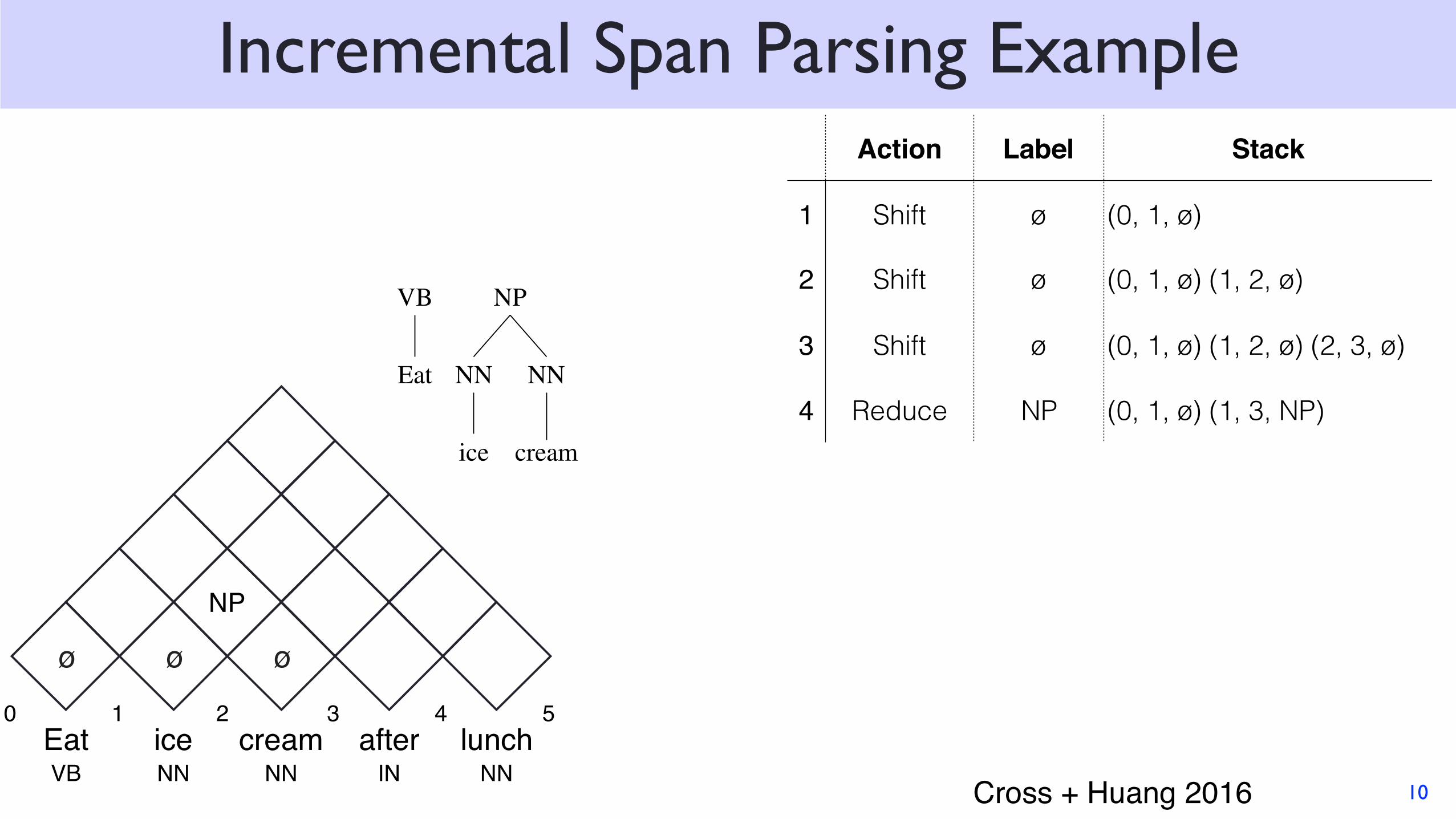
Incremental Span Parsing Example
6
EatVB
1ice NN
creamNN
afterIN
lunch NN
2 3 4 50
Action Label Stack
Cross + Huang 2016

S
VP
PP
NP
NN
lunch
IN
after
NP
NN
cream
NN
ice
VB
Eat
Incremental Span Parsing Example
7
EatVB
1ice NN
creamNN
afterIN
lunch NN
2 3 4 50
ø
Action Label Stack
1 Shift ø (0, 1, ø)
Cross + Huang 2016
S
VP
PP
NP
NN
lunch
IN
after
NP
NN
cream
NN
ice
VB
Eat
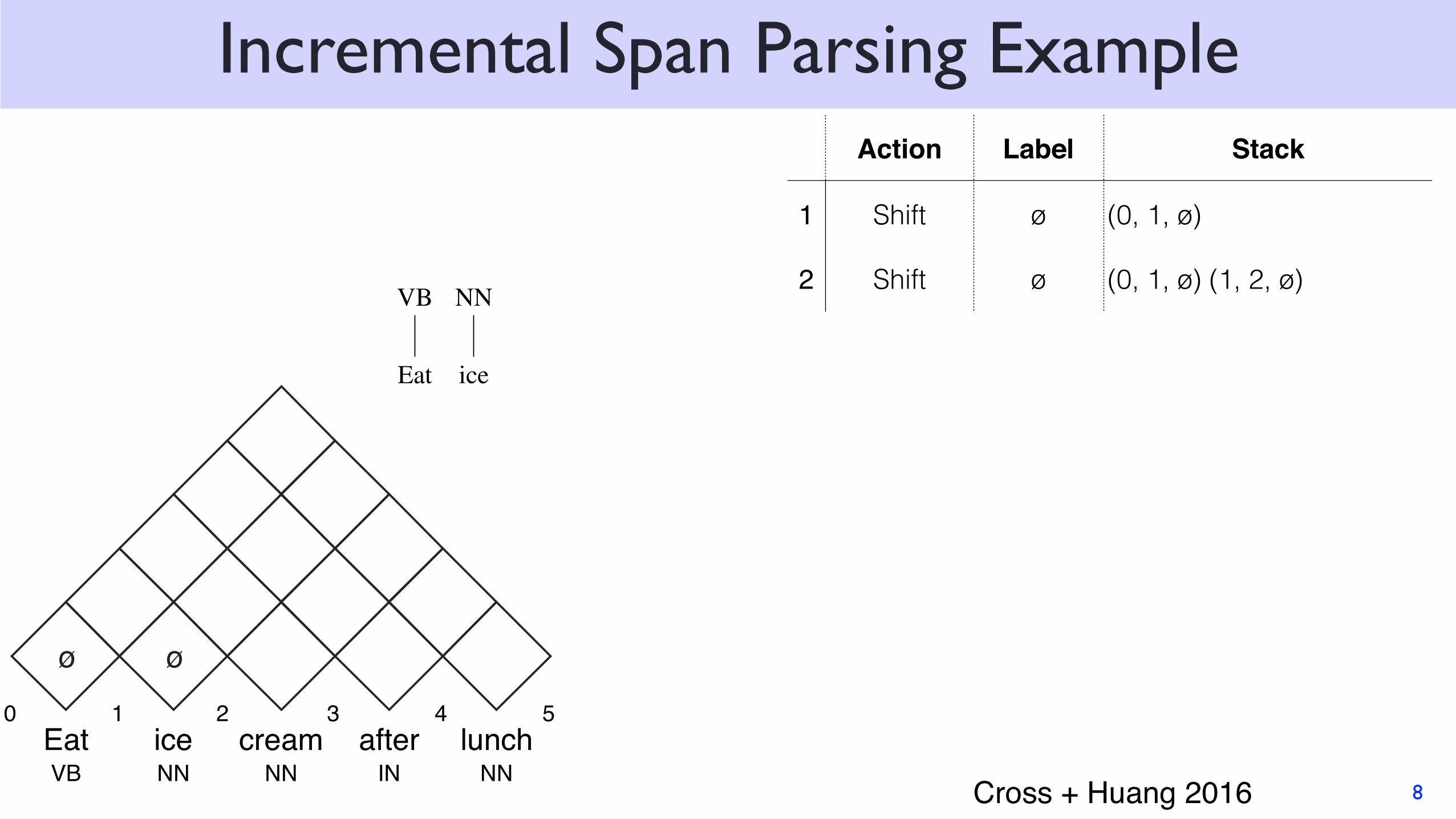
Incremental Span Parsing Example
8
EatVB
1ice NN
creamNN
afterIN
lunch NN
2 3 4 50
ø ø
Action Label Stack
1 Shift ø (0, 1, ø)
2 Shift ø (0, 1, ø) (1, 2, ø)
Cross + Huang 2016
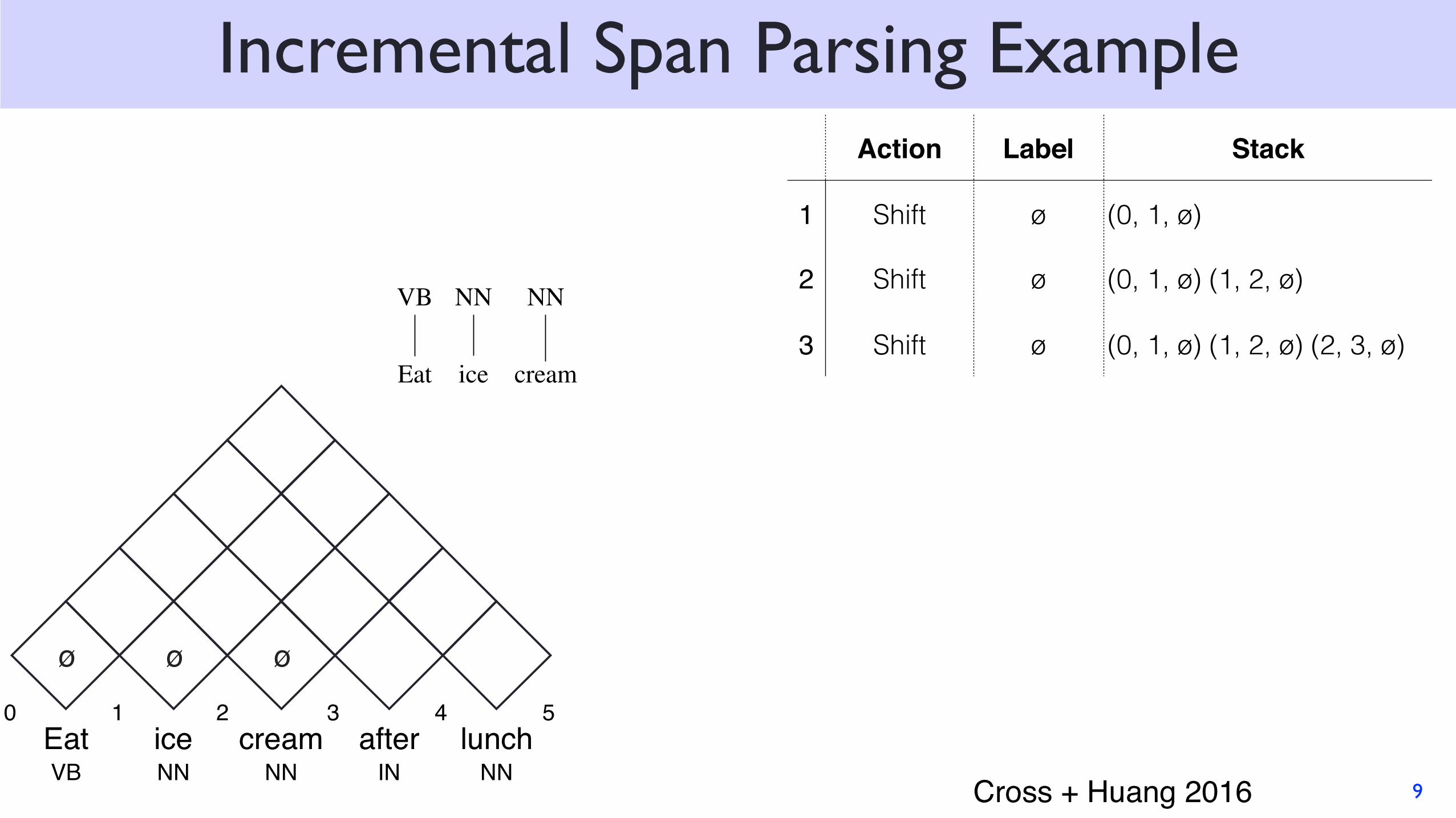
Incremental Span Parsing Example
9
EatVB
1ice NN
creamNN
afterIN
lunch NN
2 3 4 50
ø ø ø
S
PP
NP
NN
lunch
IN
after
VP
NP
NN
cream
NN
cream
NN
ice
VB
Eat
Action Label Stack
1 Shift ø (0, 1, ø)
2 Shift ø (0, 1, ø) (1, 2, ø)
3 Shift ø (0, 1, ø) (1, 2, ø) (2, 3, ø)
Cross + Huang 2016
S
VP
PP
NP
NN
lunch
IN
after
NP
NN
cream
NN
ice
VB
Eat
Incremental Span Parsing Example
10
EatVB
1ice NN
creamNN
afterIN
lunch NN
2 3 4 50
ø ø
NP
ø
Action Label Stack
1 Shift ø (0, 1, ø)
2 Shift ø (0, 1, ø) (1, 2, ø)
3 Shift ø (0, 1, ø) (1, 2, ø) (2, 3, ø)
4 Reduce NP (0, 1, ø) (1, 3, NP)
Cross + Huang 2016
S
temp
PP
NP
NN
lunch
IN
after
?
NP
NN
cream
NN
ice
VB
Eat
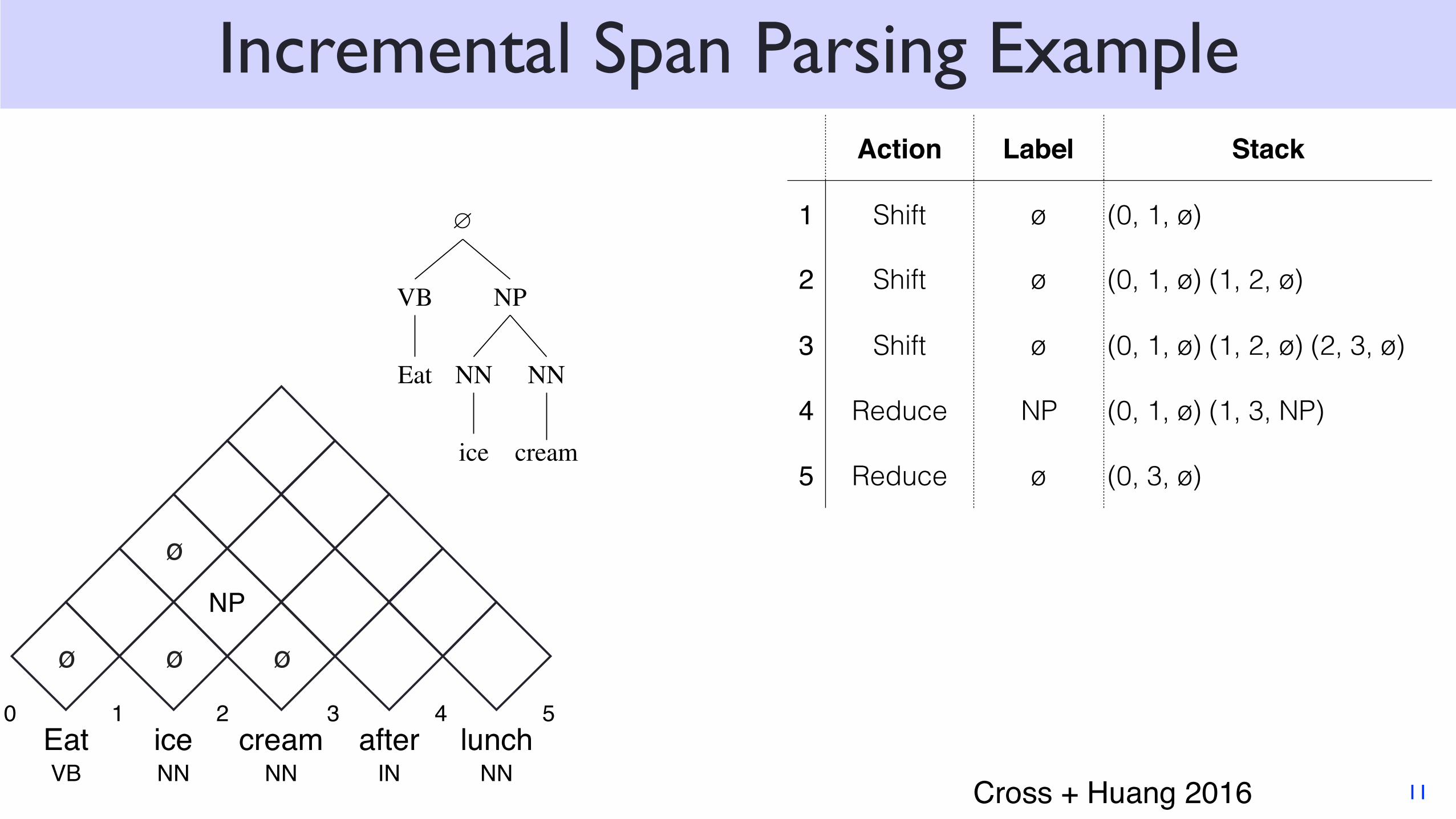
Incremental Span Parsing Example
11
EatVB
1ice NN
creamNN
afterIN
lunch NN
2 3 4 50
ø ø
øNP
ø
Action Label Stack
1 Shift ø (0, 1, ø)
2 Shift ø (0, 1, ø) (1, 2, ø)
3 Shift ø (0, 1, ø) (1, 2, ø) (2, 3, ø)
4 Reduce NP (0, 1, ø) (1, 3, NP)
5 Reduce ø (0, 3, ø)
Cross + Huang 2016
S
temp
PP
NP
NN
lunch
IN
after
?
NP
NN
cream
NN
ice
VB
Eat
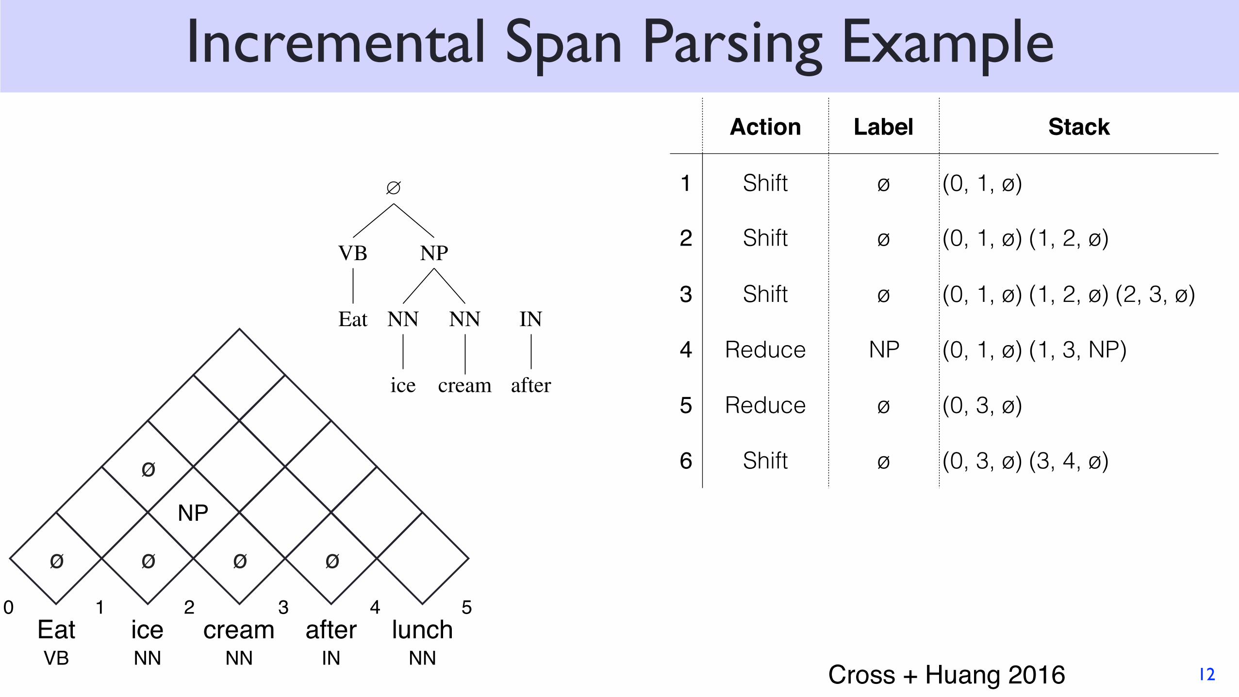
Incremental Span Parsing Example
12
EatVB
1ice NN
creamNN
afterIN
lunch NN
2 3 4 50
ø ø
øNP
ø ø
Action Label Stack
1 Shift ø (0, 1, ø)
2 Shift ø (0, 1, ø) (1, 2, ø)
3 Shift ø (0, 1, ø) (1, 2, ø) (2, 3, ø)
4 Reduce NP (0, 1, ø) (1, 3, NP)
5 Reduce ø (0, 3, ø)
6 Shift ø (0, 3, ø) (3, 4, ø)
Cross + Huang 2016
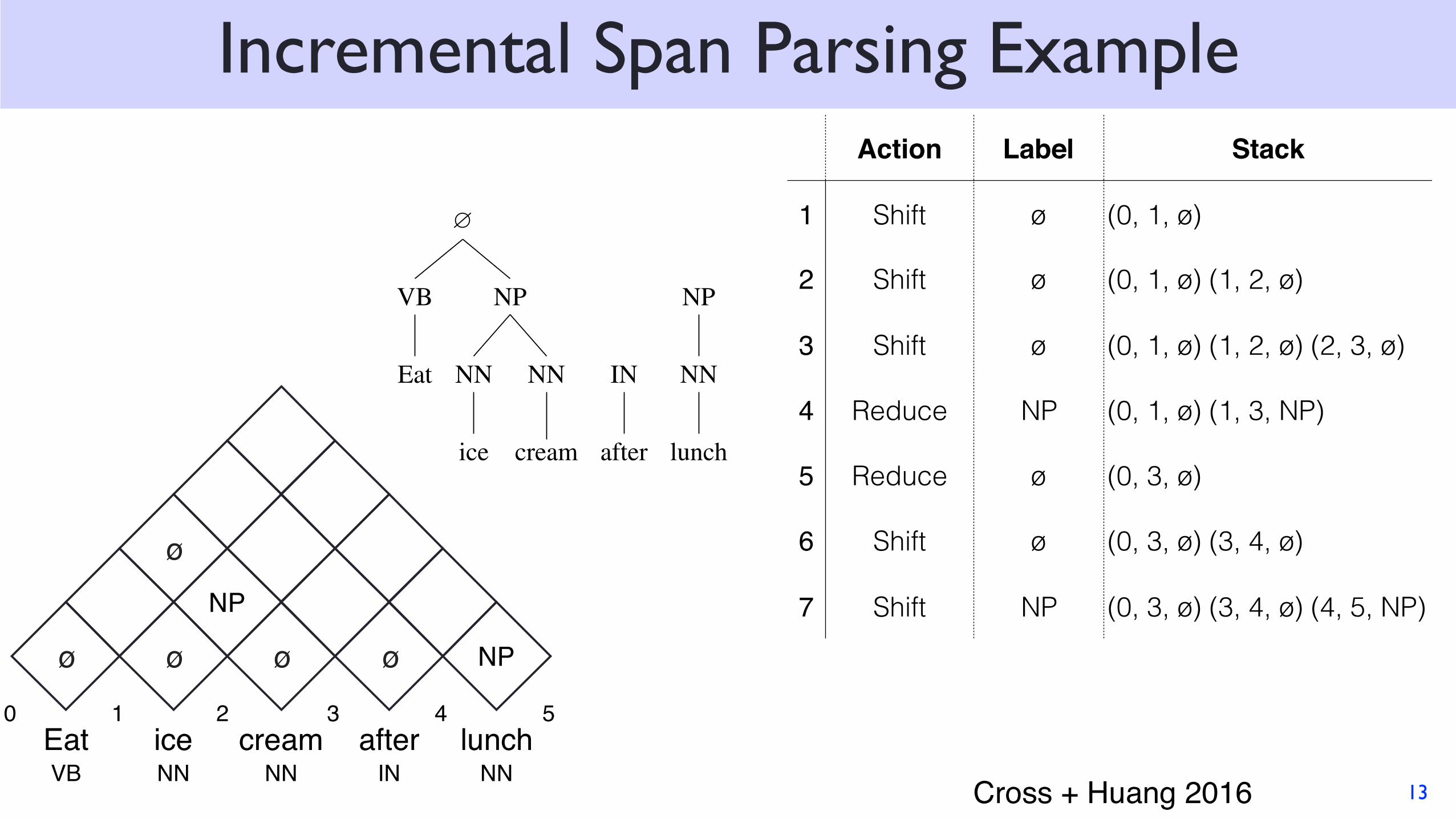
Incremental Span Parsing Example
13
EatVB
1ice NN
creamNN
afterIN
lunch NN
2 3 4 50
ø ø
øNP
ø ø NP
S
temp
NP
NN
lunch
PP
IN
after
?
NP
NN
cream
NN
ice
VB
Eat
Action Label Stack
1 Shift ø (0, 1, ø)
2 Shift ø (0, 1, ø) (1, 2, ø)
3 Shift ø (0, 1, ø) (1, 2, ø) (2, 3, ø)
4 Reduce NP (0, 1, ø) (1, 3, NP)
5 Reduce ø (0, 3, ø)
6 Shift ø (0, 3, ø) (3, 4, ø)
7 Shift NP (0, 3, ø) (3, 4, ø) (4, 5, NP)
Cross + Huang 2016

Incremental Span Parsing Example
14
EatVB
1ice NN
creamNN
afterIN
lunch NN
2 3 4 50
ø ø
øNP
ø ø
PP
NP
S
temp
PP
NP
NN
lunch
IN
after
?
NP
NN
cream
NN
ice
VB
Eat
Action Label Stack
1 Shift ø (0, 1, ø)
2 Shift ø (0, 1, ø) (1, 2, ø)
3 Shift ø (0, 1, ø) (1, 2, ø) (2, 3, ø)
4 Reduce NP (0, 1, ø) (1, 3, NP)
5 Reduce ø (0, 3, ø)
6 Shift ø (0, 3, ø) (3, 4, ø)
7 Shift NP (0, 3, ø) (3, 4, ø) (4, 5, NP)
8 Reduce PP (0, 3, ø) (3, 5, PP)
Cross + Huang 2016
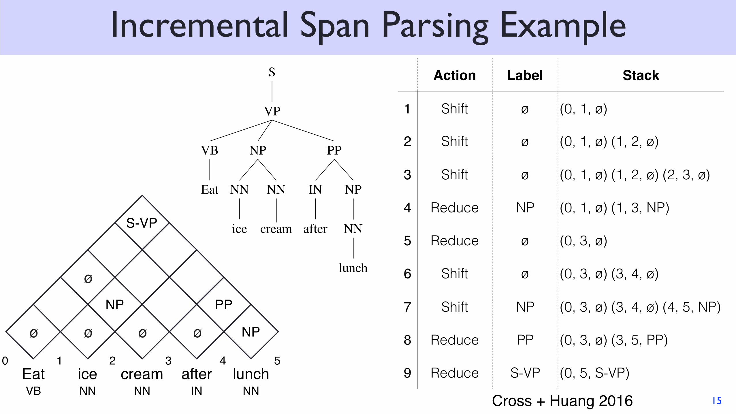
Incremental Span Parsing Example
15
EatVB
1ice NN
creamNN
afterIN
lunch NN
2 3 4 50
S
VP
PP
NP
NN
lunch
IN
after
NP
NN
cream
NN
ice
VB
Eat
Action Label Stack
1 Shift ø (0, 1, ø)
2 Shift ø (0, 1, ø) (1, 2, ø)
3 Shift ø (0, 1, ø) (1, 2, ø) (2, 3, ø)
4 Reduce NP (0, 1, ø) (1, 3, NP)
5 Reduce ø (0, 3, ø)
6 Shift ø (0, 3, ø) (3, 4, ø)
7 Shift NP (0, 3, ø) (3, 4, ø) (4, 5, NP)
8 Reduce PP (0, 3, ø) (3, 5, PP)
9 Reduce S-VP (0, 5, S-VP)
ø ø
øNP
ø ø
PP
NP
S-VP
Cross + Huang 2016

16
O(3n)
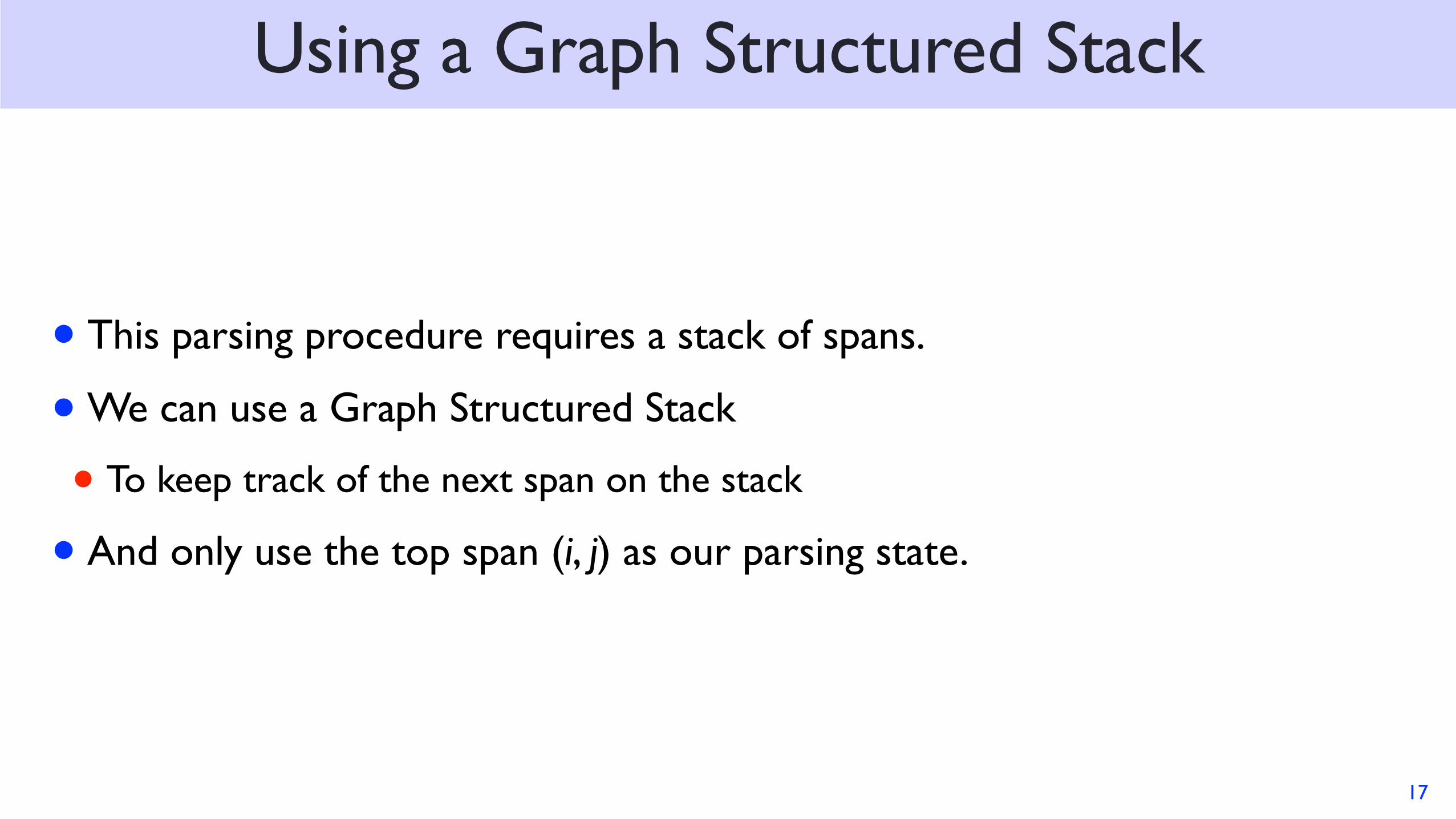
Using a Graph Structured Stack
• This parsing procedure requires a stack of spans.
• We can use a Graph Structured Stack
• To keep track of the next span on the stack
• And only use the top span (i, j) as our parsing state.
17
1
✏ (0,1) (1,2) (2,3) (3,4) (4,5) (3,5) (2,5) (1,5) (0,5)
(0,2) (1,3) (2,4) (4,5) (3,5) (2,5)
(2,3) (3,4) (1,4) (4,5) (3,5)
(0,3) (2,4) (0,4) (4,5)
(3,4)
sh
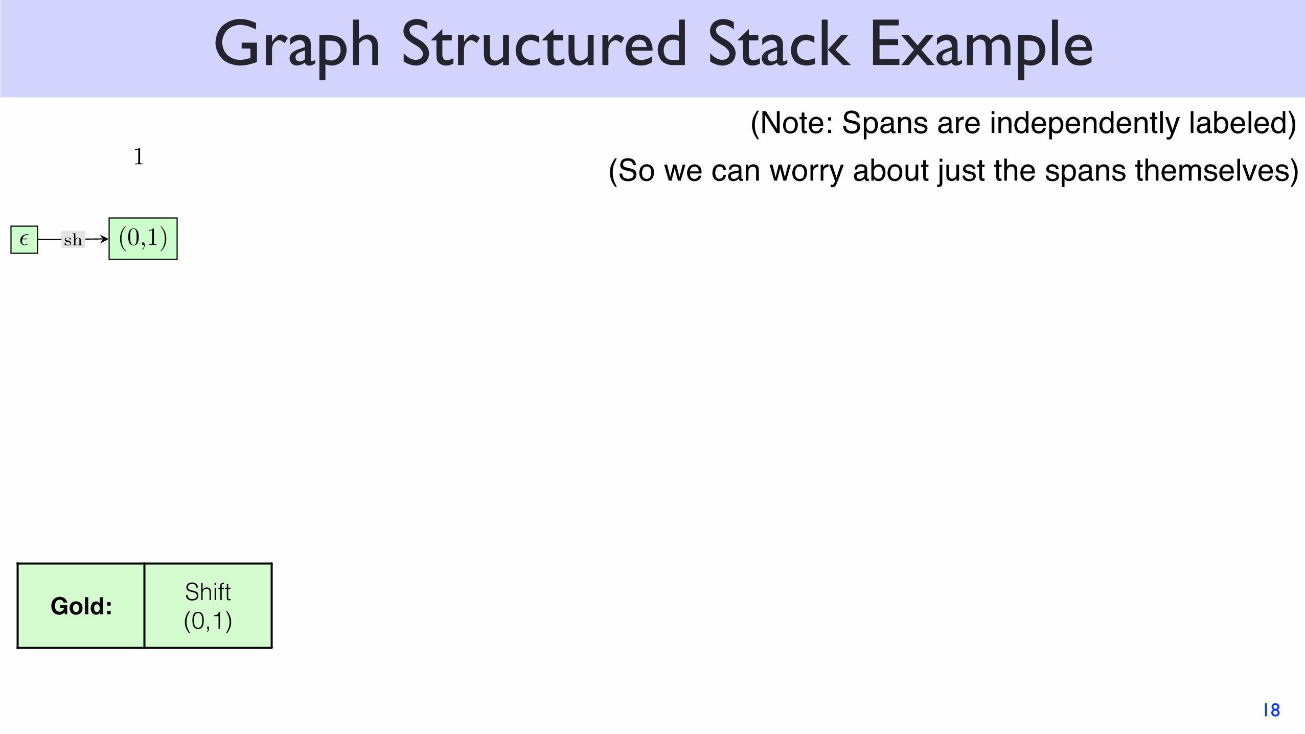
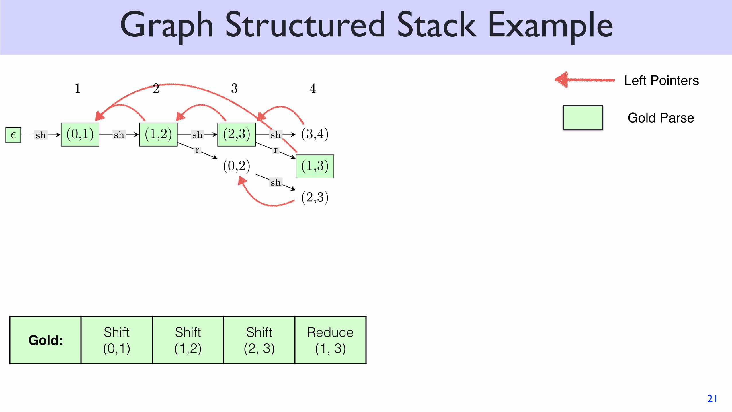
Graph Structured Stack Example
18
Gold: Shift (0,1)
(Note: Spans are independently labeled)(So we can worry about just the spans themselves)
1 2
✏ (0,1) (1,2) (2,3) (3,4) (4,5) (3,5) (2,5) (1,5) (0,5)
(0,2) (1,3) (2,4) (4,5) (3,5) (2,5)
(2,3) (3,4) (1,4) (4,5) (3,5)
(0,3) (2,4) (0,4) (4,5)
(3,4)
sh sh
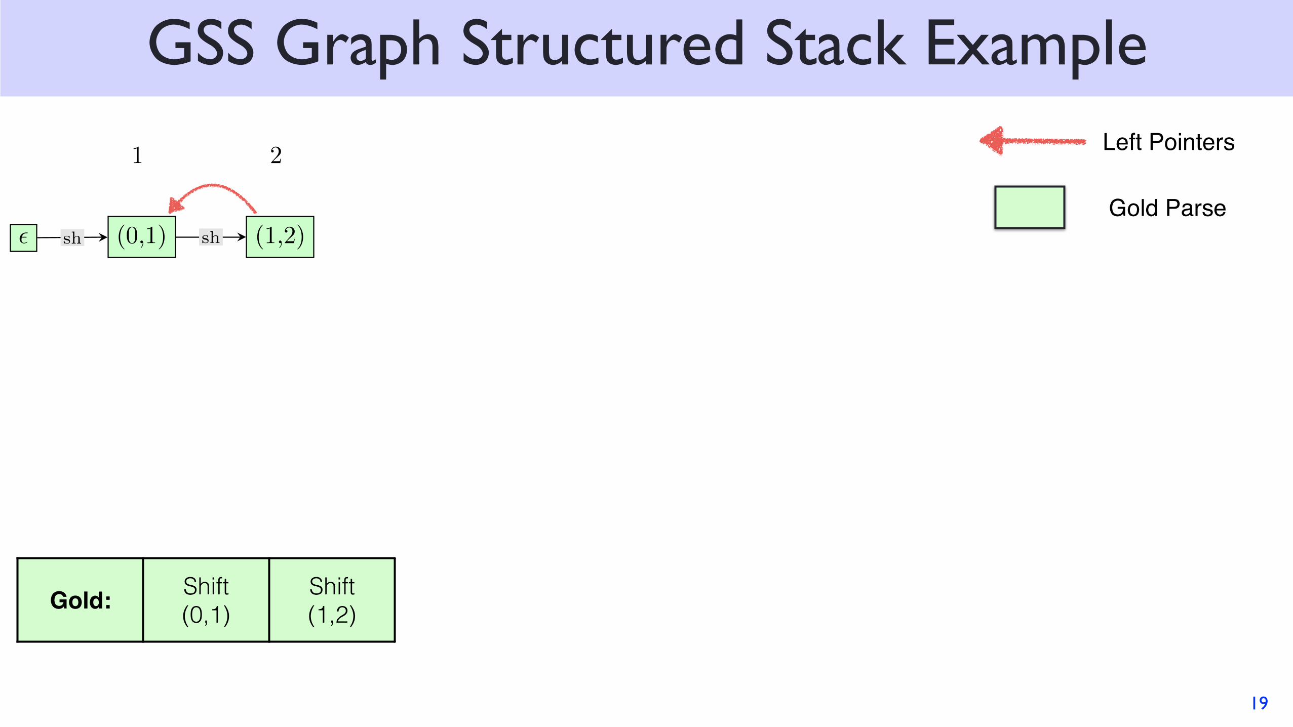
GSS Graph Structured Stack Example
19
Gold: Shift (0,1)
Shift (1,2)
Left Pointers
Gold Parse

1 2 3
✏ (0,1) (1,2) (2,3) (3,4) (4,5) (3,5) (2,5) (1,5) (0,5)
(0,2) (1,3) (2,4) (4,5) (3,5) (2,5)
(2,3) (3,4) (1,4) (4,5) (3,5)
(0,3) (2,4) (0,4) (4,5)
(3,4)
sh sh sh
r
Graph Structured Stack Example
20
Gold: Shift (0,1)
Shift (1,2)
Shift (2, 3)
Left Pointers
Gold Parse
Graph Structured Stack Example
21
Gold: Shift (0,1)
Shift (1,2)
Shift (2, 3)
Reduce (1, 3)
Left Pointers1 2 3 4
✏ (0,1) (1,2) (2,3) (3,4) (4,5) (3,5) (2,5) (1,5) (0,5)
(0,2) (1,3) (2,4) (4,5) (3,5) (2,5)
(2,3) (3,4) (1,4) (4,5) (3,5)
(0,3) (2,4) (0,4) (4,5)
(3,4)
sh sh sh
r
sh
r
sh
Gold Parse
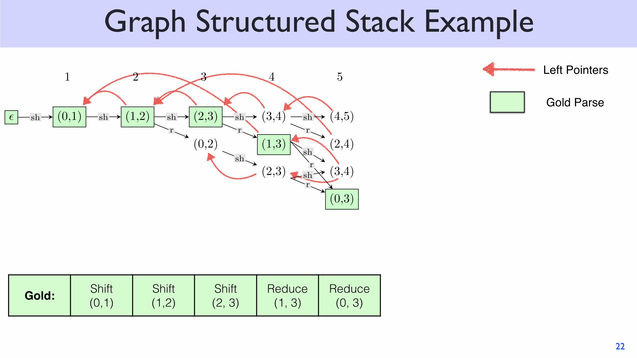
Graph Structured Stack Example
22
Gold: Shift (0,1)
Shift (1,2)
Shift (2, 3)
Reduce (1, 3)
Reduce (0, 3)
Left Pointers1 2 3 4 5
✏ (0,1) (1,2) (2,3) (3,4) (4,5) (3,5) (2,5) (1,5) (0,5)
(0,2) (1,3) (2,4) (4,5) (3,5) (2,5)
(2,3) (3,4) (1,4) (4,5) (3,5)
(0,3) (2,4) (0,4) (4,5)
(3,4)
sh sh sh
r
sh
r
sh
sh
r
sh
rshr
Gold Parse
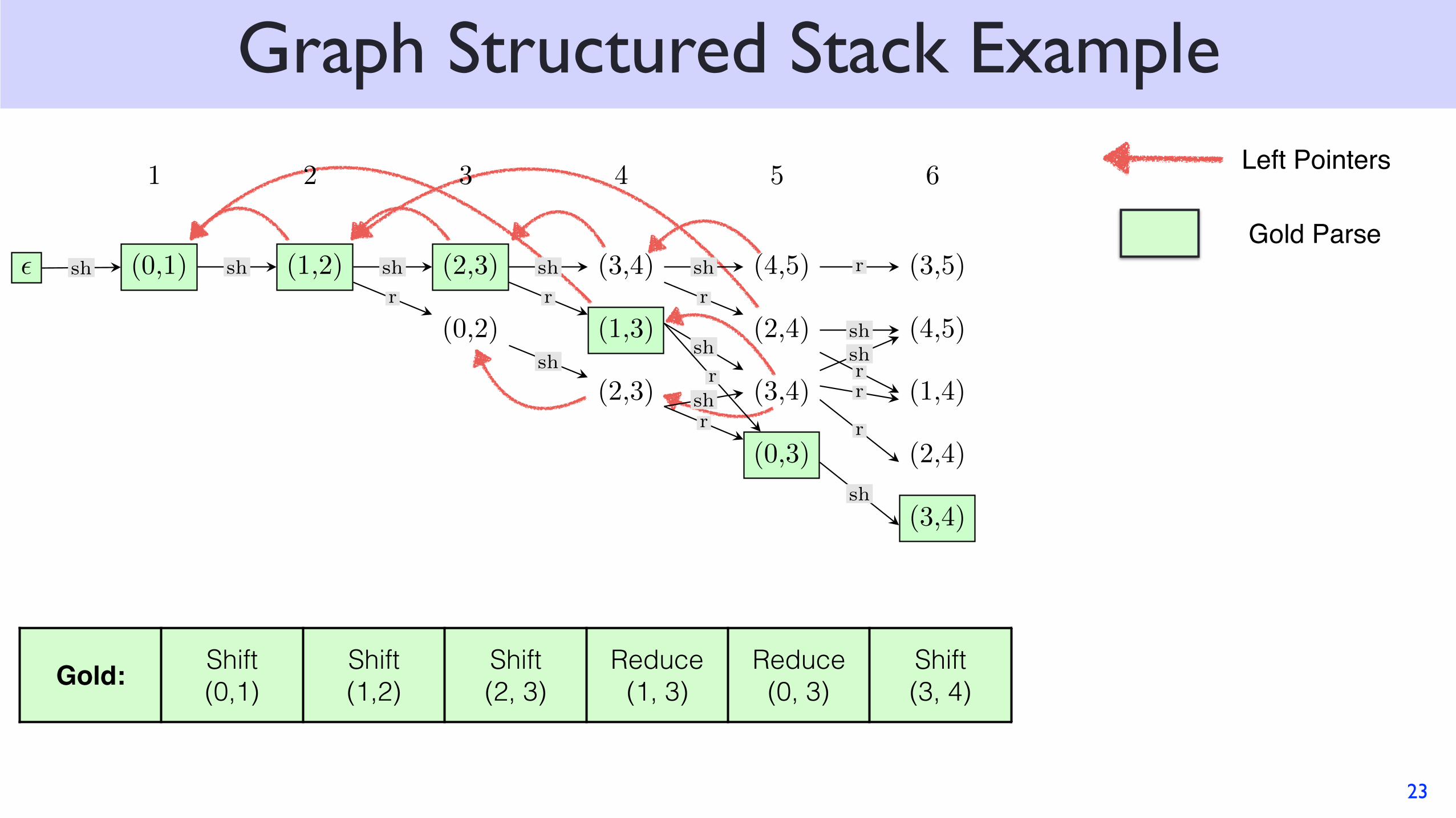
Graph Structured Stack Example
23
Gold: Shift (0,1)
Shift (1,2)
Shift (2, 3)
Reduce (1, 3)
Reduce (0, 3)
Shift (3, 4)
Left Pointers
Gold Parse
1 2 3 4 5 6
✏ (0,1) (1,2) (2,3) (3,4) (4,5) (3,5) (2,5) (1,5) (0,5)
(0,2) (1,3) (2,4) (4,5) (3,5) (2,5)
(2,3) (3,4) (1,4) (4,5) (3,5)
(0,3) (2,4) (0,4) (4,5)
(3,4)
sh sh sh
r
sh
r
sh
sh
r
sh
rshr
r
sh
rsh
r
r
sh

1 2 3 4 5 6 7 8 9
✏ (0,1) (1,2) (2,3) (3,4) (4,5) (3,5) (2,5) (1,5) (0,5)
(0,2) (1,3) (2,4) (4,5) (3,5) (2,5)
(2,3) (3,4) (1,4) (4,5) (3,5)
(0,3) (2,4) (0,4) (4,5)
(3,4)
sh sh sh
r
sh
r
sh
sh
r
sh
rshr
r
sh
rsh
r
r
sh
r
r
r
sh
r
rsh
r
r
r
rr
r
sh
r
r
r
r
Graph Structured Stack Example
24
Gold: Shift (0,1)
Shift (1,2)
Shift (2, 3)
Reduce (1, 3)
Reduce (0, 3)
Shift (3, 4)
Shift (4, 5)
Reduce (3, 5)
Reduce (0, 5)
1 2 3 4 5 6 7 8 9
✏ (0,1) (1,2) (2,3) (3,4) (4,5) (3,5) (2,5) (1,5) (0,5)
(0,2) (1,3) (2,4) (4,5) (3,5) (2,5)
(2,3) (3,4) (1,4) (4,5) (3,5)
(0,3) (2,4) (0,4) (4,5)
(3,4)
sh sh sh
r
sh
r
sh
sh
r
sh
rshr
r
sh
rsh
r
r
sh
r
r
r
sh
r
rsh
r
r
r
rr
r
sh
r
r
r
r
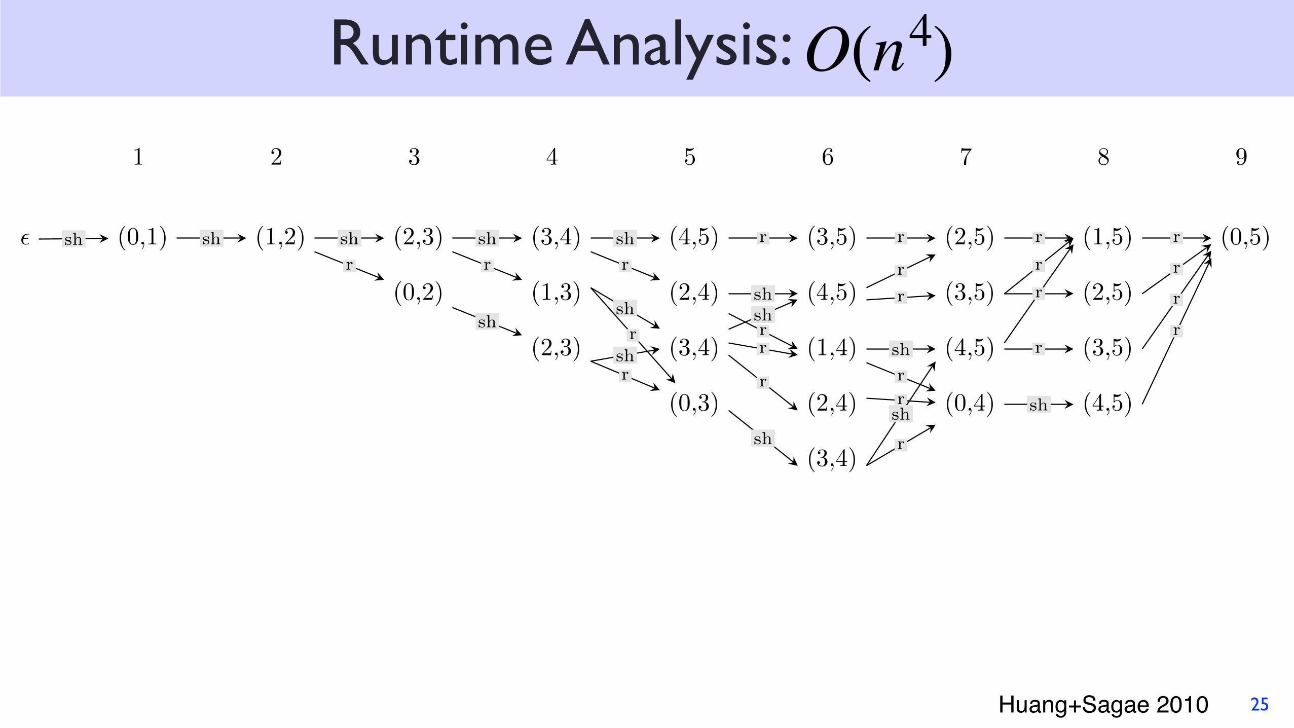
Runtime Analysis: .
25
O(n4)
Huang+Sagae 2010
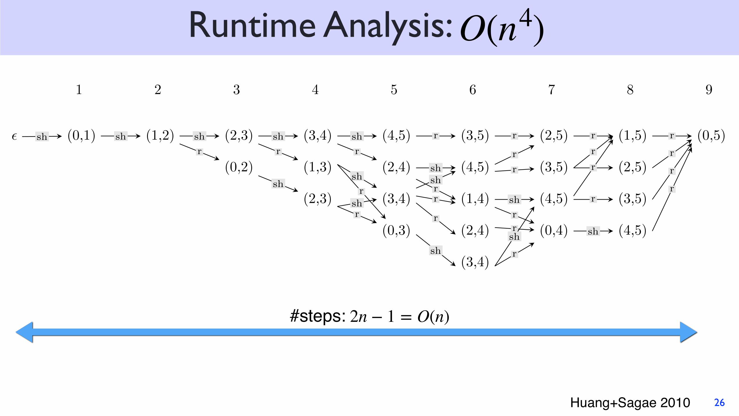
Runtime Analysis: .
26
O(n4)
#steps: 2n − 1 = O(n)
1 2 3 4 5 6 7 8 9
✏ (0,1) (1,2) (2,3) (3,4) (4,5) (3,5) (2,5) (1,5) (0,5)
(0,2) (1,3) (2,4) (4,5) (3,5) (2,5)
(2,3) (3,4) (1,4) (4,5) (3,5)
(0,3) (2,4) (0,4) (4,5)
(3,4)
sh sh sh
r
sh
r
sh
sh
r
sh
rshr
r
sh
rsh
r
r
sh
r
r
r
sh
r
rsh
r
r
r
rr
r
sh
r
r
r
r
Huang+Sagae 2010
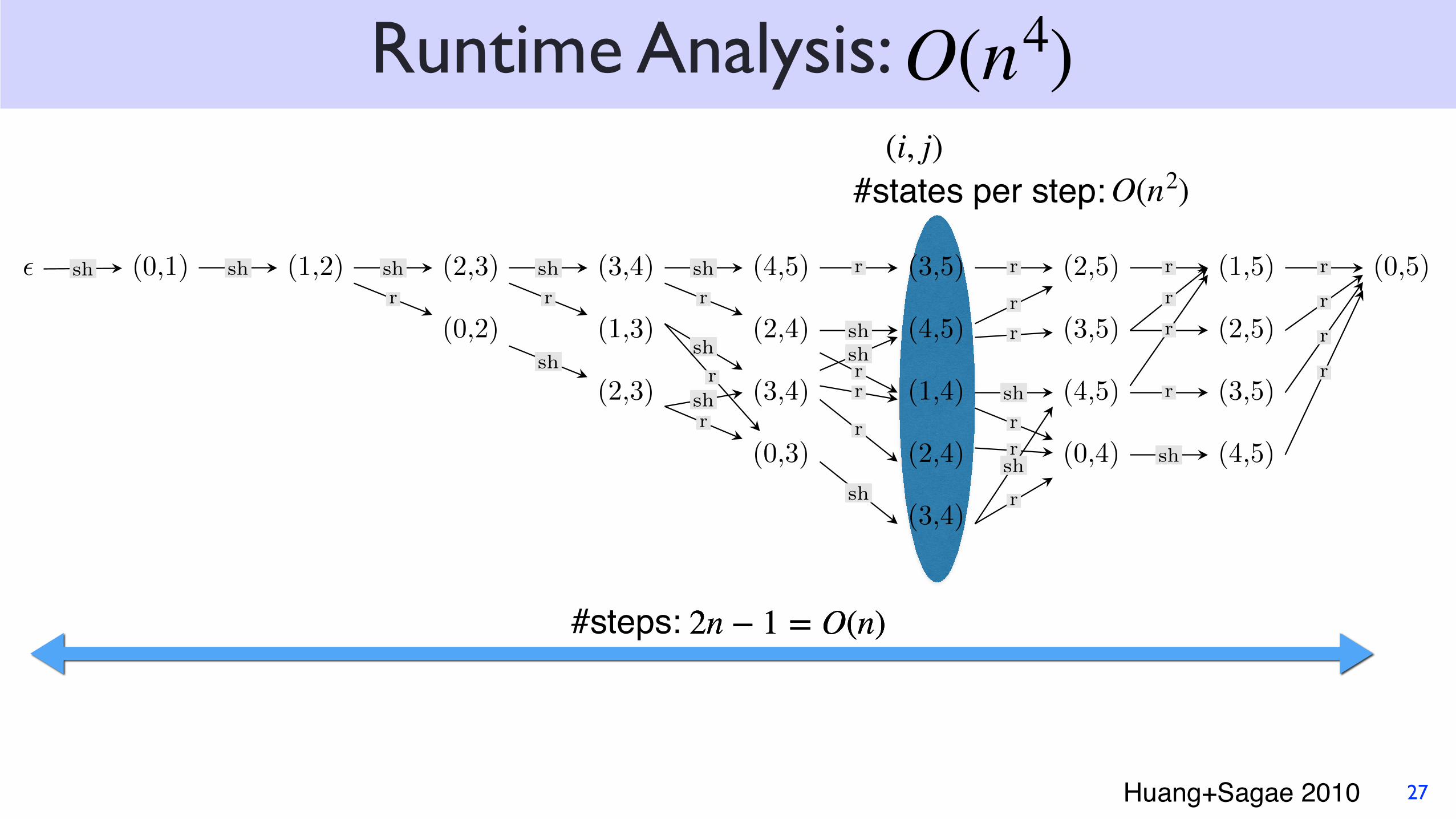
Runtime Analysis: .
27
O(n4)O(n2)#states per step:
(i, j)
2n − 1 = O(n)2n − 1 = O(n)2n − 1 = O(n)#steps:
1 2 3 4 5 6 7 8 9
✏ (0,1) (1,2) (2,3) (3,4) (4,5) (3,5) (2,5) (1,5) (0,5)
(0,2) (1,3) (2,4) (4,5) (3,5) (2,5)
(2,3) (3,4) (1,4) (4,5) (3,5)
(0,3) (2,4) (0,4) (4,5)
(3,4)
sh sh sh
r
sh
r
sh
sh
r
sh
rshr
r
sh
rsh
r
r
sh
r
r
r
sh
r
rsh
r
r
r
rr
r
sh
r
r
r
r
Huang+Sagae 2010
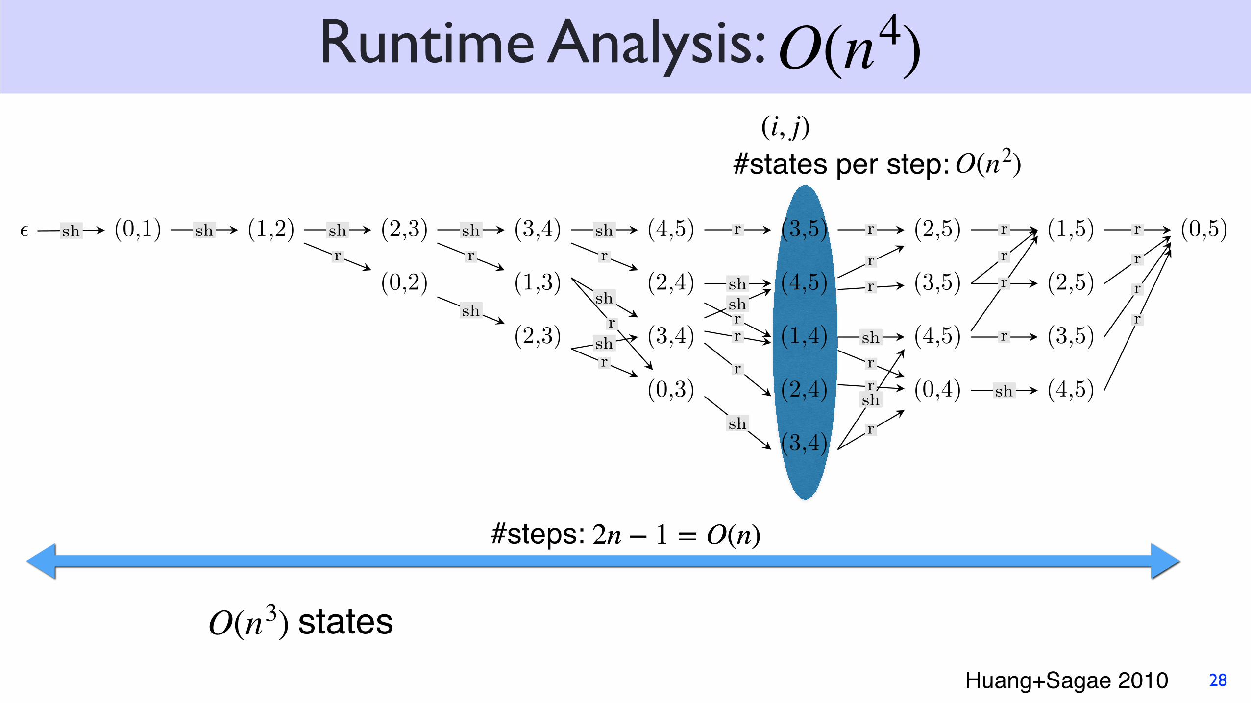
Runtime Analysis: .
28
O(n4)(i, j)
2n − 1 = O(n)2n − 1 = O(n)#steps:
O(n2)#states per step:
statesO(n3)
1 2 3 4 5 6 7 8 9
✏ (0,1) (1,2) (2,3) (3,4) (4,5) (3,5) (2,5) (1,5) (0,5)
(0,2) (1,3) (2,4) (4,5) (3,5) (2,5)
(2,3) (3,4) (1,4) (4,5) (3,5)
(0,3) (2,4) (0,4) (4,5)
(3,4)
sh sh sh
r
sh
r
sh
sh
r
sh
rshr
r
sh
rsh
r
r
sh
r
r
r
sh
r
rsh
r
r
r
rr
r
sh
r
r
r
r
Huang+Sagae 2010

✏ (0,1) (1,2) (2,3) (3,4) (4,5) (3,5) (2,5) (1,5) (0,5)
(0,2) (1,3) (2,4) (4,5) (3,5) (2,5)
(2,3) (3,4) (1,4) (4,5) (3,5)
(0,3) (2,4) (0,4) (4,5)
(3,4)
sh sh sh
r
sh
r
sh
sh
r
sh
rshr
r
sh
rsh
r
r
sh
r
r
r
sh
r
rsh
r
r
r
rr
r
sh
r
r
r
r
statesO(n3)
Runtime Analysis: .
29
O(n4)(i, j)
#left pointers per state: O(n)
2n − 1 = O(n)#steps:
O(n2)#states per step:
Check out the paper for Deng’s Theorem:
Huang+Sagae 2010
ℓ′ � = ℓ − 2( j − i) + 1

Runtime Analysis: .
30
O(n4)(i, j)
2n − 1 = O(n)
states with O(n3) O(n) reduce actions:
#steps:
O(n2)#states per step:
O(n4) runtime
✏ (0,1) (1,2) (2,3) (3,4) (4,5) (3,5) (2,5) (1,5) (0,5)
(0,2) (1,3) (2,4) (4,5) (3,5) (2,5)
(2,3) (3,4) (1,4) (4,5) (3,5)
(0,3) (2,4) (0,4) (4,5)
(3,4)
sh sh sh
r
sh
r
sh
sh
r
sh
rshr
r
sh
rsh
r
r
sh
r
r
r
sh
r
rsh
r
r
r
rr
r
sh
r
r
r
r
Huang+Sagae 2010
#left pointers per state: O(n)
Check out the paper for Deng’s Theorem:ℓ′ � = ℓ − 2( j − i) + 1

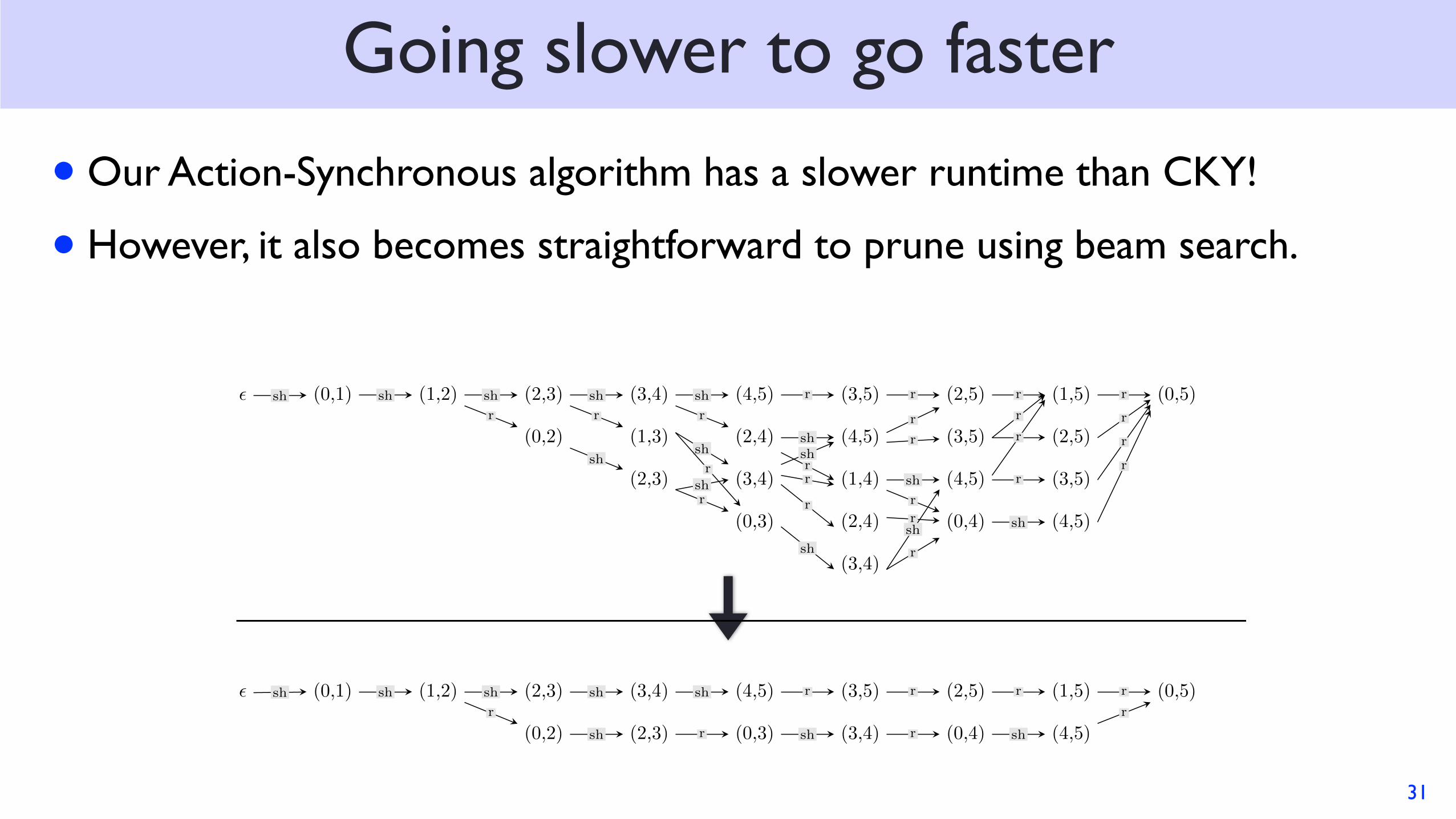
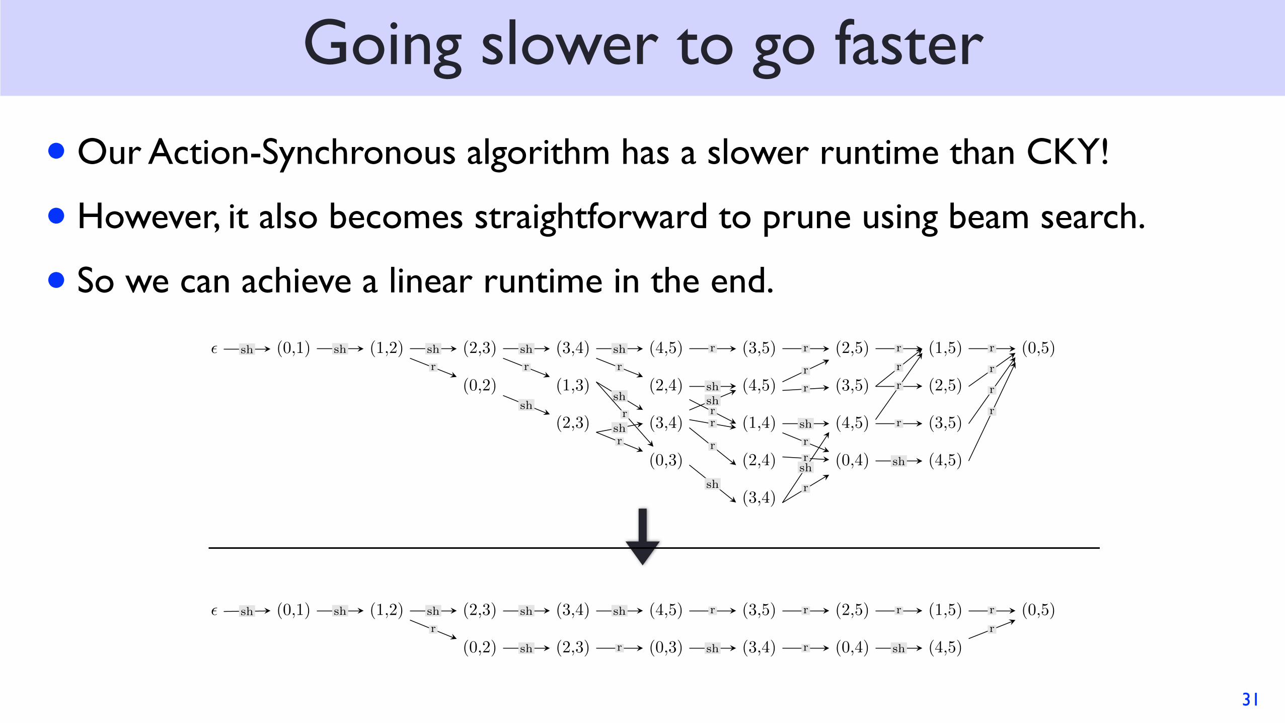
Going slower to go faster
• Our Action-Synchronous algorithm has a slower runtime than CKY!
31
DP+GSS
✏ (0,1) (1,2) (2,3) (3,4) (4,5) (3,5) (2,5) (1,5) (0,5) O(n4)
(0,2) (1,3) (2,4) (4,5) (3,5) (2,5)
(2,3) (3,4) (1,4) (4,5) (3,5)
(0,3) (2,4) (0,4) (4,5)
(3,4)
DP+GSS+Beam
✏ (0,1) (1,2) (2,3) (3,4) (4,5) (3,5) (2,5) (1,5) (0,5) O(n)
(0,2) (1,3) (2,4) (4,5) (4,5) (3,5) (approx. DP)
(2,3) (0,3) (3,4) (0,4) (4,5)
sh sh sh
r
sh
r
sh
sh
r
sh
rshr
r
sh
rsh
r
r
sh
r
r
r
sh
r
rsh
r
r
r
rr
r
sh
r
r
r
r
sh sh sh
r
sh
r
sh
sh
r
r
r
r
sh
sh
r
r
sh
r
r
r
sh
r
r
r
+beam
Going slower to go faster
• Our Action-Synchronous algorithm has a slower runtime than CKY!
• However, it also becomes straightforward to prune using beam search.
31
DP+GSS
✏ (0,1) (1,2) (2,3) (3,4) (4,5) (3,5) (2,5) (1,5) (0,5) O(n4)
(0,2) (1,3) (2,4) (4,5) (3,5) (2,5)
(2,3) (3,4) (1,4) (4,5) (3,5)
(0,3) (2,4) (0,4) (4,5)
(3,4)
DP+GSS+Beam
✏ (0,1) (1,2) (2,3) (3,4) (4,5) (3,5) (2,5) (1,5) (0,5) O(n)
(0,2) (2,3) (0,3) (3,4) (0,4) (4,5) (approx. DP)
sh sh sh
r
sh
r
sh
sh
r
sh
rshr
r
sh
rsh
r
r
sh
r
r
r
sh
r
rsh
r
r
r
rr
r
sh
r
r
r
r
sh sh sh
r
sh
sh
sh
r
r
sh
r
r
r
sh
r
r
+beam
Going slower to go faster
• Our Action-Synchronous algorithm has a slower runtime than CKY!
• However, it also becomes straightforward to prune using beam search.
• So we can achieve a linear runtime in the end.
31
DP+GSS
✏ (0,1) (1,2) (2,3) (3,4) (4,5) (3,5) (2,5) (1,5) (0,5) O(n4)
(0,2) (1,3) (2,4) (4,5) (3,5) (2,5)
(2,3) (3,4) (1,4) (4,5) (3,5)
(0,3) (2,4) (0,4) (4,5)
(3,4)
DP+GSS+Beam
✏ (0,1) (1,2) (2,3) (3,4) (4,5) (3,5) (2,5) (1,5) (0,5) O(n)
(0,2) (2,3) (0,3) (3,4) (0,4) (4,5) (approx. DP)
sh sh sh
r
sh
r
sh
sh
r
sh
rshr
r
sh
rsh
r
r
sh
r
r
r
sh
r
rsh
r
r
r
rr
r
sh
r
r
r
r
sh sh sh
r
sh
sh
sh
r
r
sh
r
r
r
sh
r
r
+beam
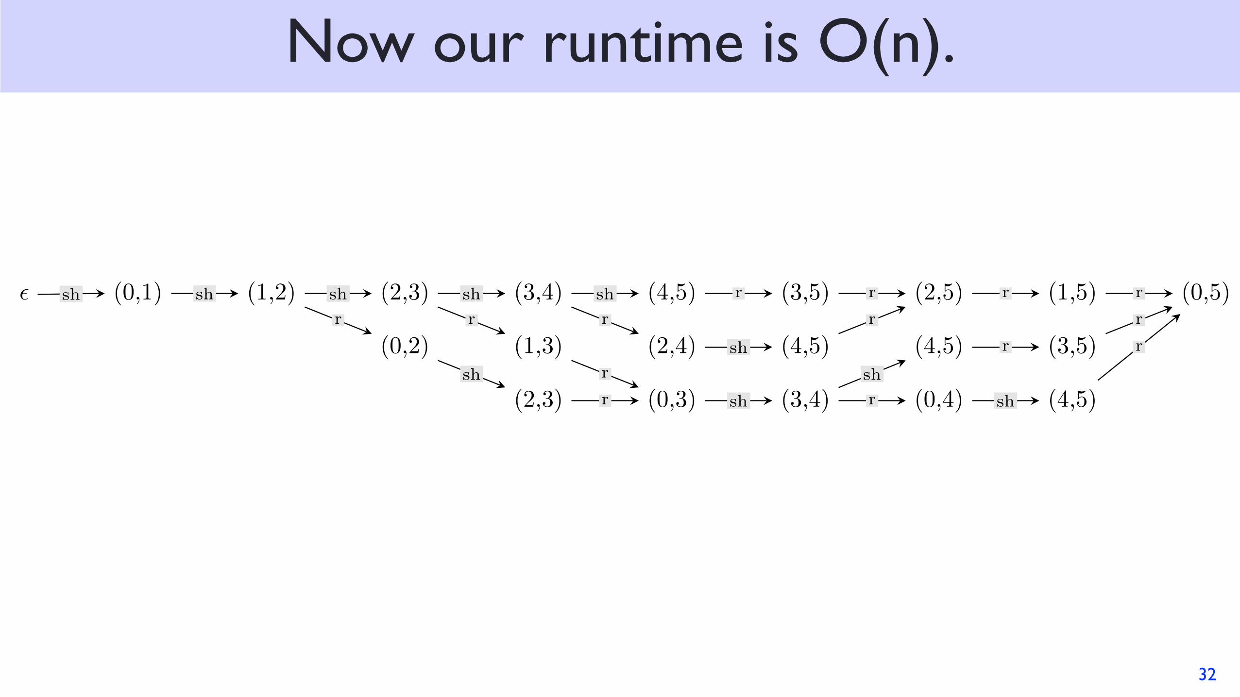
Now our runtime is O(n).
32
✏ (0,1) (1,2) (2,3) (3,4) (4,5) (3,5) (2,5) (1,5) (0,5)
(0,2) (1,3) (2,4) (4,5) (4,5) (3,5)
(2,3) (0,3) (3,4) (0,4) (4,5)
sh sh sh
r
sh
r
sh
sh
r
r
r
r
sh
sh
r
r
sh
r
r
r
sh
r
r
r

But the O(n) is hiding a constant.
33
✏ (0,1) (1,2) (2,3) (3,4) (4,5) (3,5)
(0,2) (1,3) (2,4) (4,5)
(2,3) (0,3) (3,4)
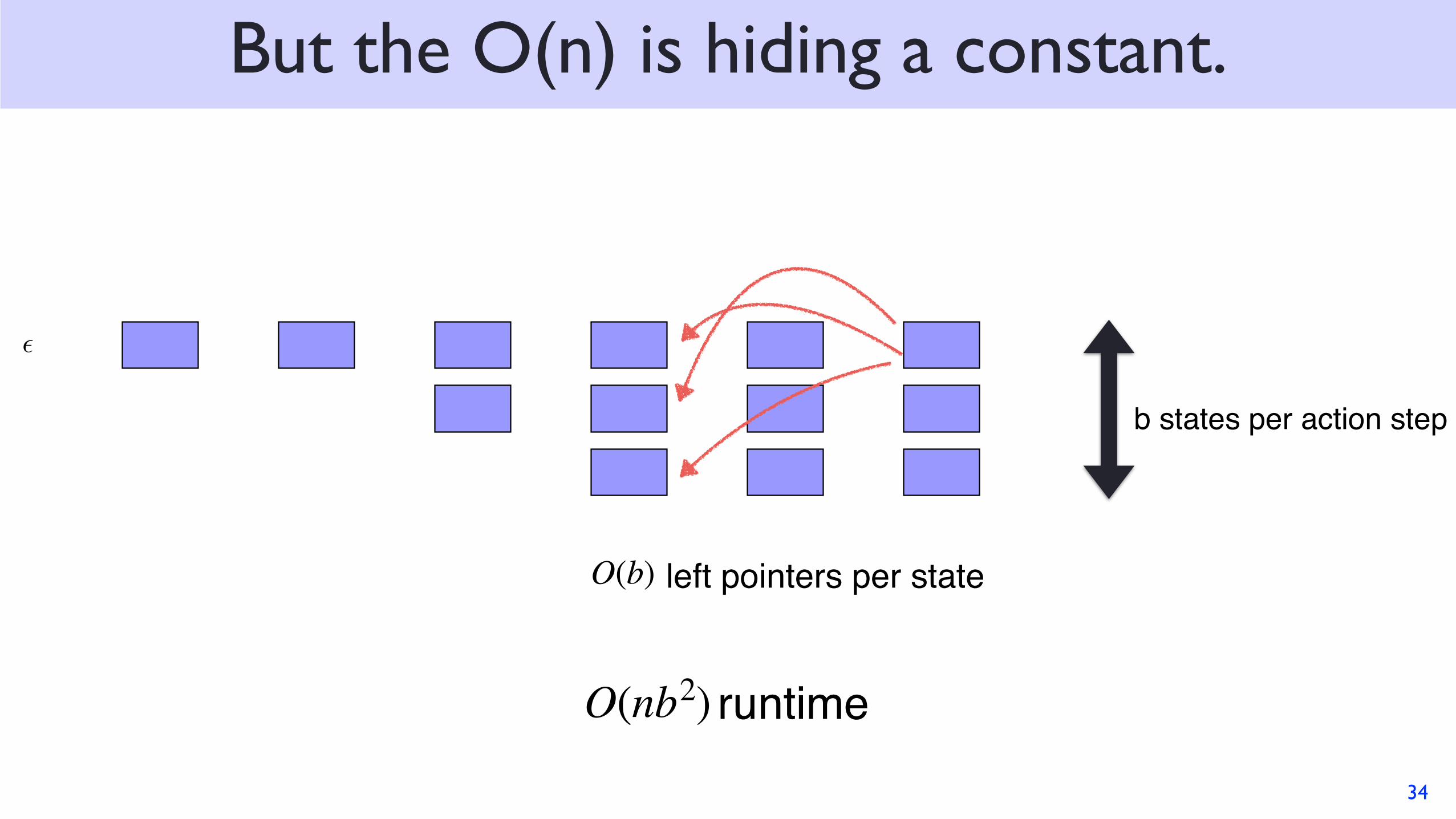
But the O(n) is hiding a constant.
34
O(b)
✏ (0,1) (1,2) (2,3) (3,4) (4,5) (3,5)
(0,2) (1,3) (2,4) (4,5)
(2,3) (0,3) (3,4)
left pointers per state
b states per action step
O(nb2) runtime
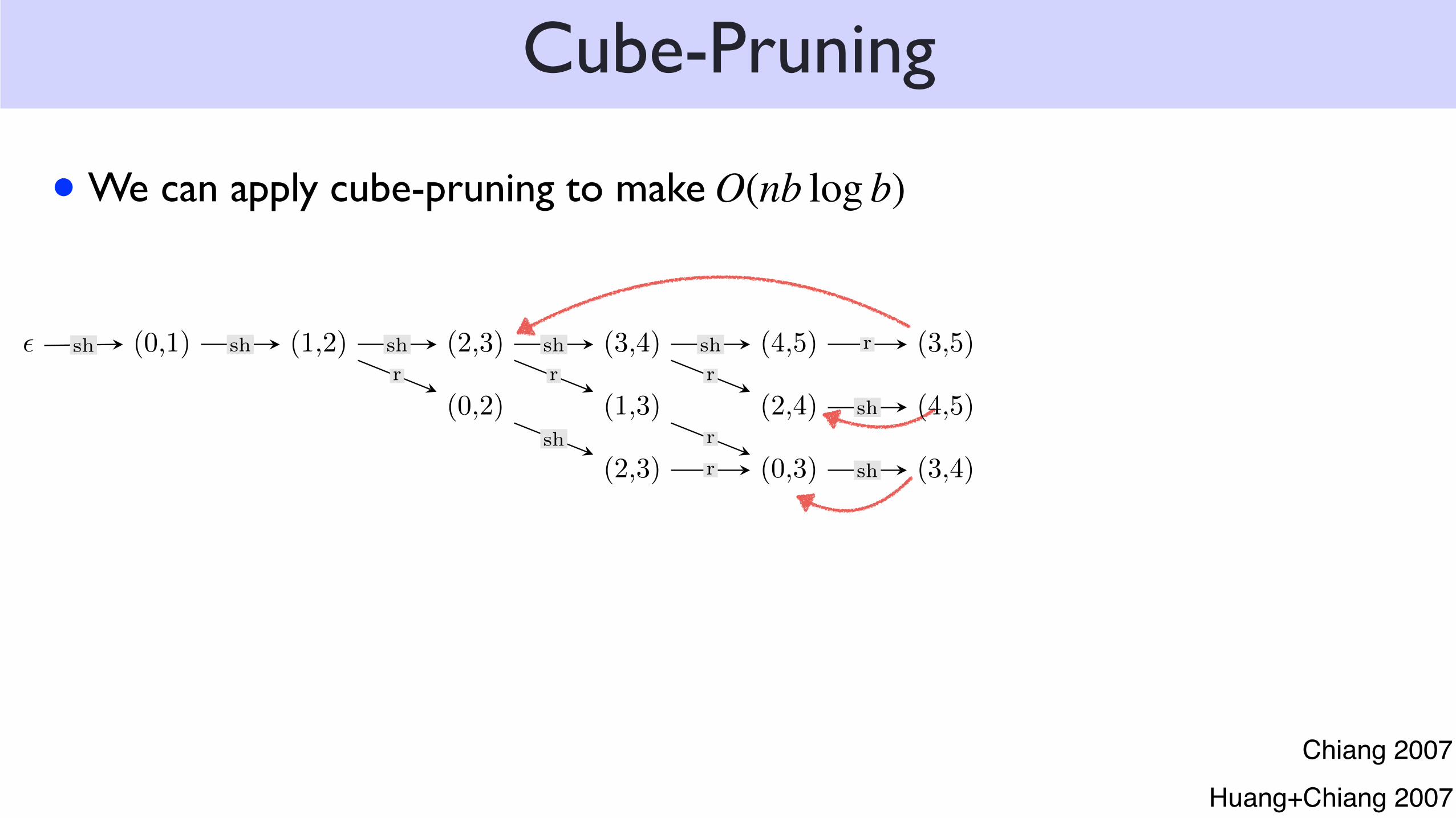
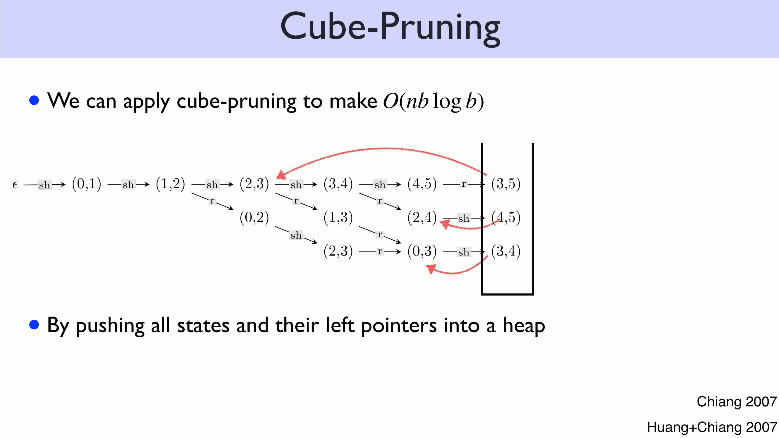
Cube-Pruning
• We can apply cube-pruning to make
✏ (0,1) (1,2) (2,3) (3,4) (4,5) (3,5) (2,5) (1,5) (0,5)
(0,2) (1,3) (2,4) (4,5) (4,5) (3,5)
(2,3) (0,3) (3,4) (0,4) (4,5)
sh sh sh
r
sh
r
sh
sh
r
r
r
r
sh
sh
r
r
sh
r
r
r
sh
r
r
r
O(nb log b)
Chiang 2007
Huang+Chiang 2007
Cube-Pruning
36
✏ (0,1) (1,2) (2,3) (3,4) (4,5) (3,5) (2,5) (1,5) (0,5)
(0,2) (1,3) (2,4) (4,5) (4,5) (3,5)
(2,3) (0,3) (3,4) (0,4) (4,5)
sh sh sh
r
sh
r
sh
sh
r
r
r
r
sh
sh
r
r
sh
r
r
r
sh
r
r
r
• We can apply cube-pruning to make O(nb log b)
• By pushing all states and their left pointers into a heap
Chiang 2007
Huang+Chiang 2007
✏ (0,1) (1,2) (2,3) (3,4) (4,5) (3,5) (2,5) (1,5) (0,5)
(0,2) (1,3) (2,4) (4,5) (4,5) (3,5)
(2,3) (0,3) (3,4) (0,4) (4,5)
sh sh sh
r
sh
r
sh
sh
r
r
r
r
sh
sh
r
sh
r
r
r
sh
r
r
r
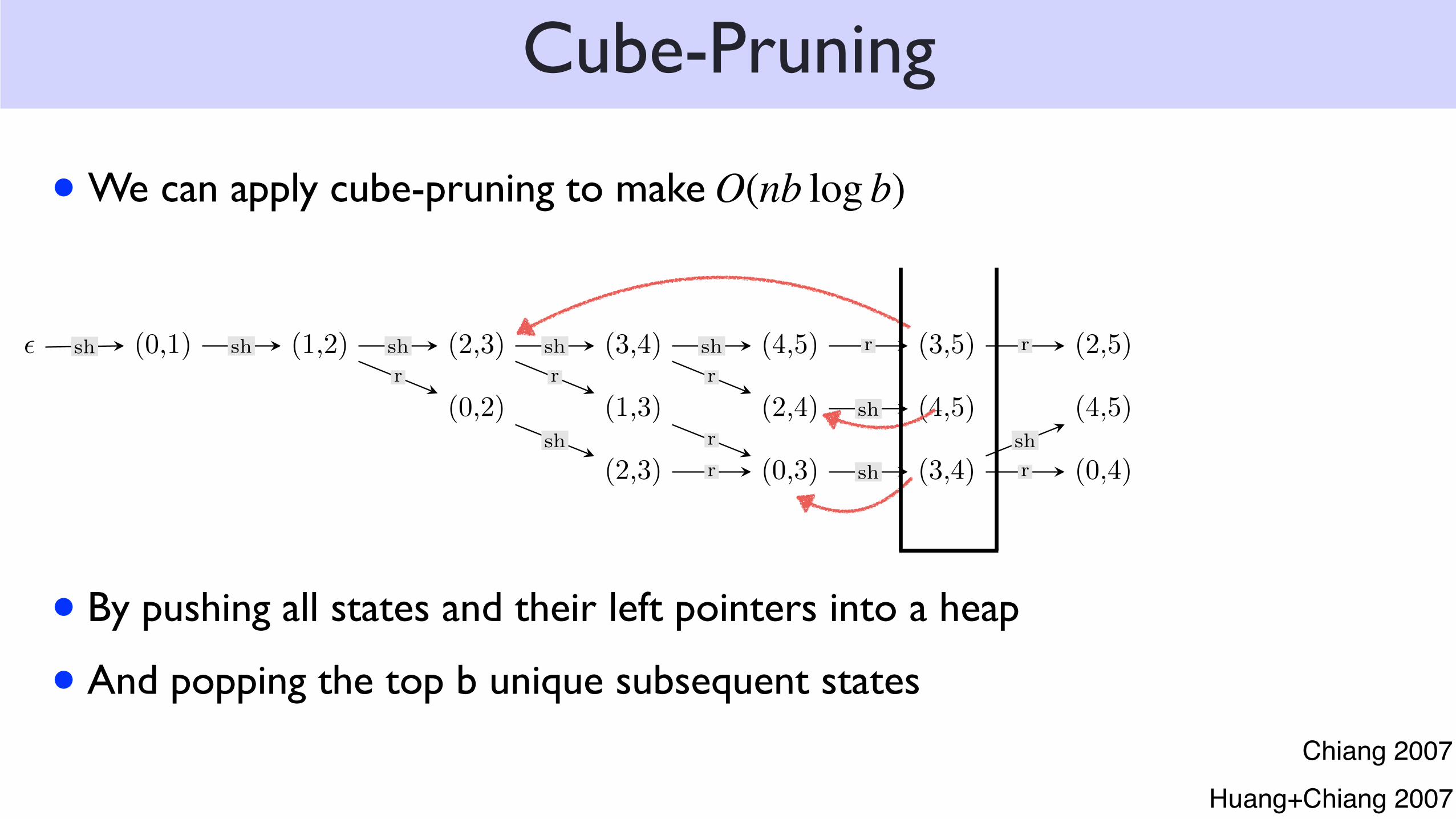
Cube-Pruning
37
• By pushing all states and their left pointers into a heap
• And popping the top b unique subsequent states
• We can apply cube-pruning to make O(nb log b)
Chiang 2007
Huang+Chiang 2007
✏ (0,1) (1,2) (2,3) (3,4) (4,5) (3,5) (2,5) (1,5) (0,5)
(0,2) (1,3) (2,4) (4,5) (4,5) (3,5)
(2,3) (0,3) (3,4) (0,4) (4,5)
sh sh sh
r
sh
r
sh
sh
r
r
r
r
sh
sh
r
sh
r
r
r
sh
r
r
r
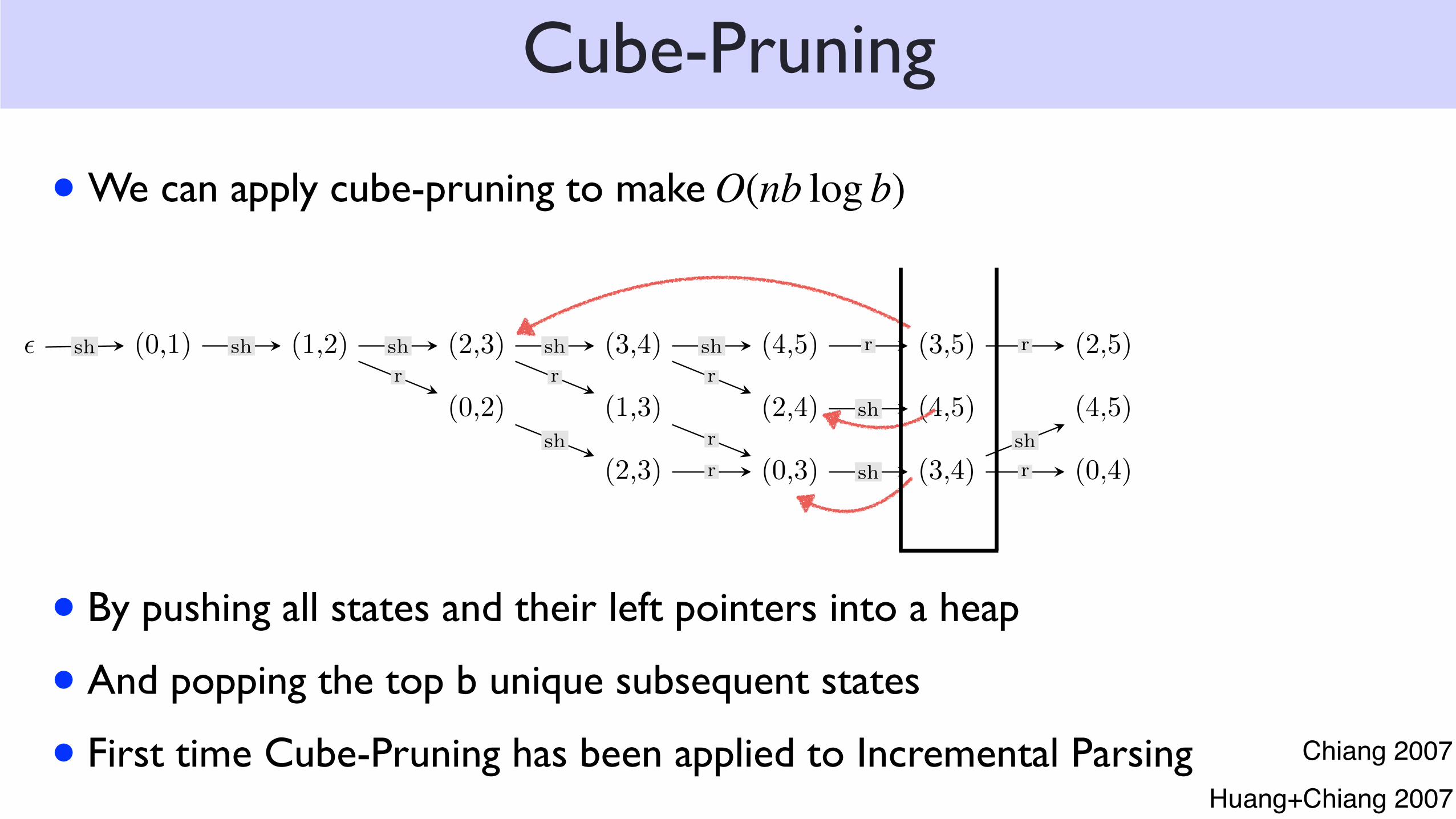
Cube-Pruning
• By pushing all states and their left pointers into a heap
• And popping the top b unique subsequent states
• First time Cube-Pruning has been applied to Incremental Parsing
• We can apply cube-pruning to make O(nb log b)
Chiang 2007
Huang+Chiang 2007
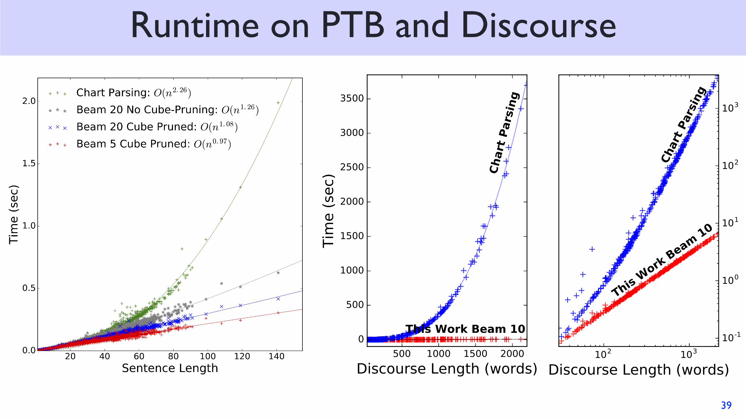
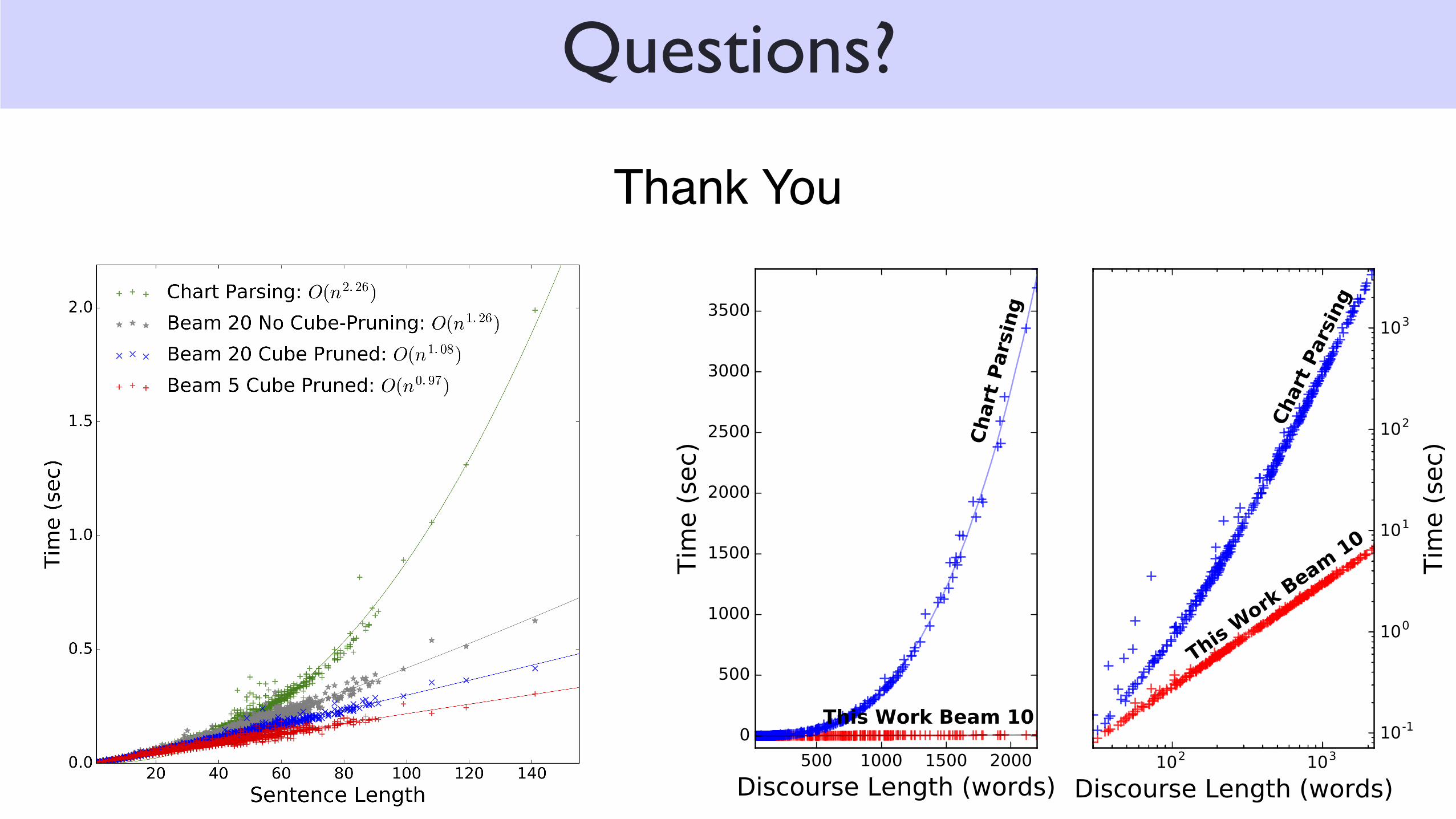
Runtime on PTB and Discourse
39
Training
40
Training
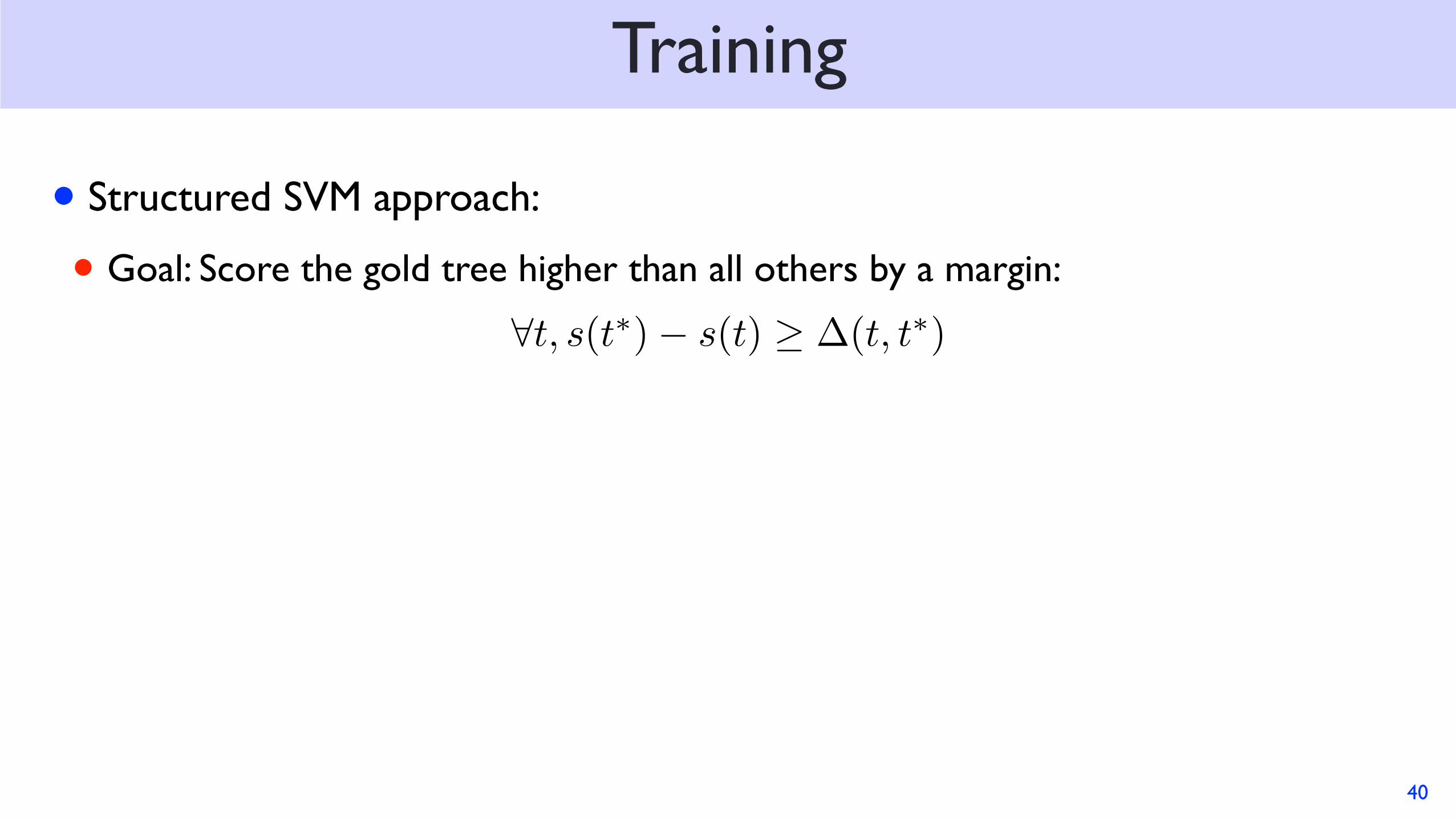
• Structured SVM approach:
• Goal: Score the gold tree higher than all others by a margin:
40
8t, s(t⇤)� s(t) � �(t, t⇤)
Training
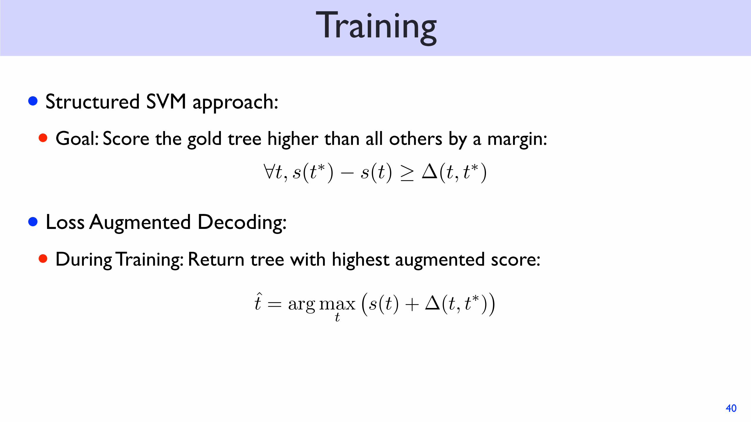
• Structured SVM approach:
• Goal: Score the gold tree higher than all others by a margin:
• Loss Augmented Decoding:
• During Training: Return tree with highest augmented score:
40
8t, s(t⇤)� s(t) � �(t, t⇤)
t̂ = argmaxt
�s(t) +�(t, t⇤)
�
Training
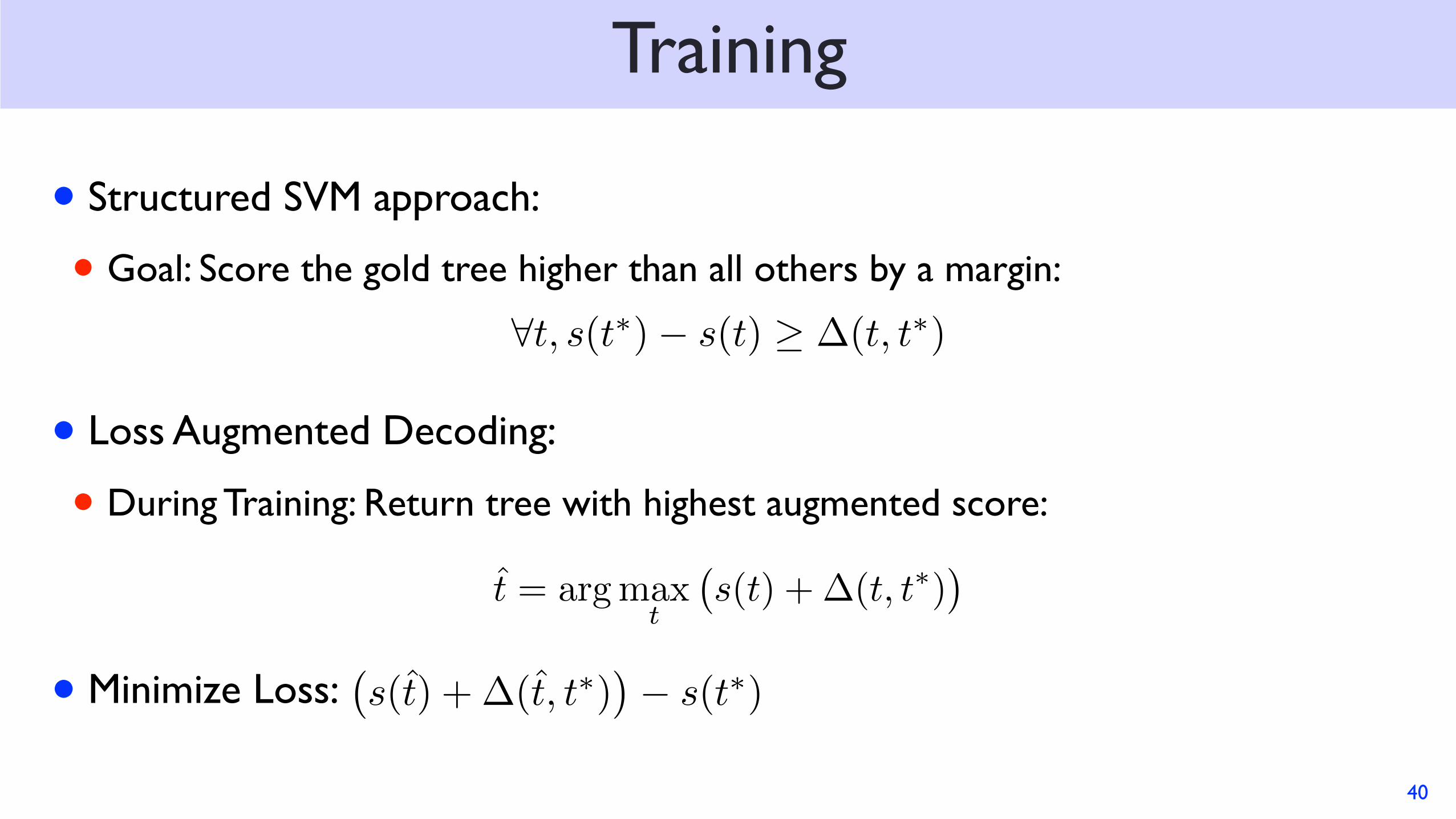
• Structured SVM approach:
• Goal: Score the gold tree higher than all others by a margin:
• Loss Augmented Decoding:
• During Training: Return tree with highest augmented score:
• Minimize Loss:
40
8t, s(t⇤)� s(t) � �(t, t⇤)
t̂ = argmaxt
�s(t) +�(t, t⇤)
�
�s(t̂) +�(t̂, t⇤)
�� s(t⇤)
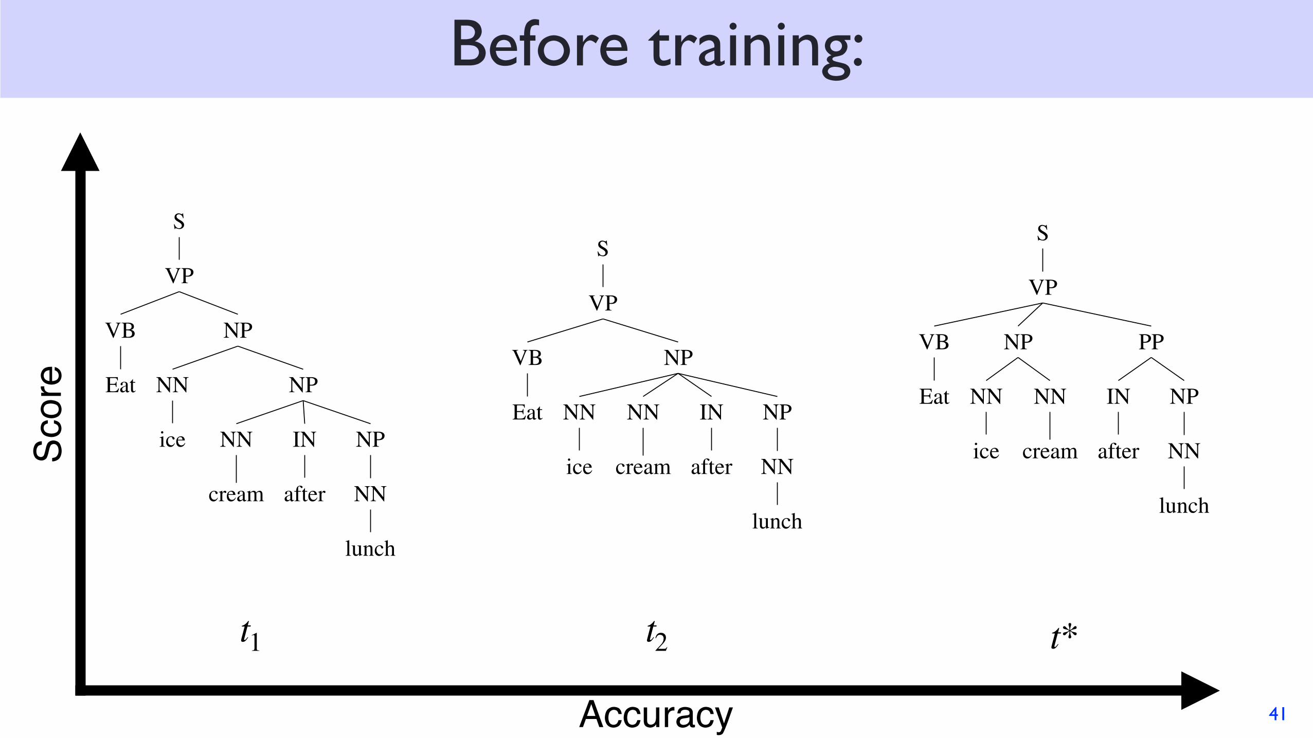
Before training:
41
Scor
e
t*t1 t2
Accuracy
S
VP
NP
NP
NN
lunch
IN
after
NN
cream
NN
ice
VB
Eat
S
VP
NP
NP
NP
NN
lunch
IN
after
NN
cream
NN
ice
VB
Eat
S
VP
PP
NP
NN
lunch
IN
after
NP
NN
cream
NN
ice
VB
Eat
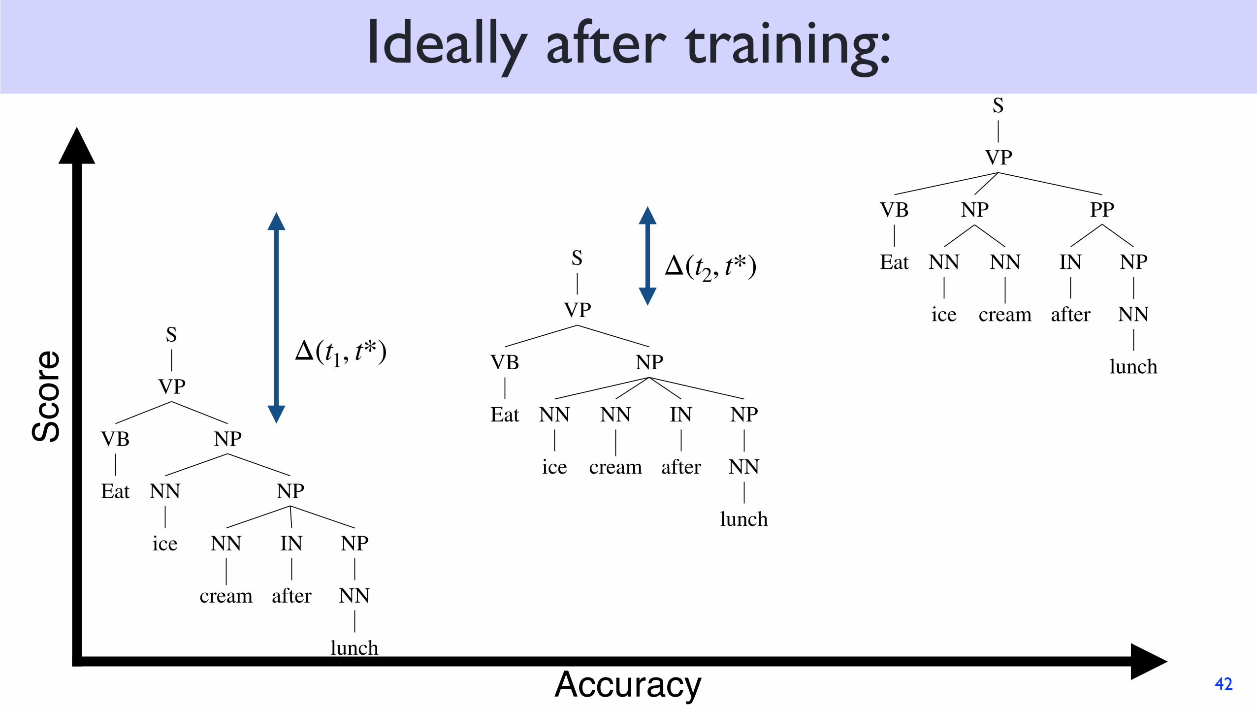
Ideally after training:
42
Scor
e
Accuracy
S
VP
NP
NP
NN
lunch
IN
after
NN
cream
NN
ice
VB
Eat
S
VP
NP
NP
NP
NN
lunch
IN
after
NN
cream
NN
ice
VB
Eat
S
VP
PP
NP
NN
lunch
IN
after
NP
NN
cream
NN
ice
VB
EatΔ(t2, t*)
Δ(t1, t*)

Ideally after training:
43
Scor
e
Accuracy
S
VP
NP
NP
NN
lunch
IN
after
NN
cream
NN
ice
VB
Eat
S
VP
NP
NP
NP
NN
lunch
IN
after
NN
cream
NN
ice
VB
Eat
S
VP
PP
NP
NN
lunch
IN
after
NP
NN
cream
NN
ice
VB
EatΔ(t2, t*)
Δ(t1, t*)
*Y Axis not drawn to scale
Delta Margins
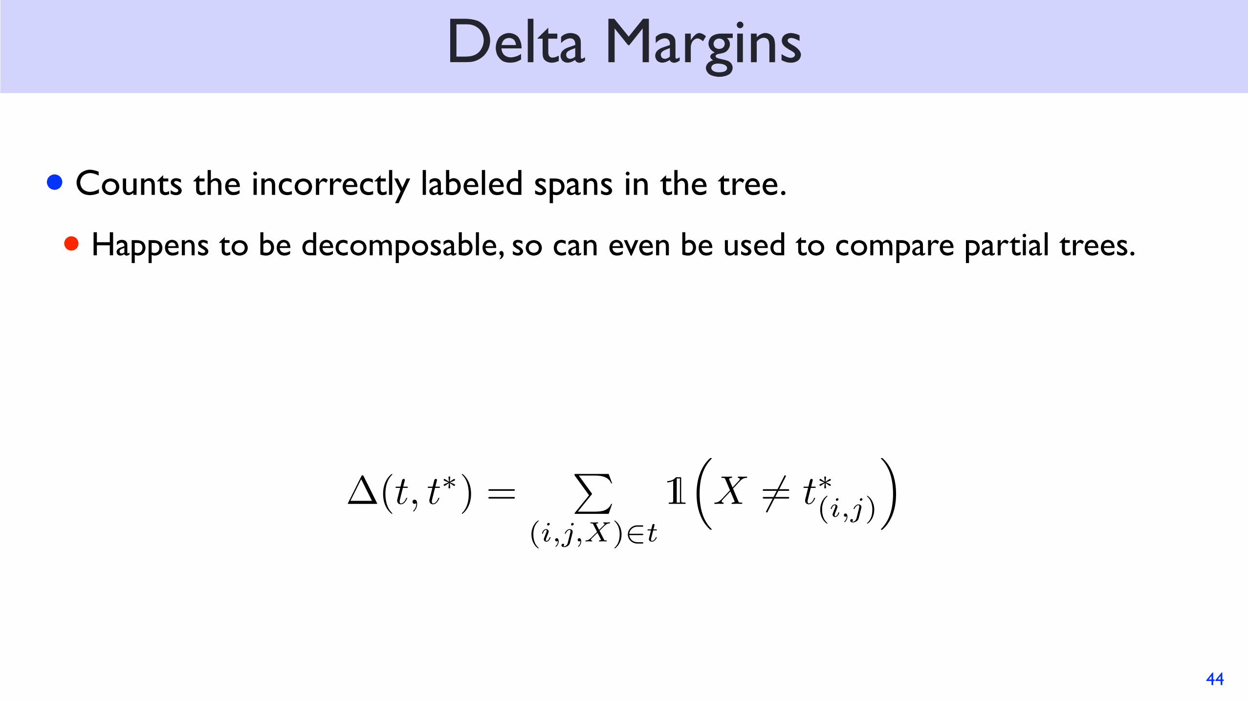
• Counts the incorrectly labeled spans in the tree.
• Happens to be decomposable, so can even be used to compare partial trees.
44
�(t, t⇤) =P
(i,j,X)2t
1⇣X 6= t⇤(i,j)
⌘
Cross-Span Loss
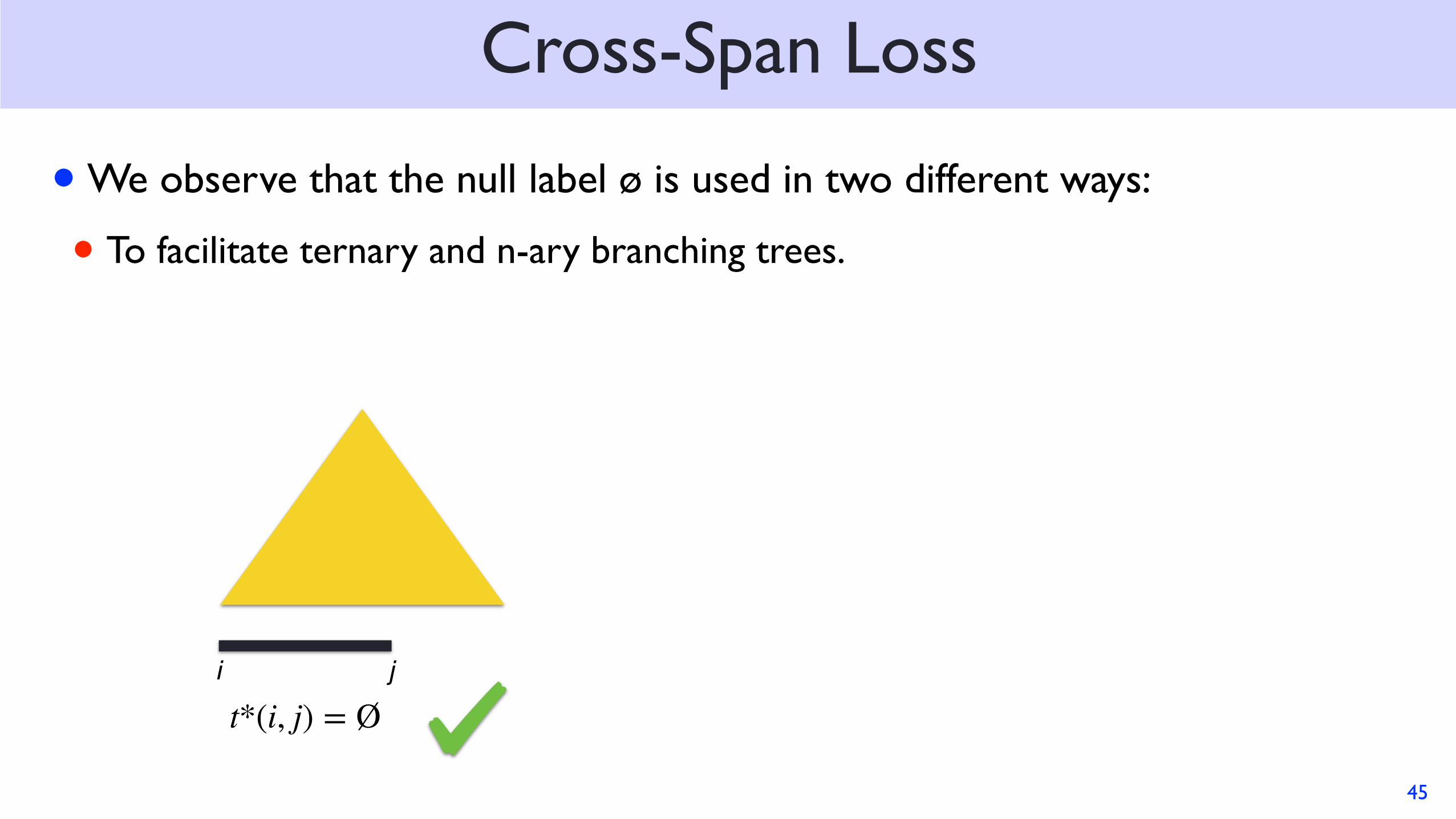
• We observe that the null label ø is used in two different ways:
45
Cross-Span Loss
• We observe that the null label ø is used in two different ways:
• To facilitate ternary and n-ary branching trees.
45
i j
t*(i, j) = Ø
Cross-Span Loss
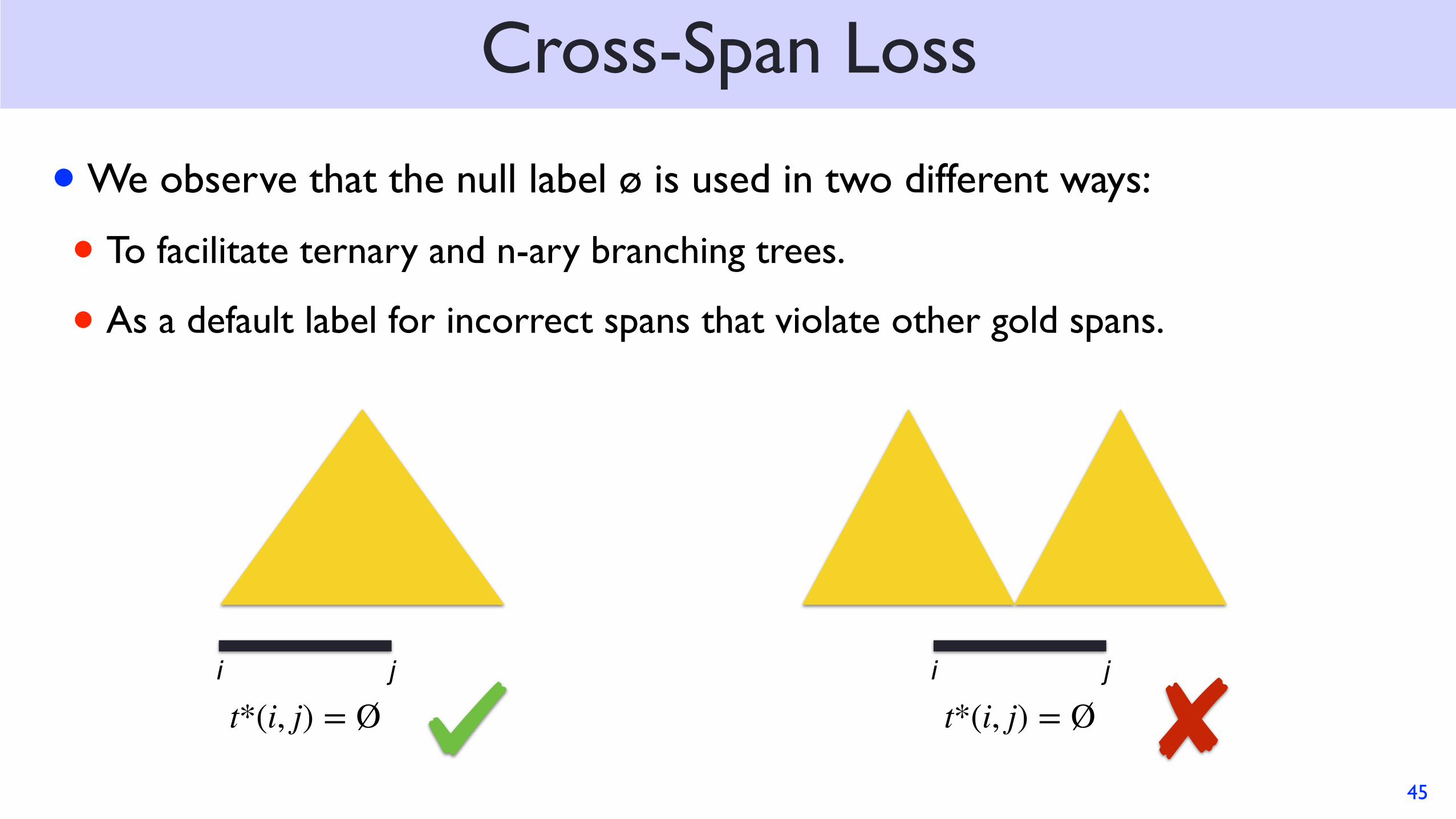
• We observe that the null label ø is used in two different ways:
• To facilitate ternary and n-ary branching trees.
• As a default label for incorrect spans that violate other gold spans.
45
i j
t*(i, j) = Øi j
t*(i, j) = Ø
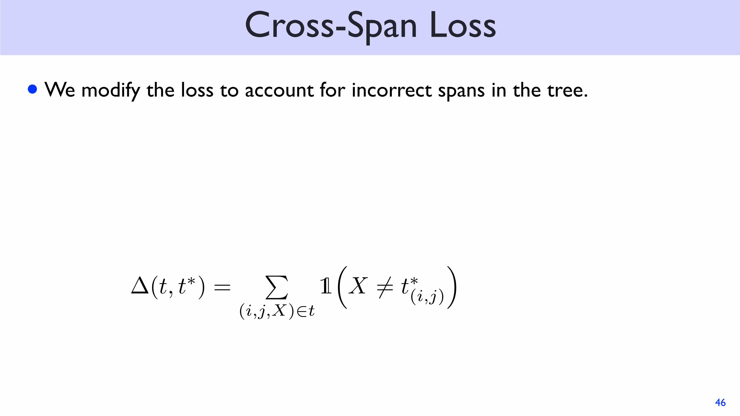
• We modify the loss to account for incorrect spans in the tree.
Cross-Span Loss
46
�(t, t⇤) =P
(i,j,X)2t
1⇣X 6= t⇤(i,j)
⌘

• We modify the loss to account for incorrect spans in the tree.
Cross-Span Loss
47
�(t, t⇤) =P
(i,j,X)2t
1⇣X 6= t⇤(i,j) _ cross(i, j, t⇤)
⌘
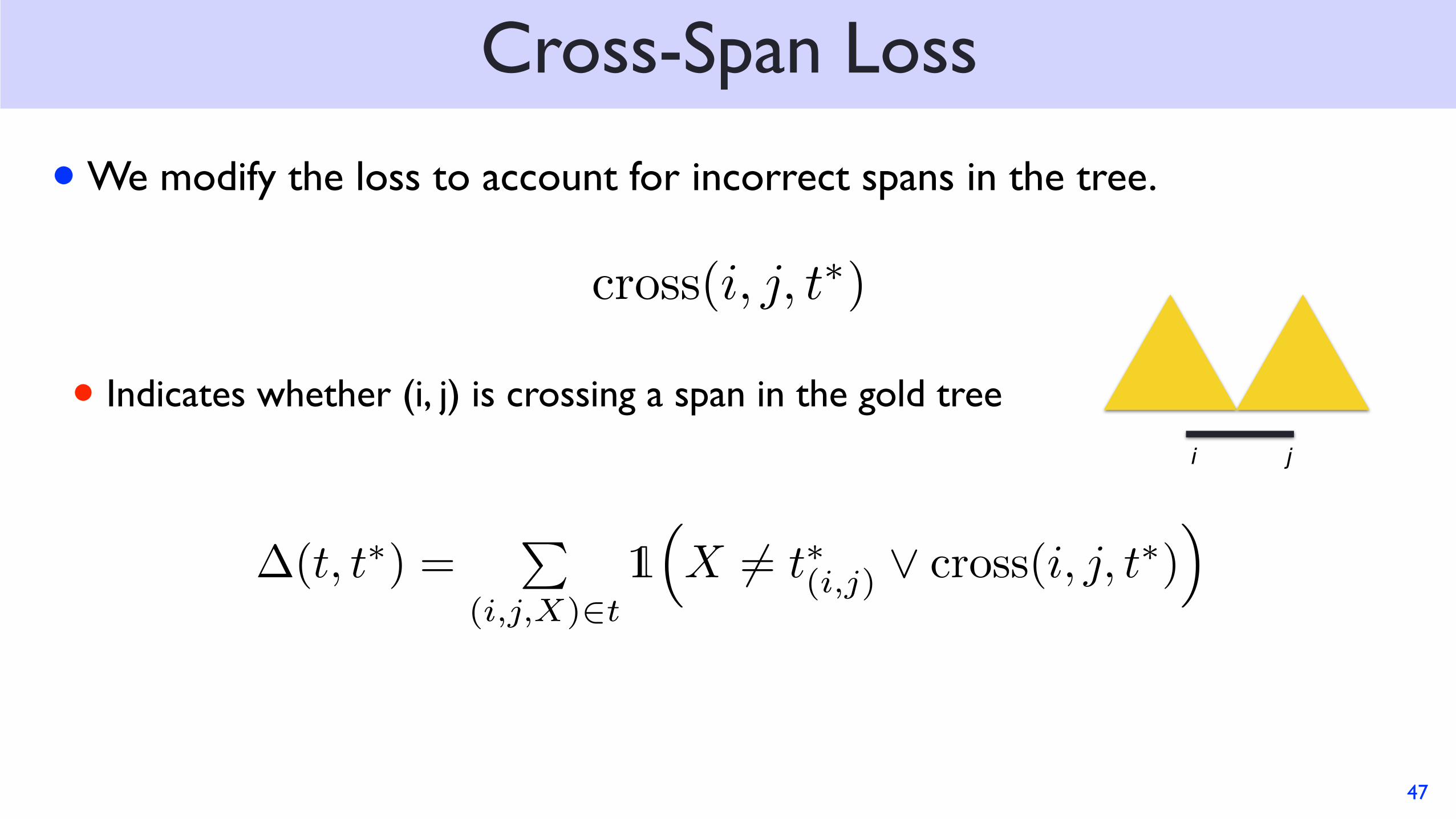
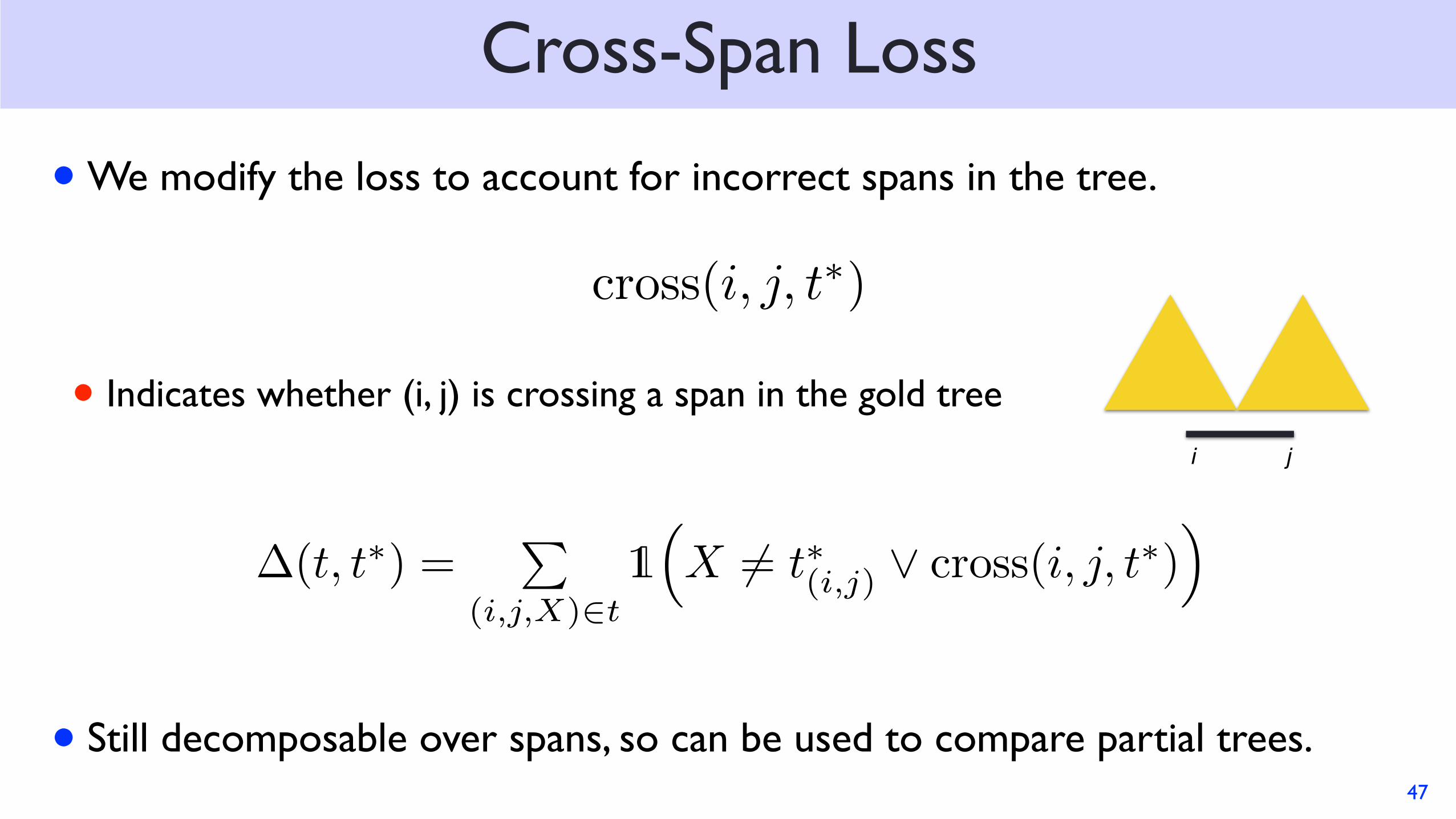
• We modify the loss to account for incorrect spans in the tree.
• Indicates whether (i, j) is crossing a span in the gold tree
cross(i, j, t⇤) = 9 (k, l) 2 t⇤ :
Cross-Span Loss
47
�(t, t⇤) =P
(i,j,X)2t
1⇣X 6= t⇤(i,j) _ cross(i, j, t⇤)
⌘i j
• We modify the loss to account for incorrect spans in the tree.
• Indicates whether (i, j) is crossing a span in the gold tree
• Still decomposable over spans, so can be used to compare partial trees.
cross(i, j, t⇤) = 9 (k, l) 2 t⇤ :
Cross-Span Loss
47
�(t, t⇤) =P
(i,j,X)2t
1⇣X 6= t⇤(i,j) _ cross(i, j, t⇤)
⌘i j
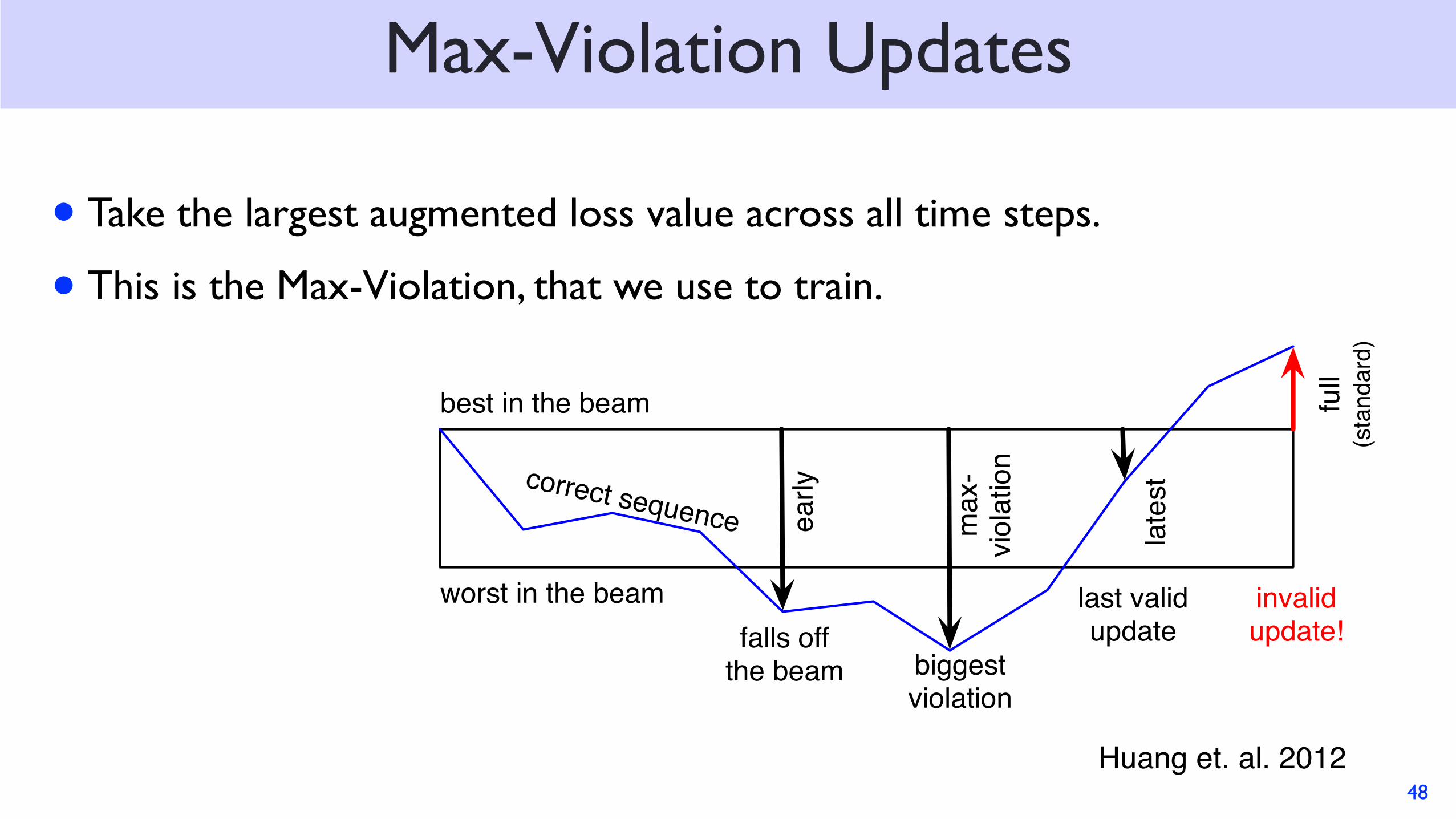
• Take the largest augmented loss value across all time steps.
• This is the Max-Violation, that we use to train.
Max-Violation Updates
48
Huang et. al. 2012ea
rly
max
-vi
olat
ion
late
st
full
(standard)
best in the beam
worst in the beamfalls off
the beam biggestviolation
last valid update
correct sequence
invalidupdate!
Experiments: PTB Test
49
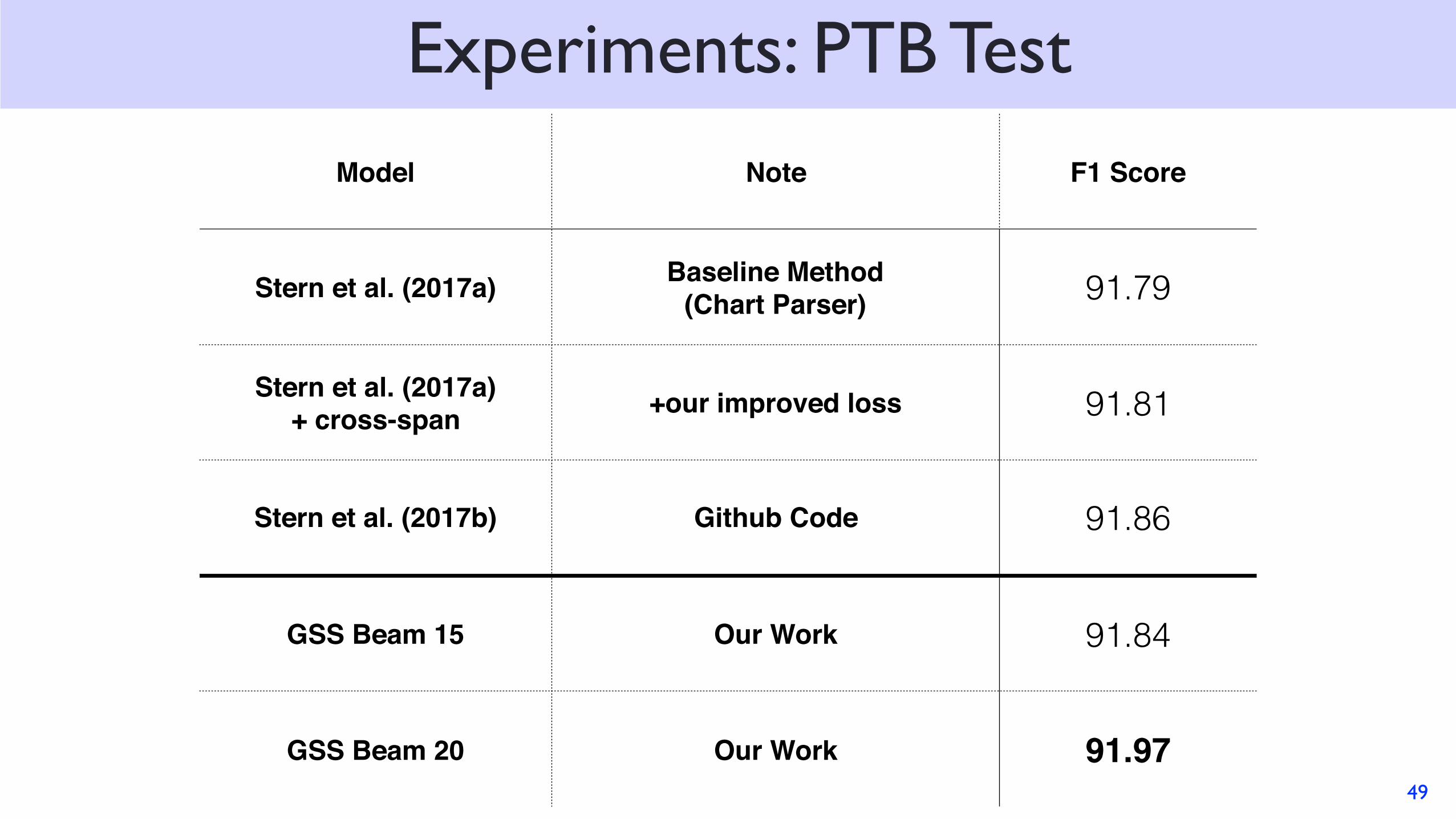
Model Note F1 Score
Stern et al. (2017a) Baseline Method(Chart Parser) 91.79
Stern et al. (2017a) + cross-span +our improved loss 91.81
Stern et al. (2017b) Github Code 91.86
GSS Beam 15 Our Work 91.84
GSS Beam 20 Our Work 91.97
Comparison to other parsers
50
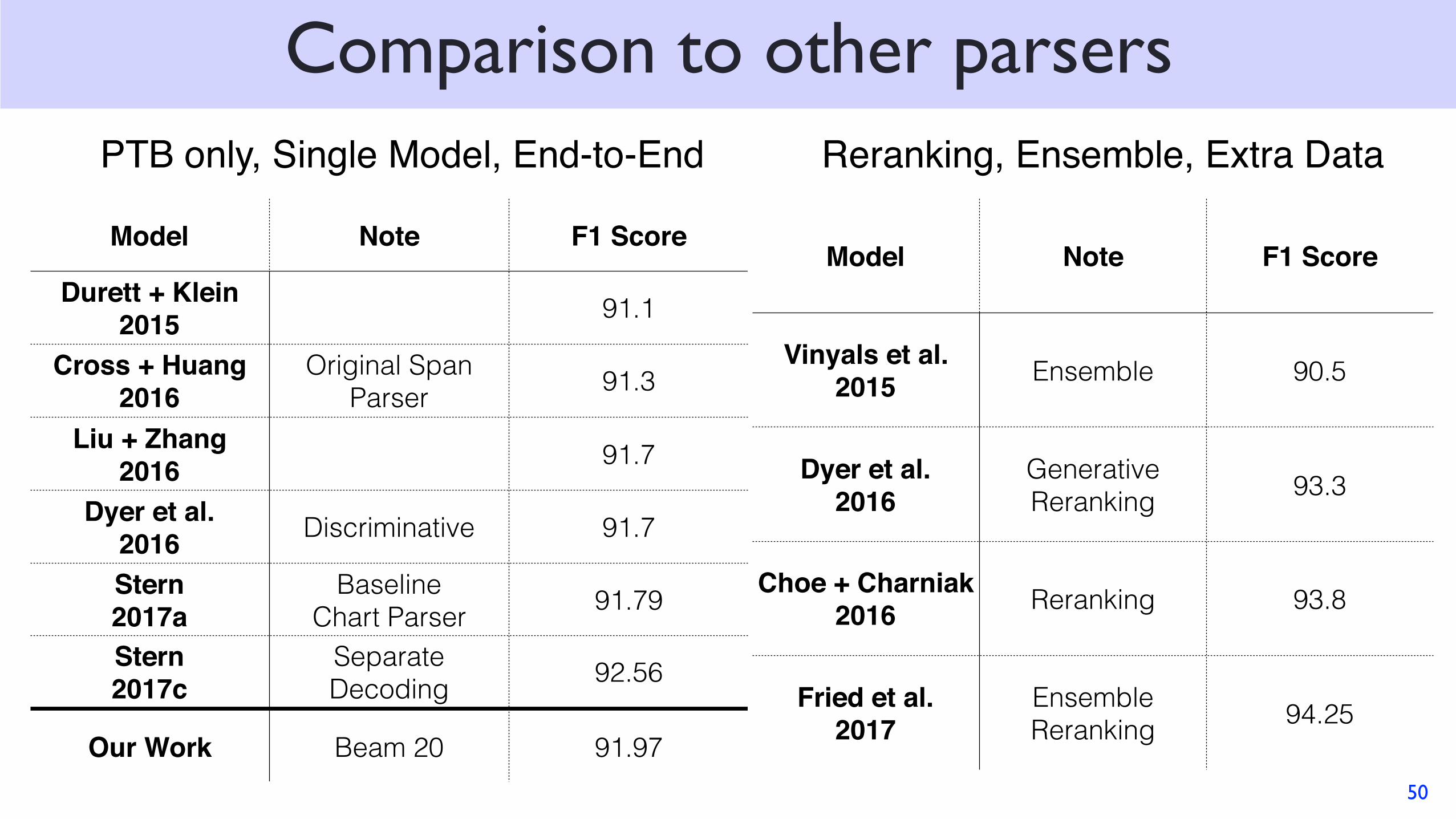
Model Note F1 Score
Durett + Klein2015 91.1
Cross + Huang 2016
Original Span Parser 91.3
Liu + Zhang2016 91.7
Dyer et al. 2016 Discriminative 91.7
Stern 2017a
Baseline Chart Parser 91.79
Stern 2017c
Separate Decoding 92.56
Our Work Beam 20 91.97
Model Note F1 Score
Vinyals et al.2015 Ensemble 90.5
Dyer et al.2016
Generative Reranking 93.3
Choe + Charniak2016 Reranking 93.8
Fried et al.2017
Ensemble Reranking 94.25
Reranking, Ensemble, Extra DataPTB only, Single Model, End-to-End
Conclusions:
• Linear Time Span-Based Constituency Parsing with Dynamic Programming.
• Cube-Pruning to speedup Incremental Parsing with Dynamic Programming.
• Cross-Span Loss extension for improving Loss-Augmented Decoding.
• Result: Faster and more accurate than cubic-time Chart Parsing.
51
Caveats:
• 2nd highest accuracy for single-model end-to-end systems trained on PTB only.
• Stern et al. 2017c is more accurate, but with separate decoding, and is much slower.
• After this ACL, definitely no longer true. (e.g. Joshi et al. 2018, Kitaev+Klein 2018)
• But both are Span-Based Parsers and can be linearized in the same way!
52
Questions?
53
Thank You