Linear Structural Relations (LISREL and R)

Comparing results for various models

eta1

Y1

Y2

Y3

eta2

Y4

Y5

Y6

Xi1

X1

X2

X3

Xi2

X4

X5

X6

Xi3

X7

X8

X9

eps1

eps2

eps3

eps4

eps5

eps6

eps7

eps8

eps9

theta1

theta2

theta3

theta4

theta5

theta6

Error X Observed X Latent X Latent Y Observed Y Error Y

Basic Lisrel model

Multiple programs: multiple syntaxes

I. Commerical packages

A.LISREL (Karl Jöreskog & Dag Sörbom)

B. EQS (Peter Bentler)

C. MPlus (Muthén & Muthén)

II. Open Source/Free

A. sem (John Fox)

B. Mx (Michael Neale)3

sem, R, LISREL

I. R is available for download at CRAN

A.sem package needs to be installed

II. LISREL is available at Social Science Compute Cluster

A.Can be run remotely

4

Using the SSCCvpn166129:~ bill$ ssh revelle@hardin.it.northwestern.edurevelle@hardin.it.northwestern.edu's password: Last login: Mon Feb 12 10:57:28 2007 from vpn166129.vpn.northwestern.edu

Northwestern University Social Sciences Computing Cluster

Academic Technologies / Research Computing

Please report system anomalies to action@hardin.it.northwestern.edu

--- Date -- -------------------- Description -------------------------Feb 06 2007 AMD Core Math Library acml 3.6.0 installedConnection to hardin.it.northwestern.edu closed.vpn166129:~ bill$ ssh revelle@hardin.it.northwestern.edurevelle@hardin.it.northwestern.edu's password: Last login: Tue Feb 13 14:27:21 2007 from vpn166212.vpn.northwestern.edu

Northwestern University Social Sciences Computing Cluster

Academic Technologies / Research Computing

Please report system anomalies to action@hardin.it.northwestern.edu

--- Date -- -------------------- Description -------------------------Feb 06 2007 AMD Core Math Library acml 3.6.0 installedFeb 02 2007 matlab6 (32-bit, version 6.5, R13sp1) returned to serviceFeb 01 2007 Stat/Transfer Upgraded to Version 8.2.7.0120Jan 25 2007 X-Win32 8.1 Available http://www.at.northwestern.edu/x-win32/Nov 16 2006 ox release 4.04 (x64) installedNov 02 2006 gauss release 8.0.0 (x64) installedOct 09 2006 SSCC hardware upgraded

See the complete list of Social Sciences Computing Cluster bulletins athttp://sscc.northwestern.edu/bull/index.cfm

list the directory[revelle@hardin ~]$ ls -ltotal 156-rw------- 1 revelle users 836 Dec 25 19:31 GUTHRIE.DSF-rw------- 1 revelle users 2100 Dec 25 19:31 guthrie.FIT-rw------- 1 revelle users 6736 Dec 25 19:31 guthrie.MSF-rw-r--r-- 1 revelle users 284 Dec 25 19:30 guthrie.txt-rw------- 1 revelle users 8172 Dec 25 19:31 gut.out-rw------- 1 revelle users 202 Dec 22 11:34 loehlin2.5.txt-rw------- 1 revelle users 935 Dec 25 18:45 lout-rw------- 1 revelle users 1656 Dec 25 18:32 lsq.out-rw------- 1 revelle users 980 Dec 25 19:18 LSQUARE.DSF-rw------- 1 revelle users 1299 Dec 25 19:26 lsquare.out-rw-r--r-- 1 revelle users 606 Dec 25 19:28 lsquare.txt-rw------- 1 revelle users 4660 Dec 23 10:02 myfirstlisrel-rw-r--r-- 1 revelle users 434 Dec 25 08:00 prob2.5-rw------- 1 revelle users 5037 Dec 25 07:59 prob2.5.out-rw------- 1 revelle users 708 Dec 25 07:59 PROB2.DSF-rw------- 1 revelle users 5604 Dec 25 07:59 prob2.MSF-rw------- 1 revelle users 1316 Feb 12 11:37 RM5A.DSF-rw------- 1 revelle users 15188 Feb 12 11:37 rm5a.MSF-rw------- 1 revelle users 11561 Feb 12 11:37 rm5a.out-rw-r--r-- 1 revelle users 685 Feb 12 11:36 rm5a.txt-rw------- 1 revelle users 1316 Feb 14 10:57 RM5.DSF-rw------- 1 revelle users 15188 Feb 14 10:57 rm5.MSF-rw------- 1 revelle users 9780 Feb 14 10:57 rm5.out-rw-r--r-- 1 revelle users 601 Feb 12 10:59 rm5.txt

submit a jobI. Upload the control statements using sftp

II. submit the job

A. [revelle@hardin ~]$ lisrel8 rm5.txt rm5.out

III.move the output back to your desktop using sftp

IV. Repeat until satisfied

V. logout

7

A specific modelI. Junior Year

A. Induction

B. Figural Ability

II. Senior Year

A.Figural Ability

III. Prediction model

A. Induction -> Figural Ability in both years

B. Figural ability (jr) -> Figural ability (sr)

IV.Taken from Rakov and Marcoulides (2006)8

Measures are imperfect

I. Multiple measures of each construct

II. Construct is what ever is common to the multiple measures

9

A specific model

Induction Figural Fig2

Induction1 Induction2 Induction3 Figural1 Figural2 Figural3 Fig2_1 Fig2_2 Fig2_3

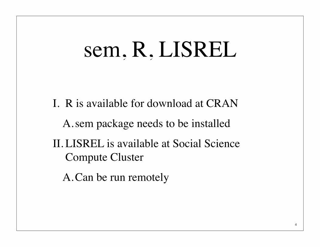
Covariance/Correlations

56.21 31.55 75.55 23.27 28.30 44.45 24.48 32.24 22.56 84.64 22.51 29.54 20.61 57.61 78.93 22.65 27.56 15.33 53.57 49.27 73.76 33.24 46.49 31.44 67.81 54.76 54.58 141.77 32.56 40.37 25.58 55.82 52.33 47.74 98.62 117.33 30.32 40.44 27.69 54.78 53.44 59.52 96.95 84.87 106.35

Rectangular or Triangular

Induct1 Induct2 Induct3 Figural1 Figural2 Figural3 Fig2.1 Fig2.2 Fig2.3Induct1 56.21 31.55 23.27 24.48 22.51 22.65 33.24 32.56 30.32Induct2 31.55 75.55 28.30 32.24 29.54 27.56 46.49 40.37 40.44Induct3 23.27 28.30 44.45 22.56 20.61 15.33 31.44 25.58 27.69Figural1 24.48 32.24 22.56 84.64 57.61 53.57 67.81 55.82 54.78Figural2 22.51 29.54 20.61 57.61 78.93 49.27 54.76 52.33 53.44Figural3 22.65 27.56 15.33 53.57 49.27 73.76 54.58 47.74 59.52Fig2.1 33.24 46.49 31.44 67.81 54.76 54.58 141.77 98.62 96.95Fig2.2 32.56 40.37 25.58 55.82 52.33 47.74 98.62 117.33 84.87Fig2.3 30.32 40.44 27.69 54.78 53.44 59.52 96.95 84.87 106.35

prob5

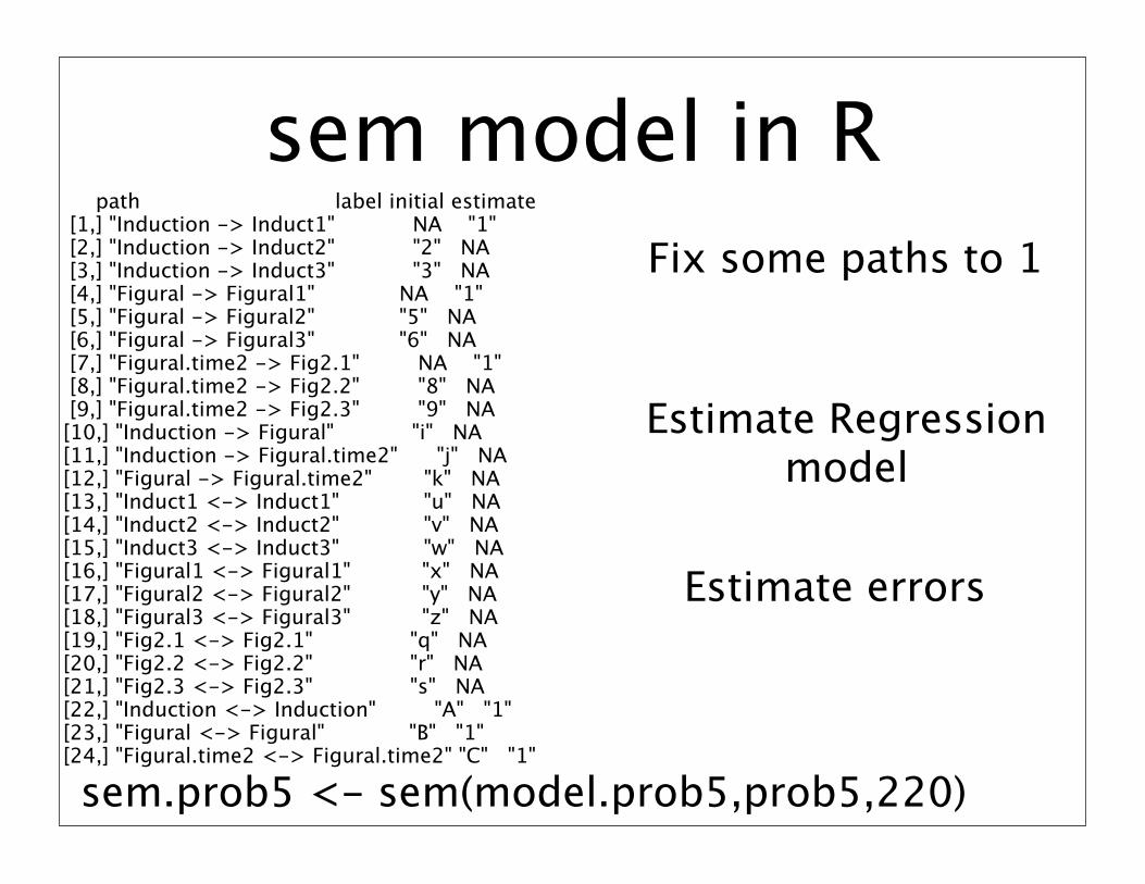
sem model in R path label initial estimate [1,] "Induction -> Induct1" NA "1" [2,] "Induction -> Induct2" "2" NA [3,] "Induction -> Induct3" "3" NA [4,] "Figural -> Figural1" NA "1" [5,] "Figural -> Figural2" "5" NA [6,] "Figural -> Figural3" "6" NA [7,] "Figural.time2 -> Fig2.1" NA "1" [8,] "Figural.time2 -> Fig2.2" "8" NA [9,] "Figural.time2 -> Fig2.3" "9" NA [10,] "Induction -> Figural" "i" NA [11,] "Induction -> Figural.time2" "j" NA [12,] "Figural -> Figural.time2" "k" NA [13,] "Induct1 <-> Induct1" "u" NA [14,] "Induct2 <-> Induct2" "v" NA [15,] "Induct3 <-> Induct3" "w" NA [16,] "Figural1 <-> Figural1" "x" NA [17,] "Figural2 <-> Figural2" "y" NA [18,] "Figural3 <-> Figural3" "z" NA [19,] "Fig2.1 <-> Fig2.1" "q" NA [20,] "Fig2.2 <-> Fig2.2" "r" NA [21,] "Fig2.3 <-> Fig2.3" "s" NA [22,] "Induction <-> Induction" "A" "1" [23,] "Figural <-> Figural" "B" "1" [24,] "Figural.time2 <-> Figural.time2" "C" "1"

Fix some paths to 1

Estimate errors

Estimate Regression model

sem.prob5 <- sem(model.prob5,prob5,220)

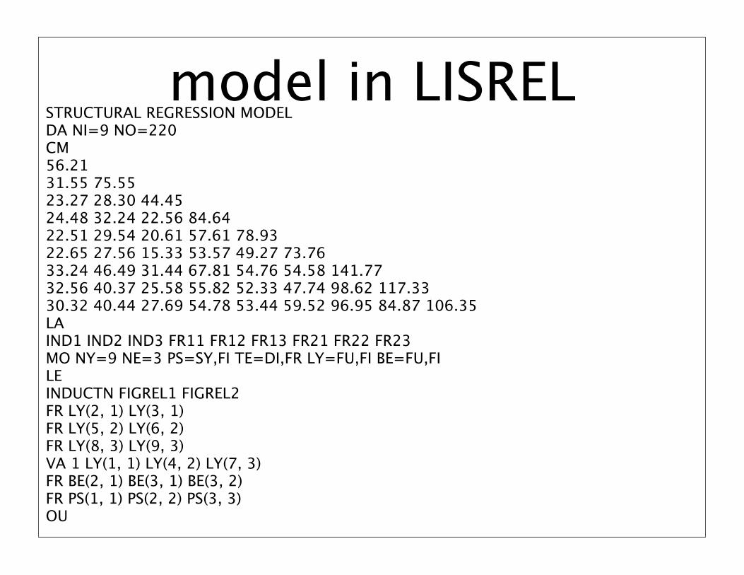
model in LISREL STRUCTURAL REGRESSION MODEL DA NI=9 NO=220 CM 56.21 31.55 75.55 23.27 28.30 44.45 24.48 32.24 22.56 84.64 22.51 29.54 20.61 57.61 78.93 22.65 27.56 15.33 53.57 49.27 73.76 33.24 46.49 31.44 67.81 54.76 54.58 141.77 32.56 40.37 25.58 55.82 52.33 47.74 98.62 117.33 30.32 40.44 27.69 54.78 53.44 59.52 96.95 84.87 106.35 LA IND1 IND2 IND3 FR11 FR12 FR13 FR21 FR22 FR23 MO NY=9 NE=3 PS=SY,FI TE=DI,FR LY=FU,FI BE=FU,FI LE INDUCTN FIGREL1 FIGREL2 FR LY(2, 1) LY(3, 1) FR LY(5, 2) LY(6, 2) FR LY(8, 3) LY(9, 3) VA 1 LY(1, 1) LY(4, 2) LY(7, 3) FR BE(2, 1) BE(3, 1) BE(3, 2) FR PS(1, 1) PS(2, 2) PS(3, 3) OU

oops, sem doesn’t convergeWarning messages:1: Optimization may not have converged; nlm return code = 4. Consult ?nlm. in: sem.default(ram = ram, S = S, N = N, param.names = pars, var.names = vars, 2: Negative parameter variances.Model is probably underidentified. in: sem.default(ram = ram, S = S, N = N, param.names = pars, var.names = vars, > summary(sem.prob5,digits=2)

Model Chisquare = 124 Df = 24 Pr(>Chisq) = 2.1e-15 Chisquare (null model) = 1177 Df = 36 Goodness-of-fit index = 0.88 Adjusted goodness-of-fit index = 0.78 RMSEA index = 0.14 90% CI: (0.11, 0.16) Bentler-Bonnett NFI = 0.9 Tucker-Lewis NNFI = 0.87 Bentler CFI = 0.91 BIC = -5.7

Parameters are weird

Parameter Estimates Estimate Std Error z value Pr(>|z|) 2 1.3e+00 0.118 10.6 0.0e+00 Induct2 <--- Induction 3 8.5e-01 0.100 8.5 0.0e+00 Induct3 <--- Induction 5 9.3e-01 0.026 35.3 0.0e+00 Figural2 <--- Figural 6 8.8e-01 0.021 42.0 0.0e+00 Figural3 <--- Figural 8 8.8e-01 0.039 22.4 0.0e+00 Fig2.2 <--- Figural.time2 9 8.8e-01 0.028 31.8 0.0e+00 Fig2.3 <--- Figural.time2 i 2.0e+00 NaN NaN NaN Figural <--- Induction j -2.0e+03 NaN NaN NaN Figural.time2 <--- Induction k 1.0e+03 NaN NaN NaN Figural.time2 <--- Figural u 4.2e+01 4.210 10.0 0.0e+00 Induct1 <--> Induct1 v 5.3e+01 5.350 9.9 0.0e+00 Induct2 <--> Induct2 w 3.4e+01 3.391 10.0 0.0e+00 Induct3 <--> Induct3 x 2.6e+01 3.040 8.5 0.0e+00 Figural1 <--> Figural1 y 2.9e+01 3.535 8.2 2.2e-16 Figural2 <--> Figural2 z 2.8e+01 3.382 8.3 0.0e+00 Figural3 <--> Figural3 q 3.2e+01 4.232 7.5 8.5e-14 Fig2.1 <--> Fig2.1 r 3.2e+01 4.058 8.0 1.8e-15 Fig2.2 <--> Fig2.2 s 2.0e+01 3.050 6.6 3.6e-11 Fig2.3 <--> Fig2.3 A 1.4e+01 NaN NaN NaN Induction <--> Induction B -7.0e-04 NaN NaN NaN Figural <--> Figural C 7.4e+02 NaN NaN NaN Figural.time2 <--> Figural.time2

Iterations = 500

Aliased parameters: i j k A B C Warning message:NaNs produced in: sqrt(diag(object$cov))

Respecify start values

path label initial estimate [1,] "Induction -> Induct1" NA "1" [2,] "Induction -> Induct2" "2" NA [3,] "Induction -> Induct3" "3" NA [4,] "Figural -> Figural1" NA "1" [5,] "Figural -> Figural2" "5" NA [6,] "Figural -> Figural3" "6" NA [7,] "Figural.time2 -> Fig2.1" NA "1" [8,] "Figural.time2 -> Fig2.2" "8" NA [9,] "Figural.time2 -> Fig2.3" "9" NA [10,] "Induction -> Figural" "i" NA [11,] "Induction -> Figural.time2" "j" NA [12,] "Figural -> Figural.time2" "k" "0.75" [13,] "Induct1 <-> Induct1" "u" NA [14,] "Induct2 <-> Induct2" "v" NA [15,] "Induct3 <-> Induct3" "w" NA [16,] "Figural1 <-> Figural1" "x" NA [17,] "Figural2 <-> Figural2" "y" NA [18,] "Figural3 <-> Figural3" "z" NA [19,] "Fig2.1 <-> Fig2.1" "q" NA [20,] "Fig2.2 <-> Fig2.2" "r" NA [21,] "Fig2.3 <-> Fig2.3" "s" NA [22,] "Induction <-> Induction" "A" "1" [23,] "Figural <-> Figural" "B" "1" [24,] "Figural.time2 <-> Figural.time2" "C" "1"

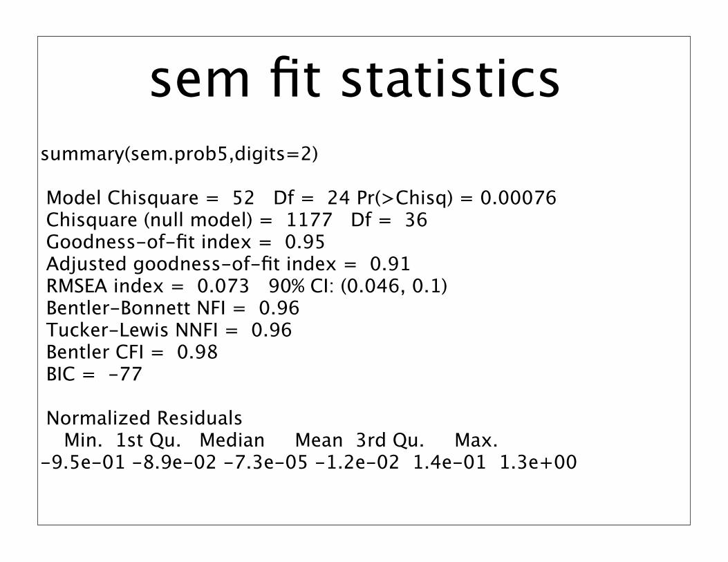
sem fit statisticssummary(sem.prob5,digits=2)

Model Chisquare = 52 Df = 24 Pr(>Chisq) = 0.00076 Chisquare (null model) = 1177 Df = 36 Goodness-of-fit index = 0.95 Adjusted goodness-of-fit index = 0.91 RMSEA index = 0.073 90% CI: (0.046, 0.1) Bentler-Bonnett NFI = 0.96 Tucker-Lewis NNFI = 0.96 Bentler CFI = 0.98 BIC = -77

Normalized Residuals Min. 1st Qu. Median Mean 3rd Qu. Max. -9.5e-01 -8.9e-02 -7.3e-05 -1.2e-02 1.4e-01 1.3e+00

LISREL fits

Goodness of Fit Statistics

Degrees of Freedom = 24 Minimum Fit Function Chi-Square = 52.10 (P = 0.00076) Normal Theory Weighted Least Squares Chi-Square = 48.28 (P = 0.0023) Estimated Non-centrality Parameter (NCP) = 24.28 90 Percent Confidence Interval for NCP = (8.23 ; 48.09) Minimum Fit Function Value = 0.24 Population Discrepancy Function Value (F0) = 0.11 90 Percent Confidence Interval for F0 = (0.038 ; 0.22) Root Mean Square Error of Approximation (RMSEA) = 0.068 90 Percent Confidence Interval for RMSEA = (0.040 ; 0.096) P-Value for Test of Close Fit (RMSEA < 0.05) = 0.14 Expected Cross-Validation Index (ECVI) = 0.41 90 Percent Confidence Interval for ECVI = (0.34 ; 0.52) ECVI for Saturated Model = 0.41 ECVI for Independence Model = 9.49 Chi-Square for Independence Model with 36 Degrees of Freedom = 2060.02 Independence AIC = 2078.02 Model AIC = 90.28 Saturated AIC = 90.00 Independence CAIC = 2117.56 Model CAIC = 182.54 Saturated CAIC = 287.71 Normed Fit Index (NFI) = 0.97 Non-Normed Fit Index (NNFI) = 0.98 Parsimony Normed Fit Index (PNFI) = 0.65 Comparative Fit Index (CFI) = 0.99 Incremental Fit Index (IFI) = 0.99 Relative Fit Index (RFI) = 0.96 Critical N (CN) = 181.68 Root Mean Square Residual (RMR) = 1.99 Standardized RMR = 0.023 Goodness of Fit Index (GFI) = 0.95 Adjusted Goodness of Fit Index (AGFI) = 0.91 Parsimony Goodness of Fit Index (PGFI) = 0.51

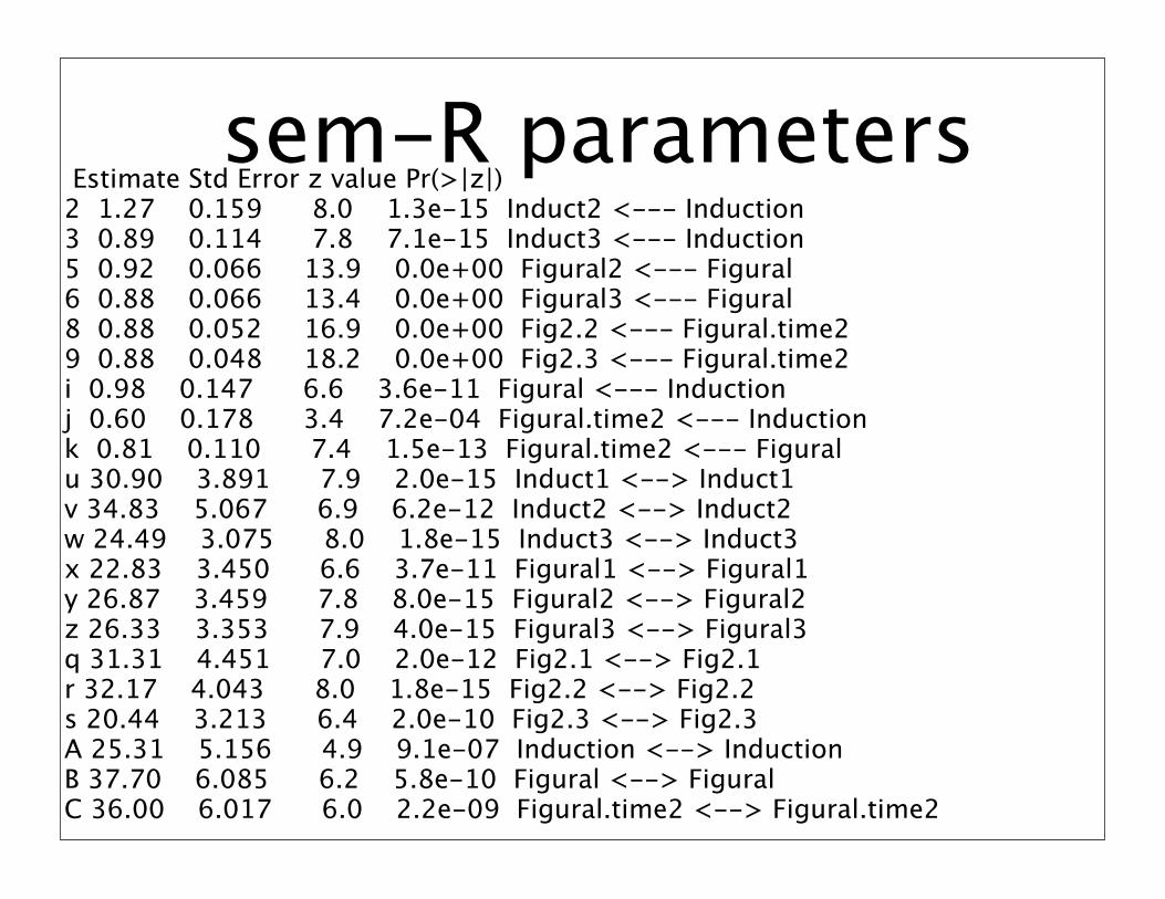
sem-R parameters Estimate Std Error z value Pr(>|z|) 2 1.27 0.159 8.0 1.3e-15 Induct2 <--- Induction 3 0.89 0.114 7.8 7.1e-15 Induct3 <--- Induction 5 0.92 0.066 13.9 0.0e+00 Figural2 <--- Figural 6 0.88 0.066 13.4 0.0e+00 Figural3 <--- Figural 8 0.88 0.052 16.9 0.0e+00 Fig2.2 <--- Figural.time2 9 0.88 0.048 18.2 0.0e+00 Fig2.3 <--- Figural.time2 i 0.98 0.147 6.6 3.6e-11 Figural <--- Induction j 0.60 0.178 3.4 7.2e-04 Figural.time2 <--- Induction k 0.81 0.110 7.4 1.5e-13 Figural.time2 <--- Figural u 30.90 3.891 7.9 2.0e-15 Induct1 <--> Induct1 v 34.83 5.067 6.9 6.2e-12 Induct2 <--> Induct2 w 24.49 3.075 8.0 1.8e-15 Induct3 <--> Induct3 x 22.83 3.450 6.6 3.7e-11 Figural1 <--> Figural1 y 26.87 3.459 7.8 8.0e-15 Figural2 <--> Figural2 z 26.33 3.353 7.9 4.0e-15 Figural3 <--> Figural3 q 31.31 4.451 7.0 2.0e-12 Fig2.1 <--> Fig2.1 r 32.17 4.043 8.0 1.8e-15 Fig2.2 <--> Fig2.2 s 20.44 3.213 6.4 2.0e-10 Fig2.3 <--> Fig2.3 A 25.31 5.156 4.9 9.1e-07 Induction <--> Induction B 37.70 6.085 6.2 5.8e-10 Figural <--> Figural C 36.00 6.017 6.0 2.2e-09 Figural.time2 <--> Figural.time2

LISREL parameters

LAMBDA-Y

INDUCTN FIGREL1 FIGREL2 -------- -------- --------

IND1 1.00 - - - -

IND2 1.27 - - - - (0.16) 8.08

IND3 0.89 - - - -

(0.12) 7.70

FR11 - - 1.00 - -

FR12 - - 0.92 - -

(0.07) 13.76

FR13 - - 0.88 - -

(0.06) 13.54

FR21 - - - - 1.00

FR22 - - - - 0.88

(0.05) 16.79

FR23 - - - - 0.88

(0.05) 18.39

BETA

INDUCTN FIGREL1 FIGREL2 -------- -------- --------

INDUCTN - - - - - -

FIGREL1 0.98 - - - - (0.15) 6.64

FIGREL2 0.60 0.81 - -

(0.18) (0.11) 3.41 7.40

Covariance Matrix of ETA

INDUCTN FIGREL1 FIGREL2 -------- -------- --------

INDUCTN 25.31 FIGREL1 24.71 61.81

FIGREL2 35.39 65.23 110.46

PSI Note: This matrix is diagonal.

INDUCTN FIGREL1 FIGREL2 -------- -------- --------

25.31 37.69 36.00 (5.14) (6.10) (5.92) 4.92 6.18 6.08

sem-R standarized

1 0.67105 Induct1 <--- Induction 2 2 0.73412 Induct2 <--- Induction 3 3 0.67018 Induct3 <--- Induction 4 0.85457 Figural1 <--- Figural 5 5 0.81215 Figural2 <--- Figural 6 6 0.80191 Figural3 <--- Figural 7 0.88269 Fig2.1 <--- Figural.time2 8 8 0.85197 Fig2.2 <--- Figural.time2 9 9 0.89877 Fig2.3 <--- Figural.time2 10 i 0.62464 Figural <--- Induction 11 j 0.28886 Figural.time2 <--- Induction12 k 0.60902 Figural.time2 <--- Figural

Residualsround(residuals(sem.prob5),2)

Induct1 Induct2 Induct3 Figural1 Figural2 Figural3 Fig2.1 Fig2.2 Fig2.3Induct1 0.00 -0.55 0.79 -0.23 -0.17 1.01 -2.15 1.49 -0.89Induct2 -0.55 0.00 -0.21 0.90 0.78 0.11 1.61 0.96 0.86Induct3 0.79 -0.21 0.00 0.62 0.47 -3.89 0.01 -2.02 -0.03Figural1 -0.23 0.90 0.62 0.00 0.88 -0.58 2.58 -1.46 -2.75Figural2 -0.17 0.78 0.47 0.88 0.00 -0.42 -5.11 -0.24 0.64Figural3 1.01 0.11 -3.89 -0.58 -0.42 0.00 -2.56 -2.43 9.13Fig2.1 -2.15 1.61 0.01 2.58 -5.11 -2.56 0.00 1.63 -0.46Fig2.2 1.49 0.96 -2.02 -1.46 -0.24 -2.43 1.63 0.00 -0.67Fig2.3 -0.89 0.86 -0.03 -2.75 0.64 9.13 -0.46 -0.67 0.00

Suggests correlated errors from Figural 3 across time

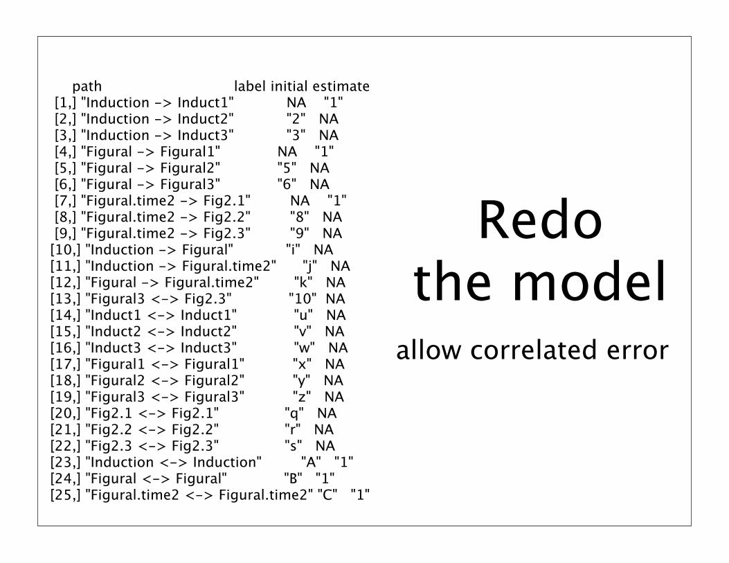
Redo the model

path label initial estimate [1,] "Induction -> Induct1" NA "1" [2,] "Induction -> Induct2" "2" NA [3,] "Induction -> Induct3" "3" NA [4,] "Figural -> Figural1" NA "1" [5,] "Figural -> Figural2" "5" NA [6,] "Figural -> Figural3" "6" NA [7,] "Figural.time2 -> Fig2.1" NA "1" [8,] "Figural.time2 -> Fig2.2" "8" NA [9,] "Figural.time2 -> Fig2.3" "9" NA [10,] "Induction -> Figural" "i" NA [11,] "Induction -> Figural.time2" "j" NA [12,] "Figural -> Figural.time2" "k" NA [13,] "Figural3 <-> Fig2.3" "10" NA [14,] "Induct1 <-> Induct1" "u" NA [15,] "Induct2 <-> Induct2" "v" NA [16,] "Induct3 <-> Induct3" "w" NA [17,] "Figural1 <-> Figural1" "x" NA [18,] "Figural2 <-> Figural2" "y" NA [19,] "Figural3 <-> Figural3" "z" NA [20,] "Fig2.1 <-> Fig2.1" "q" NA [21,] "Fig2.2 <-> Fig2.2" "r" NA [22,] "Fig2.3 <-> Fig2.3" "s" NA [23,] "Induction <-> Induction" "A" "1" [24,] "Figural <-> Figural" "B" "1" [25,] "Figural.time2 <-> Figural.time2" "C" "1"

allow correlated error

LISREL respecified

STRUCTURAL REGRESSION MODELDA NI=9 NO=220CM56.2131.55 75.5523.27 28.30 44.4524.48 32.24 22.56 84.6422.51 29.54 20.61 57.61 78.9322.65 27.56 15.33 53.57 49.27 73.7633.24 46.49 31.44 67.81 54.76 54.58 141.7732.56 40.37 25.58 55.82 52.33 47.74 98.62 117.3330.32 40.44 27.69 54.78 53.44 59.52 96.95 84.87 106.35LAIND1 IND2 IND3 FR11 FR12 FR13 FR21 FR22 FR23MO NY=9 NE=3 PS=SY,FI TE=SY,FI LY=FU,FI BE=FU,FILEINDUCTN FIGREL1 FIGREL2FR LY(2, 1) LY(3, 1)FR LY(5, 2) LY(6, 2)FR LY(8, 3) LY(9, 3)VA 1 LY(1, 1) LY(4, 2) LY(7, 3)FR BE(2, 1) BE(3, 1) BE(3, 2)FR PS(1, 1) PS(2, 2) PS(3, 3)FR TE(1,1) TE (2,2) TE(3,3) TE(4,4) TE(5,5) TE(6,6) TE(7,7) TE(8,8) TE(9,9) TE(9,6)OU

correlated error

Much better fit Model Chisquare = 21 Df = 23 Pr(>Chisq) = 0.61 Chisquare (null model) = 1177 Df = 36 Goodness-of-fit index = 0.98 Adjusted goodness-of-fit index = 0.96 RMSEA index = 0 90% CI: (NA, 0.049) Bentler-Bonnett NFI = 0.98 Tucker-Lewis NNFI = 1 Bentler CFI = 1 BIC = -104

Normalized Residuals Min. 1st Qu. Median Mean 3rd Qu. Max. -8.3e-01 -8.4e-02 1.6e-04 -9.5e-05 1.5e-01 4.5e-01

Chisquare from 52 to 21 with df from 24 to 23but, is this still confirmatory?

sem parametersParameter Estimates Estimate Std Error z value Pr(>|z|) 2 1.27 0.159 8.0 1.3e-15 Induct2 <--- Induction 3 0.89 0.114 7.8 7.1e-15 Induct3 <--- Induction 5 0.92 0.066 13.9 0.0e+00 Figural2 <--- Figural 6 0.88 0.066 13.4 0.0e+00 Figural3 <--- Figural 8 0.88 0.052 16.9 0.0e+00 Fig2.2 <--- Figural.time2 9 0.88 0.048 18.2 0.0e+00 Fig2.3 <--- Figural.time2 i 0.98 0.147 6.6 3.6e-11 Figural <--- Induction j 0.60 0.178 3.4 7.2e-04 Figural.time2 <--- Induction k 0.81 0.110 7.4 1.5e-13 Figural.time2 <--- Figural u 30.90 3.891 7.9 2.0e-15 Induct1 <--> Induct1 v 34.83 5.067 6.9 6.2e-12 Induct2 <--> Induct2 w 24.49 3.075 8.0 1.8e-15 Induct3 <--> Induct3 x 22.83 3.450 6.6 3.7e-11 Figural1 <--> Figural1 y 26.87 3.459 7.8 8.0e-15 Figural2 <--> Figural2 z 26.33 3.353 7.9 4.0e-15 Figural3 <--> Figural3 q 31.31 4.451 7.0 2.0e-12 Fig2.1 <--> Fig2.1 r 32.17 4.043 8.0 1.8e-15 Fig2.2 <--> Fig2.2 s 20.44 3.213 6.4 2.0e-10 Fig2.3 <--> Fig2.3 A 25.31 5.156 4.9 9.1e-07 Induction <--> Induction B 37.70 6.085 6.2 5.8e-10 Figural <--> Figural C 36.00 6.017 6.0 2.2e-09 Figural.time2 <--> Figural.time2

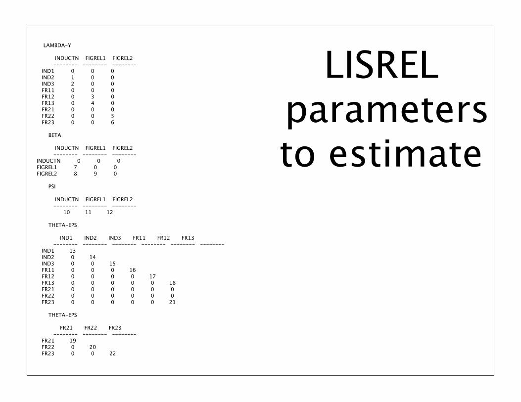
LISREL parametersto estimate

LAMBDA-Y

INDUCTN FIGREL1 FIGREL2 -------- -------- -------- IND1 0 0 0 IND2 1 0 0 IND3 2 0 0 FR11 0 0 0 FR12 0 3 0 FR13 0 4 0 FR21 0 0 0 FR22 0 0 5 FR23 0 0 6

BETA

INDUCTN FIGREL1 FIGREL2 -------- -------- -------- INDUCTN 0 0 0 FIGREL1 7 0 0 FIGREL2 8 9 0

PSI

INDUCTN FIGREL1 FIGREL2 -------- -------- -------- 10 11 12

THETA-EPS

IND1 IND2 IND3 FR11 FR12 FR13 -------- -------- -------- -------- -------- -------- IND1 13 IND2 0 14 IND3 0 0 15 FR11 0 0 0 16 FR12 0 0 0 0 17 FR13 0 0 0 0 0 18 FR21 0 0 0 0 0 0 FR22 0 0 0 0 0 0 FR23 0 0 0 0 0 21

THETA-EPS

FR21 FR22 FR23 -------- -------- -------- FR21 19 FR22 0 20 FR23 0 0 22

LISREL parameters

LAMBDA-Y

INDUCTN FIGREL1 FIGREL2 -------- -------- --------

IND1 1.00 - - - -

IND2 1.27 - - - - (0.16) 8.07

IND3 0.89 - - - -

(0.12) 7.71

FR11 - - 1.00 - -

FR12 - - 0.89 - -

(0.06) 13.89

FR13 - - 0.83 - -

(0.06) 13.46

FR21 - - - - 1.00

FR22 - - - - 0.87

(0.05) 17.20

FR23 - - - - 0.86

(0.05) 18.39

BETA

INDUCTN FIGREL1 FIGREL2 -------- -------- --------

INDUCTN - - - - - -

FIGREL1 1.00 - - - - (0.15) 6.68

FIGREL2 0.67 0.75 - -

(0.18) (0.11) 3.74 7.10

Covariance Matrix of ETA

INDUCTN FIGREL1 FIGREL2 -------- -------- --------

INDUCTN 25.17 FIGREL1 25.13 64.97

FIGREL2 35.70 65.51 112.37

PSI Note: This matrix is diagonal.

INDUCTN FIGREL1 FIGREL2 -------- -------- --------

25.17 39.88 39.37

sem - correlation

model

path label initial estimate [1,] "Induction -> Induct1" NA "1" [2,] "Induction -> Induct2" "2" NA [3,] "Induction -> Induct3" "3" NA [4,] "Figural -> Figural1" NA "1" [5,] "Figural -> Figural2" "5" NA [6,] "Figural -> Figural3" "6" NA [7,] "Figural.time2 -> Fig2.1" NA "1" [8,] "Figural.time2 -> Fig2.2" "8" NA [9,] "Figural.time2 -> Fig2.3" "9" NA [10,] "Induction <-> Figural" "i" NA [11,] "Induction <-> Figural.time2" "j" NA [12,] "Figural <-> Figural.time2" "k" NA [13,] "Figural3 <-> Fig2.3" "10" NA [14,] "Induct1 <-> Induct1" "u" NA [15,] "Induct2 <-> Induct2" "v" NA [16,] "Induct3 <-> Induct3" "w" NA [17,] "Figural1 <-> Figural1" "x" NA [18,] "Figural2 <-> Figural2" "y" NA [19,] "Figural3 <-> Figural3" "z" NA [20,] "Fig2.1 <-> Fig2.1" "q" NA [21,] "Fig2.2 <-> Fig2.2" "r" NA [22,] "Fig2.3 <-> Fig2.3" "s" NA [23,] "Induction <-> Induction" "A" "1" [24,] "Figural <-> Figural" "B" "1" [25,] "Figural.time2 <-> Figural.time2" "C" "1"

fit is the same Model Chisquare = 21 Df = 23 Pr(>Chisq) = 0.61 Chisquare (null model) = 1177 Df = 36 Goodness-of-fit index = 0.98 Adjusted goodness-of-fit index = 0.96 RMSEA index = 0 90% CI: (NA, 0.049) Bentler-Bonnett NFI = 0.98 Tucker-Lewis NNFI = 1 Bentler CFI = 1 BIC = -104

but some paths differ Estimate Std Error z value Pr(>|z|) 2 1.27 0.159 8.0 1.3e-15 Induct2 <--- Induction 3 0.89 0.115 7.8 6.9e-15 Induct3 <--- Induction 5 0.89 0.064 13.8 0.0e+00 Figural2 <--- Figural 6 0.83 0.062 13.4 0.0e+00 Figural3 <--- Figural 8 0.87 0.051 17.2 0.0e+00 Fig2.2 <--- Figural.time2 9 0.86 0.047 18.3 0.0e+00 Fig2.3 <--- Figural.time2 i 25.13 4.361 5.8 8.3e-09 Figural <--> Induction j 35.70 5.801 6.2 7.6e-10 Figural.time2 <--> Induction k 65.51 8.340 7.9 4.0e-15 Figural.time2 <--> Figural 10 12.26 2.488 4.9 8.2e-07 Fig2.3 <--> Figural3 u 31.04 3.891 8.0 1.6e-15 Induct1 <--> Induct1 v 34.91 5.060 6.9 5.2e-12 Induct2 <--> Induct2 w 24.32 3.068 7.9 2.2e-15 Induct3 <--> Induct3 x 19.67 3.398 5.8 7.1e-09 Figural1 <--> Figural1 y 27.71 3.555 7.8 6.4e-15 Figural2 <--> Figural2 z 28.54 3.483 8.2 2.2e-16 Figural3 <--> Figural3 q 29.40 4.300 6.8 8.1e-12 Fig2.1 <--> Fig2.1 r 31.34 3.954 7.9 2.2e-15 Fig2.2 <--> Fig2.2 s 22.50 3.295 6.8 8.6e-12 Fig2.3 <--> Fig2.3 A 25.16 5.143 4.9 9.9e-07 Induction <--> Induction B 64.97 8.369 7.8 8.2e-15 Figural <--> Figural C 112.37 13.662 8.2 2.2e-16 Figural.time2 <--> Figural.time2

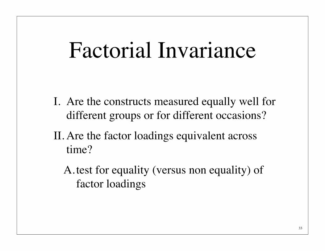
Factorial Invariance

I. Are the constructs measured equally well for different groups or for different occasions?

II. Are the factor loadings equivalent across time?

A. test for equality (versus non equality) of factor loadings

33

specify equality

constraints

path label initial estimate [1,] "Induction -> Induct1" NA "1" [2,] "Induction -> Induct2" "2" NA [3,] "Induction -> Induct3" "3" NA [4,] "Figural -> Figural1" NA "1" [5,] "Figural -> Figural2" "5" NA [6,] "Figural -> Figural3" "6" NA [7,] "Figural.time2 -> Fig2.1" NA "1" [8,] "Figural.time2 -> Fig2.2" "5" NA [9,] "Figural.time2 -> Fig2.3" "6" NA [10,] "Induction -> Figural" "i" NA [11,] "Induction -> Figural.time2" "j" NA [12,] "Figural -> Figural.time2" "k" NA [13,] "Figural3 <-> Fig2.3" "10" NA [14,] "Induct1 <-> Induct1" "u" NA [15,] "Induct2 <-> Induct2" "v" NA [16,] "Induct3 <-> Induct3" "w" NA [17,] "Figural1 <-> Figural1" "x" NA [18,] "Figural2 <-> Figural2" "y" NA [19,] "Figural3 <-> Figural3" "z" NA [20,] "Fig2.1 <-> Fig2.1" "q" NA [21,] "Fig2.2 <-> Fig2.2" "r" NA [22,] "Fig2.3 <-> Fig2.3" "s" NA [23,] "Induction <-> Induction" "A" "1" [24,] "Figural <-> Figural" "B" "1" [25,] "Figural.time2 <-> Figural.time2" "C" "1"

Test the modelcompare fits

sem.prob5e <- sem(model.prob5e,prob5,220)> summary(sem.prob5e,digits=2)

Model Chisquare = 21 Df = 25 Pr(>Chisq) = 0.7 Chisquare (null model) = 1177 Df = 36 Goodness-of-fit index = 0.98 Adjusted goodness-of-fit index = 0.96 RMSEA index = 0 90% CI: (NA, 0.043) Bentler-Bonnett NFI = 0.98 Tucker-Lewis NNFI = 1 Bentler CFI = 1 BIC = -114

Equality

Model: Factors are different

Model Chisquare = 21 Df = 23 Pr(>Chisq) = 0.61 Chisquare (null model) = 1177 Df = 36 Goodness-of-fit index = 0.98 Adjusted goodness-of-fit index = 0.96 RMSEA index = 0 90% CI: (NA, 0.049) Bentler-Bonnett NFI = 0.98 Tucker-Lewis NNFI = 1 Bentler CFI = 1 BIC = -104

Chi square is not noticeably better but use up 2 df

Sensitivity to size Model Chisquare = 191.11 Df = 25 Pr(>Chisq) = 0 Chisquare (null model) = 10747 Df = 36 Goodness-of-fit index = 0.9798 Adjusted goodness-of-fit index = 0.96365 RMSEA index = 0.057652 90% CI: (0.050178, 0.065419) Bentler-Bonnett NFI = 0.98222 Tucker-Lewis NNFI = 0.97767 Bentler CFI = 0.9845 BIC = 1.084

Pretend we have 2000 participants

What do we mean when we fit a model?

I. Special issue of Personality and Individual Difference devoted to this topic

A.Barratt, P. (2007) Structural equation modelling: Adjudging model fit. Personality and individual differences, 815-824.B. http://www.sciencedirect.com/science/journal/01918869

II. Paul Barratt: Target articleA. replies by Bentler, Steiger, Mulaik

38