Embed Size (px)
Citation preview

Linear Regression Analysis
Theory and Computing

This page intentionally left blankThis page intentionally left blank

Linear
Regression Analysis
Theory and Computing
Xin YanUniversity of Missouri–Kansas City, USA
Xiao Gang SuUniversity of Central Florida, USA
World Scientific
NEW JERSEY . LONDON . SINGAPORE . BEIJING . SHANGHAI . HONG KONG . TAIPEI . CHENNAI

Library of Congress Cataloging-in-Publication DataYan, Xin
Linear regression analysis : theory and computing / by Xin Yan & Xiaogang Su.p. cm.
Includes bibliographical references and index.ISBN-13: 978-981-283-410-2 (hardcover : alk. paper)ISBN-10: 981-283-410-9 (hardcover : alk. paper)
1. Regression analysis. I. Su, Xiaogang II. Title.QA278.2.Y36 2009519.5'36--dc22
2009012000
British Library Cataloguing-in-Publication DataA catalogue record for this book is available from the British Library.
For photocopying of material in this volume, please pay a copying fee through the CopyrightClearance Center, Inc., 222 Rosewood Drive, Danvers, MA 01923, USA. In this case permission tophotocopy is not required from the publisher.
All rights reserved. This book, or parts thereof, may not be reproduced in any form or by any means,electronic or mechanical, including photocopying, recording or any information storage and retrievalsystem now known or to be invented, without written permission from the Publisher.
Copyright © 2009 by World Scientific Publishing Co. Pte. Ltd.
Published by
World Scientific Publishing Co. Pte. Ltd.
5 Toh Tuck Link, Singapore 596224
USA office: 27 Warren Street, Suite 401-402, Hackensack, NJ 07601
UK office: 57 Shelton Street, Covent Garden, London WC2H 9HE
Printed in Singapore.
EH - Linear Regression.pmd 5/8/2009, 12:11 PM1

April 29, 2009 11:50 World Scientific Book - 9in x 6in Regression˙master
Preface
In statistics, regression analysis consists of techniques for modeling therelationship between a dependent variable (also called response variable)and one or more independent variables (also known as explanatory vari-ables or predictors). In regression, the dependent variable is modeled asa function of independent variables, corresponding regression parameters(coefficients), and a random error term which represents variation in thedependent variable unexplained by the function of the dependent variablesand coefficients. In linear regression the dependent variable is modeled asa linear function of a set of regression parameters and a random error. Theparameters need to be estimated so that the model gives the “ best fit ”to the data. The parameters are estimated based on predefined criterion.The most commonly used criterion is the least squares method, but othercriteria have also been used that will result in different estimators of theregression parameters. The statistical properties of the estimator derivedusing different criteria will be different from the estimator using the leastsquares principle. In this book the least squares principle will be utilizedto derive estimates of the regression parameters. If a regression model ad-equately reflects the true relationship between the response variable andindependent variables, this model can be used for predicting dependentvariable, identifying important independent variables, and establishing de-sired causal relationship between the response variable and independentvariables.
To perform regression analysis, an investigator often assembles data on un-derlying variables of interest and employs regression model to estimate thequantitative causal effect of the independent variables to the response vari-able. The investigator also typically assesses the “ statistical significance ”of the estimated relationship between the independent variables and depen-
v
April 29, 2009 11:50 World Scientific Book - 9in x 6in Regression˙master
vi Linear Regression Analysis: Theory and Computing
dent variable, that is, the degree of confidence on how the true relationshipis close to the estimated statistical relationship.
Regression analysis is a process used to estimate a function which predictsvalue of response variable in terms of values of other independent variables.If the regression function is determined only through a set of parametersthe type of regression is the parametric regression. Many methods havebeen developed to determine various parametric relationships between re-sponse variable and independent variables. These methods typically dependon the form of parametric regression function and the distribution of theerror term in a regression model. For example, linear regression, logisticregression, Poisson regression, and probit regression, etc. These particu-lar regression models assume different regression functions and error termsfrom corresponding underline distributions. A generalization of linear re-gression models has been formalized in the “ generalized linear model ”and it requires to specify a link function which provides the relationshipbetween the linear predictor and the mean of the distribution function.
The regression model often relies heavily on the underlying assumptionsbeing satisfied. Regression analysis has been criticized as being misused forthese purposes in many cases where the appropriate assumptions cannotbe verified to hold. One important factor for such criticism is due to thefact that a regression model is easier to be criticized than to find a methodto fit a regression model (Cook and Weisberg (1982)). However, checkingmodel assumptions should never be oversighted in regression analysis.
By saying much about regression model we would like to go back to thepurpose of this book. The goal of the book is to provide a comprehensive,one-semester textbook in the area of regression analysis. The book includescarefully selected topics and will not assume to serve as a complete refer-ence book in the area of regression analysis, but rather as an easy-to-readtextbook to provide readers, particularly the graduate students majoringin either statistics or biostatistics, or those who use regression analysissubstantially in their subject fields, the fundamental theories on regressionanalysis, methods for regression model diagnosis, and computing techniquesin regression. In addition to carefully selected classical topics for regressionanalysis, we also include some recent developments in the area of regres-sion analysis such as the least absolute shrinkage and selection operator(LASSO) proposed by Tibshirani (1996) and Bayes averaging method.

April 29, 2009 11:50 World Scientific Book - 9in x 6in Regression˙master
Preface vii
The topics on regression analysis covered in this book are distributed among9 chapters. Chapter 1 briefly introduces the basic concept of regression anddefines the linear regression model. Chapters 2 and 3 cover the simple linearregression and multiple linear regression. Although the simple linear regres-sion is a special case of the multiple linear regression, we present it withoutusing matrix and give detailed derivations that highlight the fundamentalconcepts in linear regression. The presentation of multiple regression fo-cus on the concept of vector space, linear projection, and linear hypothesistest. The theory of matrix is used extensively for the proofs of the statisti-cal properties of linear regression model. Chapters 4 through 6 discuss thediagnosis of linear regression model. These chapters cover outlier detection,influential observations identification, collinearity, confounding, regressionon dummy variables, checking for equal variance assumption, graphical dis-play of residual diagnosis, and variable transformation technique in linearregression analysis. Chapters 7 and 8 provide further discussions on thegeneralizations of the ordinary least squares estimation in linear regres-sion. In these two chapters we discuss how to extend the regression modelto situation where the equal variance assumption on the error term fails.To model the regression data with unequal variance the generalized leastsquares method is introduced. In Chapter 7, two shrinkage estimators, theridge regression and the LASSO are introduced and discussed. A brief dis-cussion on the least squares method for nonlinear regression is also included.Chapter 8 briefly introduces the generalized linear models. In particular,the Poisson Regression for count data and the logistic regression for binarydata are discussed. Chapter 9 briefly discussed the Bayesian linear regres-sion models. The Bayes averaging method is introduced and discussed.
The purpose of including these topics in the book is to foster a better un-derstanding of regression modeling. Although these topics and techniquesare presented largely for regression, the ideas behind these topics and thetechniques are also applicable in other areas of statistical modeling. Thetopics presented in the book cover fundamental theories in linear regres-sion analysis and we think that they are the most useful and relevant tothe future research into this area. A thorough understanding of the basictheories, model diagnosis, and computing techniques in linear regressionanalysis is necessary for those who would like to learn statistics either asa discipline or as a substantial tool in their subject field. To this end,we provide detailed proofs of fundamental theories related to linear regres-sion modeling, diagnosis, and computing so that readers can understand

April 29, 2009 11:50 World Scientific Book - 9in x 6in Regression˙master
viii Linear Regression Analysis: Theory and Computing
the methods in regression analysis and actually model the data using themethods presented in the book.
To enable the book serves the intended purpose as a graduate textbookfor regression analysis, in addition to detailed proofs, we also include manyexamples to illustrate relevant computing techniques in regression analysisand diagnosis. We hope that this would increase the readability and helpto understand the regression methods for students who expect a thoroughunderstanding of regression methods and know how to use these methodsto solve for practical problems. In addition, we tried to avoid an oversized-textbook so that it can be taught in one semester. We do not intend to writea complete reference book for regression analysis because it will require asignificantly larger volume of the book and may not be suitable for a text-book of regression course. In our practice we realize that graduate studentsoften feel overwhelming when try to read an oversized textbook. There-fore, we focus on presenting fundamental theories and detailed derivationsthat can highlight the most important methods and techniques in linearregression analysis.
Most computational examples of regression analysis and diagnosis in thebook use one of popular software package the Statistical Analysis System(SAS), although readers are not discouraged to use other statistical softwarepackages in their subject area. Including illustrative SAS programs for theregression analysis and diagnosis in the book is to help readers to becomefamiliar with various computing techniques that are necessary to regressionanalysis. In addition, the SAS Output Delivery System (ODS) is introducedto enable readers to generate output tables and figures in a desired format.These illustrative programs are often arranged in the end of each chapterwith brief explanations. In addition to the SAS, we also briefly introducethe software R which is a freeware. R has many user-written functions forimplementation of various statistical methods including regression. Thesefunctions are similar to the built-in functions in the commercial softwarepackage S-PLUS. We provide some programs in R to produce desired re-gression diagnosis graphs. Readers are encouraged to learn how to use thesoftware R to perform regression analysis, diagnosis, and producing graphs.
X. Yan and X. G. Su

April 29, 2009 11:50 World Scientific Book - 9in x 6in Regression˙master
Contents
Preface v
List of Figures xv
List of Tables xvii
1. Introduction 1
1.1 Regression Model . . . . . . . . . . . . . . . . . . . . . . . 11.2 Goals of Regression Analysis . . . . . . . . . . . . . . . . 41.3 Statistical Computing in Regression Analysis . . . . . . . 5
2. Simple Linear Regression 9
2.1 Introduction . . . . . . . . . . . . . . . . . . . . . . . . . . 92.2 Least Squares Estimation . . . . . . . . . . . . . . . . . . 102.3 Statistical Properties of the Least Squares Estimation . . 132.4 Maximum Likelihood Estimation . . . . . . . . . . . . . . 182.5 Confidence Interval on Regression Mean and Regression
Prediction . . . . . . . . . . . . . . . . . . . . . . . . . . . 192.6 Statistical Inference on Regression Parameters . . . . . . 212.7 Residual Analysis and Model Diagnosis . . . . . . . . . . 252.8 Example . . . . . . . . . . . . . . . . . . . . . . . . . . . . 28
3. Multiple Linear Regression 41
3.1 Vector Space and Projection . . . . . . . . . . . . . . . . . 413.1.1 Vector Space . . . . . . . . . . . . . . . . . . . . . 413.1.2 Linearly Independent Vectors . . . . . . . . . . . 443.1.3 Dot Product and Projection . . . . . . . . . . . . 44
ix

May 7, 2009 10:22 World Scientific Book - 9in x 6in Regression˙master
x Linear Regression Analysis: Theory and Computing
3.2 Matrix Form of Multiple Linear Regression . . . . . . . . 483.3 Quadratic Form of Random Variables . . . . . . . . . . . 493.4 Idempotent Matrices . . . . . . . . . . . . . . . . . . . . . 503.5 Multivariate Normal Distribution . . . . . . . . . . . . . . 543.6 Quadratic Form of the Multivariate Normal Variables . . 563.7 Least Squares Estimates of the Multiple Regression
Parameters . . . . . . . . . . . . . . . . . . . . . . . . . . 583.8 Matrix Form of the Simple Linear Regression . . . . . . . 623.9 Test for Full Model and Reduced Model . . . . . . . . . . 643.10 Test for General Linear Hypothesis . . . . . . . . . . . . . 663.11 The Least Squares Estimates of Multiple Regression
Parameters Under Linear Restrictions . . . . . . . . . . . 673.12 Confidence Intervals of Mean and Prediction in Multiple
Regression . . . . . . . . . . . . . . . . . . . . . . . . . . . 693.13 Simultaneous Test for Regression Parameters . . . . . . . 703.14 Bonferroni Confidence Region for Regression Parameters . 713.15 Interaction and Confounding . . . . . . . . . . . . . . . . 72
3.15.1 Interaction . . . . . . . . . . . . . . . . . . . . . . 733.15.2 Confounding . . . . . . . . . . . . . . . . . . . . . 75
3.16 Regression with Dummy Variables . . . . . . . . . . . . . 773.17 Collinearity in Multiple Linear Regression . . . . . . . . . 81
3.17.1 Collinearity . . . . . . . . . . . . . . . . . . . . . . 813.17.2 Variance Inflation . . . . . . . . . . . . . . . . . . 85
3.18 Linear Model in Centered Form . . . . . . . . . . . . . . . 873.19 Numerical Computation of LSE via QR Decomposition . 92
3.19.1 Orthogonalization . . . . . . . . . . . . . . . . . . 923.19.2 QR Decomposition and LSE . . . . . . . . . . . . 94
3.20 Analysis of Regression Residual . . . . . . . . . . . . . . . 963.20.1 Purpose of the Residual Analysis . . . . . . . . . 963.20.2 Residual Plot . . . . . . . . . . . . . . . . . . . . 973.20.3 Studentized Residuals . . . . . . . . . . . . . . . . 1033.20.4 PRESS Residual . . . . . . . . . . . . . . . . . . . 1033.20.5 Identify Outlier Using PRESS Residual . . . . . . 1063.20.6 Test for Mean Shift Outlier . . . . . . . . . . . . . 108
3.21 Check for Normality of the Error Term in MultipleRegression . . . . . . . . . . . . . . . . . . . . . . . . . . . 115
3.22 Example . . . . . . . . . . . . . . . . . . . . . . . . . . . . 115

May 8, 2009 15:56 World Scientific Book - 9in x 6in Regression˙master
Contents xi
4. Detection of Outliers and Influential Observations
in Multiple Linear Regression 129
4.1 Model Diagnosis for Multiple Linear Regression . . . . . . 130
4.1.1 Simple Criteria for Model Comparison . . . . . . 130
4.1.2 Bias in Error Estimate from Under-specified Model 131
4.1.3 Cross Validation . . . . . . . . . . . . . . . . . . . 132
4.2 Detection of Outliers in Multiple Linear Regression . . . . 133
4.3 Detection of Influential Observations in Multiple Linear
Regression . . . . . . . . . . . . . . . . . . . . . . . . . . . 134
4.3.1 Influential Observation . . . . . . . . . . . . . . . 134
4.3.2 Notes on Outlier and Influential Observation . . . 136
4.3.3 Residual Mean Square Error for Over-fitted
Regression Model . . . . . . . . . . . . . . . . . . 137
4.4 Test for Mean-shift Outliers . . . . . . . . . . . . . . . . . 139
4.5 Graphical Display of Regression Diagnosis . . . . . . . . . 142
4.5.1 Partial Residual Plot . . . . . . . . . . . . . . . . 142
4.5.2 Component-plus-residual Plot . . . . . . . . . . . 146
4.5.3 Augmented Partial Residual Plot . . . . . . . . . 147
4.6 Test for Inferential Observations . . . . . . . . . . . . . . 147
4.7 Example . . . . . . . . . . . . . . . . . . . . . . . . . . . . 150
5. Model Selection 157
5.1 Effect of Underfitting and Overfitting . . . . . . . . . . . 157
5.2 All Possible Regressions . . . . . . . . . . . . . . . . . . . 165
5.2.1 Some Naive Criteria . . . . . . . . . . . . . . . . 165
5.2.2 PRESS and GCV . . . . . . . . . . . . . . . . . . 166
5.2.3 Mallow’s CP . . . . . . . . . . . . . . . . . . . . . 167
5.2.4 AIC, AICC , and BIC . . . . . . . . . . . . . . . . 169
5.3 Stepwise Selection . . . . . . . . . . . . . . . . . . . . . . 171
5.3.1 Backward Elimination . . . . . . . . . . . . . . . . 171
5.3.2 Forward Addition . . . . . . . . . . . . . . . . . . 172
5.3.3 Stepwise Search . . . . . . . . . . . . . . . . . . . 172
5.4 Examples . . . . . . . . . . . . . . . . . . . . . . . . . . . 173
5.5 Other Related Issues . . . . . . . . . . . . . . . . . . . . 179
5.5.1 Variance Importance or Relevance . . . . . . . . 180
5.5.2 PCA and SIR . . . . . . . . . . . . . . . . . . . . 186

May 7, 2009 10:22 World Scientific Book - 9in x 6in Regression˙master
xii Linear Regression Analysis: Theory and Computing
6. Model Diagnostics 195
6.1 Test Heteroscedasticity . . . . . . . . . . . . . . . . . . . . 1976.1.1 Heteroscedasticity . . . . . . . . . . . . . . . . . . 1976.1.2 Likelihood Ratio Test, Wald, and Lagrange Multi-
plier Test . . . . . . . . . . . . . . . . . . . . . . . 1986.1.3 Tests for Heteroscedasticity . . . . . . . . . . . . . 201
6.2 Detection of Regression Functional Form . . . . . . . . . . 2046.2.1 Box-Cox Power Transformation . . . . . . . . . . 2056.2.2 Additive Models . . . . . . . . . . . . . . . . . . . 2076.2.3 ACE and AVAS . . . . . . . . . . . . . . . . . . . 2106.2.4 Example . . . . . . . . . . . . . . . . . . . . . . . 211
7. Extensions of Least Squares 219
7.1 Non-Full-Rank Linear Regression Models . . . . . . . . . 2197.1.1 Generalized Inverse . . . . . . . . . . . . . . . . . 2217.1.2 Statistical Inference on Null-Full-Rank Regression
Models . . . . . . . . . . . . . . . . . . . . . . . . 2237.2 Generalized Least Squares . . . . . . . . . . . . . . . . . . 229
7.2.1 Estimation of (β, σ2) . . . . . . . . . . . . . . . . 2307.2.2 Statistical Inference . . . . . . . . . . . . . . . . . 2317.2.3 Misspecification of the Error Variance Structure . 2327.2.4 Typical Error Variance Structures . . . . . . . . 2337.2.5 Example . . . . . . . . . . . . . . . . . . . . . . . 236
7.3 Ridge Regression and LASSO . . . . . . . . . . . . . . . . 2387.3.1 Ridge Shrinkage Estimator . . . . . . . . . . . . . 2397.3.2 Connection with PCA . . . . . . . . . . . . . . . 2437.3.3 LASSO and Other Extensions . . . . . . . . . . . 2467.3.4 Example . . . . . . . . . . . . . . . . . . . . . . . 250
7.4 Parametric Nonlinear Regression . . . . . . . . . . . . . . 2597.4.1 Least Squares Estimation in Nonlinear Regression 2617.4.2 Example . . . . . . . . . . . . . . . . . . . . . . . 263
8. Generalized Linear Models 269
8.1 Introduction: A Motivating Example . . . . . . . . . . . . 2698.2 Components of GLM . . . . . . . . . . . . . . . . . . . . 272
8.2.1 Exponential Family . . . . . . . . . . . . . . . . . 2728.2.2 Linear Predictor and Link Functions . . . . . . . 273
8.3 Maximum Likelihood Estimation of GLM . . . . . . . . . 274

May 7, 2009 10:22 World Scientific Book - 9in x 6in Regression˙master
Contents xiii
8.3.1 Likelihood Equations . . . . . . . . . . . . . . . . 2748.3.2 Fisher’s Information Matrix . . . . . . . . . . . . 2758.3.3 Optimization of the Likelihood . . . . . . . . . . . 276
8.4 Statistical Inference and Other Issues in GLM . . . . . . 2788.4.1 Wald, Likelihood Ratio, and Score Test . . . . . 2788.4.2 Other Model Fitting Issues . . . . . . . . . . . . 281
8.5 Logistic Regression for Binary Data . . . . . . . . . . . . 2828.5.1 Interpreting the Logistic Model . . . . . . . . . . 2828.5.2 Estimation of the Logistic Model . . . . . . . . . 2848.5.3 Example . . . . . . . . . . . . . . . . . . . . . . . 285
8.6 Poisson Regression for Count Data . . . . . . . . . . . . 2878.6.1 The Loglinear Model . . . . . . . . . . . . . . . . 2878.6.2 Example . . . . . . . . . . . . . . . . . . . . . . . 288
9. Bayesian Linear Regression 297
9.1 Bayesian Linear Models . . . . . . . . . . . . . . . . . . . 2979.1.1 Bayesian Inference in General . . . . . . . . . . . 2979.1.2 Conjugate Normal-Gamma Priors . . . . . . . . . 2999.1.3 Inference in Bayesian Linear Model . . . . . . . . 3029.1.4 Bayesian Inference via MCMC . . . . . . . . . . . 3039.1.5 Prediction . . . . . . . . . . . . . . . . . . . . . . 3069.1.6 Example . . . . . . . . . . . . . . . . . . . . . . . 307
9.2 Bayesian Model Averaging . . . . . . . . . . . . . . . . . 309
Bibliography 317
Index 325

April 29, 2009 11:50 World Scientific Book - 9in x 6in Regression˙master
This page intentionally left blankThis page intentionally left blank
April 29, 2009 11:50 World Scientific Book - 9in x 6in Regression˙master
List of Figures
2.1 (a) Regression Line and Scatter Plot. (b) Residual Plot, (c)95% Confidence Band for Regression Mean. (d) 95% ConfidenceBand for Regression Prediction. . . . . . . . . . . . . . . . . . . 33
2.2 Q-Q Plot for Regression Model density=β0 + β1 stiffness + ε . 34
3.1 Response Curves of Y Versus X1 at Different Values of X2 inModels (3.33) and (3.32). . . . . . . . . . . . . . . . . . . . . . 74
3.2 Regression on Dummy Variables . . . . . . . . . . . . . . . . . 823.3 Various Shapes of Residual Plots . . . . . . . . . . . . . . . . . 983.4 Residual Plots of the Regression Model of the US Population . 100
4.1 Partial Residual Plots for Regression Models . . . . . . . . . . 145
5.1 (a) Plot of the Average and Standard Deviation of SSPE Pre-diction from 100 Simulation Runs; (b) A Hypothetical Plot ofPrediction Error Versus Model Complexity in General Regres-sion Problems. . . . . . . . . . . . . . . . . . . . . . . . . . . . 163
5.2 Variable Importance for the Quasar Data: Random Forestsvs. RELIEF. . . . . . . . . . . . . . . . . . . . . . . . . . . . . 181
5.3 A Simulation Example on Variable Importance: RandomForests vs. RELIEF. . . . . . . . . . . . . . . . . . . . . . . . . 185
6.1 Box-Cox Power Transformation of Y in the Navy ManpowerData: Plot of the Log-likelihood Score vs. λ. . . . . . . . . . . 212
6.2 Detecting the Nonlinear Effect of x1 and x2 via Additive Modelsin the Navy Manpower Data. . . . . . . . . . . . . . . . . . . . 213
6.3 AVAS Results for the Navy Manpower Data: (a) Plot of g(Y );(b) Plot of f1(X1); (c) Plot of f2(X2). . . . . . . . . . . . . . . 214
xv
April 29, 2009 11:50 World Scientific Book - 9in x 6in Regression˙master
xvi Linear Regression Analysis: Theory and Computing
6.4 AVAS Results for the Navy Manpower Data: (a) 3-D Scat-ter Plot of the Original Data; (b) 3-D Scatter Plot of g(Y )vs. f1(X1) and f2(X2) after Transformation. . . . . . . . . . . 215
7.1 (a) The Scatter Plot of DBP Versus Age; (b) Residual ver-sus Age; (c) Absolute Values of Residuals |εi| Versus Age; (d)Squared Residuals ε2
i Versus Age. . . . . . . . . . . . . . . . . . 2377.2 Estimation in Constrained Least Squares in the Two-
dimensional Case: Contours of the Residual Sum of Squares andthe Constraint Functions in (a) Ridge Regression; (b) LASSO. 240
7.3 Paired Scatter Plots for Longley’s (1967) Economic Data. . . . 2517.4 Ridge Regression for Longley’s (1967) Economic Data: (a) Plot
of Parameter Estimates Versus s; (b) Plot of GCV Values Versus s.2547.5 LASSO Procedure for Longley’s (1967) Economic Data: (a) Plot
of Standardized Parameter Estimates Versus Fraction of the L1
Shrinkage; (b) Plot of Cross-validated SSE Versus Fraction. . . 2577.6 Plot of the Logistic Function With C = 1: (a) When B Varies
With A = 1; (b) When A Varies With B = 1. . . . . . . . . . . 2607.7 Parametric Nonlinear Regression with the US Population
Growth Data Reproduced from Fox (2002): (a) Scatter Plotof the Data Superimposed by the LS Fitted Straight Line; (b)Plot of the Residuals From the Linear Model Versus Year; (c)Scatter Plot of the Data Superimposed by the Fitted NonlinearCurve; (d) Plot of the Residuals From the Nonlinear Fit VersusYear. . . . . . . . . . . . . . . . . . . . . . . . . . . . . . . . . . 264
8.1 (a) Scatterplot of the CHD Data, Superimposed With theStraight Line from Least Squares Fit; (b) Plot of the Percentageof Subjects With CHD Within Each Age Group, Superimposedby LOWESS Smoothed Curve. . . . . . . . . . . . . . . . . . . 270
8.2 Plot of the Log-likelihood Function: Comparison of Wald, LRT,and Score Tests on H0 : β = b. . . . . . . . . . . . . . . . . . . 280
9.1 Posterior Marginal Densities of (β, σ2): Bayesian Linear Regres-sion for Shingle Data. . . . . . . . . . . . . . . . . . . . . . . . 308
9.2 Posterior Densities for Predicting yp: the Shingle Data. . . . . 3099.3 The 13 Selected Models by BMA: the Quasar Data. . . . . . . 3139.4 Posterior Distributions of the Coefficients Generated by BMA:
the Quasar Data. . . . . . . . . . . . . . . . . . . . . . . . . . . 314

April 29, 2009 11:50 World Scientific Book - 9in x 6in Regression˙master
List of Tables
1.1 Smoking and Mortality Data . . . . . . . . . . . . . . . . . . . 1
2.1 Parent’s Height and Children’s Height . . . . . . . . . . . . . . 92.2 Degrees of Freedom in Partition of Total Variance . . . . . . . 222.3 Distributions of Partition of Total Variance . . . . . . . . . . . 232.4 ANOVA Table 1 . . . . . . . . . . . . . . . . . . . . . . . . . . 232.5 Confidence Intervals on Parameter Estimates . . . . . . . . . . 292.6 ANOVA Table 2 . . . . . . . . . . . . . . . . . . . . . . . . . . 302.7 Regression Table . . . . . . . . . . . . . . . . . . . . . . . . . . 302.8 Parameter Estimates of Simple Linear Regression . . . . . . . . 302.9 Table for Fitted Values and Residuals . . . . . . . . . . . . . . 312.10 Data for Two Parallel Regression Lines . . . . . . . . . . . . . 362.11 Chemical Reaction Data . . . . . . . . . . . . . . . . . . . . . 382.12 Weight-lifting Test Data . . . . . . . . . . . . . . . . . . . . . . 39
3.1 Two Independent Vectors . . . . . . . . . . . . . . . . . . . . . 833.2 Two Highly Correlated Vectors . . . . . . . . . . . . . . . . . . 833.3 Correlation Matrix for Variables x1, x2, · · · , x5 . . . . . . . . . 883.4 Parameter Estimates and Variance Inflation . . . . . . . . . . . 883.5 Correlation Matrix after Deleting Variable x1 . . . . . . . . . . 883.6 Variance Inflation after Deleting x1 . . . . . . . . . . . . . . . . 883.7 United States Population Data (in Millions) . . . . . . . . . . . 973.8 Parameter Estimates for Model Population=Year . . . . . . . . 993.9 Parameter Estimates for Model Population=Year+Year2 . . . . 993.10 Parameter Estimates for Regression Model Population=β0 +β1
Year+ β2 Year2+z . . . . . . . . . . . . . . . . . . . . . . . . . 1013.11 Coal-cleansing Data . . . . . . . . . . . . . . . . . . . . . . . . 109
xvii

April 29, 2009 11:50 World Scientific Book - 9in x 6in Regression˙master
xviii Linear Regression Analysis: Theory and Computing
3.12 Parameter Estimates for Regression Model for Coal-CleansingData . . . . . . . . . . . . . . . . . . . . . . . . . . . . . . . . . 109
3.13 Residuals . . . . . . . . . . . . . . . . . . . . . . . . . . . . . . 1103.14 Manpower Data . . . . . . . . . . . . . . . . . . . . . . . . . . 1113.15 Simultaneous Outlier Detection . . . . . . . . . . . . . . . . . . 1133.16 Detection of Multiple Mean Shift Outliers . . . . . . . . . . . . 1143.17 Stand Characteristics of Pine Tree Data . . . . . . . . . . . . . 1163.18 Parameter Estimates and Confidence Intervals Using x1, x2 and
x3 . . . . . . . . . . . . . . . . . . . . . . . . . . . . . . . . . . 1173.19 Parameter Estimates and Confidence Intervals after Deleting x3 1173.20 Confidence Intervals on Regression Mean and Prediction With-
out Deletion . . . . . . . . . . . . . . . . . . . . . . . . . . . . . 1183.21 Confidence Intervals on Regression Mean and Prediction After
Deleting x3 . . . . . . . . . . . . . . . . . . . . . . . . . . . . . 1183.22 Regression Model for Centralized Data . . . . . . . . . . . . . . 1193.23 Test for Equal Slope Among 3 Groups . . . . . . . . . . . . . . 1213.24 Regression by Group . . . . . . . . . . . . . . . . . . . . . . . . 1213.25 Data Set for Calculation of Confidence Interval on Regression
Prediction . . . . . . . . . . . . . . . . . . . . . . . . . . . . . . 1233.26 Propellant Grain Data . . . . . . . . . . . . . . . . . . . . . . . 1243.27 Data Set for Testing Linear Hypothesis . . . . . . . . . . . . . 1243.28 Algae Data . . . . . . . . . . . . . . . . . . . . . . . . . . . . . 126
4.1 Coal-cleansing Data . . . . . . . . . . . . . . . . . . . . . . . . 1414.2 Parameter Estimates for y = b0 + b1x1 + b2x2 + b3x3 . . . . . . 1414.3 Residuals, Leverage, and ti . . . . . . . . . . . . . . . . . . . . 1424.4 Navy Manpower Data . . . . . . . . . . . . . . . . . . . . . . . 1444.5 Residuals for Model With Regressors x1 and x2 . . . . . . . . . 1464.6 Residuals for Model With Regressors x
131 and x2 . . . . . . . . 146
4.7 Sales Data for Asphalt Shingles . . . . . . . . . . . . . . . . . . 1514.8 Values of PRESS Statistic for Various Regression Models . . . 1524.9 PRESS Residuals and Leverages for Models Including x1, x2
(press12, h12) and Including x1, x2, x3 (press123, h123) . . . . 1534.10 Data Set for Multiple Mean Shift Outliers . . . . . . . . . . . 1544.11 Fish Biomass Data . . . . . . . . . . . . . . . . . . . . . . . . . 155
5.1 The Quasar Data from Ex. 4.9 in Mendenhall and Sinich (2003) 1745.2 All Possible Regression Selection for the Quasar Data. . . . . . 1755.3 Backward Elimination Procedure for the Quasar Data. . . . . . 190

April 29, 2009 11:50 World Scientific Book - 9in x 6in Regression˙master
List of Tables xix
5.4 Forward Addition Procedure for the Quasar Data. . . . . . . . 1915.5 The Clerical Data from Ex. 6.4 in Mendenhall and Sinich (2003) 1925.6 Backward Elimination Results for the Clerical Data. . . . . . . 1935.7 Results of a Simulated Example for Inspecting Overall Signifi-
cance in Stepwise Selection . . . . . . . . . . . . . . . . . . . . 1935.8 Female Teachers Effectiveness Data . . . . . . . . . . . . . . . . 1945.9 All-subset-regression for Female Teacher Effectiveness Data . . 194
6.1 Results of Efficiency Tests . . . . . . . . . . . . . . . . . . . . . 216
7.1 Layouts for Data Collected in One-way ANOVA Experiments. 2207.2 Analysis of the Diastolic Blood Pressure Data: (a) Ordinary
Least Squares (OLS) Estimates; (b) Weighted Least Squares(WLS) Fitting with Weights Derived from Regressing AbsoluteValues |εi| of the Residuals On Age. . . . . . . . . . . . . . . . 238
7.3 The Macroeconomic Data Set in Longley (1967). . . . . . . . . 2497.4 Variable Description for Longley’s (1967) Macroeconomic Data. 2507.5 Least Squares Results for Longley’s (1967) Economic Data. . . 2527.6 Ridge Regression and LASSO for Longley’s (1967) Data. . . . . 2557.7 Nonlinear Regression Results of the US Population Data from
PROC NLIN and PROC AUTOREG. . . . . . . . . . . . . . . 265
8.1 Frequency Table of AGE Group by CHD. . . . . . . . . . . . . 2718.2 Variable Description for the Kyphosis Data: Logistic Regression
Example. . . . . . . . . . . . . . . . . . . . . . . . . . . . . . . 2858.3 Analysis Results for the Kyphosis Data from PROC LOGISTIC. 2868.4 Variable Description for the Log-Linear Regression Example. . 2888.5 Analysis Results for the School Absence Data from PROC GEN-
MOD. . . . . . . . . . . . . . . . . . . . . . . . . . . . . . . . . 2908.6 Variable Description for the Prostate Cancer Data. . . . . . . . 2938.7 Table of Parameter Estimates and the Estimated Covariance
Matrix for Model I: the Prostate Cancer Data. . . . . . . . . . 2948.8 Table of Parameter Estimates and the Estimated Covariance
Matrix for Model II: the Prostate Cancer Data. 2958.9 The Maximized Loglikelihood Scores for Several Fitted Models
with the Prostate Cancer Data. . . . . . . . . . . . . . . . . . 295
9.1 Bayesian Linear Regression Results With the Shingle Data. . . 3079.2 BMA Results for the Quasar Data. . . . . . . . . . . . . . . . . 315

April 29, 2009 11:50 World Scientific Book - 9in x 6in Regression˙master
This page intentionally left blankThis page intentionally left blank

April 29, 2009 11:50 World Scientific Book - 9in x 6in Regression˙master
Chapter 1
Introduction
1.1 Regression Model
Researchers are often interested in the relationships between one variableand several other variables. For example, does smoking cause lung can-cer? Following Table 1.1 summarizes a study carried out by governmentstatisticians in England. The data concern 25 occupational groups andare condensed from data on thousands of individual men. One variableis smoking ratio which is a measure of the number of cigarettes smokedper day by men in each occupation relative to the number smoked by allmen of the same age. Another variable is the standardized mortality ra-tio. To answer the question that does smoking cause cancer we may liketo know the relationship between the derived mortality ratio and smokingratio. This falls into the scope of regression analysis. Data from a scientific
Table 1.1 Smoking and Mortality Data
Smoking 77 112 137 113 117 110 94 125 116 133Mortality 84 96 116 144 123 139 128 113 155 146
Smoking 102 115 111 105 93 87 88 91 102 100Mortality 101 128 118 115 113 79 104 85 88 120
Smoking 91 76 104 66 107Mortality 104 60 129 51 86
experiment often lead to ask whether there is a causal relationship betweentwo or more variables. Regression analysis is the statistical method forinvestigating such relationship. It is probably one of the oldest topics inthe area of mathematical statistics dating back to about two hundred years
1

April 29, 2009 11:50 World Scientific Book - 9in x 6in Regression˙master
2 Linear Regression Analysis: Theory and Computing
ago. The earliest form of the linear regression was the least squares method,which was published by Legendre in 1805, and by Gauss in 1809. The term“least squares” is from Legendre’s term. Legendre and Gauss both appliedthe method to the problem of determining, from astronomical observations,the orbits of bodies about the sun. Euler had worked on the same problem(1748) without success. Gauss published a further development of the the-ory of least squares in 1821, including a version of the today’s well-knownGauss-Markov theorem, which is a fundamental theorem in the area of thegeneral linear models.
What is a statistical model? A statistical model is a simple description ofa state or process. “A model is neither a hypothesis nor a theory. Unlikescientific hypotheses, a model is not verifiable directly by an experiment.For all models of true or false, the validation of a model is not that it is“true” but that it generates good testable hypotheses relevant to importantproblems.” (R. Levins, Am. Scientist 54: 421-31, 1966)
Linear regression requires that model is linear in regression parameters.Regression analysis is the method to discover the relationship between oneor more response variables (also called dependent variables, explained vari-ables, predicted variables, or regressands, usually denoted by y) and thepredictors (also called independent variables, explanatory variables, con-trol variables, or regressors, usually denoted by x1, x2, · · · , xp).
There are three types of regression. The first is the simple linear regression.The simple linear regression is for modeling the linear relationship betweentwo variables. One of them is the dependent variable y and another isthe independent variable x. For example, the simple linear regression canmodel the relationship between muscle strength (y) and lean body mass(x). The simple regression model is often written as the following form
y = β0 + β1x + ε, (1.1)
where y is the dependent variable, β0 is y intercept, β1 is the gradient orthe slope of the regression line, x is the independent variable, and ε is therandom error. It is usually assumed that error ε is normally distributedwith E(ε) = 0 and a constant variance Var(ε) = σ2 in the simple linearregression.
The second type of regression is the multiple linear regression which is alinear regression model with one dependent variable and more than one
April 29, 2009 11:50 World Scientific Book - 9in x 6in Regression˙master
Introduction 3
independent variables. The multiple linear regression assumes that theresponse variable is a linear function of the model parameters and thereare more than one independent variables in the model. The general formof the multiple linear regression model is as follows:
y = β0 + β1x1 + · · ·+ βpxp + ε, (1.2)
where y is dependent variable, β0, β1, β2, · · · , βp are regression coefficients,and x1, x2, · · · , xn are independent variables in the model. In the classicalregression setting it is usually assumed that the error term ε follows thenormal distribution with E(ε) = 0 and a constant variance Var(ε) = σ2.
Simple linear regression is to investigate the linear relationship between onedependent variable and one independent variable, while the multiple linearregression focuses on the linear relationship between one dependent variableand more than one independent variables. The multiple linear regressioninvolves more issues than the simple linear regression such as collinearity,variance inflation, graphical display of regression diagnosis, and detectionof regression outlier and influential observation.
The third type of regression is nonlinear regression, which assumes thatthe relationship between dependent variable and independent variables isnot linear in regression parameters. Example of nonlinear regression model(growth model) may be written as
y =α
1 + eβt+ ε, (1.3)
where y is the growth of a particular organism as a function of time t, α
and β are model parameters, and ε is the random error. Nonlinear regres-sion model is more complicated than linear regression model in terms ofestimation of model parameters, model selection, model diagnosis, variableselection, outlier detection, or influential observation identification. Gen-eral theory of the nonlinear regression is beyond the scope of this book andwill not be discussed in detail. However, in addition to the linear regressionmodel we will discuss some generalized linear models. In particular, we willintroduce and discuss two important generalized linear models, logistic re-gression model for binary data and log-linear regression model for countdata in Chapter 8.

April 29, 2009 11:50 World Scientific Book - 9in x 6in Regression˙master
4 Linear Regression Analysis: Theory and Computing
1.2 Goals of Regression Analysis
Regression analysis is one of the most commonly used statistical methodsin practice. Applications of regression analysis can be found in many scien-tific fields including medicine, biology, agriculture, economics, engineering,sociology, geology, etc. The purposes of regression analysis are three-folds:
(1) Establish a casual relationship between response variable y and regres-sors x1, x2, · · · , xn.
(2) Predict y based on a set of values of x1, x2, · · · , xn.(3) Screen variables x1, x2, · · · , xn to identify which variables are more im-
portant than others to explain the response variable y so that the causalrelationship can be determined more efficiently and accurately.
An analyst often follows, but not limited, the following procedures inthe regression analysis.
(1) The first and most important step is to understand the real-life problemwhich is often fallen into a specific scientific field. Carefully determinewhether the scientific question falls into scope of regression analysis.
(2) Define a regression model which may be written as
Response variable = a function of regressors + random error,
or simply in a mathematical format
y = f(x1, x2, · · · , xp) + ε.
You may utilize a well-accepted model in a specific scientific field ortry to define your own model based upon a sound scientific judgementby yourself or expert scientists in the subject area. Defining a modelis often a joint effort among statisticians and experts in a scientificdiscipline. Choosing an appropriate model is the first step for statisticalmodeling and often involve further refinement procedures.
(3) Make distributional assumptions on the random error ε in the regressionmodel. These assumptions need to be verified or tested by the datacollected from experiment. The assumptions are often the basis uponwhich the regression model may be solved and statistical inference isdrawn.
(4) Collect data y and x1, x2, · · · , xp. This data collection step usuallyinvolves substantial work that includes, but not limited to, experimen-tal design, sample size determination, database design, data cleaning,
April 29, 2009 11:50 World Scientific Book - 9in x 6in Regression˙master
Introduction 5
and derivations of analysis variables that will be used in the statisticalanalysis. In many real-life applications, this is a crucial step that ofteninvolve significant amount of work.
(5) According to the software used in the analysis, create data sets in anappropriate format that are easy to be read into a chosen software. Inaddition, it often needs to create more specific analysis data sets forplanned or exploratory statistical analysis.
(6) Carefully evaluate whether or not the selected model is appropriate foranswering the desired scientific questions. Various diagnosis methodsmay be used to evaluate the performance of the selected statisticalmodel. It should be kept in mind that the model diagnosis is for thejudgment of whether the selected statistical model is a sound modelthat can answer the desired scientific questions.
(7) If the model is deemed to be appropriate according to a well acceptedmodel diagnosis criteria, it may be used to answer the desired scientificquestions; otherwise, the model is subject to refinement or modifica-tion. Several iterations of model selection, model diagnosis, and modelrefinement may be necessary and very common in practice.
1.3 Statistical Computing in Regression Analysis
After a linear regression model is chosen and a database is created, the nextstep is statistical computing. The purposes of the statistical computing areto solve for the actual model parameters and to conduct model diagnosis.Various user-friendly statistical softwares have been developed to make theregression analysis easier and more efficient.
Statistical Analysis System (SAS) developed by SAS Institute, Inc. is oneof the popular softwares which can be used to perform regression analysis.The SAS System is an integrated system of software products that enablesusers to perform data entry and data management, to produce statisticalgraphics, to conduct wide range of statistical analyses, to retrieve datafrom data warehouse (extract, transform, load) platform, and to providedynamic interface to other software, etc. One great feature of SAS is thatmany standard statistical methods have been integrated into various SASprocedures that enable analysts easily find desired solutions without writingsource code from the original algorithms of statistical methods. The SAS“macro” language allows user to write subroutines to perform particularuser-defined statistical analysis. SAS compiles and runs on UNIX platform

April 29, 2009 11:50 World Scientific Book - 9in x 6in Regression˙master
6 Linear Regression Analysis: Theory and Computing
and Windows operating system.
Software S-PLUS developed by Insightful Inc. is another one of the mostpopular softwares that have been used substantially by analysts in variousscientific fields. This software is a rigorous computing tool covering a broadrange of methods in statistics. Various built-in S-PLUS functions have beendeveloped that enable users to perform statistical analysis and generateanalysis graphics conveniently and efficiently. The S-PLUS offers a widecollection of specialized modules that provide additional functionality to theS-PLUS in areas such as: volatility forecasting, optimization, clinical trialsanalysis, environmental statistics, and spatial data analysis, data mining.In addition, user can write S-PLUS programs or functions using the S-language to perform statistical analysis of specific needs. The S-PLUScompiles and runs on UNIX platform and Windows operating system.
Statistical Package for Social Sciences (SPSS) is also one of the most widelyused softwares for the statistical analysis in the area of social sciences. Itis one of the preferred softwares used by market researchers, health re-searchers, survey companies, government, education researchers, amongothers. In addition to statistical analysis, data management (case selection,file reshaping, creating derived data) and data documentation (a metadatadictionary is stored) are features of the SPSS. Many features of SPSS areaccessible via pull-down menus or can be programmed with a proprietary4GL command syntax language. Additionally, a “macro” language can beused to write command language subroutines to facilitate special needs ofuser-desired statistical analysis.
Another popular software that can be used for various statistical analysesis R. R is a language and environment for statistical computing and graph-ics. It is a GNU project similar to the S language and environment. R canbe considered as a different implementation of S language. There are someimportant differences, but much code written for S language runs unalteredunder R. The S language is often the vehicle of choice for research in sta-tistical methodology, and R provides an open source route to participationin that activity. One of R’s strengths is the ease with which well-designedpublication-quality plots can be produced, including mathematical symbolsand formulae where needed. Great care has been taken over the defaults forthe design choices in graphics, but user retains full control. R is availableas free software under the terms of the Free Software Foundation’s GNUGeneral Public License in source code form. It compiles and runs on a wide

April 29, 2009 11:50 World Scientific Book - 9in x 6in Regression˙master
Introduction 7
variety of UNIX platforms and similar system Linux, as well as Windows.
Regression analysis can be performed using various softwares such as SAS,S-PLUS, R, or SPSS. In this book we choose the software SAS to illustratethe computing techniques in regression analysis and diagnosis. Extensiveexamples are provided in the book to enable readers to become familiarwith regression analysis and diagnosis using SAS. We also provide someexamples of regression graphic plots using the software R. However, readersare not discouraged to use other softwares to perform regression analysisand diagnosis.

April 29, 2009 11:50 World Scientific Book - 9in x 6in Regression˙master
This page intentionally left blankThis page intentionally left blank

April 29, 2009 11:50 World Scientific Book - 9in x 6in Regression˙master
Chapter 2
Simple Linear Regression
2.1 Introduction
The term “regression” and the methods for investigating the relationshipsbetween two variables may date back to about 100 years ago. It was firstintroduced by Francis Galton in 1908, the renowned British biologist, whenhe was engaged in the study of heredity. One of his observations was thatthe children of tall parents to be taller than average but not as tall as theirparents. This “regression toward mediocrity” gave these statistical meth-ods their name. The term regression and its evolution primarily describestatistical relations between variables. In particular, the simple regressionis the regression method to discuss the relationship between one dependentvariable (y) and one independent variable (x). The following classical dataset contains the information of parent’s height and children’s height.
Table 2.1 Parent’s Height and Children’s Height
Parent 64.5 65.5 66.5 67.5 68.5 69.5 70.5 71.5 72.5
Children 65.8 66.7 67.2 67.6 68.2 68.9 69.5 69.9 72.2
The mean height is 68.44 for children and 68.5 for parents. The regressionline for the data of parents and children can be described as
child height = 21.52 + 0.69 parent height.
The simple linear regression model is typically stated in the form
y = β0 + β1x + ε,
where y is the dependent variable, β0 is the y intercept, β1 is the slope ofthe simple linear regression line, x is the independent variable, and ε is the
9
April 29, 2009 11:50 World Scientific Book - 9in x 6in Regression˙master
10 Linear Regression Analysis: Theory and Computing
random error. The dependent variable is also called response variable, andthe independent variable is called explanatory or predictor variable. Anexplanatory variable explains causal changes in the response variables. Amore general presentation of a regression model may be written as
y = E(y) + ε,
where E(y) is the mathematical expectation of the response variable. WhenE(y) is a linear combination of exploratory variables x1, x2, · · · , xk theregression is the linear regression. If k = 1 the regression is the simple linearregression. If E(y) is a nonlinear function of x1, x2, · · · , xk the regressionis nonlinear. The classical assumptions on error term are E(ε) = 0 and aconstant variance Var(ε) = σ2. The typical experiment for the simple linearregression is that we observe n pairs of data (x1, y1), (x2, y2), · · · , (xn, yn)from a scientific experiment, and model in terms of the n pairs of the datacan be written as
yi = β0 + β1xi + εi for i = 1, 2, · · · , n,
with E(εi) = 0, a constant variance Var(εi) = σ2, and all εi’s are indepen-dent. Note that the actual value of σ2 is usually unknown. The values ofxi’s are measured “exactly”, with no measurement error involved. Aftermodel is specified and data are collected, the next step is to find “good”estimates of β0 and β1 for the simple linear regression model that can bestdescribe the data came from a scientific experiment. We will derive theseestimates and discuss their statistical properties in the next section.
2.2 Least Squares Estimation
The least squares principle for the simple linear regression model is tofind the estimates b0 and b1 such that the sum of the squared distancefrom actual response yi and predicted response yi = β0 + β1xi reaches theminimum among all possible choices of regression coefficients β0 and β1.i.e.,
(b0, b1) = arg min(β0,β1)
n∑
i=1
[yi − (β0 + β1xi)]2.
The motivation behind the least squares method is to find parameter es-timates by choosing the regression line that is the most “closest” line to

April 29, 2009 11:50 World Scientific Book - 9in x 6in Regression˙master
Simple Linear Regression 11
all data points (xi, yi). Mathematically, the least squares estimates of thesimple linear regression are given by solving the following system:
∂
∂β0
n∑
i=1
[yi − (β0 + β1xi)]2 = 0 (2.1)
∂
∂β1
n∑
i=1
[yi − (β0 + β1xi)]2 = 0 (2.2)
Suppose that b0 and b1 are the solutions of the above system, we can de-scribe the relationship between x and y by the regression line y = b0 + b1x
which is called the fitted regression line by convention. It is more convenientto solve for b0 and b1 using the centralized linear model:
yi = β∗0 + β1(xi − x) + εi,
where β0 = β∗0 − β1x. We need to solve for
∂
∂β∗0
n∑
i=1
[yi − (β∗0 + β1(xi − x))]2 = 0
∂
∂β1
n∑
i=1
[yi − (β∗0 + β1(xi − x))]2 = 0
Taking the partial derivatives with respect to β0 and β1 we have
n∑
i=1
[yi − (β∗0 + β1(xi − x))] = 0
n∑
i=1
[yi − (β∗0 + β1(xi − x))](xi − x) = 0
Note thatn∑
i=1
yi = nβ∗0 +n∑
i=1
β1(xi − x) = nβ∗0 (2.3)
Therefore, we have β∗0 =1n
n∑
i=1
yi = y. Substituting β∗0 by y in (2.3) we
obtain
n∑
i=1
[yi − (y + β1(xi − x))](xi − x) = 0.
April 29, 2009 11:50 World Scientific Book - 9in x 6in Regression˙master
12 Linear Regression Analysis: Theory and Computing
Denote b0 and b1 be the solutions of the system (2.1) and (2.2). Now it iseasy to see
b1 =∑n
i=1(yi − y)(xi − x)∑ni=1(xi − x)2
=Sxy
Sxx(2.4)
and
b0 = b∗0 − b1x = y − b1x (2.5)
The fitted value of the simple linear regression is defined as yi = b0 + b1xi.The difference between yi and the fitted value yi, ei = yi− yi, is referred toas the regression residual. Regression residuals play an important role inthe regression diagnosis on which we will have extensive discussions later.Regression residuals can be computed from the observed responses yi’sand the fitted values yi’s, therefore, residuals are observable. It shouldbe noted that the error term εi in the regression model is unobservable.Thus, regression error is unobservable and regression residual is observable.Regression error is the amount by which an observation differs from itsexpected value; the latter is based on the whole population from which thestatistical unit was chosen randomly. The expected value, the average ofthe entire population, is typically unobservable.
Example 2.1. If the average height of 21-year-old male is 5 feet 9 inches,and one randomly chosen male is 5 feet 11 inches tall, then the “error” is 2inches; if the randomly chosen man is 5 feet 7 inches tall, then the “error”is −2 inches. It is as if the measurement of man’s height was an attemptto measure the population average, so that any difference between man’sheight and average would be a measurement error.
A residual, on the other hand, is an observable estimate of unobservableerror. The simplest case involves a random sample of n men whose heightsare measured. The sample average is used as an estimate of the populationaverage. Then the difference between the height of each man in the sampleand the unobservable population average is an error, and the differencebetween the height of each man in the sample and the observable sampleaverage is a residual. Since residuals are observable we can use residualto estimate the unobservable model error. The detailed discussion will beprovided later.

April 29, 2009 11:50 World Scientific Book - 9in x 6in Regression˙master
Simple Linear Regression 13
2.3 Statistical Properties of the Least Squares Estimation
In this section we discuss the statistical properties of the least squaresestimates for the simple linear regression. We first discuss statistical prop-erties without the distributional assumption on the error term, but we shallassume that E(εi) = 0, Var(εi) = σ2, and εi’s for i = 1, 2, · · · , n are inde-pendent.
Theorem 2.1. The least squares estimator b0 is an unbiased estimate ofβ0.
Proof.
Eb0 = E(y − b1x) = E( 1
n
n∑
i=1
yi
)− Eb1x =
1n
n∑
i=1
Eyi − xEb1
=1n
n∑
i=1
(β0 + β1xi)− β1x =1n
n∑
i=1
β0 + β11n
n∑
i=1
xi − β1x = β0.
¤
Theorem 2.2. The least squares estimator b1 is an unbiased estimate ofβ1.
Proof.
E(b1) = E(Sxy
Sxx
)
=1
SxxE
1n
n∑
i=1
(yi − y)(xi − x)
=1
Sxx
1n
n∑
i=1
(xi − x)Eyi
=1
Sxx
1n
n∑
i=1
(xi − x)(β0 + β1xi)
=1
Sxx
1n
n∑
i=1
(xi − x)β1xi
=1
Sxx
1n
n∑
i=1
(xi − x)β1(xi − x)
=1
Sxx
1n
n∑
i=1
(xi − x)2β1 =Sxx
Sxxβ1 = β1
¤

April 29, 2009 11:50 World Scientific Book - 9in x 6in Regression˙master
14 Linear Regression Analysis: Theory and Computing
Theorem 2.3. Var(b1) =σ2
nSxx.
Proof.
Var(b1) = Var(Sxy
Sxx
)
=1
S2xx
Var( 1
n
n∑
i=1
(yi − y)(xi − x))
=1
S2xx
Var( 1
n
n∑
i=1
yi(xi − x))
=1
S2xx
1n2
n∑
i=1
(xi − x)2Var(yi)
=1
S2xx
1n2
n∑
i=1
(xi − x)2σ2 =σ2
nSxx ¤
Theorem 2.4. The least squares estimator b1 and y are uncorrelated. Un-der the normality assumption of yi for i = 1, 2, · · · , n, b1 and y are normallydistributed and independent.
Proof.
Cov(b1, y) = Cov(Sxy
Sxx, y)
=1
SxxCov(Sxy, y)
=1
nSxxCov
( n∑
i=1
(xi − x)(yi − y), y)
=1
nSxxCov
( n∑
i=1
(xi − x)yi, y)
=1
n2SxxCov
( n∑
i=1
(xi − x)yi,
n∑
i=1
yi
)
=1
n2Sxx
n∑
i,j=1
(xi − x) Cov(yi, yj)
Note that Eεi = 0 and εi’s are independent we can write
Cov(yi, yj) = E[ (yi − Eyi)(yj − Eyj) ] = E(εi, εj) =
σ2, if i = j
0, if i 6= j

April 29, 2009 11:50 World Scientific Book - 9in x 6in Regression˙master
Simple Linear Regression 15
Thus, we conclude that
Cov(b1, y) =1
n2Sxx
n∑
i=1
(xi − x)σ2 = 0.
Recall that zero correlation is equivalent to the independence between twonormal variables. Thus, we conclude that b0 and y are independent. ¤
Theorem 2.5. Var(b0) =( 1
n+
x2
nSxx
)σ2.
Proof.
Var(b0) = Var(y − b1x)
= Var(y) + (x)2Var(b1)
=σ2
n+ x2 σ2
nSxx
=( 1
n+
x2
nSxx
)σ2
¤
The properties 1 − 5, especially the variances of b0 and b1, are importantwhen we would like to draw statistical inference on the intercept and slopeof the simple linear regression.
Since the variances of least squares estimators b0 and b1 involve the varianceof the error term in the simple regression model. This error variance isunknown to us. Therefore, we need to estimate it. Now we discuss howto estimate the variance of the error term in the simple linear regressionmodel. Let yi be the observed response variable, and yi = b0 + b1xi, thefitted value of the response. Both yi and yi are available to us. The trueerror σi in the model is not observable and we would like to estimate it.The quantity yi− yi is the empirical version of the error εi. This differenceis regression residual which plays an important role in regression modeldiagnosis. We propose the following estimation of the error variance basedon ei:
s2 =1
n− 2
n∑
i=1
(yi − yi)2
Note that in the denominator is n−2. This makes s2 an unbiased estimatorof the error variance σ2. The simple linear model has two parameters,therefore, n − 2 can be viewed as n− number of parameters in simple

April 29, 2009 11:50 World Scientific Book - 9in x 6in Regression˙master
16 Linear Regression Analysis: Theory and Computing
linear regression model. We will see in later chapters that it is true for allgeneral linear models. In particular, in a multiple linear regression modelwith p parameters the denominator should be n − p in order to constructan unbiased estimator of the error variance σ2. Detailed discussion can befound in later chapters. The unbiasness of estimator s2 for the simple linearregression can be shown in the following derivations.
yi − yi = yi − b0 − b1xi = yi − (y − b1x)− b1xi = (yi − y)− b1(xi − x)
It follows thatn∑
i=1
(yi − yi) =n∑
i=1
(yi − y)− b1
n∑
i=1
(xi − x) = 0.
Note that (yi − yi)xi = [(yi − y)− b1(xi − x)]xi, hence we haven∑
i=1
(yi − yi)xi =n∑
i=1
[(yi − y)− b1(xi − x)]xi
=n∑
i=1
[(yi − y)− b1(xi − x)](xi − x)
=n∑
i=1
(yi − y)(xi − x)− b1
n∑
i=1
(xi − x)2
= n(Sxy − b1Sxx) = n(Sxy − Sxy
SxxSxx
)= 0
To show that s2 is an unbiased estimate of the error variance, first we notethat
(yi − yi)2 = [(yi − y)− b1(xi − x)]2,
therefore,n∑
i=1
(yi − yi)2 =n∑
i=1
[(yi − y)− b1(xi − x)]2
=n∑
i=1
(yi − y)2 − 2b1
n∑
i=1
(xi − x)(yi − yi) + b21
n∑
i=1
(xi − x)2
=n∑
i=1
(yi − y)2 − 2nb1Sxy + nb21Sxx
=n∑
i=1
(yi − y)2 − 2nSxy
SxxSxy + n
S2xy
S2xx
Sxx
=n∑
i=1
(yi − y)2 − nS2
xy
Sxx
April 29, 2009 11:50 World Scientific Book - 9in x 6in Regression˙master
Simple Linear Regression 17
Since
(yi − y)2 = [β1(xi − x) + (εi − ε)]2
and
(yi − y)2 = β21(xi − x)2 + (εi − ε)2 + 2β1(xi − x)(εi − ε),
therefore,
E(yi − y)2 = β21(xi − x)2 + E(εi − ε)2 = β2
1(xi − x)2 +n− 1
nσ2,
andn∑
i=1
E(yi − y)2 = nβ21Sxx +
n∑
i=1
n− 1n
σ2 = nβ21Sxx + (n− 1)σ2.
Furthermore, we have
E(Sxy) = E( 1
n
n∑
i=1
(xi − x)(yi − y))
=1n
E
n∑
i=1
(xi − x)yi
=1n
n∑
i=1
(xi − x)Eyi
=1n
n∑
i=1
(xi − x)(β0 + β1xi)
=1n
β1
n∑
i=1
(xi − x)xi
=1n
β1
n∑
i=1
(xi − x)2 = β1Sxx
and
Var(Sxy
)= Var
( 1n
n∑
i=1
(xi − x)yi
)=
1n2
n∑
i=1
(xi − x)2Var(yi) =1n
Sxxσ2
Thus, we can write
E(S2xy) = Var(Sxy) + [E(Sxy)]2 =
1n
Sxxσ2 + β21S2
xx
and
E(nS2
xy
Sxx
)= σ2 + nβ2
1Sxx.

April 29, 2009 11:50 World Scientific Book - 9in x 6in Regression˙master
18 Linear Regression Analysis: Theory and Computing
Finally, E(σ2) is given by:
E
n∑
i=1
(yi − y)2 = nβ21Sxx + (n− 1)σ2 − nβ2
1Sxx − σ2 = (n− 2)σ2.
In other words, we prove that
E(s2) = E
(1
n− 2
n∑
i=1
(yi − y)2)
= σ2.
Thus, s2, the estimation of the error variance, is an unbiased estimatorof the error variance σ2 in the simple linear regression. Another view ofchoosing n − 2 is that in the simple linear regression model there are n
observations and two restrictions on these observations:
(1)n∑
i=1
(yi − y) = 0,
(2)n∑
i=1
(yi − y)xi = 0.
Hence the error variance estimation has n− 2 degrees of freedom which isalso the number of total observations − total number of the parameters inthe model. We will see similar feature in the multiple linear regression.
2.4 Maximum Likelihood Estimation
The maximum likelihood estimates of the simple linear regression can bedeveloped if we assume that the dependent variable yi has a normal distri-bution: yi ∼ N(β0 + β1xi, σ
2). The likelihood function for (y1, y2, · · · , yn)is given by
L =n∏
i=1
f(yi) =1
(2π)n/2σne(−1/2σ2)
∑ni=1(yi−β0−β1xi)
2.
The estimators of β0 and β1 that maximize the likelihood function L areequivalent to the estimators that minimize the exponential part of the like-lihood function, which yields the same estimators as the least squares esti-mators of the linear regression. Thus, under the normality assumption ofthe error term the MLEs of β0 and β1 and the least squares estimators ofβ0 and β1 are exactly the same.
April 29, 2009 11:50 World Scientific Book - 9in x 6in Regression˙master
Simple Linear Regression 19
After we obtain b1 and b0, the MLEs of the parameters β0 and b1, we cancompute the fitted value yi, and the likelihood function in terms of thefitted values.
L =n∏
i=1
f(yi) =1
(2π)n/2σne(−1/2σ2)
∑ni=1(yi−yi)
2
We then take the partial derivative with respect to σ2 in the log likelihoodfunction log(L) and set it to zero:
∂ log(L)∂σ2
= − n
2σ2+
12σ4
n∑
i=1
(yi − yi)2 = 0
The MLE of σ2 is σ2 =1n
n∑
i=1
(yi − yi)2. Note that it is a biased estimate
of σ2, since we know that s2 =1
n− 2
n∑
i=1
(yi − yi)2 is an unbiased estimate
of the error variance σ2.n
n− 2σ2 is an unbiased estimate of σ2. Note also
that the σ2 is an asymptotically unbiased estimate of σ2, which coincideswith the classical theory of MLE.
2.5 Confidence Interval on Regression Mean and Regres-sion Prediction
Regression models are often constructed based on certain conditions thatmust be verified for the model to fit the data well, and to be able to predictthe response for a given regressor as accurate as possible. One of the mainobjectives of regression analysis is to use the fitted regression model tomake prediction. Regression prediction is the calculated response valuefrom the fitted regression model at data point which is not used in themodel fitting. Confidence interval of the regression prediction provides away of assessing the quality of prediction. Often the following regressionprediction confidence intervals are of interest:
• A confidence interval for a single pint on the regression line.• A confidence interval for a single future value of y corresponding to a
chosen value of x.• A confidence region for the regression line as a whole.

April 29, 2009 11:50 World Scientific Book - 9in x 6in Regression˙master
20 Linear Regression Analysis: Theory and Computing
If a particular value of predictor variable is of special importance, a con-fidence interval for the corresponding response variable y at particular re-gressor x may be of interest.
A confidence interval of interest can be used to evaluate the accuracy ofa single future value of y at a chosen value of regressor x. Confidenceinterval estimator for a future value of y provides confidence interval for anestimated value y at x with a desirable confidence level 1− α.
It is of interest to compare the above two different kinds of confidenceinterval. The second kind has larger confidence interval which reflects theless accuracy resulting from the estimation of a single future value of y
rather than the mean value computed for the first kind confidence interval.
When the entire regression line is of interest, a confidence region can providesimultaneous statements about estimates of y for a number of values of thepredictor variable x. i.e., for a set of values of the regressor the 100(1− α)percent of the corresponding response values will be in this interval.
To discuss the confidence interval for regression line we consider the fittedvalue of the regression line at x = x0, which is y(x0) = b0 + b1x0 and themean value at x = x0 is E(y|x0) = β0 + β1x0. Note that b1 is independentof y we have
Var(y(x0)) = Var(b0 + b1x0)
= Var(y − b1(x0 − x))
= Var(y) + (x0 − x)2Var(b1)
=1n
σ2 + (x0 − x)21
Sxxσ2
= σ2[ 1n
+(x0 − x)2
Sxx
]
Replacing σ by s, the standard error of the regression prediction at x0 isgiven by
sy(x0) = s
√1n
+(x0 − x)2
Sxx
If ε ∼ N(0, σ2) the (1 − α)100% of confidence interval on E(y|x0) = β0 +β1x0 can be written as

May 7, 2009 10:22 World Scientific Book - 9in x 6in Regression˙master
Simple Linear Regression 21
y(x0)± tα/2,n−2 s
√1n
+(x0 − x)2
Sxx.
We now discuss confidence interval on the regression prediction. Denotingthe regression prediction at x0 by y0 and assuming that y0 is independentof y(x0), where y(x0) = b0 + b1x0, and E(y − y(x0)) = 0, we have
Var(y0 − y(x0)
)= σ2 + σ2
[ 1n
+(x0 − x)2
Sxx
]= σ2
[1 +
1n
+(x0 − x)2
Sxx
].
Under the normality assumption of the error term
y0 − y(x0)
σ√
1 + 1n + (x0−x)2
Sxx
∼ N(0, 1).
Substituting σ with s we have
y0 − y(x0)
s√
1 + 1n + (x0−x)2
Sxx
∼ tn−2.
Thus the (1 − α)100% confidence interval on regression prediction y0 canbe expressed as
y(x0)± tα/2,n−2 s
√1 +
1n
+(x0 − x)2
Sxx.
2.6 Statistical Inference on Regression Parameters
We start with the discussions on the total variance of regression modelwhich plays an important role in the regression analysis. In order to parti-
tion the total variancen∑
i=1
(yi − y)2, we consider the fitted regression equa-
tion yi = b0 + b1xi, where b0 = y − b1x and b1 = Sxy/Sxx. We can write
¯y =1n
n∑i=1
yi =1n
n∑i=1
[(y − b1x) + b1xi] =1n
n∑i=1
[y + b1(xi − x)] = y.

April 29, 2009 11:50 World Scientific Book - 9in x 6in Regression˙master
22 Linear Regression Analysis: Theory and Computing
For the regression response yi, the total variance is1n
n∑
i=1
(yi − y)2. Note
that the product term is zero and the total variance can be partitioned intotwo parts:
1n
n∑
i=1
(yi − y)2 =1n
n∑
i=1
[(yi − y)2 + (yi − y)]2
=1n
n∑
i=1
(yi − y)2 +1n
n∑
i=1
(yi − y)2 = SSReg + SSRes
= Variance explained by regression + Variance unexplained
It can be shown that the product term in the partition of variance is zero:
n∑
i=1
(yi − y)(yi − yi) (use the fact thatn∑
i=1
(yi − yi) = 0)
=n∑
i=1
yi(yi − yi) =n∑
i=1
[b0 + b1(xi − x)
](yi − y)
= b1
n∑
i=1
xi(yi − yi) = b1
n∑
i=1
xi[yi − b0 − b1(xi − x)]
= b1
n∑
i=1
xi
[(yi − y)− b1(xi − x)
]
= b1
[ n∑
i=1
(xi − x)(yi − y)− b1
n∑
i=1
(xi − x)2]
= b1[Sxy − b1Sxx] = b1[Sxy − (Sxy/Sxx)Sxx] = 0
The degrees of freedom for SSReg and SSRes are displayed in Table 2.2.
Table 2.2 Degrees of Freedom in Parti-tion of Total Variance
SSTotal = SSReg + SSRes
n-1 = 1 + n-2
To test the hypothesis H0 : β1 = 0 versus H1 : β1 6= 0 it is neededto assume that εi ∼ N(0, σ2). Table 2.3 lists the distributions of SSReg,SSRes and SSTotal under the hypothesis H0. The test statistic is given by

May 7, 2009 10:22 World Scientific Book - 9in x 6in Regression˙master
Simple Linear Regression 23
F =SSReg
SSRes/n− 2∼ F1, n−2,
which is a one-sided, upper-tailed F test. Table 2.4 is a typical regressionAnalysis of Variance (ANOVA) table.
Table 2.3 Distributions of Par-tition of Total Variance
SS df Distribution
SSReg 1 σ2χ21
SSRes n-2 σ2χ2n−2
SSTotal n-1 σ2χ2n−1
Table 2.4 ANOVA Table 1
Source SS df MS F
Regression SSReg 1 SSReg/1 F =MSReg
s2
Residual SSRes n-2 s2
Total SSTotal n-1
To test for regression slope β1, it is noted that b1 follows the normal distri-bution
b1 ∼ N(β1,
σ2
SSxx
)and (b1 − β1
s
)√Sxx ∼ tn−2,
which can be used to test H0 : β1 = β10 versus H1 : β1 = β10. Similar ap-proach can be used to test for the regression intercept. Under the normalityassumption of the error term
b0 ∼ N[β0, σ
2(1n
+x2
Sxx)].

April 29, 2009 11:50 World Scientific Book - 9in x 6in Regression˙master
24 Linear Regression Analysis: Theory and Computing
Therefore, we can use the following t test statistic to test H0 : β0 = β00
versus H1 : β0 6= β00.
t =b0 − β0
s√
1/n + (x2/Sxx)∼ tn−2
It is straightforward to use the distributions of b0 and b1 to obtain the(1− α)100% confidence intervals of β0 and β1:
b0 ± tα/2,n−2 s
√1n
+x2
Sxx,
and
b1 ± tα/2,n−2 s
√1
Sxx.
Suppose that the regression line pass through (0, β0). i.e., the y interceptis a known constant β0. The model is given by yi = β0 + β1xi + εi withknown constant β0. Using the least squares principle we can estimate β1:
b1 =∑
xiyi∑x2
i
.
Correspondingly, the following test statistic can be used to test for H0 :β1 = β10 versus H1 : β1 6= β10. Under the normality assumption on εi
t =b1 − β10
s
√√√√n∑
i=1
x2i ∼ tn−1
Note that we only have one parameter for the fixed y-intercept regressionmodel and the t test statistic has n−1 degrees of freedom, which is differentfrom the simple linear model with 2 parameters.
The quantity R2, defined as below, is a measurement of regression fit:
R2 =SSReg
SSTotal=
∑ni=1(yi − y)2∑ni=1(yi − y)2
= 1− SSRes
SSTotal
Note that 0 ≤ R2 ≤ 1 and it represents the proportion of total variationexplained by regression model.

April 29, 2009 11:50 World Scientific Book - 9in x 6in Regression˙master
Simple Linear Regression 25
Quantity CV =s
y×100 is called the coefficient of variation, which is also
a measurement of quality of fit and represents the spread of noise aroundthe regression line. The values of R2 and CV can be found from Table 2.7,an ANOVA table generated by SAS procedure REG.
We now discuss simultaneous inference on the simple linear regression. Notethat so far we have discussed statistical inference on β0 and β1 individually.The individual test means that when we test H0 : β0 = β00 we only testthis H0 regardless of the values of β1. Likewise, when we test H0 : β1 = β10
we only test H0 regardless of the values of β0. If we would like to testwhether or not a regression line falls into certain region we need to test themultiple hypothesis: H0 : β0 = β00, β1 = β10 simultaneously. This falls intothe scope of multiple inference. For the multiple inference on β0 and β1 wenotice that
(b0 − β0, b1 − β1
)(n
∑ni=1 xi∑n
i=1 xi
∑ni=1 x2
i
)(b0 − β0
b1 − β1
)
∼ 2s2F2,n−2.
Thus, the (1− α)100% confidence region of the β0 and β1 is given by(b0 − β0, b1 − β1
)(n
∑ni=1 xi∑n
i=1 xi
∑ni=1 x2
i
)(b0 − β0
b1 − β1
)
≤ 2s2Fα,2,n−2,
where Fα,2,n−2 is the upper tail of the αth percentage point of the F-distribution. Note that this confidence region is an ellipse.
2.7 Residual Analysis and Model Diagnosis
One way to check performance of a regression model is through regressionresidual, i.e., ei = yi − yi. For the simple linear regression a scatter plotof ei against xi provides a good graphic diagnosis for the regression model.An evenly distributed residuals around mean zero is an indication of a goodregression model fit.
We now discuss the characteristics of regression residuals if a regressionmodel is misspecified. Suppose that the correct model should take thequadratic form:

May 7, 2009 10:22 World Scientific Book - 9in x 6in Regression˙master
26 Linear Regression Analysis: Theory and Computing
yi = β0 + β1(xi − x) + β2x2i + εi
with E(εi) = 0. Assume that the incorrectly specified linear regressionmodel takes the following form:
yi = β0 + β1(xi − x) + ε∗i .
Then ε∗i = β2x2i + ε∗i which is unknown to the analyst. Now, the mean
of the error for the simple linear regression is not zero at all and it is afunction of xi. From the quadratic model we have
b0 = y = β0 + β2x2 + ε
and
b1 =Sxy
Sxx=∑n
i=1(xi − x)(β0 + β1(xi − x) + β2x2i + εi)
Sxx
b1 = β1 + β2
∑ni=1(xi − x)x2
i
Sxx+∑n
i=1(xi − x)εi
Sxx.
It is easy to know that
E(b0) = β0 + β2x2
and
E(b1) = β1 + β2
∑ni=1(xi − x)x2
i
Sxx.
Therefore, the estimators b0 and b1 are biased estimates of β0 and β1.Suppose that we fit the linear regression model and the fitted values aregiven by yi = b0 + b1(xi − x), the expected regression residual is given by
E(ei) = E(yi − yi) =[β0 + β1(xi − x) + β2x
2i
]− [E(b0) + E(b1)(xi − x)]
=[β0 + β1(xi − x) + β2x
2i
]− [β0 + β2x2]
−[β1 + β2
∑ni=1(xi − x)x2
i
Sxx
](xi − x)
= β2
[(x2
i − x2)−∑n
i=1(xi − x)x2i
Sxx
]
April 29, 2009 11:50 World Scientific Book - 9in x 6in Regression˙master
Simple Linear Regression 27
If β2 = 0 then the fitted model is correct and E(yi − yi) = 0. Otherwise,the expected value of residual takes the quadratic form of xi’s. As a re-sult, the plot of residuals against xi’s should have a curvature of quadraticappearance.
Statistical inference on regression model is based on the normality assump-tion of the error term. The least squares estimators and the MLEs of theregression parameters are exactly identical only under the normality as-sumption of the error term. Now, question is how to check the normalityof the error term? Consider the residual yi − yi: we have E(yi − yi) = 0and
Var(yi − yi) = V ar(yi) + Var(yi)− 2Cov(yi, yi)
= σ2 + σ2[ 1n
+(xi − x)2
Sxx
]− 2Cov(yi, y + b1(xi − x))
We calculate the last term
Cov(yi, y + b1(xi − x)) = Cov(yi, y) + (xi − x)Cov(yi, b1)
=σ2
n+ (xi − x)Cov(yi, Sxy/Sxx)
=σ2
n+ (xi − x)
1Sxx
Cov(yi,
n∑
i=1
(xi − x)(yi − y))
=σ2
n+ (xi − x)
1Sxx
Cov(yi,
n∑
i=1
(xi − x)yi
)=
σ2
n+
(xi − x)2
Sxxσ2
Thus, the variance of the residual is given by
Var(ei) = V ar(yi − yi) = σ2[1−
( 1n
+(xi − x)2
Sxx
)],
which can be estimated by
sei = s[1−
( 1n
+(xi − x)2
Sxx
)].
If the error term in the simple linear regression is correctly specified, i.e.,error is normally distributed, the standardized residuals should behave likethe standard normal random variable. Therefore, the quantile of the stan-dardized residuals in the simple linear regression will be similar to thequantile of the standardized normal random variable. Thus, the plot of the

April 29, 2009 11:50 World Scientific Book - 9in x 6in Regression˙master
28 Linear Regression Analysis: Theory and Computing
quantile of the standardized residuals versus the normal quantile shouldfollow a straight line in the first quadrant if the normality assumption onthe error term is correct. It is usually called the normal plot and has beenused as a useful tool for checking the normality of the error term in simplelinear regression. Specifically, we can
(1) Plot ordered residualyi − yi
sagainst the normal quantile Z
(i−0.375n+0.25
)
(2) Plot ordered standardized residualyi − yi
sei
against the normal quantile
Z(
i−0.375n+0.25
)
2.8 Example
The SAS procedure REG can be used to perform regression analysis. It isconvenient and efficient. The REG procedure provides the most popularparameter estimation, residual analysis, regression diagnosis. We presentthe example of regression analysis of the density and stiffness data usingSAS.
data example1;
input density stiffness @@;
datalines;
9.5 14814 8.4 17502 9.8 14007 11.0 19443 8.3 7573
9.9 14191 8.6 9714 6.4 8076 7.0 5304 8.2 10728
17.4 43243 15.0 25319 15.2 28028 16.4 41792 16.7 49499
15.4 25312 15.0 26222 14.5 22148 14.8 26751 13.6 18036
25.6 96305 23.4 104170 24.4 72594 23.3 49512 19.5 32207
21.2 48218 22.8 70453 21.7 47661 19.8 38138 21.3 53045
;
proc reg data=example1 outest=out1 tableout;
model stiffness=density/all;
run;
ods rtf file="C:\Example1_out1.rtf";
proc print data=out1;
title "Parameter Estimates and CIs";
run;
ods rtf close;
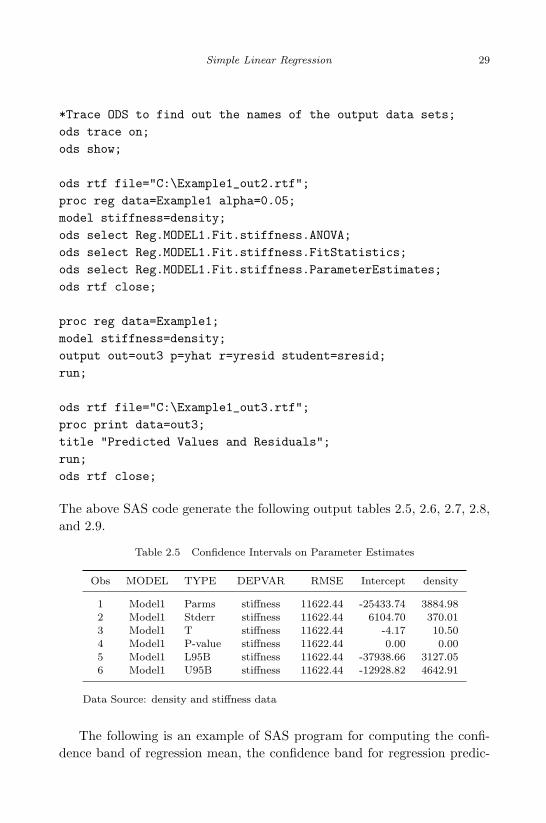
April 29, 2009 11:50 World Scientific Book - 9in x 6in Regression˙master
Simple Linear Regression 29
*Trace ODS to find out the names of the output data sets;
ods trace on;
ods show;
ods rtf file="C:\Example1_out2.rtf";
proc reg data=Example1 alpha=0.05;
model stiffness=density;
ods select Reg.MODEL1.Fit.stiffness.ANOVA;
ods select Reg.MODEL1.Fit.stiffness.FitStatistics;
ods select Reg.MODEL1.Fit.stiffness.ParameterEstimates;
ods rtf close;
proc reg data=Example1;
model stiffness=density;
output out=out3 p=yhat r=yresid student=sresid;
run;
ods rtf file="C:\Example1_out3.rtf";
proc print data=out3;
title "Predicted Values and Residuals";
run;
ods rtf close;
The above SAS code generate the following output tables 2.5, 2.6, 2.7, 2.8,and 2.9.
Table 2.5 Confidence Intervals on Parameter Estimates
Obs MODEL TYPE DEPVAR RMSE Intercept density
1 Model1 Parms stiffness 11622.44 -25433.74 3884.982 Model1 Stderr stiffness 11622.44 6104.70 370.013 Model1 T stiffness 11622.44 -4.17 10.504 Model1 P-value stiffness 11622.44 0.00 0.005 Model1 L95B stiffness 11622.44 -37938.66 3127.056 Model1 U95B stiffness 11622.44 -12928.82 4642.91
Data Source: density and stiffness data
The following is an example of SAS program for computing the confi-dence band of regression mean, the confidence band for regression predic-

April 29, 2009 11:50 World Scientific Book - 9in x 6in Regression˙master
30 Linear Regression Analysis: Theory and Computing
Table 2.6 ANOVA Table 2
Sum of MeanSource DF Squares Square F Value Pr >F
Model 1 14891739363 14891739363 110.24 <.0001Error 28 3782270481 135081089Corrected Total 29 18674009844
Data Source: density and stiffness data
Table 2.7 Regression Table
Root MSE 11622.00 R-Square 0.7975Dependent Mean 34667.00 Adj R-Sq 0.7902Coeff Var 33.53
Data Source: density and stiffness data
Table 2.8 Parameter Estimates of Simple Linear Regression
Parameter StandardVariable DF Estimate Error t Value Pr > |t|
Intercept 1 -25434.00 6104.70 -4.17 0.0003density 1 3884.98 370.01 10.50 < .0001
Data Source: density and stiffness data
tion, and probability plot (QQ-plot and PP-plot).
data Example2;
input density stiffness @@;
datalines;
9.5 14814 8.4 17502 9.8 14007 11 19443 8.3 7573
9.9 14191 8.6 9714 6.4 8076 7 5304 8.2 10728
17.4 43243 15 25319 15.2 28028 16.4 41792 16.7 49499
15.4 25312 15 26222 14.5 22148 14.8 26751 13.6 18036
25.6 96305 23.4 104170 24.4 72594 23.3 49512 19.5 32207
21.2 48218 22.8 70453 21.7 47661 19.8 38138 21.3 53045
;
across=1 cborder=red offset=(0,0)
shape=symbol(3,1) label=none value=(height=1);
symbol1 c=black value=- h=1;
symbol2 c=red;

April 29, 2009 11:50 World Scientific Book - 9in x 6in Regression˙master
Simple Linear Regression 31
Table 2.9 Table for Fitted Values and Residuals
Obs density stiffness yhat yresid
1 9.5 14814 11473.53 3340.472 8.4 17502 7200.06 10301.943 9.8 14007 12639.02 1367.984 11 19443 17300.99 2142.015 8.3 7573 6811.56 761.446 9.9 14191 13027.52 1163.487 8.6 9714 7977.05 1736.958 6.4 8076 -569.90 8645.909 7.0 5304 1761.09 3542.91
10 8.2 10728 6423.06 4304.9411 17.4 43243 42164.84 1078.1612 15.0 25319 32840.89 -7521.8913 15.2 28028 33617.89 -5589.8914 16.4 41792 38279.86 3512.1415 16.7 49499 39445.35 10053.6516 15.4 25312 34394.89 -9082.8917 15.0 26222 32840.89 -6618.8918 14.5 22148 30898.41 -8750.4119 14.8 26751 32063.90 -5312.9020 13.6 18036 27401.93 -9365.9321 25.6 96305 74021.64 22283.3622 23.4 104170 65474.69 38695.3123 24.4 72594 69359.67 3234.3324 23.3 49512 65086.19 -15574.1925 19.5 32207 50323.28 -18116.2826 21.2 48218 56927.74 -8709.7427 22.8 70453 63143.70 7309.3028 21.7 47661 58870.23 -11209.2329 19.8 38138 51488.78 -13350.7830 21.3 53045 57316.24 -4271.24
Data Source: density and stiffness data
symbol3 c=blue;
symbol4 c=blue;
proc reg data=Example2;
model density=stiffness /noprint p r;
output out=out p=pred r=resid LCL=lowpred
UCL=uppred LCLM=lowreg UCLM=upreg;
run;
ods rtf file="C:\Example2.rtf";
ods graphics on;
title "PP Plot";

April 29, 2009 11:50 World Scientific Book - 9in x 6in Regression˙master
32 Linear Regression Analysis: Theory and Computing
plot npp.*r./caxis=red ctext=blue nostat cframe=ligr;
run;
title "QQ Plot";
plot r.*nqq. /noline mse
caxis=red ctext=blue cframe=ligr;
run;
*Compute confidence band of regression mean;
plot density*stiffness/conf caxis=red ctext=blue
cframe=ligr legend=legend1;
run;
*Compute confidence band of regression prediction;
plot density*stiffness/pred caxis=red ctext=blue
cframe=ligr legend=legend1;
run;
ods graphics off;
ods rtf close;
quit;
The regression scatterplot, residual plot, 95% confidence bands for re-gression mean and prediction are presented in Fig. 2.1.
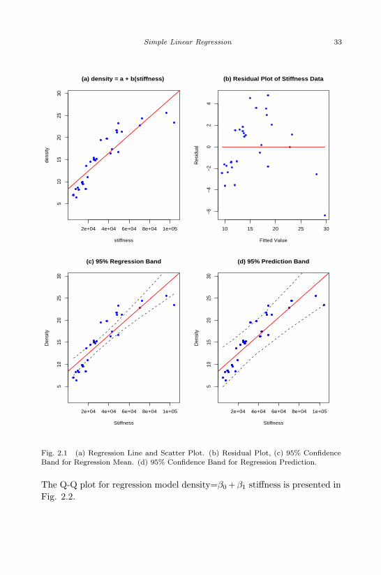
April 29, 2009 11:50 World Scientific Book - 9in x 6in Regression˙master
Simple Linear Regression 33
2e+04 4e+04 6e+04 8e+04 1e+05
510
1520
2530
(a) density = a + b(stiffness)
stiffness
dens
ity
10 15 20 25 30
−6−4
−20
24
(b) Residual Plot of Stiffness Data
Fitted Value
Res
idua
l
2e+04 4e+04 6e+04 8e+04 1e+05
510
1520
2530
(c) 95% Regression Band
Stiffness
Den
sity
2e+04 4e+04 6e+04 8e+04 1e+05
510
1520
2530
(d) 95% Prediction Band
Stiffness
Den
sity
Fig. 2.1 (a) Regression Line and Scatter Plot. (b) Residual Plot, (c) 95% ConfidenceBand for Regression Mean. (d) 95% Confidence Band for Regression Prediction.
The Q-Q plot for regression model density=β0 +β1 stiffness is presented inFig. 2.2.

May 7, 2009 10:22 World Scientific Book - 9in x 6in Regression˙master
34 Linear Regression Analysis: Theory and Computing
−2 −1 0 1 2
1015
2025
Q−Q plot for Stiffness Data
Quantile
Sam
ple
Qua
ntile
Fig. 2.2 Q-Q Plot for Regression Model density=β0 + β1 stiffness + ε.

April 29, 2009 11:50 World Scientific Book - 9in x 6in Regression˙master
Simple Linear Regression 35
Problems
1. Consider a set of data (xi, yi), i = 1, 2, · · · , n, and the following tworegression models:
yi = β0 + β1xi + ε, (i = 1, 2, · · · , n), Model A
yi = γ0 + γ1xi + γ2x2i + ε, (i = 1, 2, · · · , n), Model B
Suppose both models are fitted to the same data. Show that
SSRes, A ≥ SSRes, B
If more higher order terms are added into the above Model B, i.e.,
yi = γ0 + γ1xi + γ2x2i + γ3x
3i + · · ·+ γkxk
i + ε, (i = 1, 2, · · · , n),
show that the inequality SSRes, A ≥ SSRes, B still holds.2. Consider the zero intercept model given by
yi = β1xi + εi, (i = 1, 2, · · · , n)
where the εi’s are independent normal variables with constant varianceσ2. Show that the 100(1−α)% confidence interval on E(y|x0) is givenby
b1x0 + tα/2, n−1s
√x2
0∑ni=1 x2
i
where s =
√√√√n∑
i=1
(yi − b1xi)/(n− 1) and b1 =∑n
i=1 yixi∑ni=1 x2
i
.
3. Derive and discuss the (1−α)100% confidence interval on the slope β1
for the simple linear model with zero intercept.4. Consider the fixed zero intercept regression model
yi = β1xi + εi, (i = 1, 2, · · · , n)
The appropriate estimator of σ2 is given by
s2 =n∑
i=1
(yi − yi)2
n− 1
Show that s2 is an unbiased estimator of σ2.

April 29, 2009 11:50 World Scientific Book - 9in x 6in Regression˙master
36 Linear Regression Analysis: Theory and Computing
Table 2.10 Data for Two ParallelRegression Lines
x y
x1 y1
.
.....
xn1 yn1
xn1+1 yn1+1
..
....
xn1+n2 yn1+n2
5. Consider a situation in which the regression data set is divided into twoparts as shown in Table 2.10.The regression model is given by
yi =
β(1)0 + β1xi + εi, i = 1, 2, · · · , n1;
β(2)0 + β1xi + εi, i = n1 + 1, · · · , n1 + n2.
In other words, there are two regression lines with common slope. Usingthe centered regression model
yi =
β(1∗)0 + β1(xi − x1) + εi, i = 1, 2, · · · , n1;
β(2∗)0 + β1(xi − x2) + εi, i = n1 + 1, · · · , n1 + n2,
where x1 =∑n1
i=1 xi/n1 and x2 =∑n1+n2
i=n1+1 xi/n2. Show that the leastsquares estimate of β1 is given by
b1 =
∑n1i=1(xi − x1)yi +
∑n1+n2i=n1+1(xi − x2)yi∑n1
i=1(xi − x1)2 +∑n1+n2
i=n1+1(xi − x2)2
6. Consider two simple linear models
Y1j = α1 + β1x1j + ε1j , j = 1, 2, · · · , n1
and
Y2j = α2 + β2x2j + ε2j , j = 1, 2, · · · , n2
Assume that β1 6= β2 the above two simple linear models intersect. Letx0 be the point on the x-axis at which the two linear models intersect.Also assume that εij are independent normal variable with a varianceσ2. Show that

May 7, 2009 10:22 World Scientific Book - 9in x 6in Regression˙master
Simple Linear Regression 37
(a). x0 =α1 − α2
β1 − β2
(b). Find the maximum likelihood estimates (MLE) of x0 using theleast squares estimators α1, α2, β1, and β2.
(c). Show that the distribution of Z, where
Z = (α1 − α2) + x0(β1 − β2),
is the normal distribution with mean 0 and variance A2σ2, where
A2 =
∑x2
1j − 2x0
∑x1j + x2
0n1
n1
∑(x1j − x1)2
+
∑x2
2j − 2x0
∑x2j + x2
0n2
n2
∑(x2j − x2)2
.
(d). Show that U = Nσ2/σ2 is distributed as χ2(N), where N =n1 + n2 − 4.
(e). Show that U and Z are independent.
(f). Show that W = Z2/A2σ2 has the F distribution with degrees offreedom 1 and N .
(g). Let S21 =
∑(x1j − x1)2 and S2
2 =∑
(x2j − x2)2, show that thesolution of the following quadratic equation about x0, q(x0) =ax2
0 + 2bx0 + c = 0,[(β1 − β2)2 −
( 1S2
1
+1S2
2
)σ2Fα,1,N
]x2
0
+ 2[(α1 − α2)(β1 − β2) +
( x1
S21
+x2
S22
)σ2Fα,1,N
]x0
+[(α1 − α2)2 −
(∑ x21j
n1S21
+
∑x2
2j
n2S22
)σ2Fα,1,N
]= 0.
Show that if a ≥ 0 and b2− ac ≥ 0, then 1−α confidence intervalon x0 is
−b−√b2 − ac
a≤ x0 ≤ −b +
√b2 − ac
a.
7. Observations on the yield of a chemical reaction taken at various tem-peratures were recorded in Table 2.11:
(a). Fit a simple linear regression and estimate β0 and β1 using theleast squares method.
(b). Compute 95% confidence intervals on E(y|x) at 4 levels of temper-atures in the data. Plot the upper and lower confidence intervalsaround the regression line.

April 29, 2009 11:50 World Scientific Book - 9in x 6in Regression˙master
38 Linear Regression Analysis: Theory and Computing
Table 2.11 Chemical Reaction Data
temperature (C0) yield of chemical reaction (%)
150 77.4150 77.4150 77.4150 77.4150 77.4150 77.4150 77.4150 77.4150 77.4150 77.4150 77.4150 77.4
Data Source: Raymond H. Myers, Classical and Mod-ern Regression Analysis With Applications, P77.
(c). Plot a 95% confidence band on the regression line. Plot on thesame graph for part (b) and comment on it.
8. The study “Development of LIFETEST, a Dynamic Technique to As-sess Individual Capability to Lift Material” was conducted in VirginiaPolytechnic Institute and State University in 1982 to determine if cer-tain static arm strength measures have influence on the “dynamic lift”characteristics of individual. 25 individuals were subjected to strengthtests and then were asked to perform a weight-lifting test in whichweight was dynamically lifted overhead. The data are in Table 2.12:
(a). Find the linear regression line using the least squares method.(b). Define the joint hypothesis H0 : β0 = 0, β1 = 2.2. Test this
hypothesis problem using a 95% joint confidence region and β0
and β1 to draw your conclusion.(c). Calculate the studentized residuals for the regression model. Plot
the studentized residuals against x and comment on the plot.
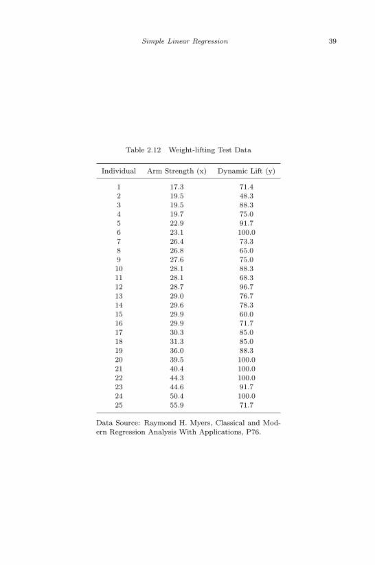
April 29, 2009 11:50 World Scientific Book - 9in x 6in Regression˙master
Simple Linear Regression 39
Table 2.12 Weight-lifting Test Data
Individual Arm Strength (x) Dynamic Lift (y)
1 17.3 71.42 19.5 48.33 19.5 88.34 19.7 75.05 22.9 91.76 23.1 100.07 26.4 73.38 26.8 65.09 27.6 75.010 28.1 88.311 28.1 68.312 28.7 96.713 29.0 76.714 29.6 78.315 29.9 60.016 29.9 71.717 30.3 85.018 31.3 85.019 36.0 88.320 39.5 100.021 40.4 100.022 44.3 100.023 44.6 91.724 50.4 100.025 55.9 71.7
Data Source: Raymond H. Myers, Classical and Mod-ern Regression Analysis With Applications, P76.

April 29, 2009 11:50 World Scientific Book - 9in x 6in Regression˙master
This page intentionally left blankThis page intentionally left blank

April 29, 2009 11:50 World Scientific Book - 9in x 6in Regression˙master
Chapter 3
Multiple Linear Regression
The general purpose of multiple linear regression is to seek for the linear re-lationship between a dependent variable and several independent variables.Multiple regression allows researchers to examine the effect of more thanone independent variables on response at the same time. For some researchquestions, regression can be used to examine how much a particular set ofindependent variables can explain sufficiently the outcome. In other cases,multiple regression is used to examine the effect of outcome while account-ing for more than one factor that could influence the outcome. In thischapter we discuss multiple linear regression. To facilitate the discussion ofthe theory of the multiple regression model we start with a brief introduc-tion of the linear space and the projection in the linear space. Then we willintroduce multiple linear model in matrix form. All subsequent discussionsof multiple regression will be based on its matrix form.
3.1 Vector Space and Projection
First we briefly discuss the vector space, subspace, projection, andquadratic form of multivariate normal variable, which are useful in thediscussions of the subsequent sections of this chapter.
3.1.1 Vector Space
A vector is a geometric object which has both magnitude and direction.A vector is frequently represented by a line segment connecting the initialpoint A with the terminal point B and denoted by
−−→AB. The magnitude
of the vector−−→AB is the length of the segment and the direction of this
vector characterizes the displacement of the point B relative to the point
41

May 7, 2009 10:22 World Scientific Book - 9in x 6in Regression˙master
42 Linear Regression Analysis: Theory and Computing
A. Vectors can be added, subtracted, multiplied by a number, and flippedaround (multiplying by number −1) so that the direction is reversed. Theseoperations obey the familiar algebraic laws: commutativity, associativity,and distributivity. The sum of two vectors with the same initial pointcan be found geometrically using the parallelogram law. Multiplicationby a positive number, commonly called a scalar in this context, amountsto changing the magnitude of vector, that is, stretching or compressing itwhile keeping its direction; multiplication by −1 preserves the magnitudeof the vector but reverses its direction. Cartesian coordinates provide asystematic way of describing vectors and operations on them.
A vector space is a set of vectors that is closed under finite vector ad-dition and scalar multiplication. The basic example is n-dimensional Eu-clidean space, where every element is represented by a list of real numbers,such as
x′= (x1, x2, · · · , xn).
Scalars are real numbers, addition is componentwise, and scalar multiplica-tion is multiplication on each term separately. Suppose V is closed undervector addition on R
n: if u, v ∈ V , then u + v ∈ V . V is also closed un-der scalar multiplication: if a ∈ R
1, v ∈ V , then av ∈ V . Then V is avector space (on R
n). We will focus our discussion only on vector spaceon n-dimensional Euclidean space. For example, for any positive integer n,the space of all n-tuples of elements of real line R
1 forms an n-dimensionalreal vector space sometimes called real coordinate space and denoted byR
n. An element in Rn can be written as
x′= (x1, x2, · · · , xn),
where each xi is an element of R1. The addition on R
n is defined by
x + y = (x1 + y1, x2 + y2, · · · , xn + yn),
and the scalar multiplication on Rn is defined by
a x = (ax1, ax2, · · · , axn).
When a = −1 the vector ax has the same length as x but with a geomet-rically reversed direction.
It was F. Hausdorff who first proved that every vector space has a basis.A basis makes it possible to express every vector of the space as a uniquetuple of the field elements, although caution must be exercised when avector space does not have a finite basis. In linear algebra, a basis is aset of vectors that, in a linear combination, can represent every vector in a

April 29, 2009 11:50 World Scientific Book - 9in x 6in Regression˙master
Multiple Linear Regression 43
given vector space, and such that no element of the set can be representedas a linear combination of the others. In other words, a basis is a linearlyindependent spanning set. The following is an example of basis of Rn:
e′1 = (1, 0, 0, · · · , 0)1×n
e′2 = (0, 1, 0, · · · , 0)1×n
e′3 = (0, 0, 1, · · · , 0)1×n
...
e′n = (0, 0, 0, · · · , 1)1×n.
Actually, the above vectors consist of the standard orthogonal basis of thevector space Rn. Any vector x
′= (x1, x2, · · · , xn) in the Rn can be a linear
combination of e1, e2, · · · ,en. In fact,
x = x1e1 + x2e2 + x3e3 + · · ·+ xnen.
This representation is unique. i.e., if there is another representation suchthat
x = x∗1e1 + x∗2e2 + x∗3e3 + · · ·+ x∗nen,
then
(x1 − x∗1)e1 + (x2 − x∗2)e2 + · · ·+ (xn − x∗n)en
= (x1 − x∗1, x2 − x∗2, · · · , x2 − x∗2) = (0, 0, · · · , 0).
Therefore, we have xi = x∗i for all i = 1, 2, · · · , n.Given a vector space V , a nonempty subset W of V that is closed
under addition and scalar multiplication is called a subspace of V . Theintersection of all subspaces containing a given set of vectors is called itsspan. If no vector can be removed without changing the span, the vectorsin this set is said to be linearly independent. A linearly independent setwhose span is V is called a basis for V . A vector span by two vectors v andw can be defined as: x : x = av + bw, for all (a, b) ∈ R2. Note that v andw may not be necessarily independent. If a vector space S is spanned by aset of independent vectors v1, v2, · · · , vp, i.e., S is the set of vectors
x : x = a1 + v1 + a2v2 + · · ·+ apvp, for all (a1, a2, · · · , ap) ∈ Rp,then the dimension of S is p. Vectors v1, v2, · · · , vp are the basis of thevector space S. The dimension of a vector space S is the largest number ofa set of independent vectors in S. If the dimension of a linear space S is p
we write Dim(S) = p.

April 29, 2009 11:50 World Scientific Book - 9in x 6in Regression˙master
44 Linear Regression Analysis: Theory and Computing
3.1.2 Linearly Independent Vectors
If there exist a finite number of distinct vectors v1, v2, · · · , vn in vectorspace V and scalars a1, a2, · · · , an, not all zero, such that
a1v1 + a2v2 + a3v3 + · · ·+ anvn = 0,
then the vectors v1, v2, · · · , vn are said to be linearly dependent. Ifv1, v2, · · · , vn are dependent then out of these n vectors there is at leastone vector that can be expressed as a linear combination of other vectors.Note that the zero on the right is the zero vector, not the number zero.If no such scalars exist, then the vectors v1, v2, · · · , vn are said to be lin-early independent. This condition can be reformulated as follows: whenevera1, a2, · · · , an are scalars such that
a1v1 + a2v2 + a3v3 + · · ·+ anvn = 0,
we have ai = 0 for i = 1, 2, · · · , n, then v1, v2, · · · , vn are linearly indepen-dent.
A basis of a vector space V is defined as a subset of vectors in V thatare linearly independent and these vectors span space V . Consequently,if (v1, v2, · · · , vn) is a list of vectors in V , then these vectors form a basisif and only if every vector x ∈ V can be uniquely expressed by a linearcombination of v1, v2, · · · , vp. i.e.,
x = a1v1 + a2v2 + · · ·+ anvn, for any x ∈ V.
The number of basis vectors in V is called the dimension of linear spaceV. Note that a vector space can have more than one basis, but the numberof vectors which form a basis of the vector space V is always fixed. i.e.,the dimension of vector space V is fixed but there will be more than onebasis. In fact, if the dimension of vector space V is n, then any n linearlyindependent vectors in V form its basis.
3.1.3 Dot Product and Projection
If x = (x1, x2, · · · , xn) and y = (y1, y2, · · · , yn) are two vectors in a vectorEuclidean space Rn. The dot product of two vectors x and y is defined as
x · y = x1y1 + x2y2 + · · ·+ xnyn.
Two vectors are said to be orthogonal if their dot product is 0. If θ is theangle between two vectors (x1, x2, · · · , xn) and (y1, y2, · · · , yn), the cosineof the angle between the two vectors is defined as
cos(θ) =x · y|x||y| =
x1y1 + x2y2 + · · ·+ xnyn√x2
1 + x22 + · · ·+ x2
n
√y21 + y2
2 + · · ·+ y2n
(3.1)

April 29, 2009 11:50 World Scientific Book - 9in x 6in Regression˙master
Multiple Linear Regression 45
Two orthogonal vectors meet at 90; i.e., they are perpendicular. Oneimportant application of the dot product is projection. The projection ofa vector y onto another vector x forms a new vector that has the samedirection as the vector x and the length |y| cos(θ), where |y| denotes thelength of vector y and θ is the angle between two vectors x and y. Wewrite this projection as Pxy. The projection vector can be expressed as
Pxy = |y| cos(θ)x
|x| = |y| x · y|x||y|
x
|x|=
x1y1 + x2y2 + · · ·+ xnyn
x21 + x2
2 + · · ·+ x2n
x = λx, (3.2)
where λ is a scalar and
λ =x1y1 + x2y2 + · · ·+ xnyn
x21 + x2
2 + · · ·+ x2n
=x · yxx
.
Thus, the projection of y onto vector x is a vector x multiplying a scalarλ where λ is the cos(θ) and θ is the angle between two vectors x and y.
If x and y are two vectors in Rn. Consider the difference vector betweenthe vector e, e = λx−y, and λ = x · y/x · x. The vector e is perpendicularto the vector x when λ = (x · y)/(x · x). To see this we simply calculatethe dot product of e and x:
e · x = (λx− y) · x = λx · x− x · y =(x · y
x · x)x · x− x · y = 0
Thus, the angle between e and x is indeed 90o, i.e., they are perpendicularto each other. In addition, since e is perpendicular to x, it is the vectorwith the shortest distance among all the vectors starting from the end of y
and ending at any point on x.If a vector space has a basis and the length of the basis vectors is a
unity then this basis is an orthonormal basis. Any basis divided by itslength forms an orthonormal basis. If S is a p-dimensional subspace of avector space V , then it is possible to project vectors in V onto S. If thesubspace S has an orthonormal basis (w1, w2, · · · , wp), for any vector y inV , the projection of y onto the subspace S is
PSy =p∑
i=1
(y · wi)wi. (3.3)
Let vector spaces S and T be the two subspaces of a vector space V andunion S ∪ T = V . If for any vector x ∈ S and any vector y ∈ T , thedot product x · y = 0, then the two vector spaces S and T are said to beorthogonal. Or we can say that T is the orthogonal space of S, denoted by
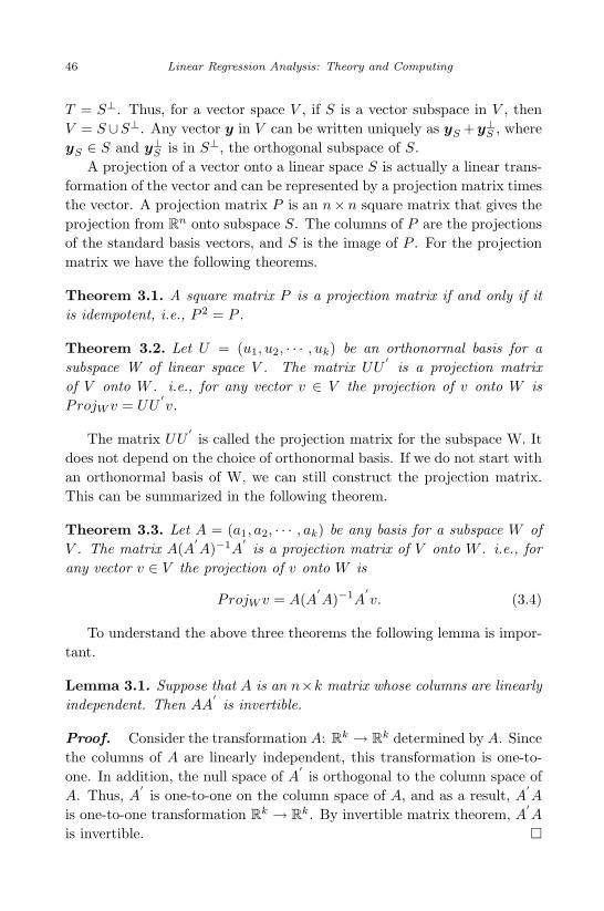
April 29, 2009 11:50 World Scientific Book - 9in x 6in Regression˙master
46 Linear Regression Analysis: Theory and Computing
T = S⊥. Thus, for a vector space V , if S is a vector subspace in V , thenV = S ∪S⊥. Any vector y in V can be written uniquely as yS +y⊥S , whereyS ∈ S and y⊥S is in S⊥, the orthogonal subspace of S.
A projection of a vector onto a linear space S is actually a linear trans-formation of the vector and can be represented by a projection matrix timesthe vector. A projection matrix P is an n×n square matrix that gives theprojection from Rn onto subspace S. The columns of P are the projectionsof the standard basis vectors, and S is the image of P . For the projectionmatrix we have the following theorems.
Theorem 3.1. A square matrix P is a projection matrix if and only if itis idempotent, i.e., P 2 = P .
Theorem 3.2. Let U = (u1, u2, · · · , uk) be an orthonormal basis for asubspace W of linear space V . The matrix UU
′is a projection matrix
of V onto W . i.e., for any vector v ∈ V the projection of v onto W isProjW v = UU
′v.
The matrix UU′is called the projection matrix for the subspace W. It
does not depend on the choice of orthonormal basis. If we do not start withan orthonormal basis of W, we can still construct the projection matrix.This can be summarized in the following theorem.
Theorem 3.3. Let A = (a1, a2, · · · , ak) be any basis for a subspace W ofV . The matrix A(A
′A)−1A
′is a projection matrix of V onto W . i.e., for
any vector v ∈ V the projection of v onto W is
ProjW v = A(A′A)−1A
′v. (3.4)
To understand the above three theorems the following lemma is impor-tant.
Lemma 3.1. Suppose that A is an n×k matrix whose columns are linearlyindependent. Then AA
′is invertible.
Proof. Consider the transformation A: Rk → Rk determined by A. Sincethe columns of A are linearly independent, this transformation is one-to-one. In addition, the null space of A
′is orthogonal to the column space of
A. Thus, A′
is one-to-one on the column space of A, and as a result, A′A
is one-to-one transformation Rk → Rk. By invertible matrix theorem, A′A
is invertible. ¤

April 29, 2009 11:50 World Scientific Book - 9in x 6in Regression˙master
Multiple Linear Regression 47
Let’s now derive the projection matrix for the column space of A. Notethat any element of the column space of A is a linear combination of thecolumns of A, i.e., x1a1 + x2a2 + · · ·+ xkak. If we write
x =
x1
x2
...xk
,
then we have
x1a1 + x2a2 + · · ·+ xkak = Ax.
Now, for any vector v ∈ Rn, we denote the projection of v onto W by xp.
ProjW v = Axp.
The projection matrix can be found by calculating xp. The projection ofvector v onto W is characterized by the fact that v−ProjW v is orthogonalto any vector w in W . Thus we have
w · (v − ProjW v) = 0
for all w in W . Since w = Ax for some x, we have
Ax · (v −Axp) = 0
for all x in Rn. Write this dot product in terms of matrices yields
(Ax)′(v −Axp) = 0
which is equivalent to
(x′A′)(v −Axp) = 0
Converting back to dot products we have
x ·A′(v −Axp) = 0
We get
A′v = A
′Axp
Since A′A is invertible we have
(A′A)−1A
′v = xp
Since Axp is the desired projection, we have
A(A′A)−1A
′v = Axp = ProjW v

April 29, 2009 11:50 World Scientific Book - 9in x 6in Regression˙master
48 Linear Regression Analysis: Theory and Computing
Therefore, we conclude that the projection matrix for W is A(A′A)−1A
′.
Projection matrix is very useful in the subsequent discussions of linearregression model Y = Xβ + ε. A squared matrix, P = X(XX
′)−1X
′, is
constructed using the design matrix. It can be easily verified that P is anidempotent matrix:
P 2 = X(XX′)−1X
′X(XX
′)−1X
′= P.
Thus, P = X(XX′)−1X
′is a projection matrix. In addition, if we define
a matrix as I −P = I −X(XX′)−1X
′. It is easy to see that I −P is also
idempotent. In fact,
(I − P )2 = I − 2P + P 2 = I − 2P + P = I − P.
Therefore, I − P = I − X(XX′)−1X
′is a projection matrix. In the
subsequent sections we will see how these projection matrices are used toobtain the best linear unbiased estimator (BLUE) for the linear regressionmodel and how they are used in regression model diagnosis.
3.2 Matrix Form of Multiple Linear Regression
In many scientific research it is often needed to determine the relation-ship between a response (or dependent) variable (y) and more than oneregressors (or independent variables) (x1, x2, · · · , xk). A general form of amultiple linear regression model is given by
y = β0 + β1x1 + β2x2 + · · ·+ βkxk + ε (3.5)
where ε is the random error. Here, regressors x1, x2, · · · , xk may containregressors and their higher order terms. In the classical setting, it is as-sumed that the error term ε has the normal distribution with a mean 0 anda constant variance σ2.
The first impression of the multiple regression may be a response plane.However, some regressors may be higher order terms of other regressors,or may even be functions of regressors as long as these functions do notcontain unknown parameters. Thus, multiple regression model can be aresponse surface of versatile shapes. Readers may already realize the dif-ference between a linear model and a nonlinear model.
Definition 3.1. A linear model is defined as a model that is linear inregression parameters, i.e., linear in βi’s.

May 7, 2009 10:22 World Scientific Book - 9in x 6in Regression˙master
Multiple Linear Regression 49
The following are examples of linear regression models in which the responsevariable y is a linear function of regression parameters:
y = β0 + β1x1 + β2x2 + β3x3 + ε,
y = β0 + β1x1 + β2x21 + β3x2 + ε,
y = β0 + β1x1 + β2x21 + β3x2 + β4x1x2 + ε,
y = β0 + β1x1 + β2ln(x1) + β2ln(x2) + ε,
y = β0 + β21(x1>5) + β21(x2>10) + β3x3 + ε.
In the last model 1(x1>5) is an indicator function taking value 1 if x1 > 5and 0 otherwise. Examples of non-linear regression model may be given by
y = β0 + β1x1 + β2xγ2 + ε,
y =1
λ + exp(β0 + β1x1 + β2x2 + · · ·+ βkxk)+ ε,
where the response variable cannot be expressed as a linear function ofregression parameters.
3.3 Quadratic Form of Random Variables
Definition 3.2. Let y′= (y1, y2, · · · , yn) be n real variables and aij be n×n
real numbers, where i, j = 1, 2, · · · , n. A quadratic form of y1, y2, · · · , yn isdefined as
f(y1, y2, · · · , yn) =n∑
i,j=1
aijyiyj .
This quadratic form can be written in the matrix form: y′Ay, where A is
an n × n matrix A = (aij)n×n. Quadratic form plays an important rolein the discussions of linear regression model. In the classical setting theparameters of a linear regression model are estimated via minimizing thesum of squared residuals:
b = (b0, b1, · · · , bk)
= arg min(β0,β1,··· ,βk)
n∑i=1
[yi − (β0 + β1x1i + β2x2i + · · ·+ βkxki)
]2.
This squared residual is actually a quadratic form. Thus, it is importantto discuss some general properties of this quadratic form that will be usedin the subsequent discussions.

April 29, 2009 11:50 World Scientific Book - 9in x 6in Regression˙master
50 Linear Regression Analysis: Theory and Computing
3.4 Idempotent Matrices
In this section we discuss properties of the idempotent matrix and its ap-plications in the linear regression. First we define the idempotent matrix.
Definition 3.3. An n× n symmetric matrix A is idempotent if A2 = A.
Let α = (α1, α2, · · · , αk) be a k-dimensional vector and A is a k × k
matrix. α′Aα is a quadratic form of α1, α2, · · · , αk. When A is an idempo-
tent matrix, the corresponding quadratic form has its particular properties.The quadratic form with idempotent matrices are used extensively in linearregression analysis. We now discuss the properties of idempotent matrix.
Theorem 3.4. Let An×n be an idempotent matrix of rank p, then the eigen-values of A are either 1 or 0.
Proof. Let λi and vi be the eigenvalue and the corresponding normalizedeigenvector of the matrix A, respectively. We then have Avi = λivi, andv′iAvi = λiv
′ivi = λi. On the other hand, since A2 = A, we can write
λi = v′iAvi = v
′iA
2vi = v′iA
′Avi = (Avi)
′Avi = (λivi)
′(λivi) = λ2
i .
Hence, we have λi(λi − 1) = 0, which yields either λi = 1 or λi = 0. Thiscompletes the proof. ¤
It is easy to know that p eigenvalues of A are 1 and n− p eigenvalues of A
are zero. Therefore, the rank of an idempotent matrix A is the sum of itsnon-zero eigenvalues.
Definition 3.4. Let A = (ai,j)n×n be an n×n matrix, trace of A is definedas the sum of the orthogonal elements. i.e.,
tr(A) = a11 + a22 + · · ·+ ann.
If A is a symmetric matrix then the sum of all squared elements of A canbe expressed by tr(A2). i.e.,
∑i,j a2
ij = tr(A2). It is easy to verify thattr(AB) = tr(BA) for any two n × n matrices A and B. The followingtheorem gives the relationship between the rank of matrix A and and traceof A when A is an idempotent matrix.
Theorem 3.5. If A is an idempotent matrix then tr(A) = rank(A) = p.
Proof. If the rank of an n × n idempotent matrix A is p then A has p
eigenvalues of 1 and n− p eigenvalues of 0. Thus, we can write rank(A) =

April 29, 2009 11:50 World Scientific Book - 9in x 6in Regression˙master
Multiple Linear Regression 51
∑ni=1 λi = p. Since A2 = A, the eigenvalues of the idempotent matrix A
is either 1 or 0. From matrix theory there is an orthogonal matrix V suchthat
V′AV =
(Ip 00 0
).
Therefore, we have
tr(V′AV ) = tr(V V
′A) = tr(A) = tr
(Ip 00 0
)= p = rank(A).
Here we use the simple fact: tr(AB) = tr(BA) for any matrices An×n andBn×n. ¤
A quadratic form of a random vector y′= (y1, y2, · · · , yn) can be written
in a matrix form y′Ay, where A is an n × n matrix. It is of interest to
find the expectation and variance of y′Ay. The following theorem gives
the expected value of y′Ay when the components of y are independent.
Theorem 3.6. Let y′
= (y1, y2, · · · , yn) be an n × 1 random vector withmean µ
′= (µ1, µ2, · · · , µn) and variance σ2 for each component. Further,
it is assumed that y1, y2, · · · , yn are independent. Let A be an n×n matrix,y′Ay is a quadratic form of random variables. The expectation of this
quadratic form is given by
E(y′Ay) = σ2tr(A) + µ
′Aµ. (3.6)
Proof. First we observe that
y′Ay = (y − µ)
′A(y − µ) + 2µ
′A(y − µ) + µ
′Aµ.
We can write
E(y′Ay) = E[(y − µ)
′A(y − µ)] + 2E[µ
′A(y − µ)] + µ
′Aµ
= E[ n∑
i,j=1
aij(yi − µi)(yj − µj)]
+ 2µ′AE(y − µ) + µ
′Aµ
=n∑
i=1
aiiE(yi − µi)2 + µ′Aµ = σ2tr(A) + µ
′Aµ.
¤

April 29, 2009 11:50 World Scientific Book - 9in x 6in Regression˙master
52 Linear Regression Analysis: Theory and Computing
We now discuss the variance of the quadratic form y′Ay.
Theorem 3.7. Let y be an n × 1 random vector with mean µ′
=(µ1, µ2, · · · , µn) and variance σ2 for each component. It is assumed thaty1, y2, · · · , yn are independent. Let A be an n × n symmetric matrix,E(yi − µi)4 = µ
(4)i , E(yi − µi)3 = µ
(3)i , and a
′= (a11, a22, · · · , ann). The
variance of the quadratic form Y′AY is given by
Var(y′Ay) = (µ(4) − 3σ2)a′a + σ4(2tr(A2) + [tr(A)]2)
+4σ2µ′A2µ + 4µ(3)a
′Aµ. (3.7)
Proof. Let Z = y − µ, A = (A1, A2, · · · , An), and b = (b1, b2, · · · , bn) =µ′(A1, A2, · · · , An) = µ
′A we can write
y′Ay = (y
′ − µ)A(y − µ) + 2µ′A(y − µ) + µ
′Aµ
= Z′AZ + 2bZ + µ
′Aµ.
Thus
Var(y′Ay) = Var(Z
′AZ) + 4V ar(bZ) + 4Cov(Z
′AZ, bZ).
We then calculate each term separately:
(Z′AZ)2 =
∑
ij
aijalmZiZjZlZm
E(Z′AZ)2 =
∑
i j l m
aijalmE(ZiZjZlZm)
Note that
E(ZiZjZlZm) =
µ(4), if i = j = k = l;σ4, if i = j, l = k or i = l, j = k, or i = k, j = l ;0, else.
We have
E(Z′AZ)2 =
∑
i j l m
aijalmE(ZiZjZlZm)
= µ(4)n∑
i=1
a2ii + σ4
( ∑
i6=k
aiiakk +∑
i 6=j
a2ij +
∑
i 6=j
aijaji
)

April 29, 2009 11:50 World Scientific Book - 9in x 6in Regression˙master
Multiple Linear Regression 53
Since A is symmetric, aij = aji, we have∑
i 6=j
a2ij +
∑
i 6=j
aijaji
= 2∑
i 6=j
a2ij = 2
∑
i,j
a2ij − 2
∑
i=j
a2ij
= 2tr(A2)− 2n∑
i=1
a2ii
= 2tr(A2)− 2a′a
and ∑
i 6=k
aiiakk =∑
i,k
aiiakk −∑
i=k
aiiakk
= [tr(A)]2 −n∑
i=1
a2ii = [tr(A)]2 − a
′a.
So we can write
E(Z′AZ)2 = (µ(4) − 3σ4)a
′a + σ4(2tr(A2) + [tr(A)]2). (3.8)
For Var(bZ) we have
Var(bZ) = bVar(Z)b′= bb
′σ2 = (µ
′A)(µ
′A)
′σ2 = µ
′A2µσ2. (3.9)
To calculate Cov(Z′AZ, bZ), note that EZ = 0, we have
Cov(Z′AZ, bZ)
= Cov(∑
i,j
aijZiZj ,∑
k
bkZk
)
=∑
i,j,k
aijbkCov(ZiZj , Zk)
=∑
i,j,k
aijbkE[(ZiZj − E(ZiZj))Zk]
=∑
i,j,k
aijbk[E(ZiZjZk)− E(ZiZj)EZk]
=∑
i,j,k
aijbk[E(ZiZjZk)] (since EZk = 0).
It is easy to know that
E(ZiZjZk) =
µ(3), if i = j = k;0, else.

April 29, 2009 11:50 World Scientific Book - 9in x 6in Regression˙master
54 Linear Regression Analysis: Theory and Computing
Thus,
Cov(Z′AZ, bZ) =
n∑
i=1
aiibiµ(3)
=n∑
i=1
aiiµ′Aiµ
(3) =n∑
i=1
aiiA′iµ µ(3) = a
′Aµ µ(3). (3.10)
Combining the results above completes the proof. ¤
3.5 Multivariate Normal Distribution
A random variable Y is said to follow the normal distribution N(µ, σ2) ifand only if the probability density function of Y is
f(y) =1√2πσ
exp− (y − µ)2
σ2
for −∞ < y < ∞. (3.11)
The cumulative distribution of Y is defined as
F (y) = P (Y ≤ y) =1√2πσ
∫ y
−∞exp
− (y − µ)2
σ2
dy. (3.12)
The moment generating function for the normal random variable Y ∼N(µ, σ) is
M(t) = E(etY ) = exp(tµ +12t2σ2). (3.13)
The multivariate normal distribution is an extension of the univariate nor-mal distribution. A random vector y
′= (y1, y2, · · · , yp) is said to follow
the multivariate normal distribution if and only if its probability densityfunction has the following form
f(y1, y2, · · · , yp) (3.14)
=1
(2π)p/2|Σ|1/2exp
− 1
2(y − µ)
′Σ−1(y − µ)
,
where Σ = (σij)p×p is the covariance matrix of y and the inverse matrixΣ−1 exists. µ
′= (µ1, µ2, · · · , µp) is the mean vector of y.
When Σ is a diagonal matrix Σ = diag(σ21 , σ2
2 , · · · , σ2p), or σij = 0 for all
i 6= j, then y1, y2, · · · , yp are not correlated since it is easy to know that the

April 29, 2009 11:50 World Scientific Book - 9in x 6in Regression˙master
Multiple Linear Regression 55
density function of y can be written as a product of p univariate normaldensity function:
1(2π)p/2|Σ|1/2
exp−1
2(y−µ)
′Σ−1(y−µ)
=
p∏
i=1
1√2πσi
exp− (yi − µi)2
σ2i
Since density function of multivariate normal vector y is a product of den-sity functions of y1, y2, · · · , yp, they are jointly independent. For multivari-ate normal variables, the uncorrelated normal random variables are jointlyindependent. We summarize this into the following theorem:
Theorem 3.8. If random vector y′= (y1, y2, · · · , yp) follows a multivari-
ate normal distribution N(µ, Σ) and the covariance matrix Σ = (σij)p×p
is a diagonal matrix diag(σ11, σ22, · · · , σpp), then y1, y2, · · · , yp are jointlyindependent.
We now introduce the central χ2 distribution. Let y1, y2, · · · , yp be p inde-pendent standard normal random variables, i.e., E(yi) = 0 and Var(yi) = 1.The special quadratic form Z =
∑pi=1 y2
i has the chi-square distributionwith p degrees of freedom and non-centrality parameter λ = 0. In addition,the random variable Z has the density function
f(z) =1
Γ(p/2)2p/2z(p−2)/2e−z/2 for 0 < z < ∞. (3.15)
The moment generating function for Z is given by
M(t) = E(etZ) = (1− 2t)−n/2 for t <12. (3.16)
Using this moment generating function it is easy to find E(Z) = p andVar(Z) = 2p. In addition, the following results are obtained through directcalculations:
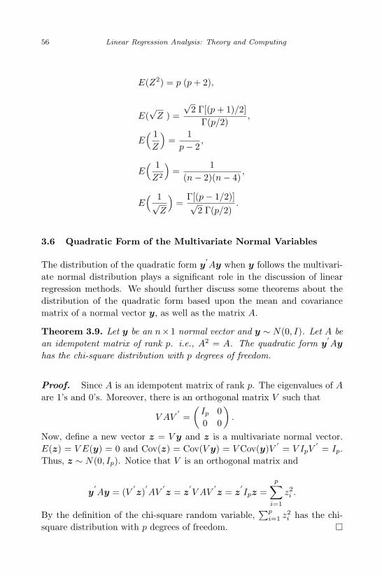
April 29, 2009 11:50 World Scientific Book - 9in x 6in Regression˙master
56 Linear Regression Analysis: Theory and Computing
E(Z2) = p (p + 2),
E(√
Z ) =√
2 Γ[(p + 1)/2]Γ(p/2)
,
E( 1
Z
)=
1p− 2
,
E( 1
Z2
)=
1(n− 2)(n− 4)
,
E( 1√
Z
)=
Γ[(p− 1/2)]√2 Γ(p/2)
.
3.6 Quadratic Form of the Multivariate Normal Variables
The distribution of the quadratic form y′Ay when y follows the multivari-
ate normal distribution plays a significant role in the discussion of linearregression methods. We should further discuss some theorems about thedistribution of the quadratic form based upon the mean and covariancematrix of a normal vector y, as well as the matrix A.
Theorem 3.9. Let y be an n× 1 normal vector and y ∼ N(0, I). Let A bean idempotent matrix of rank p. i.e., A2 = A. The quadratic form y
′Ay
has the chi-square distribution with p degrees of freedom.
Proof. Since A is an idempotent matrix of rank p. The eigenvalues of A
are 1’s and 0’s. Moreover, there is an orthogonal matrix V such that
V AV′=
(Ip 00 0
).
Now, define a new vector z = V y and z is a multivariate normal vector.E(z) = V E(y) = 0 and Cov(z) = Cov(V y) = V Cov(y)V
′= V IpV
′= Ip.
Thus, z ∼ N(0, Ip). Notice that V is an orthogonal matrix and
y′Ay = (V
′z)′AV
′z = z
′V AV
′z = z
′Ipz =
p∑
i=1
z2i .
By the definition of the chi-square random variable,∑p
i=1 z2i has the chi-
square distribution with p degrees of freedom. ¤

April 29, 2009 11:50 World Scientific Book - 9in x 6in Regression˙master
Multiple Linear Regression 57
The above theorem is for the quadratic form of a normal vector y whenEy = 0. This condition is not completely necessary. However, if thiscondition is removed, i.e., if E(y) = µ 6= 0 the quadratic form of y
′Ay
still follows the chi-square distribution but with a non-centrality parameter
λ =12µ′Aµ. We state the theorem and the proofs of the theorem should
follow the same lines as the proofs of the theorem for the case of µ = 0.
Theorem 3.10. Let y be an n × 1 normal vector and y ∼ N(µ, I). LetA be an idempotent matrix of rank p. The quadratic form y
′Ay has the
chi-square distribution with degrees of freedom p and the non-centrality pa-
rameter λ =12µ′Aµ.
We now discuss more general situation where the normal vector y followsa multivariate normal distribution with mean µ and covariance matrix Σ.
Theorem 3.11. Let y be a multivariate normal vector with mean µ and co-variance matrix Σ. If AΣ is an idempotent matrix of rank p, The quadraticform of y
′Ay follows a chi-square distribution with degrees of freedom p
and non-centrality parameter λ =12µ′Aµ.
Proof. First, for covariance matrix Σ there exists an orthogonal matrixΓ such that Σ = ΓΓ
′. Define Z = Γ−1(y − µ) and Z is a normal vector
with E(Z) = 0 and
Cov(Z) = Cov(Γ−1(y − µ)) = Γ−1Cov(y)Γ′−1 = Γ−1ΣΓ
′−1
= Γ−1(ΓΓ′)Γ
′−1 = Ip.
i.e., Z ∼ N(0, I). Moreover, since y = ΓZ + µ we have
y′Ay = [ΓZ + µ)]
′A(ΓZ + µ) = (Z
′+ Γ
′−1µ)′(Γ
′AΓ)(Z + Γ
′−1µ) = V′BV,
where V = Z′+ Γ
′−1µ ∼ N(Γ′−1µ, Ip) and B = Γ
′AΓ. We now need to
show that B is an idempotent matrix. In fact,
B2 = (Γ′AΓ)(Γ
′AΓ) = Γ
′(AΓΓ
′A)Γ
Since AΣ is idempotent we can write
AΣ = AΓΓ′= AΣAΣ = (AΓΓ
′A)ΓΓ
′= (AΓΓ
′A)Σ.
Note that Σ is non-singular we have

April 29, 2009 11:50 World Scientific Book - 9in x 6in Regression˙master
58 Linear Regression Analysis: Theory and Computing
A = AΓΓ′A.
Thus,
B2 = Γ′(AΓΓ
′A)Γ = Γ
′AΓ = B.
i.e., B is an idempotent matrix. This concludes that V′BV is a chi-square
random variable with degrees of freedom p. To find the non-centralityparameter we have
λ =12(Γ
′−1µ)′B(Γ
′−1µ)
=12µ′Γ′−1(Γ
′AΓ)Γ
′−1µ =12µ′Aµ.
This completes the proof. ¤
3.7 Least Squares Estimates of the Multiple Regression Pa-rameters
The multiple linear regression model is typically stated in the followingform
yi = β0 + β1x1i + β2x2i + · · ·+ βkxki + εi,
where yi is the dependent variable, β0, β1, β2, · · · , βk are the regressioncoefficients, and εi’s are the random errors assuming E(εi) = 0 andVar(εi) = σ2 for i = 1, 2, · · · , n. In the classical regression setting theerror term is assumed to be normally distributed with a constant vari-ance σ2. The regression coefficients are estimated using the least squaresprinciple. It should be noted that it is not necessary to assume that theregression error term follows the normal distribution in order to find theleast squares estimation of the regression coefficients. It is rather easy toshow that under the assumption of normality of the error term, the leastsquares estimation of the regression coefficients are exactly the same as themaximum likelihood estimations (MLE) of the regression coefficients.
The multiple linear model can also be expressed in the matrix format
y = Xβ + ε,

April 29, 2009 11:50 World Scientific Book - 9in x 6in Regression˙master
Multiple Linear Regression 59
where
X =
x11 x12 · · · x1k
x21 x22 · · · x2k
· · ·xn1 xn2 · · · xnk
β =
β0
β1
β2
· · ·βk−1
ε =
ε1
ε2
ε3
· · ·εn
(3.17)
The matrix form of the multiple regression model allows us to discuss andpresent many properties of the regression model more conveniently andefficiently. As we will see later the simple linear regression is a special caseof the multiple linear regression and can be expressed in a matrix format.The least squares estimation of β can be solved through the least squaresprinciple:
b = arg minβ [(y −Xβ)′(y −Xβ)],
where b′
= (b0, b1, · · · bk−1)′, a k-dimensional vector of the estimations of
the regression coefficients.
Theorem 3.12. The least squares estimation of β for the multiple linearregression model y = Xβ + ε is b = (X
′X)−1X
′y, assuming (X
′X) is
a non-singular matrix. Note that this is equivalent to assuming that thecolumn vectors of X are independent.
Proof. To obtain the least squares estimation of β we need to minimizethe residual of sum squares by solving the following equation:
∂
∂b[(y −Xb)
′(y −Xb)] = 0,
or equivalently,
∂
∂b[(y
′y − 2y
′Xb + b
′X
′Xb)] = 0.
By taking partial derivative with respect to each component of β we obtainthe following normal equation of the multiple linear regression model:
X′Xb = X
′y.
Since X′X is non-singular it follows that b = (X
′X)−1X
′y. This com-
pletes the proof. ¤
April 29, 2009 11:50 World Scientific Book - 9in x 6in Regression˙master
60 Linear Regression Analysis: Theory and Computing
We now discuss statistical properties of the least squares estimation of theregression coefficients. We first discuss the unbiasness of the least squaresestimation b.
Theorem 3.13. The estimator b = (X′X)−1X
′y is an unbiased estimator
of β. In addition,
Var(b) = (X′X)−1σ2. (3.18)
Proof. We notice that
Eb = E((X′X)−1X
′y) = (X
′X)−1X
′E(y) = (X
′X)−1X
′Xβ = β.
This completes the proof of the unbiasness of b. Now we further discusshow to calculate the variance of b. The variance of the b can be computeddirectly:
Var(b) = Var((X′X)−1X
′y)
= (X′X)−1X
′Var(b)((X
′X)−1X
′)′
= (X′X)−1X
′X(X
′X)−1σ2 = (X
′X)−1σ2. ¤
Another parameter in the classical linear regression is the variance σ2, aquantity that is unobservable. Statistical inference on regression coefficientsand regression model diagnosis highly depend on the estimation of errorvariance σ2. In order to estimate σ2, consider the residual sum of squares:
ete = (y −Xb)′(y −Xb) = y
′[I −X(X
′X)−1X
′]y = y
′Py.
This is actually a distance measure between observed y and fitted regressionvalue y. Note that it is easy to verify that P = [I − X(X
′X)−1X
′] is
idempotent. i.e.,
P 2 = [I −X(X′X)−1X
′][I −X(X
′X)−1X
′] = [I −X(X
′X)−1X
′] = P.
Therefore, the eigenvalues of P are either 1 or 0. Note that the matrixX(X
′X)−1X
′is also idempotent. Thus, we have
rank(X(X′X)−1X
′) = tr(X(X
′X)−1X
′)
= tr(X′X(X
′X)−1) = tr(Ip) = p.

April 29, 2009 11:50 World Scientific Book - 9in x 6in Regression˙master
Multiple Linear Regression 61
Since tr(A−B) = tr(A)− tr(B) we have
rank(I −X(X′X)−1X
′) = tr(I −X(X
′X)−1X
′)
= tr(In)− tr(X′X(X
′X)−1) = n− p
The residual of sum squares in the multiple linear regression is e′e whichcan be written as a quadratic form of the response vector y.
e′e = (y −Xb)′(y −Xb) = y
′(I −X(X
′X)−1X
′)y.
Using the result of the mathematical expectation of the quadratic form wehave
E(e′e) = E[y′(I −X(X
′X)−1X
′)y
]
= (Xβ)′(I −X(X
′X)−1X
′)(Xβ) + σ2(n− p)
= (Xβ)′(Xβ −X(X
′X)−1X
′Xβ) + σ2(n− p) = σ2(n− p)
We summarize the discussions above into the following theorem:
Theorem 3.14. The unbiased estimator of the variance in the multiplelinear regression is given by
s2 =e′e
n− p=
y′(I −X(X
′X)−1X
′)y
n− p=
1n− p
n∑
i=1
(yi − yi)2. (3.19)
Let P = X(X′X)−1X
′. The vector y can be partitioned into two vectors
(I − P )y = (I −X(X′X)−1X
′)y and Py = X(X
′X)−1X
′)y. Assuming
the normality of regression error term (I − P )y is independent of Py. Tosee this we simply calculate the covariance of (I − P )y and Py:
Cov((I − P )y, Py
)
= (I − P )Cov(y)P = (I − P )Pσ2
= (I −X(X′X)−1X
′)X(X
′X)−1X
′σ2
= [X(X′X)−1X
′ − (X(X′X)−1X
′)X(X
′X)−1X
′]σ2
= (X(X′X)−1X
′ −X(X′X)−1X
′)σ2 = 0
Since (I − P )y and Py are normal vectors, the zero covariance impliesthat they are independent of each other. Thus, the quadratic functions
April 29, 2009 11:50 World Scientific Book - 9in x 6in Regression˙master
62 Linear Regression Analysis: Theory and Computing
y′(I − P )y and y
′Py are independent as well. When P is idempotent,
the quadratic function of a normal vector y′Py follows the chi-square dis-
tribution with degrees of freedom p, where p = rank(P ). This propertycan be used to construct the F test statistic that is commonly used in thehypothesis testing problem for multiple linear regression.
The above calculations can be simplified if we introduce the following the-orem for the two linear transformations of a multivariate normal variabley.
Theorem 3.15. Let y ∼ N(µ, I) and A and B be two matrices. Twonormal vectors Ay and By are independent if and only if AB
′= 0.
Proof. Recall that the independence of two normal vectors is equivalentto zero covariance between them. We calculate the covariance of Ay andBy.
Cov(Ay, By) = ACov(y)B′= AB
′
Thus, the independence of two normal vectors Ay and By is equivalent toAB
′= 0. ¤
By using this theorem we can easily show that (I − P )y and Py are inde-pendent. In fact, because P is idempotent, therefore, (I−P )P = P −P 2 =P − P = 0. The result follows immediately.
3.8 Matrix Form of the Simple Linear Regression
The simple linear regression model is a special case of the multiple linearregression and can be expressed in the matrix format. In particular,
X =
1 x1
1 x2
· · ·1 xn
, β =
(β0
β1
), ε =
ε1
ε2
· · ·εn
.
The formula for calculating b in matrix format can be applied to the simplelinear regression.
X′X =
(n
∑xi∑
xi
∑x2
i
).

April 29, 2009 11:50 World Scientific Book - 9in x 6in Regression˙master
Multiple Linear Regression 63
It is not difficult to solve for (X′X)−1 analytically. In fact, the inverse
matrix of X′X is given by
(X′X)−1 =
1n
∑ni=1 x2
i − (∑n
i=1 xi)2
( ∑x2
i −∑xi
−∑xi n
)
=1
n∑n
i=1(xi − x)2
( ∑x2
i −∑xi
−∑xi n
).
The least squares estimation of the simple linear regression can be calcu-lated based on its matrix form:
b = (X′X)−1X
′y ==
1n
∑ni=1(xi − x)2
( ∑x2
i −∑xi
−∑xi n
)(∑yi∑xiyi
)
=1
n∑n
i=1(xi − x)2
(∑x2
i
∑yi −
∑xi
∑xiyi
n∑
xiyi −∑
xi
∑yi
)
=
∑x2
i
∑yi −
∑xi
∑xiyi∑n
i=1(xi − x)2
∑(xi − x)(yi − y)∑n
i=1(xi − x)2
.
Thus, we have
b0 =∑
x2i
∑yi −
∑xi
∑xiyi∑n
i=1(xi − x)2= y − b1x
and
b1 =∑
(xi − x)(yi − y)∑ni=1(xi − x)2
.
The results are exactly identical to the results derived in Chapter 2. Theunbiasness of the b and the covariance of b can be shown for the simplelinear regression using its matrix form as well. We left this to the readers.

April 29, 2009 11:50 World Scientific Book - 9in x 6in Regression˙master
64 Linear Regression Analysis: Theory and Computing
3.9 Test for Full Model and Reduced Model
Before an appropriate linear regression model is chosen it is often unknownhow many variables should be included in the regression model. A linearregression model with more variables may not always perform better thanthe regression model with less variables when both models are comparedin terms of residual of sum squares. To compare two regression models interms of the independent variables included in the models we need to test ifthe regression model with more independent variables performs statisticallybetter than the regression model with less independent variables. To thisend, we define the full regression model as:
y = X1β1 + X2β2 + ε, (3.20)
and the reduced regression model as:
y = X2β2 + ε. (3.21)
A full linear regression model is the model with more independent variablesand a reduced model is the model with a subset of the independent variablesin the full model. In other words, the reduced regression model is the modelnested in the full regression model. We would like to test the followinghypothesis
H0 : β1 = 0 versus H1 : β1 6= 0.
Under the null hypothesis H0, the error term of the regression model ε ∼N(0, σ2In). Denote X = (X1, X2), where X1 is an n× p1 matrix, X2 isan n×p2 matrix, and n is the total number of observations. A test statisticneeds to be constructed in order to compare the full regression model withthe reduced regression regression model. Consider the difference betweenthe SSE of the full model and the SSE of the reduced model:
SSEreduced = y′(I −X2(X
′2X2)−1X
′2)y
and
SSEfull = y′(I −X(X
′X)−1X
′)y,
SSEreduced − SSEfull = y′(
X(X′X)−1X
′ −X2(X′2X2)−1X
′2
)y.
The matrices X(X′X)−1X
′and X2(X
′2X2)−1X
′2 are idempotent.
In addition, it can be shown that the matrix(X(X
′X)−1X
′ −

April 29, 2009 11:50 World Scientific Book - 9in x 6in Regression˙master
Multiple Linear Regression 65
X2(X′2X2)−1X
′2
)is also idempotent and the rank of this matrix is p1
which is the dimension of β1:
Rank of(X(X
′X)−1X
′ −X2(X′2X2)−1X
′2
)
= tr(X(X
′X)−1X
′ −X2(X′2X2)−1X
′2
)
= tr(X(X
′X)−1X
′)− tr(X2(X
′2X2)−1X
′2
)
= tr(X′X(X
′X)−1)− tr(X
′2X2(X
′2X2)−1)
= (p1 + p2)− p2 = p1
The distribution of the following quadratic form is the chi-square distribu-tion with degrees of freedom p1:
y′(
X(X′X)−1X
′ −X2(X′2X2)−1X
′2
)y ∼ σ2χ2
p1.
Note that the matrix I−X(X′X)−1X
′is idempotent and its rank is n−p1.
Applying the theorem of the distribution of the quadratic form, it can beshown that total sum of residuals
s2 = y′(
I −X(X′X)−1X
′)y ∼ σ2χ2
n−p,
where p is the total number of parameters. In addition, It can be shownthat s2 is independent of SSEreduced − SSEfull. In fact, we only need toshow
[X(X
′X)−1X
′ −X2(X′2X2)−1X
′2
][I −X(X
′X)−1X
′]= 0.
It is easy to verify that
[I −X(X
′X)−1X
′][X(X
′X)−1X
′]= 0.
It remains to show
[I −X(X
′X)−1X
′][X2(X
′2X2)−1X
′2
]= 0.
It is straightforward that
[I −X(X
′X)−1X
′]X =
[I −X(X
′X)−1X
′](X1, X2) = 0.

April 29, 2009 11:50 World Scientific Book - 9in x 6in Regression˙master
66 Linear Regression Analysis: Theory and Computing
Note that X = (X1, X2) we have
[I −X(X
′X)−1X
′]X2 = 0.
Therefore,
[I −X(X
′X)−1X
′]X2
[(X
′2X2)−1X
′2
]= 0.
Thus, we can construct the following F test statistic:
F =y′(X(X
′X)−1X
′ −X2(X′2X2)−1X
′2
)y/p1
y′(I −X(X
′X)−1X
′)y/n− p
∼ Fp1,n−p. (3.22)
This test statistic can be used to test hypothesis H0 : β1 = 0 versus H1 :β1 6= 0.
3.10 Test for General Linear Hypothesis
Consider the following multiple linear regression model
y = βX + ε,
where ε ∼ N(0, σ2In). It may be of interest to test the linear function ofmodel parameters. This can be formulated into the following general linearhypothesis testing problem:
H0 : Cβ = d versus H1 : Cβ 6= d.
Here, C is a r×p matrix of rank r and r ≤ p, p is the number of parametersin the regression model, or the dimension of β. Suppose that b is the leastsquares estimation of β then we have
b ∼ N(β, σ2(X′X)−1)
and
Cb ∼ N(Cβ, σ2C(X′X)−1C
′).
Under the null hypothesis H0 : Cβ = d, we have

May 7, 2009 10:22 World Scientific Book - 9in x 6in Regression˙master
Multiple Linear Regression 67
[Cb− d ]′[C(X
′X)−1C
′]−1[Cb− d ] ∼ σ2χ2
r,
therefore, the statistic that can be used for testing H0 : Cβ = d versusH1 : Cβ = d is the F test statistic in the following form:
F =(Cb− d)
′[C(X
′X)−1C
′]−1(Cb− d)
rs2∼ Fr,n−p. (3.23)
3.11 The Least Squares Estimates of Multiple RegressionParameters Under Linear Restrictions
Sometimes, we may have more knowledge about regression parameters, orwe would like to see the effect of one or more independent variables in aregression model when the restrictions are imposed on other independentvariables. This way, the parameters in such a regression model may beuseful for answering a particular scientific problem of interest. Althoughrestrictions on regression model parameters could be non-linear we onlydeal with the estimation of parameters under general linear restrictions.Consider a linear regression model
y = βX + ε.
Suppose that it is of interest to test the general linear hypothesis: H0 :Cβ = d versus H1 : Cβ = d, where d is a known constant vector. Wewould like to explore the relationship of SSEs between the full model andthe reduced model. Here, the full model is referred to as the regressionmodel without restrictions on the parameters and the reduced model isthe model with the linear restrictions on parameters. We would like tofind the least squares estimation of β under the general linear restrictionCβ = d. Here C is a r×p matrix of rank r and r ≤ p. With a simple lineartransformation the general linear restriction Cβ = d can be rewritten asCβ∗ = 0. So, without loss of generality, we consider homogeneous linearrestriction: Cβ = 0. This will simplify the derivations. The estimator weare seeking for will minimize the least squares (y −Xβ)
′(y −Xβ) under
the linear restriction Cβ = 0. This minimization problem under the linearrestriction can be solved by using the method of the Lagrange multiplier.To this end, we construct the objective function Q(β, λ) with Lagrangemultiplier λ:

May 7, 2009 10:22 World Scientific Book - 9in x 6in Regression˙master
68 Linear Regression Analysis: Theory and Computing
Q(β, λ) = (y −Xβ)′(y −Xβ) + 2λCβ
= y′y + β
′X
′Xβ − β
′X
′y − y
′Xβ + 2λCβ
To minimize the objective function Q(β, λ), we take the partial derivativeswith respect to each component of β and with respect to λ which yieldsthe following normal equations:
X
′Xβ + Cλ = X
′y
Cβ = 0
The solutions of the above normal equation are least squares estimators ofthe regression model parameters under the linear restriction Cβ = 0. Thenormal equation can be written in the form of blocked matrix:
(X
′X C
′
C 0
)(β
λ
)=
(X
′y
0
)(3.24)
The normal equation can be easily solved if one can find the inverse matrixon the left of the above normal equation. Formula of inverse blocked matrixcan be used to solve the solution of the system. To simplify the notationswe denote X
′X = A, and the inverse matrix in blocked form is given by
(X
′X C
′
C 0
)−1
=(
A C′
C 0
)−1
=
A−1 −A−1C′(CA−1C
′)−1CA−1 A−1C(CA−1C
′)−1
(CA−1C′)−1C
′A−1 −(CA−1C
′)−1
By multiplying the blocked inverse matrix on the both sides of the abovenormal equation the least squares estimator of β under the linear restrictionis given by
b∗ = (A−1 −A−1C′(CA−1C
′)−1CA−1)X
′y. (3.25)
For the full model (the model without restriction)
SSEfull = y′(I −XA−1X
′)y.

April 29, 2009 11:50 World Scientific Book - 9in x 6in Regression˙master
Multiple Linear Regression 69
For the reduced model (the model with a linear restriction):
SSEred = y′(I −XA−1X
′+ XA−1C
′(CA−1C
′)−1CA−1X
′)y
Note that b = (X′X)−1X
′y and we have
SSEred − SSEfull = y′(XA−1C(CA−1C
′)−1CA−1X
′)y
= y′X(X
′X)−1C
′(C(X
′X)−1C
′)−1C(X
′X)−1X
′y
= (Cb)′(C(X
′X)−1C
′)−1Cb.
Under the normality assumption the above expression is a quadratic form ofthe normal variables. It can be shown that it has the chi-square distributionwith degrees of freedom as the rank of the matrix C(X
′X)−1C
′, which is
r, the number of parameters in the model. Thus, we can write
(Cb)′[C(X
′X)−1C
′]−1(Cb) ∼ σ2χ2
r. (3.26)
It can be shown that the s2 is independent of the above χ2 variable. Finally,we can construct the F test statistic:
F =(Cb)
′[C(X
′X)−1)C
′]−1(Cb)
rs2∼ Fr, n−p, (3.27)
which can be used to test the general linear hypothesis H0 : Cβ = 0 versusH1 : Cβ 6= 0.
3.12 Confidence Intervals of Mean and Prediction in Mul-tiple Regression
We now discuss the confidence intervals on regression mean and regressionprediction for multiple linear regression. For a given data point x
′0 the fit-
ted value is y|x0 = x′0b and V ar(y|x0) = x
′0Cov(b)x0 = x
′0(X
′X)−1x0σ
2.
Note that under the normality assumption on the model error termE(y|x0) = E(x0b) = x
′0β and
(y|x0)− E(y|x0)
s√
x′0(X
′X)−1x0
∼ tn−p
where n is the total number of observations and p is the number of theparameters in the regression model. Thus, the (1 − α)100% confidenceinterval for E(y|x0) is given by

May 7, 2009 10:22 World Scientific Book - 9in x 6in Regression˙master
70 Linear Regression Analysis: Theory and Computing
(y|x0)± tα/2,n−ps
√x
′0(X
′X)−1x0 (3.28)
Using the arguments similar to that in Chapter 2 the confidence intervalon regression prediction in multiple linear regression is given by:
(y|x0)± tα/2,n−ps
√1 + x
′0(X
′X)−1x0 (3.29)
3.13 Simultaneous Test for Regression Parameters
Instead of testing for regression parameters individually, we can simulta-neously test for the model parameters. We describe this simultaneous hy-pothesis test for multiple regression parameters using the vector notation:
H0 : β = β0, versus H1 : β = β0,
where β′= (β0, β1, · · · , βp−1), a p-dimensional vector of regression parame-
ters, and β′0 = (β00, β10, · · · , βp−1,0), a p-dimensional constant vector. The
above simultaneous hypothesis testing problem can be tested using the fol-lowing F test statistic which has the F distribution with degrees of freedomp and n− p under H0:
F =(b− β0)
′(X
′X)−1(b− β0)
ps2∼ Fp,n−p.
Here n is the total number of observations and p is the total number ofregression parameters. To test simultaneously the regression parameters,for a given test level α, if the observed b satisfies the following inequalityfor a chosen cut-off Fα,p,n−p,
Pr( (b− β0)
′(X
′X)−1(b− β0)
ps2≤ Fα,p,n−p
)≥ 1− α,
then H0 cannot be rejected. Otherwise, we accept H1. The F test statisticcan be used to construct the simultaneous confidence region for regressionparameters β:
β :
(b− β)′(X
′X)−1(b− β)
ps2≤ Fα,p,n−p
. (3.30)
Note that this simultaneous confidence region of the regression parametersis an ellipsoid in R
p.

April 29, 2009 11:50 World Scientific Book - 9in x 6in Regression˙master
Multiple Linear Regression 71
3.14 Bonferroni Confidence Region for Regression Param-eters
Instead of constructing an ellipsoid confidence region by a quadratic formof the regression coefficients we can set a higher confidence level for eachparameter so that the joint confidence region for all regression coefficientshas a confidence level (1−α)100%. This can be done using the Bonferroniapproach. Suppose that we have p regression coefficients and would like toconstruct a (1−α)100% joint confidence region for p regression parameters,instead of using α/2 for each regression parameter we now use a higher levelα/2p to construct the Bonferroni confidence interval for all regression pa-rameters βi, i = 1, 2, · · · , p. i.e., we choose a cut-off tα/2p, n−p and constructthe following confidence interval for each regression parameter:
bi ± tα/2p, n−p(standard error of bi).
Note that Cov(b) = (X′X)−1σ2. The standard error of bi can be estimated
by the squared root of the diagonal elements in the matrix (X′X)−1s2.
This confidence region is the p-dimensional rectangular in Rp and has ajoint confidence level of not less than 1 − α. Confidence region based onthe Bonferroni approach is conservative but the calculation is simpler.
The Bonferroni method can also be used to construct the confidence boundson regression mean. Suppose we have r data points x1, x2, · · · ,xr, andwant to construct the Bonferroni simultaneous confidence intervals on re-gression means at points x1,x2, · · · , xr. The following formula gives thesimultaneous confidence intervals for regression means at the observationsx1, x2, · · · , xr:
y(xj)± tα/2r, n−ps√
x′j(X
′X)−1xj (3.31)
The SAS code for calculating simultaneous confidence intervals on regres-sion means and regression predictions are similar to those for the sim-ple linear regression which was presented in the previous chapter for thesimple linear regression. The only difference is to set a higher confidencelevel (1−α/2r)100% for the simultaneous confidence intervals on regressionmeans at x1,x2, · · · , xr.
April 29, 2009 11:50 World Scientific Book - 9in x 6in Regression˙master
72 Linear Regression Analysis: Theory and Computing
3.15 Interaction and Confounding
We have seen that linear regression is flexible enough to incorporate certainnonlinearity in independent variables via polynomial or other transformedterms of the independent variables. It is quite useful in many applicationsthat the independent variables in the linear regression are categorical. Inthis section, we shall continue to demonstrate its great flexibility in handlingand exploring interactions. We will also show how linear regression is usedto evaluate the confounding effects among predictors.
A confounding variable (or factor) is an extraneous variable in a regressionmodel that correlates (positively or negatively) with both the dependentvariable and the independent variable. A confounding variable is associatedwith both the probable cause and the outcome. In clinical study, the com-mon ways of experiment control of the confounding factor are case-controlstudies, cohort studies, and stratified analysis. One major problem is thatconfounding variables are not always known or measurable. An interactionin a regression model often refers to as the effect of two or more indepen-dent variables in the regression model is not simply additive. Such a termreflects that the effect of one independent variable depends on the valuesof one or more other independent variables in the regression model.
The concepts of both interaction and confounding are more methodologicalthan analytic in statistical applications. A regression analysis is generallyconducted for two goals: to predict the response Y and to quantify the rela-tionship between Y and one or more predictors. These two goals are closelyrelated to each other; yet one is more emphasized than the other dependingon application contexts. For example, in spam detection, prediction accu-racy is emphasized as determining whether or not an incoming email is aspam is of primary interest. In clinical trials, on the other hand, the experi-menters are keenly interested to know if an investigational medicine is moreeffective than the control or exposure, for which the standard treatment ora placebo is commonly used, in treating some disease. The assessment oftreatment effect is often desired in analysis of many clinical trials. Bothinteraction and confounding are more pertaining to the second objective.
Consider a regression analysis involving assessment of the association be-tween the response and one (or more) predictor, which may be affectedby other extraneous predictors. The predictor(s) of major interest can beeither categorical or continuous. When it is categorical, it is often referred
April 29, 2009 11:50 World Scientific Book - 9in x 6in Regression˙master
Multiple Linear Regression 73
to as treatment in experimental designs. The difference it makes on theresponses is cited as the treatment effect. The extraneous predictors thatpotentially influence the treatment effect are termed as covariates or controlvariables. Interaction and confounding can be viewed as different mannersin which the covariates influence the treatment effect.
3.15.1 Interaction
By definition, interaction is referred to as the situation where the asso-ciation of major concern or the treatment effect varies with the levels orvalues of the covariates. Consider, for example, the treatment-by-centerinteraction in a multi-center clinical trial, a common issue involved in aclinical trial that is conducted in different medical centers. If the treat-ment effect remains the same among different medical centers, then we saythat no interaction exists between treatment and center; if the treatment isfound effective, nevertheless, more or less across different medical centers,then we say interaction exists between treatment and center and interactioninvolved is referred to as quantitative interaction; if the new treatment isfound effective than the control in some medical centers but harmful thanthe control in some other centers, then the interaction is referred to as qual-itative interaction. There is a directional change in treatment effect acrosscenters in the case of qualitative interaction while the treatment effect onlydiffers in amount, not in direction of the comparison, with quantitative in-teractions. Quantitative interactions are quite common. But if qualitativeinteraction exists, it causes much more concerns. It is thus imperative inclinical trials to detect and, if exists, fully explore and test for qualitativeinteraction. In the following discussion, we shall treat these two types ofinteraction by the same token, while referring interested readers to Gail andSimon (1985) and Yan and Su (2005) for more discussion on their importantdifferences.
In linear regression, interaction is commonly formulated by cross-product terms. Consider the regression setting of response Y and twocontinuous regressors X1 and X2. The interaction model can be stated as,ignoring the subscript i for observations,
y = β0 + β1x1 + β2x2 + β3x1x2 + ε. (3.32)
Recall that in the additive or main effect model
y = β0 + β1x1 + β2x2 + ε, (3.33)

May 7, 2009 10:22 World Scientific Book - 9in x 6in Regression˙master
74 Linear Regression Analysis: Theory and Computing
the association between Y and X1 is mainly carried by its slope β1, whichcorresponds to the amount of change in the mean response E(Y ) with oneunit increase in X1, holding X2 fixed. Here the slope β1, which does notdepend on X2, remains unchanged with different values of X2 and hencecan be interpreted as the main effect of X1. Similar interpretation holdsfor the slope β1 of X2.
x1
y
(a) main effect model
x1
y
(b) interaction model
Fig. 3.1 Response Curves of Y Versus X1 at Different Values of X2 in Models (3.33)and (3.32).
In model (3.32), we can extract the ‘slopes’ for X1 and X2 by rewriting
E(y) = (β0 + β2x2) + (β1 + β3x2) · x1
= (β0 + β1x1) + (β2 + β3x1) · x2
The slope for X1 now becomes (β1 + β3x2), which depends on what valueX2 is fixed at. For this reason, X2 is said to be an effect-modifier of X1.
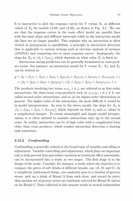
April 29, 2009 11:50 World Scientific Book - 9in x 6in Regression˙master
Multiple Linear Regression 75
It is instructive to plot the response curves for Y versus X1 at differentvalues of X2 for models (3.33) and (3.32), as shown in Fig. 3.1. We cansee that the response curves in the main effect model are parallel lineswith the same slope and different intercepts while in the interaction modelthe lines are no longer parallel. This explains why no interaction is oftenviewed as synonymous to parallelism, a principle in interaction detectionthat is applicable to various settings such as two-way analysis of variance(ANOVA) and comparing two or more response curves. Analogously, theslope for X2 is (β2 + β3x1), which depends on what value X1 is fixed at.
Interaction among predictors can be generally formulated as cross prod-uct terms. For instance, an interaction model for Y versus X1, X2, and X3
can be written as
y = β0 + β1x1 + β2x2 + β3x3 + β4x1x2 + β5x1x3 + β6x2x3 + β7x1x2x3 + ε
= (β0 + β2x2 + β3x3 + β6x2x3) + (β1 + β4x2 + β5x3 + β7x2x3) x1 + ε.
The products involving two terms xixj , i 6= j, are referred to as first-orderinteractions; the three-term cross-products such as xixjxk, i 6= j 6= k, arecalled second-order interactions; and so on for higher-order interactions ingeneral. The higher order of the interaction, the more difficult it would bein model interpretation. As seen in the above model, the slope for X1 is(β1 + β4x2 + β5x3 + β7x2x3), which depends on both x2 and x3 values ina complicated manner. To retain meaningful and simple model interpre-tation, it is often advised to consider interactions only up to the secondorder. In reality, interaction can be of high order with a complicated formother than cross products, which renders interaction detection a duntingtask sometimes.
3.15.2 Confounding
Confounding is generally related to the broad topic of variable controlling oradjustment. Variable controlling and adjustment, which plays an importantrole to help prevent bias and reduce variation in treatment effect assessment,can be incorporated into a study at two stages. The first stage is in thedesign of the study. Consider, for instance, a study where the objective is tocompare the prices of soft drinks of different brands, say, (A, B, and C). Ina completely randomized design, one randomly goes to a number of grocerystores, pick up a drink of Brand A from each store, and record its price;then another set of grocery stores are randomly selected for Brand B; and soon for Brand C. Data collected in this manner result in several independent

April 29, 2009 11:50 World Scientific Book - 9in x 6in Regression˙master
76 Linear Regression Analysis: Theory and Computing
random samples, one for each treatment or brand, and the analysis can becarried out using the one-way ANOVA technique. The potential problemwith this design, however, is that the treatment effect, as measured by thedifferences in price among the three groups, would be contaminated due toheterogeneity in other factors. Imagine what would happen if it turns outthat price data collected for Brand A are taken from stores, mostly locatedin Minnesota in winter times while data collected for Brand B are takenduring summer times from stores mostly located in Florida. In this case,we will be unable to obtain a genuine evaluation of the price difference dueto brands. A better approach in this study is to employ a randomized blockdesign with grocery stores being blocks, which can be described as follows.One randomly selects a number of grocery stores first; at each store, pickup a Brand A drink, a Brand B drink, and a Brand C drink and recordtheir prices. In this way, we are able to control for many other geographicaland longitudinal factors. By controlling, it means to make sure that theyhave the same or similar values. In general, if we know which factors arepotentially important, then we can make control for them beforehand byusing block or stratified designs.
However, very often we are pretty much blind about which factors areimportant. Sometimes, even if we have a good idea about them accordingto previous studies or literatures, we nevertheless do not have the authorityor convenience to perform the control beforehand in the design stage. Thisis the case in many observational studies. Or perhaps there are too manyof them; it is impossible to control for all. In this case, the adjustmentcan still be made in a post hoc manner at the data analysis stage. Thisis exactly what the analysis of covariance (ANCOVA) is aimed for. Theapproach is to fit models by including the important covariates.
The conception of confounding is casted into the post hoc variable ad-justment at the data analysis stage. In general, confounding occurs if in-terpretations of the treatment effect are statistically different when somecovariates are excluded or included in the model. It is usually assessedthrough a comparison between a crude estimator of the treatment effectby ignoring the extraneous variables and an estimate after adjusting forthe covariates. Consider a setting (Y vs. Z, X1, . . . , Xp), where variable Z
denotes the treatment variable of major interest and X1, . . . , Xp denote theassociated covariates. The comparison can be carried out in terms of thefollowing two models:
y = β0 + β1z + ε (3.34)

April 29, 2009 11:50 World Scientific Book - 9in x 6in Regression˙master
Multiple Linear Regression 77
and
y = β0 + β1z + α1x1 + · · ·+ αpxp + ε. (3.35)
Let β(c)1 denote the least squares estimator of β1 in model (3.34), which
gives a rudimentary assessment of the treatment effect. Let β(a)1 denote the
least squares estimator of β1 in model (3.35), which evaluates the treatmenteffect after adjusting or controlling for covariates (X1, . . . , Xp). We sayconfounding is present if these two estimates, combined with their standarderrors, are statistically different from each other. In this case, (X1, . . . , Xp)are called confounders (or confounding factors) of Z.
In the traditional assessment of confounding effects, a statistical test isnot required, perhaps because the analytical properties of (β(a)
1 − β(c)1 ) are
not easy to comprehend unless resampling techniques such as bootstrap isused. It is mainly up to field experts to decide on existence of confoundersand hence can be subjective. Another important point about confoundingis that its assessment would become irrelevant if the treatment is stronglyinteracted with covariates. Interaction should be assessed before lookingfor confounders as it no longer makes sense to purse the main or separateeffect of the treatment when it really depends on the levels or values of thecovariates.
3.16 Regression with Dummy Variables
In regression analysis, a dummy variable is one that takes the value 0 or1 to indicate the absence or presence of some categorical effect that maybe expected to shift outcome. The reason we say “dummy” because it isnot a variable that carries value of actual magnitude. For example, in aclinical trial, it is often useful to define a dummy variable D and D = 1represents treatment group and D = 0 indicates placebo group; or we canintroduce dummy variable S and define S = 1 for male group and 0 forfemale group. The mean value of a dummy variable is the proportion ofthe cases in the category coded 1. The variance of a dummy variable is∑
D2i
/n− (
∑Di
/n)2 = p− p2 = p(1− p), where p is the proportion of the
cases in the category coded 1. Example of a regression model with dummyvariable gender is:
Yi = β0 + β1Xi + β2Di + εi (3.36)

April 29, 2009 11:50 World Scientific Book - 9in x 6in Regression˙master
78 Linear Regression Analysis: Theory and Computing
where Yi is the annual salary of a lawyer, Di = 1 if the lawyer is male andDi = 0 if the lawyer is female, and Xi is years of experience. This modelassumes that there is a mean salary shift between male lawyers and femalelawyers. Thus, the mean salary is E(Yi|Di = 1) = β0 + β2 + β1Xi for amale lawyer and is E(Yi|Di = 0) = β0 +β1Xi for a female lawyer. A test ofthe hypothesis H0 : β2 = 0 is a test of the hypothesis that the wage is thesame for male lawyers and female lawyers when they have the same yearsof experience.
Several dummy variables can be used together to deal with more complexsituation where more than two categories are needed for regression analysis.For example, variable race usually refers to the concept of categorizinghumans into populations on the basis of various sets of characteristics. Avariable race can have more than two categories. Suppose that we wantedto include a race variable with three categories White/Asian/Black in aregression model. We need to create a whole new set of dummy variablesas follows
D1i = 1, if the person is whiteD1i = 0, otherwiseD2i = 1, if the person is asianD2i = 0, otherwise
Here, the ‘black’ person category is treated as the base category and thereis no need to create a dummy variable for this base category. All salarycomparisons between two races in the regression model will be relative tothe base category. In general, if there are m categories that need to be con-sidered in a regression model it is needed to create m−1 dummy variables,since the inclusion of all categories will result in perfect collinearity. Sup-pose that we would like to model the relation between the salary of a lawyerin terms of years of experience (Xi) and his/her race determined jointly bytwo dummy variables D1i, D2i, we can use the following regression modelwith the two dummy variables :
Yi = β0 + β1Xi + β2D1i + β3D2i + εi, (3.37)
where Yi is the salary of the lawyer, Xi is years of his/her working experi-ence, and D1i and D2i are dummy variables that determine the race of thelawyer. For example, based on the above regression model, the expectedsalary for a black lawyer with Xi years of working experience is

May 7, 2009 10:22 World Scientific Book - 9in x 6in Regression˙master
Multiple Linear Regression 79
E(Yi|D1i = 0, D2i = 0) = β0 + β1Xi.
The expected salary for a white lawyer with Xi years of working experienceis
E(Yi|D1i = 1, D2i = 0) = β0 + β1Xi + β2.
The expected salary for an asian lawyer with Xi years of working experienceis
E(Yi|D1i = 0, D2i = 1) = β0 + β1Xi + β3.
In each case the coefficient of the dummy variable in the regressionmodel represents the difference with the base race (the black lawyer’ssalary). Thus, the interpretation of β2 is that a white lawyer earns β2
more than a black lawyer, and the interpretation of β3 is that an asianlawyer earns β3 more than a black lawyer. The hypothesis test H0 : β2 = 0is to test whether the wage is identical for a white lawyer and a black lawyerwith same years of experience. And the hypothesis test H0 : β3 = 0 is totest that whether the wage is identical for an asian lawyer and a blacklawyer with same years of experience.
Furthermore, if we would like to consider race effect and gender effect to-gether, the following model with multiple dummy variables can be used:
Yi = β0 + β1Xi + β2D1i + β3D2i + β4Di + εi (3.38)
According to model (3.38), for example, the expected salary for a femaleblack lawyer with Xi years of experience is
E(Yi|D1i = 0, D2i = 0, Di = 0) = β0 + β1Xi.
For a black male lawyer with Xi years of experience, the expected salary is
E(Yi|D1i = 0, D2i = 0, Di = 1) = β0 + β1Xi + β4.
For a white male lawyer with Xi years of experience, the expected salary is

May 7, 2009 10:22 World Scientific Book - 9in x 6in Regression˙master
80 Linear Regression Analysis: Theory and Computing
E(Yi|D1i = 1, D2i = 0, Di = 1) = β0 + β1Xi + β2 + β4.
The hypothesis test H0 : β4 = 0 is to test if the wage is the same formale lawyer and female lawyer with the same years of experience. Thehypothesis test H0 : β2 = β4 = 0 is to test if the wage is the same for malewhite lawyer and black lawyer with the same years of experience and if thegender has no impact on the salary.
If we have k categories then k − 1 dummy variables are needed. This isbecause in the classical regression it is required that none of exploratoryvariable should be a linear combination of remaining exploratory modelvariables to avoid collinearity. For example, we can use the dummy variableD and code D = 1 for male, if we also use another dummy variable S =0 to indicate female, then there is a linear relation between D and S:D = 1 − S. Therefore, information become redundant. Thus, one dummyvariable should be sufficient to represent information on gender. In general,k− 1 dummy variables are sufficient to represent k categories. Note that ifDi’s, i = 1, 2, · · · , k− 1, are k− 1 dummy variables then Di = 1 representsa category out of the total k categories, and all Di = 0 represents the basecategory out of the total k categories. Thus, k − 1 dummy variables aresufficient to represent k distinct categories.
If a regression model involves a nominal variable and the nominal vari-able has more than two levels, it is needed to create multiple dummy vari-ables to replace the original nominal variable. For example, imagine thatyou wanted to predict depression level of a student according to status offreshman, sophomore, junior, or senior. Obviously, it has more than twolevels. What you need to do is to recode “year in school” into a set ofdummy variables, each of which has two levels. The first step in this pro-cess is to decide the number of dummy variables. This is simply k − 1,where k is the number of levels of the original nominal variable. In thisinstance, 3 dummy variables are needed to represent 4 categories of studentstatus.
In order to create these variables, we are going to take 3 levels of “yearin school”, and create a variable corresponding to each level, which willhave the value of yes or no (i.e., 1 or 0). In this example, we create threevariables sophomore, junior, and senior. Each instance of “year in school”would then be recoded into a value for sophomore, junior, and senior. Ifa person is a junior, then variables sophomore and senior would be equal

April 29, 2009 11:50 World Scientific Book - 9in x 6in Regression˙master
Multiple Linear Regression 81
to 0, and variable junior would be equal to 1. A student with all variablessophomore, junior, and senior being all 0 is a freshman.
The decision as to which level is not coded is often arbitrary. The levelwhich is not coded is the category to which all other categories will becompared. As such, often the biggest group will be the not-coded category.In a clinical trial often the placebo group or control group can be chosenas the not-coded group. In our example, freshman was not coded so thatwe could determine if being a sophomore, junior, or senior predicts a differ-ent depression level than being a freshman. Consequently, if the variable“junior” is significant in our regression, with a positive coefficient β, thiswould mean that juniors are significantly more depressive than freshmen.Alternatively, we could have decided to not code “senior”, then the coeffi-cients for freshman, sophomore and junior in the regression model would beinterpreted as how much more depressive if being a freshman, sophomore,or junior predicts a different depressive level than being a senior.
For the purpose of illustration, the simple regression model with one dummyvariable is shown in Fig. 3.2. In the figure, (a) represents regression modelwith only dummy variable and without regressor. The two groups areparallel. (b) represents the model with dummy variable and regressor x,but two groups are still parallel, (c) represents the model with dummyvariable and regressor x. The two groups are not parallel but withoutcrossover. (d) represents the model with dummy variable and regressor x.The two groups are not parallel and with crossover. In situations (c) and(d) we say that there is interaction which means that the response of onegroup is not always better/higher than the response of the other group bythe same magnitude. Situation (c) is quantitative interaction and (d) isqualitative interaction or crossover interaction.
3.17 Collinearity in Multiple Linear Regression
3.17.1 Collinearity
What is the collinearity in multiple linear regression? The collinearity refersto the situation in which two or more independent variables in a multiplelinear regression model are highly correlated. Let the regression model bey = X+ε with the design matrix X = (1, x1, x2, · · · ,xk). The collinearityoccurs if the independent variable xi is highly linearly correlated to anotherone or more independent variables xj1,xj2, · · · , xjk. In other words, xi

April 29, 2009 11:50 World Scientific Book - 9in x 6in Regression˙master
82 Linear Regression Analysis: Theory and Computing
2 4 6 8
02
46
8(a). Paralell Groups
x
resp
onse
y=2
y=4
2 4 6 80
24
68
10
(b). Paralell Groups
x
resp
onse
y=0.2+0.5x
y=2.2+0.5x
2 4 6 8
02
46
810
(c). Unparalell Groups without Crossover
x
resp
onse
y=1+0.5 x
y=2.6
7+0.6
3 x
2 4 6 8
02
46
810
(d). Unparalell Groups with Crossover
x
resp
onse
Fig. 3.2 Regression on Dummy Variables
can be almost linearly expressed by one or more other column vectors inX. In this situation, the matrix X
′X is ill-conditioned or near singular.
Although it is not completely singular, its eigenvalues may be close to zeroand the eigenvalues of the inverse matrix (X
′X)−1 tend to be very large
which may cause instability of the least squares estimates of the regressionparameters. If there is a perfect collinearity among column vectors of X
then the matrix X′X is not invertible. Therefore, it is problematic to

April 29, 2009 11:50 World Scientific Book - 9in x 6in Regression˙master
Multiple Linear Regression 83
solve for the unique least squares estimators of the regression coefficientsfrom the normal equation. When the column vectors of the design matrixX is highly correlated, then the matrix XtX becomes ill-conditioned andthe least squares estimator become less reliable even though we can finda unique solution of the normal equation. To see this let’s look at thefollowing example of two simple data sets (Tables 3.1 and 3.2).
Table 3.1 Two Independent Vectors
x1 10 10 10 10 15 15 15 15x2 10 10 15 15 10 10 15 15
Table 3.2 Two Highly Correlated Vectors
x1 10.0 11.0 11.9 12.7 13.3 14.2 14.7 15.0x2 10.0 11.4 12.2 12.5 13.2 13.9 14.4 15.0
The correlation matrix of the vectors in the first example data is a 2 × 2identity matrix
X′X =
(1 00 1
).
Thus, its inverse matrix is also a 2 × 2 identity matrix. The correlationmatrix of the two vectors in the second example data set is
X′X =
(1.00000 0.992150.99215 1.00000
)
and its inverse matrix is given by
(X′X)−1 =
(63.94 −63.44
−64.44 63.94
).
Note that for linear regression, Var(b) = (X′X)−1σ2. For the vectors in
the first example data set we have
Var(b1)σ2
=Var(b2)
σ2= 1.

April 29, 2009 11:50 World Scientific Book - 9in x 6in Regression˙master
84 Linear Regression Analysis: Theory and Computing
For the vectors in the second example data set we have
Var(b1)σ2
=Var(b2)
σ2= 63.94
The variances of the regression coefficients are inflated in the example ofthe second data set. This is because the collinearity of the two vectors inthe second data set. The above example is the two extreme cases of therelationship between the two vectors. One is the case where two vectorsare orthogonal to each other and the other is the case where two vectorsare highly correlated.
Let us further examine the expected Euclidean distance between the leastsquares estimate b and the true parameter β, E(b − β)
′(b − β) when
collinearity exists among the column vectors of X. First, it is easy toknow that E[(b− β)
′(b− β)] = E(b
′b)− β
′β. We then calculate E(b
′b).
E(b′b)
= E[(X′X)−1X
′y′(X
′X)−1X
′y]
= E[y′X(X
′X)−1(X
′X)−1X
′y]
= (Xβ)′X(X
′X)−1(X
′X)−1X
′Xβ + σ2tr[X(X
′X)−1(X
′X)−1X
′]
= β′X
′X(X
′X)−1(X
′X)−1X
′Xβ + σ2tr[X
′X(X
′X)−1(X
′X)−1]
= β′β + σ2tr[(X
′X)−1]
Thus, we have
E[(b− β)′(b− β)] = σ2tr[(X
′X)−1].
Note that E[(b − β)′(b − β)] is the average Euclidean distance measure
between the estimate b and the true parameter β. Assuming that (X′X)
has k distinct eigenvalues λ1, λ2, · · · , λk, and the corresponding normalizedeigenvectors V = (v1, v2, · · · , vk), we can write
V′(X
′X)V = diag(λ1, λ2, · · · , λk).
Moreover,
tr[V′(X
′X)V ] = tr[V V
′(X
′X)] = tr(X
′X) =
k∑
i=1
λi.

April 29, 2009 11:50 World Scientific Book - 9in x 6in Regression˙master
Multiple Linear Regression 85
Since the eigenvalues of (X′X)−1 are
1λ1
,1λ2
, · · · ,1λk
we have
E(b′b) = β
′β + σ2
k∑
i=1
1λi
,
or it can be written as
E( k∑
i=1
b2i
)=
k∑
i=1
β2i + σ2
k∑
i=1
1λi
. (3.39)
Now it is easy to see that if one of λ is very small, say, λi = 0.0001, thenroughly,
∑ki=1 b2
i may over-estimate∑k
i=1 β2i by 1000σ2 times. The above
discussions indicate that if some columns in X are highly correlated withother columns in X then the covariance matrix (XX
′)−1σ2 will have one
or more large eigenvalues so that the mean Euclidean distance of E[(b −β)
′(b − β)] will be inflated. Consequently, this makes the estimation of
the regression parameter β less reliable. Thus, the collinearity in columnvectors of X will have negative impact on the least squares estimates ofregression parameters and this need to be examined carefully when doingregression modeling.
How to deal with the collinearity in the regression modeling? One easyway to combat collinearity in multiple regression is to centralize the data.Centralizing the data is to subtract mean of the predictor observations fromeach observation. If we are not able to produce reliable parameter estimatesfrom the original data set due to collinearity and it is very difficult to judgewhether one or more independent variables can be deleted, one possibleand quick remedy to combat collinearity in X is to fit the centralized datato the same regression model. This would possibly reduce the degree ofcollinearity and produce better estimates of regression parameters.
3.17.2 Variance Inflation
Collinearity can be checked by simply computing the correlation matrix ofthe original data X. As we have discussed, the variance inflation of theleast squares estimator in multiple linear regression is caused by collinearityof the column vectors in X. When collinearity exists, the eigenvalues ofthe covariance matrix (X
′X)−1σ2 become extremely large, which causes
severe fluctuation in the estimates of regression parameters and makes these

April 29, 2009 11:50 World Scientific Book - 9in x 6in Regression˙master
86 Linear Regression Analysis: Theory and Computing
estimates less reliable. Variance inflation factor is the measure that can beused to quantify collinearity. The ith variance inflation factor is the scaledversion of the multiple correlation coefficient between the ith independentvariable and the rest of the independent variables. Specifically, the varianceinflation factor for the ith regression coefficient is
VIFi =1
1−R2i
, (3.40)
where R2i is the coefficient of multiple determination of regression produced
by regressing the variable xi against the other independent variables xj , j 6=i. Measure of variance inflation is also given as the reciprocal of the aboveformula. In this case, they are referred to as tolerances.
If Ri equals zero (i.e., no correlation between xi and the remaining in-dependent variables), then VIFi equals 1. This is the minimum value ofvariance inflation factor. For the multiple regression model it is recom-mended looking at the largest VIF value. A VIF value greater than 10 maybe an indication of potential collinearity problems. The SAS procedureREG provides information on variance inflation factor and tolerance foreach regression coefficient. The following example illustrates how to obtainthis information using SAS procedure REG.
Example 3.1. SAS code for detection of collinearity and calculation thevariance inflation factor.
Data example;
input x1 x2 x3 x4 x5 y;
datalines;
15.57 2463 472.92 18.0 4.45 566.52
44.02 2048 1339.75 9.5 6.92 696.82
20.42 3940 620.25 12.8 4.28 1033.15
18.74 6505 568.33 36.7 3.90 1603.62
49.20 5723 1497.60 35.7 5.50 1611.37
44.92 11520 1365.83 24.0 4.6 1613.27
55.48 5779 1687.00 43.3 5.62 1854.17
59.28 5969 1639.92 46.7 5.15 2160.55
94.39 8461 2872.33 78.7 6.18 2305.58
128.02 20106 3655.08 180.5 6.15 3503.93
96.00 13313 2912.00 60.9 5.88 3571.89
131.42 10771 3921.00 103.7 4.88 3741.40
127.21 15543 3865.67 126.8 5.50 4026.52

April 29, 2009 11:50 World Scientific Book - 9in x 6in Regression˙master
Multiple Linear Regression 87
252.90 36194 7684.10 157.7 7.00 10343.81
409.20 34703 12446.33 169.4 10.78 11732.17
463.70 39204 14098.40 331.4 7.05 15414.94
510.22 86533 15524.00 371.6 6.35 18854.45
;
run;
proc reg data=example corr alpha=0.05;
model y=x1 x2 x3 x4 x5/tol vif collin;
run;
*Fit the regression model after deleting variable X1;
proc reg data=example corr alpha=0.05; ;
model y=x2 x3 x4 x5/tol vif collin;
run;
The keyword TOL requests tolerance values for the estimates, VIF givesthe variance inflation factors with the parameter estimates, and COLLINrequests a detailed analysis of collinearity among regressors. Variance infla-tion (VIF) is the reciprocal of tolerance (TOL). The above SAS proceduresproduce the following Table 3.3. The table shows that variables x1 and x3
are highly correlated. Due to this high correlation the variance inflation forboth the variables x1 and x3 are rather significant and it can be found inTable 3.4.
We then delete variable x1 and recalculate the correlation matrix. Itcan be seen that the variance inflations for all independent variables becomemuch smaller after deleting x1. The results of the correlation matrix andvariance inflation are presented in Tables 3.5 and 3.6.
The least squares estimates in the regression model including the in-dependent variables x2, x3, x4 and x5 behave much better than the modelincluding all independent variables. The collinearity is eliminated by delet-ing one independent variable x1 in this example.
3.18 Linear Model in Centered Form
The linear model can be rewritten in terms of centered x’s as
yi = β0 + β1xi1 + β2xi2 + · · ·+ βkxik + εi
= α + β1(xi1 − x1) + β2(xi2 − x2) + · · ·+ βk(xik − xk) + εi (3.41)

April 29, 2009 11:50 World Scientific Book - 9in x 6in Regression˙master
88 Linear Regression Analysis: Theory and Computing
Table 3.3 Correlation Matrix for Variables x1, x2, · · · , x5
Variable x1 x2 x3 x4 x5 y
x1 1.0000 0.9074 0.9999 0.9357 0.6712 0.9856x2 0.9074 1.0000 0.9071 0.9105 0.4466 0.9452x3 0.9999 0.9071 1.0000 0.9332 0.6711 0.9860x4 0.9357 0.9105 0.9332 1.0000 0.4629 0.9404x5 0.6712 0.4466 0.6711 0.4629 1.0000 0.5786y 0.9856 0.9452 0.9860 0.9404 0.5786 1.0000
Table 3.4 Parameter Estimates and Variance Inflation
Variable Parameter STD t value P > |t| Tolerance Inflation
Intercept 1962.95 1071.36 1.83 0.094 0x1 -15.85 97.66 -0.16 0.874 0.0001042 9597.57x2 0.06 0.02 2.63 0.023 0.12594 7.94x3 1.59 3.09 0.51 0.617 0.000112 8933.09x4 -4.23 7.18 -0.59 0.569 0.04293 23.29x5 -394.31 209.64 -1.88 0.087 0.23365 4.28
Table 3.5 Correlation Matrix after Deleting Variable x1
Variable x2 x3 x4 x5 y
x2 1.0000 0.9071 0.9105 0.4466 0.9452x3 0.9071 1.0000 0.9332 0.6711 0.9860x4 0.9105 0.9332 1.0000 0.4629 0.9404x5 0.4466 0.6711 0.4629 1.0000 0.5786y 0.9452 0.9860 0.9404 0.5786 1.0000
Table 3.6 Variance Inflation after Deleting x1
variable parameter std t value P > |t| tolerance inflation
intercept 2032.19 942.075 2.16 0.0520 0x2 0.056 0.020 2.75 0.0175 0.126 7.926x3 1.088 0.153 7.10 < .0001 0.042 23.927x4 -5.00 5.081 -0.98 0.3441 0.079 12.706x5 -410.083 178.078 -2.30 0.0400 0.298 3.361
for i = 1, . . . , n, where
α = β0 + β1x1 + · · ·+ βkxk
or
β0 = α− (β1x1 + · · ·+ βkxk) = α− x′β1; (3.42)
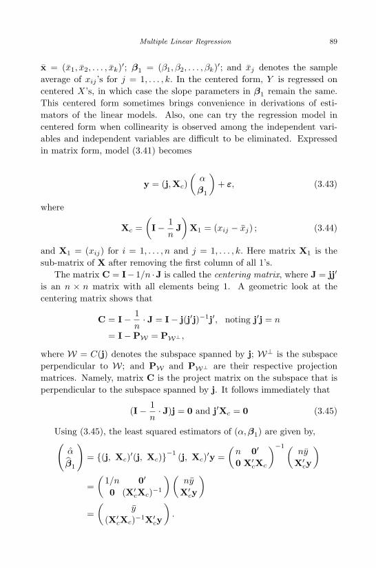
April 29, 2009 11:50 World Scientific Book - 9in x 6in Regression˙master
Multiple Linear Regression 89
x = (x1, x2, . . . , xk)′; β1 = (β1, β2, . . . , βk)′; and xj denotes the sampleaverage of xij ’s for j = 1, . . . , k. In the centered form, Y is regressed oncentered X’s, in which case the slope parameters in β1 remain the same.This centered form sometimes brings convenience in derivations of esti-mators of the linear models. Also, one can try the regression model incentered form when collinearity is observed among the independent vari-ables and independent variables are difficult to be eliminated. Expressedin matrix form, model (3.41) becomes
y = (j,Xc)(
α
β1
)+ ε, (3.43)
where
Xc =(I− 1
nJ)
X1 = (xij − xj) ; (3.44)
and X1 = (xij) for i = 1, . . . , n and j = 1, . . . , k. Here matrix X1 is thesub-matrix of X after removing the first column of all 1’s.
The matrix C = I− 1/n ·J is called the centering matrix, where J = jj′
is an n × n matrix with all elements being 1. A geometric look at thecentering matrix shows that
C = I− 1n· J = I− j(j′j)−1j′, noting j′j = n
= I−PW = PW⊥ ,
where W = C(j) denotes the subspace spanned by j; W⊥ is the subspaceperpendicular to W; and PW and PW⊥ are their respective projectionmatrices. Namely, matrix C is the project matrix on the subspace that isperpendicular to the subspace spanned by j. It follows immediately that
(I− 1n· J)j = 0 and j′Xc = 0 (3.45)
Using (3.45), the least squared estimators of (α, β1) are given by,(
α
β1
)= (j, Xc)′(j, Xc)−1 (j, Xc)′y =
(n 0′
0 X′cXc
)−1 (ny
X′cy
)
=(
1/n 0′
0 (X′cXc)−1
)(ny
X′cy
)
=(
y
(X′cXc)−1X′
cy
).

April 29, 2009 11:50 World Scientific Book - 9in x 6in Regression˙master
90 Linear Regression Analysis: Theory and Computing
Thus, β1 is the same as in the ordinary least squares estimator β1 and
β0 = y − x′β1 (3.46)
in view of (3.42) and uniqueness of LSE.Using the centered form, many interesting properties of the least squares
estimation can be easily obtained. First, the LS fitted regression planesatisfies
y − α = y − y = (x− x)′β1
and hence must pass through the center of the data (x, y).Denote Vc = C(Xc). Since W = C(j) ⊥ Vc using (3.45),
V = C(X) = W ⊕Vc.
The vector fitted values is
y = PVy = PWy + PVc y = yj + Xc(X′cXc)−1X′
cy = yj + Xcβ1 (3.47)
and the residual vector is
e = (I−PW −PVc)y = (PW⊥ −PVc)y. (3.48)
Consider the sum of squared error (SSE), which becomes
SSE = ‖ y − y ‖2= e′e
= y′(PW⊥ −PVc)y = y′PW⊥y − y′PVc y
=n∑
i=1
(yi − y)2 − β′1X
′cy = SST− β
′1X
′cy. (3.49)
Namely, the sum of squares regression (SSR) is SSR = β′1X
′cy.
The leverage hi = x′i(X′X)−1xi can also be reexpressed for better inter-
pretation using the centered form. Letting x1i = (xi1, x2i, . . . , xik)′,
hi = (1, x′1i − x′) (j, Xc)′(j, Xc)−1(
1x1i − x
)
= (1, x′1i − x′)(
1/n 0′
0 (X′cXc)−1
)(1
x1i − x
)
=1n
+ (x1i − x)′(XcXc)−1(x1i − x). (3.50)

April 29, 2009 11:50 World Scientific Book - 9in x 6in Regression˙master
Multiple Linear Regression 91
Note that
XcXc = (n− 1)Sxx, (3.51)
where
Sxx =
s21 s12 · · · s1k
s21 s22 · · · s2k
......
...sk1 sk2 · · · s2
k
with
s2
j =∑n
i=1(xij − xj)2
sjj′ =∑n
i=1(xij − xj)(xij′ − xj′)
is the sample variance-covariance matrix for x vectors. Therefore, hi in(3.50) is
hi =1n
+(x1i − x)′S−1
xx (x1i − x)n− 1
. (3.52)
Clearly, the term (x1i − x)′S−1xx (x1i − x) gives the Mahalanobis distance
between x1i and the center of the data x, which renders hi an importantdiagnostic measure for assessing how outlying an observation is in terms ofits predictor values.
Furthermore, both β0 and β1 can be expressed in terms of the samplevariances and covariances. Let syx denote the covariance vector between Y
and Xj ’s. Namely,
syx = (sy1, sy2, . . . , syk)′, (3.53)
where
syj =∑n
i=1(xij − xj) · (yi − y)n− 1
=∑n
i=1(xij − xj) · yi
n− 1.
It can be easily seen that
(n− 1) · syx = X′y. (3.54)
Using equations (3.51) and (3.54), we have
β1 =(
X′cXc
n− 1
)−1 X′cy
n− 1= S−1
xx syx (3.55)
and
β0 = y − β′1x = y − s′yxS
−1xx x. (3.56)
The above forms are now analogous to those formulas for β1 and β0 insimple linear regression.

April 29, 2009 11:50 World Scientific Book - 9in x 6in Regression˙master
92 Linear Regression Analysis: Theory and Computing
Besides, the coefficient of determination R2 can also be expressed interms of Sxx and syx as below
R2 =SSRSST
=β′1X
′cXcβ1∑n
i=1(yi − y)2
=s′yxS
−1xx (n− 1)SxxS−1
xx syx∑ni=1(yi − y)2
=s′yx S−1
xx syx
s2y
. (3.57)
3.19 Numerical Computation of LSE via QR Decomposi-tion
According to earlier derivation, the least squares estimator β is obtainedby solving the normal equations
X′Xβ = X′y. (3.58)
Nevertheless, the approach is not very computationally attractive becauseit can be difficult to form matrices in (3.58) to a great numerical accuracy.Instead, computation of LSE, as well as many other related quantities, iscarried out through QR decomposition of the design matrix X. The basicidea of this approach utilizes a successive orthogonalization process on thepredictors to form an orthogonal basis for the linear space V = C(X).
3.19.1 Orthogonalization
To motivate, we first consider the simple regression (Y versus X) withdesign matrix X = (j,x). The LSE of β1 is given by
β1 =∑n
i=1(xi − x) · (yi − y)∑ni=1(xi − x)2
=∑n
i=1(xi − x) · yi∑ni=1(xi − x)2
=〈x− xj,y〉
〈x− xj,x− xj〉 ,
where 〈x,y〉 = xty denotes the inner product between x and y. The aboveestimate β1 can be obtained in two steps, either applying a simple linearregression without intercept. In step 1, regress x on j without interceptand obtain the residual e = x− xj; and in step 2, regress y on the residuale without intercept to produce β1.
Note that regressing u on v without intercept by fitting model
ui = γvi + εi

April 29, 2009 11:50 World Scientific Book - 9in x 6in Regression˙master
Multiple Linear Regression 93
gives
γ =〈u,v〉〈v,v〉 and residual vector e = u− γv, (3.59)
which is exactly the step in linear algebra taken to orthogonalize one vectoru with respect to another vector v. The key point is to ensure residual vectore to be orthogonal to v, i.e., e ⊥ v or 〈e,v〉 = 0.
Orthogonality often provides great convenience and efficiency in de-signed experiments. It is easy to show, for example, that if the k predictorsx1,x2, . . . ,xk in a multiple linear regression model are orthogonal to eachother, then the LSE of the j-th slope equals
βj =〈xj ,y〉〈xj ,xj〉 ,
which is the same as the slope estimator obtained in a simple linear regres-sion model that regresses y on xj . This implies that orthogonal predictorshave no confounding effect on each other at all.
In the two-step approach, the subspace C(j,x) spanned by (j,x) is thesame as the subspace spanned by the orthogonal basis (j, e). This ideacan be generalized to multiple linear regression, which leads to the algo-rithm outlined below. This is the well-known Gram-Schmidt procedure forconstructing an orthogonal basis from an arbitrary basis. Given a designmatrix X = (x0 = j,x1, . . . ,xk) with columns xj , the result of the algo-rithm is an orthogonal basis (e0,e1, . . . , ek) for the column subspace of X,
V = C(X).
Algorithm 9.1: Gram-Schmidt Algorithm for Successive Orthogonalization.
• Set e0 = j;
• Compute γ01 = 〈x1, e0〉/〈e0, e0〉 and e1 = x1 − γ01 e0;
• Compute γ02 = 〈x2, e0〉/〈e0, e0〉 and γ12 = 〈x2, e1〉/〈e1, e1〉 and ob-tain e2 = x2 − (γ02 e0 + γ12 e1).
...
• Continue the process up to xk, which involves computing(γ0k, γ1k, . . . , γ(k−1)k) with γjk = 〈xk, ej〉/〈ej , ej〉 for j = 0, 1, . . . , (k−1) and then obtaining ek = xk− (γ0k e0 + γ1k e1 + · · ·+ γ(k−1)k ek−1).
Note that ej ⊥ ej′ for j 6= j′. It is interesting and insightful to take afew observations, as listed below. First, the slope estimate obtained by

April 29, 2009 11:50 World Scientific Book - 9in x 6in Regression˙master
94 Linear Regression Analysis: Theory and Computing
regressing y on ek without intercept is the same as the LS slope estimatefor xk in multiple linear model of y versus (x0,x1, . . . ,xk). That is,
βk =〈y, ek〉〈ek, ek〉 =
〈y,ek〉‖ ek ‖2 . (3.60)
This can be verified by using the fact that ej ’s form an orthogonal basis forthe column space of X and xk is only involved in ek = xk −
∑k−1j=0 γjkej ,
with coefficient 1.Secondly, since (e0, e1, . . . ek−1) spans the same subspace as
(x0,x1, . . . ,xk−1) does, the residual vector ek is identical to the residualvector obtained by regressing xk versus (x0,x1, . . . ,xk−1). This is the resultthat motivates the partial regression plots, in which the residuals obtainedfrom regressing y on (x0,x1, . . . ,xk−1) are plotted versus ek.
Thirdly, the same results clearly hold for any one of the predictorsif one rearranges it to the last position. The general conclusion is thatthe j-th slope βj can be obtained by fitting a simple linear regressionof y on the residuals obtained from regressing xj on other predictors(x0,x1, . . . ,xj−1,xj+1, . . . ,xk). Thus, βj can be interpreted as the addi-tional contribution of xj on y after xj has been adjusted for other predic-tors. Furthermore, from (3.60) the variance of βk is
Var(βk) =σ2
‖ ek ‖2 . (3.61)
In other words, ek, which represents how much of xp is unexplained byother predictors, plays an important role in estimating βk.
Fourthly, if xp is highly correlation with some of the other predictors, asituation to which multicolinearity is referred, then the residual vector ek
will be close to zero in length |e|. From (3.60), the estimate βk would bevery unstable. From (3.61), the precision of the estimate would be poor aswell. The effect due to multicolinearity is clearly true for all predictors inthe correlated predictors.
3.19.2 QR Decomposition and LSE
The Gram-Schmidt algorithm can be represented in matrix form. It can beeasily verified that
γjl =〈xl, ej〉〈ej , ej〉 =
1 if j = l
0 if j < l(3.62)

April 29, 2009 11:50 World Scientific Book - 9in x 6in Regression˙master
Multiple Linear Regression 95
for j, l = 0, 1, . . . , k. Denoting
Γ = (γjl) =
1 γ01 γ02 · · · γ0(k−1) γ0k
0 1 γ12 · · · γ1(k−1) γ1k
......
......
...0 0 0 · · · 1 γ(k−1)k
0 0 0 · · · 0 1
and E = (e0, e1, . . . , ek),
we have
X = EΓ = (ED−1)(DΓ) = QR, (3.63)
where D = diag(djj) with djj =‖ ej−1 ‖ for j = 1, . . . , (k + 1). The formgiven in (3.63) is the so-called QR decomposition of X. The matrix
Q = ED−1 (3.64)
is an orthogonal matrix of dimension n × (k + 1) satisfying Q′Q = I andthe matrix
R = DΓ (3.65)
is a (k + 1)× (k + 1) upper triangular matrix.Using the decomposition in (3.63), the normal equations becomes
XtXβ = Xty
=⇒ R′QtQRβ = R′Q′y
=⇒ Rβ = Qy, (3.66)
which are easy to solve since R is upper triangular. This leads to the LSE
β = R−1Q′y. (3.67)
Its variance-covariance matrix can be expressed as
Cov(β) = σ2 · (XtX)−1 = σ2 · (RtR)−1 = σ2 ·R−1(Rt)−1. (3.68)
To compute, R−1 is needed. Since R is upper triangular, R−1 = W canbe easily obtained with back-substitution in the system of linear equations
RW = I. (3.69)
Various other desired quantities in linear regression including the F
test statistic for linear hypotheses can also be computed using the QRdecomposition. For example, the predicted vector is
y = Xβ = QQty,
the residual vector is
e = y − y = (I−QQt)y
and the sum of squared errors (SSE) is
SSE = ete = yt(I−QQt)y =‖ y ‖2 − ‖ Qty ‖2 .

April 29, 2009 11:50 World Scientific Book - 9in x 6in Regression˙master
96 Linear Regression Analysis: Theory and Computing
3.20 Analysis of Regression Residual
3.20.1 Purpose of the Residual Analysis
Definition 3.5. The residual of the linear regression model y = Xβ + ε
is defined as the difference between observed response variable y and thefitted value y, i.e., e = y − y.
The regression error term ε is unobservable and the residual is observ-able. Residual is an important measurement of how close the calculatedresponse from the fitted regression model to the observed response. Thepurposes of the residual analysis are to detect model mis-specification andto verify model assumptions. Residuals can be used to estimate the er-ror term in regression model, and the empirical distribution of residualscan be utilized to check the normality assumption of the error term (QQplot), equal variance assumption, model over-fitting, model under-fitting,and outlier detection. Overall, residual analysis is useful for assessing aregression model.
Simple statistical properties of the regression residual can be discussed.The ith residual of the linear regression model can be written as
ei = yi − yi = yi − xib = yi − xi(X′X)−1X
′y.
Regression residual can be expressed in a vector form
e = y −X(X′X)−1X
′y = (I −X(X
′X)−1X
′)y = (I −H)y, (3.70)
where H = X(X′X)−1X
′is called the HAT matrix. Note that I −H is
symmetric and idempotent, i.e., I −H = (I −H)2. The covariance matrixof the residual e is given by:
Cov(e) = (I −H)Var(y)(I −H)′= (I −H)σ2.
Denote the hat matrix H = (hij) we have
Var(ei) = (1− hii)σ2
and
Cov(ei, ej) = −hijσ2.
The HAT matrix contains useful information for detecting outliers andidentifying influential observations.
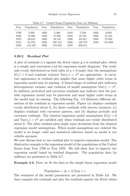
April 29, 2009 11:50 World Scientific Book - 9in x 6in Regression˙master
Multiple Linear Regression 97
Table 3.7 United States Population Data (in Millions)
Year Population Year Population Year Population Year Population
1790 3.929 1800 5.308 1810 7.239 1820 9.6381830 12.866 1840 17.069 1850 23.191 1860 31.4431870 39.818 1880 50.155 1890 62.947 1900 75.9941910 91.972 1920 105.710 1930 122.775 1940 131.6691950 151.325 1960 179.323 1970 203.211
3.20.2 Residual Plot
A plot of residuals ei’s against the fitted values yi’s is residual plot, whichis a simple and convenient tool for regression model diagnosis. The resid-uals evenly distributed on both sides of y = 0 imply that the assumptionsE(ε) = 0 and constant variance Var(εi) = σ2 are appropriate. A curva-ture appearance in residual plot implies that some higher order terms inregression model may be missing. A funnel shape of residual plot indicatesheterogeneous variance and violation of model assumption Var(ε) = σ2.In addition, periodical and curvature residuals may indicate that the pos-sible regression model may be piecewise and some higher order terms inthe model may be missing. The following Fig. 3.3 illustrate different sit-uations of the residuals in regression model. Figure (a) displays residualsevenly distributed about 0, (b) shows residuals with uneven variances, (c)displays residuals with curvature pattern, and (d) displays periodic andcurvature residuals. The classical regression model assumptions E(ε) = 0and Var(εi) = σ2 are satisfied only when residuals are evenly distributedabout 0. The other residual plots imply some deviations from the classicalregression model assumptions. When model assumptions are violated themodel is no longer valid and statistical inference based on model is notreliable anymore.We now discuss how to use residual plot to improve regression model. Theillustrative example is the regression model of the populations of the UnitedStates from Year 1790 to Year 1970. We will show how to improve theregression model based on residual diagnosis. The population data (inmillions) are presented in Table 3.7.
Example 3.2. First, we fit the data to the simple linear regression model
Population = β0 + β1Year + ε.
The estimates of the model parameters are presented in Table 3.8. Wethen compute the residuals and plot the residuals against the fitted values
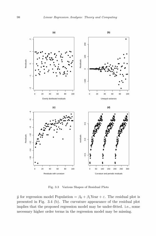
April 29, 2009 11:50 World Scientific Book - 9in x 6in Regression˙master
98 Linear Regression Analysis: Theory and Computing
0 20 40 60 80 100
−2
−1
01
2(a)
Evenly distributed residuals
Re
sid
ua
ls
0 20 40 60 80 100
−1
00
01
00
20
0
(b)
Unequal variances
Re
sid
ua
ls
0 20 40 60 80 100
−1
6−
14
−1
2−
10
−8
−6
−4
(c)
Residuals with curvature
Re
sid
ua
ls
0 50 100 150 200 250 300
−0
.50
.00
.5
(d)
Curvature and periodic residuals
resi
du
als
Fig. 3.3 Various Shapes of Residual Plots
y for regression model Population = β0 + β1Year + ε. The residual plot ispresented in Fig. 3.4 (b). The curvature appearance of the residual plotimplies that the proposed regression model may be under-fitted. i.e., somenecessary higher order terms in the regression model may be missing.
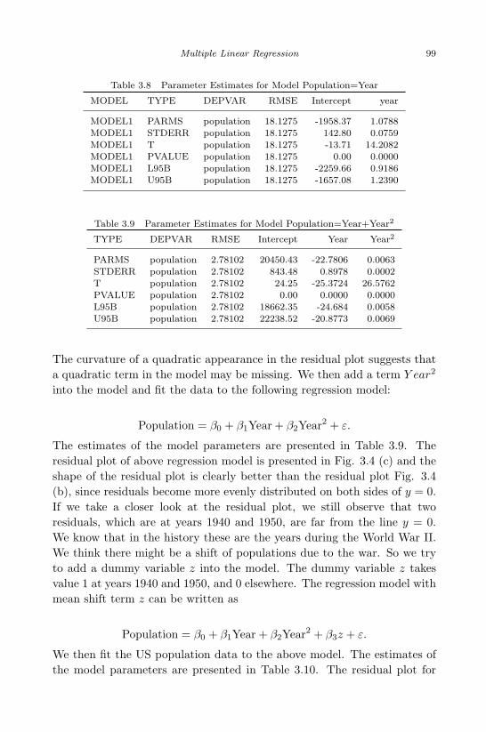
April 29, 2009 11:50 World Scientific Book - 9in x 6in Regression˙master
Multiple Linear Regression 99
Table 3.8 Parameter Estimates for Model Population=Year
MODEL TYPE DEPVAR RMSE Intercept year
MODEL1 PARMS population 18.1275 -1958.37 1.0788MODEL1 STDERR population 18.1275 142.80 0.0759MODEL1 T population 18.1275 -13.71 14.2082MODEL1 PVALUE population 18.1275 0.00 0.0000MODEL1 L95B population 18.1275 -2259.66 0.9186MODEL1 U95B population 18.1275 -1657.08 1.2390
Table 3.9 Parameter Estimates for Model Population=Year+Year2
TYPE DEPVAR RMSE Intercept Year Year2
PARMS population 2.78102 20450.43 -22.7806 0.0063STDERR population 2.78102 843.48 0.8978 0.0002T population 2.78102 24.25 -25.3724 26.5762PVALUE population 2.78102 0.00 0.0000 0.0000L95B population 2.78102 18662.35 -24.684 0.0058U95B population 2.78102 22238.52 -20.8773 0.0069
The curvature of a quadratic appearance in the residual plot suggests thata quadratic term in the model may be missing. We then add a term Y ear2
into the model and fit the data to the following regression model:
Population = β0 + β1Year + β2Year2 + ε.
The estimates of the model parameters are presented in Table 3.9. Theresidual plot of above regression model is presented in Fig. 3.4 (c) and theshape of the residual plot is clearly better than the residual plot Fig. 3.4(b), since residuals become more evenly distributed on both sides of y = 0.If we take a closer look at the residual plot, we still observe that tworesiduals, which are at years 1940 and 1950, are far from the line y = 0.We know that in the history these are the years during the World War II.We think there might be a shift of populations due to the war. So we tryto add a dummy variable z into the model. The dummy variable z takesvalue 1 at years 1940 and 1950, and 0 elsewhere. The regression model withmean shift term z can be written as
Population = β0 + β1Year + β2Year2 + β3z + ε.
We then fit the US population data to the above model. The estimates ofthe model parameters are presented in Table 3.10. The residual plot for
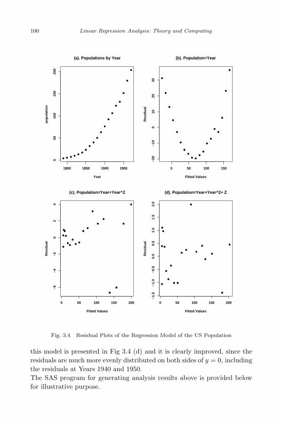
April 29, 2009 11:50 World Scientific Book - 9in x 6in Regression˙master
100 Linear Regression Analysis: Theory and Computing
1800 1850 1900 1950
050
100
150
200
(a). Populations by Year
Year
popu
latio
n
0 50 100 150
−20
−10
010
2030
(b). Population=Year
Fitted Values
Res
idua
l
0 50 100 150 200
−6
−4
−2
02
4
(c). Population=Year+Year^2
Fitted Values
Res
idua
l
0 50 100 150 200
−1.
5−
1.0
−0.
50.
00.
51.
01.
52.
0
(d). Population=Year+Year^2+ Z
Fitted Values
Res
idua
l
Fig. 3.4 Residual Plots of the Regression Model of the US Population
this model is presented in Fig 3.4 (d) and it is clearly improved, since theresiduals are much more evenly distributed on both sides of y = 0, includingthe residuals at Years 1940 and 1950.The SAS program for generating analysis results above is provided belowfor illustrative purpose.

April 29, 2009 11:50 World Scientific Book - 9in x 6in Regression˙master
Multiple Linear Regression 101
Table 3.10 Parameter Estimates for Regression Model Population=β0 +β1 Year+β2 Year2+z
TYPE DEPVAR RMSE Intercept Year Year2 z
PARMS population 0.93741 20982.75 -23.3664 0.0065 -8.7415STDERR population 0.93741 288.25 0.3071 0.0001 0.7793
T population 0.93741 72.79 -76.0838 79.5883 -11.2170PVALUE population 0.93741 0.00 0.0000 0.0000 0.0000
L95B population 0.93741 20368.37 -24.0210 0.0063 -10.4026U95B population 0.93741 21597.14 -22.7118 0.0067 -7.0805
data pop; set pop;
yyear=year*year;
if year in (1940, 1950) then z=1;
else z=0;
run;
proc reg data=pop outest=out1 tableout;
model population=year;
output out=out2
p=yhat r=yresid student=sresid;
run;
proc reg data=pop outest=out3 tableout;
model population=year yyear;
output out=out4
p=yhat r=yresid student=sresid;
run;
proc reg data=pop outest=out5 tableout;
model population=year yyear z;
output out=out6
p=yhat r=yresid student=sresid;
run;
proc gplot data=out2; symbol v=dot h=1;
plot yresid*yhat/caxis=red ctext=blue vref=0;
title "population=year";
proc gplot data=out4; symbol v=dot h=1;

April 29, 2009 11:50 World Scientific Book - 9in x 6in Regression˙master
102 Linear Regression Analysis: Theory and Computing
plot yresid*yhat/caxis=red ctext=blue vref=0;
title "population=year+year*year";
proc gplot data=out6; symbol v=dot h=1;
plot yresid*yhat/caxis=red ctext=blue vref=0;
title "population=year+year*year +Z";
run;
The above regression analysis of the US population over years can be per-formed using the free software R. One advantage of software R over SAS isthat R generates regression diagnosis graphs relatively easily. We presentthe following R code that perform the regression analysis of the US pop-ulation over years and generate all regression diagnosis plots in postscriptformat for different regression models.
year<-c(1790,1800,1810,1820,1830,1840,1850,1860,1870,1880,
1890,1900,1910,1920,1930,1940,1950,1960,1970)
pop<-c(3.929,5.308,7.239,9.638,12.866,17.069,23.191,31.443,
39.818,50.155, 62.947,75.994,91.972,105.710,122.775,
131.669,151.325,179.323,203.211)
postscript("C:\\uspop.eps",horizontal=FALSE, onefile= FALSE,
print.it=FALSE)
par(mfrow=c(2, 2))
plot(pop~year, pch=20, font=2, font.lab=2,
ylab="population",xlab="Year",
main="populations by Year")
fit<-lm(pop~year)
fitted<-fit$fitted
resid<-fit$residual
plot(fitted, resid, pch=20, cex=1.5, font=2, font.lab=2,
ylab="Residual", xlab="Fitted Values",
main="Population=Year")
yyear<-year*year
fit1<-lm(pop ~ year + yyear)
fitted1<-fit1$fitted
resid1<-fit1$residual

April 29, 2009 11:50 World Scientific Book - 9in x 6in Regression˙master
Multiple Linear Regression 103
plot(fitted1, resid1, pch=20, cex=1.5, font=2, font.lab=2,
ylab="Residual", xlab="Fitted Values",
main="population=Year+Year^2")
z<-ifelse((year==1940)|(year==1950), 1, 0)
fit2<-lm(pop ~ year + yyear +z)
fitted2<-fit2$fitted
resid2<-fit2$residual
plot(fitted2, resid2, pch=20, cex=1.5, font=2, font.lab=2,
ylab="Residual", xlab="Fitted Values",
main="population=Year+Year^2+ Z")
dev.off()
3.20.3 Studentized Residuals
Without normalization the usual residual ei = yi − yi is subject to thescale of the response yi. It is inconvenient when several regression modelsare discussed together. We then consider the normalized residual. SinceVar(ei) = (1− hii)σ2 the normalized regression residual can be defined as
ri =ei
s√
1− hii
. (3.71)
This normalized residual is called the studentized residual. Note that σ isunknown and it can be estimated by s. The studentized residual is scale-free and can be used for checking model assumption. Also it can be used formodel diagnosis. If several regression models need to be compared the scale-free studentized residuals is a better measurement for model comparison.
3.20.4 PRESS Residual
The PRESS residual is the leave-one-out residual. To obtain the PRESSresidual we fit the regression model without using the ith observation andcalculate the fitted value from that model
yi,−i = xib−i,
where b−i is the least squares estimate of regression parameters withoutusing the ith observation. yi,−i is the fitted value calculated from the re-gression model without using the ith observation. The ith PRESS residualis defined as
ei,−i = yi − yi,−i = yi − xib−i. (3.72)

April 29, 2009 11:50 World Scientific Book - 9in x 6in Regression˙master
104 Linear Regression Analysis: Theory and Computing
The PRESS residual is the measurement of influential effect of the ith obser-vation on the regression model. If the ith observation has a small influenceon the regression model then yi should be fairly close to yi,−i, therefore,the PRESS residual ei,−i should be close to the usual residual ei. In orderto discuss the PRESS residual and establish the relationship between usualthe residual ei and the PRESS residual ei,−i we first introduce the followingthe theorem (see Rao, 1973).
Theorem 3.16. Let A be a nonsingular square p × p matrix and z be ap-dimensional column vector. The matrix (A− zz
′)−1 is given by
(A− zz′)−1 = A−1 +
A−1zz′A−1
1− z′A−1z. (3.73)
The proof of the theorem is to directly show that A − zz′
multiply thematrix on the right side of the above formula yields an identity matrix. Thistheorem will be used later to establish the relationship between the PRESSresidual and the ordinary residual. For regression model y = Xβ +ε, writeX as (1,x2, x2, · · · , xp), where xi is an n-dimensional vector. It is easy toverify that
X′X =
n 1′x1 1
′x2 · · · 1
′xp
1′x1 x
′1x1 x
′1x2 · · · x
′1xp
1′x2 x
′1x1 x
′2x2 · · · x
′2xp
· · ·
1′xp x
′2xp x
′3x2 · · · x
′pxp
=
n∑
j x1j
∑j x2i · · · ∑
j xpj
∑j x1j
∑j x2
1j
∑j x1jx2j · · · ∑
j x1jxpj
∑j x2j
∑j x2jx2j
∑j x2
2j · · · ∑j x2jxpj
· · ·∑
j xpj
∑j xpjxpj
∑j xpjx2j · · · ∑
j x2pj
.
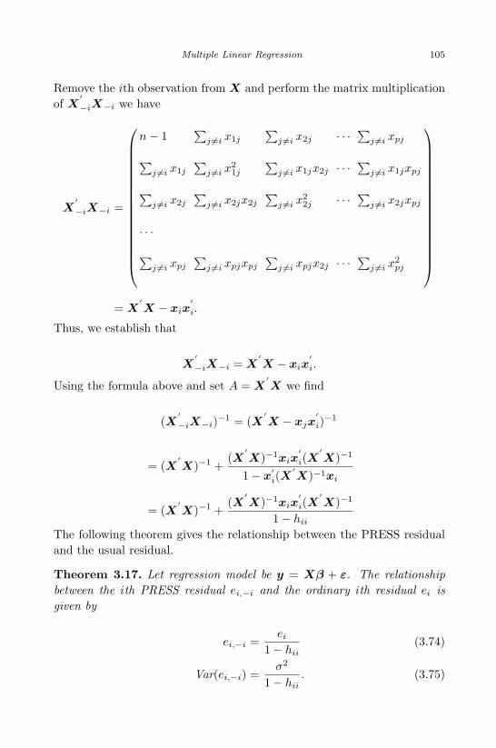
April 29, 2009 11:50 World Scientific Book - 9in x 6in Regression˙master
Multiple Linear Regression 105
Remove the ith observation from X and perform the matrix multiplicationof X
′−iX−i we have
X′−iX−i =
n− 1∑
j 6=i x1j
∑j 6=i x2j · · · ∑
j 6=i xpj
∑j 6=i x1j
∑j 6=i x2
1j
∑j 6=i x1jx2j · · · ∑
j 6=i x1jxpj
∑j 6=i x2j
∑j 6=i x2jx2j
∑j 6=i x2
2j · · · ∑j 6=i x2jxpj
· · ·∑
j 6=i xpj
∑j 6=i xpjxpj
∑j 6=i xpjx2j · · · ∑
j 6=i x2pj
= X′X − xix
′i.
Thus, we establish that
X′−iX−i = X
′X − xix
′i.
Using the formula above and set A = X′X we find
(X′−iX−i)−1 = (X
′X − xjx
′i)−1
= (X′X)−1 +
(X′X)−1xix
′i(X
′X)−1
1− x′i(X
′X)−1xi
= (X′X)−1 +
(X′X)−1xix
′i(X
′X)−1
1− hii
The following theorem gives the relationship between the PRESS residualand the usual residual.
Theorem 3.17. Let regression model be y = Xβ + ε. The relationshipbetween the ith PRESS residual ei,−i and the ordinary ith residual ei isgiven by
ei,−i =ei
1− hii(3.74)
Var(ei,−i) =σ2
1− hii. (3.75)

April 29, 2009 11:50 World Scientific Book - 9in x 6in Regression˙master
106 Linear Regression Analysis: Theory and Computing
Proof. For the regression model without using the ith observation theresidual is
ei,−i = yi − x′ib−i = yi − x
′i(X
′−iX−i)−1X
′−iy−i
= yi − x′i
[(X
′X)−1 +
(X′X)−1xix
′i(X
′X)−1
1− hii
]X
′−iy−i
=(1− hii)yi − (1− hii)x
′i(X
′X)−1X
′−iy−i − hiix
′i(X
′X)−1X
′−iy−i
1− hii
=(1− hii)yi − x
′i(X
′X)−1X
′−iy−i
1− hii
Note that X′−iy−i + xiyi = X
′y we have
ei,−i =(1− hii)yi − x
′i(X
′X)−1(X
′y − xiyi)
1− hii
=(1− hii)yi − x
′i(X
′X)−1X
′y + x
′i(X
′X)−1xiyi
1− hii
=(1− hii)yi − yi + hiiyi
1− hii=
yi − yi
1− hii=
ei
1− hii
For variance of PRESS residual Var(ei,−i) we have
Var(ei,−i) = Var(ei)1
(1− hii)2= [σ2(1− hii)]
1(1− hii)2
=σ2
1− hii ¤
The ith standardized PRESS residual is
ei,−i
σi,−i=
ei
σ√
1− hii
. (3.76)
3.20.5 Identify Outlier Using PRESS Residual
The standardized PRESS residual can be used to detect outliers since it isrelated to the ith observation and is scale free. If the ith PRESS residualis large enough then the ith observation may be considered as a potentialoutlier. In addition to looking at the magnitude of the ith PRESS residual,according to the relationship between the PRESS residual ei,−i and theregular residual ei, the ith observation may be a potential outlier if theleverage hii is close to 1.

April 29, 2009 11:50 World Scientific Book - 9in x 6in Regression˙master
Multiple Linear Regression 107
We now discuss how to deal with outlier in regression model. First, what isan outlier? An outlier is an observation at which the fitted value is not closeenough to the observed response. i.e., there is breakdown in the model atthe ith observation such that the location of the response is shifted. In thissituation, the ith data point could be a potential outlier. To mathematicallyformulate this mean shift or model breakdown, we can write E(εi) = ∆ 6= 0.i.e., there is a non-zero mean shift in error term at the ith observation. Ifwe believe that the choice and model assumptions are appropriate, it issuspectable that the ith observation might be an outlier in terms of theshift of the response from the model at that observation.
Another aspect of an outlier is that at the ith data point the Var(ε) exceedsthe error variance at other data points. i.e., there might be an inflation invariance at the ith observation. If the equal variance assumption is appro-priate we may consider the ith observation as an outlier if the variance isinflated at the ith observation. So, outlier could be examined by checkingboth the mean response shift and the variance inflation at the ith datapoint. If equal variance assumption is no longer appropriate in the regres-sion model we can use the generalized least squares estimate where theequal variance assumption is not required. The generalized least squaresestimate will be discussed later.
A convenient test statistic used to detect outlier in regression model is theith PRESS residual
ei,−i = yi − yi,−i.
If there is a mean shift at the ith data point, then we have
E(yi − yi,−i) = E(e)i,−i = ∆i > 0.
Similarly, if there is a variance inflation at the ith data point we would liketo use the standardized PRESS residual
ei,−i
σi,−i=
ei
σ√
1− hii
to detect a possible outlier. Since σ is unknown, we can replace σ by itsestimate s to calculate the standardized PRESS residual. Note that in thepresence of a mean shift outlier s is not an ideal estimate of true standarddeviation of σ. If we consider the situation where there is a mean shiftoutlier, the sample standard deviation s is biased upward, and is not anideal estimate of standard error σ. One way to cope with it is to leave the
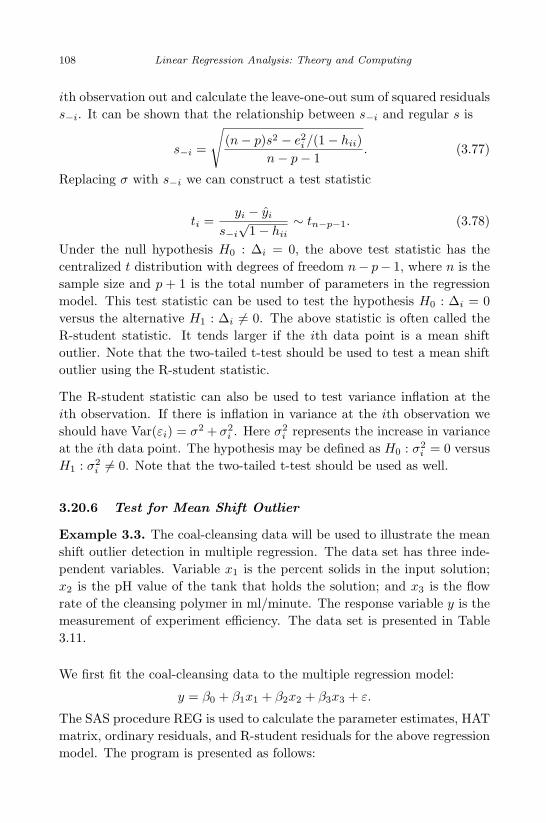
April 29, 2009 11:50 World Scientific Book - 9in x 6in Regression˙master
108 Linear Regression Analysis: Theory and Computing
ith observation out and calculate the leave-one-out sum of squared residualss−i. It can be shown that the relationship between s−i and regular s is
s−i =
√(n− p)s2 − e2
i /(1− hii)n− p− 1
. (3.77)
Replacing σ with s−i we can construct a test statistic
ti =yi − yi
s−i
√1− hii
∼ tn−p−1. (3.78)
Under the null hypothesis H0 : ∆i = 0, the above test statistic has thecentralized t distribution with degrees of freedom n− p− 1, where n is thesample size and p + 1 is the total number of parameters in the regressionmodel. This test statistic can be used to test the hypothesis H0 : ∆i = 0versus the alternative H1 : ∆i 6= 0. The above statistic is often called theR-student statistic. It tends larger if the ith data point is a mean shiftoutlier. Note that the two-tailed t-test should be used to test a mean shiftoutlier using the R-student statistic.
The R-student statistic can also be used to test variance inflation at theith observation. If there is inflation in variance at the ith observation weshould have Var(εi) = σ2 + σ2
i . Here σ2i represents the increase in variance
at the ith data point. The hypothesis may be defined as H0 : σ2i = 0 versus
H1 : σ2i 6= 0. Note that the two-tailed t-test should be used as well.
3.20.6 Test for Mean Shift Outlier
Example 3.3. The coal-cleansing data will be used to illustrate the meanshift outlier detection in multiple regression. The data set has three inde-pendent variables. Variable x1 is the percent solids in the input solution;x2 is the pH value of the tank that holds the solution; and x3 is the flowrate of the cleansing polymer in ml/minute. The response variable y is themeasurement of experiment efficiency. The data set is presented in Table3.11.
We first fit the coal-cleansing data to the multiple regression model:
y = β0 + β1x1 + β2x2 + β3x3 + ε.
The SAS procedure REG is used to calculate the parameter estimates, HATmatrix, ordinary residuals, and R-student residuals for the above regressionmodel. The program is presented as follows:

April 29, 2009 11:50 World Scientific Book - 9in x 6in Regression˙master
Multiple Linear Regression 109
Table 3.11 Coal-cleansing Data
Experiment x1 x2 x3 y
1 1.5 6.0 1315 2432 1.5 6.0 1315 2613 1.5 9.0 1890 2444 1.5 9.0 1890 2855 2.0 7.5 1575 2026 2.0 7.5 1575 1807 2.0 7.5 1575 1838 2.0 7.5 1575 2079 2.5 9.0 1315 21610 2.5 9.0 1315 16011 2.5 6.0 1890 10412 2.5 6.0 1890 110
proc reg data=coal outest=out1 tableout;
model y=x1 x2 x3;
output out=out2
p=yhat r=resid h=hat rstudent=Rresid;
run;
The fitted regression model is found to be
y = 397.087− 110.750x1 + 15.5833x2 − 0.058x3.
The estimates of the regression parameters and the corresponding P-valuesare presented in Table 3.12.
Table 3.12 Parameter Estimates for Regression Model for Coal–Cleansing Data
Type RMSE Intercept x1 x2 x3
PARMS 20.8773 397.087 -110.750 15.5833 -0.05829STDERR 20.8773 62.757 14.762 4.9208 0.02563T 20.8773 6.327 -7.502 3.1668 -2.27395PVALUE 20.8773 0.000 0.000 0.0133 0.05257L95B 20.8773 252.370 -144.792 4.2359 -0.11741U95B 20.8773 541.805 -76.708 26.9308 0.00082
Before the analysis there was suspicion by the experimental engineer thatthe 9th data point was keyed in erroneously. We first fit the model with-out deleting the 9th data point. The fitted responses, residuals, values of
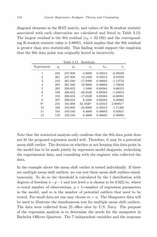
April 29, 2009 11:50 World Scientific Book - 9in x 6in Regression˙master
110 Linear Regression Analysis: Theory and Computing
diagonal elements in the HAT matrix, and values of the R-student statisticassociated with each observation are calculated and listed in Table 3.13.The largest residual is the 9th residual (e9 = 32.192) and the correspond-ing R-student statistic value is 2.86951, which implies that the 9th residualis greater than zero statistically. This finding would support the suspicionthat the 9th data point was originally keyed in incorrectly.
Table 3.13 Residuals
Experiment yi yi ei hii ti
1 243 247.808 -4.8080 0.45013 -0.292282 261 247.808 13.1920 0.45013 0.835943 244 261.040 -17.0400 0.46603 -1.137244 285 261.040 23.9600 0.46603 1.766485 202 200.652 1.3480 0.08384 0.063126 180 200.652 -20.6520 0.08384 -1.038547 183 200.652 -17.6520 0.08384 -0.869818 207 200.652 6.3480 0.08384 0.299049∗ 216 183.808 32.1920∗ 0.45013 2.86951∗
10 160 183.808 -23.8080 0.45013 -1.7140511 104 103.540 0.4600 0.46603 0.0282112 110 103.540 6.4600 0.46603 0.40062
Note that the statistical analysis only confirms that the 9th data point doesnot fit the proposed regression model well. Therefore, it may be a potentialmean shift outlier. The decision on whether or not keeping this data point inthe model has to be made jointly by regression model diagnosis, recheckingthe experimental data, and consulting with the engineer who collected thedata.
In the example above the mean shift outlier is tested individually. If thereare multiple mean shift outliers, we can test these mean shift outliers simul-taneously. To do so the threshold is calculated by the t distribution withdegrees of freedom n−p−1 and test level α is chosen to be 0.025/m, wheren=total number of observations, p + 1=number of regression parametersin the model, and m is the number of potential outliers that need to betested. For small data set one may choose m = n. The Manpower data willbe used to illustrate the simultaneous test for multiple mean shift outliers.The data were collected from 25 office sites by U.S. Navy. The purposeof the regression analysis is to determine the needs for the manpower inBachelor Officers Quarters. The 7 independent variables and the response

April 29, 2009 11:50 World Scientific Book - 9in x 6in Regression˙master
Multiple Linear Regression 111
variable y in the data set are
x1: Average daily occupancyx2: Monthly average numbers of check-insx3: Weekly hours of service desk operationx4: Square feet of common use areax5: Number of building wingsx6: Operational berthing capacityx7: Number of roomsy : Monthly man-hours
The data set is presented in Table 3.14:
Table 3.14 Manpower Data
Site x1 x2 x3 x4 x5 x6 x7 y
1 2.00 4.00 4 1.26 1 6 6 180.232 3.00 1.58 40 1.25 1 5 5 182.613 16.60 23.78 40 1.00 1 13 13 164.384 7.00 2.37 168 1.00 1 7 8 284.555 5.30 1.67 42.5 7.79 3 25 25 199.926 16.50 8.25 168 1.12 2 19 19 267.387 25.89 3.00 40 0 3 36 36 999.098 44.42 159.75 168 0.60 18 48 48 1103.249 39.63 50.86 40 27.37 10 77 77 944.21
10 31.92 40.08 168 5.52 6 47 47 931.8411 97.33 255.08 168 19.00 6 165 130 2268.0612 56.63 373.42 168 6.03 4 36 37 1489.5013 96.67 206.67 168 17.86 14 120 120 1891.7014 54.58 207.08 168 7.77 6 66 66 1387.8215 113.88 981.00 168 24.48 6 166 179 3559.9216 149.58 233.83 168 31.07 14 185 202 3115.2917 134.32 145.82 168 25.99 12 192 192 2227.7618 188.74 937.00 168 45.44 26 237 237 4804.2419 110.24 410.00 168 20.05 12 115 115 2628.3220 96.83 677.33 168 20.31 10 302 210 1880.8421 102.33 288.83 168 21.01 14 131 131 3036.6322 274.92 695.25 168 46.63 58 363 363 5539.9823 811.08 714.33 168 22.76 17 242 242 3534.4924 384.50 1473.66 168 7.36 24 540 453 8266.7725 95.00 368.00 168 30.26 9 292 196 1845.89
Data Source: Procedure and Analyses for Staffing Standards: Data Re-gression Analysis handbook (San Diego, California: Navy Manpower andMaterial Analysis Center, 1979).

April 29, 2009 11:50 World Scientific Book - 9in x 6in Regression˙master
112 Linear Regression Analysis: Theory and Computing
The SAS program for the simultaneous outlier detection is provided asfollows. In this example we choose m = n = 25 since data set is not toolarge and we can test all observations simultaneously in the data set.
proc reg data=manpow outest=out1 tableout;
model y=x1 x2 x3 x4 x5 x6 x7;
output out=out2
p=yhat r=e h=h RSTUDENT=t ;
run;
data out2; set out2;
cutoff=-quantile(’T’, 0.025/50, 25-8-1);
if abs(t)> cutoff then outlier="Yes";
else outlier="No";
run;
The output with information on multiple mean shift outliers is presentedin Table 3.15. Note that in this example we tested all data points (n = 25)simultaneously. The cutoff for identifying multiple mean shift outlier isα/2n = 0.025/25 quantile from the t distribution with degrees of freedomn − 1 − number of parameters = 25 − 1 − 8 = 16. In the output, “No”indicates that the corresponding observation is not a mean shift outlier and“Yes” means a mean shift outlier.
In Table 3.15, we detect outlier using all data points as a whole. Thisapproach is based on rather conservative Bonferroni inequality, i.e., set thecritical value to be tα/2n,n−p−1, where n is the total number of observationsto be tested and p is the total number of parameters in the regressionmodel. We use this approach in situation where individual outlier detectionand residual plot do not provide us enough information on model fitting.Detection of outlier as a whole may tell us that even individually thereis no evidence to identify an outlier, but as compare to other residuals inthe overall data set, one residual may be more extreme than other. Theidea behind this approach is that when we fit data to a model we wouldexpect the model can provide satisfactory fitted values for all data pointsas a whole.
In this example we set α = 0.05, n = 25, and p = 8. The cutoff for the teststatistic is
−tα/2n,n−p−1 = −t0.05/50,16 = 3.686155.

April 29, 2009 11:50 World Scientific Book - 9in x 6in Regression˙master
Multiple Linear Regression 113
Table 3.15 Simultaneous Outlier Detection
Obs yi yi ei hii ti Outlier
1 180.23 209.98 -29.755 0.25729 -0.07360 No2 182.61 213.80 -31.186 0.16088 -0.07257 No3 164.38 360.49 -196.106 0.16141 -0.45944 No4 284.55 360.11 -75.556 0.16311 -0.17621 No5 199.92 380.70 -180.783 0.14748 -0.41961 No6 267.38 510.37 -242.993 0.15890 -0.57043 No7 999.09 685.17 313.923 0.18288 0.75320 No8 1103.24 1279.30 -176.059 0.35909 -0.47199 No9 944.21 815.47 128.744 0.28081 0.32464 No
10 931.84 891.85 39.994 0.12954 0.09139 No11 2268.06 1632.14 635.923 0.12414 1.55370 No12 1489.50 1305.18 184.323 0.20241 0.44258 No13 1891.70 1973.42 -81.716 0.08020 -0.18179 No14 1387.82 1397.79 -9.966 0.09691 -0.02235 No15 3559.92 4225.13 -665.211 0.55760 -2.51918 No16 3115.29 3134.90 -19.605 0.40235 -0.05406 No17 2227.76 2698.74 -470.978 0.36824 -1.33105 No18 4804.24 4385.78 418.462 0.44649 1.25660 No19 2628.32 2190.33 437.994 0.08681 1.00741 No20 1880.84 2750.91 -870.070 0.36629 -2.86571 No21 3036.63 2210.13 826.496 0.07039 2.05385 No22 5539.98 5863.87 -323.894 0.78537 -1.60568 No23 3534.49 3694.77 -160.276 0.98846 -5.24234 Yes24 8266.77 7853.50 413.265 0.87618 3.20934 No25 1845.89 1710.86 135.029 0.54674 0.42994 No
We then compare the absolute value of each ti with this cutoff to determinewhether the corresponding observation is a possible outlier. Assuming thatthe regression model is correctly specified, the comparison between thiscutoff and each observation in the data set alerts that the 23th observationmight be an outlier.
The following example demonstrates the detection of multiple mean shiftoutliers. The magnitude of mean shift at different data point may be dif-ferent. The technique for multiple outlier detection is to create variableswhich take value 1 at these suspicious data point and 0 elsewhere. We needto create as many such columns as the number of suspicious outliers if webelieve there are different mean shifts at those data points. This way, wecan take care of different magnitudes of mean shift for all possible outliers.If we think some outliers are of the same mean shift then for these outlierwe should create a dummy variable that takes value 1 at these outliers and

April 29, 2009 11:50 World Scientific Book - 9in x 6in Regression˙master
114 Linear Regression Analysis: Theory and Computing
0 elsewhere.
In the following example, the data points with a larger value of variablex2 are suspicious and we would like to consider multiple data points 15,18, 22, 23, and 24 as possible multiple outliers. We first create 5 dummyvariables D1, D2, D3, D4, and D5 that takes value 1 at observations 15,18, 22, 23, and 24, and value 0 for all other observations in the data set.We then include these dummy variables in the regression model. The SASprogram for detecting the mean shift outliers is provided below.
data manpow; set manpow;
if _n_=15 then D15=1; else D15=0;
if _n_=18 then D18=1; else D18=0;
if _n_=22 then D22=1; else D22=0;
if _n_=23 then D23=1; else D23=0;
if _n_=24 then D24=1; else D24=0;
run;
Proc reg data=manpow;
model y=x1 x2 x3 x4 x5 x6 x7 D15 D18 D22 D23 D24;
run;
The output is presented in Table 3.16. The identified outlier is the 23thobservation since the corresponding P-value is 0.0160 < 0.05. Note that thistime we identified the same outlier via multiple outlier detection approach.
Table 3.16 Detection of Multiple Mean Shift Outliers
Variable df bi std ti P > |t|
Intercept 1 142.1511 176.0598 0.81 0.4351x1 1 23.7437 8.8284 2.69 0.0197x2 1 0.8531 0.8608 0.99 0.3412x3 1 -0.2071 1.7234 -0.12 0.9063x4 1 9.5700 16.0368 0.60 0.5618x5 1 12.7627 21.7424 0.59 0.5681x6 1 -0.2106 6.9024 -0.03 0.9762x7 1 -6.0764 12.5728 -0.48 0.6376Data15 1 723.5779 914.0654 0.79 0.4440Data18 1 139.5209 611.3666 0.23 0.8233Data22 1 -592.3845 900.1980 -0.66 0.5229Data23∗ 1 -15354 5477.3308 -2.80 0.0160∗
Data24 1 262.4439 1386.053 0.19 0.8530

April 29, 2009 11:50 World Scientific Book - 9in x 6in Regression˙master
Multiple Linear Regression 115
3.21 Check for Normality of the Error Term in MultipleRegression
We now discuss how to check normality assumption on error term of amultiple regression model. It is known that the sum of squared residuals,divided by n−p, is a good estimate of the error variance, where n is the totalnumber of observations and p is the number of parameters in the regressionmodel, The residual vector in a multiple linear regression is given by
e = (I −H)y = (I −H)(Xβ + ε) = (I −H)ε,
where H is the HAT matrix for this regression model. Each component
ei = εi −n∑
j=1
hijεj . Therefore, the normality of residual is not simply the
normality of the error term in the multiple regression model. Note that
Cov(e) = (I −H)σ2(I −H)′= (I −H)σ2.
Hence we can write Var(ei) = (1 − hii)σ2. If sample size is much largerthan the number of the model parameters, i.e., n >> p, or sample size n islarge enough, hii will be small as compared to 1, then Var(ei) ≈ σ2. Thus,a residual in multiple regression model behaves like error if sample size islarge. However, it is not true for small sample size. We point out thatit is unreliable to check normality assumption using the residuals from amultiple regression model when sample size is small.
3.22 Example
In this section we provide some illustrative examples of multiple regressionusing SAS. The following SAS program is for calculating confidence inter-vals on regression mean and regression prediction. The Pine Tree data setused in this example is presented in Table 3.17.
The corresponding estimated of regression parameters for the modelincluding all independent variables x1, x2, x3 and the model including x3, x2
are presented in Tables 3.18 and 3.19. The confidence intervals on regressionmean and regression prediction for the model including all variables and themodel including x1, x2 are presented in Tables 3.20 and 3.21.

April 29, 2009 11:50 World Scientific Book - 9in x 6in Regression˙master
116 Linear Regression Analysis: Theory and Computing
Table 3.17 Stand Characteristics of Pine TreeData
Age HD N MDBH
19 51.5 500 7.014 41.3 900 5.011 36.7 650 6.213 32.2 480 5.213 39.0 520 6.212 29.8 610 5.218 51.2 700 6.214 46.8 760 6.420 61.8 930 6.417 55.8 690 6.413 37.3 800 5.421 54.2 650 6.411 32.5 530 5.419 56.3 680 6.717 52.8 620 6.715 47.0 900 5.916 53.0 620 6.916 50.3 730 6.914 50.5 680 6.922 57.7 480 7.9
Data Source: Harold E, et al. “Yield of Old-fieldLoblolly Pine Plantations”, Division of Forestry andWildlife Resources Pub. FWS-3-72, Virginia Poly-technic Institute and State University, Blacksburg,Virginia, 1972.
data pinetree; set pinetree;
x1= HD;
x2=age*N;
x3=HD/N;
run;
proc reg data=pinetree outest=out tableout;
model MDBH=x1 x2 x3/all;
run;
*Calculation of partial sum;
proc reg data=pinetree;
model MDBH=x1 x2 x3;
run;

April 29, 2009 11:50 World Scientific Book - 9in x 6in Regression˙master
Multiple Linear Regression 117
Table 3.18 Parameter Estimates and Confidence Intervals Using x1, x2 and x3
MODEL TYPE DEPVAR RMSE Intercept x1 x2 x3
MODEL1 PARMS MDBH 0.29359 3.23573 0.09741 -0.00017 3.4668MODEL1 STDERR MDBH 0.29359 0.34666 0.02540 0.00006 8.3738MODEL1 T MDBH 0.29359 9.33413 3.83521 -2.79003 0.4140MODEL1 PVALUE MDBH 0.29359 0.00000 0.00146 0.01311 0.6844MODEL1 L95B MDBH 0.29359 2.50085 0.04356 -0.00030 -14.2848MODEL1 U95B MDBH 0.29359 3.97061 0.15125 -0.00004 21.2185
Table 3.19 Parameter Estimates and Confidence Intervals after Deleting x3
MODEL TYPE DEPVAR RMSE Intercept x1 x2
MODEL1 PARMS MDBH 0.28635 3.26051 0.1069 -0.00019MODEL1 STDERR MDBH 0.28635 0.33302 0.0106 0.00003MODEL1 T MDBH 0.28635 9.79063 10.1069 -5.82758MODEL1 PVALUE MDBH 0.28635 0.00000 0.0000 0.00002MODEL1 L95B MDBH 0.28635 2.55789 0.0846 -0.00026MODEL1 U95B MDBH 0.28635 3.96313 0.1292 -0.00012
proc reg data=pinetree outest=out tableout;
model MDBH=x1 x2;
run;
*Calculate fitted values and residuals;
proc reg data=pinetree;
model MDBH=x1 x2 x3;
output out=out p=yhat r=yresid student=sresid
LCLM=L_mean UCLM=U_mean
LCL=L_pred UCL=U_pred;
run;
*Calculate fitted values and residuals after deleting X3;
proc reg data=pinetree;
model MDBH=x1 x2;
output out=out p=yhat r=yresid student=sresid
LCLM=L_mean UCLM=U_mean
LCL=L_pred UCL=U_pred;
run;
If collinearity exists the regression analysis become unreliable. Although
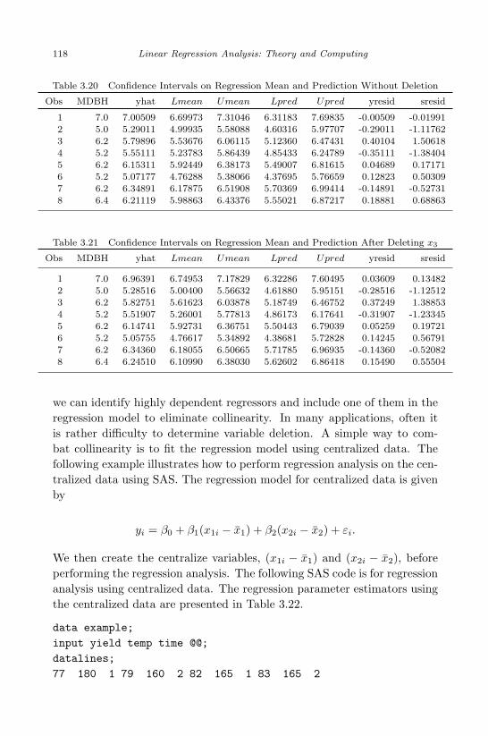
April 29, 2009 11:50 World Scientific Book - 9in x 6in Regression˙master
118 Linear Regression Analysis: Theory and Computing
Table 3.20 Confidence Intervals on Regression Mean and Prediction Without Deletion
Obs MDBH yhat Lmean Umean Lpred Upred yresid sresid
1 7.0 7.00509 6.69973 7.31046 6.31183 7.69835 -0.00509 -0.019912 5.0 5.29011 4.99935 5.58088 4.60316 5.97707 -0.29011 -1.117623 6.2 5.79896 5.53676 6.06115 5.12360 6.47431 0.40104 1.506184 5.2 5.55111 5.23783 5.86439 4.85433 6.24789 -0.35111 -1.384045 6.2 6.15311 5.92449 6.38173 5.49007 6.81615 0.04689 0.171716 5.2 5.07177 4.76288 5.38066 4.37695 5.76659 0.12823 0.503097 6.2 6.34891 6.17875 6.51908 5.70369 6.99414 -0.14891 -0.527318 6.4 6.21119 5.98863 6.43376 5.55021 6.87217 0.18881 0.68863
Table 3.21 Confidence Intervals on Regression Mean and Prediction After Deleting x3
Obs MDBH yhat Lmean Umean Lpred Upred yresid sresid
1 7.0 6.96391 6.74953 7.17829 6.32286 7.60495 0.03609 0.134822 5.0 5.28516 5.00400 5.56632 4.61880 5.95151 -0.28516 -1.125123 6.2 5.82751 5.61623 6.03878 5.18749 6.46752 0.37249 1.388534 5.2 5.51907 5.26001 5.77813 4.86173 6.17641 -0.31907 -1.233455 6.2 6.14741 5.92731 6.36751 5.50443 6.79039 0.05259 0.197216 5.2 5.05755 4.76617 5.34892 4.38681 5.72828 0.14245 0.567917 6.2 6.34360 6.18055 6.50665 5.71785 6.96935 -0.14360 -0.520828 6.4 6.24510 6.10990 6.38030 5.62602 6.86418 0.15490 0.55504
we can identify highly dependent regressors and include one of them in theregression model to eliminate collinearity. In many applications, often itis rather difficulty to determine variable deletion. A simple way to com-bat collinearity is to fit the regression model using centralized data. Thefollowing example illustrates how to perform regression analysis on the cen-tralized data using SAS. The regression model for centralized data is givenby
yi = β0 + β1(x1i − x1) + β2(x2i − x2) + εi.
We then create the centralize variables, (x1i − x1) and (x2i − x2), beforeperforming the regression analysis. The following SAS code is for regressionanalysis using centralized data. The regression parameter estimators usingthe centralized data are presented in Table 3.22.
data example;
input yield temp time @@;
datalines;
77 180 1 79 160 2 82 165 1 83 165 2
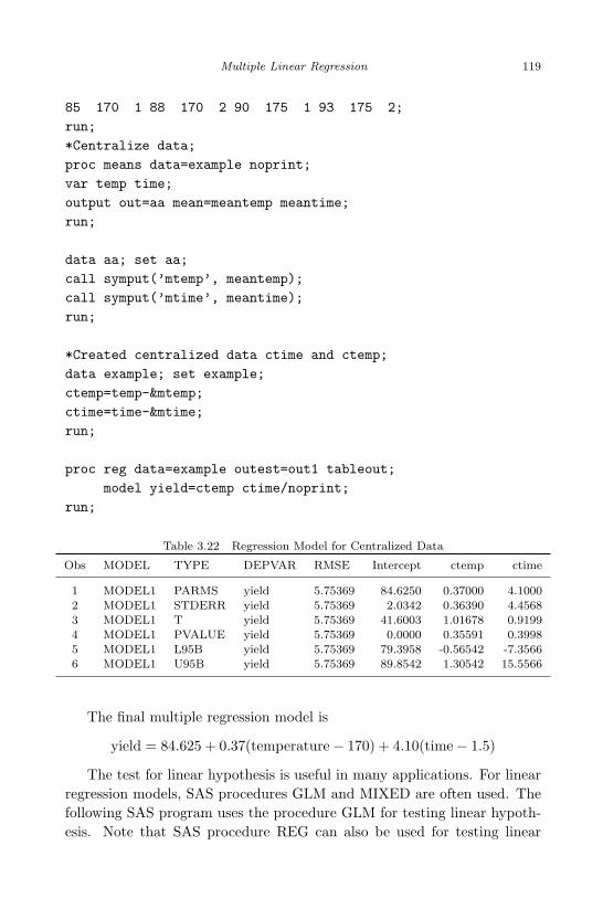
April 29, 2009 11:50 World Scientific Book - 9in x 6in Regression˙master
Multiple Linear Regression 119
85 170 1 88 170 2 90 175 1 93 175 2;
run;
*Centralize data;
proc means data=example noprint;
var temp time;
output out=aa mean=meantemp meantime;
run;
data aa; set aa;
call symput(’mtemp’, meantemp);
call symput(’mtime’, meantime);
run;
*Created centralized data ctime and ctemp;
data example; set example;
ctemp=temp-&mtemp;
ctime=time-&mtime;
run;
proc reg data=example outest=out1 tableout;
model yield=ctemp ctime/noprint;
run;
Table 3.22 Regression Model for Centralized Data
Obs MODEL TYPE DEPVAR RMSE Intercept ctemp ctime
1 MODEL1 PARMS yield 5.75369 84.6250 0.37000 4.10002 MODEL1 STDERR yield 5.75369 2.0342 0.36390 4.45683 MODEL1 T yield 5.75369 41.6003 1.01678 0.91994 MODEL1 PVALUE yield 5.75369 0.0000 0.35591 0.39985 MODEL1 L95B yield 5.75369 79.3958 -0.56542 -7.35666 MODEL1 U95B yield 5.75369 89.8542 1.30542 15.5566
The final multiple regression model is
yield = 84.625 + 0.37(temperature− 170) + 4.10(time− 1.5)
The test for linear hypothesis is useful in many applications. For linearregression models, SAS procedures GLM and MIXED are often used. Thefollowing SAS program uses the procedure GLM for testing linear hypoth-esis. Note that SAS procedure REG can also be used for testing linear
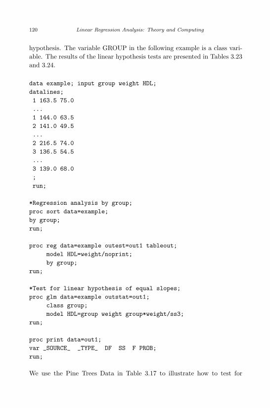
April 29, 2009 11:50 World Scientific Book - 9in x 6in Regression˙master
120 Linear Regression Analysis: Theory and Computing
hypothesis. The variable GROUP in the following example is a class vari-able. The results of the linear hypothesis tests are presented in Tables 3.23and 3.24.
data example; input group weight HDL;
datalines;
1 163.5 75.0
...
1 144.0 63.5
2 141.0 49.5
...
2 216.5 74.0
3 136.5 54.5
...
3 139.0 68.0
;
run;
*Regression analysis by group;
proc sort data=example;
by group;
run;
proc reg data=example outest=out1 tableout;
model HDL=weight/noprint;
by group;
run;
*Test for linear hypothesis of equal slopes;
proc glm data=example outstat=out1;
class group;
model HDL=group weight group*weight/ss3;
run;
proc print data=out1;
var _SOURCE_ _TYPE_ DF SS F PROB;
run;
We use the Pine Trees Data in Table 3.17 to illustrate how to test for

April 29, 2009 11:50 World Scientific Book - 9in x 6in Regression˙master
Multiple Linear Regression 121
Table 3.23 Test for Equal Slope Among 3 Groups
SOURCE TYPE DF SS F PROB
error error 20 1712.36group SS3 2 697.20 4.07157 0.03285weight SS3 1 244.12 2.85124 0.10684weight*group SS3 2 505.05 2.94946 0.07542
Table 3.24 Regression by Group
Group Model Type Depvar Rmse Intercept Weight
1 MODEL1 PARMS HDL 7.2570 23.054 0.249561 MODEL1 STDERR HDL 7.2570 25.312 0.157331 MODEL1 T HDL 7.2570 0.911 1.586291 MODEL1 PVALUE HDL 7.2570 0.398 0.163771 MODEL1 L95B HDL 7.2570 -38.883 -0.135401 MODEL1 U95B HDL 7.2570 84.991 0.634522 MODEL1 PARMS HDL 10.3881 14.255 0.250942 MODEL1 STDERR HDL 10.3881 17.486 0.117952 MODEL1 T HDL 10.3881 0.815 2.127412 MODEL1 PVALUE HDL 10.3881 0.446 0.077492 MODEL1 L95B HDL 10.3881 -28.532 -0.037692 MODEL1 U95B HDL 10.3881 57.042 0.539563 MODEL1 PARMS HDL 9.6754 76.880 -0.082133 MODEL1 STDERR HDL 9.6754 16.959 0.105143 MODEL1 T HDL 9.6754 4.533 -0.781163 MODEL1 PVALUE HDL 9.6754 0.002 0.457203 MODEL1 L95B HDL 9.6754 37.773 -0.324583 MODEL1 U95B HDL 9.6754 115.987 0.16032
linear hypothesis. The following SAS code test the linear hypothesis (a)H0: β0 = β1 = β2 = β3 = 0 versus H1: at least one βi 6= βj . (b) H0:β1 = β2 versus H1: β1 6= β2, both at a level 0.05 (default).
proc reg data=pinetree alpha=0.05;
model MDBH=x1 x2 x3;
test intercept=0,
x1=0,
x2=0,
x3=0;
test x1=x2;
run;

April 29, 2009 11:50 World Scientific Book - 9in x 6in Regression˙master
122 Linear Regression Analysis: Theory and Computing
The first hypothesis test (a) is the multiple test for checking if all parametersare zero and the observed value of the corresponding F test statistic is2302.95 with the p-value < .0001. Thus, we cannot confirm H0. For thesecond hypothesis test (b) the observed value of the corresponding F teststatistic is 14.69 with the p-value 0.0015. Since the p-value is less than thesignificance level we cannot confirm H0 either.Again, we use the Pine Trees Data to illustrate how to find the least squaresestimation under linear restrictions. The following SAS code compute theleast squares estimates under the linear restrictions β0 = 3.23 and β1 = β2.
proc reg data=pinetree;
model MDBH=x1 x2 x3;
restrict intercept=3.23, x1=x2/print;
run;
It is noted that the least squares estimates from the regression model with-out any linear restrictions are b0 = 3.2357, b1 = 0.09741, b2 = −0.000169and b3 = 3.4668. The least squares estimates with the linear restric-tions β0 = 3.23 and β1 = β2 are b0 = 3.23, b1 = b2 = 0.00005527 andb3 = 33.92506.
Problems
1. Using the matrix form of the simple linear regression to show the un-biasness of the b. Also, calculate the covariance of b using the matrixformat of the simple linear regression.
2. Let X be a matrix of n ×m and X = (X1, X2), where X1 is n × k
matrix and X2 is n× (m− k) matrix. Show that
(a). The matrices X(X′X)−1X
′and X1(X
′1X1)−1X
′1 are idempo-
tent.(b). The matrix X(X
′X)−1X
′ −X2(X′2X2)−1X
′2 is idempotent.
(c). Find the rank of the matrix X(X′X)−1X
′ −X2(X′2X2)−1X
′2.
3. The least squares estimators of the regression model Y = Xβ + ε arelinear function of the y-observations. When (X
′X)−1 exists the least
squares estimators of β is b = (X′X)−1Xy. Let A be a constant
matrix. Using Var(Ay) = AVar(y)A′
and Var(y) = σ2I to show thatVar(b) = σ2(X
′X)−1.

April 29, 2009 11:50 World Scientific Book - 9in x 6in Regression˙master
Multiple Linear Regression 123
4. Show that the HAT matrix in linear regression model has the propertytr(H) = p where p is the total numbers of the model parameters.
5. Let hii be the ith diagonal elements of the HAT matrix. Prove that
(a). For a multiple regression model with a constant term hii ≥ 1/n.(b). Show that hii ≤ 1. (Hint: Use the fact that the HAT matrix is
idempotent.)
6. Assume that the data given in Table 3.25 satisfy the model
yi = β0 + β1x1i + β2x2i + εi,
where εi’s are iid N(0, σ2).
Table 3.25 Data Set for Calculation of Confidence Interval on Regression Prediction
y 12.0 11.7 9.3 11.9 11.8 9.5 9.3 7.2 8.1 8.3 7.0 6.5 5.9
x1 3 4 5 6 7 8 9 10 11 12 13 14 15x2 6 4 2 1 0 1 2 1 -1 0 -2 -1 -3
Data Source: Franklin A. Grabill, (1976), Theory and Application of the linear model.p. 326.
(a). Find 80 percent, 90 percent, 95 percent, and 99 percent confidenceinterval for y0, the mean of one future observation at x1 = 9.5 andx2 = 2.5.
(b). Find a 90 percent confidence interval for y0, the mean of six ob-servations at x1 = 9.5 and x2 = 2.5.
7. Consider the general linear regression model y = Xβ + ε and the leastsquares estimate b = (X
′X)−1X
′y. Show that
b = β + Rε,
where R = (X′X)−1X
′.
8. A scientist collects experimental data on the radius of a propellant grain(y) as a function of powder temperature, x1, extrusion rate, x2, anddie temperature, x3. The data is presented in Table 3.26.
(a). Consider the linear regression model
yi = β?0 + β1(x1i − x1) + β2(x2i − x2) + β3(x3i − x3) + εi.
Write the vector y, the matrix X, and vector β in the modely = Xβ + ε.
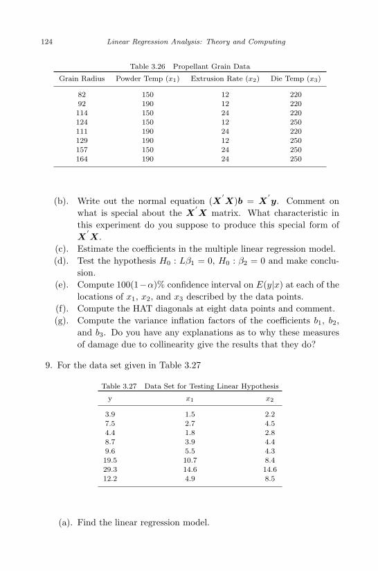
April 29, 2009 11:50 World Scientific Book - 9in x 6in Regression˙master
124 Linear Regression Analysis: Theory and Computing
Table 3.26 Propellant Grain Data
Grain Radius Powder Temp (x1) Extrusion Rate (x2) Die Temp (x3)
82 150 12 22092 190 12 220114 150 24 220124 150 12 250111 190 24 220129 190 12 250157 150 24 250164 190 24 250
(b). Write out the normal equation (X′X)b = X
′y. Comment on
what is special about the X′X matrix. What characteristic in
this experiment do you suppose to produce this special form ofX
′X.
(c). Estimate the coefficients in the multiple linear regression model.(d). Test the hypothesis H0 : Lβ1 = 0, H0 : β2 = 0 and make conclu-
sion.(e). Compute 100(1−α)% confidence interval on E(y|x) at each of the
locations of x1, x2, and x3 described by the data points.(f). Compute the HAT diagonals at eight data points and comment.(g). Compute the variance inflation factors of the coefficients b1, b2,
and b3. Do you have any explanations as to why these measuresof damage due to collinearity give the results that they do?
9. For the data set given in Table 3.27
Table 3.27 Data Set for Testing Linear Hypothesis
y x1 x2
3.9 1.5 2.27.5 2.7 4.54.4 1.8 2.88.7 3.9 4.49.6 5.5 4.319.5 10.7 8.429.3 14.6 14.612.2 4.9 8.5
(a). Find the linear regression model.

April 29, 2009 11:50 World Scientific Book - 9in x 6in Regression˙master
Multiple Linear Regression 125
(b). Use the general linear hypothesis test to test
H0 : β1 = β2 = 0
and make your conclusion. Use full and restricted model residualsums of squares.
10. Consider the general linear regression model y = Xβ + ε and the leastsquares estimate b = (X
′X)−1X
′y. Show that
b = β + Rε,
where R = (X′X)−1X
′.
11. In an experiment in the civil engineering department of Virginia Poly-technic Institute and State University in 1988, a growth of certain typeof algae in water was observed as a function of time and dosage ofcopper added into the water. The collected data are shown in Table3.28.
(a). Consider the following regression model
yi = β0 + β1x1i + β2x2i + β12x1ix2i + εi
Estimate the coefficients of the model, using multiple linear re-gression.
(b). Test H0 : β12 = 0 versus H1 : β12 6= 0. Do you have any reason tochange the model given in part (a).
(c). Show a partitioning of total degrees of freedom into those at-tributed to regression, pure error, and lack of fit.
(d). Using the model you adopted in part (b), make a test for lack offit and draw conclusion.
(e). Plot residuals of your fitted model against x1 and x2 separately,and comment.

April 29, 2009 11:50 World Scientific Book - 9in x 6in Regression˙master
126 Linear Regression Analysis: Theory and Computing
Table 3.28 Algae Data
y(unit of algae) x1(copper, mg) x2(days)
.3 1 5.34 1 5.2 2 5.24 2 5.24 2 5.28 3 5.2 3 5.24 3 5.02 4 5.02 4 5.06 4 50 5 50 5 50 5 5
.37 1 12
.36 1 12
.30 2 12
.31 2 12
.30 2 12
.30 3 12
.30 3 12
.30 3 12
.14 4 12
.14 4 12
.14 4 12
.14 5 12
.15 5 12
.15 5 12
.23 1 18
.23 1 18
.28 2 18
.27 2 18
.25 2 18
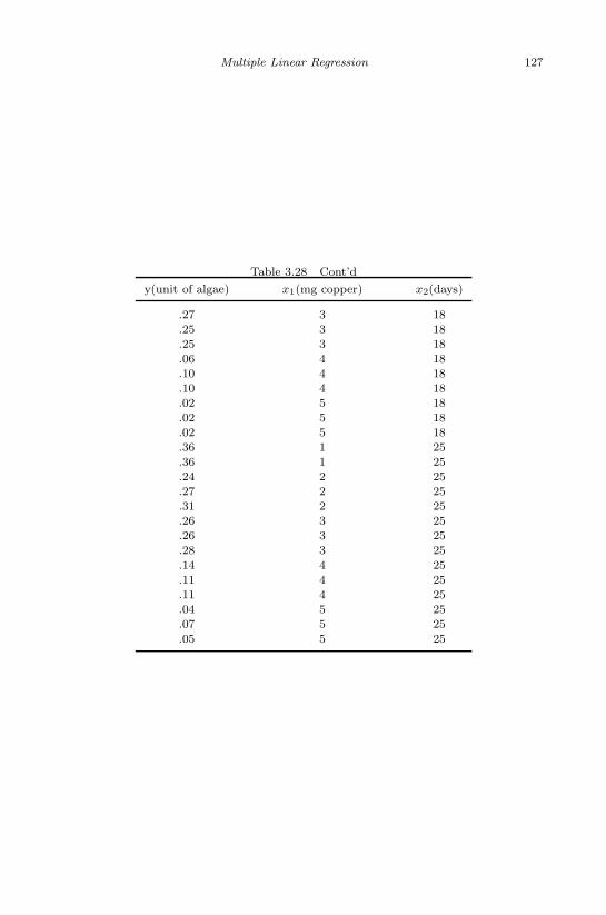
May 7, 2009 10:22 World Scientific Book - 9in x 6in Regression˙master
Multiple Linear Regression 127
Table 3.28 Cont’d
y(unit of algae) x1(mg copper) x2(days)
.27 3 18
.25 3 18
.25 3 18
.06 4 18
.10 4 18
.10 4 18
.02 5 18
.02 5 18
.02 5 18
.36 1 25
.36 1 25
.24 2 25
.27 2 25
.31 2 25
.26 3 25
.26 3 25
.28 3 25
.14 4 25
.11 4 25
.11 4 25
.04 5 25
.07 5 25
.05 5 25

April 29, 2009 11:50 World Scientific Book - 9in x 6in Regression˙master
This page intentionally left blankThis page intentionally left blank

April 29, 2009 11:50 World Scientific Book - 9in x 6in Regression˙master
Chapter 4
Detection of Outliers and InfluentialObservations in Multiple Linear
Regression
After data is collected, and cleaned the next step is to fit the data to aselected statistical model so that the relationship between response variableand independent variables may be established. Choosing a statistical modellargely depends on the nature of data from the experiment and the scientificquestions that need to be answered. If linear regression model is selected,determination of the model is to solve for the regression parameters. Afterthat it is needed to perform hypothesis tests for those parameters and it isnecessary to perform model diagnosis.
We have already stated that for classical regression model the methodfor solving regression parameters is the least squares method. If the errorterm in the regression model is normally distributed the least squares esti-mates of the regression parameters are the same as the maximum likelihoodestimates. After the estimates of the linear regression model are obtained,the next question is to answer whether or not this linear regression modelis reasonably and adequately reflect the true relationship between responsevariable and independent variables. This falls into the area of regressiondiagnosis. There are two aspects of the regression diagnosis. One is tocheck if a chosen model is reasonable enough to reflect the true relation-ship between response variable and independent variables. Another is tocheck if there are any data points that deviate significantly from the as-sumed model. The first question belongs to model diagnosis and the secondquestion is to check outliers and influential observations. We focus on thedetection of outliers and influential observations in this section.
Identifying outliers and influential observations for a regression modelis based on the assumption that the regression model is correctly specified.That is, the selected regression model adequately specifies the relationshipbetween response variable and independent variables. Any data points that
129
April 29, 2009 11:50 World Scientific Book - 9in x 6in Regression˙master
130 Linear Regression Analysis: Theory and Computing
fit well the assumed model are the right data points for the assumed model.Sometimes, however, not all data points fit the model equally well. Theremay be some data points that may deviate significantly from the assumedmodel. These data points may be considered as outliers if we believe thatthe selected model is correct. Geometrically, linear regression is a line(for simple linear regression) or a hyperplane (for multiple regression). Ifa regression model is appropriately selected, most data points should befairly close to regression line or hyperplane. The data points which are faraway from regression line or hyperplane may not be “ideal” data points forthe selected model and could potentially be identified as the outliers forthe model. An outlier is the data point that is statistically far away fromthe chosen model if we believe that the selected regression model is correct.An influential observation is one that has a relatively larger impact on theestimates of one or more regression parameters. i.e., including or excludingit in the regression model fitting will result in unusual change in one ormore estimates of regression parameters. We will discuss the statisticalprocedures for identifying outliers and influential observations.
4.1 Model Diagnosis for Multiple Linear Regression
4.1.1 Simple Criteria for Model Comparison
Before checking a regression model, one has to understand the following:
• Scientific questions to be answered• Experiment from which the data is collected• Statistical model and model assumptions
It should be understood that the model selection may be rather complicatedand sometimes it is difficult to find a “perfect model” for your data. DavidR. Cox made famous comment on model selection, “all models are wrong,but some are useful”. This implies that no “optimal scheme” is ever inpractice optimal. The goal of statistical modeling is to find a reasonableand useful model upon which we can answer desired scientific questionsbased on data obtained from well-designed scientific experiment. This canbe done through model comparison. The following are some basic criteriathat are commonly used for regression model diagnosis:
1. Coefficients of determination R2 = 1− SSRes
SSTotal. The preferred model
April 29, 2009 11:50 World Scientific Book - 9in x 6in Regression˙master
Detection of Outliers and Influential Observations in Multiple Linear Regression 131
would be the model with R2 value close to 1. If the data fit well theregression model then it should be expected that yi is close enough toyi. Hence, SSRes should be fairly close to zero. Therefore, R2 shouldbe close to 1.
2. Estimate of error variance s2. Among a set of possible regression modelsa preferred regression model should be one that has a smaller value ofs2 since this corresponds to the situation where the fitted values arecloser to the response observations as a whole.
3. Adjusted R2. Replace SSRes and SSTotal by their means:
R2 = 1− SSRes/n− p
SSTotal/n− 1= 1− s2(n− 1)
SSTotal
Note that SSTotal is the same for all models and the ranks of R2 for allmodels are the same as the ranks of s2 for all models. We would liketo choose a regression model with adjusted R2 close to 1.
4.1.2 Bias in Error Estimate from Under-specified Model
We now discuss the situation where the selected model is under-specified.i.e.,
y = X1β1 + ε. (4.1)
Here, the under-specified model is a model with inadequate regressors. Inother words, if more regressors are added into the model, the linear com-bination of the regressors can better predict the response variable. Some-times, the under-specified model is also called as reduced model. Assumingthat the full model is
y = X1β1 + X2β2 + ε, (4.2)
and the number of parameters in the reduced model is p, let s2p be the error
estimate based on the under-specified regression model. The fitted valuefrom the under-specified regression model is
y = X1(X′1X1)−1X
′1y
and error estimate from the under-specified regression model is
s2p = y
′(I −X1(X
′1X1)−1X
′1)y.
We then compute the expectation of the error estimate s2p.
E(s2p) = σ2 +
β′2[X
′2X2 −X
′2X1(X
′1X1)−1X
′2X1]β2
n− p. (4.3)

April 29, 2009 11:50 World Scientific Book - 9in x 6in Regression˙master
132 Linear Regression Analysis: Theory and Computing
The above derivations need to use the formula of inverse matrix of par-titioned matrix and the fact that E(y) = X1β1 + X2β2. Note that s2
p
based on the under-specified regression model is a biased estimate of theerror variance. The bias due to under-specification of a regression model isa function of deleted parameters β2 and its covariance matrix.
4.1.3 Cross Validation
Suppose that yi is the ith response and (xi1, xi2, · · · , xip) is the ith regressorobservation vector. The data can be written in the following matrix format:
(y,X) =
y1 x1,1 · · · x1,p
y2 x2,1 · · · x2,p
...yn1 xn11 · · · xn1,p
yn1+1 xn1+1,1 · · · xn1+1,p
...yn xn,1 · · · xn,p
=(
y1 X1
y2 X2
), (4.4)
where 1 < n1 < n. The cross validation approach is to select n1 datapoints out of n data points to fit regression model and use the rest n− n1
data points to assess the model. This way, the first n1 data points serve asthe learning sample and the remaining n − n1 data points are the testingsample. To assess the model using the rest n− n1 data points we use sumof prediction errors
∑ni=n1+1(yi − yi)2 as assessment criterion. Note that
the prediction yi is computed using the regression model from the first n1
data points and the observations in the remaining n− n1 data points. Theidea behind this model checking approach is that the model parameters areobtained using the first n1 data points. If this is an appropriate model forthe whole data set then it should also yield a smaller value of the sum ofthe squared prediction errors from the remaining n−n1 observations. Notethat this criterion is harder than the criterion we have previously discussed,where the mean square error criterion is used rather than the criterion ofprediction error. Furthermore, it should be noted that the prediction hasa larger variance than the fitted value.
The above cross validation approach can be modified by randomlychoosing a subset of size ν to fit a regression model, then the remaining n−ν
data points are used to calculate the prediction error. This can be donek times, where k is a pre-defined integer. Suppose that β1, β2, · · · , βk are
April 29, 2009 11:50 World Scientific Book - 9in x 6in Regression˙master
Detection of Outliers and Influential Observations in Multiple Linear Regression 133
the least squares estimates each uses the randomly selected ν data points.We can use the average β = 1
k
∑ki=1 βi as the estimate of the regression
parameters and check the regression model using the average predictionerrors. This average of prediction errors can be used as the criterion ofregression model diagnosis. This technique is called ν-fold cross validationmethod and is often better than the cross validation method of choosingonly one subset as a learning sample.
When the cross validation approach is used, the entire data set is splitinto learning sample and testing sample to fit the regression model andto test the regression model. If selected regression model is appropriatethrough model checking using the testing samples mentioned above, thefinal regression model parameters should be estimated by the entire dataset. Finally, studied by Snee (1977), as a rule of thumb, the total numberof observations required for applying the cross validation approach is n ≥2p + 20, where p is the number of parameters in the regression model.
4.2 Detection of Outliers in Multiple Linear Regression
If the difference between fitted value yi and response yi is large, we may sus-pect that the ith observation is a potential outlier. The purpose of outlierdetection in regression analysis is tempted to eliminate some observationsthat have relatively larger residuals so that the model fitting may be im-proved. However, eliminating observations cannot be made solely basedon statistical procedure. Determination of outlier should be made jointlyby statisticians and subject scientists. In many situations, eliminating ob-servations is never made too easy. Some observations that do not fit themodel well may imply a flaw in the selected model and outlier detectionmight actually result in altering the model.
Regression residuals carry the most useful information for model fitting.There are two types of residuals that are commonly used in the outlierdetection: the standardized residual and the studentized residual.
Definition 4.1. Let s be the mean square error of a regression model. Thestandardized residual is defined as
zi =yi − yi
s(4.5)
The standardized residual is simply the normalized residual or the z-scoreof the residual.

April 29, 2009 11:50 World Scientific Book - 9in x 6in Regression˙master
134 Linear Regression Analysis: Theory and Computing
Definition 4.2. Let s be the mean square error of a regression model. Thestudentized residual is defined as
zi =yi − yi
s√
1− hii
(4.6)
where hii is the ith diagonal element of the HAT matrix (also called lever-age). The studentized residuals are so named because they follow approxi-mately the t-distribution.
According to Chebyshev’s inequality, for any random variable X, if E(X)exists, P (|X − E(X)| ≤ kσ) ≥ 1 − 1/k2. If k = 3, the probability of arandom variable within 3 times of standard deviation from its mean is notless than 1− 1/32 = 8/9 ≈ 88.9%. One would like to define an observationas a potential outlier if it is 3 times of the standard deviation away fromits mean value.
Definition 4.3. If the residual of an observation is larger than 3 times ofthe standard deviation (or standardized residual is larger than 3) then theobservation may be considered as an outlier.
Note that this outlier definition considers outlier individually. If we con-sider multiple outliers simultaneously then the simplest way is to use t-distribution and the Bonferroni multiplicity adjustment.
4.3 Detection of Influential Observations in Multiple LinearRegression
4.3.1 Influential Observation
It is known that data points may have different influences on the regressionmodel. Different influences mean that some data points may have largerimpact on the estimates of regression coefficients than that of other datapoints.
An influential observation is the data point that causes a significant changein the regression parameter estimates if it is deleted from the whole dataset. Based on this idea we remove one observation at a time to fit the sameregression model then calculate the fitted value yi,−i from the regressionmodel without using the ith data point. The fitted value of y without usingthe ith data point is defined as
yi,−i = xib−i,

April 29, 2009 11:50 World Scientific Book - 9in x 6in Regression˙master
Detection of Outliers and Influential Observations in Multiple Linear Regression 135
where xi is the ith regressor vector, and b−i is the least squares estimatebased on the same regression model using all data points except for theresponse yi and the regressor vector xi. To measure the difference betweenresponse yi and yi,−i we introduce the following PRESS residual.
Definition 4.4. The PRESS residual is defined as
ei,−i = yi − yi,−i (4.7)
The PRESS residual measures the impact of the ith observation on theregression model. An observation with a larger PRESS residual may bea possible influential observation. i.e., the fitted regression model basedon the data excluding this observation is quite different from the fittedregression model based on the data including this observation. The sum ofthe squared PRESS residuals is defined as the PRESS statistic.
Definition 4.5. The PRESS statistic is defined as
PRESS =n∑
i=1
(yi − yi,−i)2 =n∑
i=1
(ei,−i)2 (4.8)
The PRESS residual can be expressed by the usual residual. It can beshown that
PRESS =n∑
i=1
(ei,−i)2
=n∑
i=1
( yi − yi
1− x′i(X
′X)−1xi
)2
=n∑
i=1
( ei
1− hii
)2
, (4.9)
where hii is the ith diagonal element of the HAT matrix. This relationshipmakes calculation of the PRESS residual easier. Note that hii is always be-tween 0 and 1. If hii is small (close to 0), even a larger value of the ordinaryresidual ei may result in a smaller value of the PRESS residual. If hii islarger (close to 1), even a small value of residual ei could result in a largervalue of the PRESS residual. Thus, an influential observation is determinednot only by the magnitude of residual but also by the corresponding valueof leverage hii.
The PRESS statistic can be used in the regression model selection. A betterregression model should be less sensitive to each individual observation. Inother words, a better regression model should be less impacted by excludingone observation. Therefore, a regression model with a smaller value of thePRESS statistic should be a preferred model.

May 7, 2009 10:22 World Scientific Book - 9in x 6in Regression˙master
136 Linear Regression Analysis: Theory and Computing
4.3.2 Notes on Outlier and Influential Observation
What is outlier? If there is breakdown in the model at the ith data pointsuch that the mean is shifted. Typically, it is the phenomenon that E(εi) =∆ = 0. i.e., there is a mean shift for the ith observation. If we believe thatthe regression model is correctly specified, the ith observation may be apossible outlier when there is a mean shift at the ith observation.
Another aspect of an outlier is that the variance of ε is larger at the ithobservation. i.e., there might be an inflation in variance at ith observa-tion. If we believe that equal variance assumption is appropriate, the ithobservation may be a potential outlier when its variance is inflated. So,an outlier could be examined by looking at both mean shift and varianceinflation at a particular data point. In addition, the ith PRESS residualei,−i = yi − yi,−i can be used to determine outlier in regression model. Ifthere is a mean shift at the ith data point, then we have
E(yi − yi,−i) = ∆i.
Similarly, if there is a variance inflation at the ith data point we would liketo use the standardized PRESS residual
ei,−i
σi,−i=
ei
σ√
1− hii
(4.10)
to detect a possible outlier. Since σ is unknown, we can replace σ by itsestimate s in the calculation of the standardized PRESS residual. However,in the presence of a mean shift outlier s is not an ideal estimate of truestandard deviation of σ.
If there is a mean shift outlier at the ith observation, then s is biasedupward. Hence, s is not an ideal estimate of σ. One way to deal withthis situation is to leave the ith observation out and calculate the standarddeviation with using the ith observation, denoted by s−i. s−i can be easilycalculated based on the relationship between s−i and s:
s−i =
√(n− p)s2 − e2
i /(1− hii)n− p− 1
. (4.11)
If equal variance assumption is suspicious for a regression model, we canuse the generalized least squares estimate where the equal variance assump-tion is not required. To conclude the discussion on outlier and influential

April 29, 2009 11:50 World Scientific Book - 9in x 6in Regression˙master
Detection of Outliers and Influential Observations in Multiple Linear Regression 137
observation in regression model, we point out that each observation can beexamined under the following four groups.
(1). Usual observation: this is the observation which has equal effects onthe fitted values. Regression model will not be affected with or withoutthis observation. This type of observations should be used to estimatethe model parameters.
(2). Outlier: an outlier is an observation for which the studentized residualis large in magnitude as compared to the studentized residuals of otherobservations in the data set. Outlier may indicate the violation ofmodel assumptions or may imply the need for an alternative model.
(3). High leverage point: it is an observation which is far from the centerof X space compared to other observations. Note that the concept ofleverage is only related to the regressors, not the response variable.
(4). Influential observation: influential observation is the observation thathas more impact on the regression coefficients or the estimate of vari-ance as compared to other observations in the data set.
The relationship among outlier, influential observation, and high-leverage observation can be summarized as follows:
(1). An outlier needs not be an influential observation.(2). An influential observation need not be an outlier.(3). There is a tendency for a high-leverage observation to have small resid-
uals and to influence the regression fit disproportionately.(4). A high-leverage observation may not necessarily be an influential ob-
servation and an influential observation may not necessarily be a high-leverage observation.
(5). An observation might be an outlier, a high-leverage point, or an influ-ential observation, simultaneously.
4.3.3 Residual Mean Square Error for Over-fitted Regres-
sion Model
In this section we discuss the consequence of under-fitting and over-fittingin regression analysis. Let’s assume that the correct model should includeall regressors X1 and X2, where X1 and X2 have p1 and p2 independentvariables, respectively. We thus write the following full regression model:
y = X1β1 + X2β2 + ε.
April 29, 2009 11:50 World Scientific Book - 9in x 6in Regression˙master
138 Linear Regression Analysis: Theory and Computing
Assume that the under-fitted model only includes X1 and is given by
y = X1β1 + ε∗.
In other words, an under-fitted regression model is the model from whichsome necessary regressors are omitted. Based on the under-fitted model wecan solve for the least squares estimate of β1:
b1 = (X′1X1)−1X
′1y.
It can be verified that b1 is a biased estimate of β1:
E(b1) = (X′1X1)−1X
′1E(y)
= (X′1X1)−1X
′1(X1β1 + X2β2)
= β1 + (X′1X1)−1X
′1X2β2
= β1 + Aβ2.
Thus, an under-fitted model has a bias (X′1X1)−1X
′1X2β2. Suppose that
we over-fit a regression model with m parameters
y = X1β1 + X2β2 + ε
when the right model would be the one with β2 = 0. The residual meansquare of the over-fitted model is
s2m =
y′(I −X(X
′X)−1X)y
n−m. (4.12)
We have
E(s2m) = σ2 +
1n−m
β′1X
′1(I −X(X
′X)−1X)X1β1. (4.13)
It is known that the linear space spanned by the columns of (I −X(X
′X)−1X) is perpendicular to the linear space spanned by the column
X, therefore, to the linear space spanned by the columns of X1. Thus, wehave
X′1(I −X(X
′X)−1X)X1 = 0.

April 29, 2009 11:50 World Scientific Book - 9in x 6in Regression˙master
Detection of Outliers and Influential Observations in Multiple Linear Regression 139
This yields E(s2m) = σ2 which implies that s2
m is an unbiased estimateof the true variance σ2 regardless of over-fitting. Furthermore, under thenormality assumption of the model error term we have
(n−m)s2m
σ2∼ χ2
n−m. (4.14)
According to the χ2 distribution we have
Var(s2m) =
σ4
(n−m)2Var(χ2
n−m) =2σ4
n−m. (4.15)
Note that if the model is over-fitted the degrees of freedom is n−m, whichis smaller than that from an ideal regression model. Therefore, for an over-fitted regression model, even s2
m is an unbiased estimate of the true varianceσ2, the variance of s2
m tends to be larger. We will further discuss the effectof under-fitting and over-fitting for multiple regression model in the nextchapter.
4.4 Test for Mean-shift Outliers
When the ith observation is suspected to be an outlier, we can consider theso-called mean-shift outlier model
y = Xβ + eiγ + ε, (4.16)
where ei denotes the ith n × 1 unit vector. The problem to test whetheror not the ith observation is a possible outlier can be formulated into thefollowing hypothesis testing problem in the mean-shift outlier model:
H0 : γ = 0 versus H1 : γ 6= 0.
We now discuss how to test mean shift outlier individually using the t-teststatistic. When the ith observation is a potential mean shift outlier s2 is abiased estimate of the error variance σ2; therefore, we would prefer to usethe leave-one-out s−i and replacing σ by s−i to construct the following teststatistic
ti =yi − yi
s−i
√1− hii
∼ tn−p−1. (4.17)
Under the null hypothesis H0 : ∆i = 0, the above test statistic has thecentralized t distribution with degrees of freedom of n − p − 1. It can be

May 7, 2009 10:22 World Scientific Book - 9in x 6in Regression˙master
140 Linear Regression Analysis: Theory and Computing
used to test the hypothesis H0 : ∆i = 0 versus the alternative H1 : ∆i = 0.The above statistic is often called the R-student statistic. It tends to belarger if the ith observation is a mean shift outlier. Note that the two-tailedt-test should be used. The rejection of H0 implies that the ith observationmay be a possible mean shift outlier. Note also that this test requires priorknowledge about a chosen observation being a potential outlier. If suchknowledge is not available, then we can weaken the alternative hypothesisto “there is at least one outlier in the model”. One may use the test statistic
tmax = max1≤i≤n
ti
and reject the null hypothesis H0 at level α if
|tmax| = | max1≤i≤n
ti| > tn−p−1, α/2n. (4.18)
This is equivalent to testing each individual observation and rejecting thenull hypothesis if at least one test is significant. Note that we have to choosethe test level to be α/n, which is the Bonferroni multiplicity adjustment,in order to ensure that the probability of the Type I error for the overalltest is bounded by α.
The R-student statistic can also be used to test variance inflation at the ithobservation. If there is a variance inflation at the ith observation then weshould have Var(εi) = σ2 + σ2
i . Here σ2i represents the increase in variance
at ith observation. The hypothesis is H0 : σ2i = 0 versus H1 : σ2
i = 0. Notethat the two-tailed t-test should be used.
We use the following example to illustrate how to compute R-student statis-tic to test mean shift outlier. The Coal-cleansing Data is used in the exam-ple. There are 3 variables in the data set. Variable x1 is the percent solidsin the input solution; x2 is the pH of the tank that holds the solution; andx3 is the flow rate of the cleansing polymer in ml/minute. The responsevariable y is the polymer used to clean coal and suspended solids (mg/l).There are a total of 15 experiments performed. The data set is presentedin Table 4.1.
proc reg data=coal outest=out1 tableout;
model y=x1 x2 x3;
output out=out2
p=yhat r=yresid h=h RSTUDENT=rstudent;
run;
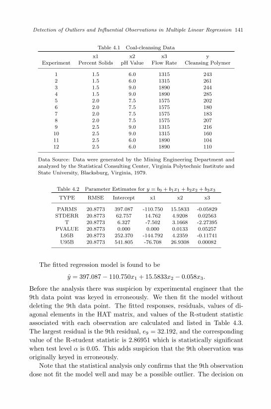
April 29, 2009 11:50 World Scientific Book - 9in x 6in Regression˙master
Detection of Outliers and Influential Observations in Multiple Linear Regression 141
Table 4.1 Coal-cleansing Data
x1 x2 x3 yExperiment Percent Solids pH Value Flow Rate Cleansing Polymer
1 1.5 6.0 1315 2432 1.5 6.0 1315 2613 1.5 9.0 1890 2444 1.5 9.0 1890 2855 2.0 7.5 1575 2026 2.0 7.5 1575 1807 2.0 7.5 1575 1838 2.0 7.5 1575 2079 2.5 9.0 1315 21610 2.5 9.0 1315 16011 2.5 6.0 1890 10412 2.5 6.0 1890 110
Data Source: Data were generated by the Mining Engineering Department andanalyzed by the Statistical Consulting Center, Virginia Polytechnic Institute andState University, Blacksburg, Virginia, 1979.
Table 4.2 Parameter Estimates for y = b0 + b1x1 + b2x2 + b3x3
TYPE RMSE Intercept x1 x2 x3
PARMS 20.8773 397.087 -110.750 15.5833 -0.05829STDERR 20.8773 62.757 14.762 4.9208 0.02563
T 20.8773 6.327 -7.502 3.1668 -2.27395PVALUE 20.8773 0.000 0.000 0.0133 0.05257
L95B 20.8773 252.370 -144.792 4.2359 -0.11741U95B 20.8773 541.805 -76.708 26.9308 0.00082
The fitted regression model is found to be
y = 397.087− 110.750x1 + 15.5833x2 − 0.058x3.
Before the analysis there was suspicion by experimental engineer that the9th data point was keyed in erroneously. We then fit the model withoutdeleting the 9th data point. The fitted responses, residuals, values of di-agonal elements in the HAT matrix, and values of the R-student statisticassociated with each observation are calculated and listed in Table 4.3.The largest residual is the 9th residual, e9 = 32.192, and the correspondingvalue of the R-student statistic is 2.86951 which is statistically significantwhen test level α is 0.05. This adds suspicion that the 9th observation wasoriginally keyed in erroneously.
Note that the statistical analysis only confirms that the 9th observationdose not fit the model well and may be a possible outlier. The decision on

April 29, 2009 11:50 World Scientific Book - 9in x 6in Regression˙master
142 Linear Regression Analysis: Theory and Computing
Table 4.3 Residuals, Leverage, and ti
Experiment yi yi ei hii ti
1 243 247.808 -4.8080 0.45013 -0.292282 261 247.808 13.1920 0.45013 0.835943 244 261.040 -17.0400 0.46603 -1.137244 285 261.040 23.9600 0.46603 1.766485 202 200.652 1.3480 0.08384 0.063126 180 200.652 -20.6520 0.08384 -1.038547 183 200.652 -17.6520 0.08384 -0.869818 207 200.652 6.3480 0.08384 0.299049∗ 216 183.808 32.1920∗ 0.45013 2.86951∗
10 160 183.808 -23.8080 0.45013 -1.7140511 104 103.540 0.4600 0.46603 0.0282112 110 103.540 6.4600 0.46603 0.40062
whether or not this data point should be deleted must be made jointly bystatistical model diagnosis and scientific judgement.
4.5 Graphical Display of Regression Diagnosis
4.5.1 Partial Residual Plot
In simple regression model, the visualization of the outlier is the residualplot which is the plot of regression residuals ei against fitted values yi. How-ever, in the multiple regression setting, there are more than one regressorsand the plot of residuals against fitted values may not be able to tell whichregressor is the cause of outlier. We may consider to plot y against individ-ual regressor, but these plots may not highlight the effect of each regressoron the predictor since regressors may be dependent. The problem of outlierdetection using residual plot in the multiple regression can be resolved byintroducing the partial regression plot. To this end, we rearrange the X as(xj ,X−j), where xj is the jth column in the X and X−j is the remainingX after deleting the jth column. If we regress y against X−j the vectorof residuals is
y −X−j(X′−jX−j)−1X
′−jy = ey|X−j
.
These residuals are not impacted by variable xj . We further consider theregression of xj against X−j . The corresponding vector of residuals is
xj −X−j(X′−jX−j)−1X
′−jxj = exj |X−j

April 29, 2009 11:50 World Scientific Book - 9in x 6in Regression˙master
Detection of Outliers and Influential Observations in Multiple Linear Regression 143
This regression is to assess how much of xj can be explained by the otherindependent variables X−j . The partial regression plot is the plot of
ey|X−jagainst exj |X−j
The partial regression plot was proposed by Mosteller and Turkey (1977).To understand what is expected in the partial regression plot we proceedwith the following derivations:
y = Xβ + ε = X−jβ−j + xjβj + ε
Multiply both sides by I −H−j , where H−j = X−j(X′−jX−j)−1X
′−j , the
HAT matrix without using the ith column in X,
(I −H−j)y = (I −H−j)(X−jβ−j + xjβj + ε)
Since (I −H−j)X−j = 0 we have
ey|X−j= βjexj |X−j
+ ε∗,
where ε∗ = (I − H−j)ε. Thus, we expect that the partial regression plotis almost a line passing through the origin with the slope βj . For anymultiple regression model with p regressors there are a total of p partialresidual plots to be produced.
The following example illustrates how to create a partial regression plotusing SAS. Note that the ID statement is introduced to indicate the datapoints in the partial regression plot so that it helps identifying the obser-vations that may be misrepresented in the model. We leave discussions onvariable transformation to later chapter. For partial residual plot, the navyfunctional activity data is used in the example. There are 4 variables in thedata set: man-hours is the response variable; the independent variables aresite and two workload factors x1 and x2 which have substantial influenceon man-hours.
The starting model in the example is
y = β0 + β1x1 + β2x2 + ε.
We generate two partial plots ey|X−1versus ex1|X−1
and ey|X−2versus
ex1|X−2. The partial regression plot of ey|X−1
versus ex1|X−1shows a
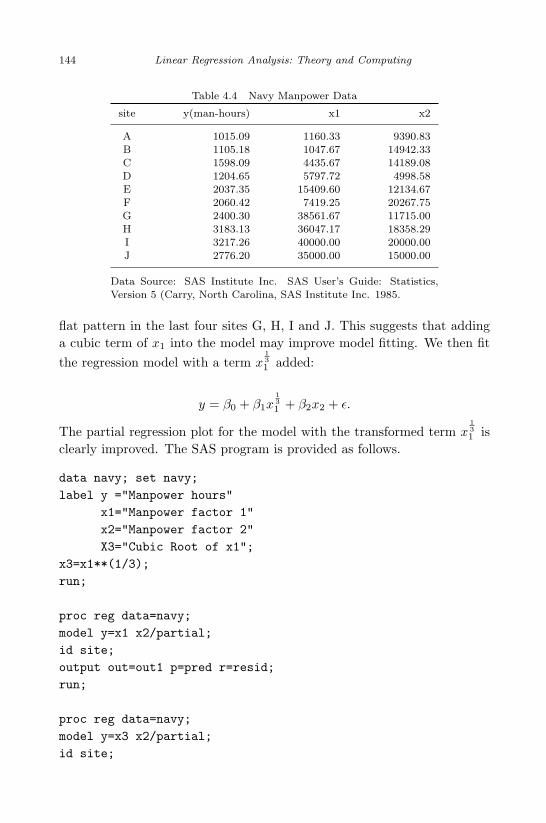
April 29, 2009 11:50 World Scientific Book - 9in x 6in Regression˙master
144 Linear Regression Analysis: Theory and Computing
Table 4.4 Navy Manpower Data
site y(man-hours) x1 x2
A 1015.09 1160.33 9390.83B 1105.18 1047.67 14942.33C 1598.09 4435.67 14189.08D 1204.65 5797.72 4998.58E 2037.35 15409.60 12134.67F 2060.42 7419.25 20267.75G 2400.30 38561.67 11715.00H 3183.13 36047.17 18358.29I 3217.26 40000.00 20000.00J 2776.20 35000.00 15000.00
Data Source: SAS Institute Inc. SAS User’s Guide: Statistics,Version 5 (Carry, North Carolina, SAS Institute Inc. 1985.
flat pattern in the last four sites G, H, I and J. This suggests that addinga cubic term of x1 into the model may improve model fitting. We then fitthe regression model with a term x
131 added:
y = β0 + β1x131 + β2x2 + ε.
The partial regression plot for the model with the transformed term x131 is
clearly improved. The SAS program is provided as follows.
data navy; set navy;
label y ="Manpower hours"
x1="Manpower factor 1"
x2="Manpower factor 2"
X3="Cubic Root of x1";
x3=x1**(1/3);
run;
proc reg data=navy;
model y=x1 x2/partial;
id site;
output out=out1 p=pred r=resid;
run;
proc reg data=navy;
model y=x3 x2/partial;
id site;
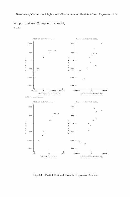
April 29, 2009 11:50 World Scientific Book - 9in x 6in Regression˙master
Detection of Outliers and Influential Observations in Multiple Linear Regression 145
output out=out2 p=pred r=resid;
run;
Fig. 4.1 Partial Residual Plots for Regression Models
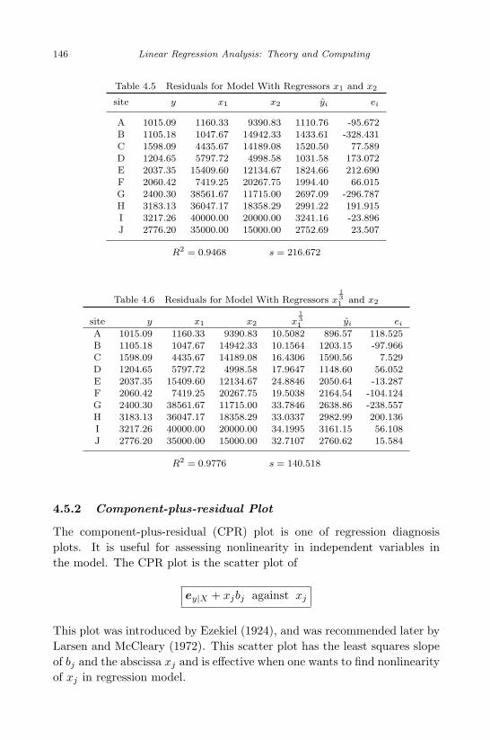
April 29, 2009 11:50 World Scientific Book - 9in x 6in Regression˙master
146 Linear Regression Analysis: Theory and Computing
Table 4.5 Residuals for Model With Regressors x1 and x2
site y x1 x2 yi ei
A 1015.09 1160.33 9390.83 1110.76 -95.672B 1105.18 1047.67 14942.33 1433.61 -328.431C 1598.09 4435.67 14189.08 1520.50 77.589D 1204.65 5797.72 4998.58 1031.58 173.072E 2037.35 15409.60 12134.67 1824.66 212.690F 2060.42 7419.25 20267.75 1994.40 66.015G 2400.30 38561.67 11715.00 2697.09 -296.787H 3183.13 36047.17 18358.29 2991.22 191.915I 3217.26 40000.00 20000.00 3241.16 -23.896J 2776.20 35000.00 15000.00 2752.69 23.507
R2 = 0.9468 s = 216.672
Table 4.6 Residuals for Model With Regressors x131 and x2
site y x1 x2 x131 yi ei
A 1015.09 1160.33 9390.83 10.5082 896.57 118.525B 1105.18 1047.67 14942.33 10.1564 1203.15 -97.966C 1598.09 4435.67 14189.08 16.4306 1590.56 7.529D 1204.65 5797.72 4998.58 17.9647 1148.60 56.052E 2037.35 15409.60 12134.67 24.8846 2050.64 -13.287F 2060.42 7419.25 20267.75 19.5038 2164.54 -104.124G 2400.30 38561.67 11715.00 33.7846 2638.86 -238.557H 3183.13 36047.17 18358.29 33.0337 2982.99 200.136I 3217.26 40000.00 20000.00 34.1995 3161.15 56.108J 2776.20 35000.00 15000.00 32.7107 2760.62 15.584
R2 = 0.9776 s = 140.518
4.5.2 Component-plus-residual Plot
The component-plus-residual (CPR) plot is one of regression diagnosisplots. It is useful for assessing nonlinearity in independent variables inthe model. The CPR plot is the scatter plot of
ey|X + xjbj against xj
This plot was introduced by Ezekiel (1924), and was recommended later byLarsen and McCleary (1972). This scatter plot has the least squares slopeof bj and the abscissa xj and is effective when one wants to find nonlinearityof xj in regression model.
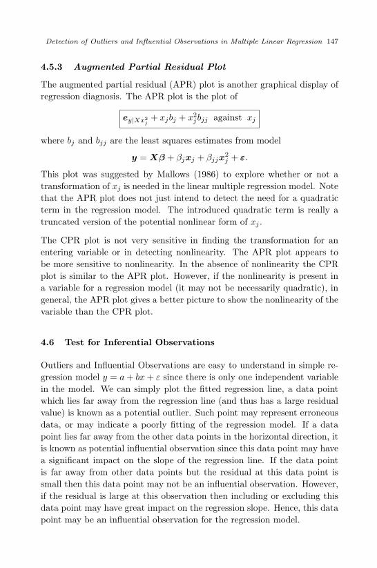
April 29, 2009 11:50 World Scientific Book - 9in x 6in Regression˙master
Detection of Outliers and Influential Observations in Multiple Linear Regression 147
4.5.3 Augmented Partial Residual Plot
The augmented partial residual (APR) plot is another graphical display ofregression diagnosis. The APR plot is the plot of
ey|Xx2j+ xjbj + x2
jbjj against xj
where bj and bjj are the least squares estimates from model
y = Xβ + βjxj + βjjx2j + ε.
This plot was suggested by Mallows (1986) to explore whether or not atransformation of xj is needed in the linear multiple regression model. Notethat the APR plot does not just intend to detect the need for a quadraticterm in the regression model. The introduced quadratic term is really atruncated version of the potential nonlinear form of xj .
The CPR plot is not very sensitive in finding the transformation for anentering variable or in detecting nonlinearity. The APR plot appears tobe more sensitive to nonlinearity. In the absence of nonlinearity the CPRplot is similar to the APR plot. However, if the nonlinearity is present ina variable for a regression model (it may not be necessarily quadratic), ingeneral, the APR plot gives a better picture to show the nonlinearity of thevariable than the CPR plot.
4.6 Test for Inferential Observations
Outliers and Influential Observations are easy to understand in simple re-gression model y = a + bx + ε since there is only one independent variablein the model. We can simply plot the fitted regression line, a data pointwhich lies far away from the regression line (and thus has a large residualvalue) is known as a potential outlier. Such point may represent erroneousdata, or may indicate a poorly fitting of the regression model. If a datapoint lies far away from the other data points in the horizontal direction, itis known as potential influential observation since this data point may havea significant impact on the slope of the regression line. If the data pointis far away from other data points but the residual at this data point issmall then this data point may not be an influential observation. However,if the residual is large at this observation then including or excluding thisdata point may have great impact on the regression slope. Hence, this datapoint may be an influential observation for the regression model.

April 29, 2009 11:50 World Scientific Book - 9in x 6in Regression˙master
148 Linear Regression Analysis: Theory and Computing
The outlier detection for linear regression analysis is to find observationswith larger residuals which are larger than it would actually be produced bychance. i.e., the possible error in y-direction. A data analyst may also wantto identify the extent whether or not these observations influence predictedvalues, estimators of regression coefficients, and performance criteria of aregression model. This is the detection of inferential observations.
Source of influential observation to the regression model depends on thelocation of the observation in either y-direction or x-direction. If a datapoint is far away from the rest of the data points in x-direction this datapoint may be an influential observation since it may affect the slope of thesimple regression line. If a data point is far away from the rest of the datapoints in y-direction then it may not be an influential observation to theregression slope. We now briefly discuss the quantities that could affect theregression model in various ways.
(1) HAT diagonal elements: A data point with a large HAT diagonalelement may or may not be an influential observation to the regressioncoefficients, but it could be an outlier to affect the variance of theestimate of regression coefficients. The HAT diagonal element hii canbe used to detect a possible outlier if
hii = x′i(X
′X)−1xi > 2p/n (4.19)
where n is the total number of observations and p is the number ofindependent variables in the regression model.
(2) R-student residual: Any R-student residual deviates from zero by 2times of the estimated standard error could be a potential outlier.
(3) DFITTS : The DFITTS is defined as the difference between the stan-dardized fitted values with and without the ith observation xi:
DFITTSi =yi − yi,−i
s−i
√hii
(4.20)
It can be shown that
DFITTSi = R-studenti
[ hii
1− hii
]1/2
(4.21)
It can be seen from (4.21) that a larger value of R-studenti or a near-one value of hii may cause the ith observation to be a potential outlier.
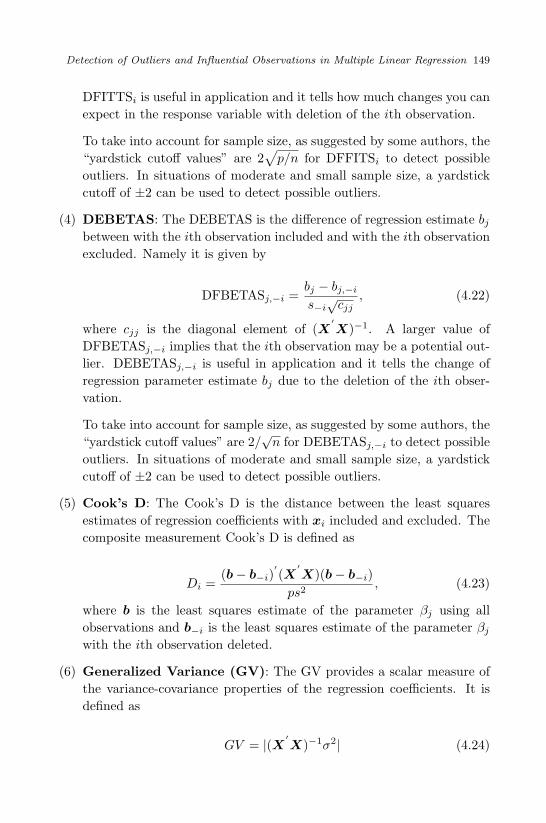
April 29, 2009 11:50 World Scientific Book - 9in x 6in Regression˙master
Detection of Outliers and Influential Observations in Multiple Linear Regression 149
DFITTSi is useful in application and it tells how much changes you canexpect in the response variable with deletion of the ith observation.
To take into account for sample size, as suggested by some authors, the“yardstick cutoff values” are 2
√p/n for DFFITSi to detect possible
outliers. In situations of moderate and small sample size, a yardstickcutoff of ±2 can be used to detect possible outliers.
(4) DEBETAS: The DEBETAS is the difference of regression estimate bj
between with the ith observation included and with the ith observationexcluded. Namely it is given by
DFBETASj,−i =bj − bj,−i
s−i√
cjj, (4.22)
where cjj is the diagonal element of (X′X)−1. A larger value of
DFBETASj,−i implies that the ith observation may be a potential out-lier. DEBETASj,−i is useful in application and it tells the change ofregression parameter estimate bj due to the deletion of the ith obser-vation.
To take into account for sample size, as suggested by some authors, the“yardstick cutoff values” are 2/
√n for DEBETASj,−i to detect possible
outliers. In situations of moderate and small sample size, a yardstickcutoff of ±2 can be used to detect possible outliers.
(5) Cook’s D: The Cook’s D is the distance between the least squaresestimates of regression coefficients with xi included and excluded. Thecomposite measurement Cook’s D is defined as
Di =(b− b−i)
′(X
′X)(b− b−i)
ps2, (4.23)
where b is the least squares estimate of the parameter βj using allobservations and b−i is the least squares estimate of the parameter βj
with the ith observation deleted.
(6) Generalized Variance (GV): The GV provides a scalar measure ofthe variance-covariance properties of the regression coefficients. It isdefined as
GV = |(X ′X)−1σ2| (4.24)

April 29, 2009 11:50 World Scientific Book - 9in x 6in Regression˙master
150 Linear Regression Analysis: Theory and Computing
(7) Covariance Ratio (COVRATIO): The covariance ratio is the ratioof GVs with xi included and excluded. It is defined as
(COVARATIO)i =|(X ′
−iX−i)−1s2−i|
|(X ′X)−1s2| (4.25)
It can be shown that
(COVARATIO)i =(s2−i)
2p
s2p
( 11− hii
)(4.26)
A rough “yardstick cutoff value” for the COVARATIO is suggested byBelsley, Kuh and Welsch (1980). The ith observation may be identifiedas a possible outlier if
(COVARATIO)i > 1 + (3p/n) (4.27)
or
(COVARATIO)i < 1− (3p/n) (4.28)
where p is the number of parameters in regression model and n is thetotal number of observations.
There are much overlap in the information provided by the regression di-agnosis. For example, if the Cook’s D produces an unusually high result,then at least we can expect that one of DEBETASj,i, or one of DIFFITSi
will provide strong result as well. So, information provided by regressiondiagnosis may overlap. Usually, an experienced analyst would briefly lookat the HAT diagnosis and R-student residuals to explore possible outliers.As always, it should be very cautious to remove outliers. Sometimes addingone or more mean shift variables may be a good approach to take.
4.7 Example
In this section we give an illustrative example to calculate residuals, PRESSresiduals, and PRESS statistic for several selected regression models usingthe SAS. The values of the PRESS statistic for different regression modelsare computed and compared in order to select a better regression model.
The following example is based on the Sales of Asphalt Roofing ShingleData (see Table 4.7). The variables in the data set are district code, number
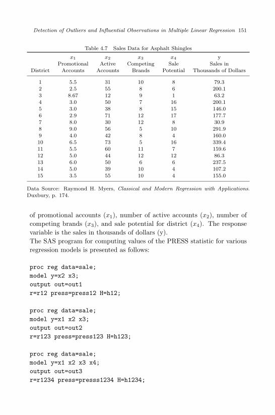
April 29, 2009 11:50 World Scientific Book - 9in x 6in Regression˙master
Detection of Outliers and Influential Observations in Multiple Linear Regression 151
Table 4.7 Sales Data for Asphalt Shingles
x1 x2 x3 x4 yPromotional Active Competing Sale Sales in
District Accounts Accounts Brands Potential Thousands of Dollars
1 5.5 31 10 8 79.32 2.5 55 8 6 200.13 8.67 12 9 1 63.24 3.0 50 7 16 200.15 3.0 38 8 15 146.06 2.9 71 12 17 177.77 8.0 30 12 8 30.98 9.0 56 5 10 291.99 4.0 42 8 4 160.010 6.5 73 5 16 339.411 5.5 60 11 7 159.612 5.0 44 12 12 86.313 6.0 50 6 6 237.514 5.0 39 10 4 107.215 3.5 55 10 4 155.0
Data Source: Raymond H. Myers, Classical and Modern Regression with Applications.Duxbury, p. 174.
of promotional accounts (x1), number of active accounts (x2), number ofcompeting brands (x3), and sale potential for district (x4). The responsevariable is the sales in thousands of dollars (y).The SAS program for computing values of the PRESS statistic for variousregression models is presented as follows:
proc reg data=sale;
model y=x2 x3;
output out=out1
r=r12 press=press12 H=h12;
proc reg data=sale;
model y=x1 x2 x3;
output out=out2
r=r123 press=press123 H=h123;
proc reg data=sale;
model y=x1 x2 x3 x4;
output out=out3
r=r1234 press=presss1234 H=h1234;
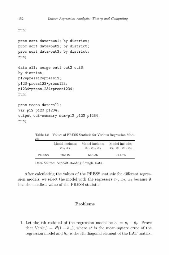
April 29, 2009 11:50 World Scientific Book - 9in x 6in Regression˙master
152 Linear Regression Analysis: Theory and Computing
run;
proc sort data=out1; by district;
proc sort data=out2; by district;
proc sort data=out3; by district;
run;
data all; merge out1 out2 out3;
by district;
p12=press12*press12;
p123=press123*press123;
p1234=press1234*press1234;
run;
proc means data=all;
var p12 p123 p1234;
output out=summary sum=p12 p123 p1234;
run;
Table 4.8 Values of PRESS Statistic for Various Regression Mod-els
Model includes Model includes Model includesx2, x3 x1, x2, x3 x1, x2, x3, x4
PRESS 782.19 643.36 741.76
Data Source: Asphalt Roofing Shingle Data
After calculating the values of the PRESS statistic for different regres-sion models, we select the model with the regressors x1, x2, x3 because ithas the smallest value of the PRESS statistic.
Problems
1. Let the ith residual of the regression model be ei = yi − yi. Provethat Var(ei) = s2(1 − hii), where s2 is the mean square error of theregression model and hii is the ith diagonal element of the HAT matrix.
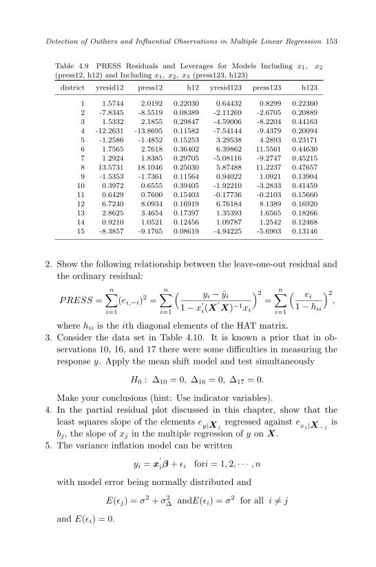
April 29, 2009 11:50 World Scientific Book - 9in x 6in Regression˙master
Detection of Outliers and Influential Observations in Multiple Linear Regression 153
Table 4.9 PRESS Residuals and Leverages for Models Including x1, x2
(press12, h12) and Including x1, x2, x3 (press123, h123)
district yresid12 press12 h12 yresid123 press123 h123
1 1.5744 2.0192 0.22030 0.64432 0.8299 0.223602 -7.8345 -8.5519 0.08389 -2.11269 -2.6705 0.208893 1.5332 2.1855 0.29847 -4.59006 -8.2204 0.441634 -12.2631 -13.8695 0.11582 -7.54144 -9.4379 0.200945 -1.2586 -1.4852 0.15253 3.29538 4.2893 0.231716 1.7565 2.7618 0.36402 6.39862 11.5561 0.446307 1.2924 1.8385 0.29705 -5.08116 -9.2747 0.452158 13.5731 18.1046 0.25030 5.87488 11.2237 0.476579 -1.5353 -1.7361 0.11564 0.94022 1.0921 0.13904
10 0.3972 0.6555 0.39405 -1.92210 -3.2833 0.4145911 0.6429 0.7600 0.15403 -0.17736 -0.2103 0.1566012 6.7240 8.0934 0.16919 6.76184 8.1389 0.1692013 2.8625 3.4654 0.17397 1.35393 1.6565 0.1826614 0.9210 1.0521 0.12456 1.09787 1.2542 0.1246815 -8.3857 -9.1765 0.08619 -4.94225 -5.6903 0.13146
2. Show the following relationship between the leave-one-out residual andthe ordinary residual:
PRESS =n∑
i=1
(ei,−i)2 =n∑
i=1
( yi − yi
1− x′i(X
′X)−1xi
)2
=n∑
i=1
( ei
1− hii
)2
,
where hii is the ith diagonal elements of the HAT matrix.3. Consider the data set in Table 4.10. It is known a prior that in ob-
servations 10, 16, and 17 there were some difficulties in measuring theresponse y. Apply the mean shift model and test simultaneously
H0 : ∆10 = 0, ∆16 = 0, ∆17 = 0.
Make your conclusions (hint: Use indicator variables).4. In the partial residual plot discussed in this chapter, show that the
least squares slope of the elements ey|Xjregressed against exj |X−j
isbj , the slope of xj in the multiple regression of y on X.
5. The variance inflation model can be written
yi = x′iβ + εi fori = 1, 2, · · · , n
with model error being normally distributed and
E(εj) = σ2 + σ2∆ andE(εi) = σ2 for all i 6= j
and E(εi) = 0.

April 29, 2009 11:50 World Scientific Book - 9in x 6in Regression˙master
154 Linear Regression Analysis: Theory and Computing
Table 4.10 Data Set for Multiple Mean Shift Outliers
Observation x1 x2 x3 y
1 12.980 0.317 9.998 57.7022 14.295 2.028 6.776 59.2963 15.531 5.305 2.947 56.1664 15.133 4.738 4.201 55.7675 15.342 7.038 2.053 51.7226 17.149 5.982 -0.055 60.4667 15.462 2.737 4.657 50.7158 12.801 10.663 3.408 37.4419 13.172 2.039 8.738 55.27010 16.125 2.271 2.101 59.28911 14.340 4.077 5.545 54.02712 12.923 2.643 9.331 53.19913 14.231 10.401 1.041 41.89614 15.222 1.22 6.149 63.26415 15.74 10.612 -1.691 45.79816 14.958 4.815 4.111 58.69917 14.125 3.153 8.453 50.08618 16.391 9.698 -1.714 48.89019 16.452 3.912 2.145 62.21320 13.535 7.625 3.851 45.62521 14.199 4.474 5.112 53.92322 16.565 8.546 8.974 56.74123 13.322 8.598 4.011 43.14524 15.945 8.290 -0.248 50.70625 14.123 0.578 -0.543 56.817
To identify variance inflation outlier it is needed to test the hypothesisH0 : σ2
∆ = 0 and the corresponding test statistic is the R-student statis-tic. Thus, the R-student statistic is appropriate for testing regressionoutlier no matter which type of outlier exists.
(a). Show that the (R−student)j has the t-distribution under H0 : σ2∆ =
0.(b). Find the distribution of (R− student)2j under H0 : σ2
∆ 6= 0.
6. The following data in Table 4.11 was collected from a study of the effectof stream characteristics on fish biomass. The regressor variables are
x1: Average depth of 50 cellsx2: Area of stream cover (i.e., undercut banks, logs, boulders, etc.)x3: Percent of canopy cover (average of 12)x4: Area ≥ 25cm in depth
The response variable is y, the fish biomass. The data set is as follows:

April 29, 2009 11:50 World Scientific Book - 9in x 6in Regression˙master
Detection of Outliers and Influential Observations in Multiple Linear Regression 155
Table 4.11 Fish Biomass Data
Observation y x1 x2 x3 x4
1 100 14.3 15.0 12.2 48.02 388 19.1 29.4 26.0 152.23 755 54.6 58.0 24.2 469.74 1288 28.8 42.6 26.1 485.95 230 16.1 15.9 31.6 87.66 0.0 10.0 56.4 23.3 6.97 551 28.5 95.1 13.0 192.98 345 13.8 60.6 7.5 105.89 0.0 10.7 35.2 40.3 0.010 348 25.9 52.0 40.3 116.6
Data Source: Raymond H. Myers: Classical and Mod-ern Regression With Application, p. 201.
(a). Compute s2, Cp, PRESS residuals, and PRESS statistic for themodel y = β0 + β1x1 + β2x2 + β3x3 + β4x4 + ε.
(b). Compute s2, Cp, PRESS residuals, and PRESS statistic for themodel y = β0 + β1x1 + β2x3 + β3x4 + ε.
(c). Compare the regression models from parts (a) and (b) and commentson the prediction of fish biomass.

April 29, 2009 11:50 World Scientific Book - 9in x 6in Regression˙master
This page intentionally left blankThis page intentionally left blank

April 29, 2009 11:50 World Scientific Book - 9in x 6in Regression˙master
Chapter 5
Model Selection
In previous chapters, we have proceeded as if predictors included in themodel, as well as their functional forms (i.e., linear), are known. This iscertainly not the case in reality. Practically, model misspecification occursin various ways. In particular, the proposed model may underfit or overfitthe data, which respectively correspond to situations where we mistak-enly exclude important predictors or include unnecessary predictors. Thus,there involves an issue of variable selection. Furthermore, the simple yetnaive linear functions might be neither adequate nor proper for some pre-dictors. One needs to evaluate the adequacy of linearity for predictors, andif inadequacy identified, seek appropriate functional forms that fit better.
In this chapter, we mainly deal with variable selection, while deferring thelatter issues, linearity assessment and functional form detection, to modeldiagnostics. To gain motivation of and insight into variable selection, wefirst take a look at the adverse effects on model inference that overfitting orunderfitting may cause. Then we discuss two commonly used methods forvariable selection. The first is the method of all possible regressions, whichis most suitable for situations where total number of predictors, p, is smallor moderate. The second type is stepwise algorithmic procedures. Thereare many other concerns that warrant caution and care and new advancesnewly developed in the domain of model selection. We will discuss someimportant ones at the end of the chapter.
5.1 Effect of Underfitting and Overfitting
Consider the linear model y = Xβ+ε, where X is n×(k+1) of full columnrank (k+1) and ε ∼ MVN0, σ2 ·I. To facilitate a setting for underfitting
157
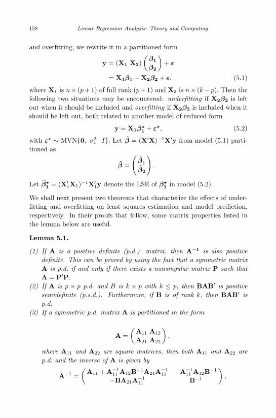
May 7, 2009 10:22 World Scientific Book - 9in x 6in Regression˙master
158 Linear Regression Analysis: Theory and Computing
and overfitting, we rewrite it in a partitioned form
y = (X1 X2)(
β1
β2
)+ ε
= X1β1 + X2β2 + ε, (5.1)
where X1 is n× (p + 1) of full rank (p + 1) and X2 is n× (k− p). Then thefollowing two situations may be encountered: underfitting if X2β2 is leftout when it should be included and overfitting if X2β2 is included when itshould be left out, both related to another model of reduced form
y = X1β1 + ε, (5.2)
with ε ∼ MVN0, σ2 · I. Let β = (X′X)−1X′y from model (5.1) parti-
tioned as
β =
(β1
β2
).
Let β1 = (X′
1X1)−1X′1y denote the LSE of β
1 in model (5.2).
We shall next present two theorems that characterize the effects of under-fitting and overfitting on least squares estimation and model prediction,respectively. In their proofs that follow, some matrix properties listed inthe lemma below are useful.
Lemma 5.1.
(1) If A is a positive definite (p.d.) matrix, then A−1 is also positivedefinite. This can be proved by using the fact that a symmetric matrixA is p.d. if and only if there exists a nonsingular matrix P such thatA = P′P.
(2) If A is p × p p.d. and B is k × p with k ≤ p, then BAB′ is positivesemidefinite (p.s.d.). Furthermore, if B is of rank k, then BAB′ isp.d.
(3) If a symmetric p.d. matrix A is partitioned in the form
A =(
A11 A12
A21 A22
),
where A11 and A22 are square matrices, then both A11 and A22 arep.d. and the inverse of A is given by
A−1 =(
A11 + A−111 A12B−1A21A−1
11 −A−111 A12B−1
−BA21A−111 B−1
),

April 29, 2009 11:50 World Scientific Book - 9in x 6in Regression˙master
Model Selection 159
with B = A22−A21A−111 A12. Besides, one can verify by straightforward
algebra that
(x′1 x′2 ) A−1
(x1
x2
)= x′1A
−111 x1 + b′B−1b, (5.3)
where b = x2 −A21A−111 x1.
Theorem 5.1. Suppose that Model y = X1β1 + X2β2 + ε is the trueunderlying model, but we actually fit model y = X1β
?1 + ε?, which is thus
an underfitted model. Then:
(i) E(β?1) = β1 + Aβ2, where A = (X′
1X1)−1X′1X2.
(ii) Cov(β?1) = σ2(X′
1X1)−1 and
Cov(β1) = σ2 · (X′1X1)−1 + AB−1A′ ,
where B = X′2X2 −X′
2X1(X′1X1)−1X′
1X2. We have
Cov(β1)− Cov(β?1) ≥ 0 i.e. positive semi-definite.
(iii) Let V1 denote the column space of X1 and
PV⊥1 = I−PV1 = I−X1(X′1X1)−1X′
1
be the projection matric of subspace V⊥1 . Then an estimator of σ2
σ2 =‖ PV⊥1 y ‖2n− p− 1
has the expected value of
E(σ2) = σ2 +‖ PV⊥1 (X′
2β2) ‖2n− p− 1
.
(iv) Given x0 =(
x01
x02
), let y? = x′01β
?1 denote the estimate based on the
working model and y0 = x′0β =(
y01
y02
)denote the estimate based on
the true model. Then it can be found that
E(y?) = x′01 (β1 + Aβ2)
and
Var(y?) = σ2 · x′01(X′1X1)−1x01 ≤ min Var(y01),Var(y0) ,
where Var(y01) = Var(x′01β1).
April 29, 2009 11:50 World Scientific Book - 9in x 6in Regression˙master
160 Linear Regression Analysis: Theory and Computing
Proof.
(i) Consider
E(β?1) = E(X′
1X1)−1X′1y = (X′
1X1)−1X′1E(y)
= (X′1X1)−1X′
1(X1β1 + X2β2)
= β1 + (X′1X1)−1X′
1X2β2
(ii) First
Cov(β?) = cov(X′1X1)−1X′
1y= (X′
1X1)−1X′1(σ2I)X1(X′
1X1)−1
= σ2(X′1X1)−1
Next, to find Cov(β1), consider
Cov(β) = Cov
(β1
β2
)= σ2 · (X′X)−1 = σ2
(X′
1X1 X′1X2
X′2X1 X′
2X2
)−1
= σ2
(G11 G12
G21 G22
),
where Gij is the corresponding block of the partitioned inverse matrix(X′X)−1. It can be found that
G11 = (X′1X1)−1 + AB−1A′ and G22 = B−1
Hence, Cov(β1) − Cov(β?1) = σ2AB−1A′. Now (X′X)−1 is p.d., so
is G22 = B−1. Hence, matrix AB−1A′ is p.s.d. This implies thatVar(βj) ≥ Var(β?
j ).(iii) The sum of squared error, SSE1, associated with model y = X1β
?1+ε?
is
SSE1 = ‖ y −X1β? ‖2=‖ y − PV1y ‖2
= ‖ PV⊥1 y ‖2= y′PV⊥1 y.
We have
E(SSE1) = E(y′PV⊥1 y) = trPV⊥1 σ2I+ β′X′PV⊥1 Xβ
= (n− p− 1)σ2+ ‖ PV⊥1 (X1β1 + X2β2) ‖2
= (n− p− 1)σ2+ ‖ PV⊥1 (X2β2) ‖2, (5.4)
since PV⊥1 (X1β1) = 0. Therefore,
E(σ2) =E(SSE1)n− p− 1
= σ2 +‖ PV⊥1 (X′
2β2) ‖2n− p− 1
,
which is larger than or equal to σ2.

April 29, 2009 11:50 World Scientific Book - 9in x 6in Regression˙master
Model Selection 161
(iv) First,
E(y?0) = E(x′01β
?
1 = x′01(β1 + Aβ2) 6= x′01β1
= x′0β − (x02 −A′x01)′β2 6= x′0β.
Next, it can be found that
Var(y?0) = x′01Cov(β?
1x01) = σ2x′01(X′X)−1x01.
On the other hand,
Var(y01) = Var(x′01β1) = x′01Cov(β1)x01
= σ2 · x′01(X′
1X1)−1 + AB−1A′x01
≥ Var(y?0).
Also,
Var(x′0β) = σ2 · x′0(X′X)−1x0
= σ2 · x′01(X′1X1)−1x01 + σ2 · b′B−1b by equation (5.3),
≥ σ2 · x′01(X′1X1)−1x01 = Var(y?
0), as B−1 is p.d.,
where b = x02 −A′x01. ¤
Theorem 5.1 indicates that underfitting would result in biased estimationand prediction, while leading to deflated variance. Subsequently, we con-sider the overfitting scenario.
Theorem 5.2. Suppose that model y = X1β?1 + ε? is the true underlying
model, but we actually fit model y = X1β1 + X2β2 + ε, an overfitted one.Then
(i) E(β) =(
β?1
0
).
(ii) Cov(β) = σ2? · (X′X)−1 and Cov(β1) = σ2
? ·(X′
1X1)−1 + AB−1A′ .
Again, compared to Cov(β?) = σ2
? · (X′1X1)−1, we have Cov(β1) −
Cov(β?1) ≥ 0, i.e. positive semi-definite.
(iii) An estimator of σ2?,
σ2? =
‖ PV⊥y ‖2n− k − 1
has the expected value of σ2?.

April 29, 2009 11:50 World Scientific Book - 9in x 6in Regression˙master
162 Linear Regression Analysis: Theory and Computing
(iv) Given x0 =(
x01
x02
), let y0 = x′0β =
(y01
y02
)denote the estimate based
on the working model and y? = x′01β?1 denote the estimate based on
the true model. Then it can be found that E(y) = x′01β?1 and Var(y) =
σ2? · x′0(X′X)−1x0 ≥ Var(y?).
Proof. We will prove (i) and (iii) only, leaving the rest for exercise.
(i) Consider
E(β) = E(X′X)−1X′y = (X′X)−1X′X1β?1
= (X′X)−1X′ (X1 X1
) (β?
1
0
)
= (X′X)−1X′X(
β?1
0
)=
(β?
1
0
)
(iii) Consider the SSE associated with Model (5.1),
E(SSE) = E(y′PV⊥y) = trPV⊥σ2?I+ β?
1′X′
1PV⊥X1β?1
= (n− k − 1)σ2?,
since PV⊥(X1β?1) = 0. Thus, E(σ2
?) = E SSE/(n− k − 1) = σ2?.
¤
Theorem 5.2 implies that overfitting would yield unbiased estimation andprediction, however result in inflated variances.
Example (A Simulation Study) In some situations such as predictivedata mining, prediction accuracy is the ultimate yardstick to judge themodel performance. In order to see how overfitting or underfitting affectsthe generalization ability of a model to new observations, one may studythe sum of squared prediction error (SSPE) within the similar theoreticalframework as in Theorems 5.1 and 5.2. Alternatively, empirical evaluationcan be made via simulation studies. Here, we illustrate the latter approachusing a simple example. The data are generated from the following model
y = β0 + β1x1 + · · ·+ β10x10 + ε,
with xj ∼ uniform(0, 1) and ε ∼ N(0, 1) independently. Each data setalso includes 20 additional predictors, also from uniform(0,1), which aretotally unrelated to the response. In each simulation run, we generatedtwo data sets: a set containing 1000 observations and another independent
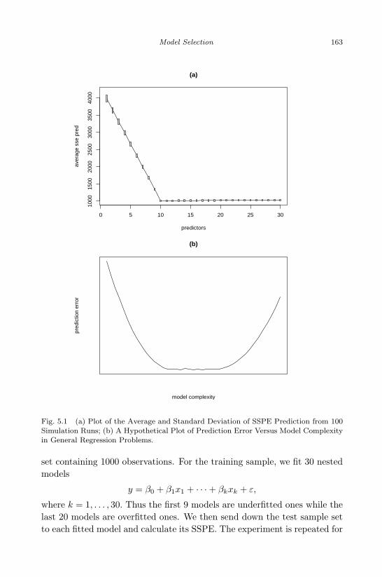
April 29, 2009 11:50 World Scientific Book - 9in x 6in Regression˙master
Model Selection 163
0 5 10 15 20 25 30
1000
1500
2000
2500
3000
3500
4000
(a)
predictors
aver
age
sse
pred
(b)
model complexity
pred
ictio
n er
ror
Fig. 5.1 (a) Plot of the Average and Standard Deviation of SSPE Prediction from 100Simulation Runs; (b) A Hypothetical Plot of Prediction Error Versus Model Complexityin General Regression Problems.
set containing 1000 observations. For the training sample, we fit 30 nestedmodels
y = β0 + β1x1 + · · ·+ βkxk + ε,
where k = 1, . . . , 30. Thus the first 9 models are underfitted ones while thelast 20 models are overfitted ones. We then send down the test sample setto each fitted model and calculate its SSPE. The experiment is repeated for

May 7, 2009 10:22 World Scientific Book - 9in x 6in Regression˙master
164 Linear Regression Analysis: Theory and Computing
100 simulation runs and we integrated the results by computing the averageand standard deviation (sd) of SSPE values for each of the 30 models.
Figure 5.1 (a) gives a plot of the results. The line shows the averageSSPE and the hight of the vertical bar at each point corresponds to the sdof the SSPE values for each model. It can be seen that both the averageof SSPE reaches the minimum when the true model is fit. However, theaveraged SSPE is inflated much more in the underfitting cases than in theoverfitting ones. A similar observation can be drawn for the sd of SSPE.The pattern shown here about the prediction error is generally true inmany regression problems. When the model complexity increases startingfrom the null model, the prediction error drops gradually to its bottom andthen slowly increases after a flat valley, as shown in a hypothetical plot inFig. 5.1 (b). The specific shape of the curve and length of the flat valleywould vary depending on types of the regression methods being used, thesignal-to-noise ratio in the data, and other factors.
In summary, both underfitting and overfitting cause concerns. Althougha simplified scenario for model mis-specification has been employed tomake inference, we, again, see that underfitting leads to biased estima-tion and overfitting leads to increased variances, which is the well-knownbias-variance tradeoff principle. The task of variable selection is to seek anappropriate balance between this bias-variance tradeoff.
The bias-variance tradeoff can also be viewed via the concept of meansquare error (MSE). In statistics, MSE is a widely used criterion for mea-suring the quality of estimation. Consider a typical problem of estimatingparameter θ, which may correspond to the true effect or sloe of a predictor,or prediction for a new observation. Let θ be an estimator of θ. The MSEof θ is defined as
MSE(θ) = E(θ − θ)2. (5.5)MSE provides a way, by applying the squared error loss, to quantify theamount by which an estimator differs from the true value of the parameterbeing estimated. Note that MSE is an expectation, a real number, not arandom variable. It may be a function of the unknown parameter θ, but itdoes not involve any random quantity. It can be easily verified that
MSE(θ) = E[
θ − E(θ)
+E(θ)− θ
]2= E
θ − E(θ)
2
+E(θ)− θ
2
= Var(θ) + bias2(θ). (5.6)
April 29, 2009 11:50 World Scientific Book - 9in x 6in Regression˙master
Model Selection 165
Namely, MSE is the the sum of the variance and the squared bias of theestimator θ. An under-fitted model suffers from bias in both estimationof the regression coefficients and the regression prediction while an over-fitted model suffers from inflated variance. It is reasonable to expect thata good balance between variance and bias is achieved by models that yieldsmall MSEs. This idea motivates the derivation of a model selection criteriacalled Mellow’s Cp, as we shall discuss in the next section.
5.2 All Possible Regressions
In the method of all possible regressions (also called all subset regressions),one evaluates all model choices by trying out every possible combination ofpredictors and then compares them via a model selection criterion. Supposethere are k predictors in total. Excluding the null model that has theintercept term only, there are a total of 2k − 1 different combinations. Ifk ≥ 20 for example, which is not uncommon at all in real applications, then2k − 1 ≥ 1, 048, 575 possible distinct combinations need to be considered.It is abundantly clear that this method is feasible only when the numberof predictors in the data set is moderately small.
There have been many criteria proposed in the literature for evaluatingthe performance of competing models. These are often referred to as modelselection criteria. As we have seen in section 5.1, a simple model leads tosmaller variation, yet with biased or inaccurate estimation, while a complexmodel yields unbiased estimation or better goodness-of-fit to the currentdata, yet with inflated variation or imprecise estimation. As we will see,many model selection criteria are intended to balance off between bias andvariation by penalizing the goodness-of-fit of the model with its complexity.
5.2.1 Some Naive Criteria
A natural yet naive criterion for model evaluation is the sum of squareerrors,
SSE =∑
(yi − yi)2,
which yields an overall distance between observed responses and their pre-dicted values. A good model is expected to have relatively small SSE. How-ever, it is known that for nested models, a smaller SSE is always associatedwith a more complex model. As a result, the full model that includes all
April 29, 2009 11:50 World Scientific Book - 9in x 6in Regression˙master
166 Linear Regression Analysis: Theory and Computing
predictors would have the smallest SSE. Therefore, SSE alone is not a goodmodel selection criterion for direct use, because it measures goodness-of-fitonly and fails to take model complexity into consideration.
Similar conclusion applies to the coefficient of determination,
R2 = 1− SSE
SST,
which is a monotone increasing function of SSE, noting that the sum ofsquare total SST stays invariant with different model choices. Nevertheless,R2 is a very popular goodness-of-fit measure due to its easy interpretation.
With a slight modification on R2, the adjusted R-squared is defined as
R2a = 1− MSE
s2y
,
where s2y is the sample variance of Y . After replacing the sum of squares in
R2 by mean squares, R2a is not necessarily increasing with model complexity
for nested models. However, R2a, as well as MSE, is inadequate as a criterion
for variable selection. Besides, it lacks the easy interpretability of R2 asthe proportion of the total variation in observed responses that can beaccounted for by the regression model. In fact, R2
a turns out to be not veryuseful for practical purposes.
5.2.2 PRESS and GCV
In predictive modeling tasks, candidates models are often evaluated basedon their generalization abilities. If the sample size is large, the commonapproach is to employ an independent test sample. To do so, one partitionsthe whole data L into two parts: the training (or learning) set L1 and thetest set L2. Candidate models are then built or estimated using the trainingset L1 and validated with the test set L2. Models that yield small sum ofsquared prediction errors for L2,
SSPE =∑
i∈L2
(yi − yi)2, (5.7)
are preferable. Note that, in (5.7), yi is the predicted value based on themodel fit obtained from training data, would be preferable.
When an independent test data set is unavailable due to insufficientsample size, one has to get around, either analytically or by efficient samplere-use, in order to facilitate validation. The prediction sum of squares

April 29, 2009 11:50 World Scientific Book - 9in x 6in Regression˙master
Model Selection 167
(PRESS) criterion is of the latter type. Related to the jackknife technique,PRESS is defined as
PRESS =n∑
i=1
yi − yi(−i)
2, (5.8)
where yi(−i) is the predicted value for the ith case based on the regressionmodel that is fitted by excluding the ith case. The jackknife or leave-one-outmechanism utilizes the independence between yi and yi(−i) and facilitates away of mimicking the prediction errors. A small PRESS value is associatedwith a good model in the sense that it yields small prediction errors. Tocompute PRESS, one does not have to fit the regression model repeatedlyby removing each observation at a time. It can be shown that
PRESS =n∑
i=1
(ei
1− hii
)2
, (5.9)
where ei = yi − yi is the ith ordinary residual and hii is the ith leveragedefined as the ith diagonal element of the hat or projection matrix H =X(X′X)−1X′.
PRESS is heavily used in many modern modeling procedures besides linearregression. In scenarios where explicit computation of the components hii’sis difficult, Craven and Wahba (1979) proposed to replace each of hi’s inPRESS/n by their average tr(H)/n = (p + 1)/n, which leads to the well-known generalized cross-validation (GCV) criterion. Nevertheless, it canbe easily shown that in linear regression
GCV =1n·
∑ni=1 e2
i
1− (p + 1)/n2 =n · SSE
n− (p + 1)2 =n
n− (p + 1)·MSE.
(5.10)In Section 7.3.4, the use of PRESS and GCV is further discussed in moregeneral settings.
5.2.3 Mallow’s CP
Subsequently we shall introduce several criteria that are derived analyti-cally. The first one is the Cp criterion proposed by Mellows (1973). TheCp criterion is concerned with the mean squared errors of the fitted values.
Its derivation starts with assuming that the true model that generatesthe data is a massive full linear model involving many predictors, perhapseven those on which we do not collect any information. Let X, of dimension

April 29, 2009 11:50 World Scientific Book - 9in x 6in Regression˙master
168 Linear Regression Analysis: Theory and Computing
n× (k +1), denote the design matrix associated with this full model, whichcan then be stated as
y = Xβ + ε with ε ∼ MVN0, σ2 · I. (5.11)Furthermore, it is assumed that the working model is a sub-model nestedinto the full true model. Let X1, of dimension n×(p+1), denote the designmatrix associated with the working model:
y = X1β?1 + ε? with ε? ∼ MVN0, σ2
? · I. (5.12)Thus, the setting employed here is exactly the same as that in Section 5.1.The working model (5.12) is assumed to underfit the data.
To evaluate a typical working model (5.12), we consider the performanceof its fitted values y = (yi) for i = 1, . . . , n. Let V1 = C(X1) be the columnspace of matrix X1 and H1 = PV1 = X1(Xt
1X1)tXt1 be the projection
matrix of V1. Then the fitted mean vector from the working model (5.12)is
y = H1y, (5.13)which is aimed to estimate or predict the true mean response vectorµ = Xβ. Since model (5.12) provides underfitting, y with E(y) = H1Xβ isbiased for Xβ. For model selection purpose, however, we seek the best pos-sible working model that provides the smallest mean squared error (MSE),recalling that a small MSE balances the bias-variance tradeoff.
The MSE of y, again, can be written as the sum of variance and squaredbias:
MSE(y) = E(y −Xβ)t(y −Xβ)
=
∑
i
E(yi − xtiβ)2
=n∑
i=1
[E(yi)− xtiβ2 + Var(yi)
]
=n∑
i=1
bias2(yi) +n∑
i=1
Var(yi). (5.14)
Denote the bias part in (5.14) as B. Using the results established in Section5.1, it follows that
B =n∑
i=1
bias(yi)2 = E(y)−Xβt E(y)−Xβ
= (H1Xβ −Xβ)t (H1Xβ −Xβ) = βtX(I−H1)Xβ
= (X1β1 + X2β2)t(I−H1)(X1β1 + X2β2)
= (βt2X2)t(I−H1)(βt
2X2), since (I−H1)X1 = PV⊥1 X1 = 0
= E(SSE1)− (n− p− 1)σ2 using (5.4), (5.15)

April 29, 2009 11:50 World Scientific Book - 9in x 6in Regression˙master
Model Selection 169
where SSE1 is the residual sum of squares from fitting the working model(5.12). Denote the variance part in (5.14) as V , which is
V =n∑
i=1
Var(yi) = trace Cov(y)
= trace Cov(H1y) = traceσ2 ·H1
= (p + 1) · σ2. (5.16)
Thus, bringing (5.15) and (5.16) into (5.14) yields that
MSE(y) = B + V = E(SSE1)− σ2 · n− 2(p + 1). (5.17)
The Cp criterion is aimed to provide an estimate of the MSE in (5.17) scaledby σ2, i.e.,
MSE(y)σ2
=E(SSE1)
σ2− n− 2(p + 1).
Thus the Cp criterion is specified as
Cp =SSE1
MSEfull− n− 2(p + 1), (5.18)
where the true error variance σ2 is estimated by MSEfull, the mean squarederror from the full model that includes all predictors.
When there is no or little bias involved in the current working modelso that B ≈ 0 in (5.17), the expected value of Cp is about V/σ2 = (p + 1).Models with substantial bias tend to yield Cp values much greater than(p+1). Therefore, Mellows (1975) suggests that any model with Cp < (p+1)be a candidate. It is, however, worth noting that the performance of Cp
depends heavily on whether MSEfull provides a reliable estimate of thetrue error variance σ2.
5.2.4 AIC, AICC, and BIC
Akaike (1973) derived a criterion from information theories, known as theAkaike information criterion (AIC). The AIC can be viewed as a data-based approximation for the Kullback-Leibler discrepancy function betweena candidate model and the true model. It has the following general form:
AIC = n× log-likelihood + 2× number of parameters.
When applied to Gaussian or normal models, it becomes, up to a constant,
AIC ' n · log(SSE) + 2 p.
April 29, 2009 11:50 World Scientific Book - 9in x 6in Regression˙master
170 Linear Regression Analysis: Theory and Computing
The first part 2 · log(SSE) measures the goodness-of-fit of the model, whichis penalized by model complexity in the second part 2p. The constant 2 inthe penalty term is often referred to as complexity or penalty parameter.The smaller AIC results in the better candidate model.
It is noteworthy that Cp is equivalent to GCV in (5.10) in view ofapproximation 1/(1− x)2 = 1 + 2x (see Problem 5.7), both having similarperformance as AIC. All these three criteria are asymptotically equivalent.
Observing that AIC tends to overfit when the sample size is relatively small,Hurvich and Tsai (1989) proposed a bias-corrected version, called AICC ,which is given by
AICC ' n · log(SSE) +n · (n + p + 1)
n− p− 3.
Within the Bayesian framework, Schwarz (1978) developed another crite-rion, labeled as BIC for Bayesian information criterion (or also SIC forSchwarz information criterion and SBC for Schwarz-Bayesian criterion).The BIC, given as
BIC ' n · log(SSE) + log(n) p,
applies a larger penalty for overfitting. The information-based criteriahave received wide popularity in statistical applications mainly becauseof their easy extension to other regression models. There are many otherinformation-based criteria introduced in the literature.
In large samples, a model selection criterion is said to be asymptoticallyefficient if it is aimed to select the model with minimum mean squarederror, and consistent if it selects the true model with probability one. Nocriterion is both consistent and asymptotically efficient. According to thiscategorization, MSE, R2
a, GCV , Cp, AIC, and AICC are all asymptoti-cally efficient criteria while BIC is a consistent one. Among many otherfactors, the performance of these criteria depends on the available samplesize and the signal-to-noise ratio. Based on the extensive simulation stud-ies, McQuarrie and Tsai (1998) provided some general advice on the use ofvarious model selection criteria, indicating that AIC and Cp work best formoderately-sized sample, AICC provides the most effective selection withsmall samples, while BIC is most suitable for large samples with relativelystrong signals.

April 29, 2009 11:50 World Scientific Book - 9in x 6in Regression˙master
Model Selection 171
5.3 Stepwise Selection
As mentioned earlier, the method of all possible regressions is infeasiblewhen the number of predictors is large. A common alternative in this case isto apply a stepwise algorithm. There are three types of stepwise proceduresavailable: backward elimination, forward addition, and stepwise search. Inthese algorithmic approaches, variables are added into or deleted from themodel in an iterative manner, one at a time. Another important featureof stepwise selection is that competitive models evaluated in a particularstep have the same complexity level. For this reason, measures such asSSE or R2 can be directly used for model comparisons with equivalence toother model selection criteria such as AIC. In order to determine a stoppingrule for the algorithm, a test statistic is often employment instead, which,nevertheless, inevitably raises the multiplicity concern. A natural choice,as implemented in SAS, is the F statistic that evaluates the reduction inType III sum of squares (SS) or the main effect of each individual predictor.In the R implementation stepAIC(), AIC is used instead, in which casethe procedure stops when further modification (i.e., adding or deleting aselected variable) on the model no longer decreases AIC.
5.3.1 Backward Elimination
The backward elimination procedure proceeds as follows. Start with fit-ting the whole model that includes all k predictors. For each predictorXj , compute the F test statistic that compares the whole model with thereduced model that excludes Xj . Identify the least significant predictorX? that corresponds to the largest p-value associated with the F test. Ifthis largest p-value is smaller than a threshold significance level αstay, theprocedure is stopped and this whole model is claimed as the final model.Otherwise, we remove X? from the current model and fit the model thatcontains the remaining k−1 predictors. Next, the least significant predictoris identified and may be removed by examining the F test statistics andtheir p-values. This procedure is repeated till all p-values in the model areless than αstay. The resultant model is then claimed as the final model.
The final model identified by backward elimination is sensitive to the thresh-old αstay. Common choices for αstay are 0.10 and 0.05. The default valuein SAS is 0.10. Backward elimination is the most computationally efficientone among the three stepwise procedures. It takes at most k steps or model
April 29, 2009 11:50 World Scientific Book - 9in x 6in Regression˙master
172 Linear Regression Analysis: Theory and Computing
fittings to arrive at a final model. This property renders it a popular vari-able selection or screening method in situations where the data set containsa large number of predictors. Nevertheless, there is one problem with back-ward elimination. That is, a dropped variable would have no more chanceto re-enter the model. However, a variable that has been excluded in anearlier stage may become significant after dropping other predictors.
5.3.2 Forward Addition
Forward addition is sort of like a reversed procedure of backward elimina-tion. Starting with the null model that has the intercept only, the procedurefits all k simple linear regression models, each with one predictor includedonly. Again, the F test statistic that compares each simple linear modelwith the null is computed, as well as its corresponding p-value. Let X?
denote the most significant predictor, the one associated with the small-est p-value. This very first step amounts to find the predictor that hasthe highest correlation with Y . If this smallest p-value is smaller than athreshold significance level αentry, the procedure is stopped and the nullmodel is claimed as the final model. Otherwise, X? is added into the nullmodel. Subsequently, with X? included, one identifies the next most sig-nificant variable to add. This procedure is repeated till no more variable iseligible to add.
The default value for αentry in SAS is 0.05. Computationally, forwardaddition is slower than backward deletion. It involves at most k +(k−1)+· · ·+ 1 = k(k + 1)/2 model fittings to finally stop. The problem associatedwith forward addition is analogous to the one with backward elimination.Once added, a variable would always stay in the final model. However, avariable that was added in an earlier stage may become insignificant afterincluding other predictors into the model. As a matter of fact, forwardaddition is not very often used in applications.
5.3.3 Stepwise Search
The stepwise search method is intended to avoid the problems with bothbackward elimination and forward addition so that variables already in themodel may be removed due to insignificance and variables excluded maybe added later on when it becomes significant. The procedure itself is moresimilar to the forward addition algorithm. As in forward addition, the mostsignificant variable is added to the model at each step, if its corresponding

May 7, 2009 10:22 World Scientific Book - 9in x 6in Regression˙master
Model Selection 173
F test is significant at the level of αentry. Before the next variable is added,however, the stepwise search method takes an additional look-back step tocheck all variables included in the current model and deletes any variablethat has a p-value greater than αstay. Only after the necessary deletions areaccomplished can the procedure move to the next step of adding anothervariable into the model. The stepwise search continues till every variablein the model is significant at the αstay level and every variables not in themodel is insignificant at the αentry level if added.
Among all three stepwise selection procedures, the stepwise search algo-rithm performs best, although computationally the backward eliminationalgorithm is the fastest one.
One should be very careful with these automatic selection procedures. Sincea largest number of F tests have been conducted, there is a very high prob-ability of making Type I error (including unimportant predictors) and TypeII error (excluding important predictors). As demonstrated via simulationin Cook and Weisberg (1999), the algorithmic stepwise model selectioncan considerably overstate the significance of predictors. The predictorsleft in the final model may appear much more important than they reallyare. Furthermore, there are arguments indicating that, same as other data-adaptive algorithms, results from stepwise procedures are sample-specificand unlikely to replicate. See, e.g., Thompson (2001). This is because asmall change or variation that is specific to one sample may give a predic-tor an advantage over another that it would not have been seen in othersamples, making stepwise selection results unlikely to generalize. Besides,in order to arrive at a successful model fit, one needs consider transforma-tions such as high-order terms and interactions among predictors. Thus itis sometimes advised to use stepwise procedures for variable screening pur-poses only, instead of for final model determination. Furthermore, even ifa ‘best’ model is obtained, there are still model diagnostic issues to follow.Diagnostic results may suggest further modifications of the model. Thus itis also advised to conduct the model building process in an iterative mannerby alternating between model selection and model diagnostics.
5.4 Examples
To illustrate, we first consider an astronomical data set taken from Ex. 4.9in Mendenhall and Sinich (2003).

April 29, 2009 11:50 World Scientific Book - 9in x 6in Regression˙master
174 Linear Regression Analysis: Theory and Computing
Table 5.1 The Quasar Data from Ex. 4.9 in Mendenhall and Sinich (2003)
Line Absolute Rest FrameRedshift Line Flux Luminosity AB1450 Magnitude Equivalent
Quasar (X1) (X2) (X3) (X4) (X5) Width (Y )
1 2.81 -13.48 45.29 19.5 -26.27 1172 3.07 -13.73 45.13 19.65 -26.26 823 3.45 -13.87 45.11 18.93 -27.17 334 3.19 -13.27 45.63 18.59 -27.39 925 3.07 -13.56 45.3 19.59 -26.32 1146 4.15 -13.95 45.2 19.42 -26.97 507 3.26 -13.83 45.08 19.18 -26.83 438 2.81 -13.5 45.27 20.41 -25.36 2599 3.83 -13.66 45.41 18.93 -27.34 5810 3.32 -13.71 45.23 20 -26.04 12611 2.81 -13.5 45.27 18.45 -27.32 4212 4.4 -13.96 45.25 20.55 -25.94 14613 3.45 -13.91 45.07 20.45 -25.65 12414 3.7 -13.85 45.19 19.7 -26.51 7515 3.07 -13.67 45.19 19.54 -26.37 8516 4.34 -13.93 45.27 20.17 -26.29 10917 3 -13.75 45.08 19.3 -26.58 5518 3.88 -14.17 44.92 20.68 -25.61 9119 3.07 -13.92 44.94 20.51 -25.41 11620 4.08 -14.28 44.86 20.7 -25.67 7521 3.62 -13.82 45.2 19.45 -26.73 6322 3.07 -14.08 44.78 19.9 -26.02 4623 2.94 -13.82 44.99 19.49 -26.35 5524 3.2 -14.15 44.75 20.89 -25.09 9925 3.24 -13.74 45.17 19.17 -26.83 53
a Source: Schmidt, M., Schneider, D. P., and Gunn, J. E. (1995) Spectroscopic CCDsurveys for quasars at large redshift. The Astronomical Journal, 110, No. 1, p. 70(Table 1).
Example 5.1 A quasar is a distant celestial object that is at least fourbillion light-years away from earth. The Astronomical Journal (Schmidt,M., Schneider, D. P., and Gunn, J. E., 1995) reported a study of 90 quasarsdetected by a deep space survey. Based on the radiations provided byeach quasar, astronomers were able to measure several of its quantitativecharacteristics, including redshift range (X1), line flux in erg/cm2 (X2), linelunminosity in erg/s (X3), AB1450 magnitude (X4), absolute magnitude(X5), and rest frame equivalent width (Y ). One objective of the study isto model the rest frame equivalent width (Y ) using other characteristics.The data for a sample of 25 large quasars, as given in Table 5.1, are usedin this example.

April 29, 2009 11:50 World Scientific Book - 9in x 6in Regression˙master
Model Selection 175
data quasar;
input obs x1 x2 x3 x4 x5 y;
y = log(y);
cards;
1 2.81 -13.48 45.29 19.50 -26.27 117
2 3.07 -13.73 45.13 19.65 -26.26 82
......
25 3.24 -13.74 45.17 19.17 -26.83 53
;
Table 5.2 All Possible Regression Selection for the Quasar Data.
# of Variables Adjusted Variablesin Model R2 R2 Cp AIC BIC in the Model
1 0.4383 0.4139 63741.50 −48.4771 −52.4740 X5
0.3938 0.3674 68798.74 −46.5690 −50.5661 X4
0.0317 −.0104 109901.7 −34.8618 −38.8600 X3
0.0219 −.0206 111008.5 −34.6114 −38.6096 X2
0.0001 −.0433 113483.1 −34.0603 −38.0585 X1
2 0.9997 0.9997 16.6433 −233.7111 −233.6811 X3 X5
0.9637 0.9604 4100.948 −114.9603 −120.8996 X2 X4
0.8468 0.8328 17377.12 −78.9501 −84.9357 X3 X4
0.7560 0.7339 27674.90 −67.3260 −73.3169 X2 X5
0.4387 0.3876 63703.35 −46.4929 −52.4890 X1 X5
0.4383 0.3873 63743.21 −46.4772 −52.4733 X4 X5
0.4308 0.3790 64598.78 −46.1440 −52.1402 X1 X4
0.0342 −.0536 109621.4 −32.9261 −38.9239 X1 X2
0.0317 −.0563 109897.7 −32.8632 −38.8609 X1 X3
0.0317 −.0563 109902.7 −32.8621 −38.8598 X2 X3
3 0.9998 0.9998 2.4574 −246.8445 −242.7279 X2 X3 X4
0.9998 0.9997 8.2375 −240.3419 −238.4174 X2 X4 X5
0.9997 0.9996 18.2860 −231.9630 −232.4650 X2 X3 X5
0.9997 0.9996 18.3879 −231.8909 −232.4116 X1 X3 X5
0.9997 0.9996 18.4107 −231.8748 −232.3996 X3 X4 X5
0.9995 0.9994 41.6504 −219.2603 −222.5086 X1 X2 X4
0.9990 0.9988 101.2419 −201.7318 −207.2841 X1 X3 X4
0.9978 0.9975 232.8692 −183.0267 −189.8461 X1 X2 X5
0.4993 0.4278 56821.44 −47.3509 −55.3457 X1 X4 X5
0.0507 −.0849 107747.7 −31.3575 −39.3547 X1 X2 X3
4 0.9998 0.9998 4.0256 −245.4055 −240.4626 X1 X2 X3 X4
0.9998 0.9998 4.4329 −244.8759 −240.1753 X2 X3 X4 X5
0.9998 0.9997 9.5825 −238.9992 −236.8300 X1 X2 X4 X5
0.9997 0.9996 18.7720 −231.0593 −231.7917 X1 X2 X3 X5
0.9997 0.9996 20.2756 −229.9703 −231.0530 X1 X3 X4 X5
5 0.9998 0.9998 6.0000 −243.4392 −237.8491 X1 X2 X3 X4 X5
To proceed, a logarithm transformation is first applied to the response
April 29, 2009 11:50 World Scientific Book - 9in x 6in Regression˙master
176 Linear Regression Analysis: Theory and Computing
(Y ). In RPOC REG, the SELECTION= option in the MODEL statementis designed for variable selection purposes. The following program showshow to do the all possible regressions selection with the quasar data. Notethat, with SELECTION=RSQUARE, all the possible models are sorted inorder of model complexity. The option BEST=m outputs the best m modelchoices only. Table 5.2 presents the SAS output for all possible regressionselection. Since the SAS output are self-explanatory and easy to follow, weshall explain all the results very briefly. It can be seen that all three criteriaCp, AIC, and BIC yield the same selection: X2, X3, X4.
proc reg data=quasar;
ods output SubsetSelSummary = dat;
ods select SubsetSelSummary;
model y = x1-x5/ selection=RSQUARE CP AIC BIC ADJRSQ;
model y = x1-x5/ selection=CP RSQUARE AIC BIC ADJRSQ BEST=1;
run;
ods rtf file="C:\...\SAS-5-1.rtf" bodytitle startpage=no
keepn notoc_data;
ods ps FILE="C:\...\SAS-5-1.EPS";
title "ALL POSSIBLE REGRESSIONS SELECTION FOR QUASAR DATA";
title2 "The Last Line is the best model selected by Cp.";
data dat; set dat;
drop Model Dependent Control;
proc print data=dat;
run;
ods _all_ close;
The SELECTION=STEPWISE option requests the stepwise search al-gorithm. Other choices would be BACKWARD and FORWARD, as shownin the next program. The threshold significance levels are set by two pa-rameters, SLENTRY and SLSTAY.
ods rtf file="C:\...\SAS-5-2.rtf";
proc reg data=quasar;
ods select SelParmEst SelectionSummary RemovalStatistics
EntryStatistics;
model y = x1-x5 / selection=backward slstay=0.05 details;
model y = x1-x5 / selection=forward slentry=0.05 details=steps;
model y = x1-x5 / selection=stepwise slentry=0.05 slstay=0.05
details=summary;
run;
ods rtf close;
April 29, 2009 11:50 World Scientific Book - 9in x 6in Regression˙master
Model Selection 177
The DETAILS and DETAILS= options help control the level of detailsproduced in these stepwise procedures. Table 5.3 displays the SAS outputfor backward elimination. Penal (a) shows the detailed steps. Starting withthe full model that included all five covariates, the procedure seeks the oneshowing least significance with the F test. One column lists the hierarchicalType II sum of squares in SAS, which is reduction in SSE due to addinga term or variable to the model that contains all terms other than thosecontaining that variable (e.g., a cross-product interaction). Since there isno interaction or polynomial term considered in the model, Type II SSE isessentially the same as the Type III SSE, which is the reduction in error SSdue to adding the term after all other terms have been added to the model.One is referred to SAS/STAT User’s Guide (SAS Institute Inc., 2004) formore details on different types of sum of squares in analysis of variance.As a result, X5, with a p-value of 0.8746 greater than SLSTAY=0.05, isdropped. Next, the resultant model with X1 − X4 is checked and X1 isdropped. The procedure stops at the model containing X2, X3, X4 asnone of them has a p-value greater than SLSTAY. Panel (b) summarizesall the elimination steps taken in the procedure. The partial R2 presentedin the summary is calculated as the ratio of the Type II SSE versus totalvariation.
Table 5.4 presents the results from forward addition. It starts withadding X5 which has the highest correlation with the response, followed byadding X3. At this step, no other covariate makes it to the list because noneof their associated p-values is lower than SLENTRY. The stepwise selectionprocedure results in the same results as those provided by forward additionin this example. We have omitted the presentation. Basically, it performsan additional check, e.g., to see whether X5 becomes insignificant afteradding X3 in Step 2.
It is interesting to notice that these selection methods did not pick up thesame model even with this simple example, which somehow demonstratesthe inherent instability and great variability in general model selection.This motivates the Bayesian model averaging (BMA) method in Section9.2. ¤
Another noteworthy issue is that PROC REG cannot handle categoricalvariables directly. One needs to define dummy variables manually. For eachcategorical predictor, we want to evaluate all its related dummy variablestogether with the F test. In this case, a stepwise regression method thatworks on sets of variables would be useful, as illustrated by the following
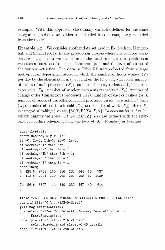
April 29, 2009 11:50 World Scientific Book - 9in x 6in Regression˙master
178 Linear Regression Analysis: Theory and Computing
example. With this approach, the dummy variables defined for the samecategorical predictor are either all included into or completely excludedfrom the model.
Example 5.2 We consider another data set used in Ex. 6.4 from Menden-hall and Sinich (2003). In any production process where one or more work-ers are engaged in a variety of tasks, the total time spent in productionvaries as a function of the size of the work pool and the level of output ofthe various activities. The data in Table 5.5 were collected from a largemetropolitan department store, in which the number of hours worked (Y )per day by the clerical staff may depend on the following variables: numberof pieces of mail processed (X1), number of money orders and gift certifi-cates sold (X2), number of window payments transacted (X3), number ofchange order transactions processed (X4), number of checks cashed (X5),number of pieces of miscellaneous mail processed on an “as available” basis(X6), number of bus tickets sold (X7) and the day of work (X8). Here, X8
is categorical taking 6 values M, T, W, Th, F, S. To account for it, five 0-1binary dummy variables Zt, Zw,Zth, Zf, Zs are defined with the refer-ence cell coding scheme, leaving the level of ‘M ’ (Monday) as baseline.
data clerical;
input weekday $ y x1-X7;
Zt =0; Zw=0; Zth=0; Zf=0; Zs=0;
if weekday="T" then Zt= 1;
if weekday="W" then Zw = 1;
if weekday="Th" then Zth = 1;
if weekday="F" then Zf = 1;
if weekday="S" then Zs = 1;
datalines;
M 128.5 7781 100 886 235 644 56 737
T 113.6 7004 110 962 388 589 57 1029
......
Th 86.6 6847 14 810 230 547 40 614
;
title "ALL POSSIBLE REGRESSIONS SELECTION FOR CLERICAL DATA";
ods rtf file="C:\...\SAS-5-2.rtf";
proc reg data=clerical;
ods select SelParmEst SelectionSummary RemovalStatistics
EntryStatistics;
model y = x1-x7 Zt Zw Zth Zf Zs/
selection=backward slstay=0.05 details;
model Y = x1-x7 Zt Zw Zth Zf Zs/

April 29, 2009 11:50 World Scientific Book - 9in x 6in Regression˙master
Model Selection 179
selection=forward slentry=0.05 details=steps;
model Y = x1-x7 Zt Zw Zth Zf Zs/selection=stepwise
slentry=0.05 slstay=0.05 details=summary;
run;
ods rtf close;
The above SAS program shows how to perform stepwise selection whilekeeping the five dummy variables processed in a groupwise manner. Notethat this groupwise method, unfortunately, is not available for the all pos-sible regressions selection method.
Table 5.6 presents the results from backward elimination. The vari-ables dropped from the model are X7, X1, X2, X3, and X4 in the order ofelimination. In every step, the dummy variables Zt, Zw, Zth, Zf , Zs areevaluated altogether with an F test. The final model in penal (b) selectsX5, X6, and the categorical predictor. ¤
Another alternative SAS procedure for linear regression is PROC GLM.The CLASS statement in PROC GLM automatically define dummy vari-ables for categorical predictors. However, it does not have the facility forautomatic model selection. One has to get around by writing macros orapplying a number of MODEL statements interactively.
5.5 Other Related Issues
Model selection is crucial and fundamental in statistical analysis. Whenevera statistical model, simple or complicated, is attempted, one has to face theissue of model identification. Its general scope, much broader than selectingthe best subset of variables, ranges from variable screening, throughoutbandwidth selection in kernel smoothing, tree size selection in decision trees,weight decay in neural networks and etc., to model ensemble methods suchas boosting. On the other hand, model selection is tricky and sometimescontroversial. It is common to see different selection methods result in quitedifferent model choices.
In the analysis of large data sets, variable screening is an important pre-liminary step. Very often it has been overlooked from classical statisticaltextbooks. But it is critical for practical data analysis. Mainly motivatedby fear of information loss and desire to optimize the profit of the experi-ment, investigators always try to collect as much information as they couldin a study. The resultant data set is often of enormous size, both in number
April 29, 2009 11:50 World Scientific Book - 9in x 6in Regression˙master
180 Linear Regression Analysis: Theory and Computing
of observations and number of variables, so that sometimes a simple com-putation of sample means may take seconds or minutes. This is not entirelyunrealistic when, for example, it comes to data mining practices. In thesescenarios, applying a modeling package directly could be overwhelminglyexpensive in computation. Variable screening helps identify and removepredictors that are not of much predictive values to the response.
Nevertheless, one should, in actuality, be cautious about dropping vari-ables. This is because data collection on these variables has been costly.Moreover, the relationships with the response can be of complicated formsand hard to decipher. Thus we suggest to try out a number of differentvariable screening techniques in order to facilitate a comprehensive evalua-tion on each predictor. Only these making it to the top drop list for all ormost screening methods can then be considered for exclusion.
In this section, we discuss several commonly used variable screeningmethods. There have also been quite a few recent advances in model se-lection. Among others, two fruitful developments are particularly remark-able: least absolute shrinkage and selection operator (LASSO) and Bayesianmodel averaging (BMA). We shall postpone their coverage to later chapters.The LASSO technique, covered in Chapter 7, makes available a continuousvariable selecting process. The BMA, discussed in Section 9.2, is intendedto integrate the uncertainties revolving around all candidate models.
5.5.1 Variance Importance or Relevance
The correlation of coefficient between each predictor and the response pro-vides a numerical summary of how they are linearly related. Variableswith a very small absolute correlation can potentially be screened out intothe removal list. One might also compute correlations or the variance in-flation factors (VIF) among predictors to identify those redundant ones.Recall that the VIF technique helps find out variables that can be mostlyaccounted for by linear combinations of other variables.
The concept of variable importance or relevance initially emerges fromthe machine learning literatures. It ranks all variables in order of theirimportance or relevance by fully examining the predictive power furnishedby each variable. The variable importance ranking feature provided inrandom forests (RF) (Breiman, 2001), which is among the newest and mostpromising developments in this regards, has been increasingly applied asa tool for variable selection in various fields. The method takes a cost-of-exclusion approach, in which the relevance of a variable is assessed by

April 29, 2009 11:50 World Scientific Book - 9in x 6in Regression˙master
Model Selection 181
01
02
03
04
05
0
(a) Random Forests
predictor
% In
cre
ase
in M
SE
x1 x2 x3 x4 x5
−0
.01
0.0
10
.02
0.0
30
.04
0.0
50
.06
(b) RELIEF
predictor
rele
van
ce
x1 x2 x3 x4 x5
Fig. 5.2 Variable Importance for the Quasar Data: Random Forests vs. RELIEF.
comparing some model performance measure with and without the givenfeature included in a modeling process. To approximate the underlyingregression function, random forests averages piecewise constants furnishedby a number of tree models.
The tree method, also called recursive partitioning, was first proposed byMorgan and Sonquist (1963). By recursively bisecting the predictor space,the hierarchical tree structure partitions the data into meaningful groups

May 7, 2009 10:22 World Scientific Book - 9in x 6in Regression˙master
182 Linear Regression Analysis: Theory and Computing
and makes available a piecewise approximation of the underlying relation-ship between the response and its associated predictors. The applicationsof tree models have been greatly advanced in various fields especially sincethe development of classification and regression trees (CART) by Breimanet al. (1984). Tree construction in CART consists of three major steps:(1) growing a large initial tree; (2) a pruning algorithm; and (3) a valida-tion method for determining the best tree size. The pruning idea for treesize selection in CART has become and remains the current standard inconstructing tree models.
Recursive partitioning, together with its various extensions such asMARS, bagging, boosting, and random forests, has come into play veryactively in modern statistical modeling and data mining practice. A de-tailed coverage of this techniques is beyond the scope. We refer interestedreaders to Breiman et al. (1984) and Breiman (2001) for a full accountof trees and random forests. The variable importance ranking in randomforests (RF) is available from the R package randomForest.
With the advent of modern computing facilities, various feature selec-tion algorithms have been proposed and studied in the field of machinelearning and data mining. Among others, the RELIEF algorithm devel-oped by Kira and Rendel (1992), Kononenko, Simec, and Robnik-Sikonja(1997), and Robnik-Sikonja and Kononenko (1997) is particularly worthmentioning. RELIEF ranks the relevance of each feature or variable by ac-cumulatively collecting information on its ability to distinguish responses ofdifferent values and agree on responses of similar values or patterns acrosssets of neighborhoods. Here, we shall only outline the RELIEF algorithminitially proposed for classification problems where the response variable Y
is binary. A handy way of how to apply it to data with continuous responsesis described in the example.
Suppose that the data set available consists of (yi,xi) : i = 1, . . . , n,where yi is the binary outcome with value being 0 or 1 and xi ∈ Rp isa p-dimensional predictor vector. The RELIEF algorithm is illustrated inAlgorithm 5.1. At each step of an iterative process, an instance is chosen atrandom from the data set and the importance measure for each variable isupdated according to how well it recognizes distanced and similar responsevalues.

May 7, 2009 10:22 World Scientific Book - 9in x 6in Regression˙master
Model Selection 183
Algorithm 5.1: RELIEF for Data with Binary Responses.
• Initialize all importance measures Wj = W (Xj) = 0 for j =1, 2, . . . , p;
• Do k = 1, 2, . . . , K
– Randomly select an observation k : (yk,xk), call it “Obs-k”;– Find the observation m, called ‘the nearest miss’ , which is closest,
in terms of the distance in x, to “Obs-k” and has response ym equalto yk;
– Find the observation h, called ‘the nearest hit’ , which is closest,in terms of the distance in x, to “Obs-k” and has response yh
unequal to yk;– Do j = 1, 2, . . . , p,
Update Wj ←−Wj − diff(xkj , xmj)/m + diff(xkj , xhj)/m;
– End do;
• End do.
In the outlined algorithm, function diff(xkj , xk′j) computes the differ-ence between xkj and xk′j , the values of predictor Xj for observations k andk′. While various distance definitions can apply to measure the difference,it is defined in the original proposal, for categorical predictors, as
diff(xkj , xk′j) =
0 if xkj = xk′j
1 otherwiseand for continuous predictors as
diff(Xkj , Xk′j) =|xkj − xk′j |
max(Xj)−min(Xj),
where max(Xj) and min(Xj) are the maximum and minimum of Xj , re-spectively. With this formulation, it is no need to normalize or standardizevariables that are measured in different scales. An implementation of RE-LIEF is available in R package: dprep.
Example We use the quasar data again to illustrate the two variableimportance ranking techniques. Figure 5.2 (a) plots the importance, mea-sured by percentage of increase in MSE, for each predictor from a 2,000random trees. Although it has been extended to continuous responses,the initial rationale in RELIEF works best in classification problems withbinary responses. One simple alternative way is to dichotomize the contin-uous response y into two classes by some randomly selected cutoff point,then proceed with RELIEF as if it is a classification problem. Repeat the

May 7, 2009 10:22 World Scientific Book - 9in x 6in Regression˙master
184 Linear Regression Analysis: Theory and Computing
procedure for multiple times, each time with different cutoff points, andfinally integrate the results by averaging the importance measures.
Figure 5.2 (b) plots the averaged relevance measure of each variableobtained from RELIEF in the manner just described. Since the samplesize n = 25 is small, two classes are used with 500 repetitions and, at eachrepetition, five randomly selected observations are used for computing therelevance. It can be seen that the two methods match somehow in theirfindings, both ranking X4 and X5 higher than others, except for that RFfound X4 as the most important while X5 is deemed most important byRELIEF.
While the variable importance techniques in RF packages are becomingvery popular due to their novelty and nonparametric nature, we would liketo call the reader’s attention to a selection bias problem brought up by,e.g., Strobl et al. (2007). It has been found that continuous predictors andcategorical predictors are treated differently. In particular, a variable thathas more distinct values or levels tends to be more weighted than a variablethat has much fewer distinct values or levels. This is an inherent problemin recursive partitioning, as a predictor with more distinct values generatesa much larger number of permissible splits. To put it in another way, ifone would like to apply some kind of critical values to signal the statisticalsignificance for the importance measures, the critical value can be quitedifferent for different predictors. Thus great caution should be exercisedwhen comparing the importance measures cross predictors.
To illustrate, we consider a simple simulation study on classification. Inthis study, each data set contains four covariates (X1, X2, X3, X4), none ofwhich is really related to a binary response Y . Here, X1 is binary takingvalues 0 and 1; X2 is categorical with 10 levels; X3 is continuous with valuesbeing randomly taken from 0.0, 0.1, . . . , 1.0; X4 is continuous with valuesin 0.00, 0.01, . . . , 1.00; and the response Y is generated independently as(+1,−1) with pr(Y = +1) = pr(Y = −1) = 0.5. Two sample sizes areconsidered: n = 100 and n = 1000. For each generated data sets, bothRELIEF and RF are applied to extract variable importance.
Figure 5.3 gives boxplots of the resultant importance measures obtainedin 200 simulation runs. For random forests, the Gini importance, whichdescribes the improvement in the “Gini gain” splitting criterion, is used. Wecan see that X2 is systematically weighted more than X1 merely due to morelevels it has. Similar behaviors can be observed for the comparison betweenX4 over X3. This selection bias problem remains even with increased samplesize. On the other hand, RELIEF does not seem to suffer much from this

April 29, 2009 11:50 World Scientific Book - 9in x 6in Regression˙master
Model Selection 185
X1 X2 X3 X4
0.0
0.2
0.4
0.6
(a) RELIEF n=100
X1 X2 X3 X4
51
01
52
0
(b) RF n=100
X1 X2 X3 X4
0.0
00
0.0
05
0.0
10
(a) RELIEF n=1000
X1 X2 X3 X4
50
10
01
50
20
0
(b) RF n=1000
Fig. 5.3 A Simulation Example on Variable Importance: Random Forests vs. RELIEF.
bias problem. The relevance measures it provided stay around 0 for allfour predictors, although variations of the measures for categorical andcontinuous variables are inherently different.
To amend the selection bias in random forests, Strobl et al. (2007), fol-lowing the series work of Loh (2002) in tree construction, suggests first se-
April 29, 2009 11:50 World Scientific Book - 9in x 6in Regression˙master
186 Linear Regression Analysis: Theory and Computing
lecting the most important variable at every split and then partitioning dataaccording to the most important variable selected. Furthermore, they foundthat subsampling without replacement, instead of bootstrapping, helps agreat deal in producing unbiased variable importance measures. This isbecause subsampling without replacement tends to yield less correlated im-portance measures. Alternatively, one might consider obtaining a criticalvalue for each variable to refer to by efficient use of permutation.
5.5.2 PCA and SIR
Dimension reduction techniques can be useful for variable selection in somecircumstances. The classical principal component analysis (PCA) findsdirections or linear combinations of predictors, atx, that explain most ofthe variations in predictors. Note that PCA is executed with no accountof the response. When applying PCA in regression problems, one is hopingthat the response also varies most in the directions that predictors varymost. A slightly more elaborated explanation on PCA can be found inSection 7.3.2.
Another technique, the sliced inverse regression (SIR), addresses dimen-sion reduction in regression directly. SIR assumes a multiple index modelgiven as
yi = f(at1xi, . . . ,at
Kxi, εi). (5.19)
Namely, y depends on x only through a set of indices. The dimension re-duction is achieved when K is much smaller than p, the dimension of x. Thespace spanned by ak’s, k = 1, . . . , K is called effective dimension reduction(EDR) space. Under fairly general conditions specified by Li (1991), it canbe shown that the standardized inverse regression curve E(Σ−1/2x|y) iscontained in the subspace spanned by Σ1/2ak’s, where Σ = Cov(x). ApplyPCA or spectral decomposition on matrix
Σ−1/2CovE(x|y)Σ−1/2 (5.20)
and let bk, for k = 1 . . . ,K, denotes the nonzero eigenvalues. The bk’sare the EDR directions spanning the EDR space. To compute bk, Σ isreplaced by the sample variance-covariance matrix of x and CovE(x|y)can be estimated by slicing the data according to y values. Alternatively,Li (1992) suggested to replace CovE(x|y) in (5.20) by
E[z− E(z)x− E(x)x− E(x)t
],

April 29, 2009 11:50 World Scientific Book - 9in x 6in Regression˙master
Model Selection 187
where the random vector z can be either the response vector y or theresidual vector obtained from a linear regression of y on x.
One remaining practical question is how the identified PCA or SIR di-rections can be used for regression or prediction. Plugging the PCA or SIRdirections directly into linear models is not a very appealing approach due tothe blurred interpretation. Two better model choices are projection pursuitregression (see, e.g., Friedman and Stuetzle, 1981) and neural networks (see,e.g., Bishop, 1995) when, in particular, the multi-layer perceptron (MLP)with one hidden layer is used. Both facilitate a ridge approximation to theunderlying regression function through models of the form
yi =K∑
k=1
gk(atkxi) + εi. (5.21)
A ridge function is referred to a function of some linear combination ofmultivariate components. While projection pursuit achieves nonparametricridge approximation with unspecified gk(·)’s, the neural networks model canbe viewed as a parametric version assuming that the functions gk(·) havea known form. The directions identified by PCA or SIR fit naturally intothese two modeling processes.

May 7, 2009 10:22 World Scientific Book - 9in x 6in Regression˙master
188 Linear Regression Analysis: Theory and Computing
Problems
1. Verify the following properties of partitioned matrices. Given a sym-metric p.d. matrix A is partitioned in the form
A =(
A11 A12
A21 A22
),
where A11 and A22 are square matrices, both A11 and A22 are p.d.and the inverse of A is given by
A−1 =(
A11 + A−111 A12B−1A21A−1
11 −A−111 A12B−1
−BA21A−111 B−1
),
with B = A22 −A21A−111 A12. Besides, by straightforward algebra, one
can verify that
(x′1 x′
2 ) A−1
(x1
x2
)= x′
1A−111 x1 + b′B−1b,
where b = x2 −A21A−111 x1.
2. Complete the remaining steps in the proof of Theorem 5.2.
3. Use the following simulation experiment (Cook and Weisberg, 1999,pp. 280-282) to inspect how stepwise selection overstates significance.Generate a data set of n = 100 cases with a response and 50 predictors,all from the standard normal distribution independently. Thus none ofthe predictors is really related to the response. Fit the following threemodels: a, Including all 50 predictors, fit the whole model withoutselection; b, obtain the final model by performing a forward additionprocedure with αentry = 0.25; c, Obtain the final model by performing aforward addition procedure with αentry = 0.05. Repeat the experimentwith n = 1, 000. Use Table 5.7 to summarize your results and makecomments.
4. The variance of the regression prediction and variance of the leastsquares estimators tend to be larger when the regression model is over-fitted. Show the following results for an over-fitted regression model:
(a) Let x1, x2, · · · , xk be the regressors and b0, b1, · · · , bk be the esti-mates of the regression model, if (k + 1)-th regressor xk+1 is addedinto the model and the estimates are denoted by b∗0, b
∗1, · · · , b∗k, b∗k+1
thenVar(b∗i ) ≥ Var(bi) for i = 0, 1, 2, · · · , k.

April 29, 2009 11:50 World Scientific Book - 9in x 6in Regression˙master
Model Selection 189
(b) The variance of fitted value based on an over-fitted model is larger.i.e., denote y1 =
∑ki=0 bixi and y2 =
∑k+1i=0 b∗i xi, then
Var(y1) ≤ Var(y2).
5. Consider the quasar data used in Example 5.1. Define Y ′ = log(Y ).Perform variable selection via both the all possible regressions methodand the three stepwise procedures. Examine the results and make com-ments.
6. All-subset-regression approach is an exhausted search and it is feasi-ble only in situation where the number of the regressors is not toolarge. Table 5.8 is the female teacher effectiveness data that has 7 in-dependent variables. In the data set, the response variable y is thequantitative evaluation made by the cooperating female teachers andthe regressors are the scores of the seven standard tests. Then theall-subset-regression approach would search for 27− 1 = 127 regressionmodels if the regression model with no regressors is excluded. Using theSAS procedure REG and PRESS criteria to verify among all possible127 regression models that the best regression models containing one,two, · · · , seven regressors are the models in Table 5.9.
7. As a criterion for comparing models, The Cp measure in (5.18) canalternatively be given by
Cp ≈ MSE +2 · (p + 1)
nσ2.
Suppose that MSE from the current model is used to estimate the truenoise variance, i.e., σ2 = MSE. Show that Cp is similar to the GCVcriterion given in (5.10), using approximation
11− x2
≈ 1 + 2x.

April 29, 2009 11:50 World Scientific Book - 9in x 6in Regression˙master
190 Linear Regression Analysis: Theory and Computing
Table 5.3 Backward Elimination Procedure for the Quasar Data.
(a) Steps in backward elimination.
Step 0: The Full Model
Parameter Standard Type II F TestVariable Estimate Error SS Value P-Value
Intercept −33.9611 11.64951 0.00040842 8.50 0.0089X1 −0.0295 0.04481 0.00002081 0.43 0.5184X2 1.4690 0.36414 0.00078215 16.28 0.0007X3 0.8549 0.36184 0.00026828 5.58 0.0290X4 0.9662 0.25139 0.00070989 14.77 0.0011X5 −0.0400 0.25021 0.00000123 0.03 0.8746
Step 1: After Removing X5
Parameter Standard Type II F TestVariable Estimate Error SS Value P-Value
Intercept −35.2616 8.1375 0.00085839 18.78 0.0003X1 −0.0262 0.0389 0.00002075 0.45 0.5082X2 1.4154 0.1386 0.00477 104.30 < .0001X3 0.9080 0.1407 0.00190 41.65 < .0001X4 0.9260 0.0028 5.17789 113264 < .0001
Step 2: After Removing X1
Parameter Standard Type II F TestVariable Estimate Error SS Value P-Value
Intercept −29.79820 0.67081 0.08786 1973.23 < .0001X2 1.50849 0.01102 0.83506 18754.3 < .0001X3 0.81358 0.01223 0.19706 4425.58 < .0001X4 0.92575 0.00269 5.28153 118615 < .0001
(b) Summary of Backward Elimination.
Variable Num of Vars Partial Model F TestStep Removed in Model R-Square R2 Cp Value P-Value
1 X5 4 0.0000 0.9998 4.0256 0.03 0.87462 X1 3 0.0000 0.9998 2.4574 0.45 0.5082
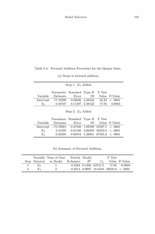
April 29, 2009 11:50 World Scientific Book - 9in x 6in Regression˙master
Model Selection 191
Table 5.4 Forward Addition Procedure for the Quasar Data.
(a) Steps in forward addition.
Step 1: X5 Added
Parameter Standard Type II F TestVariable Estimate Error SS Value P-Value
Intercept 17.19298 3.02830 4.29432 32.23 < .0001X5 0.48707 0.11497 2.39122 17.95 0.0003
Step 2: X3 Added
Parameter Standard Type II F TestVariable Estimate Error SS Value P-Value
Intercept −75.76681 0.47440 1.98599 25507.5 < .0001X3 2.31295 0.01166 3.06250 39333.9 < .0001X5 0.92205 0.00354 5.28081 67825.2 < .0001
(b) Summary of Forward Addition.
Variable Num of Vars Partial Model F TestStep Entered in Model R-Square R2 Cp Value P-Value
1 X5 1 0.4383 0.4383 63741.5 17.95 0.00032 X3 2 0.5614 0.9997 16.6433 39333.9 < .0001

April 29, 2009 11:50 World Scientific Book - 9in x 6in Regression˙master
192 Linear Regression Analysis: Theory and Computing
Table 5.5 The Clerical Data from Ex. 6.4 in Mendenhall and Sinich (2003)
Day ofObs. Week Y X1 X2 X3 X4 X5 X6 X7
1 M 128.5 7781 100 886 235 644 56 7372 T 113.6 7004 110 962 388 589 57 10293 W 146.6 7267 61 1342 398 1081 59 8304 Th 124.3 2129 102 1153 457 891 57 14685 F 100.4 4878 45 803 577 537 49 3356 S 119.2 3999 144 1127 345 563 64 9187 M 109.5 11777 123 627 326 402 60 3358 T 128.5 5764 78 748 161 495 57 9629 W 131.2 7392 172 876 219 823 62 66510 Th 112.2 8100 126 685 287 555 86 57711 F 95.4 4736 115 436 235 456 38 21412 S 124.6 4337 110 899 127 573 73 48413 M 103.7 3079 96 570 180 428 59 45614 T 103.6 7273 51 826 118 463 53 90715 W 133.2 4091 116 1060 206 961 67 95116 Th 111.4 3390 70 957 284 745 77 144617 F 97.7 6319 58 559 220 539 41 44018 S 132.1 7447 83 1050 174 553 63 113319 M 135.9 7100 80 568 124 428 55 45620 T 131.3 8035 115 709 174 498 78 96821 W 150.4 5579 83 568 223 683 79 66022 Th 124.9 4338 78 900 115 556 84 55523 F 97 6895 18 442 118 479 41 20324 S 114.1 3629 133 644 155 505 57 78125 M 88.3 5149 92 389 124 405 59 23626 T 117.6 5241 110 612 222 477 55 61627 W 128.2 2917 69 1057 378 970 80 121028 Th 138.8 4390 70 974 195 1027 81 145229 F 109.5 4957 24 783 358 893 51 61630 S 118.9 7099 130 1419 374 609 62 95731 M 122.2 7337 128 1137 238 461 51 96832 T 142.8 8301 115 946 191 771 74 71933 W 133.9 4889 86 750 214 513 69 48934 Th 100.2 6308 81 461 132 430 49 34135 F 116.8 6908 145 864 164 549 57 90236 S 97.3 5345 116 604 127 360 48 12637 M 98 6994 59 714 107 473 53 72638 T 136.5 6781 78 917 171 805 74 110039 W 111.7 3142 106 809 335 702 70 172140 Th 98.6 5738 27 546 126 455 52 50241 F 116.2 4931 174 891 129 481 71 73742 S 108.9 6501 69 643 129 334 47 47343 M 120.6 5678 94 828 107 384 52 108344 T 131.8 4619 100 777 164 834 67 84145 W 112.4 1832 124 626 158 571 71 62746 Th 92.5 5445 52 432 121 458 42 31347 F 120 4123 84 432 153 544 42 65448 S 112.2 5884 89 1061 100 391 31 28049 M 113 5505 45 562 84 444 36 81450 T 138.7 2882 94 601 139 799 44 90751 W 122.1 2395 89 637 201 747 30 166652 Th 86.6 6847 14 810 230 547 40 614
a Source: Adapted from Work Measurement, by G. L. Smith, Grid PublishingCo., Columbus, Ohio, 1978 (Table 3.1).
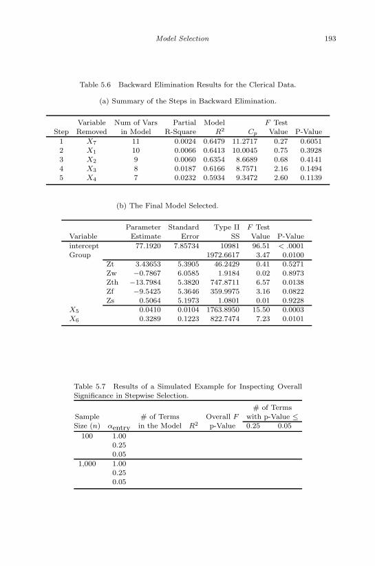
May 7, 2009 10:22 World Scientific Book - 9in x 6in Regression˙master
Model Selection 193
Table 5.6 Backward Elimination Results for the Clerical Data.
(a) Summary of the Steps in Backward Elimination.
Variable Num of Vars Partial Model F TestStep Removed in Model R-Square R2 Cp Value P-Value
1 X7 11 0.0024 0.6479 11.2717 0.27 0.60512 X1 10 0.0066 0.6413 10.0045 0.75 0.39283 X2 9 0.0060 0.6354 8.6689 0.68 0.41414 X3 8 0.0187 0.6166 8.7571 2.16 0.14945 X4 7 0.0232 0.5934 9.3472 2.60 0.1139
(b) The Final Model Selected.
Parameter Standard Type II F TestVariable Estimate Error SS Value P-Value
intercept 77.1920 7.85734 10981 96.51 < .0001Group 1972.6617 3.47 0.0100
Zt 3.43653 5.3905 46.2429 0.41 0.5271Zw −0.7867 6.0585 1.9184 0.02 0.8973Zth −13.7984 5.3820 747.8711 6.57 0.0138Zf −9.5425 5.3646 359.9975 3.16 0.0822Zs 0.5064 5.1973 1.0801 0.01 0.9228
X5 0.0410 0.0104 1763.8950 15.50 0.0003X6 0.3289 0.1223 822.7474 7.23 0.0101
Table 5.7 Results of a Simulated Example for Inspecting OverallSignificance in Stepwise Selection.
# of TermsSample # of Terms Overall F with p-Value ≤Size (n) αentry in the Model R2 p-Value 0.25 0.05
100 1.000.250.05
1,000 1.000.250.05

April 29, 2009 11:50 World Scientific Book - 9in x 6in Regression˙master
194 Linear Regression Analysis: Theory and Computing
Table 5.8 Female Teachers Effectiveness Data
y x1 x2 x3 x4 x5 x6 x7Effectiveness Standard Standard Standard Standard Standard Standard Standard
Score Test 1 Test 2 Test 3 Test 4 Test 5 Test 6 Test 7
410 69 125 93 3.70 59.00 52.5 55.66569 57 131 95 3.64 31.75 56.0 63.97425 77 141 99 3.12 80.50 44.0 45.32344 81 122 98 2.22 75.00 37.3 46.67324 0 141 106 1.57 49.00 40.8 41.21505 53 152 110 3.33 49.35 40.2 43.83235 77 141 97 2.48 60.75 44.0 41.61501 76 132 98 3.10 41.25 66.3 64.57400 65 157 95 3.07 50.75 37.3 42.41584 97 166 120 3.61 32.25 62.4 57.95434 76 141 106 3.51 54.50 61.9 57.90
Data Source: Raymond H. Myers, Classical and Modern Regression with Applications.Duxbury, p. 191.
Table 5.9 All-subset-regression for Female Teacher Effectiveness Data
Vars Intercept x1 x2 x3 x4 x5 x6 x7 CP PRESS
x7 14.72 . . . . . . 8.14 23.71 82293x2x7 -577.84 . 3.73 . . . . 9.47 12.42 51498x2x6x7 -911.68 . 5.48 . . . -10.10 20.97 5.64 35640.82x1x2x6x7 -920.41 -0.32 5.57 . . . -10.00 21.22 7.35 40279.35x1x2x5x6x7 -1654.82 -1.32 8.16 . . 3.24 -11.64 27.96 6.81 34607.30x1x2x4x5x6x7 -1510.98 -1.42 7.44 . 22.80 2.89 -10.69 25.37 8.38 42295x1x2x3x4x5x6x7 -1499.47 -1.22 5.05 4.10 39.44 2.24 -11.54 23.79 8.00 115019

April 29, 2009 11:50 World Scientific Book - 9in x 6in Regression˙master
Chapter 6
Model Diagnostics:Heteroscedasticity and Linearity
Model diagnostics involve two aspects: outlier detection and model assump-tion checking. In Chapter 4, we have discussed various criteria on how todetect regression outliers that have unusual response or predictor valuesand influential observations whose inclusion in the data set would havesubstantial impact on model estimation and prediction. In this chapter,we continue to study the second aspect of model diagnostics, i.e., how toevaluate the validity of model assumptions and how to make remedies ifany of the model assumptions is found violated.
There are four major assumptions involved in the classical linear regres-sion model:
y = Xβ + ε with ε ∼ N (0, σ2I), (6.1)
where X is n× (k + 1) of rank (k + 1). These are listed below.
• Linearity : The linearity assumption is referred to as the assumed linearrelationship between the mean response E(yi|xi) and the predictors xi.
It is this assumption that leads to E(εi) = 0.
• Independence: The independence assumption states that the observa-tions in the data set are randomly selected, which corresponds to theindependence of random errors.
• Homoscedasticity : The homoscedasticity assumption requires that allrandom errors have the same constant variance.
• Normality : Normally distributed random errors are assumed.
All the four assumptions can be summarized in short by εiiid∼ N (0, σ2) for
i = 1, . . . , n.
We shall briefly discuss how to check the independence and normal-ity assumptions. Among these four, the independence assumption is the
195

April 29, 2009 11:50 World Scientific Book - 9in x 6in Regression˙master
196 Linear Regression Analysis: Theory and Computing
hardest to check. There are only a couple of limited tests available for test-ing independence. For example, the Durbin-Watson test, which tests forautocorrelation, is discussed on page 235 and illustrated on page 266. Nev-ertheless, the plausibility of independence usually can be inspected fromdata collection schemes. If data are collected by simple random sampling,it is reasonable to assume independence. If, on the other hand, the data arecollected over time in a longitudinal study or several measures are taken re-peatedly from the same unit in a cluster study, then the dependence amongobservations becomes manifest and should not be ignored. Random and/ormixed effect models (McCulloch, Searle, and Neuhaus, 2008) are often usedto model the intra-cluster correlation or time-related dependence structure.
The normality assumption can be checked (see Section 3.17) by graph-ically or numerically examining the studentized jackknife residuals,
r(−i) =yi − yi√
MSE(−i) · (1− hii)= ri
√(n− 1)− (k + 1)n− (k + 1) − r2
i
, (6.2)
where MSE(−i) is the resultant MSE from fitting the linear model withi-th observation excluded; hii is the i-th leverage; and
ri =yi − yi√
MSE · (1− hii)is the i-th studentized residual. Under the model assumptions, it can beshown that r(−i) follows the t distribution with (n− 1)− (k + 1) degreesof freedom, which be approximated by N (0, 1) for large dfs. Graphically,the quantile-quantile (or Q-Q) normal probability plot of the studentizedjackknife residuals can be used to examine normality. Numerically, variousgoodness-of-fit tests can be used to formally test for normality. The mostcommonly used one, for example, is the Shapiro-Wilk test, which is availablein PROC UNIVARIATE with the NORMAL option in SAS and in the Rfunction shapiro.test(). Nevertheless, we would like to comment thatthe normality assumption is of somewhat lesser concern for large data inthe spirit of the central limit theorem. The inferences in linear regressionshow considerable robustness to violation of normality as long as the samplesize is reasonably large.
However, the two other assumptions, linearity and homoscedasticity,are closely related to the bias and variance in model estimation. Viola-tion of either assumption may result in severely misleading results. Theerrors induced by misspecified homoscedasticity or linearity will not belessened with increased sample size and the problems remain for large sam-ples. In this chapter, we shall consider tests for assessing homoscedasticityand strategies for exploring the appropriate functional form.

April 29, 2009 11:50 World Scientific Book - 9in x 6in Regression˙master
Model Diagnostics 197
6.1 Test Heteroscedasticity
In classical regression, the equal variance assumption simply states that,given X, the conditional variance of the error terms are constant for all ob-servations. In other words, whenever X varies, the corresponding responseY has the same variance around the regression line. This is so-called ho-moscedasticity. Referring to the weighted least square estimation in Section7.2.4, this assumption implies that all Y values corresponding to variousX’s are equally important and should be evenly weighted. In contrast, thecondition of the error variance not being constant over all observations iscalled heteroscedasticity.
6.1.1 Heteroscedasticity
In statistics, a sequence or a vector of random variables is said to be het-eroscedastic, if the random variables have different variances. When sta-tistical techniques, such as the ordinary least squares (OLS), is applied tothe regression model, a number of assumptions are typically made. Oneof these is that the error term in the model has a constant variance. Thiswill be true if the observations of the error term are assumed to be drawnfrom identical distributions. Heteroscedasticity is the violation of this as-sumption. What is the validity of this assumption and what happens ifthis assumption is not fulfilled? Specifically, the following questions can beasked:
1. What is the nature of heteroscedasticity?2. What are the consequences of heteroscedasticity?3. How do we detect heteroscedasticity?4. How do we control for heteroscedasticity?
In general, there are several reasons why stochastic disturbance termsin the model may be heteroscedastic:
1. Response variable may change its magnitude according to the valuesof one or more independent variables in the model. Therefore, it mayinduce heteroscedastic error.
2. As data collecting techniques improve, it is likely to decrease the vari-ation and to commit fewer errors.
3. Outlier observations are much different in relation to the other obser-vations in the sample. The inclusion or exclusion of such observations,
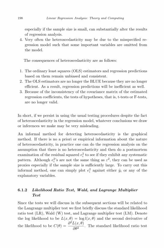
April 29, 2009 11:50 World Scientific Book - 9in x 6in Regression˙master
198 Linear Regression Analysis: Theory and Computing
especially if the sample size is small, can substantially alter the resultsof regression analysis.
4. Very often the heteroscedasticity may be due to the misspecified re-gression model such that some important variables are omitted fromthe model.
The consequences of heteroscedasticity are as follows:
1. The ordinary least squares (OLS) estimators and regression predictionsbased on them remain unbiased and consistent.
2. The OLS estimators are no longer the BLUE because they are no longerefficient. As a result, regression predictions will be inefficient as well.
3. Because of the inconsistency of the covariance matrix of the estimatedregression coefficients, the tests of hypotheses, that is, t-tests or F-tests,are no longer valid.
In short, if we persist in using the usual testing procedures despite the factof heteroscedasticity in the regression model, whatever conclusions we drawor inferences we make may be very misleading.
An informal method for detecting heteroscedasticity is the graphicalmethod. If there is no a priori or empirical information about the natureof heteroscedasticity, in practice one can do the regression analysis on theassumption that there is no heteroscedasticity and then do a postmortemexamination of the residual squared e2
i to see if they exhibit any systematicpattern. Although e2
i ’s are not the same thing as ε2, they can be used asproxies especially if the sample size is sufficiently large. To carry out thisinformal method, one can simply plot e2
i against either yi or any of theexplanatory variables.
6.1.2 Likelihood Ratio Test, Wald, and Lagrange Multiplier
Test
Since the tests we will discuss in the subsequent sections will be related tothe Langrange multiplier test we first briefly discuss the standard likelihoodratio test (LR), Wald (W) test, and Lagrange multiplier test (LM). Denotethe log likelihood to be L(x, θ) = log l(x, θ) and the second derivative of
the likelihood to be C(θ) =∂2L(x, θ)
∂θ2. The standard likelihood ratio test

April 29, 2009 11:50 World Scientific Book - 9in x 6in Regression˙master
Model Diagnostics 199
is defined as
LR = 2[log l(x, θ)− log l(x, θ)], (6.3)
where θ is the likelihood estimate without restrictions, θ is the likelihoodestimate with restrictions, and g is the number of the restrictions imposed.The asymptotic distribution of the LR test is the χ2 with g degrees offreedom. The Wald test is defined as
W = (θ − θ0)′I(θ)(θ − θ0), (6.4)
where I(θ) = Eθ
[∂2 log l(x, θ)∂θ2
], the information matrix.
The basic idea of the Lagrange multiplier test focuses on the characteristicof the log-likelihood function when the restrictions are imposed on the nullhypothesis. Suppose that the null hypothesis is H0 : β = β0, we considera maximization problem of log-likelihood function when the restriction ofthe null hypothesis which we believe to be true is imposed. That is, wetry to solve for maximization problem under the constrain β = β0. Thisrestricted maximization problem can be solved via the Lagrange multipliermethod. i.e., we can solve for the unconstrained maximization problem:
maxβ
[L(β) + λ(β − β0)
].
Differentiating with respect to β and λ and setting the results equal tozero yield the restricted maximum likelihood estimation, β∗ = β0, and theestimate of the Lagrange multiplier, λ∗ = S(β∗) = S(β0), where S(·) is
the slope of the log-likelihood function, S(β) =dL(β)
dβ, evaluated at the
restricted value β0. The greater the agreement between the data and thenull hypothesis, i.e., β ≈ β0, the closer the slope will be to zero. Hence,the Lagrange multiplier can be used to measure the distance between β
and β0. The standard form for the LM test is defined as
LM = [S(θ0)]2I(θ0)−1 ∼ χ21 (6.5)
The generalization to the multivariate version is a straightforward extensionof (6.5) and can be written as
LM = S(θ)′I(θ)−1S(θ) ∼ χ2
g, (6.6)
where g is the number of linear restrictions imposed.

April 29, 2009 11:50 World Scientific Book - 9in x 6in Regression˙master
200 Linear Regression Analysis: Theory and Computing
Example We now give an example to compute the LR, Wald, and LMtests for the elementary problem of the null hypothesis H0 : µ = µ0 againstHa : µ 6= µ0 from a sample size n drawn from a normal distribution withvariance of unity. i.e., X ∼ N(µ, 1) and the log-likelihood function is
L(µ) = −n
2log(2π)− 1
2
n∑
i=1
(Xi − µ)2,
which is a quadratic form in µ. The first derivative of the log-likelihood is
dL(µ)dµ
=n∑
i=1
(Xi − µ) = n(X − µ),
and the first derivative of the log-likelihood is a quadratic form in µ. Thesecond derivative of the log-likelihood is a constant:
d2L(µ)dµ2
= −n.
The maximum likelihood estimate of µ is µ = X and LR test is given by
LR = 2[L(µ)− L(µ0)]
=n∑
i=1
(Xi − µ0)2 −n∑
i=1
(Xi − X)2
= n(X − µ0)2. (6.7)
The Wald test is given by
W = (µ− µ0)2I(θ0) = n(X − µ0)2. (6.8)
SincedL(µ0)
dµ= n(X − µ0), the LM test is given by
W = S(µ0)2C(θ0)−1 = n(X − µ0)2. (6.9)
Note that X ∼ N(µ0, n−1), each statistic is the square of a standard normal
variable and hence is distributed as χ2 with one degree of freedom. Thus,in this particular example the test statistics are χ2 for all sample sizes andtherefore are also asymptotically χ2
1. ¤

April 29, 2009 11:50 World Scientific Book - 9in x 6in Regression˙master
Model Diagnostics 201
6.1.3 Tests for Heteroscedasticity
There are several formal tests that can be used to test for the assumptionthat the residuals are homoscedastic in a regression model. White’s (1980)test is general and does not presume a particular form of heteroscedasticity.Unfortunately, little can be said about its power and it has poor smallsample properties unless there are very few number of regressors. If we haveprior knowledge that the variance σ2
i is a linear (in parameters) function ofexplanatory variables, the Breusch-Pagan (1979) test is more powerful. Inaddition, Koenker (1981) proposes a variant of the Breusch-Pagan test thatdoes not assume normally distributed errors. We explain these methods asfollows.
6.1.3.1 White’s Test
In statistics, White’s test (1980), named after Halbert White, is a testwhich establishes whether the variance in a regression model is constant(homoscedasticity). To test for constant variance we regresses the squaredresiduals from a regression model onto the regressors, the cross-products ofthe regressors, and the squared regressors. Then the White’s test statisticwill be used to perform the test. The White’s test does not require anyprior knowledge about the source of heteroscedasticity. It is actually alarge sample Lagrange Multiplier (LM) test, and it does not depend onthe normality of population errors. We use the regression model yi =β0 + β1x1i + β2x2i + εi to illustrate the White’s test.
(1) Given the data, estimate the regression model and obtain the residualsei = yi − yi.
(2) Next, estimate the following auxiliary regression model and obtain itsR2:
ei = β0 + β1x1i + β2x2i + β3x21i + β4x
22i + β5x1ix2i + εi.
(3) Compute White’s test statistic: Under the null hypothesis that there isno heteroscedasticity, it can be shown that the sample size n times theR2 obtained from the auxiliary regression asymptotically follows thechi-square distribution with degrees of freedom equal to the number ofregressors (not including the constant term) in the auxiliary regression.That is,
nR2 ∼ χ25.

April 29, 2009 11:50 World Scientific Book - 9in x 6in Regression˙master
202 Linear Regression Analysis: Theory and Computing
(4) Perform the test by comparing nR2 to the chi-square critical value.If nR2 > χ2
α, 5, the conclusion is that there is heteroscedasticity. IfnR2 < χ2
α, 5, there is no heteroscedasticity, which implies that
β1 = β2 = β3 = β4 = β5 = 0.
6.1.3.2 Park, Glesjer, and Breusch-Pagan-Godfrey Tests
All three of these tests are similar. Like White’s test, each of these testsis the Lagrange Multiplier (LM) test and thus follows the same generalprocedure. Given the regression model,
yi = β0 + β1x1i + β2x2i + · · ·+ βkxki + εi.
The Park, Glesjer, and Breusch-Pagan-Godfrey Tests carry out the follow-ing steps:
(1) Given the data, estimate the regression model and obtain the residuals,ei = yi − yi.
(2) Estimate the following auxiliary regression models and obtain theirR2’s.
(a) For Park Test the auxiliary regression model is:
log e2i = α0 + α1 log Z1i + α2 log Z2i + · · ·+ αp log Zpi + εi
(b) For Glesjer test the auxiliary regression is:
e2i = α0 + α1Z1i + α2Z2i + · · ·+ αpZpi + εi
(c) For Breusch-Pagan-Godfrey test the auxiliary regression is:
e2i = α0 + α1Z1i + α2Z2i + · · ·+ αpZpi + εi,
where e2i = e2
i /(∑n
i=1 e2i /n
). In each auxiliary regression, the Zi’s
may be some or all of the Xi’s.
(3) Compute the LM test statistic: Under the null hypothesis that there isno heteroscedasticity, it can be shown that the sample size n times theR2 obtained from the auxiliary regressions asymptotically follows thechi-square distribution with degrees of freedom equal to the number ofregressors (not including the constant term) in the auxiliary regressionmodel. That is,
nR2 ∼ χ2p.

April 29, 2009 11:50 World Scientific Book - 9in x 6in Regression˙master
Model Diagnostics 203
It is important to note that the test statistics originally proposed byPark and Glesjer are Wald test statistics, and the test statistic origi-nally suggested in the Breusch-Pagan-Godfrey Test is one-half of theauxiliary regressions explained sum of squares, distributed chi-squarewith p degrees of freedom. However, as pointed out by Engle (1984),since all of these tests are simply large-sample tests, they are all oper-ationally equivalent to the LM test.
(4) Perform the LM test by comparing nR2 to the chi-square critical value.If nR2 > χ2
α, p, the conclusion is that there is heteroscedasticity. IfnR2 < χ2
α, p, there is no heteroscedasticity, which implies that
α1 = α2 = · · · = αp = 0.
The Park, Glesjer, and Breusch-Pagan-Godfrey tests all require knowledgeabout the source of heteroscedasticity. i.e., the Z variables are known tobe responsible for the heteroscedasticity. These tests are all, in essence,LM tests. In the Park test, the error term in the auxiliary regression maynot satisfy the classical nonlinear regression model (CNLRM) assumptionsand may be heteroscedastic itself. In the Glejser test, the error term ei
is nonzero, is serially correlated, and is ironically heteroscedastic. In theBreusch-Pagan-Godfrey test, the error term is quite sensitive to the nor-mality assumption in small samples.
6.1.3.3 Goldfeld-Quandt test
If population errors are homoscedastic, and thus share the same varianceover all observations, then the variance of residuals from a part of the sam-ple observations should be equal to the variance of residuals from anotherpart of the sample observations. Thus, a “natural” approach to test for het-eroscedasticity would be to perform the F-test for the equality of residualvariances, where the F-statistic is simply the ratio of two sample variances.Consider the following regression model:
yi = β0 + β1x1i + β2x2i + · · ·+ βkxki + εi.
(1) Identify a variable to which the population error variance is related. Forillustrative purpose, we assume that X1 is related to Var(εi) positively.
(2) Order or rank the observations according to the values of X1, beginningwith the lowest X1 value.
(3) Omit c central observations, where c is specified a priori, and dividethe remaining n − c observations into two groups each of (n − c)/2

April 29, 2009 11:50 World Scientific Book - 9in x 6in Regression˙master
204 Linear Regression Analysis: Theory and Computing
observations. The choice of c, for the most part, is arbitrary; however,as a rule of thumb, it will usually lie between one-sixth and one-thirdof the total observations.
(4) Run separate regressions on the first (n − c)/2 observations and thelast (n − c)/2 observations, and obtain the respective residual sumof squares: ESS1 representing the residual sum of squares from theregression corresponding to the smaller X1 values (the small variancegroup) and ESS2 from the larger X1 values (the large variance group).
(5) Compute the F-statistic
F =ESS1/df
ESS2/df,
where df =n− c− 2(k + 1)
2and k is the number of estimated slope
coefficients.(6) Perform the F-test. If εi’s are normally distributed, and if the ho-
moscedasticity assumption is valid, then it can be shown that F fol-lows the F distribution with degrees of freedom in both the numeratorand denominator. If F > Fα, df, df , then we can reject the hypothe-sis of homoscedasticity, otherwise we cannot reject the hypothesis ofhomoscedasticity.
The Goldfeld-Quandt test depends importantly on the value of c and onidentifying the correct X variable with which to order the observations.This test cannot accommodate situations where the combination of severalvariables is the source of heteroscedasticity. In this case, because no singlevariable is the cause of the problem, the Goldfeld-Quandt test will likelyconclude that no heteroscedasticity exists when in fact it does.
6.2 Detection of Regression Functional Form
Despite all the favorable properties of linear regression, the effects of pre-dictors might be curvilinear in reality and the straight line can only offera rather poor approximation. The partial residual plot or the partial re-gression plot graphically helps depict the linear or nonlinear relationshipbetween the response and an individual predictor after adjusting for otherpredictors. However, eventually it would be preferable to have available anexplicit functional form that characterizes their relationship.
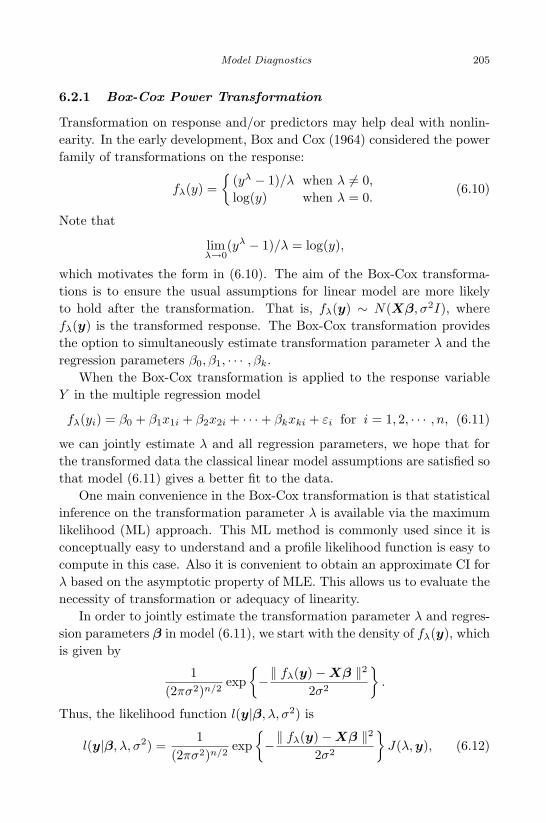
April 29, 2009 11:50 World Scientific Book - 9in x 6in Regression˙master
Model Diagnostics 205
6.2.1 Box-Cox Power Transformation
Transformation on response and/or predictors may help deal with nonlin-earity. In the early development, Box and Cox (1964) considered the powerfamily of transformations on the response:
fλ(y) =
(yλ − 1)/λ when λ 6= 0,
log(y) when λ = 0.(6.10)
Note that
limλ→0
(yλ − 1)/λ = log(y),
which motivates the form in (6.10). The aim of the Box-Cox transforma-tions is to ensure the usual assumptions for linear model are more likelyto hold after the transformation. That is, fλ(y) ∼ N(Xβ, σ2I), wherefλ(y) is the transformed response. The Box-Cox transformation providesthe option to simultaneously estimate transformation parameter λ and theregression parameters β0, β1, · · · , βk.
When the Box-Cox transformation is applied to the response variableY in the multiple regression model
fλ(yi) = β0 + β1x1i + β2x2i + · · ·+ βkxki + εi for i = 1, 2, · · · , n, (6.11)
we can jointly estimate λ and all regression parameters, we hope that forthe transformed data the classical linear model assumptions are satisfied sothat model (6.11) gives a better fit to the data.
One main convenience in the Box-Cox transformation is that statisticalinference on the transformation parameter λ is available via the maximumlikelihood (ML) approach. This ML method is commonly used since it isconceptually easy to understand and a profile likelihood function is easy tocompute in this case. Also it is convenient to obtain an approximate CI forλ based on the asymptotic property of MLE. This allows us to evaluate thenecessity of transformation or adequacy of linearity.
In order to jointly estimate the transformation parameter λ and regres-sion parameters β in model (6.11), we start with the density of fλ(y), whichis given by
1(2πσ2)n/2
exp−‖ fλ(y)−Xβ ‖2
2σ2
.
Thus, the likelihood function l(y|β, λ, σ2) is
l(y|β, λ, σ2) =1
(2πσ2)n/2exp
−‖ fλ(y)−Xβ ‖2
2σ2
J(λ, y), (6.12)
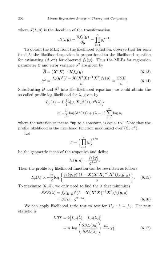
April 29, 2009 11:50 World Scientific Book - 9in x 6in Regression˙master
206 Linear Regression Analysis: Theory and Computing
where J(λ,y) is the Jocobian of the transformation
J(λ, y) =∂fλ(y)
∂y=
n∏
i=1
yλ−1i .
To obtain the MLE from the likelihood equation, observe that for eachfixed λ, the likelihood equation is proportional to the likelihood equationfor estimating (β, σ2) for observed fλ(y). Thus the MLEs for regressionparameter β and error variance σ2 are given by
β = (XtX)−1Xfλ(y) (6.13)
σ2 =fλ(y)t(I −X(XtX)−1Xt)fλ(y)
n=
SSE
n. (6.14)
Substituting β and σ2 into the likelihood equation, we could obtain theso-called profile log likelihood for λ, given by
Lp(λ) = L
λ|y, X, β(λ), σ2(λ)
∝ −n
2logσ2(λ)+ (λ− 1)
n∑
i=1
log yi,
where the notation ∝ means “up to a constant, is equal to.” Note that theprofile likelihood is the likelihood function maximized over (β, σ2).
Let
g =( n∏
i=1
yi
)1/n
be the geometric mean of the responses and define
fλ(y, g) =fλ(y)gλ−1
.
Then the profile log likelihood function can be rewritten as follows
Lp(λ) ∝ −n
2log
fλ(y, g)t(I −X(XtX)−1Xt)fλ(y, g)
n
. (6.15)
To maximize (6.15), we only need to find the λ that minimizes
SSE(λ) = fλ(y, g)t(I −X(XtX)−1Xt)fλ(y, g)
= SSE · g2−2λ. (6.16)
We can apply likelihood ratio test to test for H0 : λ = λ0. The teststatistic is
LRT = 2[LP (λ)− LP (λ0)
]
= n log
(SSE(λ0)
SSE(λ)
)H0−→ χ2
1. (6.17)
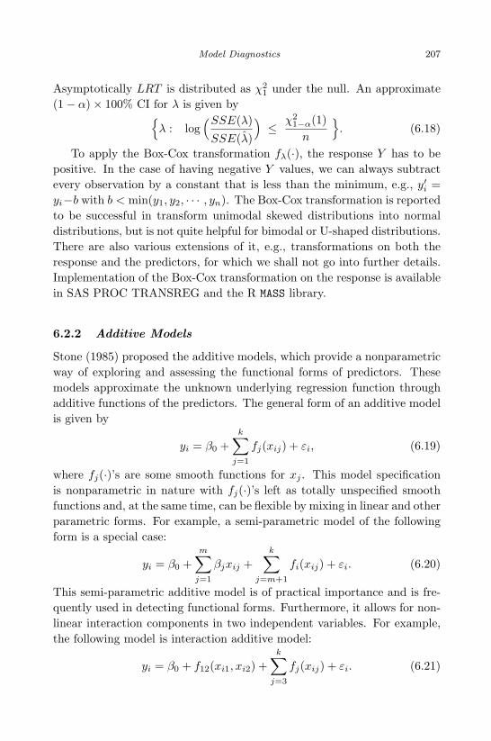
April 29, 2009 11:50 World Scientific Book - 9in x 6in Regression˙master
Model Diagnostics 207
Asymptotically LRT is distributed as χ21 under the null. An approximate
(1− α)× 100% CI for λ is given by
λ : log(SSE(λ)
SSE(λ)
)≤ χ2
1−α(1)n
. (6.18)
To apply the Box-Cox transformation fλ(·), the response Y has to bepositive. In the case of having negative Y values, we can always subtractevery observation by a constant that is less than the minimum, e.g., y′i =yi−b with b < min(y1, y2, · · · , yn). The Box-Cox transformation is reportedto be successful in transform unimodal skewed distributions into normaldistributions, but is not quite helpful for bimodal or U-shaped distributions.There are also various extensions of it, e.g., transformations on both theresponse and the predictors, for which we shall not go into further details.Implementation of the Box-Cox transformation on the response is availablein SAS PROC TRANSREG and the R MASS library.
6.2.2 Additive Models
Stone (1985) proposed the additive models, which provide a nonparametricway of exploring and assessing the functional forms of predictors. Thesemodels approximate the unknown underlying regression function throughadditive functions of the predictors. The general form of an additive modelis given by
yi = β0 +k∑
j=1
fj(xij) + εi, (6.19)
where fj(·)’s are some smooth functions for xj . This model specificationis nonparametric in nature with fj(·)’s left as totally unspecified smoothfunctions and, at the same time, can be flexible by mixing in linear and otherparametric forms. For example, a semi-parametric model of the followingform is a special case:
yi = β0 +m∑
j=1
βjxij +k∑
j=m+1
fi(xij) + εi. (6.20)
This semi-parametric additive model is of practical importance and is fre-quently used in detecting functional forms. Furthermore, it allows for non-linear interaction components in two independent variables. For example,the following model is interaction additive model:
yi = β0 + f12(xi1, xi2) +k∑
j=3
fj(xij) + εi. (6.21)
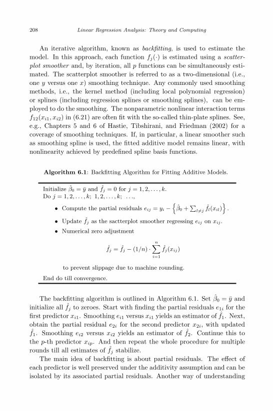
April 29, 2009 11:50 World Scientific Book - 9in x 6in Regression˙master
208 Linear Regression Analysis: Theory and Computing
An iterative algorithm, known as backfitting, is used to estimate themodel. In this approach, each function fj(·) is estimated using a scatter-plot smoother and, by iteration, all p functions can be simultaneously esti-mated. The scatterplot smoother is referred to as a two-dimensional (i.e.,one y versus one x) smoothing technique. Any commonly used smoothingmethods, i.e., the kernel method (including local polynomial regression)or splines (including regression splines or smoothing splines), can be em-ployed to do the smoothing. The nonparametric nonlinear interaction termsf12(xi1, xi2) in (6.21) are often fit with the so-called thin-plate splines. See,e.g., Chapters 5 and 6 of Hastie, Tibshirani, and Friedman (2002) for acoverage of smoothing techniques. If, in particular, a linear smoother suchas smoothing spline is used, the fitted additive model remains linear, withnonlinearity achieved by predefined spline basis functions.
Algorithm 6.1: Backfitting Algorithm for Fitting Additive Models.
Initialize β0 = y and fj = 0 for j = 1, 2, . . . , k.Do j = 1, 2, . . . , k; 1, 2, . . . , k; . . .,
• Compute the partial residuals eij = yi −
β0 +∑
l6=j fl(xil)
.
• Update fj as the sactterplot smoother regressing eij on xij .
• Numerical zero adjustment
fj = fj − (1/n) ·n∑
i=1
fj(xij)
to prevent slippage due to machine rounding.
End do till convergence.
The backfitting algorithm is outlined in Algorithm 6.1. Set β0 = y andinitialize all fj to zeroes. Start with finding the partial residuals e1i for thefirst predictor xi1. Smoothing ei1 versus xi1 yields an estimator of f1. Next,obtain the partial residual e2i for the second predictor x2i, with updatedf1. Smoothing ei2 versus xi2 yields an estimator of f2. Continue this tothe p-th predictor xip. And then repeat the whole procedure for multiplerounds till all estimates of fj stabilize.
The main idea of backfitting is about partial residuals. The effect ofeach predictor is well preserved under the additivity assumption and can beisolated by its associated partial residuals. Another way of understanding

April 29, 2009 11:50 World Scientific Book - 9in x 6in Regression˙master
Model Diagnostics 209
the algorithm is that, if a linear smoother is used, backfitting is equivalentto a Gauss-Seidel algorithm for solving a linear system of equations. Inorder to solve for z in a linear system of equations Az = b, one mayproceed successively to solve each zj in the j-th equation with the currentguess of other z’s and repeat the process until convergence.
The estimated fj ’s help identify and characterize nonlinear covariateeffects. The smoothness of fj is controlled by some smoothing parame-ters, e.g., the bandwidth in kernel methods and the penalty in smoothingsplines. In practice, selection of the smoothing parameter is made either byspecifying the number of degrees of freedom or via minimum generalizedcross-validation (GCV). Recall that GCV is yet another model selectioncriterion obtained as an approximation to PRESS in Chapter 5. We shallfurther explore its use in Section 7.3.4.
The additive models provide a useful extension of linear models andmake them more flexible. With retained additivity, the resultant model fitcan be interpreted in the same way as in linear models. This techniqueis generalized by Hastie and Tibshirani (1986) and Hastie and Tibshirani(1990) to handle other typed of responses, in which case it is called a Gen-eralized Additive Model. A GAM assumes that the mean of the dependentvariable depends on an additive form of functions of predictors through alink function. GAM permits the probability distribution of the response tobe any member from the exponential family. Many widely used statisticalmodels belong to this general family class, including Gaussian models forcontinuous data, logistic models for binary data, and Poisson models forcount data. We shall study these models in Chapter 8.
Algorithm 6.2: alternating conditional expectation (ACE)
(i) Initialization: set vi = g(yi) = (yi − y)/sy.
(ii) Regressing vi on xij , apply the backfitting algorithm for additivemodels to estimate fj(·)’s.
(iii) Compute ui =∑
j fj(xij). Regressing ui on yi, update the esti-mate g(·) as a scatterplot smoother.
(iv) Obtain the updated vi = g(yi) values and standardize them suchthat vi ← (vi − v)/sv.
(v) Go back to Step (ii) and iterate till convergence.
In terms of implementation, additive models and generalized additive

May 7, 2009 10:22 World Scientific Book - 9in x 6in Regression˙master
210 Linear Regression Analysis: Theory and Computing
models can be fit with PROC GAM in SAS. Two R packages, gam andmgcv, are also available.
6.2.3 ACE and AVAS
In the same vein as additive models, Breiman and Friedman (1985) putforward the ACE (alternating conditional expectation) algorithm, whichseeks optimal nonparametric transformations of both the response and pre-dictors. The working model of ACE is
g(yi) = β0 +k∑
j=1
fj(xi1) + εi. (6.22)
Consider the simple regression setting when k = 1. ACE approachesthe problem by minimizing the squared-error loss
Eg(Y )− f(X)2.Note that for fixed g, the function f that minimizes the squared loss isf(X) = Eg(Y )|X, and conversely, for fixed f the function g that mini-mizes the squared loss is g(Y ) = Ef(X)|Y . This is the key idea of theACE algorithm: it alternates between computations of these two condi-tional expectations via smoothing until convergence. When both g and f
are zero functions, the squared error loss is perfectly minimized. To pre-vent the procedure from convergence to this trivial case, ACE standardizesg(Y ) so that varg(Y ) = 1 at each step. The ACE procedure is outlinedin Algorithm 6.2.
Algorithm 6.3: AVAS Modification to Step (3) in the ACE Algorithm
• Compute fj(xij)’s and obtain ui =∑
j fj(xij);
• Compute the squared residuals r2i = (vi − ui)
2.
• Estimate the variance function of g(Y ), V (·), as a scatterplotsmoother that regresses r2
i against ui.
• Update the estimate g(·) as the variance stabilizing transformation(see Ex. 6.2.4)
g(y) =
∫ y
0
1√V (u)
du.
ACE has a close connection to canonical correlation analysis. ACE basi-cally searches for transformations to maximize the correlation between the
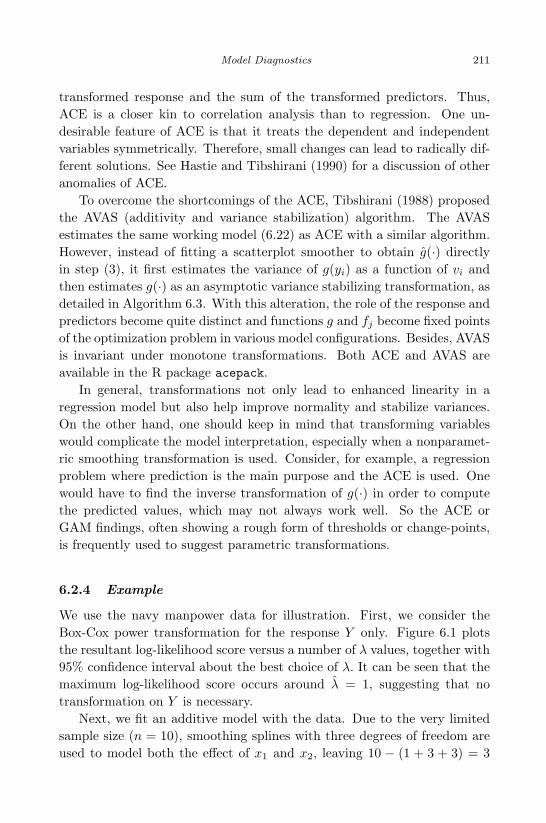
April 29, 2009 11:50 World Scientific Book - 9in x 6in Regression˙master
Model Diagnostics 211
transformed response and the sum of the transformed predictors. Thus,ACE is a closer kin to correlation analysis than to regression. One un-desirable feature of ACE is that it treats the dependent and independentvariables symmetrically. Therefore, small changes can lead to radically dif-ferent solutions. See Hastie and Tibshirani (1990) for a discussion of otheranomalies of ACE.
To overcome the shortcomings of the ACE, Tibshirani (1988) proposedthe AVAS (additivity and variance stabilization) algorithm. The AVASestimates the same working model (6.22) as ACE with a similar algorithm.However, instead of fitting a scatterplot smoother to obtain g(·) directlyin step (3), it first estimates the variance of g(yi) as a function of vi andthen estimates g(·) as an asymptotic variance stabilizing transformation, asdetailed in Algorithm 6.3. With this alteration, the role of the response andpredictors become quite distinct and functions g and fj become fixed pointsof the optimization problem in various model configurations. Besides, AVASis invariant under monotone transformations. Both ACE and AVAS areavailable in the R package acepack.
In general, transformations not only lead to enhanced linearity in aregression model but also help improve normality and stabilize variances.On the other hand, one should keep in mind that transforming variableswould complicate the model interpretation, especially when a nonparamet-ric smoothing transformation is used. Consider, for example, a regressionproblem where prediction is the main purpose and the ACE is used. Onewould have to find the inverse transformation of g(·) in order to computethe predicted values, which may not always work well. So the ACE orGAM findings, often showing a rough form of thresholds or change-points,is frequently used to suggest parametric transformations.
6.2.4 Example
We use the navy manpower data for illustration. First, we consider theBox-Cox power transformation for the response Y only. Figure 6.1 plotsthe resultant log-likelihood score versus a number of λ values, together with95% confidence interval about the best choice of λ. It can be seen that themaximum log-likelihood score occurs around λ = 1, suggesting that notransformation on Y is necessary.
Next, we fit an additive model with the data. Due to the very limitedsample size (n = 10), smoothing splines with three degrees of freedom areused to model both the effect of x1 and x2, leaving 10 − (1 + 3 + 3) = 3
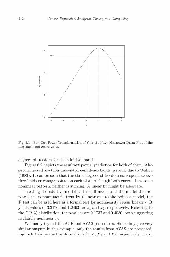
April 29, 2009 11:50 World Scientific Book - 9in x 6in Regression˙master
212 Linear Regression Analysis: Theory and Computing
−3 −2 −1 0 1 2 3
−10
−50
5
λ
log−
Like
lihoo
d
95%
Fig. 6.1 Box-Cox Power Transformation of Y in the Navy Manpower Data: Plot of theLog-likelihood Score vs. λ.
degrees of freedom for the additive model.Figure 6.2 depicts the resultant partial prediction for both of them. Also
superimposed are their associated confidence bands, a result due to Wahba(1983). It can be seen that the three degrees of freedom correspond to twothresholds or change points on each plot. Although both curves show somenonlinear pattern, neither is striking. A linear fit might be adequate.
Treating the additive model as the full model and the model that re-places the nonparametric term by a linear one as the reduced model, theF test can be used here as a formal test for nonlinearity versus linearity. Ityields values of 3.3176 and 1.2493 for x1 and x2, respectively. Referring tothe F (2, 3) distribution, the p-values are 0.1737 and 0.4030, both suggestingnegligible nonlinearity.
We finally try out the ACE and AVAS procedures. Since they give verysimilar outputs in this example, only the results from AVAS are presented.Figure 6.3 shows the transformations for Y , X1 and X2, respectively. It can
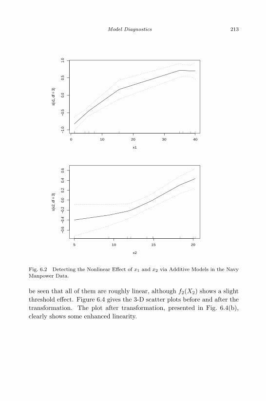
April 29, 2009 11:50 World Scientific Book - 9in x 6in Regression˙master
Model Diagnostics 213
0 10 20 30 40
−1.0
−0.5
0.0
0.5
1.0
x1
s(x1
, df =
3)
5 10 15 20
−0.6
−0.4
−0.2
0.0
0.2
0.4
0.6
x2
s(x2
, df =
3)
Fig. 6.2 Detecting the Nonlinear Effect of x1 and x2 via Additive Models in the NavyManpower Data.
be seen that all of them are roughly linear, although f2(X2) shows a slightthreshold effect. Figure 6.4 gives the 3-D scatter plots before and after thetransformation. The plot after transformation, presented in Fig. 6.4(b),clearly shows some enhanced linearity.

April 29, 2009 11:50 World Scientific Book - 9in x 6in Regression˙master
214 Linear Regression Analysis: Theory and Computing
1.0 1.5 2.0 2.5 3.0
−1.
0−
0.5
0.0
0.5
1.0
1.5
(a)
y
g(y)
0 10 20 30 40
−0.
50.
00.
51.
0
(b)
x1
f1(x
1)
5 10 15 20
−0.
6−
0.4
−0.
20.
00.
20.
4
(c)
x2
f2(x
2)
Fig. 6.3 AVAS Results for the Navy Manpower Data: (a) Plot of g(Y ); (b) Plot off1(X1); (c) Plot of f2(X2).
Problems
1. Let y(λ) be the response vector after applying a Box-Cox power trans-formation with λ. Assuming that y(λ) is normally distributed withmean Xβ and variance-covariance σ2I, show that the maximized log-likelihood score is given as in (6.15).
2. Given that variable W has mean u and variance V (u), show, using the
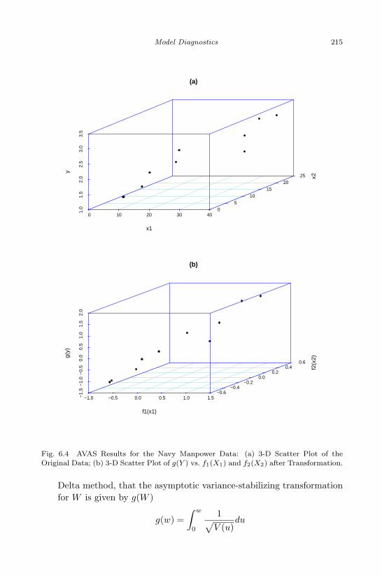
April 29, 2009 11:50 World Scientific Book - 9in x 6in Regression˙master
Model Diagnostics 215
(a)
0 10 20 30 40
1.0
1.5
2.0
2.5
3.0
3.5
0 5
1015
2025
x1
x2
y
(b)
−1.0 −0.5 0.0 0.5 1.0 1.5−1
.5−
1.0
−0
.5 0
.0 0
.5 1
.0 1
.5 2
.0
−0.6−0.4
−0.2 0.0
0.2 0.4
0.6
f1(x1)
f2(x
2)g(y
)
Fig. 6.4 AVAS Results for the Navy Manpower Data: (a) 3-D Scatter Plot of theOriginal Data; (b) 3-D Scatter Plot of g(Y ) vs. f1(X1) and f2(X2) after Transformation.
Delta method, that the asymptotic variance-stabilizing transformationfor W is given by g(W )
g(w) =∫ w
0
1√V (u)
du
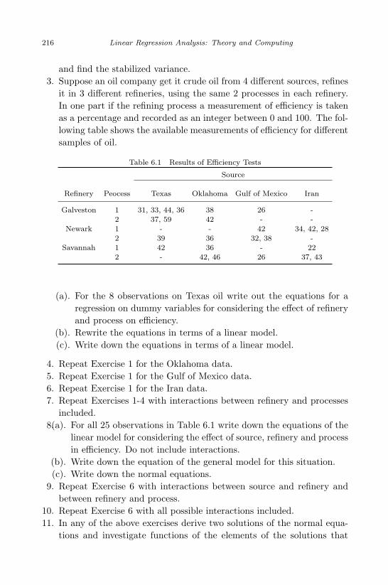
April 29, 2009 11:50 World Scientific Book - 9in x 6in Regression˙master
216 Linear Regression Analysis: Theory and Computing
and find the stabilized variance.3. Suppose an oil company get it crude oil from 4 different sources, refines
it in 3 different refineries, using the same 2 processes in each refinery.In one part if the refining process a measurement of efficiency is takenas a percentage and recorded as an integer between 0 and 100. The fol-lowing table shows the available measurements of efficiency for differentsamples of oil.
Table 6.1 Results of Efficiency Tests
Source
Refinery Peocess Texas Oklahoma Gulf of Mexico Iran
Galveston 1 31, 33, 44, 36 38 26 -2 37, 59 42 - -
Newark 1 - - 42 34, 42, 282 39 36 32, 38 -
Savannah 1 42 36 - 222 - 42, 46 26 37, 43
(a). For the 8 observations on Texas oil write out the equations for aregression on dummy variables for considering the effect of refineryand process on efficiency.
(b). Rewrite the equations in terms of a linear model.(c). Write down the equations in terms of a linear model.
4. Repeat Exercise 1 for the Oklahoma data.5. Repeat Exercise 1 for the Gulf of Mexico data.6. Repeat Exercise 1 for the Iran data.7. Repeat Exercises 1-4 with interactions between refinery and processes
included.8.(a). For all 25 observations in Table 6.1 write down the equations of the
linear model for considering the effect of source, refinery and processin efficiency. Do not include interactions.
(b). Write down the equation of the general model for this situation.(c). Write down the normal equations.
9. Repeat Exercise 6 with interactions between source and refinery andbetween refinery and process.
10. Repeat Exercise 6 with all possible interactions included.11. In any of the above exercises derive two solutions of the normal equa-
tions and investigate functions of the elements of the solutions that

April 29, 2009 11:50 World Scientific Book - 9in x 6in Regression˙master
Model Diagnostics 217
might be invariant to whatever solution is used.12. Repeat the above exercises assuming that processes are nested within
refineries, suitably modifying the interaction where necessary.

April 29, 2009 11:50 World Scientific Book - 9in x 6in Regression˙master
This page intentionally left blankThis page intentionally left blank

April 29, 2009 11:50 World Scientific Book - 9in x 6in Regression˙master
Chapter 7
Extensions of Least Squares
In this chapter, we study four extended uses of least squares for dealingwith a variety of regression problems often encountered in practice. Thefirst section deals with non-full rank linear models in which the designmatrix is not of full column rank. The generalized least squares (GLS)method is then introduced in Section 2. The GLS is useful for handlingcorrelated observations or nonconstant variances. In Section 3, we discussthe ridge regression and the least absolute shrinkage and selection operator(LASSO) proposed by Tibshirani (1996). Both are shrinkage estimators.The ridge regression is a remedial measure taken to handle severe multi-collinearity problems while the LASSO is particularly useful for variableselection. Finally, parametric nonlinear regression, where numerical meth-ods are necessary for solving the optimization with least squares, is brieflycovered in Section 4.
7.1 Non-Full-Rank Linear Regression Models
We first consider linear models with a non-full-rank design matrix X. Themodel specification is given as y = Xβ + ε, where X is n× (k + 1) of rankp < (k + 1) and ε ∼ (0, σ2I). Non-full-rank linear models often emerge indealing with data from analysis-of-variance (ANOVA) designs.
Example Consider, for instance, the One-Way ANOVA setting, whichcompares several population means due to different treatments received.This is essentially a regression problem that involves one continuous re-sponse Y and a categorial predictor Z. Suppose Z has c levels. With theregression approach, (c − 1) dummy or indicator variables are defined inorder to adequately and necessarily account for the c levels of Z. Inclusion
219

April 29, 2009 11:50 World Scientific Book - 9in x 6in Regression˙master
220 Linear Regression Analysis: Theory and Computing
Table 7.1 Layouts for Data Collected in One-way ANOVA Experiments.
(a) ANOVA Data Layout
category
1 2 · · · c
Y11 Y21 · · · Yc1
Y12 Y22 · · · Yc2
..
....
..
.
... Y2n2 · · ·...
.
.. Ycnc
Y1n1
(b) Regression Data Layout
Dummy Variables
subject Y Z Z1 Z1 · · · Zc
1 Y11 −→ Y1 1 1 0 · · · 0
..
....
..
....
..
....
..
.
n1 Y1n1 −→ Yn1 1 1 0 · · · 0
n1 + 1 Y21 −→ Yn1+1 2 0 1 · · · 0
......
......
......
...
n1 + n2 Y2n2 −→ Yn1+n2 2 0 1 · · · 0
..
....
..
....
..
....
..
.
n Ycnc −→ Yn c 0 0 · · · 1
of the (c − 1) dummy variables into the linear model results in a full-rankdesign matrix X and the estimation can be proceeded with ordinary leastsquares as usual.
On the other hand, one may alternatively define c indicator variablesZ1, Z2, . . . , Zc, one for each level, such that
Zij =
1, if the i-th subject is in the j-th catgory;0, otherwise
(7.1)
for j = 1, . . . , c and i = 1, . . . , n and then consider model
Yi = β0 + β1Zi1 + · · ·+ βcZic + εi,
= β0 + βj + εi, if the i-th subject falls into the j-th category,(7.2)
for i = 1, . . . , n. This model has the equivalent form to the classical one-wayANOVA model given by
Yij = µ + αj + εij (7.3)
for j = 1, . . . , ni and i = 1, . . . , c with correspondences µ = β0, αj = βj ,and n = n1 + n2 + . . . + nc.
To better see the correspondences, it is instructive to take a look at thedifferent data layouts for ANOVA and regression analysis, as illustrated inTable 7.1. Data for one-way ANOVA involve several independent randomsamples. The data originally collected arrive in with the layout shown inTable 7.1(a). In the study, ni individuals are randomly assigned to the i-thtreatment category for i = 1, . . . , c. When ni are all the same, the design is

April 29, 2009 11:50 World Scientific Book - 9in x 6in Regression˙master
Extensions of Least Squares 221
said to be balanced ; otherwise, it is an unbalanced design. Let Yij denotethe response value on j-th observation assigned to the i-th treatment orcategory. To prepare data for the regression approach, we put all responsevalues Yij ’s into one column and relabel the data as shown in Table 7.1(b).Also displayed in the table is the categorical variable Z which indicates theassignment of treatment, as well as the c dummy variables induced by Z.
Models (7.3) and (7.2) have very easy interpretation. Consider thebalanced design for example. With side condition
∑j αj = 0, µ =
∑µi/c
corresponds to the overall mean and αj = µj − µ is the difference betweenthe j-th treatment mean and the overall mean, measuring the effect of thej-th treatment. With model (7.2), the n× (c + 1) design matrix X is givenby
X =
1 1 0 · · · 0...
......
...1 1 0 · · · 01 0 1 · · · 0...
......
...1 0 1 · · · 0...
......
...1 0 0 · · · 1...
......
...1 0 0 · · · 1
, (7.4)
which is of rank c as adding the last c columns gives the first column j. ¶For non-full rank models, the matrix XtX is no longer non-singular
or invertible. Thus the ordinary LSE β = (XtX)−1Xty is not directlyapplicable. There are a few ways to get around this problem. We shallfocus on the one that utilizes the generalized inverse of XtX.
7.1.1 Generalized Inverse
We first give the definition of the generalized inverse and outline some ofits general properties.
Definition 7.1. Given an n × m matrix X, a generalized inverse of X,denoted by X−, is an m× n matrix such that XX−X = X.

April 29, 2009 11:50 World Scientific Book - 9in x 6in Regression˙master
222 Linear Regression Analysis: Theory and Computing
The following theorem establishes the existence of generalized inverses.
Theorem 7.1. Any matrix has a generalized inverse.
Proof. Consider an n×m matrix X of rank p. Let A be an n×p matrixwhose columns are a maximal set of linearly independent columns of X.Then every column of X can be expressed as a linear combination of A.
Thus X = AB for some p ×m matrix B which consists of the coefficientsfor these linear combinations. Since rank(AB) ≤ minrank(A), rank(B),it follows that both A and B are of rank p.
Since A is of full column rank, AtA must be positive definite. This canbe easily verified by considering quadratic form atAtAa = (Aa)tAa ≥ 0for any nonzero vector a. Moreover, Aa = 0 implies a = 0 as the columnsof A are linear independent. So atAtAa = (Aa)tAa > 0. Similarly, sinceB is of full row rank, BBt must be positive definite.
RewriteX = AB = ABBt(BBt)−1(AtA)−1AtAB = XBt(BBt)−1(AtA)−1AtX.
In other words, matrix A− = Bt(BBt)−1(AtA)−1At is a generalized in-verse of X. ¤A generalized inverse is not unique unless X is square and nonsingular,in which case X− = X−1. On the other hand, it can be made unique byimposing additional constraints. For example, the unique Moore-Penrosegeneralized inverse matrix of X satisfies that XX−X = X, X−XX− = X−,(XX−)t = X−X, and (X−X)t = XX−.
The following theorem provides important basis for inferences in non-full-rank models. We start with two useful lemmas.
Lemma 7.1. Given an n×m matrix X of rank p,
(i) XP = O for some matrix P if and only if XtXP = O.
(ii) X = X(XtX)−XtX and Xt = (XtX)−(XtX)Xt.
Proof.
(i) Let X = AB where A is n × p of rank p and B is p × m of rank p.Matrix A has linearly independent columns while matrix B has linearlyindependent rows. So both AA and BBt are invertible. It follows that
XtXP = O ⇐⇒ (AB)t(AB)P = BtAtABP = O
⇐⇒ (BBt)(AtA)BP = O ⇐⇒ BP = O
⇐⇒ ABP = XP = O.

April 29, 2009 11:50 World Scientific Book - 9in x 6in Regression˙master
Extensions of Least Squares 223
(ii) Consider (XtX)(XtX)−(XtX) = XtX by the definition of (XtX)−,
which can be rewritten as (XtX)(XtX)−(XtX)− I = O. Thus, bypart (1) of the lemma, X(XtX)−(XtX)− I = O. The desired resultsfollow. ¤
Theorem 7.2. Given an n×m matrix X of rank p, let
V = C(X) = µ ∈ Rn : µ = Xb for some vector b in Rm (7.5)
denote the column space of X. The projection matrix of V is given by
PV = X(XtX)−Xt (7.6)
for any generalized inverse of XtX. It follows that the matrix X(XtX)−Xt
remains invariant with any choice of (XtX)−.
Proof. To show X(XtX)−Xty is the projection of y on V for any giveny ∈ Rn, one needs to verify two conditions:
(i) X(XtX)−Xty ∈ V, which is obvious as
X(XtX)−Xty = X(XtX)−Xty = Xb.
(ii) y −X(XtX)−Xty ⊥ V. This is because, for any v ∈ V, v = Xb forsome b by the definition of V. We have
y −X(XtX)−XtytXb = 0
using (ii) of Lemma 7.1.
The invariance of X(XtX)−Xt with respect to the choices of (XtX)− isdue to the uniqueness of projection matrix. ¤
7.1.2 Statistical Inference on Null-Full-Rank Regression
Models
With the least squares criterion, we seek β that minimizes
Q(β) =‖ y −Xβ ‖2 .
Put in another way, we seek µ = Xβ that minimizes
Q(β) =‖ y − µ ‖2, for all µ ∈ V.
The mean vector µ is of form Xβ and hence must be in V. However,
Q(β) = ‖ y − µ ‖2= ‖ (y −PVy) + (PVy − µ) ‖2= ‖ y −PVy ‖2 + ‖ PVy − µ ‖2, since (y −PVy) ⊥ µ ∈ V≥ ‖ y −PVy ‖2 .
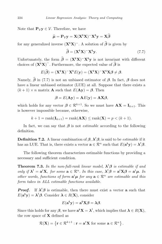
April 29, 2009 11:50 World Scientific Book - 9in x 6in Regression˙master
224 Linear Regression Analysis: Theory and Computing
Note that PVy ∈ V. Therefore, we have
µ = PVy = X(XtX)−Xty = Xβ
for any generalized inverse (XtX)−. A solution of β is given by
β = (XtX)−Xty. (7.7)
Unfortunately, the form β = (XtX)−Xty is not invariant with differentchoices of (XtX)−. Furthermore, the expected value of β is
E(β) = (XtX)−XtE(y) = (XtX)−XtXβ 6= β.
Namely, β in (7.7) is not an unbiased estimator of β. In fact, β does nothave a linear unbiased estimator (LUE) at all. Suppose that there exists a(k + 1)× n matrix A such that E(Ay) = β. Then
β = E(Ay) = AE(y) = AXβ,
which holds for any vector β ∈ Rk+1. So we must have AX = Ik+1. Thisis however impossible because, otherwise,
k + 1 = rank(Ik+1) = rank(AX) ≤ rank(X) = p < (k + 1).
In fact, we can say that β is not estimable according to the followingdefinition.
Definition 7.2. A linear combination of β, λtβ, is said to be estimable if ithas an LUE. That is, there exists a vector a ∈ Rn such that E(aty) = λtβ.
The following theorem characterizes estimable functions by providing anecessary and sufficient condition.
Theorem 7.3. In the non-full-rank linear model, λtβ is estimable if andonly if λt = atX, for some a ∈ Rn. In this case, λtβ = atXβ = atµ. Inother words, functions of form atµ for any a ∈ Rn are estimable and thisform takes in ALL estimable functions available.
Proof. If λtβ is estimable, then there must exist a vector a such thatE(aty) = λtβ. Consider λ ∈ R(X), consider
E(aty) = atXβ = λβ.
Since this holds for any β, we have atX = λt, which implies that λ ∈ R(X),the row space of X defined as
R(X) =r ∈ Rk+1 : r = atX for some a ∈ Rn
.

April 29, 2009 11:50 World Scientific Book - 9in x 6in Regression˙master
Extensions of Least Squares 225
On the other hand, if atX = λt for some vector a, then
EatX(XtX)−Xty = atX(XtX)−XtE(y)
= atX(XtX)−XtX
β
= atXβ using Lemma 7.1(ii),
= λtβ
Namely, λtβ has an LUE. ¤
A set of estimable functions λt1β, λt
2β, . . ., λtmβ, is said to be linearly
independent if the vectors λ1, . . . , λm are linearly independent. From theabove theorem, λi ∈ R(X). In addition, every row of Xβ must be estimable.Thus the following corollary becomes obvious.
Corollary 7.1. The maximum number of linearly independent estimablefunctions of β is p, the rank of X.
The next question is how to come up with a best linear unbiased esti-mator (BLUE) for an estimable function λtβ = atµ. This question is nicelyaddressed by the following Guass-Markov theorem. It turns out that thesolution can simply be obtained by plugging β or µ = Xβ.
Theorem 7.4. (Gauss-Markov) atµ is the BLUE of atµ.
Proof. First
atµ = atPVy = atX(XtX)−Xty
is linearly in y. Also, since µ ∈ V and hence PVµ = µ, it follows that
E(atµ) = atPVE(y) = atPVµ = atµ.
Therefore, atµ is an LUE of atµ.
Furthermore,
Var(atµ) = Var(atPVy) = σ2atPVPtVa
= σ2atPVa = σ2 ‖ PVa ‖2,since the projection matrix PV is idempotent. Suppose bty is any otherLUE of atµ. It follows from its unbiasedness that
E(bty) = btµ = atµ
⇐⇒ 〈a− b, µ〉 = 0 for any µ ∈ V;
⇐⇒ (a− b) ∈ V⊥⇐⇒ PV(a− b) = 0 or PVa = PVb.

April 29, 2009 11:50 World Scientific Book - 9in x 6in Regression˙master
226 Linear Regression Analysis: Theory and Computing
Consider
Var(bty) = σ2btb = σ2 ‖ b ‖2= σ2 ‖ b−PVb ‖2 +σ2 ‖ PVb ‖2= σ2 ‖ b−PVb ‖2 +σ2 ‖ PVa ‖2≥ σ2 ‖ PVa ‖2= Var(atµ),
with “=” held if and only if b = PVb = PVa, in which case bty = atPVy =atµ. Therefore, atµ is the BLUE. ¤
The following corollary gives the BLUE of λtβ.
Corollary 7.2. If λtβ is estimable, then λtβ = λ(XtX)−Xty, for anygeneralized inverse (XtX)−, is the BLUE.
Most theories in linear models can be justified using either properties ofmultivariate normal distributions or arguments from subspace and projects.The latter approach offers attractive geometric interpretations. We havefollowed this route to prove the Gauss-Markov (GM) theorem. It is clearthat the arguments in the proof apply with entirety to the full-rank linearmodels. The key point about the GM theorem is that, in order for atµ
to be the BLUE of atµ, µ needs to be the projection of y on V = C(X).Whether or not X is of full column rank only affects the way of computingthe projection matrix.
The sum of squared error (SSE) in non-full-rank models can be analo-gously defined:
SSE = (y −Xβ)t(y −Xβ) = yty − βtXty
= ‖ y −PVy ‖2=‖ PV⊥y ‖2= ytPV⊥y, (7.8)
which is invariant with different choices of β. It is easy to check thattrace(PV⊥) = n − rank(X) = n − p and hence E(SSE) = (n − p) · σ2
using the fact that
E(ytAy) = trace(AΣ) + µtAµ
for y ∼ (µ,Σ). A natural unbiased estimator of σ2 is given by
σ2 =SSE
n− p. (7.9)
It is important to note that we have not used the normality assumptionin any of the steps so far. In other words, all the above results hold withoutthe normality assumption.

April 29, 2009 11:50 World Scientific Book - 9in x 6in Regression˙master
Extensions of Least Squares 227
Example We continue with the earlier one-way ANOVA example. It canbe found that
XtX =
n n1 n2 · · · nc
n1 n1 0 · · · 0n2 0 n2 · · · 0...
......
...nc 0 0 · · · nc
(7.10)
and
Xty =
c∑
i=1
ni∑
j=1
yij ,
n1∑
j=1
y1j , . . . ,
nc∑
j=1
ycj
t
. (7.11)
A generalized inverse of XtX is given by
(XtX)− =
0 0 0 · · · 00 1/n1 0 · · · 00 0 1/n2 · · · 0...
......
...0 0 0 · · · 1/nc
. (7.12)
With this generalized inverse, it can be found that
β = (XtX)−Xty = (0, y1, y2, . . . , yc)t (7.13)
and
µ = Xβ = (y1, . . . , y1, y2, . . . , y2, . . . , yc, . . . , yc)t. (7.14)
There are other choices for (XtX)−, which yield different forms of β. Nev-ertheless, the predicted mean vector µ would remain the same. ¤
Now we add the normality assumption so that the non-full-rank model isspecified as
y ∼ N (Xβ, σ2I
), where X is n× (k + 1) of rank p. (7.15)
It follows immediately that
λtβ ∼ N λtβ, σ2 · λt(XtX)−λ
(7.16)
for any estimable linear function λtβ, since
Cov(λtβ) = Cov(λt(XtX)−Xty) = σ2λt(XtX)−XtX(XtX)−λ
= σ2atX(XtX)−XtX(XtX)−λ, plugging in λt = atX
= σ2 · atX(XtX)−λ, using Lemma 7.1(ii)
= σ2 · λt(XtX)−λ.

April 29, 2009 11:50 World Scientific Book - 9in x 6in Regression˙master
228 Linear Regression Analysis: Theory and Computing
Also,(n− p) · σ2
σ2=
SSE
σ2∼ χ2(n− p). (7.17)
Furthermore, it can be verified that SSE =‖ PV⊥y ‖2 is independent ofµ = PVy (and hence λtβ), using the fact that PVy and PV⊥y jointlyfollow a multivariate normal distribution with
Cov(PVy,PV⊥y) = σ2PVPtV⊥ = O.
Putting (7.16), (7.17), and their independence together yields
t =
(λtβ − λtβ)√σ2 · λt(XtX)−λ√
SSE/σ2
n− p
=(λtβ − λtβ)√σ2 · λt(XtX)−λ
∼ t(n− p) (7.18)
according to the definition of the central t distribution. This fact can beused to construct confidence intervals or conduct hypothesis testings forλtβ. For example, a (1− α)× 100% CI for an estimable λtβ is given by
λtβ ± t(n−p)1−α/2
√σ2 · λt(XtX)−λ. (7.19)
More generally, let Λ be an m × (k + 1) matrix with rows λti for
i = 1, . . . , m. Λβ is said to be estimable if every of its components, λtiβ, is
estimable. Furthermore, we assume that Λβ is a set of m linearly indepen-dent estimable functions, in which case Λ is of full row rank m. Under thisassumption, it can be verified that matrix Λ(XtX)−Λt is invertible (SeeProblem 0c). Following the same arguments as above, we have
Λβ ∼ N Λβ, σ2 ·Λ(XtX)−Λt
and hence
(Λβ −Λβ)t[Λ(XtX)−Λt
]−1(Λβ −Λβ)
σ2∼ χ2(m), (7.20)
which is independent of SSE/σ2 ∼ χ2(n− p). Therefore, according to thedefinition of F distribution,
F =(Λβ −Λβ)t
[Λ(XtX)−Λt
]−1(Λβ −Λβ)/(σ2 ·m)
SSE/(σ2 · (n− p))
=(Λβ −Λβ)t
[Λ(XtX)−Λt
]−1(Λβ −Λβ)/m
SSE/(n− p)∼ F (m, n− p), (7.21)
a fact being useful for testing general linear hypothesis H0 : Λβ = b.

May 7, 2009 10:22 World Scientific Book - 9in x 6in Regression˙master
Extensions of Least Squares 229
7.2 Generalized Least Squares
In an ordinary linear regression model, the assumption Cov(ε) = σ2I im-plies that yi’s are independent sharing the same constant variance σ2. Wenow consider data in which the continuous responses are correlated or havediffering variances. The model can be stated in a more general form givenby
y = Xβ + ε with ε ∼ (0, σ2V), (7.22)
where X is n × (p + 1) of full rank (p + 1) and V is a known positivedefinite matrix. The notation ε ∼ (0, σ2V
)means that E(ε) = 0 and
Cov(ε) = σ2V.
Estimation of Model (7.22) can be generally proceeded in the followingway. By applying a transformation, we first establish a connection betweenmodel (7.22) and an ordinary linear regression model where random errorsare independent with constant variance. All the statistical inference asso-ciated with model (7.22) can then be made through available results withthe ordinary linear model.
Using spectral decomposition, it can be established that V is positivedefinite if and only if there exists a nonsingular matrix P such that V =PPt. In particular, V 1/2 satisfies this condition. Multiplying Model (7.22)by P−1 on both sides yields that
P−1y = P−1Xβ + P−1ε,
where
Cov(P−1ε) = P−1Cov(ε)(P−1)t
= P−1σ2V(P−1)t = σ2 ·P−1PPt(P−1)t
= σ2I.
Define u = P−1y, Z = P−1X, and e = P−1ε. Then Model (7.22) can bewritten as an ordinary linear model form
u = Zβ + e with e ∼ (0, σ2I), (7.23)
where the design matrix Z is n × (p + 1) also of full rank (p + 1). All theinferences with Model (7.22) can be first processed through Model (7.23)and then re-expressed in terms of quantities in (7.22).

April 29, 2009 11:50 World Scientific Book - 9in x 6in Regression˙master
230 Linear Regression Analysis: Theory and Computing
7.2.1 Estimation of (β, σ2)
First of all, the least squares criterion isQ(β) = (u− Zβ)t(u− Zβ)
= (y −Xβ)t(P−1)tP−1(y −Xβ)
= (y −Xβ)tV−1(y −Xβ) (7.24)According to Model (7.23), the least squares estimator (LSE)
β =(ZtZ
)−1Ztu
is the BLUE of β. Re-expressing it givesβ =
(P−1X)t(P−1X)
−1(P−1X)tP−1y
=Xt(Pt)−1P−1X
−1Xt(Pt)−1P−1y
=Xt(PPt)−1X
−1Xt(PPt)−1y
=XtV−1X
−1XtV−1y. (7.25)
The estimator of this form β =XtV−1X
−1XtV−1y is often termed
as the generalized least squares estimator (GLSE). At the same time, thevariance-covariance matrix of β can also be obtained via Model (7.23):
Cov(β) = σ2(ZtZ
)−1 = σ2(P−1X)tP−1X
−1
= σ2Xt
(PPt
)−1X
−1
= σ2(XtV−1X
)−1. (7.26)
Similarly, an unbiased estimator of σ2 is
σ2 =(u− Zβ)t(u− Zβ)
n− (p + 1)
=(V−1y −V−1Xβ)t(V−1y −V−1Xβ)
n− (p + 1)
=(y −Xβ)tV−1(y −Xβ)
n− (p + 1)(7.27)
Expanding the numerator and plugging (7.25) give
σ2 =yt
V−1 −V−1X(XtV−1X)−1XtV−1
y
n− (p + 1). (7.28)
Many other measures associated with the GLS model (7.22) can beextracted in a similar manner. For example, the project or hat matrix Hin GLS is
H = Z(ZtZ)−1Zt
= P−1X(XtV−1X)−1XtP−1
= V−1/2X(XtV−1X)−1XtV−1/2, if P = V1/2 is used. (7.29)

April 29, 2009 11:50 World Scientific Book - 9in x 6in Regression˙master
Extensions of Least Squares 231
7.2.2 Statistical Inference
In order to facilitate statistical inference, we add the normality assumptionso that ε ∼ N (
0, σ2V). Hence Model (7.22) becomes
u = Zβ + e with e ∼ N (0, σ2I
). (7.30)
Again this allows us to apply the established results directly and then con-vert back to the GLS model (7.22).
First of all, β and σ2 are independent with
β ∼ N β, σ2(XtV−1X)−1
, (7.31)
n− (p + 1) · σ2
σ2∼ χ2n− (p + 1). (7.32)
These distributional properties make available the statistical inference onan individual regression parameter βj and the variance parameter σ2. Forexample, one may make the following probability statement according to(7.32)
P
χ2α/2(n− p− 1) <
n− (p + 1) · σ2
σ2< χ2
1−α/2(n− p− 1)
= 1− α,
where χ2α/2(n−p−1) denotes the (α/2)-th percentile of the χ2 with (n−p−1)
df. It follows that a (1− α)× 100% CI for σ2 can be given byn− (p + 1) · σ2
χ21−α/2(n− p− 1)
,n− (p + 1) · σ2
χ2α/2(n− p− 1)
.
Consider testing a general linear hypothesis about β of form H0 : Λβ =b, where Λ is m× (p+1) of rank m < (p+1). Working with Model (7.30),the F test applies with test statistic given by
F =(Λβ − b)t
Λ(ZtZ)−1Λt
−1(Λβ − b) /m
σ2
=(Λβ − b)t
Λ(XtV−1X)−1Λt
−1(Λβ − b) /m
σ2,
using ZtZ = XtV−1X. The test statistic F is distributed as F (m,n− p−1, λ) with noncentrality parameter
λ =(Λβ − b)t
Λ(XtV−1X)−1Λt
−1(Λβ − b)
σ2,
which reduces to central F (m,n− p− 1) under H0.

May 7, 2009 10:22 World Scientific Book - 9in x 6in Regression˙master
232 Linear Regression Analysis: Theory and Computing
Under the normality assumption, estimation of (β, σ2) can alternativelybe done via maximum likelihood. The likelihood function would be
l(β, σ2) =1
(2π)n/2 |σ2V|1/2exp− (y −Xβ)t(σ2V)−1(y −Xβ)
2
=
1(2πσ2)n/2 |V|1/2
exp− (y −Xβ)tV−1(y −Xβ)
2σ2
,
since |σ2V| = (σ2)n|V|. Differentiation of the log-likelihood log l(β, σ2)with respect to β and σ2 leads to their MLEs
β = (XtV−1X)−1XtV−1y, (7.33)
σ2 =(y −Xβ)tV−1(y −Xβ)
n. (7.34)
7.2.3 Misspecification of the Error Variance Structure
Suppose that the true model underlying the data is y = Xβ + ε withε ∼ (0, σ2V) in (7.22), and one mistakenly fits ordinary linear model withconstant variance for the error terms. Let β
= (XtX)−1Xty denote the
resultant least squares estimator. We will compare it to the BLUE β =(XtV−1X)−1X′V−1y in (7.25) to investigate the effects of mis-specificationof the error variance structure.
First consider
E(β) = E
(XtX)−1Xty
= (XtX)−1XtE(y)
= (XtX)−1XtXβ
= β.
Namely, β
remains unbiased for β with misspecified error variance struc-ture. Next, consider
Cov(β) = Cov
(XtX)−1Xty
= (XtX)−1XtCov(y)X(XtX)−1
= σ2 · (XtX)−1XtVX(XtX)−1. (7.35)
Comparatively, Cov(β) = σ2(XtV−1X)−1 as in (7.26). Since β is theBLUE of β and β
is an LUE, we must have that matrix Cov(β
)−Cov(β)
is semi-positive definite (see Problem 7.4). As a result, the standard errorsof the components β
j in β
are typically larger than the standard errorsof the components βj in β, which may lead to statistical insignificance forimportant predictors. In model diagnostics, unusually large standard errorsare often recognized as signals of misspecified error variance structure suchas heteroscedasticity, although other model deficiencies could be the cause.
April 29, 2009 11:50 World Scientific Book - 9in x 6in Regression˙master
Extensions of Least Squares 233
7.2.4 Typical Error Variance Structures
In the section, we list and discuss several common structures for the errorvariance.
Weighted Least Squares
The first case is when V = diag(vi) is diagonal. Thus P−1 = diag(1/√
vi).The least squares criterion in (7.24) becomes
Q(β) =n∑
i=1
1vi
(yi − xt
iβ)2
.
The quantity 1/vi plays the role of weight for the i-th observation. Ac-cordingly, the resultant estimate of β is termed as a weighted least squares(WLS) estimate. The diagonal structure of V implies independent errorsyet with nonconstant variances, which renders WLS a useful remedial tech-nique for handling the heteroscedasticity problem.
Note that the weights 1/vi are inversely proportional to the variancesσ2vi. Thus, observations yi with larger variance receive less weight andhence have less influence on the analysis than observations with smallervariance. This weighting strategy intuitively makes sense because the moreprecise is yi (i.e., with smaller variance), the more information it providesabout E(yi), and therefore the more weight it should receive in fitting theregression function.
It is important to notice that we have assumed the weights are specifiedexplicitly, or known up to a proportionality constant. This assumption isnot entirely unrealistic. In situations when the response variable Yi itself isthe average of a unit containing mi individuals from a population, the unitsize mi can be naturally used as the weight, recalling that Var(Yi) is equalto the population variance divided by mi. In addition, the error variancessometimes vary with a predictor variable Xj in a systematic fashion. Therelation, for instance, could be Var(εi) = σ2 xij . Hence V = diag(xij). Theassociated weights are 1/xij .
On the other hand, the matrix V is usually unknown in practice. Theweights must be estimated by modeling the heteroscedasticity. One com-mon approach formulates the variance as a known function of predictorsor the expected response. See, e.g., Carroll and Ruppert (1988) for a de-tailed treatment. An iterative weighted least squares (IWLS) procedure canbe employed to get improved estimation. In this procedure, one initiallyestimates the weights from the data, and then obtain the WLS estimates
April 29, 2009 11:50 World Scientific Book - 9in x 6in Regression˙master
234 Linear Regression Analysis: Theory and Computing
of β. Based on the residuals, the weights are re-estimated and the WLSestimation is updated. The process is iterated until the WLS fit gets stable.
AR(1) Variance Structure
Variance structures from time series models can be employed to modeldata collected over time in longitudinal studies. Consider a multiple linearregression model with random errors that follow a first-order autoregressiveprocess:
yi = xtiβ + εi with εi = ρεi−1 + νi, (7.36)
where νi ∼ N (0, σ2) independently and −1 < ρ < 1.
To find out the matrix V, we first rewrite εi
εi = ρ · εi−1 + νi
= ρ · (ρεi−2 + νi−1) + νi
= νt + ρνi−1 + ρ2νi−2 + ρ3νi−3 + · · ·
=∞∑
s=0
ρsνi−s.
It follows that E(εi) =∑∞
s=0 ρsE(νi−s) = 0 and
Var(εi) =∞∑
s=0
ρ2sVar(νi−s) = σ2∞∑
s=0
ρ2s =σ2
1− ρ2. (7.37)
Furthermore, the general formula for the covariance between two observa-tions can be derived. Consider
Cov(εi, εi−1) = E(εiεi−1) = E (ρ εi−1 + νi) · εi−1= E
ρ ε2
i−1 + νiεi−1
= ρ · E(ε2
i−1)
= ρ ·Var(εi−1) = ρ · σ2
1− ρ2
Also, using εi = ρ · εi−1 + νi = ρ · (ρεi−2 + νi−1) + νi, it can be found that
Cov(εi, εi−2) = E(εiεi−2) = E [ρ · (ρεi−2 + νi−1) + νi · εi−2]
= ρ2 · σ2
1− ρ2.
In general, the covariance between error terms that are s steps apart is
Cov(εi, εi−s) = ρs σ2
1− ρ2. (7.38)
Thus, the correlation coefficient is
cov(εi, εi−s) = ρs,

April 29, 2009 11:50 World Scientific Book - 9in x 6in Regression˙master
Extensions of Least Squares 235
which indicates a smaller correlation for any two observations that are fur-ther apart.
From (7.37) and (7.38), we have
V =σ2
1− ρ2·
1 ρ ρ2 . . . ρn−1
ρ 1 ρ . . . ρn−2
ρ2 ρ 1 . . . ρn−3
......
......
ρn−1 ρn−2 ρn−3 . . . 1
,
with inverse
V−1 =1σ2·
1 −ρ 0 . . . 0 0 0−ρ 1 + ρ2 −ρ . . . 0 0 00 −ρ 1 + ρ2 . . . 0 0 0...
......
......
...0 0 0 . . . −ρ 1 + ρ2 −ρ
0 0 0 . . . 0 −ρ 1
.
Note that ρ = 0 implies independent random errors. The Durbin-Watsontest (Durbin and Watson, 1951) for H0 : ρ = 0 is one of the few testsavailable for checking the independence assumption in linear regression.The test statistic is computed using the residuals from the ordinary leastsquares fit εi = yi − yi = yi − xt
iβ:
DW =∑n
i=2(εi − εi−1)2∑ni=1 ε2
i
. (7.39)
Durbin and Watson (1951) have also obtained the critical values of DW fordecision purposes.
Common Correlation
Another variance structure is
V =
1 ρ . . . ρ
ρ 1 . . . ρ...
......
ρ ρ . . . 1
,
in which all observations have the same variance and all pairs of them havethe same correlation ρ. This structure is appropriate in certain repeatedmeasures designs. Rewrite
V = (1− ρ)I + ρJ, (7.40)

April 29, 2009 11:50 World Scientific Book - 9in x 6in Regression˙master
236 Linear Regression Analysis: Theory and Computing
where J is the n× n matrix with all elements being 1. Its inverse is givenby
V−1 =1
1− ρ
(I− ρ
1 + (n− 1)ρJ)
.
It can be, very interestingly, shown (see, e.g., Rencher, 2000) that, withthe covariance structure in (7.40), the ordinary least squares estimates β
?=
(XtX)−1Xty turns out to be the BLUE of β.
7.2.5 Example
A data set is collected on 54 adult women in a study of the relationshipbetween diastolic blood pressure (DBP) and age. Fig. 7.1(a) gives a scat-ter plot of the data. There seems to be a very nice linear association,with greater variability are associated with larger DBO values though. Al-though transformations on the response or predictors may help stabilize thevariability, one might prefer the original form of DBP and age for betterinterpretation.
A simple linear regression model is first fit with ordinary least squares(OLS). The estimated coefficients are given in Panel (a) of Table 7.2.Fig. 7.1(b) plots the resultant residuals from OLS versus age. It can beseen that the variation increases dramatically with age, signaling heteroge-neous errors.
In order to apply the weighted least squares method, one must estimatethe weights. Common methods formulate the weights or the error varianceas a function of the predictors or the expected response. Alternatively, onemay group data in a way such that observations within the same groupshare a common variance.
Fig. 7.1 (c) and (d) plot |εi| and ε2i versus age, respectively. In order to
estimate weights, we regress the absolute value |εi| of residuals linearly onage. More specifically, the following steps are taken to obtain the WLS fit.
– Fit simple linear regression of |εi| versus age;– Obtain the fitted values, denoted by ri;– Compute weights as vi = 1/r2
i .
– Refit the linear model of DBP versus age with weights vi.
Panel (b) of Table 7.2 presents the resulting WLS fit, obtained from PROCREG with the WEIGHT statement. It can be seen that the LSE and WLSEare very close to each other. This is not surprising as both are unbiased

April 29, 2009 11:50 World Scientific Book - 9in x 6in Regression˙master
Extensions of Least Squares 237
20 30 40 50 60
7080
9010
011
0
(a)
age
dbp
20 30 40 50 60
−10
010
20
(b)
age
r
20 30 40 50 60
05
1015
20
(c)
age
|r|
20 30 40 50 60
010
020
030
040
0
(d)
age
squa
red
r
Fig. 7.1 (a) The Scatter Plot of DBP Versus Age; (b) Residual versus Age; (c) AbsoluteValues of Residuals |εi| Versus Age; (d) Squared Residuals ε2
i Versus Age.
estimates. However, the standard errors from WLS are considerably smallerthan those from OLS. As a result, estimates from WLS are statistically moresignificant.
One may repeat the above steps by iteratively updating the weights and

April 29, 2009 11:50 World Scientific Book - 9in x 6in Regression˙master
238 Linear Regression Analysis: Theory and Computing
Table 7.2 Analysis of the Diastolic Blood Pressure Data: (a) Ordinary LeastSquares (OLS) Estimates; (b) Weighted Least Squares (WLS) Fitting withWeights Derived from Regressing Absolute Values |εi| of the Residuals On Age.
(a) Parameter Estimates from OLS
Parameter Standard 95%Variable DF Estimate Error t Value Pr > |t| Confidence Limits
Intercept 1 56.15693 3.99367 14.06 <.0001 48.14304 64.17082age 1 0.58003 0.09695 5.98 <.0001 0.38548 0.77458
(b) WLS Estimates with Weights Derived from |εi|.
Parameter Standard 95%Variable DF Estimate Error t Value Pr > |t| Confidence Limits
Intercept 1 55.56577 2.52092 22.04 <.0001 50.50718 60.62436age 1 0.59634 0.07924 7.53 <.0001 0.43734 0.75534
the WLS fitting. Usually, convergence occurs after a couple of steps. Thisis because the updated weights are not very different from the initial onesdue to the unbiasedness or consistency of OLS estimates.
7.3 Ridge Regression and LASSO
Ridge regression is one of the remedial measures for handling severe mul-ticollinearity in least squares estimation. Multicollinearity occurs whenthe predictors included in the linear model are highly correlated with eachother. When this is the case, the matrix XtX tends to be singular or ill-conditioned and hence identifying the least squares estimates will encounternumerical problems.
To motivate the ridge estimator, we first take a look at the mean squarederror, MSE(b) = E ‖ b − β ‖2, of least squares estimator of β. MSE isa commonly-used measure for assessing quality of estimation, which canbreak into two parts: the squared bias plus the variance:
E ‖ b− β ‖2=∑
j
E(bj − βj)2 =∑
j
E(bj)− βj2 +∑
j
Var(bj). (7.41)
According to Gauss-Markov theorem, the least sqaures approach achievesthe smallest variance among all unbiased linear estimates. This howeverdoes not necessarily guarantee the minimum MSE. To better distinguish
April 29, 2009 11:50 World Scientific Book - 9in x 6in Regression˙master
Extensions of Least Squares 239
different types of estimators, let βLS
denote the ordinary least squares es-timator of β. Recall that E(β
LS) = β and Cov(β
LS) = σ2 · (XtX)−1. We
have
MSE(βLS
) = E ‖ βLS ‖2 − ‖ β ‖2
= trσ2(XtX)−1
= σ2 · tr
(XtX)−1
. (7.42)
Thus
E(‖ βLS ‖2) =‖ β ‖2 +σ2 · tr
(XtX)−1
. (7.43)
It can be seen that, with ill-conditioned XtX, the resultant LSE βLS
wouldbe large in length ‖ β
LS ‖ and associated with inflated standard errors.This inflated variation would lead to poor model prediction as well.
The ridge regression is a constrained version of least squares. It tack-les the estimation problem by producing biased estimator yet with smallvariances.
7.3.1 Ridge Shrinkage Estimator
For any estimator b, the least squares criterion can be rewritten as itsminimum, reached at β
LS, plus a quadratic form in b:
Q(b) = ‖ y −XβLS
+ XβLS −Xb ‖2
= (y −XβLS
)t(y −XβLS
) + (b− βLS
)tXtX(b− βLS
)
= Qmin + φ(b). (7.44)
Contours for each constant of the quadratic form φ(b) are hyper-ellipsoidscentered at the ordinary LSE β
LS. In view of (7.43), it is reasonable to
expect that, if one moves away from Qmin, the movement is in a directionwhich shortens the length of b.
The optimization problem in ridge regression can be stated as
minimizing ‖ β ‖2 subject to (β − βLS
)tXtX(β − βLS
) = φ0
for some constant φ0. The enforced constrain guarantees a relatively smallresidual sum of squares Q(β) when compared to its minimum Qmin.
Fig. 7.2(a) depicts the contours of residual sum of squares together with theL2 ridge constraint in the two-dimensional case. As a Lagrangian problem,it is equivalent to minimizing
Q?(β) =‖ β ‖2 +(1/k)
(β − βLS
)tXtX(β − βLS
)− φ0
,

April 29, 2009 11:50 World Scientific Book - 9in x 6in Regression˙master
240 Linear Regression Analysis: Theory and Computing
(a)
b2
b1
LSE
(b)
b2
b1
LSE
Fig. 7.2 Estimation in Constrained Least Squares in the Two-dimensional Case: Con-tours of the Residual Sum of Squares and the Constraint Functions in (a) Ridge Regres-sion; (b) LASSO.
where 1/k is the multiplier chosen to satisfy the constraint. Thus
∂Q?
∂β= 2β + (1/k)
2(XtX)β − 2(XtX)β
LS
= 0,
which yields the ridge estimator
βR
=XtX + kI
−1Xty. (7.45)

April 29, 2009 11:50 World Scientific Book - 9in x 6in Regression˙master
Extensions of Least Squares 241
An equivalent way is to write the ridge problem in the penalized orconstrained least squares form by
minimizing ‖ y −Xβ ‖2, subject to ‖ β ‖2≤ s, (7.46)
for some constant s. The Lagrangian problem becomes minimizing
‖ y −Xβ ‖2 +λ· ‖ β ‖2,which yields the same estimator given in (7.45). The penalty parameterλ ≥ 0 controls the amount of shrinkage in ‖ β ‖2. The larger value of λ,the greater amount of shrinkage. For this reason, the ridge estimator isalso called the shrinkage estimator. There is a one-to-one correspondenceamong λ, s, k, and φ0.
It is important to note that the ridge solution is not invariant underscaling of the inputs. Thus one should standardize both the inputs and theresponse
x′ij =xij − xj
sxj
and y′i =yi − y
sy
before computing the shrinkage estimator in (7.45). With the standardizedvariables, the matrices XtX and Xty become
XtX = RXX and Xty = rXY ,
where RXX denotes the correlation matrix among Xj ’s and rY X denotesthe correlation vector between Y and all Xj ’s. Hence the ridge estimatorbecomes
βR
= RXX + kI−1 rY X . (7.47)
In the case of orthogonal predictors where XtX = I, it can be easily seenthat the ridge estimates are just a scaled version of LSE, i.e., β
R= 1/(1 +
k)·βLSfor some constant shrinkage 0 ≤ 1/(1+k) ≤ 1. Besides, the intercept
β0 is automatically suppressed as 0 when working with standardized data.Given a ridge estimator β
R, one needs transform its components back
in order to get the fitted linear equation between the original Y and Xj
values. It is convenient to express in matrix form the normalization and itsinverse transformation involved. Let X0 be the original design matrix. Itscentered version is
Xc = (I− jnjtn/n)X0
and its normalized version is
X = XcL−1/2

April 29, 2009 11:50 World Scientific Book - 9in x 6in Regression˙master
242 Linear Regression Analysis: Theory and Computing
where jn is the n-dimensional vector with elements ones and L is a diagonalmatrix with diagonal elements from the matrix Xt
cXc, i.e.,
L = diag(Xt
cXc
).
Similarly, the original response vector y0 can be normalized as
y =(I− jnj′n/n)y0
sy,
where sy denotes the sample standard deviation of y0. Given the ridgeestimator β
Rin (7.45), suppose that we want to predict with a new data
matrix Xnew, which is m × p on the original data scale. Note that we donot need to add jm as the first column of Xnew as the intercept has beensuppressed. The predicted vector ynew is then given as
ynew = sy ·(
Xnew − jmjtnX/n)L−1/2β
R+ jmjtny/n
. (7.48)
Next, we shall compute the expectation and variance of βR. Eventually,
we want to compare βR
with βLS
to see whether a smaller MSE can beachieved by β
Rfor certain values of k. Denote
Z =I + k(XtX)−1
−1. (7.49)
Then
βR
= Z βLS
. (7.50)
It follows that
E(βR) = Zβ (7.51)
Cov(βR) = σ2 · Z(XtX)−1Zt. (7.52)
Let
λmax = λ1 ≥ λ2 ≥ · · · ≥ λm = λmin > 0 (7.53)
denote the eigenvalues of XtX, then the corresponding eigenvalues of Z areλj/(λj + k). From (7.42),
MSE(βLS
) = σ2 ·∑
j
1/λj (7.54)
For the components in ridge estimator, it can be found from (7.51) and(7.52) that the sum of their squared biases is
∑
j
E(βR
j )− βj
2
=
E(βR)− β
t E(β
R)− β
= βt(I− Z)t(I− Z)β
= k2βt(XtX + kI)−2, β using Problem 7.7.4.2,

April 29, 2009 11:50 World Scientific Book - 9in x 6in Regression˙master
Extensions of Least Squares 243
and the sum of their variances is
trCov(βR) = σ2 · tr
(XtX)−1ZtZ
= σ2∑
j
1λj· λ2
j
(λj + k)2
= σ2 ·∑
j
λj
(λj + k)2.
Therefore, the MSE for the ridge estimator is
MSE(βR, k) = σ2 ·
∑
j
λj
(λj + k)2+ k2βt(XtX + kI)−2β
= γ1(k) + γ2(k). (7.55)
The function γ1(k) is a monotonic decreasing function of k while γ2(k)is monotonically increasing. The constant k reflects the amount of biasincreased and the variance reduced. When k = 0, it becomes the LSE.Hoerl and Kennard (1970) showed that there always exists a k > 0 suchthat
MSE(βR, k) < MSE(β
R, 0) = MSE(β
LS).
In other words, the ridge estimator can outperform the LSE in terms ofproviding a smaller MSE. Nevertheless, in practice the choice of k is yet tobe determined and hence there is no guarantee that a smaller MSE alwaysbe attained by ridge regression.
7.3.2 Connection with PCA
The singular value decomposition (SVD) of the design matrix X can providefurther insights into the nature of ridge regression. We shall establish,following Hastie, Tibshirani, and Friedman (2002), a connection betweenridge regression and principal component analysis (PCA).
Assume the variables are standardized or centered so that the matrix
S = XtX/n (7.56)
gives either the sample variance-covariance matrix or the sample correlationmatrix among predictors Xj ’s. The SVD of the n× p design matrix X hasthe form
X = UDVt, (7.57)

May 7, 2009 10:22 World Scientific Book - 9in x 6in Regression˙master
244 Linear Regression Analysis: Theory and Computing
where U and V are n×p and p×p orthogonal matrices such that the columnsof U form an orthonormal basis of the column space of X and the columnsof V form an orthonormal basis of the row space of X; the p× p diagonalmatrix D = diag(dj) with diagonal entries dj , |d1| ≥ |d2| ≥ · · · ≥ |dp| beingthe singular values of X. It follows that
XtX = VD2Vt, (7.58)
which provides the spectral decomposition of XtX. Referring to (7.53), wehave the correspondence λj = d2
j . In addition, the spectral decompositionfor S in (7.56) would be
S = (1/n) ·VD2Vt, (7.59)
with eigenvalues d2j/n and eigenvectors vj (i.e., the j-th column of V).
We first briefly outline the main results of principal component analysis(PCA). A PCA is concerned with explaining the variance-covariance struc-ture through uncorrelated linear combinations of original variables. Weconsider the sample version of PCA. Let xi denote the i-th row in the cen-tered or standardized design matrix X for i = 1, . . . , n. It can be easily seenthat the n values qtx1,qtx2, . . . ,qtxn of any linear combination qtxi hassample variance qtSq. These n values are elements in vector Xq inducedby the direction q.
The problem of PCA can be formulated as follows. We seek the directionq1 subject to qt
1q1 = 1 such that values in Xq1, referred to the first sampleprincipal component, has the largest sample variance. Next, we seek thesecond sample principal component Xq2 with qt
2q2 = 1 such that its valueshave the largest sample variance and zero sample covariance with values ofthe first principal component. In general, at the j-th step for j = 1, . . . , p,
we seek the j-th principal component Xqj subject to qtjqj = 1 such that
its values have the largest sample variance and zero sample covariance withvalues in each of the preceding principal components. It turns out that theprincipal component directions are exactly provided by the eigenvectors ofS, i.e., qj = vj . The j-th principal component is Xvj , which has a samplevariance of d2
j/n. A small singular value d2j is associated with PC directions
having small variance. Since Xvj = dj ·uj according to (7.57), uj, the j-thcolumn of U, is the j-th normalized principal component. The proof anddetailed elaboration of PCA can be found in, e.g., Johnson and Wichern(2001).
Using the SVD of X in (7.57), the least squares fitted vector µLS can

April 29, 2009 11:50 World Scientific Book - 9in x 6in Regression˙master
Extensions of Least Squares 245
be rewritten as
µLS = XβLS
= X(XtX)−1Xty
= UDVt(VDtUtUDVt)−1VDtUty
= UDVt(VD−2Vt)−1VDtUty
= UDVtVD2VtVDtUty
= UUty
=p∑
j=1
(utjy) · uj (7.60)
Note that Uty or utjy’s are the coordinates of y with respect to the columns
of U. Recall that uj’s are the orthonormal basis spanning the column spaceof X and also the normalized sample principal components.
Another approach to deal with multicollinearity is called principal com-ponents regression (PCR). In this approach, y is regressed on the first m
principal components by rejecting the last (p−m) components that explaina relatively small portion of variation in X. Thus the fitted response vectorwould be
µPCR =m∑
j=1
(utjy) · uj . (7.61)
The implicit assumption is that the response tends to vary most in thedirections where the predictors have large variations.
The fitted vector based on ridge regression, after similar simplification,is
µR = XβR
= X(XtX + kI)−1Xty
= UD(D2 + kI)−1DUty
=p∑
j=1
d2j
d2j + k
(utjy) · uj . (7.62)
Thus, similar to least squares regression, the ridge solution computes thecoordinates of y with respect to the orthonormal basis U and then shrinksthem by the factor d2
j/(d2j + k). Note that d2
j/(d2j + k) ≤ 1 as k ≥ 0. With
this strategy, a greater amount of shrinkage is applied to basis vectors orprincipal component vectors corresponding to smaller d2
j = λj . Insteadof rejecting low-variance directions as in PCR, ridge regression keeps allprincipal component directions but weighs the coefficients by shrinking low-variance directions more.

April 29, 2009 11:50 World Scientific Book - 9in x 6in Regression˙master
246 Linear Regression Analysis: Theory and Computing
7.3.3 LASSO and Other Extensions
The LASSO or lasso (least absolute shrinkage and selection operator) isanother shrinkage method like ridge regression, yet with an important andattractive feature in variable selection.
To motivate, we continue with the comparison between ridge regressionand PCR from the variable selection perspective. PCR, same as subsetselection procedures, is a discrete selecting process - regressors or the prin-cipal components of them are either fully retained or completely droppedfrom the model. Comparatively, the ridge regression makes the selectionprocess continuous by varying shrinkage parameter k and hence is more sta-ble. On the other hand, since ridge regression does not set any coefficientsto 0, it does not give an easily interpretable model as in subset selection.The lasso technique is intended to balance off in between and retains thefavorable features of both subset selection and ridge regression by shrinkingsome coefficients and setting others to 0.
The lasso estimator of β is obtained by
minimizing ‖ y −Xβ ‖2, subject top∑
j=1
|βj | ≤ s. (7.63)
Namely, the L2 penalty∑
j β2j in ridge regression is replaced by the L1
penalty∑
j |βj | in lasso. If s is chosen greater than or equal to∑
j |βLSj |,
then the lasso estimates are the same as the LSE; if s is chosen to be smaller,then it will cause shrinkage of the solutions towards 0.
Fig. 7.2(b) portrays the lasso estimation problem in the two dimensionalcase. The constraint region in ridge regression has a disk shape while theconstraint region in lasso is a diamond. Both methods find the first pointat which the elliptical contours hit the constraint region. However, unlikethe disk, the diamond has corners. If the solution occurs at a corner, thenit has one coefficient βj equal to zero.
The lasso solution is generally competitive with ridge solution yet withmany zero coefficient estimates. Insight about the nature of the lasso canbe further gleaned from orthonormal designs where XtX = I. In this case,the lasso estimator can be shown to be
βlassoj = sign(βLS
j )|βLS
j | − γ
+, (7.64)
where γ is determined by the condition∑
j |βlassoj | = s. Thus, coefficients
less than the threshold γ would be automatically suppressed to 0 whilecoefficients larger than γ would be shrunk by a unit of γ. Hence, the lasso

May 7, 2009 10:22 World Scientific Book - 9in x 6in Regression˙master
Extensions of Least Squares 247
technique performs as a variable selection operator. By increasing s indiscrete steps, one obtains a sequence of regression coefficients where thosenonzero coefficients at each step correspond to selected predictors.
In general, the nonsmooth nature of the lasso constraint makes the so-lutions nonlinear in y. In the initial proposal of lasso by Tibshirani (1996),quadratic programming was employed to solve the optimization problemby using the fact that the condition
∑j |βj | ≤ s is equivalent to δt
iβ ≤ s
for all i = 1, 2, . . . , 2p, where δi is the p-tuples of form (±1,±1, . . . ,±1).Later, Osborne, Presnell, and Turlach (2000a, 2000b) developed a compactdescent method for solving the constrained lasso problem for any fixed s
and a “homotopy method” that completely describe the possible selectionregimes in the lasso solution. In the same vein, Efron et al. (2004) derived aparallel variant, called the least angle regression (LARS). LARS facilitatesa variable selection method in its own right. More importantly, the entirepath of lasso solutions as s varies from 0 to +∞ can be extracted with aslight modification on LARS.
The LARS method works with normalized data and iteratively builds upthe predicted response µ with updating steps, analogous to boosting (see,e.g., Freund and Schapire, 1997). The main steps of LARS are first brieflyoutlined, with some details following up. Initially all coefficients are set tozero. The predictor that has highest correlation with the current residual,which is the response itself in this stage, is identified. A step is then taken inthe direction of this predictor. The length of this step, which corresponds tothe coefficient for this predictor, is chosen such that some other predictor(i.e., the second predictor entering the model) and the current predictedresponse have the same correlation with the current residual. Next, thepredicted response moves in the direction that is equiangular between orequally correlated with these two predictors. Moving in this joint directionensures that these two predictors continue to have a common correlationwith the current residual. The predicted response moves in this directionuntil a third predictor has the same correlation with the current residualas the two predictors already in the model. A new joint direction that isequiangular between these three predictors is determined and the predictedresponse moves in this direction until a fourth predictor having the samecorrelation with the current residual joins the set. This process continuestill all predictors have entered the model.
More specifically, start with µ0 = 0. Let µA denote the current LARSestimate for the predicted vector, where A is the active set of indices cor-responding to predictors that have the great absolute correlations with the

April 29, 2009 11:50 World Scientific Book - 9in x 6in Regression˙master
248 Linear Regression Analysis: Theory and Computing
current residuals, i.e., predictors in the current model. The sample corre-lation between the residuals and values of each predictor indexed in A isgiven as
c = Xt(y − yA)
owing to normalization. Thus,
A = j : |cj | = C with C = maxj
(|cj |).
Let sj = sign(cj) for j ∈ A be the sign of the correlation between Xj in theactive set and the current residuals and let XA = (sjxj), for j ∈ A, be thedesign matrix containing all signed active predictors. Compute matrices
GA = XtAXA, (7.65)
AA = (jtAG−1A jA)−1/2, (7.66)
wA = AAG−1A jA, (7.67)
where jA is the vector of 1’s of dimension equal to |A|, the cardinality ofA. Then the equiangular vector
uA = XAwA with ‖ uA ‖= 1 (7.68)
makes equal angles, less than 90, with each column of XA, i.e.,
XtAuA = AAjA. (7.69)
Also compute the correlations between each predictor with the equiangularvector uA, given as
a = XtuA.
Then, the next updating step of the LARS algorithm is
µA+ = µA + γuA, (7.70)
where
γ = min+j∈Ac
C − cj
AA − aj,
C + cj
AA + aj
(7.71)
and the min+ means that the minimum is taken over only these positivecomponents. Let j be the minimizing index in (7.71). Then Xj is thevariable added to the active set and the new maximum absolute correlationbecomes C − γAA.
Two notable remarks are in order. First, LARS is rather thrifty incomputation, simply requiring a total of p steps. Secondly, surprisingly,with a slight modification of LARS, one can obtain a sequence of lasso

April 29, 2009 11:50 World Scientific Book - 9in x 6in Regression˙master
Extensions of Least Squares 249
estimates, from which all other lasso solutions can be obtained by linearinterpolation. The modification is that, if a non-zero coefficient turns intozero, it will be removed from the active set of predictors and the jointdirection will be recomputed.
Extensions and further explorations of LASSO are currently under in-tensive research. For example, the BRIDGE regression, introduced byFrank and Friedman (1993), generalizes the penalty term by applying aLq constraint with q ≥ 0. The optimization problem becomes
minimizing ‖ y −Xβ ‖2, subject to∑
|βj |q ≤ s, (7.72)
or equivalently,
minimizing ‖ y −Xβ ‖2 +λ ·∑
|βj |q.
The case when q = 0 corresponds to variable subset selection as the con-straint simply counts the number of nonzero parameters and hence penalizesfor model complexity; q = 1 corresponds to the lasso penalty and q = 2corresponds to the ridge regression; when q > 2, the constraint region be-comes a polyhedron with many corners, flat edges, and faces, and hence itis more likely to have zero-valued coefficients.
Table 7.3 The Macroeconomic Data Set in Longley (1967).
GNP.deflator GNP Unemployed Armed.Forces Population Year Employed
83.0 234.289 235.6 159.0 107.608 1947 60.32388.5 259.426 232.5 145.6 108.632 1948 61.12288.2 258.054 368.2 161.6 109.773 1949 60.17189.5 284.599 335.1 165.0 110.929 1950 61.18796.2 328.975 209.9 309.9 112.075 1951 63.22198.1 346.999 193.2 359.4 113.270 1952 63.63999.0 365.385 187.0 354.7 115.094 1953 64.989100.0 363.112 357.8 335.0 116.219 1954 63.761101.2 397.469 290.4 304.8 117.388 1955 66.019104.6 419.180 282.2 285.7 118.734 1956 67.857108.4 442.769 293.6 279.8 120.445 1957 68.169110.8 444.546 468.1 263.7 121.950 1958 66.513112.6 482.704 381.3 255.2 123.366 1959 68.655114.2 502.601 393.1 251.4 125.368 1960 69.564115.7 518.173 480.6 257.2 127.852 1961 69.331116.9 554.894 400.7 282.7 130.081 1962 70.551
mean 101.681 387.698 319.331 260.669 117.424 8.5? 65.317sd 10.792 99.395 93.446 69.592 6.956 4.761 3.512

April 29, 2009 11:50 World Scientific Book - 9in x 6in Regression˙master
250 Linear Regression Analysis: Theory and Computing
7.3.4 Example
Implementation of ridge regression is widely available, e.g., in PROC REGof SAS and the function lm.ridge in R (http://www.r-project.org/) pack-age MASS. LASSO is relatively new, available in the experimental SAS pro-cedure PROC GLMSELECT and in the R packages: lasso2 and lars.We shall discuss many practical issues involved in both ridge regressionand LASSO through a macroeconomic data set in Longley (1967), whichis a well-known example for highly collinear regression. The data set, asprovided in Table 7.3, contains n = 16 observations on seven economicalvariables, observed yearly from 1947 to 1962. The response variable isEmployed. A brief description of the data set is provided in Table 7.4.
Table 7.4 Variable Description for Longley’s (1967) Macroeconomic Data.
Variable Name Description
X1 GNP.deflator GNP implicit price deflator (1954=100)
X1 GNP Gross National Product.
X1 Unemployed number of unemployed.
X1 Armed.Forces number of people in the armed forces.
X1 Population “noninstitutionalized” population ≥ 14 years of age.
X1 Year the year (time).
Y1 Employed number of people employed.
To proceed, we first take the transformation Year = Year−1946 so thatthe time points are integers from 1 to 16 and then standardize or normalizeevery variable in the data set. Thus the intercept term is suppressed in allthe following models that we consider.
For exploratory data analysis (EDA) purposes, Fig. 7.3 gives a scatterplot for every pair of the variables. It can be seen that several predictorshave strong linear relationships with each other, as also evidenced by highcorrelation coefficients from the correlation matrix given in panel (a) ofTable 7.5. Indeed, the variance inflation factor (VIF) values, given in thelast column of panel (b) in Table 7.5, show that severe multicollinearityexists among all predictors except Armed.Forces (X4). Recall that theVIF is a commonly used indicator for multicollinearity and computed asthe coefficient of determination or R2 in the linear model that regressesXj on other predictors (X1, . . . , Xj−1, Xj+1, . . . , Xp) in the model, for j =1, . . . , p. It measures how large the variance of βLS
j is relative to its variancewhen predictors are uncorrelated. Usually a VIF value larger than 10, in

April 29, 2009 11:50 World Scientific Book - 9in x 6in Regression˙master
Extensions of Least Squares 251
GNP.deflator
−1.5 0.0 1.5 −1.5 0.0 1.0 −1.5 0.0 1.0
−1.5
−0.5
0.5
1.5
−1.5
−0.5
0.5
1.5
GNP
Unemployed
−1.5
−0.5
0.5
1.5
−1.5
−0.5
0.5
1.5
Armed.Forces
Population
−1.5
−0.5
0.5
1.5
−1.5
−0.5
0.5
1.5
Year
−1.5 0.0 1.0 −1.5 0.0 1.0 −1.5 0.0 1.5 −1.5 0.0 1.0
−1.5
−0.5
0.5
1.5
Employed
longley data
Fig. 7.3 Paired Scatter Plots for Longley’s (1967) Economic Data.
which case R2 > .90, causes concerns.The least squares estimation shows insignificance of both GNP and
Population. This contradicts the impression gained from the paired scat-ter plots. Applying the stepwise selection procedure leads to elimination
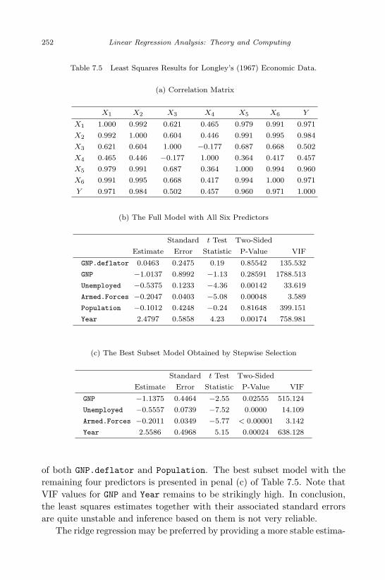
April 29, 2009 11:50 World Scientific Book - 9in x 6in Regression˙master
252 Linear Regression Analysis: Theory and Computing
Table 7.5 Least Squares Results for Longley’s (1967) Economic Data.
(a) Correlation Matrix
X1 X2 X3 X4 X5 X6 Y
X1 1.000 0.992 0.621 0.465 0.979 0.991 0.971
X2 0.992 1.000 0.604 0.446 0.991 0.995 0.984
X3 0.621 0.604 1.000 −0.177 0.687 0.668 0.502
X4 0.465 0.446 −0.177 1.000 0.364 0.417 0.457
X5 0.979 0.991 0.687 0.364 1.000 0.994 0.960
X6 0.991 0.995 0.668 0.417 0.994 1.000 0.971
Y 0.971 0.984 0.502 0.457 0.960 0.971 1.000
(b) The Full Model with All Six Predictors
Standard t Test Two-Sided
Estimate Error Statistic P-Value VIF
GNP.deflator 0.0463 0.2475 0.19 0.85542 135.532
GNP −1.0137 0.8992 −1.13 0.28591 1788.513
Unemployed −0.5375 0.1233 −4.36 0.00142 33.619
Armed.Forces −0.2047 0.0403 −5.08 0.00048 3.589
Population −0.1012 0.4248 −0.24 0.81648 399.151
Year 2.4797 0.5858 4.23 0.00174 758.981
(c) The Best Subset Model Obtained by Stepwise Selection
Standard t Test Two-Sided
Estimate Error Statistic P-Value VIF
GNP −1.1375 0.4464 −2.55 0.02555 515.124
Unemployed −0.5557 0.0739 −7.52 0.0000 14.109
Armed.Forces −0.2011 0.0349 −5.77 < 0.00001 3.142
Year 2.5586 0.4968 5.15 0.00024 638.128
of both GNP.deflator and Population. The best subset model with theremaining four predictors is presented in penal (c) of Table 7.5. Note thatVIF values for GNP and Year remains to be strikingly high. In conclusion,the least squares estimates together with their associated standard errorsare quite unstable and inference based on them is not very reliable.
The ridge regression may be preferred by providing a more stable estima-
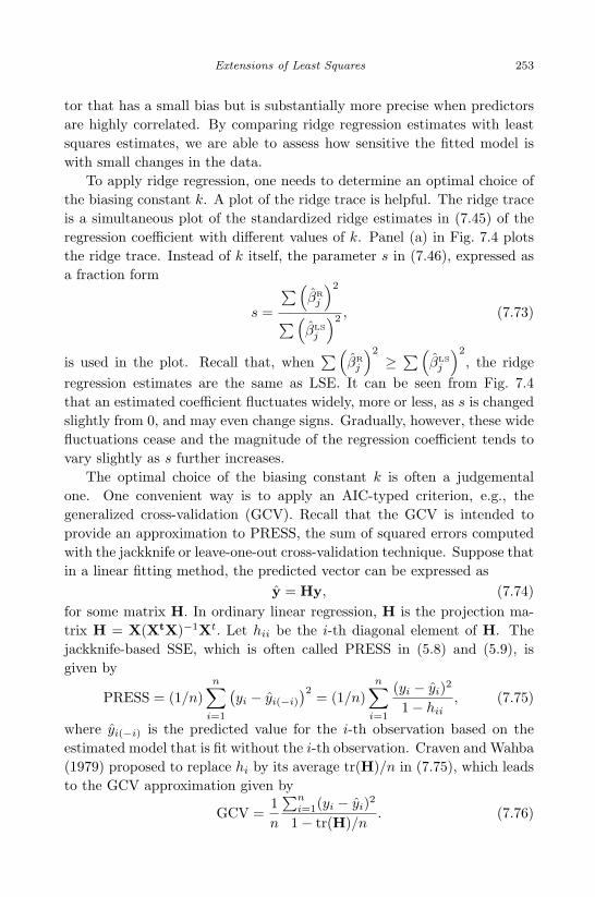
April 29, 2009 11:50 World Scientific Book - 9in x 6in Regression˙master
Extensions of Least Squares 253
tor that has a small bias but is substantially more precise when predictorsare highly correlated. By comparing ridge regression estimates with leastsquares estimates, we are able to assess how sensitive the fitted model iswith small changes in the data.
To apply ridge regression, one needs to determine an optimal choice ofthe biasing constant k. A plot of the ridge trace is helpful. The ridge traceis a simultaneous plot of the standardized ridge estimates in (7.45) of theregression coefficient with different values of k. Panel (a) in Fig. 7.4 plotsthe ridge trace. Instead of k itself, the parameter s in (7.46), expressed asa fraction form
s =
∑(βR
j
)2
∑ (βLS
j
)2 , (7.73)
is used in the plot. Recall that, when∑(
βRj
)2
≥ ∑(βLS
j
)2
, the ridgeregression estimates are the same as LSE. It can be seen from Fig. 7.4that an estimated coefficient fluctuates widely, more or less, as s is changedslightly from 0, and may even change signs. Gradually, however, these widefluctuations cease and the magnitude of the regression coefficient tends tovary slightly as s further increases.
The optimal choice of the biasing constant k is often a judgementalone. One convenient way is to apply an AIC-typed criterion, e.g., thegeneralized cross-validation (GCV). Recall that the GCV is intended toprovide an approximation to PRESS, the sum of squared errors computedwith the jackknife or leave-one-out cross-validation technique. Suppose thatin a linear fitting method, the predicted vector can be expressed as
y = Hy, (7.74)for some matrix H. In ordinary linear regression, H is the projection ma-trix H = X(XtX)−1Xt. Let hii be the i-th diagonal element of H. Thejackknife-based SSE, which is often called PRESS in (5.8) and (5.9), isgiven by
PRESS = (1/n)n∑
i=1
(yi − yi(−i)
)2 = (1/n)n∑
i=1
(yi − yi)2
1− hii, (7.75)
where yi(−i) is the predicted value for the i-th observation based on theestimated model that is fit without the i-th observation. Craven and Wahba(1979) proposed to replace hi by its average tr(H)/n in (7.75), which leadsto the GCV approximation given by
GCV =1n
∑ni=1(yi − yi)2
1− tr(H)/n. (7.76)

April 29, 2009 11:50 World Scientific Book - 9in x 6in Regression˙master
254 Linear Regression Analysis: Theory and Computing
0.00 0.02 0.04 0.06 0.08 0.10
−1.
00.
00.
51.
01.
52.
02.
5(a)
k
coef
ficie
nts
GNP.deflatorGNPUnemployedArmed.ForcesPopulationYear
min.GCV at k=0.005
0.00 0.02 0.04 0.06 0.08 0.10
7e−
048e
−04
9e−
041e
−03
(b)
k
GC
V
min.GCV at k=0.005
Fig. 7.4 Ridge Regression for Longley’s (1967) Economic Data: (a) Plot of Parameter
Estimates Versus s; (b) Plot of GCV Values Versus s.
The quantity tr(H) is referred to the effective number of degrees of free-dom. GCV, which is asymptotically equivalent to AIC and Cp, has beenwidely used as a model selection criterion in modern statistical applications.Again, it is important to note that equation (7.75) holds and hence the def-inition of GCV applies in a wide variety of problems that go far beyondordinary linear regression. Similar results are also available for the leaving-

May 7, 2009 10:22 World Scientific Book - 9in x 6in Regression˙master
Extensions of Least Squares 255
Table 7.6 Ridge Regression and LASSO for Longley’s (1967)Data.
(a) The Ridge Regression Results When k = 0.005.
Standard t Test Two-SidedEstimate Error Statistic P-Value
GNP.deflator −0.0031 0.0414 −0.0758 0.9396GNP −0.4768 0.3171 −1.5038 0.1326Unemployed −0.4505 0.0066 −68.0210 0.0000Armed.Forces −0.1836 0.0013 −145.6954 0.0000Population −0.2323 0.0968 −2.4009 0.0164Year 2.0263 0.1732 11.6987 0.0000
(b) The Ridge Regression Results When k = 0.03.
Standard t Test Two-SidedEstimate Error Statistic P-Value
GNP.deflator 0.0627 0.0285 2.1996 0.0278GNP 0.2191 0.0298 7.3520 0.0000Unemployed −0.3387 0.0022 −156.7838 0.0000Armed.Forces −0.1487 0.0014 −102.8985 0.0000Population −0.1954 0.0369 −5.2883 0.0000Year 1.1408 0.0499 22.8567 0.0000
(c) LASSO Fit with s = 1.904 or Fraction of 43.43%.The Lagrangian for the Bound Is 0.02541.
Standard t Test Two-SidedEstimate Error Statistic P-Value
GNP.deflator 0.000 0.298 0.000 1.000GNP 0.000 0.992 0.000 1.000Unemployed −0.378 0.132 −2.871 0.004Armed.Forces −0.146 0.041 −3.526 0.000Population −0.048 0.512 −0.095 0.925Year 1.331 0.502 2.650 0.008
several-out cases or the general v-fold cross-validation. In ridge regression,for a given k, we have
df = tr(H) = trX(XtX + kI)−1Xt
=p∑
j=1
d2j
d2j + k
, (7.77)
in view of (7.62).Figure 7.4(b) plots the GCV values for different choices of s in Longley’s

April 29, 2009 11:50 World Scientific Book - 9in x 6in Regression˙master
256 Linear Regression Analysis: Theory and Computing
data example. The minimum GCV occurs at s = 0.005. Panel (a) of Table7.6 gives the ridge estimates at s = 0.005. In contrast to the least squaresestimates, there are two remarkable issues. First, the slope estimate forGNP.deflator has changed sign while remaining insignificant. Secondly,Population now becomes significant. Nevertheless, from the ridge traceplot in Fig. 7.4(a), the performance of ridge estimates is not stable yet ats = 0.005.
There are two other alternative ways of determining k in the literature.The HKB (Hoerl, Kennard, and Baldwin, 1975) estimator of k is given as
k =n · σ2
‖ βLS ‖2
,
where σ2 is the unbiased estimate of the error variance from ordinary leastsquares (OLS). The rationale behind this choice of k is to provide a smallerMSE than that of OLS, which occurs when k < σ2/ ‖ β ‖2 . Farebrother(1975) observed that if XtX = I, then MSE is minimized at this value ofk. In various other examples, k generated approximately the minimal valueof MSE even when XtX 6= I. Hoerl, Kennard, and Baldwin (1975) showsthat significant improvement over OLS in terms of MSE is obtained with k.Lawless and Wang (1976) also proposed a method, the L-M estimator of k,based on the connection between ridge regression and principal componentsanalysis. All these three selection methods for k are available in the Rfunction lm.ridge.
The HKB estimate of s in this example is 0.0038, which is close to thechoice supplied by minimum GCV. The L-M estimate of s is 0.03. After all,the ridge trace in Fig. 7.4(a) provides an ultimate demonstration of howsensitive the coefficient estimates are with different choices of s. Quite afew interesting observations can be taken from the plot of the ridge trace.The slope for Armed.Forces, which is the least collinear variable, remainsunaltered with varying s. Year has a constantly positive strong effect whileUnemployed has a negative effect. The wrong negative sign of GNP haschanged to positive as s increases. Accordingly, Hoerl and Kennard (1970)suggest to pick up a k value from the ridge trace plot by inspecting whenthe system stabilizes and has the general characteristics of an orthogonalsystem. They deem this to be the best method for selecting an admissiblevalue of s. In this example, s = 0.03, also suggested by L-M, seems anappropriate and favorable choice. Panel (b) of Table 7.6 gives the ridgeestimates at s = 0.03, the choice of the L-M method. Interestingly, allpredictors become significant in the model. All slopes except the one for
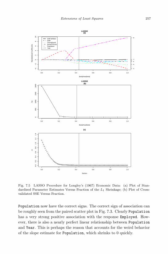
April 29, 2009 11:50 World Scientific Book - 9in x 6in Regression˙master
Extensions of Least Squares 257
* * * * * * * * * * *
0.0 0.2 0.4 0.6 0.8 1.0
−4
−2
02
46
810
(a)
|beta|/max|beta|
Sta
ndar
dize
d C
oeffi
cien
ts
*
* * *
* * * *
*
*
*
* * * ** * * * * * *
* * * * * * * * * * ** * * * * *
* * * * ** * * *
* *
* *
*
**
LASSO
23
41
6
GNP.deflatorGNPUnemployedArmed.ForcesPopulationYear
0.0 0.2 0.4 0.6 0.8 1.0
050
010
0015
0020
00
LASSO
|beta|/max|beta|
Cp
(b)
0.0 0.2 0.4 0.6 0.8 1.0
0.0
0.2
0.4
0.6
0.8
1.0
1.2
1.4
fraction
cv
(c)
Fig. 7.5 LASSO Procedure for Longley’s (1967) Economic Data: (a) Plot of Stan-dardized Parameter Estimates Versus Fraction of the L1 Shrinkage; (b) Plot of Cross-validated SSE Versus Fraction.
Population now have the correct signs. The correct sign of association canbe roughly seen from the paired scatter plot in Fig. 7.3. Clearly Population
has a very strong positive association with the response Employed. How-ever, there is also a nearly perfect linear relationship between Population
and Year. This is perhaps the reason that accounts for the weird behaviorof the slope estimate for Population, which shrinks to 0 quickly.
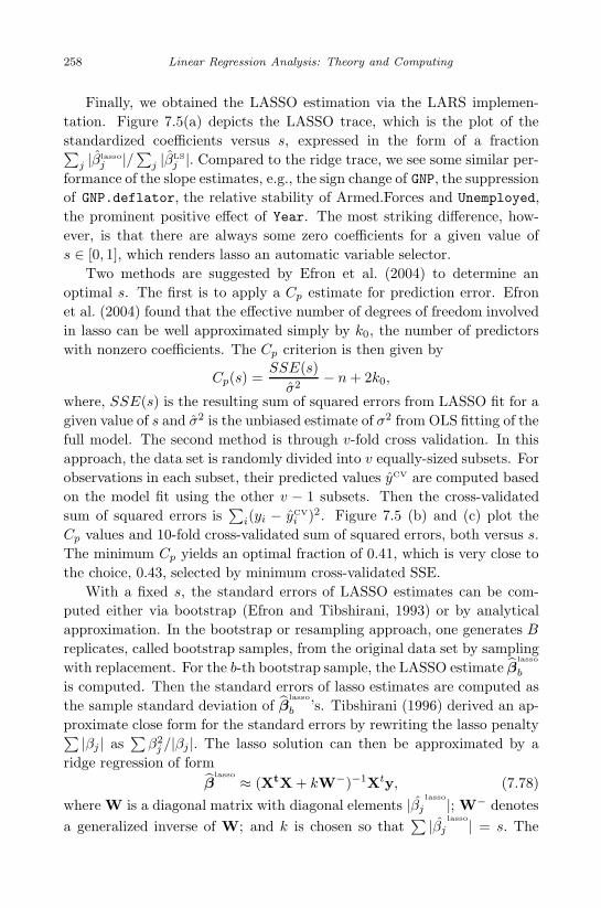
May 7, 2009 10:22 World Scientific Book - 9in x 6in Regression˙master
258 Linear Regression Analysis: Theory and Computing
Finally, we obtained the LASSO estimation via the LARS implemen-tation. Figure 7.5(a) depicts the LASSO trace, which is the plot of thestandardized coefficients versus s, expressed in the form of a fraction∑
j |βlassoj |/∑j |βLS
j |. Compared to the ridge trace, we see some similar per-formance of the slope estimates, e.g., the sign change of GNP, the suppressionof GNP.deflator, the relative stability of Armed.Forces and Unemployed,the prominent positive effect of Year. The most striking difference, how-ever, is that there are always some zero coefficients for a given value ofs ∈ [0, 1], which renders lasso an automatic variable selector.
Two methods are suggested by Efron et al. (2004) to determine anoptimal s. The first is to apply a Cp estimate for prediction error. Efronet al. (2004) found that the effective number of degrees of freedom involvedin lasso can be well approximated simply by k0, the number of predictorswith nonzero coefficients. The Cp criterion is then given by
Cp(s) =SSE(s)
σ2− n + 2k0,
where, SSE(s) is the resulting sum of squared errors from LASSO fit for agiven value of s and σ2 is the unbiased estimate of σ2 from OLS fitting of thefull model. The second method is through v-fold cross validation. In thisapproach, the data set is randomly divided into v equally-sized subsets. Forobservations in each subset, their predicted values yCV are computed basedon the model fit using the other v − 1 subsets. Then the cross-validatedsum of squared errors is
∑i(yi − yCV
i )2. Figure 7.5 (b) and (c) plot theCp values and 10-fold cross-validated sum of squared errors, both versus s.The minimum Cp yields an optimal fraction of 0.41, which is very close tothe choice, 0.43, selected by minimum cross-validated SSE.
With a fixed s, the standard errors of LASSO estimates can be com-puted either via bootstrap (Efron and Tibshirani, 1993) or by analyticalapproximation. In the bootstrap or resampling approach, one generates B
replicates, called bootstrap samples, from the original data set by samplingwith replacement. For the b-th bootstrap sample, the LASSO estimate β
lasso
b
is computed. Then the standard errors of lasso estimates are computed asthe sample standard deviation of β
lasso
b ’s. Tibshirani (1996) derived an ap-proximate close form for the standard errors by rewriting the lasso penalty∑ |βj | as
∑β2
j /|βj |. The lasso solution can then be approximated by aridge regression of form
βlasso ≈ (XtX + kW−)−1Xty, (7.78)
where W is a diagonal matrix with diagonal elements |βjlasso|; W− denotes
a generalized inverse of W; and k is chosen so that∑ |βj
lasso| = s. The

April 29, 2009 11:50 World Scientific Book - 9in x 6in Regression˙master
Extensions of Least Squares 259
covariance matrix of the lasso estimates can then be approximated by
σ2lasso · (XtX + kW−)−1XtX(XtX + kW−)−1, (7.79)
where σ2lasso is an estimate of the error variance. Clearly, this approximation
suggests an iterative way to compute the lasso estimates by alternating theestimates of W and β
lasso. Besides, equation (7.78) implies a linear form
of the predicted vector; hence GCV in (7.76) can be applied. A difficultywith the formula (7.79), however, is that the standard errors for zero co-efficient estimates are all zeroes. To get around this difficulty, Osborne,Presnell, and Turlach (2000b) proposed a smooth approximation methodfor estimating the lasso standard errors.
Panel (c) in Table 7.5 presents the LASSO fit at s = 1.904 with a frac-tion 43% out of the saturated |βLS|, a choice suggested by minimum cross-validated SSE. The standard errors are estimated via bootstrap. The modelfit roughly corresponds to keeping just four of the predictors: Unemployed,Armer.Forces, Population, and Year, although Population appears tobe rather insignificant. This selection is somewhat different from the bestsubset selection in Table 7.4 (c). The variable GNP is included in the bestsubset, significant with a wrong sign, but does not show up in the lasso fit.Notice that the coefficients in the lasso fit have been shrunk in absolutevalue, which results in reduced significance.
7.4 Parametric Nonlinear Regression
Given data (yi,xi) : i = 1, . . . , n, where yi is a continuous response andxi is the predictor vector containing mixed types of variables, one mayconsider model
yi = h(β,xi) + εi with εii.i.d.∼ N (0, σ2), (7.80)
where the function h(·) is assumed to have a fully specified nonlinear formup to the parameter vector β ∈ Rp. This model is generally termed as aparametric nonlinear model. If, on the other hand, the form of h(·) is leftcompletely or partially unspecified, it would result in a nonparametric orsemiparametric nonlinear model, which are often approached with kernel-or spline-based smoothing techniques. The additive model (AM) discussedin Section 6.2 is of the semiparametric type. In this section, we focus onparametric nonlinear models only. Detailed treatment of nonparametricnonlinear models is beyond the scope of this text.

April 29, 2009 11:50 World Scientific Book - 9in x 6in Regression˙master
260 Linear Regression Analysis: Theory and Computing
(a)
C
B=0.5B=1B=5
(b)
C
A=0.5A=1A=5
Fig. 7.6 Plot of the Logistic Function With C = 1: (a) When B Varies With A = 1;(b) When A Varies With B = 1.
Linear regression may fit poorly to data that show a strong nonlin-ear pattern, which calls for the need of fitting nonlinear models. Thereare a broad range of nonlinear functions available. The specific functionalforms employed in a study are often derived on the basis of both scientificconsiderations and empirical evidences. The parameters involved usuallyhave direct and meaningful interpretation in terms of the application back-ground. For example, the general logistic function has three parameters(A, B,C):
f(x) =C
1 + A · exp(−Bx)=
C · exp(Bx)exp(Bx) + A
, (7.81)
where C is the limiting value of the curve; the parameter B controls themonotonicity of the curve, a positive B corresponding to an increasing

May 7, 2009 10:22 World Scientific Book - 9in x 6in Regression˙master
Extensions of Least Squares 261
function and a negative B for a decreasing relationship; the parameter A
controls the rate of change. Figure 7.6 plots the logistic function for someselected parameter values. The logistic function has a sigmoid shape. Thistype of functions are often seen in describing certain kinds of growth, whichthe growth rate of growth becomes progressively smaller over time.
Another advantage of using a parametric nonlinear model is that it hasthe convenience to enforce some desired constraints that are, otherwise,hard to do for linear regression. For example, the mean response may bedesired to be positive or stay within certain range, which can be easilybuilt in a nonlinear model. Many nonlinear functions can also achieve anasymptote or limiting value as X approaches a certain value.
7.4.1 Least Squares Estimation in Nonlinear Regression
The least squares (LS) method can be used to fit nonlinear models, inwhich case it is termed as nonlinear least squares . The nonlinear LSE β isobtained by minimizing the same objective function
Q(β) =n∑
i=1
yi − h(β,xi)2
as in linear regression. However, fitting a nonlinear model is more involved.Due to the nonlinearity of h(·), there is no general close-form solution ofβ. The optimization of Q(β) is typically done with numerical iterativealgorithms.
Assume that Q has continuous first and second derivatives in the sensethat its gradient vector of Q
g = Q′(β) =∂Q
∂β= −2
n∑i=1
yi − h(β,xi) ∂h
∂β
and its Hessian matrix
H = Q′′(β) =∂2Q
∂β∂β′ =(
∂2Q
∂βj∂βj′
)(7.82)
both have continuous components. The nonlinear LSE β is basically astationary point of Q, satisfying g(β) = 0. In order for β to be a localminimizer of Q, we further assume that the Hessian matrix H is positivedefinite at β.
A numerical algorithm updates an initial guess β(0) iteratively with thegeneral form
β(k+1) = β(k) + a(k)d(k),

April 29, 2009 11:50 World Scientific Book - 9in x 6in Regression˙master
262 Linear Regression Analysis: Theory and Computing
where d(k) satisfying ‖ d ‖= 1 is the step direction and the scalar a(k) iscalled the step size or step length. If there exists a δ such that Q(β(k+1)) =β(k) + a(k)d(k) < Q(β(k)) for any a ∈ (0, δ), we say that the step d(k) isacceptable. The following theorem (Bard, 1974) characterizes acceptabledirections by establishing a necessary and sufficient condition.
Theorem 7.5. A direction d(k) is acceptable if and only if there exists apositive definite matrix R such that
d(k) = −Rg(β(k)).
Various optimization methods usually differ in their criteria used to findthe step directions and step sizes. In particular, methods that have stepdirections of the form given in Theorem 7.5 are called the gradient methods.
The Newton-Raphson method is the most commonly used gradient al-gorithm for optimization. To motivate, consider the Taylor’s expansion ofg(β) at an initial guess β:
0 = g(β) = g(β) + H(β)(β − β
).
Solving it for β leads to the updating formula:
β(k+1) = β(k) −H(β(k))
−1
g(β(k)). (7.83)
However, it can be difficult to supply explicit derivative formula for acomplicated function h(·). One solution, known as a DUD (Does not UseDerivatives) algorithm, approximates the derivatives by a finite-differencemethod. Take a one-dimensional function g(x) for instance. The finitedifference method numerically approximate its first derivative
g′(x) = limt→0
g(x + t)− g(x)t
by
g′(x) ≈ g(x + t)− g(x)t
for a small value of t. Nevertheless, the approximation from the DUDalgorithm is known to perform poorly when the model function h(·) is notwell behaved.
Under some mild regularity conditions as given in Amemiya (1985), thenonlinear LSE β is asymptotically normally distributed as
β ∼ N
β, Cov(β)
, (7.84)

May 7, 2009 10:22 World Scientific Book - 9in x 6in Regression˙master
Extensions of Least Squares 263
where Cov(β) denotes the asymptotic variance-covariance matrix of β. De-note
F = (Fij)n×p =(
∂h(β,xi)∂βj
).
It can be shown to be
Cov(β) = σ2(FtF
)−1 (7.85)
The error variance σ2 can be estimated in the similar manner as
σ2 =SSE
n− p=
∑ni=1
yi − h(β,xi)
2
n− p.
Substituting (β, σ2) for (β, σ2) in (7.85) yields estimates for the variance-covariance matrix for β. Statistical inference on β, as well as atβ, canbe made accordingly. At a given x, confidence intervals for predictionpurposes, i.e., estimating h(β,x), are also available via the delta method ,as we shall illustrate in the following example.
7.4.2 Example
To illustrate, we consider an example taken from (Fox, 2002), pertainingto the US population growth. The data set contains the decennial censuspopulation data in the United States of America from 1970 through 1990.It is interesting to study the growth pattern of population (in millions)over years. Figure 7.7 (a) plots the population size (Y ) versus year (X),exhibiting a strong curvature. The superimposed LS straight line y =−35.65409 + 12.13828x clearly does not seem to provide a satisfactory fit,as also evidenced by the systematic pattern shown in the residual plot givenby Fig. 7.7(b).
We consider a logistic function of special form
yi =β1
1 + exp(β2 + β3xi)+ εi,
where yi is the population size at time xi; β1 is the asymptote towardswhich the population grows; β2 reflects the size of the population at timex = 0 relative to its asymptote; and β3 controls the growth rate of thepopulation.
Nonlinear regression can be fit with PROC NLIN in SAS or the R func-tion nls() in the nls library. In this illustrate, we shall only discuss PROC

April 29, 2009 11:50 World Scientific Book - 9in x 6in Regression˙master
264 Linear Regression Analysis: Theory and Computing
1800 1850 1900 1950
050
100
150
200
250
(a)
year
popu
latio
n
1800 1850 1900 1950−2
0−1
00
1020
3040
(b)
year
resi
dual
s(lm
.fit)
1800 1850 1900 1950
050
100
150
200
250
(c)
popu
latio
n
1800 1850 1900 1950
−50
5
(d)
resi
dual
s(po
p.m
od)
Fig. 7.7 Parametric Nonlinear Regression with the US Population Growth Data Re-produced from Fox (2002): (a) Scatter Plot of the Data Superimposed by the LS FittedStraight Line; (b) Plot of the Residuals From the Linear Model Versus Year; (c) ScatterPlot of the Data Superimposed by the Fitted Nonlinear Curve; (d) Plot of the ResidualsFrom the Nonlinear Fit Versus Year.
NLIN in SAS. One is referred to Fox (1997) and Fox (2002) for an R exam-ple. The PROC NLIN procedure has the METHOD= option for the user tosupply derivatives or let SAS calculate them. By default, the derivatives arecomputed with numerical differentiation. The common suggestion in SASis to avoid DUD if possible and, instead, choose METHOD=NEWTON,or METHOD=MARQUARDT when the parameter estimates are highlycorrelated. The latter option METHOD=MARQUARDT applies theLevenberg-Marquardt method to handle the singularity problem of the Hes-

April 29, 2009 11:50 World Scientific Book - 9in x 6in Regression˙master
Extensions of Least Squares 265
sian matrix H(β(k)) during iteration.Another important issue in numerical optimization is the starting points
for the parameters. PROC NLIN allows the user to specify a grid of startingvalues. SAS calculates the initial sum of squared errors for each combina-tion and then starts the iterations with the best set.
Table 7.7 Nonlinear Regression Results of the US Pop-ulation Data from PROC NLIN and PROC AUTOREG.
(a) Parameter Estimates from the NLIN Procedure
Approx Approximate 95%Parameter Estimate Std Error Confidence Limits
β1 389.2 30.8121 324.4 453.9β2 3.9903 0.0703 3.8426 4.1381β3 −0.2266 0.0109 −0.2494 −0.2038
(b) Approximate Correlation Matrix
β1 β2 β3
β1 1.0000000 −0.1662384 0.9145423
β2 −0.1662384 1.0000000 −0.5406492
β3 0.9145423 −0.5406492 1.0000000
(c) Durbin-Watson Statistics for First-order AutocorrelationAmong Residuals: PROC AUTOREG.
Order DW Pr < DW Pr > DW
1 0.6254 < .0001 1.0000
Table 7.7 presents the fitted results. The fitted logistic growth modelfor US population size is found to be
h(x) =389.2
1 + exp(3.99− 0.23 · x),
which has been added to the scatter plot in Fig. 7.4(c). It gives a muchimproved fit to the data. The above equation can be used for predictionpurpose. In particular, the confidence intervals for prediction can be ob-tained via the so-called delta method :
h(β, x)± z1−α/2 ·√g(β, x)t Cov(β)g(β, x),
in view of the Taylor expansionh(β, x) = h(β, x) + g(β, x)t (β − β) + o
(‖ β − β ‖
).
May 7, 2009 10:22 World Scientific Book - 9in x 6in Regression˙master
266 Linear Regression Analysis: Theory and Computing
The estimated correlation matrix is presented in Penal (b) of Table 7.7.Multiplying it by σ2 = MSE = 19.8025 would give the estimated covari-ance matrix.
Figure 7.7 (d) gives the residual plot from the nonlinear model fit. It canbe seen that the systematic pattern due to lack-of-fit in the mean functionhas mostly been eliminated. Nevertheless, the residual seems to fluctuatecyclically with time. The Durbin-Watson statistic is used to test for auto-correlation and lack of independence of residuals, which are commonly seenin time series data. The test statistic provided by PROC AUTOREG inSAS ranges from 0 to 4. A value close to 2.0 indicates no strong evidenceagainst the null hypothesis of no autocorrelation. The first-order Durbin-Watson statistic is printed by default. This statistic can be used to testfor first-order autocorrelation. The DWPROB option prints the p-valuesfor the Durbin-Watson test. Since these p-values are computationally ex-pensive, they are not reported by default. One can also use the DW=option to request higher-order Durbin-Watson statistics, called generalizedDurbin-Watson statistics, for testing higher-order autocorrelations.
Panel (c) Table 7.7 presents the results from PROC AUTOREG. Notethat Pr < DW is the p-value for testing positive autocorrelation, andPr > DW is the p-value for testing negative autocorrelation. Thus theresiduals from the nonlinear fit shows a statistically significant (with p-value < .0001) first-order positive autocorrelation.
Problems
1. Consider the non-full-rank model y = Xβ + ε, where X is n× (k + 1)of rank p and ε ∼ (0, σ2I). Show that a linear function of β, λtβ, isestimable if and only if any of the following equivalent conditions ismet:
(a) λ ∈ C(XtX), the column space of XtX; or, equivalently, λt ∈R(XtX), the row space of XtX.
(b) λ such that
XtX(XtX)−λ = λ or λt(XtX)−XtX = λt
2. Using Guass-Markov Thoerem, prove Corollary 7.2.3. Consider estimable functions Λβ, where Λ be an m × (k + 1) matrix
with rows λti for i = 1, . . . , m.
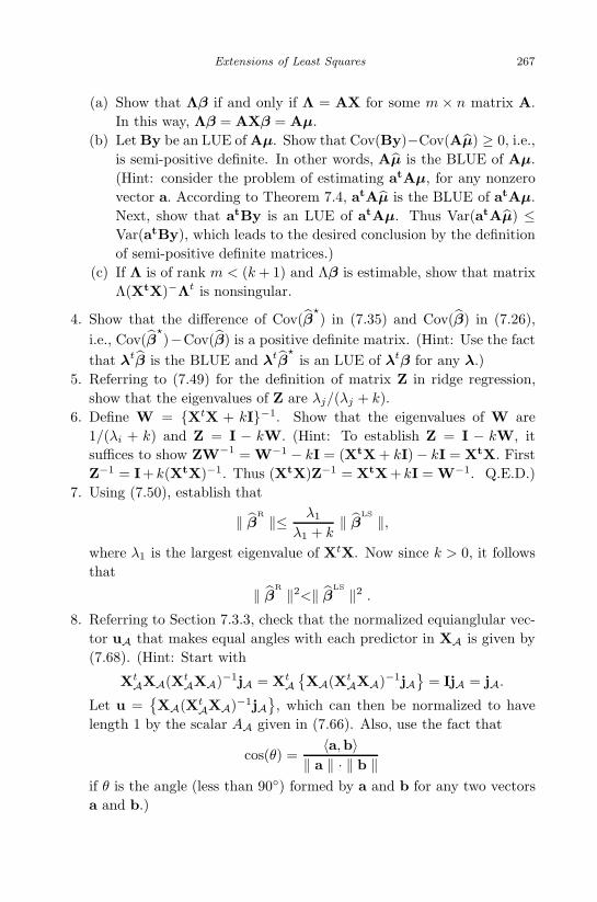
May 7, 2009 10:22 World Scientific Book - 9in x 6in Regression˙master
Extensions of Least Squares 267
(a) Show that Λβ if and only if Λ = AX for some m × n matrix A.
In this way, Λβ = AXβ = Aµ.
(b) Let By be an LUE of Aµ. Show that Cov(By)−Cov(Aµ) ≥ 0, i.e.,is semi-positive definite. In other words, Aµ is the BLUE of Aµ.
(Hint: consider the problem of estimating atAµ, for any nonzerovector a. According to Theorem 7.4, atAµ is the BLUE of atAµ.Next, show that atBy is an LUE of atAµ. Thus Var(atAµ) ≤Var(atBy), which leads to the desired conclusion by the definitionof semi-positive definite matrices.)
(c) If Λ is of rank m < (k + 1) and Λβ is estimable, show that matrixΛ(XtX)−Λt is nonsingular.
4. Show that the difference of Cov(β) in (7.35) and Cov(β) in (7.26),
i.e., Cov(β)−Cov(β) is a positive definite matrix. (Hint: Use the fact
that λtβ is the BLUE and λtβ
is an LUE of λtβ for any λ.)5. Referring to (7.49) for the definition of matrix Z in ridge regression,
show that the eigenvalues of Z are λj/(λj + k).6. Define W = XtX + kI−1. Show that the eigenvalues of W are
1/(λi + k) and Z = I − kW. (Hint: To establish Z = I − kW, itsuffices to show ZW−1 = W−1 − kI = (XtX + kI)− kI = XtX. FirstZ−1 = I+ k(XtX)−1. Thus (XtX)Z−1 = XtX+ kI = W−1. Q.E.D.)
7. Using (7.50), establish that
‖ βR ‖≤ λ1
λ1 + k‖ β
LS ‖,where λ1 is the largest eigenvalue of XtX. Now since k > 0, it followsthat
‖ βR ‖2<‖ β
LS ‖2 .
8. Referring to Section 7.3.3, check that the normalized equianglular vec-tor uA that makes equal angles with each predictor in XA is given by(7.68). (Hint: Start with
XtAXA(Xt
AXA)−1jA = XtAXA(Xt
AXA)−1jA
= IjA = jA.
Let u =XA(Xt
AXA)−1jA, which can then be normalized to have
length 1 by the scalar AA given in (7.66). Also, use the fact that
cos(θ) =〈a,b〉
‖ a ‖ · ‖ b ‖if θ is the angle (less than 90) formed by a and b for any two vectorsa and b.)

April 29, 2009 11:50 World Scientific Book - 9in x 6in Regression˙master
This page intentionally left blankThis page intentionally left blank

April 29, 2009 11:50 World Scientific Book - 9in x 6in Regression˙master
Chapter 8
Generalized Linear Models
Linear regression has wide and fundamental applications in various fields.Its popularity can be attributed to its simple form, sound theoretical sup-port, efficient computation in estimation, great flexibility to incorporateinteractions, dummy variables, and other transformations, and easy inter-pretations. For all the linear models discussed so far, the response Y isa continuous variable. Many studies or experiments are often involve re-sponses of other types. Consider, for example, evaluation of the academicperformance of college students. Instead of the continuous grade pointaverage (GPA) score, the categorical grade A–F may have been used. Gen-eralized linear models (GLM; McCullagh and Nelder, 1983) extends linearregression to encompass other types of response while, at the same time,enjoying nearly all the merits of linear modeling.
In this chapter, we study how linear regression is generalized to handledata with different types of responses. We first motivate the problem usingan example on simple logistic regression in Section 8.1, followed by generaldiscussion on the basic components (Section 8.2), estimation (Section 8.3),statistical inference, and other issues (Section 8.4) in GLM. We then in-troduce two important and very commonly used GLMs, logistic regressionmodels for binary responses in Section 8.5 and log-linear models for countdata in Section 8.6.
8.1 Introduction: A Motivating Example
We first reproduce an example from Hosmer and Lemeshow (2000) thatgives an excellent motivation to the problem with a real application. Thedata set, which can be downloaded at
ftp://ftp.wiley.com/public/sci−tech−med/logistic/alr.zip,
269

April 29, 2009 11:50 World Scientific Book - 9in x 6in Regression˙master
270 Linear Regression Analysis: Theory and Computing
20 30 40 50 60 70
0.0
0.2
0.4
0.6
0.8
1.0
(a)
age
CH
D
30 40 50 60
0.1
0.2
0.3
0.4
0.5
0.6
0.7
0.8
(b)
age
prop
ortio
n C
HD
Fig. 8.1 (a) Scatterplot of the CHD Data, Superimposed With the Straight Line fromLeast Squares Fit; (b) Plot of the Percentage of Subjects With CHD Within Each AgeGroup, Superimposed by LOWESS Smoothed Curve.
was collected from a retrospective coronary heart disease (CHD) study.It contains three variables: ID for each subject, AGE (X), and a binaryindicator CHD (Y ) indicating whether CHD occurs to the subject. Theobjective is to explore the relationship between age and prevalence of CHD.
A scatterplot of the data is given in Fig. 8.1(a). Although one can seelarger values of AGE tend to be more associated with “1”’s of CHD, the

May 7, 2009 10:22 World Scientific Book - 9in x 6in Regression˙master
Generalized Linear Models 271
plot is not very informative due to discreteness of the response Y .Recall that linear regression relates the conditional mean of the re-
sponse, E(Y |X), to a linear combination of predictors. Can we do thesame with binary data? Let the binary response yi = 1 if CHD is found inthe ith individual and 0 otherwise for i = 1, . . . , n. Denote πi = Pr(yi = 1).Thus, the conditional distribution of yi given xi is a Bernoulli trial withparameter πi. It can be found that E(yi) = πi. Hence, the linear modelwould be
E(yi) = πi = β0 + β1xi. (8.1)
Figure 8.1(a) plots the straight line fitted by least squares. Clearly, it isnot a good fit. There is another inherent problem with Model (8.1). Theleft-hand side πi ranges from 0 to 1, which does not mathematically matchwell with the range (−∞,∞) of the linear equation on the right-hand side.A transformation on πi, g(·), which maps [0, 1] onto (−∞,∞), would help.This transformation function is referred to the link function.
In order to explore the functional form between πi and xi, we musthave available estimates of the proportions πi. One approach is group thedata by categorizing AGE into several intervals and record the relativelyfrequency of CHD within each interval. Table 8.1 shows the worksheet forthis calculation.
Table 8.1 Frequency Table of AGE Group by CHD.
CHDAge Group n Absent Present Proportion
20-29 10 9 1 0.1030-34 15 23 2 0.1335-39 12 9 3 0.2540-44 15 10 5 0.3345-49 13 7 6 0.4650-54 8 3 5 0.6355-59 17 4 13 0.7660-69 10 2 8 0.80
Total 100 57 43 0.43
Figure 8.1(b) plots the proportions of subjects with CHD in each ageinterval versus the middle value of the interval. It can be seen that theconditional mean of yi or proportion gradually approaches zero and one toeach end. The plot shows an ‘S’-shaped or sigmoid nonlinear relationship,in which the change in π(x) with per unit increase in x grows quickly at first,but gradually slows down and then eventually levels off. Such a pattern is
April 29, 2009 11:50 World Scientific Book - 9in x 6in Regression˙master
272 Linear Regression Analysis: Theory and Computing
rather representative and can be generally seen in many other applications.It is often expected to see that a fixed change in x has less impact whenπ(x) is near 0 or 1 than when π(x) is near 0.5. Suppose, for example, thatπ(x) denotes the probability to pass away for a person of age x. An increaseof five years in age would have less effect on π(x) when x = 70, in whichcase π(x) is perhaps close to 1, than when x = 40.
In sum, a suitable link function g(πi) is desired to satisfy two conditions:it maps [0, 1] onto the whole real line and has the sigmoid shape. A naturalchoice for g(·) would be a cumulative distribution function of a randomvariable. In particular, the logistic distribution, whose CDF is the simplifiedlogistic function g(x) = exp(x)/1 + exp(x) in (7.81), yields the mostpopular link. Under the logistic link, the relationship between the CHDprevalence rate and AGE can be formulated by the following simple model
logit(πi) = log(
πi
1− πi
)= β0 + β1xi.
When several predictors X1, . . . , Xp are involved, the multiple logisticregression can be generally expressed as
log(
πi
1− πi
)= x′iβ.
We shall explore more on logistic regression in Section 8.5.
8.2 Components of GLM
The logistic regression model is one of the generalized linear models (GLM).Many models in the class had been well studied by the time when Nelderand Wedderburn (1972) introduced the unified GLM family. The specifica-tion of a GLM generally consists of three components: a random componentspecifies the probability distribution of the response; a systematic compo-nent forms the linear combination of predictors; and a link function relatesthe mean response to the systematic component.
8.2.1 Exponential Family
The random component assumes a probability distribution for the responseyi. This distribution is taken from the natural exponential distributionfamily of form
f(yi; θi, φ) = exp
yiθi − b(θi)a(φ)
+ c(yi; φ)
, (8.2)

April 29, 2009 11:50 World Scientific Book - 9in x 6in Regression˙master
Generalized Linear Models 273
where θi is the natural parameter and φ is termed as the dispersion param-eter. It can be shown (see Exercise 8.6.2) that
E(yi) = µi = b′(θi) and Var(yi) = b′′(θi)a(φ), (8.3)
both moments determined by the function b(·).Take the Gaussian distribution for example. The probability density
function (pdf) of N(µ, σ2) can be rewritten as
fY (y) =1√
2πσ2exp
− (y − µ)2
2σ2
= exp
yµ− µ2/2σ2
− y2/σ2 + log(2πσ2)2
.
Therefore, θ = µ, φ = σ2, a(φ) = φ, b(θ) = θ2/2, and c(y, φ) =−
y2/φ + log(2πφ)
/2.
8.2.2 Linear Predictor and Link Functions
The systematic component is the linear predictor, denoted as
ηi =∑
j
βjxij = xiβ,
for i = 1, . . . , n and j = 0, 1, . . . , p with xi0 = 1 to account for the in-tercept. Similar to ordinary linear regression, this specification allows forincorporation of interaction, polynomial terms, and dummy variables.
The link function in GLM relates the linear predictor ηi to the meanresponse µi. Thus
g(µi) = ηi
or inversely
µi = g−1(ηi).
In classical Gaussian linear models, the identity link g(µi) = µi is applied.A preferable link function usually not only maps the range of µi onto thewhole real line, but also provides good empirical approximation and carriesmeaningful interpretation when it comes to real applications.
As an important special case, the link function g such that
g(µi) = θi
is called the canonical link. Under this link, the direct relationship θi = ηi
occurs. Since µi = b′(θi), we have θi = (b′)−1(µi). Namely, the canonicallink is the inverse of b′(·):
(b′)−1(µi) = ηi =∑
j
βjxij . (8.4)

April 29, 2009 11:50 World Scientific Book - 9in x 6in Regression˙master
274 Linear Regression Analysis: Theory and Computing
In Gaussian linear models, the canonical link is the identity function. Withthe canonical link, the sufficient statistic is Xty in vector notation with com-ponents
∑i xijyi for j = 0, 1, . . . , p. The canonical link provides mathemat-
ical convenience in deriving statistical properties of the model; at the sametime, they are also often found eminently sensible on scientific grounds.
8.3 Maximum Likelihood Estimation of GLM
The least squares (LS) method is no longer directly appropriate when the re-sponse variable Y is not continuous. Estimation of GLM is processed withinthe maximum likelihood (ML) framework. However, as we will see, the MLestimation in GLM has a close connection with an iteratively weighted leastsquares method.
Given data (yi,xi) : i = 1, . . . , n, the log likelihood function is
L(β) =∑
i
Li =∑
i
log fY (yi; θi, φ) =∑
i
yiθi − b(θi)a(φ)
+∑
i
c(yi, φ). (8.5)
8.3.1 Likelihood Equations
The likelihood equations are∂L(β)∂βj
=∑
i
∂Li
∂βj= 0
for j = 0, 1, . . . , p. Using the chain rule, we have∂Li
∂βj=
∂Li
∂θi
∂θi
∂µi
∂µi
∂ηi
∂ηi
∂βj,
where∂Li
∂θi=
yi − b′(θi)a(φ)
=yi − µi
a(φ)using µi = b′(θi);
∂θi
∂µi= b′′(θi) = Var(yi)/a(φ) using Var(yi) = b′′(θi)a(φ);
∂µi
∂ηi= (g−1)′(ηi);
and∂ηi
∂βj= xij .
Therefore, the likelihood equations for β becomen∑
i=1
(yi − µi)xij
Var(yi)· ∂µi
∂ηi= 0, for j = 0, 1, . . . , p. (8.6)

April 29, 2009 11:50 World Scientific Book - 9in x 6in Regression˙master
Generalized Linear Models 275
In the case of a canonical link ηi = θi, we have∂µi
∂ηi=
∂µi
∂θi=
∂b′(θi)∂θi
= b′′(θi).
Thus∂Li
∂βj=
yi − µi
Var(yi)b′′(θi)xij =
(yi − µi)xij
a(φ)(8.7)
using (8.3) and the likelihood equations simplify to∑
i
xijyi =∑
i
xijµi, for j = 0, 1, . . . , p.
Or in matrix notations, Xt(y − µ) = 0, which is in the same form as seenin ordinary linear regression
XtXβ = Xty =⇒ Xt(y −Xβ) = Xt(y − µ) = 0.
8.3.2 Fisher’s Information Matrix
Fisher’s information matrix I is defined as the negative expectation of thesecond derivatives of the log-likelihood with respect to β, i.e., I = E(−L′′)with elements E−∂2L(β)/∂βj∂βj′.
Using the general likelihood results
E
(∂2Li
∂βj∂βj′
)= −E
(∂Li
∂βj
∂Li
∂βj′
),
which holds for distributions in the exponential family (Cox and Hinkley,1974, Sec. 4.8), we have
E
(∂Li
∂βj
∂Li
∂βj′
)= −E
(yi − µi)xij
Var(yi)∂µi
∂ηi
(yi − µi)xij′
Var(yi)∂µi
∂ηi
from (8.6)
= − xijxij′
Var(yi)
(∂µi
∂ηi
)2
and hence
E
(−∂2L(β)
∂βjβj′
)=
n∑
i=1
xijxij′
Var(yi)
(∂µi
∂ηi
)2
. (8.8)
Let W = diag(wi) be the diagonal matrix with diagonal elements
wi =1
Var(yi)
(∂µi
∂ηi
)2
. (8.9)
Then the information matrix is given by
I = XtWX (8.10)
April 29, 2009 11:50 World Scientific Book - 9in x 6in Regression˙master
276 Linear Regression Analysis: Theory and Computing
If the canonical link is used, then from equation (8.7)(
∂2L(β)∂βjβj′
)= − xij
a(φ)· ∂µi
∂βj′,
which does not involve the random variable yi. This implies that(
∂2L(β)∂βjβj′
)= E
(∂2L(β)∂βjβj′
). (8.11)
In other words, the observed information matrix is equal to the expectedinformation matrix with the canonical link.
8.3.3 Optimization of the Likelihood
The log-likelihood function of a GLM is typically nonlinear in β. Optimiza-tion of the likelihood is usually done via iterative numerical algorithms suchas the Newton-Raphson method or Fisher scoring method.
Denote the maximum likelihood estimate (MLE) of β as β, which sat-isfies L′(β) = 0. Applying the first-order Taylor series expansion on L′(β)at the current estimate β(k) gives
0 = L′(β) = L′(β(k)) + L′′(β(k))(β − β(k)).
Solving the equation for β leads to the Newton-Raphson updating formulaas in (7.83)
β(k+1) = β(k) −(H(k)
)−1
u(k), (8.12)
where u(k) = L′(β(k)) is the first derivative or gradient of the log-likelihoodevaluated at β(k) and H(k) = L′′(β(k)) is its second derivative or Hessianmatrix evaluated at β(k).
Fisher scoring resembles the Newton-Raphson method, except for thatFisher scoring uses the expected value of −H(k), called the expected infor-mation, whereas Newton-Raphson applies the matrix directly, called theobserved information. Note that I(k) = E
(−H(k)). Plugging it into ex-
pression (8.12) yields the updating formula for Fisher scoring
β(k+1) = β(k) +(I(k)
)−1
u(k). (8.13)
It is worth noting that, from (8.11), the Newton-Raphson method is iden-tical to Fisher scoring under the canonical link, in which case the observedinformation is non-random and hence equal to the expected information.

May 7, 2009 10:22 World Scientific Book - 9in x 6in Regression˙master
Generalized Linear Models 277
Next, we shall show that implementation of Fisher scoring in GLM takesthe form of an iteratively reweighted least squares algorithm. The weightedleast squares (WLS; see Section 7.2) estimator of β is referred to
β = (XtV−1X)−1XtV−1z, (8.14)
when the linear model is
z = Xβ + ε
with ε ∼ (0,V).From (8.6), the component of the gradient u is
uj =n∑
i=1
(yi − µi)xij
Var(yi)·(
∂µi
∂ηi
)2
· ∂ηi
∂µi.
Hence, u can be rewritten in matrix form as
u = XtW∆(y − µ), (8.15)
where ∆ = diag (∂ηi/∂µi) and W is given in equation (8.9).Also, from equation (8.10), I = XtWX. Therefore,
β(k+1) = β(k) +(I(k))−1
u(k), where I(k) = XtW(k)X from (8.10),
= (XtW(k)X)−1XtW(k)Xβ(k) +
(XtW(k)X)−1XtW(k)∆(k)(y − µ(k))
=XtW(k)X
−1
XtW(k)Xβ(k) + ∆(k)(y − µ(k))
=XtW(k)X
−1
XtW(k)η(k) + ∆(k)(y − µ(k))
=XtW(k)X
−1
XtW(k)z(k) (8.16)
if one defines an adjusted response
z(k) = η(k) + ∆(k)(y − µ(k))
with components
z(k)i = η
(k)i +
(yi − µ
(k)i
)· ∂ηi
∂µi
∣∣∣∣β=β(k)
(8.17)
for i = 1, . . . , n. Note that z(k)i ’s are continuously scaled. Comparing (8.16)
to (8.14), it is clear that β(k+1) is the WLS solution for fitting ordinarylinear model
z(k) = Xβ(k) + ε, with ε ∼0,(W(k)
)−1
.

April 29, 2009 11:50 World Scientific Book - 9in x 6in Regression˙master
278 Linear Regression Analysis: Theory and Computing
8.4 Statistical Inference and Other Issues in GLM
8.4.1 Wald, Likelihood Ratio, and Score Test
The maximum likelihood framework is a well-established system for statis-tical inference. The maximum likelihood estimators have many attractiveproperties. For example, they are asymptotically consistent and efficient.Large-sample normality is also readily available under weak regularity con-ditions. Standard ML results supplies that
βd−→ N (
β, I−1)
or N
β,(XtWX
)−1
as n →∞ (8.18)
where the notation d−→ means “converges in distribution to.” The asymp-totic variance-covariance matrix of β is
Cov(β) = I−1 =(XtWX
)−1,
which can be estimated by replacing W with its estimate W. Anotherimmediate ML result is the so-called delta method, which can be used toobtain asymptotic distributions for any smooth function of β, g(β). Letg′ = ∂g(β)/∂β. Then
g(β) d−→ N g(β), (g′)tI−1g′
, (8.19)
where the asymptotic variance Varg(β) = g′tI−1g′ can be estimated bysubstituting β with its MLE β. This result can be heuristically justified bythe Taylor expansion
g(β)− g(β) ≈ (g′)t(β − β).
Within the ML framework, there are three commonly-used methods formaking statistical inference on β: the Wald test, the likelihood ratio test,and the score test, all exploiting the asymptotic normality of maximumlikelihood estimation. We will briefly discuss each of them from the hy-pothesis testing prospective. Confidence intervals can be generally derivedby inverting the testing procedures.
The Wald statistic for testing the null H0: Λβ = b where Λ is q×(p+1)of rank q takes a similar form seen in ordinary linear regression:
G =(Λβ − b
)tΛ
(XtWX
)−1
Λt
−1 (Λβ − b
). (8.20)
The null distribution of G is referred to χ2(q). As a special case, for H0:βj = b, the z test
z =√
G =βj − b
s.e.(βj)H0∼ N(0, 1)

April 29, 2009 11:50 World Scientific Book - 9in x 6in Regression˙master
Generalized Linear Models 279
can be used. It is most convenient to derive confidence intervals from theWald test. For example, (1− α)× 100% CI for βj is given by
βj ± z1−α2
s.e.(βj).
Clearly, Wald-typed inference is also readily available for functions of β,g(β), using results in (8.19).
The likelihood ratio test (LRT) compares the maximized log-likelihoodfunctions between two nested models. Suppose that we have a model, calledthe full model, and a null hypothesis H0. Bringing the conditions in H0 intothe full model gives a reduced model. Let Lfull and Lreduced denote theirrespective maximized log-likelihoods. The likelihood ratio test statistic is
LRT = −2 ·(Lreduced − Lfull
). (8.21)
The null distribution of LRT is again χ2(ν), where ν is the difference innumber of degrees of freedom between two models.
The third alternative for testing H0 : β = b is the score test, which isalso the Lagrange multiplier test. It is based on the slope and expectedcurvature of L(β) at the null value b. Let
u0 = u(b) =∂L
∂β
∣∣∣∣β = b
be the score function of the full model evaluated at the null value b (recallthat u(β) = 0) and
I0 = I(b) = − E
(∂2L
∂β ∂βt
)∣∣∣∣β = b
be the Fisher’s information matrix of the full model evaluated at b. Thescore test statistic is a quadratic form given as
S = ut0 I−1
0 u0. (8.22)
Under H0, the score test statistic follows the same chi-squared null dis-tribution. Consider another illustration, which is more practically use-ful. Suppose that β can be partitioned into (β1, β2)t and we want to test
H0 : β1 = b1. Let β(0)
2 denote the MLE of β2 obtained from fitting thereduced model or the null model. The score test statistic is then given by
S = ut1
(I11 − I12I−1
22 I21
)−1u1
∣∣∣β = (b1, β
(0)
2 )t, (8.23)
where
u1 =∂L
∂β1
and Ijj′ =∂2L
∂βj ∂βtj′

April 29, 2009 11:50 World Scientific Book - 9in x 6in Regression˙master
280 Linear Regression Analysis: Theory and Computing
L(β)
β
β b
Wald
score
LRT
Fig. 8.2 Plot of the Log-likelihood Function: Comparison of Wald, LRT, and ScoreTests on H0 : β = b.
for j, j′ = 1, 2. Note that all the quantities involved in the above expressionare derived from the full model but evaluated at β = (b1, β
(0)
2 )t, which areobtained from fitting the null model. The null distribution of S is χ2 withdf equal to the dimension of β1.
The Wald, LRT, and score tests all refer to the same null chi-squared dis-tribution and they can be shown to be asymptotically equivalent for largesample sizes. On the other hand, they show different empirical perfor-mances. Fig. 8.2 illustrated the comparison of these three tests for testingH0 : β = b in the one-dimensional setting L(β). The Wald test utilizesestimation of the full model. Its form is very similar to what we have inordinary linear regression and hence easy to comprehend. For this reason,confidence intervals are often derived from Wald tests. The score test is

April 29, 2009 11:50 World Scientific Book - 9in x 6in Regression˙master
Generalized Linear Models 281
solely based on the null or reduced model estimation. A heuristic deriva-tion of the score test can be carried out as follows. At the null point b, thetangent line of the loglikelihood function L(·) is given by
y − L(b) = u(b)(x− b) (8.24)
with slope
u(b) =∂L
∂β
∣∣∣∣β=b
is the score function or the first derivative of L(·), evaluated at b. Notethat u(β) = 0 as the tangent line at β is flat. Thus how different u(b) isfrom u(β) = 0 naturally signalizes how different β is from b. Furthermore,applying Taylor expansion
0 = u(β) ≈ u(b) + I(b)(β − b)
yields u(b) = −I(b)(β − b). Under H0 : β = b, βd−→ Nb, I−1(b). It
follows that, under H0, u(b) d−→ N0, I(b). Therefore, the score test isS = u(b)2/I(b) H0∼ χ2(1). The LRT combines information from both mod-els and is the more resourceful. In fact, the LRT can be shown to be themost powerful test asymptotically. Often more complex in its specific form,the score test is advantageous computationally as its calculation only re-quires estimation of the null model, i.e., the reduced model under the nullhypothesis. This property renders the score test a very attractive techniquein many scenarios where computational efficiency is a major concern. Ex-amples include evaluation of the added variables in stepwise selection andevaluation of allowable splits in recursive partitioning.
8.4.2 Other Model Fitting Issues
Many other methods and procedures of linear regression are readily ex-tended to generalized linear models. In the following, we shall briefly dis-cuss several important aspects. First, the sum of squares error (SSE), alsonamed as residual sum of squares (RSS), is an important lack-of-fit mea-sure in linear regression. In GLM, the deviance plays the same role as SSE.Let L denote the maximized log likelihood score for the current model andLmax denote the maximum possible log likelihood score for the given data,achieved by the so-called saturated model. The deviance is defined as
D = 2×(Lmax − L
). (8.25)

April 29, 2009 11:50 World Scientific Book - 9in x 6in Regression˙master
282 Linear Regression Analysis: Theory and Computing
For nested models, a larger deviance is always associated with a reducedor simpler model. The analysis of deviance compares two nested modelswith an LRT chi-squared test, analogous to the use of analysis of variance(ANOVA) in linear regression.
Similar to linear regression, categorical predictors are handled by defin-ing dummy variables. Interaction among variables are often quantified bycross-product terms. The model selection technique in Chapter 5 can be in-corporated in its entirety into GLM as well. The AIC criterion, for example,is
AIC = −2 L + 2× number of parameters.
For model diagnostic purposes, two types of residuals are commonlyused in GLM. The first type uses components of the deviance contributedby individual observations. Let D =
∑ni=1 di. The deviance residual for ith
observation is√
di · sign(yi − µi). An alternative is the Pearson residuals,defined as
ei =yi − µi√Var(yi)
. (8.26)
Besides, the hat matrix, whose diagonal elements supply the leverage, isgiven by
H = W1/2X(XtWX
)−1XtW1/2
following (7.29). Various jackknife-based diagnostic measures, such asCook’s distance, also find their natural extensions in GLM.
A detailed description of all GLM fitting aspects is beyond the scope ofthis book. we refer interested readers to McCullagh and Nelder (1989) fora full account.
8.5 Logistic Regression for Binary Data
8.5.1 Interpreting the Logistic Model
A logistic regression model is a GLM for modeling data with binary re-sponses. Consider data that contain n observations (yi,xi) : i = 1, . . . , n ,
where yi is the binary 0-1 response for the ith individual and xi is its asso-ciated predictor vector.
A natural model for yi is the Bernoulli trial with parameter πi = E(yi) =µi = Pyi = 1. The probability distribution function of yi can be written
April 29, 2009 11:50 World Scientific Book - 9in x 6in Regression˙master
Generalized Linear Models 283
in the exponential family form
fY (yi) = πyi
i (1− πi)1−yi = (1− πi)
πi
1− πi
yi
= exp
yi logπi
1− πi+ log(1− πi)
= exp
yi logπi/(1− πi) − − log(1− πi)1
+ 0
Correspondingly, we have θi = log πi/(1− πi) , a(φ) = 1, c(yi, φ) = 0,
and
b(θi) = − log(1− πi) = log(
11− πi
)= log
(1 +
πi
1− πi
)= log
(1 + eθi
).
It follows that E(yi|xi) = πi and Var(yi|xi) = πi(1− πi).The logistic regression model applies the canonical link θi = ηi, which
leads to the following formulation:
logit(πi) = log(
πi
1− πi
)= xt
iβ, (8.27)
or, equivalently,
πi = logistic(xt
iβ)
=exp(xt
iβ)1 + exp(xt
iβ). (8.28)
Interpretation of the regression coefficients in β in logistic regression,extracted analogously as in linear regression, has to do with the so-calledodds ratio. The quantity
π
1− π=
P(Y = 1|xi)P(Y = 0|xi)
is often referred to as the odds of having Y = 1 conditioning on xi, whichis a critical risk measure in many applications. The logistic model can beexpressed in terms of odds
log(odds) = xtiβ. (8.29)
The ratio of two odds, each from a different scenario, is termed as the oddsratio (OR). The odds ratio is an appealing measure for comparing risks.For example,
OR =P(Y = 1|X = 1)/P(Y = 0|X = 1)P(Y = 1|X = 0)/P(Y = 0|X = 0)
is the ratio of odds for having Y = 1 between two different states: X = 1vs. X = 0. If Y = 1lung cancer is present indicates the status of lung

April 29, 2009 11:50 World Scientific Book - 9in x 6in Regression˙master
284 Linear Regression Analysis: Theory and Computing
cancer for an individual and X = 1smoker indicates whether he or she isa smoker, then OR = 3 implies that the odds of developing lung cancer forsmokers is three times as much as that for non-smokers.
With similar arguments in linear regression, model (8.29) implies thatevery one-unit increase in Xj , while holding other predictors fixed, wouldlead to an amount of βj change in the logarithm of the odds. That is
βj = log(OddsXj=x+1
)− log(OddsXj=x
)= log
(OR(x+1):x
).
In other words, the odds ratio comparing Xj = x + 1 vs. Xj = x, withother predictor fixed, is OR(x+1):x = exp(βj).
8.5.2 Estimation of the Logistic Model
The log likelihood for the logistic model (8.27) is
L(β) =n∑
i
yi log
πi
1− πi+ log(1− πi)
.
The regression coefficients in β enter the log likelihood through its relation-ship with πi in (8.27). But it is often a tactical manoeuvre not to make thedirect substitution for πi. Instead, differentiation of the log-likelihood withrespect to β is done via the chain rule.
It can be found from equations (8.6) and (8.7) that the gradient
u =∂L
∂β= Xt(y − π),
where π = (πi) is the vector of expected values. From equations (8.9) and(8.10), the Fisher’s information matrix is
I = Xtdiagπi(1− πi)X.
Thus the updating formula in Fisher scoring becomes, according to (8.13),
β(k+1) = β(k) +Xtdiagπ(k)
i (1− π(k)i )X
−1
(y − π(k)).
When implemented with the iterative reweighted least squares, the rede-fined response in (8.17) at each intermediate step would be
z = Xβ(k)
+ diag(
π(k)i (1− π
(k)i )
)−1
(y − π(k)),
with components
z(k)i = log
π(k)i
1− π(k)i
+yi − π
(k)i
π(k)i (1− π
(k)i )
.
The asymptotic variance-covariance matrix of the MLE β is given by
Cov(β
)=
[Xtdiagπi(1− πi)X
]−1, (8.30)
which can be estimated by substituting πi with πi.
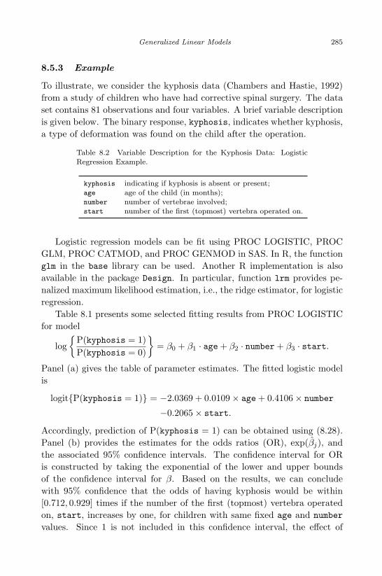
April 29, 2009 11:50 World Scientific Book - 9in x 6in Regression˙master
Generalized Linear Models 285
8.5.3 Example
To illustrate, we consider the kyphosis data (Chambers and Hastie, 1992)from a study of children who have had corrective spinal surgery. The dataset contains 81 observations and four variables. A brief variable descriptionis given below. The binary response, kyphosis, indicates whether kyphosis,a type of deformation was found on the child after the operation.
Table 8.2 Variable Description for the Kyphosis Data: LogisticRegression Example.
kyphosis indicating if kyphosis is absent or present;age age of the child (in months);number number of vertebrae involved;start number of the first (topmost) vertebra operated on.
Logistic regression models can be fit using PROC LOGISTIC, PROCGLM, PROC CATMOD, and PROC GENMOD in SAS. In R, the functionglm in the base library can be used. Another R implementation is alsoavailable in the package Design. In particular, function lrm provides pe-nalized maximum likelihood estimation, i.e., the ridge estimator, for logisticregression.
Table 8.1 presents some selected fitting results from PROC LOGISTICfor model
log
P(kyphosis = 1)P(kyphosis = 0)
= β0 + β1 · age + β2 · number + β3 · start.
Panel (a) gives the table of parameter estimates. The fitted logistic modelis
logitP(kyphosis = 1) = −2.0369 + 0.0109× age + 0.4106× number
−0.2065× start.
Accordingly, prediction of P(kyphosis = 1) can be obtained using (8.28).Panel (b) provides the estimates for the odds ratios (OR), exp(βj), andthe associated 95% confidence intervals. The confidence interval for ORis constructed by taking the exponential of the lower and upper boundsof the confidence interval for β. Based on the results, we can concludewith 95% confidence that the odds of having kyphosis would be within[0.712, 0.929] times if the number of the first (topmost) vertebra operatedon, start, increases by one, for children with same fixed age and number
values. Since 1 is not included in this confidence interval, the effect of

April 29, 2009 11:50 World Scientific Book - 9in x 6in Regression˙master
286 Linear Regression Analysis: Theory and Computing
Table 8.3 Analysis Results for the Kyphosis Data from PROC LOGISTIC.
(a) Analysis of Maximum Likelihood Estimates
Standard WaldParameter DF Estimate Error Chi-Square Pr > ChiSq
Intercept 1 −2.0369 1.4496 1.9744 0.1600Age 1 0.0109 0.00645 2.8748 0.0900
Number 1 0.4106 0.2249 3.3340 0.0679Start 1 −0.2065 0.0677 9.3045 0.0023
(b) Odds Ratio Estimates
Point 95% WaldEffect Estimate Confidence Limits
Age 1.011 0.998 1.024Number 1.508 0.970 2.343Start 0.813 0.712 0.929
(d) Wald Test for H0 : β1 = β2 = 0.
WaldChi-Square DF Pr > ChiSq
5.0422 2 0.0804
(c) Estimated Covariance Matrix
Intercept Age Number Start
Intercept 2.101364 −0.00433 −0.27646 −0.0371Age −0.00433 0.000042 0.000337 −0.00012
Number −0.27646 0.000337 0.050565 0.001681Start −0.0371 −0.00012 0.001681 0.004583
start is significant at α = 0.05, which is consistent with the Wald test inPanel (a). Panel (c) gives an example of the Wald test in its more generalform for testing H0 : β1 = β2 = 0. In this case,
Λ =[
0 1 0 00 0 1 0
]
of rank 2 when applying equation (8.20). The calculation also involvesthe estimated variance-covariance matrix for β, as shown in Panel (d).Referred to χ2(2), the resultant p-value, 0.0804, is rather marginal. Atthe significance level α = 0.05, one might consider dropping both age andnumber from the model.

April 29, 2009 11:50 World Scientific Book - 9in x 6in Regression˙master
Generalized Linear Models 287
8.6 Poisson Regression for Count Data
We next study the loglinear or Poisson models for count data as anotherexample of GLM. Counts are frequencies of some event. Examples includethe number of car accidents in different cities over a given period of time,the number of daily phone calls received in a call center, the number ofstudents graduated from a high school, and so on. Count data are alsocommonly encountered in contingency tables.
8.6.1 The Loglinear Model
The Poisson or log-linear model is a popular GLM for count data, ideallywhen successive events occur independently and at the same rate. When theresponse Yi follows Poisson(µi) for i = 1, . . . , n, its probability distributionfunction is
fYi(yi) = e−µiµyi
i /yi! = exp yi log µi − µi − log yi!
= exp
yiθi − exp(θi)1
+ (− log yi!)
with the natural parameter θi = log(µi). Thus, in exponential family form,b(θi) = exp(θi), a(φ) = 1, and c(yi, φ) = − log(yi!). It follows from (8.3)that
E(Yi) = b′(θi) = exp(θi) = µi
Var(Yi) = b′′(θi) = exp(θi) = µi.
The log-linear model is specified as
log(µi) = ηi = xtiβ for i = 1, . . . , n. (8.31)
The canonical link, i.e., the logarithm function, is applied. In this model,one-unit increase in Xj has a multiplicative impact exp(βj) on the meanresponse, holding other predictors fixed. It is worth mentioning that thelog-linear or Poisson model in (8.31) is different from the ordinary Gaussianlinear model with logarithm transformation on the response
log yi = xtiβ + εi with εi ∼ N(0, σ2).
The log likelihood for the Poisson model (8.31) is given as
L(β) =∑
i
yi log µi −∑
i
µi −∑
i
log yi!.
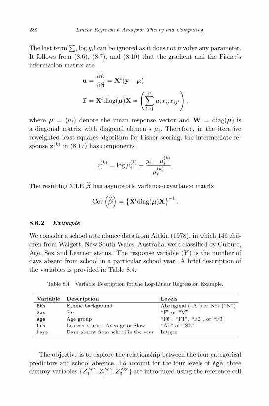
April 29, 2009 11:50 World Scientific Book - 9in x 6in Regression˙master
288 Linear Regression Analysis: Theory and Computing
The last term∑
i log yi! can be ignored as it does not involve any parameter.It follows from (8.6), (8.7), and (8.10) that the gradient and the Fisher’sinformation matrix are
u =∂L
∂β= Xt(y − µ)
I = Xtdiag(µ)X =
(n∑
i=1
µixijxij′
),
where µ = (µi) denote the mean response vector and W = diag(µ) isa diagonal matrix with diagonal elements µi. Therefore, in the iterativereweighted least squares algorithm for Fisher scoring, the intermediate re-sponse z(k) in (8.17) has components
z(k)i = log µ
(k)i +
yi − µ(k)i
µ(k)i
.
The resulting MLE β has asymptotic variance-covariance matrix
Cov(β
)=
Xtdiag(µ)X
−1.
8.6.2 Example
We consider a school attendance data from Aitkin (1978), in which 146 chil-dren from Walgett, New South Wales, Australia, were classified by Culture,Age, Sex and Learner status. The response variable (Y ) is the number ofdays absent from school in a particular school year. A brief description ofthe variables is provided in Table 8.4.
Table 8.4 Variable Description for the Log-Linear Regression Example.
Variable Description Levels
Eth Ethnic background Aboriginal (“A”) or Not (“N”)Sex Sex “F” or “M”Age Age group “F0”, “F1”, “F2”, or “F3”Lrn Learner status: Average or Slow “AL” or “SL”Days Days absent from school in the year Integer
The objective is to explore the relationship between the four categoricalpredictors and school absence. To account for the four levels of Age, threedummy variables Z Age
1 , Z Age2 , Z Age
3 are introduced using the reference cell
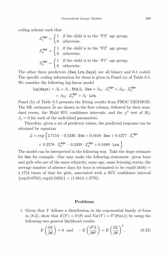
April 29, 2009 11:50 World Scientific Book - 9in x 6in Regression˙master
Generalized Linear Models 289
coding scheme such that
Z Age1 =
1 if the child is in the “F3” age group;0 otherwise.
Z Age2 =
1 if the child is in the “F2” age group;0 otherwise.
Z Age3 =
1 if the child is in the “F1” age group;0 otherwise.
The other three predictors Sex, Lrn, Days are all binary and 0-1 coded.The specific coding information for them is given in Panel (a) of Table 8.5.We consider the following log-linear model
log(days) = β0 + β1 · Ethβ2 · Sex + β31 · Z Age1 + β32 · Z Age
2
+ β33 · Z Age3 + β4 · Lrn.
Panel (b) of Table 8.5 presents the fitting results from PROC GENMOD.The ML estimates βs are shown in the first column, followed by their stan-dard errors, the Wald 95% confidence intervals, and the χ2 test of H0:βj = 0 for each of the individual parameters.
Therefore, given a set of predictor values, the predicted response can beobtained by equation
µ = exp
2.7154− 0.5336 · Eth + 0.1616 · Sex + 0.4277 · Z Age1
+ 0.2578 · Z Age2 − 0.3339 · Z Age
3 + 0.3489 · Lrn.
The model can be interpreted in the following way. Take the slope estimatefor Sex for example. One may make the following statement: given boysand girls who are of the same ethnicity, same age, same learning status, theaverage number of absence days for boys is estimated to be exp(0.1616) =1.1754 times of that for girls, associated with a 95% confidence intervalexp(0.0782), exp(0.2450) = (1.0813, 1.2776).
Problems
1. Given that Y follows a distribution in the exponential family of formin (8.2), show that E(Y ) = b′(θ) and Var(Y ) = b′′(θ)a(φ) by using thefollowing two general likelihood results
E
(∂L
∂θ
)= 0 and − E
(∂2L
∂θ2
)= E
(∂L
∂θ
)2
, (8.32)

April 29, 2009 11:50 World Scientific Book - 9in x 6in Regression˙master
290 Linear Regression Analysis: Theory and Computing
Table 8.5 Analysis Results for the School Absence Data from PROC GENMOD.
(a) Class Level Information
Class Value Design Variables
Eth N 1A 0
Sex M 1F 0
Age F3 1 0 0F2 0 1 0F1 0 0 1F0 0 0 0
Lrn SL 1AL 0
(b) Analysis of Parameter Estimates
Standard Wald 95% Chi-Parameter DF Estimate Error Confidence Limits Square
Intercept 1 2.7154 0.0647 2.5886 2.8422 1762.30Eth N 1 −0.5336 0.0419 −0.6157 −0.4515 162.32Sex M 1 0.1616 0.0425 0.0782 0.2450 14.43Age F3 1 0.4277 0.0677 0.2950 0.5604 39.93
F2 1 0.2578 0.0624 0.1355 0.3802 17.06F1 1 −0.3339 0.0701 −0.4713 −0.1965 22.69
Lrn SL 1 0.3489 0.0520 0.2469 0.4509 44.96
where L(θ, φ) = log fY (y) = yθ − b(θ)/a(φ) + c(y, φ) is the log like-lihood. The two equations in (8.32) hold under some regularity condi-tions given in Sec. 4.8 of Cox and Hinkley (1974).
2. Let y ∼ binomial(n, π). We consider the maximum likelihood basedinference on the parameter π.
(a) Write down the log-likelihood function L(π).(b) Find the score function
u(π) =y
π− n− y
1− πand the Fisher’s information
I(π) =n
π · (1− π).
(c) Find the MLE of π, π. Show that E(π) = π and
Var(π) =π(1− π)
n=
1I(π)
.
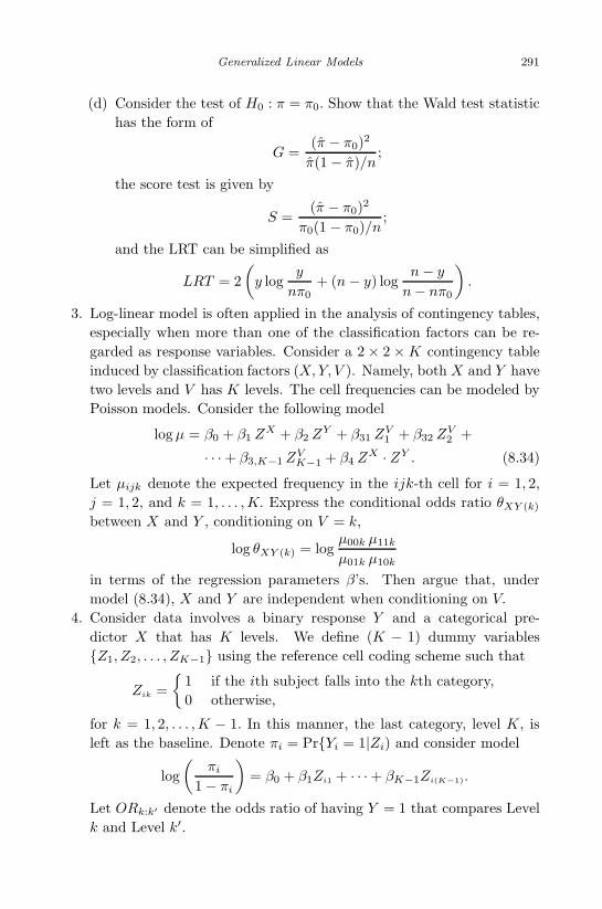
May 7, 2009 10:22 World Scientific Book - 9in x 6in Regression˙master
Generalized Linear Models 291
(d) Consider the test of H0 : π = π0. Show that the Wald test statistichas the form of
G =(π − π0)2
π(1 − π)/n;
the score test is given by
S =(π − π0)2
π0(1 − π0)/n;
and the LRT can be simplified as
LRT = 2(
y logy
nπ0+ (n− y) log
n− y
n− nπ0
).
3. Log-linear model is often applied in the analysis of contingency tables,especially when more than one of the classification factors can be re-garded as response variables. Consider a 2 × 2 ×K contingency tableinduced by classification factors (X, Y, V ). Namely, both X and Y havetwo levels and V has K levels. The cell frequencies can be modeled byPoisson models. Consider the following model
log µ = β0 + β1 ZX + β2 ZY + β31 ZV1 + β32 ZV
2 +
· · ·+ β3,K−1 ZVK−1 + β4 ZX · ZY . (8.34)
Let µijk denote the expected frequency in the ijk-th cell for i = 1, 2,j = 1, 2, and k = 1, . . . , K. Express the conditional odds ratio θXY (k)
between X and Y , conditioning on V = k,
log θXY (k) = logµ00k µ11k
µ01k µ10k
in terms of the regression parameters β’s. Then argue that, undermodel (8.34), X and Y are independent when conditioning on V.
4. Consider data involves a binary response Y and a categorical pre-dictor X that has K levels. We define (K − 1) dummy variablesZ1, Z2, . . . , ZK−1 using the reference cell coding scheme such that
Zik =
1 if the ith subject falls into the kth category,0 otherwise,
for k = 1, 2, . . . , K − 1. In this manner, the last category, level K, isleft as the baseline. Denote πi = PrYi = 1|Zi) and consider model
log(
πi
1− πi
)= β0 + β1Zi1 + · · ·+ βK−1Zi(K−1).
Let ORk:k′ denote the odds ratio of having Y = 1 that compares Levelk and Level k′.
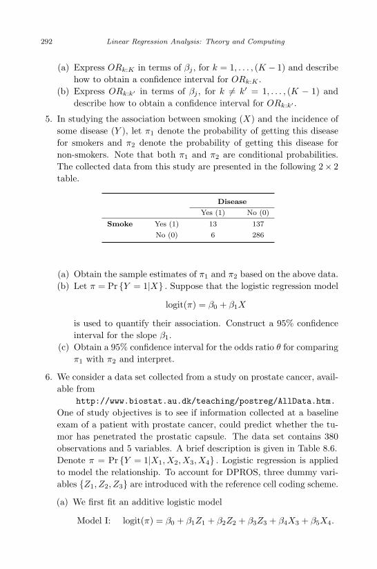
April 29, 2009 11:50 World Scientific Book - 9in x 6in Regression˙master
292 Linear Regression Analysis: Theory and Computing
(a) Express ORk:K in terms of βj , for k = 1, . . . , (K − 1) and describehow to obtain a confidence interval for ORk:K .
(b) Express ORk:k′ in terms of βj , for k 6= k′ = 1, . . . , (K − 1) anddescribe how to obtain a confidence interval for ORk:k′ .
5. In studying the association between smoking (X) and the incidence ofsome disease (Y ), let π1 denote the probability of getting this diseasefor smokers and π2 denote the probability of getting this disease fornon-smokers. Note that both π1 and π2 are conditional probabilities.The collected data from this study are presented in the following 2× 2table.
Disease
Yes (1) No (0)
Smoke Yes (1) 13 137
No (0) 6 286
(a) Obtain the sample estimates of π1 and π2 based on the above data.(b) Let π = Pr Y = 1|X . Suppose that the logistic regression model
logit(π) = β0 + β1X
is used to quantify their association. Construct a 95% confidenceinterval for the slope β1.
(c) Obtain a 95% confidence interval for the odds ratio θ for comparingπ1 with π2 and interpret.
6. We consider a data set collected from a study on prostate cancer, avail-able from
http://www.biostat.au.dk/teaching/postreg/AllData.htm.
One of study objectives is to see if information collected at a baselineexam of a patient with prostate cancer, could predict whether the tu-mor has penetrated the prostatic capsule. The data set contains 380observations and 5 variables. A brief description is given in Table 8.6.Denote π = Pr Y = 1|X1, X2, X3, X4 . Logistic regression is appliedto model the relationship. To account for DPROS, three dummy vari-ables Z1, Z2, Z3 are introduced with the reference cell coding scheme.
(a) We first fit an additive logistic model
Model I: logit(π) = β0 + β1Z1 + β2Z2 + β3Z3 + β4X3 + β5X4.

April 29, 2009 11:50 World Scientific Book - 9in x 6in Regression˙master
Generalized Linear Models 293
Table 8.6 Variable Description for the Prostate Cancer Data.
Var Name Description Type Values
Y CAPSULE Tumor penetration of prostatic capsule binary 0 - no penetration
1 - penetration
X1 AGE Age in years continuous 32 distinct values
X2 DPROS Results of the digital rectal exam categorical 1 No Nodule
2 Unilobar Nodule (Left)
3 Unilobar Nodule (Right)
4 Bilobar Nodule
X3 DCAPS Detection of capsular involvement in binary 1 - No
rectal exam 0 - Yes
X4 PSA Prostatic Specific Antigen Value mg/ml continuous 211 distinct values
Provided in Table 8.7 are some of ML fitting results from SASPROC LOGISTIC. Answer the following question(s) based onModel I.
i. Suppose that there are two individuals, A and B, both havingdetection of capsular involvement (DCAPS, X3) but no nodule(DPROS, X2) found in the rectal exam. Patient A has a PSAvalue of 10 mg/ml higher than Patient B. Obtain a point estimateof the odds ratio for having tumor penetration that compares Aversus B. Construct a Wald 95% confidence interval for this oddsratio.
ii. Given an individual who has detection of capsular involvement(DCAPS, X3) but no nodule (DPROS, X2) found in the rectalexam and a PSA value of 20 mg/ml, apply Model I to predictthe probability for this individual to have tumor penetration ofprostatic capsule. Construct a Wald 95% confidence interval forthis probability.
(b) Next, we consider an interaction model
Model II: logit(π) = β0+β1Z1+β2Z2+β3Z3+β4X3+β5X4+β6X3·X4.
Provided in Table 8.8 are some of ML fitting results from SASPROC LOGISTIC. Answer the following question(s) based onModel II.
i. Suppose that there are two individuals, A and B, both havingdetection of capsular involvement (DCAPS, X3) but no nodule

April 29, 2009 11:50 World Scientific Book - 9in x 6in Regression˙master
294 Linear Regression Analysis: Theory and Computing
Table 8.7 Table of Parameter Estimates and the EstimatedCovariance Matrix for Model I: the Prostate Cancer Data.
(a) Analysis of Maximum Likelihood Estimates
Standard Wald
Parameter DF Estimate Error Chi-Square Pr > ChiSq
Intercept 1 0.4069 0.5144 0.6258 0.4289
DPROS 3 1 0.0977 0.3970 0.0605 0.8056
DPROS 2 1 −0.5910 0.3855 2.3503 0.1253
DPROS 1 1 −1.5724 0.4293 13.4169 0.0002
DCAPS 1 −1.0309 0.4284 5.7899 0.0161
PSA 1 0.0468 0.00967 23.4280 < .0001
(b) Estimated Covariance Matrix for β.
DPROS DPROS DPROS
Intercept 3 2 1 DCAPS PSA
Intercept 0.2646 −0.10357 −0.09627 −0.06 −0.1561 −0.00182
DPROS 3 −0.1036 0.15762 0.11179 0.10964 −0.0150 0.00051
DPROS 2 −0.0963 0.11179 0.14864 0.11032 −0.0212 0.00036
DPROS 1 −0.0899 0.10964 0.11032 0.18429 −0.0216 −0.00001
DCAPS −0.1561 −0.01502 −0.02117 −0.02156 0.1836 0.00038
PSA −0.0018 0.00051 0.00036 −0.00001 0.0004 0.00009
(DPROS, X2) found in the rectal exam. A has a PSA score of10 mg/ml higher than B. Obtain a point estimate of the oddsratio for having tumor penetration that compares A versus B.Construct a Wald 95% confidence interval for this odds ratio.
7. Table 8.9 presents minus two times of the maximized log-likelihoodscore for several candidate models for the prostate cancer data.
i. Compute the AIC and BIC for each of the above models. Basedon these two criteria, which one is the best?
ii. Concerning Model I, use the likelihood ratio test to see at signif-icance level α = 0.05 if the categorical predictor DPROS (X2)can be dropped.

May 8, 2009 15:56 World Scientific Book - 9in x 6in Regression˙master
Generalized Linear Models 295
Table 8.8 Table of Parameter Estimates and the Estimated Covariance Matrix forModel II: the Prostate Cancer Data.
(a) Analysis of Maximum Likelihood Estimates
Standard Wald
Parameter DF Estimate Error Chi-Square Pr > ChiSq
Intercept 1 1.0626 0.6222 2.9163 0.0877
DPROS 3 1 0.0667 0.3982 0.0280 0.8670
DPROS 2 1 −0.6133 0.3854 2.5321 0.1116
DPROS 1 1 −1.6477 0.4353 14.3295 0.0002
DCAPS 1 −1.7478 0.5787 9.1221 0.0025
PSA 1 0.0149 0.0164 0.8187 0.3656
DCAPS*PSA 1 0.0397 0.0198 4.0215 0.0449
(b) Estimated Covariance Matrix for β
DPROS DPROS DPROS
Intercept 3 2 1 DCAPS PSA DCAPSPSA
Intercept 0.387192 −0.10879 −0.1008 −0.10779 −0.29216 −0.00696 0.006791
DPROS 3 −0.10879 0.158585 0.111772 0.110618 −0.00932 0.000783 −0.00037
DPROS 2 −0.1008 0.111772 0.14857 0.110755 −0.01573 0.000581 −0.0003
DPROS 1 −0.10779 0.110618 0.110755 0.189455 −0.00201 0.000847 −0.0011
DCAPS −0.29216 −0.00932 −0.01573 −0.00201 0.334893 0.006327 −0.00782
PSA −0.00696 0.000783 0.000581 0.000847 0.006327 0.00027 −0.00027
DCAPSPSA 0.006791 −0.00037 −0.0003 −0.0011 −0.00782 −0.00027 0.000392
Table 8.9 The Maximized Loglikelihood Scores for Several Fitted Models with the Prostate CancerData.
Model Form −2 log L AIC BIC
I logit(π) = β0 + β1Z1 + β2Z2 + β3Z3 + β4X3 + β5X4 424.018 (1) (2)
II logit(π) = β0 + β1Z1 + β2Z2 + β3Z3 + β4X3 + β5X4 + β6X3 · X4. 420.897 (3) (4)
III logit(π) = β0 + β1X1 + β2Z1 + β3Z2 + β4Z3 + β5X3 + β6X4 423.964 (5) (6)
IV logit(π) = β0 + β1X3 + β2X4 452.461 (7) (8)

April 29, 2009 11:50 World Scientific Book - 9in x 6in Regression˙master
This page intentionally left blankThis page intentionally left blank
April 29, 2009 11:50 World Scientific Book - 9in x 6in Regression˙master
Chapter 9
Bayesian Linear Regression
The Bayesian approach, offering different viewpoints towards statisticalmodeling, takes additional or historical evidences into account of the in-ference and analysis of current data. The advances in Bayesian statisticshave been innovative and fruitful in both theories and computation overdecades. In this chapter, we shall discuss the Bayesian approaches com-monly used in linear regression. In order to miss small, we shall aim smallin our coverage of this topic. Specifically we first discuss Bayesian linearmodels with conjugate normal-gamma priors. Then we discuss a relativelynew development, Bayesian model averaging (BMA), for model selectionand evaluation.
9.1 Bayesian Linear Models
9.1.1 Bayesian Inference in General
There are two main streams of viewpoints and approaches in statistics, un-derlaid respectively by the Fisherian and the Bayesian philosophies. So farwe have mainly followed the Fisherian approach, named after Sir RonaldFisher, to present the linear regression techniques. One key feature in thisparadigm is that the regression coefficients in β and the error varianceσ2 are considered as fixed parameters or unknown constants. Thereforeconcepts such as unbiased estimators, hypothesis testing, confidence inter-vals, etc. follow. The Fisherian inference is often combined with likelihoodmethods. On the other hand, the Bayesian philosophy, named after theReverend Thomas Bayes, allows for parameters to be treated as randomvariables as well, under the premise that all uncertainties should be prob-abilistically modelled. An important advantage for doing so is to facilitate
297

April 29, 2009 11:50 World Scientific Book - 9in x 6in Regression˙master
298 Linear Regression Analysis: Theory and Computing
incorporation of prior knowledge and beliefs from scientific field expertsand information from historic studies into the inference and analysis. TheBayesian approach involves concepts such as prior, posterior distributions,and Bayes estimation or decision rules. One is referred to Berger (1993) fora full account of Bayesian inference.
The main idea of the Bayesian analysis is outlined in the following.In Bayesian approach, all information or uncertainties are integrated withvarious types of distribution functions, from which inference and conclusionare then made, obeying the laws of probability theories such as Bayes’ rule.Let D be a generic notation for the observed data. To draw conclusionson parameter vector θ of interest, the Bayesian inference is based on its itsconditional distribution conditioning on D, i.e., the posterior distribution,given by
f(θ|D) =f(θ, D)f(D)
, (9.1)
where f(θ, D) is the joint density of D and θ and f(D) is the marginaldensity of D. With slight abuse of notations, we have used f(·) as a genericsymbol for all density functions for the sake of convenience. Applying theBayes’ rule, we have
f(θ, D) = f(D|θ)f(θ), (9.2)
where f(D|θ) is the conditional density of D given θ, i.e., the likelihoodfunction, and f(θ) is the prior density of θ which integrates prior beliefsabout θ. The marginal density of D, f(D), can be obtained by integratingθ out of f(θ, D). Thus, the posterior distribution in (9.1) becomes
f(θ|D) =f(D|θ)f(θ)
f(D)
=f(D|θ)f(θ)∫
Ωf(D|θ)f(θ)dθ
= c · f(D|θ)f(θ)
∝ f(D|θ)f(θ), (9.3)
where Ω denotes the range of θ; the notation ∝ means “up to a constant”;and the normalizing constant c =
∫Ω
f(D|θ)f(θ)dθ, which ensures thatf(θ|D) is a valid density function satisfying
∫Ω
f(θ|D)dθ = 1, does not in-volve θ. Point estimates and confidence intervals of θ can then be obtainedfrom the joint posterior density f(θ|D) and its associated marginal poste-riors f(θj |D) for each component θj of θ. A marginal posterior f(θj |D) isderived by integrating other components out of the joint posterior f(θ|D).

April 29, 2009 11:50 World Scientific Book - 9in x 6in Regression˙master
Bayesian Linear Regression 299
As opposed to likelihood optimization in the Fisherian approach,Bayesian computation essentially involves derivations of assorted proba-bility distributions by solving integrals. The difficulty level of a Bayesiananalysis depends on prior specification besides many other aspects. Some-times, a prior is chosen for mathematical convenience to have easily solv-able integrals. Conjugate priors, for instance, result in posteriors from thesame family. Most often, the integrals involved are complicated or even in-tractable. In this case, approximations of multiple integration can be madeeither analytically by techniques such as Laplace transforms or computa-tionally by numerical integration. One is referred to Bayesian texts, e.g.,Tanner (1998) and Carlin and Louis (2000), for detailed implementationand computation issues in Bayesian analysis.
9.1.2 Conjugate Normal-Gamma Priors
We now discuss the Bayesian approach for fitting normal linear regressionmodels given by y ∼ N
Xβ, σ2I, with X being n× (k+1) of full column
rank (k +1). We first reparametrize the model by introducing the precisionparameter ν = 1/σ2. Then the likelihood function can be written as, up toa constant
L(β, σ2) = f(y|β, ν) ∝ νn/2 exp−ν · (y −Xβ)t(y −Xβ)/2
. (9.4)
To seek conjugate priors that yields posteriors of similar functional form,we rewrite the likelihood so that terms involving β are in a multivariatenormal density function form. Using
(y −Xβ)t(y −Xβ) = (y −Xβ)t(y −Xβ) + (β − β)t(XtX)(β − β)
= n− (k + 1) · σ2 + (β − β)t(XtX)(β − β),
the likelihood in (9.4) can be expressed as
f(y|β, ν) ∝
νn−(k+1)
2 exp(−n− (k + 1)σ2
2ν
)
×
νk+12 exp
(− (β − β)t(ν ·XtX)(β − β)
2
). (9.5)
It has two parts: the first part contains a kernel of a
Γ
n− (k + 1)2
− 1,n− (k + 1)σ2
2
density for ν and the second part contains a kernel of a multivariate normalN
(β, (ν ·XtX)−1
)distribution for β.

April 29, 2009 11:50 World Scientific Book - 9in x 6in Regression˙master
300 Linear Regression Analysis: Theory and Computing
In general, a positive random variable U follows a Γ(a, b) distributionwith a shape parameter a > 0 and a rate parameter b > 0, i.e., U ∼ Γ(a, b),if its density is given by
f(u; a, b) =ba
Γ(a)ua−1e−bu, (9.6)
where Γ(a) =∫∞0
ua−1e−udu is the Gamma function. Alternatively, thescale parameter 1/b can be used to express the gamma density (9.6). GivenU ∼ Γ(a, b), we have
E(U) =a
band Var(U) =
a
b2.
The inverse of U , 1/U , is said to follow the inverse Gamma distributionwith mean and variance given by
E(1/U) =b
a− 1and Var(1/U) =
b2
(a− 1)2(a− 2). (9.7)
Note that in (9.5), the multivariate normal distri-bution N
(β, (ν ·XtX)−1
)for β depends on ν. This suggests a natural
choice for the priors of form
f(β, ν) = f(β|ν)f(ν),
where ν ∼ Γ(a, b) with density f(ν) given as in (9.6); β|ν ∼ N(β0,V/ν)with density
f(β|ν) = ν(k+1)/2 exp−ν · (β − β0)
tV−1(β − β0)/2
; (9.8)
and the quantities (a, b, β0,V) are the so-called super-parameters.To summarize, the Bayesian linear regression model we shall consider
has the following specification:
y|(β, ν) ∼ N(Xβ, I/ν)β|ν ∼ Nk+1(β0, V/ν)ν ∼ Γ(a, b).
(9.9)
Under this model, the posterior joint density f(β, ν|y) is, using (9.4), (9.6),and (9.8),
f(β, ν|y) ∝ f(y|β, ν)f(β|ν)f(ν) (9.10)
∝ ν(n+2a+k+1)/2−1 exp[−(ν/2) · 2b + (β − β0)
tV−1(β − β0)
+ (y −Xβ)t(y −Xβ)]
(9.11)
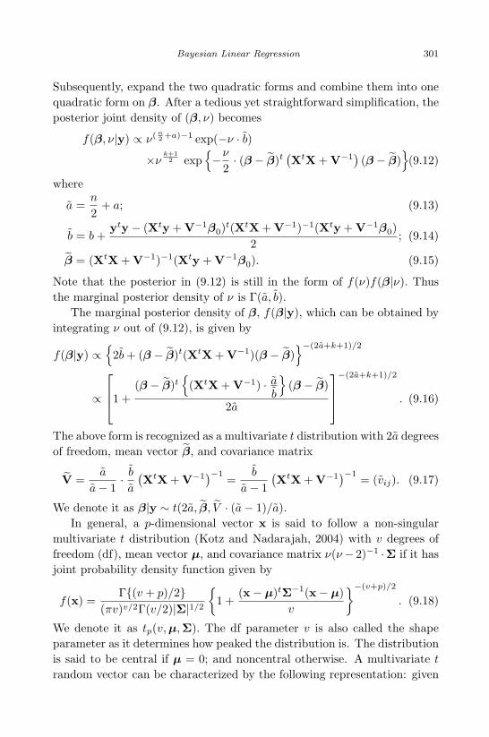
April 29, 2009 11:50 World Scientific Book - 9in x 6in Regression˙master
Bayesian Linear Regression 301
Subsequently, expand the two quadratic forms and combine them into onequadratic form on β. After a tedious yet straightforward simplification, theposterior joint density of (β, ν) becomes
f(β, ν|y) ∝ ν( n2 +a)−1 exp(−ν · b)
×νk+12 exp
−ν
2· (β − β)t
(XtX + V−1
)(β − β)
(9.12)
where
a =n
2+ a; (9.13)
b = b +yty − (Xty + V−1β0)t(XtX + V−1)−1(Xty + V−1β0)
2; (9.14)
β = (XtX + V−1)−1(Xty + V−1β0). (9.15)
Note that the posterior in (9.12) is still in the form of f(ν)f(β|ν). Thusthe marginal posterior density of ν is Γ(a, b).
The marginal posterior density of β, f(β|y), which can be obtained byintegrating ν out of (9.12), is given by
f(β|y) ∝
2b + (β − β)t(XtX + V−1)(β − β)−(2a+k+1)/2
∝
1 +
(β − β)t
(XtX + V−1) · ab
(β − β)
2a
−(2a+k+1)/2
. (9.16)
The above form is recognized as a multivariate t distribution with 2a degreesof freedom, mean vector β, and covariance matrix
V =a
a− 1· b
a
(XtX + V−1
)−1=
b
a− 1(XtX + V−1
)−1= (vij). (9.17)
We denote it as β|y ∼ t(2a, β, V · (a− 1)/a).In general, a p-dimensional vector x is said to follow a non-singular
multivariate t distribution (Kotz and Nadarajah, 2004) with v degrees offreedom (df), mean vector µ, and covariance matrix ν(ν− 2)−1 ·Σ if it hasjoint probability density function given by
f(x) =Γ(v + p)/2
(πv)v/2Γ(v/2)|Σ|1/2
1 +
(x− µ)tΣ−1(x− µ)v
−(v+p)/2
. (9.18)
We denote it as tp(v, µ,Σ). The df parameter v is also called the shapeparameter as it determines how peaked the distribution is. The distributionis said to be central if µ = 0; and noncentral otherwise. A multivariate t
random vector can be characterized by the following representation: given

April 29, 2009 11:50 World Scientific Book - 9in x 6in Regression˙master
302 Linear Regression Analysis: Theory and Computing
that y ∼ Np(µ,Σ) is independent of v · s2 ∼ χ2(v), if we define x = y/s,then x ∼ tp(v,µ,Σ). With this representation, it follows an importantproperty (Lin, 1971) that,
x ∼ tp(v, µ,Σ) ⇐⇒ at(x− µ)√atΣa
∼ t(v) (9.19)
for any p-dimensional nonzero vector a. This property is useful in statisticalinference about β.
9.1.3 Inference in Bayesian Linear Model
The posterior mean can be used as the Bayesian point estimator. Sinceβ|y ∼ t(2a, β, V · (a− 1)/a), the Bayesian estimate of β in model (9.9) is
β = (XtX + V−1)−1(Xty + V−1β0) = (βj) (9.20)
as also given by (9.15). It is interesting to note that β can be obtained asthe generalized least squares estimator (see Section 7.2) of β in the followingaugmented linear model:
(yβ0
)=
(X
Ik+1
)β +
(ε
ε0
), where
(ε
ε0
)∼ N
(I OO V
). (9.21)
The implication is that the prior information on β can be integrated intothe least squares estimation by adding some pseudo-data.
Two special cases are worth noting. The first situation, correspondingto noninformative priors, is when β0 = 0, a = b ≈ 0, and V−1 ≈ O. In thiscase, it can be easily verified that 2b ≈ SSE = yty−ytX(XtX)−1Xty anda = n/2. Thus the posterior mean vector and covariance matrix of β are
β ≈ (XtX)−1Xty
V ≈ SSE
n− 2(XtX)−1,
which are similar to their counterparts in ordinary LS estimation. Thesecond case is when β0 = 0 and V−1 = λI for some constant λ > 0. It canbe seen that the Bayesian point estimator of β becomes
β = (XtX + λI)−1Xty, (9.22)
a form known as the ridge or shrinkage estimator. The ridge or shrinkageestimator is initially proposed as a remedial measure for handling the mul-ticollinearity problem encountered in linear regression. We shall furtherexplore it in Section 7.3.

April 29, 2009 11:50 World Scientific Book - 9in x 6in Regression˙master
Bayesian Linear Regression 303
Interval inference and hypothesis testing about β and its componentscan be derived from property (9.19). The posterior distribution of a linearcombination on β is a t distribution with df 2a = n + 2a, i.e.,
atβ − atβ
atVa
∣∣∣∣∣y ∼ t(n + 2a), (9.23)
where β and V are given in (9.20) and (9.17). In particular, the posteriordistribution of βj is
βj − βj
vjj
∣∣∣∣∣y ∼ t(n + 2a). (9.24)
A 100× (1− α)% Bayesian confidence interval for βj can be given as
βj ± t(1− α/2, n + 2a) · vjj , (9.25)
where t(1 − α/2, n + 2a) denotes the (1 − α/2) × 100-th percentile of thet(n+2a) distribution. Since β’s are random variables in Bayesian inference,it is simply and correctly safe to state that, with (1−α) probability, βj fallsinto the (1−α)×100% Bayesian confidence interval. Recall that in classicalinference one has to be careful not to interpret confidence intervals in sucha manner. Clearly, equation (9.23) can also be useful in Bayesian intervalestimation of the expected response E(yp) = xt
pβ at any given predictorvector x = xp.
In addition, since ν|y ∼ Γ(a, b) where a and b are given in (9.13) and(9.14), the posterior distribution of σ2 = 1/ν is an inverse Gamma distri-bution. Using (9.7), a Bayesian point estimator of σ2 is the posterior meanb/(a− 1), i.e.,
σ2 =b +
yty − (Xty + V−1β0)t(XtX + V−1)−1(Xty + V−1β0)
/2
n/2 + a− 1.
A (1−α)×100% Bayesian confidence interval for σ2 can also be constructedusing percentiles from the inverse Gamma distribution.
9.1.4 Bayesian Inference via MCMC
More often the marginal posterior density function for a parameter of in-terest is not explicitly available in Bayesian analysis. In this case, thesolutions are provided by Markov Chain Monte Carlo (MCMC) simulationmethods. The Monte Carlo methods, traced back to Metropolis and Ulam(1949) and then extensively studied and expanded by many others, are a

April 29, 2009 11:50 World Scientific Book - 9in x 6in Regression˙master
304 Linear Regression Analysis: Theory and Computing
very general class of computational methods that perform complicated cal-culations, most notably those involving integration and optimization, byusing repetitive random number generation. The Markov chain is referredto a stochastic process or a sequence of random variables, say, X1, X2, . . . ,
that satisfies the Markov property
Pr(Xm+1 ∈ A|X1, . . . , Xm) = Pr(Xm+1 ∈ A|Xm). (9.26)
Namely, the distribution of the random variable at any state of the pro-cess only depends on the random variable at the immediately precedingstep. In other words, the description of the present state fully captures allthe information that could influence the future evolution of the process.The Markov property in (9.26) can be viewed as a generalization of theconcept of independence. Samples obtained from MCMC can be used toapproximate distributions or to compute integrals such as expected values.The ergodic theory states that, under some mild regularity conditions, theMarkov chain process satisfies
limM→∞
1M
M∑m=1
h(Xm) = Eh(X). (9.27)
The MCMC methods have fundamental use in many, if not all, scientificfields and encompass a prohibitively long list of related references in theliterature. In Bayesian analysis, MCMC methods provide empirical realiza-tion and exploration of posterior distributions especially when their closedforms are not easily available.
While a few different ways to perform MCMC in Bayesian linear regres-sion are available, we describe a very popular algorithm, called the Gibbssampler or Gibbs sampling. Gibbs sampler, as a special case of the MCMCmethods, is particularly useful when the conditional posterior distributionof each parameter is explicitly known. The idea of Gibbs sampler is toalternate a sequence of random draws from conditional distributions toeventually characterize the joint distribution of interest.
Consider the Bayesian linear model with specification given by (9.9).From the joint posterior density f(β, ν|y) in (9.12), it can be seen that theconditional posterior density of (β|ν,y) is multivariate normal with meanβ and covariance matrix ν−1(XtX + V−1)−1, i.e.,
β|(ν,y) ∼ Nk+1
β, ν−1(XtX + V−1)−1
. (9.28)
The conditional posterior density of (ν|β,y) is
f(ν|β,y) ∝ νa1−1 exp(−ν × b1),

April 29, 2009 11:50 World Scientific Book - 9in x 6in Regression˙master
Bayesian Linear Regression 305
where
a1 =n + k + 1
2+ a, (9.29)
b1 = b +(β − β)t
(XtX + V−1
)(β − β)
2. (9.30)
That is, ν|(β,y) ∼ Γ(a1, b1).
Algorithm 9.1: Gibbas Sampler for Bayesian Linear Regression.
• Set β(0) = β, the ordinary LSE of β;
• Do m = 1 to M ,
– Given β = β(m−1), generate ν(m) ∼ Γ(a1, b1);
– Given ν = ν(m), generate β(m) ∼ Nk+1
β, ν−1(XtX + V−1)−1
;
– (Optional) Prediction at xp: Generate y(m) ∼ N(xtpβ(m), ν−1
(m));
• End do;
• Burn-In: Throw away the first N0 observations of (β(m), ν(m)).
The Gibbas sampler is outlined in the above algorithm. In the com-putation, β0 and V are super-parameters pre-specified by the user andβ is given in (9.20). Since each draw is always conditional on the pastdraw, the resultant sample is a Markov chain sequence. The very last stepof discarding a few initial observations, known as the “burn-in” strategy,ensures a purer MCMC sample from the posterior densities and leads toimproved performance. Once an MCMC sample (with large M) is availablefor (β, ν), all their inferential properties can be obtained empirically. Forexample, the bounds of confidence intervals for βj ’s can be simply found asappropriate percentiles from the corresponding MCMC sample values.
Note that prior specification plays a critical role in Bayesian analysis.It is often emphasized that priors should reflect a reasonable approxima-tion of the actual information and those developed by statisticians shouldalways refer to experts for validation. The natural normal-gamma conju-gate prior, which has been chosen mainly for mathematical convenience,also has considerable flexibilities to reflect expert prior knowledge on theparameters. For example, these prior distributions could be devised withsmall variances to have strong influence on the posteriors. They could alsobe formulated with large variances so as to have little effect on the posterior
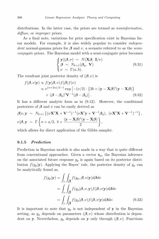
April 29, 2009 11:50 World Scientific Book - 9in x 6in Regression˙master
306 Linear Regression Analysis: Theory and Computing
distributions. In the latter case, the priors are termed as noninformative,diffuse, or improper priors.
As a final note, variations for prior specification exist in Bayesian lin-ear models. For example, it is also widely popular to consider indepen-dent normal-gamma priors for β and ν, a scenario referred to as the semi-conjugate priors. The Bayesian model with a semi-conjugate prior becomes
y|(β, ν) ∼ N(Xβ, I/ν)β ∼ Nk+1(β0, V)ν ∼ Γ(a, b).
(9.31)
The resultant joint posterior density of (β, ν) is
f(β, ν|y) ∝ f(y|β, ν)f(β)f(ν)
∝ ν(n+2a)/2−1 exp[−(ν/2) · 2b + (y −Xβ)t(y −Xβ)
+ (β − β0)tV−1(β − β0)
]. (9.32)
It has a different analytic form as in (9.12). However, the conditionalposteriors of β and ν can be easily derived as
β|ν,y ∼ Nk+1
(νXtX + V−1)−1(νXty + V−1β0), (νXtX + V−1)−1
,
ν|β,y ∼ Γ
n + a/2, b +(y −Xβ)t(y −Xβ)
2
,
which allows for direct application of the Gibbs sampler.
9.1.5 Prediction
Prediction in Bayesian models is also made in a way that is quite differentfrom conventional approaches. Given a vector xp, the Bayesian inferenceon the associated future response yp is again based on its posterior distri-bution f(yp|y). Applying the Bayes’ rule, the posterior density of yp canbe analytically found as,
f(yp|y) =∫
ν
∫
βf(yp,β, ν|y)dβdν
=∫
ν
∫
βf(yp|β, ν,y)f(β, ν|y)dβdν
=∫
ν
∫
βf(yp|β, ν)f(β, ν|y)dβdν. (9.33)
It is important to note that yp is not independent of y in the Bayesiansetting, as yp depends on parameters (β, ν) whose distribution is depen-dent on y. Nevertheless, yp depends on y only through (β, ν). Functions

April 29, 2009 11:50 World Scientific Book - 9in x 6in Regression˙master
Bayesian Linear Regression 307
f(yp|β, ν) and f(β, ν|y) in equation (9.33) can be obtained using
yp|β, ν ∼ N(xtpβ, ν−1), (9.34)
and the Bayesian linear model specification in (9.9). However, the inte-grations involved in (9.33) are still difficult to solve. Comparatively, it ismore convenient to base the inference of yp on Gibbs sampler, as outlinedin Algorithm 9.1.
Table 9.1 Bayesian Linear Regression Results With the Shingle Data.
Least Squares Estimation Bayesian Analysis
Estimate 95% CI Estimate 95% CI
β0 5.656147 4.777982 6.534312 5.656913 4.762665 6.548519
β1 −0.060878 −0.122139 0.000382 −0.060839 −0.122124 0.001082
β2 0.024041 0.014840 0.033242 0.024087 0.014737 0.033405
β3 −0.159635 −0.211159 −0.108110 −0.159749 −0.211082 −0.107679
β4 −0.013595 −0.040586 0.013397 −0.013858 −0.039959 0.013536
σ2 0.038055 0.018579 0.117201 0.047764 0.018721 0.118779
9.1.6 Example
Implementation of Bayesian linear models techniques is available in bothSAS (PROC MCMC and the BAYES statement in PROC GENMOD) andR (several packages available).
To illustrate, we analyze the shingle sales data in Table 4.1. The Rpackage MCMCpack, which implements Bayesian linear regression with semi-conjugate priors in model (9.31), is used for analysis. A logarithm trans-formation is first applied to the response Y. Here we employ a set of non-informative priors with the default specification
β0 = 0, V ≈ O, a = 0.0005, and b = 0.0005.
Gibbs sampler is used to generate 10, 000 MC observations after a “burn-in”of the first N0 = 1, 000 random draws.
Figure 9.1 plots the resultant marginal densities for regression coeffi-cients (β0, β1, . . . , β4) and σ2, obtained by smoothing the empirical densityof the MC samples. Table 9.1 shows the Bayesian estimate together withtheir 95% confidence intervals, which are very similar to the results from LS.This comes as no surprise considering the noninformative priors employed.
We next consider prediction at xp = (1, 5.20, 47.07, 8.87, 8.93)t, whichcorresponds to sample averages of (x0 = 1, x1, x2, x3, x4). To do so, a MC

April 29, 2009 11:50 World Scientific Book - 9in x 6in Regression˙master
308 Linear Regression Analysis: Theory and Computing
3 4 5 6 7 8 9
0.0
0.2
0.4
0.6
0.8
1.0
N = 10000 Bandwidth = 0.06824
Density of (Intercept)
−0.2 −0.1 0.0 0.1
02
46
81
01
21
4
N = 10000 Bandwidth = 0.004781
Density of x1
0.00 0.01 0.02 0.03 0.04 0.05
02
04
06
08
0
N = 10000 Bandwidth = 0.0007307
Density of x2
−0.35 −0.25 −0.15 −0.05
05
10
15
N = 10000 Bandwidth = 0.004005
Density of x3
−0.10 −0.05 0.00 0.05 0.10
05
10
15
20
25
30
N = 10000 Bandwidth = 0.002105
Density of x4
0.0 0.1 0.2 0.3 0.4 0.5 0.6
05
10
15
20
25
N = 10000 Bandwidth = 0.003236
Density of sigma2
Fig. 9.1 Posterior Marginal Densities of (β, σ2): Bayesian Linear Regression for ShingleData.
sample for yp can be formed by computing xtpβ(m), where β(m) denotes the
m-th observation of β in the MC sample. Figure 9.2 plots the posterior den-sity of yp. Based on the MC sample for yp, the point estimate for predictionis the sample mean, 4.934. The 95% prediction interval is (4.823, 5.046),
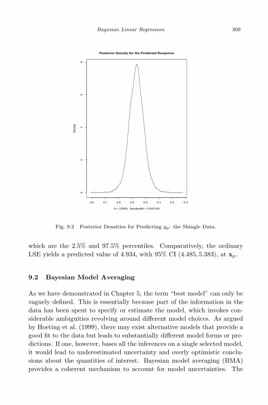
April 29, 2009 11:50 World Scientific Book - 9in x 6in Regression˙master
Bayesian Linear Regression 309
4.6 4.7 4.8 4.9 5.0 5.1 5.2 5.3
02
46
8
Posterior Density for the Predicted Response
N = 10000 Bandwidth = 0.007542
Den
sity
Fig. 9.2 Posterior Densities for Predicting yp: the Shingle Data.
which are the 2.5% and 97.5% percentiles. Comparatively, the ordinaryLSE yields a predicted value of 4.934, with 95% CI (4.485, 5.383), at xp.
9.2 Bayesian Model Averaging
As we have demonstrated in Chapter 5, the term “best model” can only bevaguely defined. This is essentially because part of the information in thedata has been spent to specify or estimate the model, which invokes con-siderable ambiguities revolving around different model choices. As arguedby Hoeting et al. (1999), there may exist alternative models that provide agood fit to the data but leads to substantially different model forms or pre-dictions. If one, however, bases all the inferences on a single selected model,it would lead to underestimated uncertainty and overly optimistic conclu-sions about the quantities of interest. Bayesian model averaging (BMA)provides a coherent mechanism to account for model uncertainties. The

April 29, 2009 11:50 World Scientific Book - 9in x 6in Regression˙master
310 Linear Regression Analysis: Theory and Computing
philosophy underlying BMA is to integrate the information from those rea-sonable models together in an effort to provide a more comprehensive as-sessment and a better understanding of the problems under study. Notethat BMA is not meant to do model ensemble or have combined predictions,a common wrong impression carried by the term ‘model averaging’.
The original idea of BMA can be traced back to the proposal of Leamer(1978). Let M = M1, . . . , MK be the set of all models under considera-tion. Let ∆ denote some quantity that is of central interest to the inference,such as a parameter or a future observation, then its posterior distributiongiven data D is
pr(∆|D) =K∑
k=1
pr(∆|Mk, D)pr(Mk|D), (9.35)
which is an average of the posterior distributions under each of the mod-els, weighted by the posterior model probabilities. The posterior modelprobability of Mk can be computed as
pr(Mk|D) =pr(D|Mk)pr(Mk)∑Kl=1 pr(D|Ml)pr(Ml)
, (9.36)
where
pr(D|Mk) =∫
pr(D|βk,Mk)pr(βk|Mk)dβk (9.37)
is the integrated marginal likelihood of model Mk; βk is the parametersinvolved in Mk; pr(βk|Mk) is the prior distribution of βk; pr(D|βk,Mk) isthe likelihood; and pr(Mk) is the prior model probability that Mk is thetrue model. Define the Bayes factor, B21, for a model M2 against anothermodel M1 given data D to be the ratio of the posterior to prior odds or theratio of their marginal likelihoods. Namely,
B21 = pr(D|M2)/pr(D|M1). (9.38)
Then clearly the posterior probability of Mk can be rewritten as
pr(Mk|D) =akBk1∑K
r=1 arBr1
, (9.39)
where ak = pr(Mk)/pr(M1) is the prior odds for Mk against M1 for k =1, . . . , K.
Once the posterior distribution of ∆ is available, many of its propertiescan be derived. The posterior mean and variance of ∆, for instance, are

April 29, 2009 11:50 World Scientific Book - 9in x 6in Regression˙master
Bayesian Linear Regression 311
given by
E(∆|D) =K∑
k=1
∆k · pr(Mk|D) (9.40)
Var(∆|D) =K∑
k=1
Var(∆|D,Mk) + ∆2
k
· pr(Mk|D)− E(∆2|D), (9.41)
where ∆k = E(∆|D, Mk).Nevertheless, implementation of BMA is practically easier said than
done because of two major difficulties. First, the integrals in (9.37) canbe hard to compute. In linear regression, explicit form for pr(D|Mk) isavailable with appropriate prior specification. Consider model Mk of form
y = Xβ + ε with ε ∼ MVN(0, σ2 · I),where the design matrix X is of dimension n× (p + 1). Raftery, Madigan,and Hoeting (1997) applied the standard normal-gamma conjugate class ofpriors for (β, σ2):
β|σ2 ∼ MVN(b, σ2V) andν · λσ2
∼ χ2ν , (9.42)
where (ν, λ,V,b) are hyper-parameters to be chosen. In this case, themarginal likelihood for y under a model Mk can be explicitly given by
pr(y|Mk) =Γν+n
2 (νλ)ν2
πn2 Γ(ν
2 ) |I + Hk|1/2· a−
ν+n2
k (9.43)
where Hk = Xk(XtkXk)−1Xt
k is the projection matrix associated with Xk,the design matrix for model Mk; ek = y−Xkbk is the residual vector; andak = λν +et
k(I+Hk)−1ek for k = 1, . . . , K. Thus, the Bayes factor, definedin (9.38), is
B12 =( |I + H1||I + H2|
)1/2
·
a1
a2
− ν+n2
. (9.44)
In more general cases such as generalized linear models (see Chapter 8),an explicit form of the Bayes factor is seldom easily obtainable and itscalculation must resort to various approximations.
The second difficulty stems from the large number K of possible models.Two solutions have been proposed to get around this problem. The firstapproach applies the Occam’s window method, which averages over a setof parsimonious and data-supported models. Madigan and Raftery (1994)argued that if a model predicts the data far less well than the model which

April 29, 2009 11:50 World Scientific Book - 9in x 6in Regression˙master
312 Linear Regression Analysis: Theory and Computing
provides the best predictions, then it should be effectively discredited andhence not be considered. Under this principal, they exclude models in set
A1 =
Mk :maxlpr(Ml|D)
pr(Mk|D)> C
, (9.45)
for some user-defined threshold C. Moreover, they suggested to excludecomplex models which receive less support from the data than their simplercounterparts, a principle appealing to Occam’s razor. Namely, models inset
A2 =
Mk : ∃Ml /∈ A1,Ml ⊂ Mk andpr(Ml|D)pr(Mk|D)
> 1
(9.46)
could also be excluded from averaging. The notation Ml ⊂ Mk meansthat Ml is nested into or a sub-model of Mk. This strategy greatly reducesthe number of models and all the probabilities in (9.35) – (9.37) are thenimplicitly conditional on the reduced set. The second approach, calledMarkov chain Monte Carlo model composition (MC3) due to Madigan andYork (1995), approximates the posterior distribution in (9.35) numericallywith a Markov chain Monte Carlo procedure.
One additional issue in implementation of BMA is how to assign theprior model probabilities. When little prior information about the relativeplausibility of the models consider, a noninformative prior that treats allmodels equally likely is advised. When prior information about the impor-tance of a variable is available for model structures that have a coefficientassociated with each predictor (e.g., linear regression), a prior probabilityon model Mk can be specified as
pr(Mk) =p∏
j=1
πδkj
j (1− πj)1−δkj , (9.47)
where πj ∈ [0, 1] is the prior probability that βj 6= 0 in a regression model,and δki is an indicator of whether or not Xj is included in model Mk. SeeRaftery, Madigan, and Hoeting (1997) and Hoeting et al. (1999) for moredetails and other issues in BMA implementation. BMA is available in theR package BMA.
Example We revisit the quasar example with an analysis of BMA inChapter 5. The data set, given in Table 5.1, involves 5 predictors. Thusthere are a total of 25 = 32 linear models under consideration. With athreshold C = 40 in (9.46), 13 models are selected according to Occam’swindow. Figure 9.3 shows the variable selection information for all the

April 29, 2009 11:50 World Scientific Book - 9in x 6in Regression˙master
Bayesian Linear Regression 313
Models selected by BMA
Model #
1 2 3 4 5 6 7 8 10
x5
x4
x3
x2
x1
Fig. 9.3 The 13 Selected Models by BMA: the Quasar Data.
13 models, which have been arranged in order of their estimated posteriorprobability. The top five models, with cumulative posterior probability of0.7136, are presented in Table 9.2.
According to BMA, the model that includes X3 and X5 is the best in the

April 29, 2009 11:50 World Scientific Book - 9in x 6in Regression˙master
314 Linear Regression Analysis: Theory and Computing
−200 −150 −100 −50 0 50
0.0
0.2
0.4
0.6
0.8
1.0
Intercept
−0.5 0.0 0.5
0.0
0.2
0.4
0.6
x1
−2 −1 0 1 2 3 4 5
0.0
0.1
0.2
0.3
0.4
0.5
0.6
x2
0 1 2 3 4
0.0
0.2
0.4
0.6
0.8
x3
−1 0 1 2
0.0
0.1
0.2
0.3
0.4
0.5
x4
−1 0 1 2
0.0
0.2
0.4
0.6
0.8
x5
Fig. 9.4 Posterior Distributions of the Coefficients Generated by BMA: the QuasarData.
sense that it has the highest estimated posterior probability 0.396. The firstcolumn of the table gives the estimated probability of being nonzero for eachcoefficient. According to the results, X3 is most outstanding excluding theintercept term, followed by X5 and then X4. X3 is selected by four out of

May 7, 2009 10:22 World Scientific Book - 9in x 6in Regression˙master
Bayesian Linear Regression 315
the five best models. We can see that most of time its estimated slope isaround 2.3, except in Model 4, which yields a quite different value 0.8136.Averaging over all 13 selected models, the estimated posterior mean is1.7435 with estimated posterior standard deviation of 0.9247. Conclusionson other coefficient estimates can be made in the same fashion.
Plots of the estimated posterior distributions for each β are given in Figure9.4. Again, one can draw some interesting observations. First, the posteri-ors in this example are very much like a discrete distribution, which is notnecessarily true in general. The modes or bumps in each plot correspondto the varying estimated values in different models. This information ishelpful in assessing various confounding effects among predictors. For ex-ample, the posterior of β5 is essentially centered around one single number,which implies that the confounding effect of other covariates on X5 is negli-gible. Secondly, one may also get better ideas about the final conclusion intesting H0 : βj = 0. For example, compared to others, the posterior of β1
seems to fluctuate more between positive and negative values. Namely, theestimates of β1 seems to encounter more frequent sign changes. The BMA
package contains a few other interesting features, which have been omittedin this illustration.
Table 9.2 BMA Results for the Quasar Data.
Estimated Ordinary LSE of β in Model
pr(β = 0|D) E(β|D) σ(β|D) 1 2 3 4 5
β0 100.0 −58.5972 34.3667 −75.77 17.25 −75.77 −29.80 −75.40
X1 27.1 −0.0033 0.1135 · 0.2240 −0.0015 · ·X2 38.1 0.5728 0.9265 · 2.308 · 1.508 0.0063
X3 82.6 1.7435 0.9247 2.313 · 2.313 0.8136 2.307
X4 42.9 0.3581 0.5243 · 0.9234 · 0.9257 ·X5 77.7 0.5654 0.5222 0.9220 · 0.9221 · 0.9220
Number of Variables 2 3 3 3 3
R2 0.999 0.999 0.999 0.999 0.999
BIC −.0166 −.0163 −.0163 −.0163 −.0163
Estimated pr(Mk|D) 0.396 0.079 0.079 0.079 0.079

May 7, 2009 10:22 World Scientific Book - 9in x 6in Regression˙master
316 Linear Regression Analysis: Theory and Computing
Problems
1. Show that the posterior joint density in (9.13) can be rewritten as theform given by (9.14).
2. Concerning the Bayesian linear model (9.11), construct a 95% Bayesianconfidence interval for the mean response, E(yp|xp, β, ν) = xt
pβ, of allindividuals that have predictor values equal to x = xp.
3. Show that the Bayesian estimator of β in (9.22) can be viewed asthe generalized least squares estimator in the augmented linear model(9.23).
4. Concerning the semi-conjugate Bayesian linear model as given by(9.34), derive the conditional posterior distributions for β and ν.
5. For the quasar data in Table 5.1, apply a logarithm transformationon the response Y so that Y ← log(Y ). Consider the semi-conjugateBayesian linear model that includes all five predictors.
(a) With specification
β0 = 0, V ≈ O, a = 0.0001, and b = 0.0001,
obtain the Bayesian estimator of β and σ2, as well as their cor-responding 95% confidence interval. Compare them to the resultsfrom ordinary least square estimation.
(b) With the same prior specification in part (a), obtain the posteriordensities of each β and ν using two methods, the analytic methodand Gibbs sampler. Plot them on the same figure and comment onhow the MCMC method approximates the true posterior densities.
(c) Using the Gibbs sampler, construct a 95% Bayesian inter-val for predicting the response of a newcomer who has x =(3,−14, 45, 20,−27)t.
(d) Redo the above analysis with a different prior specification
β0 = 0, V ≈ 0.04 · I, a = 0.1, and b = 0.1,
and compare to see how an informative prior affects the results.
6. Verify equation (9.43).7. Apply the BMA technique to the shingle sales data in Table 4.1. In
particular, identify the best model according to the highest posteriormodel probability. Comments on the effect of each predictor on theresponse.

April 29, 2009 11:50 World Scientific Book - 9in x 6in Regression˙master
Bibliography
Agresti, A. (2002). Categorical Data Analysis. 2nd Edition. New York: John
Wiley & Sons, Inc.
Akaike, H. (1973). Information theory and an extension of the maximum like-
lihood principle. In Procedings of Second International Symposium on In-
formation Theory, (eds B. N. Petrov and F. Csaki). Budapest: Akademiai
Kiado, pp. 267–281.
Aitkin, M. (1978). The analysis of unbalanced cross classifications (with discus-
sion). Journal of the Royal Statistical Society, Series A, 141, pp. 195–223.
Amemiya, T. (1985). Advanced Econometrics. Harvard University Press, Cam-
bridge, USA.
Baltagi, B. H. (2001). Econometric Analysis of Panel Data. Wiley, John & Sons:
New York.
Bard, Y. (1974). Nonlinear Regression Estiamtion. Academic Presss: New York.
Belsley, D. A., Kuh, E., and Welsch, R. E. (1980). Regression diagnostics. New
York, John Wiley.
Berger, J. (1993). Statistical Decision Theory and Bayesian Analysis, 2nd edition.
Springer-Verlag, New York.
Bishop, C. (1995). Neural Networks for Pattern Recognition. Clarendon Press,
Oxford.
Box, G. E. P. (1979). Robustness in the strategy of scientific model building, Ro-
bustness in Statistics, R. L. Launer and G. N. Wilkinson, Editors. Academic
317

April 29, 2009 11:50 World Scientific Book - 9in x 6in Regression˙master
318 Linear Regression Analysis: Theory and Computing
Press: New York.
Box, G. E. P. and Cox, D. R. (1964). An analysis of transformations. Journal of
the Royal Statistical Society, Series B, 26, pp. 211–252.
Box, G. E. P. and Tidwell, P. W. (1962). Transformations of the independent
variable. Technometrics, 4, pp. 531–550.
Breiman, Leo (2001). Random Forests. Machine Learning, 45 (1), pp. 5–32.
Breiman, L. and Friedman, J. H. (1985). Estimating optimal transformations
for multiple regression and correlation (with discussion). Journal of the
American Statistical Association, 80, pp. 580–619.
Breiman, L., J. H. Friedman, L. J., Olshen, R. A., and Stone, C. J. (1984).
Classification and Regression Trees. Monterey, Calif., U.S.A.: Wadsworth,
Inc.
Breusch, T. S. and Pagan, A. R. (1979). A simple test for heteroscedasticity and
random coefficient variation. Econometrica, 47, pp. 987–1007.
Buse, A. (1982). The likelihood ratio, wald, and Lagrange multiplier tests: an
expository note. The American Statistician, 36, pp. 153–157.
Carlin, B. P. and Louis, T. A. (2000). Bayes and Empirical Bayes Methods for
Data Analysis, Second Edition. Chapman & Hall/CRC.
Carroll, R. J. and Ruppert, D. (1988). Transformation and Weighting in Regres-
sion. New York, NY: Chapman and Hall.
Chambers, J. M., and Trevor J. Hastie, T. J. (eds.) (1992) Statistical Models in
S. Pacific Grove, CA: Wadsworth and Brooks/Cole.
Chib, S. and Greenberg, E. (1995). Understanding the MetropolisCHastings al-
gorithm. The American Statistician, 49, pp. 327–335.
Cook, R. D. (1977). Detection of influential observations in linear regression.
Technometrics, 19, pp. 15–18.
Cook, R. D. and Weisberg, S. (1982) Residuals and Influence in Regression. New
York: Chapman and Hall.
Cook, R. D., and Weisberg, S. (1999). Applied regression Including Computing
and Graphics. New York: John Wiley & Sons, Inc.
Cox, D. R., and Hinkley, D. V. (1974). Theoretical Statistics. London: Chapman
April 29, 2009 11:50 World Scientific Book - 9in x 6in Regression˙master
Bibliography 319
& Hall.
Craven, P., and Wahba, G. (1979). Smoothing Noisy Data With Spline Functions.
Numerische Mathematik, 31, pp. 377–403.
Durbin, J., and Watason, G. S. (1951). Testing for serial correlation in least
squares regression. II. Biometrika, 38, pp. 159–178.
Efron, B. and Tibshirani, R. (1993). An Introduction to the Bootstrap. London,
UK: Chapman & Hall.
Efron, B., Hastie, T., Johnstone, I., and Tibshirani, R. (2004). Least Angle Re-
gression (with discussion). Annals of Statistics, 32, pp. 407–499.
Farebrother, R. W. (1975). The minimum mean square error linear estimator and
ridge regression. Technometrics, 17, pp. 127–128.
Fernandez, G. C. J. (1997). Detection of model specification , outlier, and
multicollinearity in multiple linear regression models using partial regres-
sion/residual plots. SAS Institute Inc., Proceedings of the 22nd annual SAS
users group international conference, pp. 1246–1251.
Fox, J. (1997). Applied Regression Analysis, Linear Models, and Related Methods.
Newbury Park, CA: Sage.
Fox, J. (2002). An R and S-PLUS Companion to Applied Regression. Thousand
Oaks, CA: Sage Publications Inc.
Friedman, J. and and Stuetzle, W. (1981). Projection pursuit regression. Journal
of the American Statistical Association, 76, pp. 817–823.
Freund, R. J. and Littell, R. C. (2000). SAS System for Regression, 3rd ed. Cary,
NC: SAS Institute.
Freund, Y. and Schapire, R. E. (1997). A decision-theoretic generalization of on-
line learning and an application to boosting. Journal of Computer and Sys-
tem Sciences, 55,119–139. http://www.cse.ucsd.edu/~yfreund/papers/
adaboost.pdf
Frank, I. E. and Friedman, J. H. (1993). A Statistical View of Some Chemometrics
Regression Tools. Technometrics, 35, pp. 109–148.
Gail, M. and Simon, R. (1985). Testing for qualitative interactions between treat-
ment effects and patient subsets. Biometrics, 41, pp. 361–372.

April 29, 2009 11:50 World Scientific Book - 9in x 6in Regression˙master
320 Linear Regression Analysis: Theory and Computing
Greene, W. H. (2000). Econometric Analysis, 4th Edition. Prentice Hall.
Grimmett, G. and Stirzaker, D. (2001). Probability and Random Processes, 3rd
ed. Oxford. Section 7.3.
Hastie, T. J. and Tibshirani, R. J. (1986). Generalized Additive Models (with
discussion). Statistical Science, 1, pp. 297–318.
Hastie, T. J. and Tibshirani, R. J. (1990). Generalized Additive Models. New
York: Chapman and Hall.
Hastie, T., Tibshirani, R., and Friedman, J. (2002). The Elements of Statis-
tical Learning: Data Mining, Inference, and Prediction. New York, NY:
Springer-Verlag.
Hastings, W. K. (1970). Monte Carlo sampling methods using Markov Chains
and their applications. Biometrika, 57, pp. 97–109.
Hoerl, A. E. and Kennard, R. W. (1970). Ridge regression: biased rstimation for
nonorthogonal problems. Technometrics, 12, pp. 55–67.
Hoerl, A. E., Kennard, R. W., and Baldwin, K. F. (1975). Ridge regression: some
simulations. Communications in Statistics, 4, pp. 105–123.
Hoeting, J. A., Madigan, D., Raftery, A., and Volinsky, C. T. (1999). Bayesian
Model Averaging: A Tutorial (with discussion). Statistical Science, 14 (4),
pp. 382–417.
Hosmer, D. W. and Lemeshow, S. (2000). Applied Logisitc Regression. New York:
John Wiley & Sons, Inc.
Hurvich, C. M., and Tsai C.-L. (1989). Regression and Time Series Model Selec-
tion in Small Samples, Biometrika, 76, pp. 297–307.
Johnson, R. A. and Wichern, D. W. (2001). Applied Multivariate Statistical Anal-
ysis. Upper Saddle River, NJ: Prentice Hall, Inc.
Kira, K. and Rendel, L. (1992). The Feature Selection Problem: Traditional
Methods and a New Algorithm. Proceedings of the Tenth National Confer-
ence on Artificial Intelligence, MIT Press, pp. 129–134.
Koenker, R. (1981), A Note on Studentizing a Test for Heteroskedasticity. Journal
of Econometrics, 29, pp. 305–326.
Kononenko, I., Simec, E., and Robnik-Sikonja, M. (1997). Overcoming the myopia
April 29, 2009 11:50 World Scientific Book - 9in x 6in Regression˙master
Bibliography 321
of induction learning algorithms with RELIEFF. Applied Intelligence, l7(1),
pp. 39–55.
Kotz, S. and Nadarajah, S. (2004). Multivariate t Distributions and Their Appli-
cations. Cambridge University Press.
Larsen, W. A. and McCleary, S. J. (1972). The use of partial residual plots in
Regression analysis. Technometrics, 14, pp. 781–790.
Lawless, J. F. and Wang, P. (1976). A simulation study of ridge and other regres-
sion estimators. Communications in Statistics, 5, pp. 307–323.
Leamer, E. E. (1978). Specification Searches. New York: Wiley.
Li, K. C. (1991). Sliced inverse regression for dimension reduction (with discus-
sions). Journal of the American Statistical Association, 86, pp. 316–342.
Li, K. C. (1992). On principal Hessian directions for data visualization and di-
mension reduction: another application of Stein’s Lemma. Journal of the
American Statistical Association, 87, pp. 1025–1039.
Lin, P.-E. (1971). Some characterization of the multivariate t distribution. Florida
State University Statistics Report M200.
Loh, W.-Y. (2002). Regression trees with unbiased variable selection and inter-
action detection. Statistica Sinica, 12, pp. 361–386.
Longley, J. W. (1967) An appraisal of least-squares programs from the point
of view of the user. Journal of the American Statistical Association, 62,
pp. 819–841.
Madigan, D. and Raftery, A. E. (1994). Model Selection and Accounting for Model
Uncertainty in Graphical Models Using Occam’s Window. Journal of the
American Statistical Association, 89, pp. 1535–1546.
Maddala, G. S. (1977). Econometrics. New York: McGraw-Hill, pp. 315–317.
Madigan, D. and York, J. (1995). Bayesian Graphical Models for Discrete Data.
International Statistical Review, 63, pp. 215–232.
Mallows, C. L. (1986). Augmented partial residual Plots. Technometrics, 28,
pp. 313–319.
Mason, R. L., Gunt, R. F. and Hess, J. L., (1989). Statistical design and analysis of
experiments with applications to engineering and science. New York: Wiley.

April 29, 2009 11:50 World Scientific Book - 9in x 6in Regression˙master
322 Linear Regression Analysis: Theory and Computing
Mason, R. L., Gunst, R. F., and Webster, J. T. (1975). Regression analysis and
problem of multicollinearity. Communication in Statistics, 4, pp. 277–292.
McCullagh, P., and Nelder, J. A. (1989). Generalized Linear Models. London:
Chapman & Hall.
McCulloch, C. E., Searle, S. R., Neuhaus, J. M. (2008). Generalized, Linear, and
Mixed Models. New York: Wiley.
McQuarrie, A. D. R. and Tsai, C.-L. (1998). Regression and Time Series Model
Selection. Singapore River Edge, NJ: World Scientific.
Mellows, C. L. (1973). Some comments on Cp, Technometrics, 15, pp. 661–675.
Mellows, C. L. (1975). More comments on Cp, Technometrics, 37, pp. 362–372.
Mendenhall, W. and Sinich, T. (2003). Regression Analysis: A Second Course in
Statistics, 6th edition. Upper Saddle River, NJ: Prentice Hall.
Metropolis, N. and Ulam, S. (1949). The Monte Carlo method. Journal of the
American Statistical Association, 44, pp. 335–341.
Montgomery, D. C. and Peck, E. A. (1992). Introduction to Linear regression
analysis, 2nd Edition. New York, NY: John Wiley.
Morgan, J. and Sonquist, J. (1963). Problems in the analysis of survey data and a
proposal. Journal of the American Statistical Association, 58, pp. 415–434.
Myers, R. H. (1990). Classical and Modern Regression with Applications, 2nd
Edition. Pacific Grove, CA: Duxbury Press.
Nelder, J. and Wedderburn, R. W. M. (1972). Generalized linear models. Journal
of Royal Statistical Society, Series B, 135, pp. 370–384.
Osborne, M. R., Presnell, B., and Turlach, B. A. (2000). A New Approach to
Variable Selection in Least Squares Problems. IMA Journal of Numerical
Analysis, 20, pp. 389–404.
Osborne, M. R., Presnell, B., and Turlach, B. A. (2000). On the LASSO and its
dual. Journal of Computational and Graphical Statistics, 9(2), pp. 319–337.
Papoulis, A. (1991). Probability, Random Variables, and Stochastic Processes, 3rd
ed. McGraw-Hill, pp. 113–114.
Raftery, A. E., Madigan, D., and Hoeting, J. A. (1997). Bayesian Model Av-
eraging for Linear Regression Models. Journal of the American Statistical

April 29, 2009 11:50 World Scientific Book - 9in x 6in Regression˙master
Bibliography 323
Association, 92, pp. 179–191.
Rencher, A. C. (2000). Linear Models in Statistics. New York, NY: John Wiley
& Sons, Inc.
Robnik-Sikonja, M., Kononenko, I. (2003). Theoretical and empirical analysis of
ReliefF and RReliefF. Machine Learning, 53, pp. 23–69.
Sall, J. (1990). Leverage plots for general linear hypothesis. The American Statis-
tician, 44, pp. 308–315.
SAS, SAS/GRAPH, and SAS/STAT (2009) are registered trademarks of SAS
Institute Inc. in the USA and other countries.
SAS Institute Inc. (2004). SAS/STAT 9.1 User’s Guide. Cary, NC: SAS Institute
Inc.
Schwarz, G. (1978). Estimating the Dimension of a Model, The Annals of Statis-
tics, 6, pp. 461–464.
Smith, Petricia L. (1979). Splines as a Useful and Convenient Statistical Tool.
The American Statistician, 33, pp. 57–62.
Stine R. A. (1995). Graphical Interpretation of Variance Inflation Factors. The
American Statistician, 49, pp. 53–56.
Stone, C. J. (1985). Additive Regression and Other Nonparametric Models. An-
nals of Statistics, 13, pp. 689–705.
Strobl, C., Boulesteix, A.-L., Zeileis, A., and Hothorn, T. (2007). Bias in random
forest variable importance measures: Illustrations, sources and a solution.
BMC Bioinformatics, 8, article 25.
Tanner, M. (1998). Tools for Statistical Inference: Methods for the Exploration of
Posterior Distributions and Likelihood Functions, 3rd Edition. New York:
Springer-Verlag.
Thompson, B. (2001). Significance, effect sizes, stepwise methods, and other is-
sues: Strong arguments move the field. The Journal of Experimental Edu-
cation, 70, pp. 80–93.
Tibshirani, R. (1988). Estimating optimal transformations for regression via ad-
ditivity and variance stabilization. Journal of American Statistical Associ-
ation, 83, pp. 394–405.

April 29, 2009 11:50 World Scientific Book - 9in x 6in Regression˙master
324 Linear Regression Analysis: Theory and Computing
Tibshirani, R. (1996). Regression shrinkage and selection via the Lasso. Journal
of the Royal Statistical Society, Series B, 58, pp. 267–288.
Wahba, G. (1983). Bayesian ‘confidence intervals’ for the cross validated smooth-
ing spline. Journal of the Royal Statistical Society, Series B, 45, pp. 133–
150.
White, H. (1980), A heteroscedasticity-consistent covariance matrix estimator
and a direct test for heteroscedasticity. Econometrica, 48, pp. 817–838.
Wood, S. N. (2006). Generalized Additive Models: An Introduction with R. Chap-
man and Hall/CRC.
Yan, X. and Su, X. G. (2005). Testing for Qualitative Interaction. Encyclopedia of
Biopharmaceutical Statistics: Second Edition, Revised and Expanded, Ed.
By Dr. Shein-Chung Chow. Marcel Dekker, Inc.: New York, NY.
April 29, 2009 11:50 World Scientific Book - 9in x 6in Regression˙master
Index
ν-folder cross validation, 133
additive models, 207
additivity and variance stabilization
(AVAS), 211
AIC, 282
AICC , 170
Akaike information criterion (AIC),
169
all possible regressions, 165
alternating conditional expectation
(ACE), 210
analysis of covariance (ANCOVA), 76
analysis of deviance, 282
analysis of variance, 282
ANOVA, 23
autocorrelation, 266
backfitting, 208
basis, 43
Bayes factor, 310
Bayesian
approach in general, 297
linear regression, 297
Bayesian information criterion, 170
Bayesian model averaging (BMA),
297, 309
BIC, 170
Bonferroni, 134
Bonferroni CI for regression means,
71
Bonferroni CI for regression
parameters, 71
boosting, 247
Box-Cox power transformation, 205
Breusch-Pagan-Godfrey test, 202
Chebyshev, 134
Chi-square distribution, 55
classical nonlinear regression model,
203
classification and regression trees
(CART), 182
coefficient of variation, 25
collinearity, 81
confidence interval for regression
mean, 69
confidence interval for regression
prediction, 70
confounding, 72, 76
conjugate prior, 299
Cook’s D, 149
corrected AIC, 170
covariance ratio, 150
325
April 29, 2009 11:50 World Scientific Book - 9in x 6in Regression˙master
326 Linear Regression Analysis: Theory and Computing
cross validation, 132
data mining, 180, 182
DEBETAS, 149
degrees of freedom, 22
delta method, 263, 265, 278
deviance, 281
DFITTS, 148
dimension, 43
dot product, 44
dummy variable, 77, 288
Durbin-Watson test, 196, 266
effective dimension reduction (EDR),
186
effective number of degrees of
freedom, 254
exploratory data analysis (EDA), 250
exploratory variable, 10
exponential distribution family, 272
Fisher scoring, 276
Fisherian approach, 297
fitted value, 12
gamma distribution, 300
Gauss-Seidel algorithm, 209
GCV, 253
Generalized Additive Model, 209
generalized cross-validation (GCV),
167, 209, 253
generalized inverse, 221
generalized least squares (GLS), 219
F test, 231
maximum likelihood estimation,
232
Generalized linear models, 269
canonical link, 273
deviance, 281
Fisher scoring, 276
Fisher’s information matrix, 275
likelihood equations, 274
likelihood ratio test, 279
Pearson residuals, 282
generalized variance (GV), 149
Gibbs sampler, 304
Gibbs sampling, 304
Glesjer test, 202
Goldfeld-Quandt test, 204
gradient, 276
Gram-Schmidt algorithm, 93
HAT diagonal, 148
HAT matrix, 96
heteroscedasticity, 197, 233
homoscedasticity, 195
idempotent matrix, 50
influential observation, 134
interaction, 72, 293
inverse matrix of blocked matrix, 68
iterative weighted least squares
(IWLS), 233
jackknife, 167, 253
kernel method, 208
Lagrange multiplier test, 202
LASSO, 180, 219, 246
learning sample, 132
least absolute shrinkage and selection
operator (LASSO or lasso), 246
least angle regression (LARS), 247
least squares
nonlinear regression, 261

May 7, 2009 10:55 World Scientific Book - 9in x 6in Regression˙master
Index 327
least squares method, 10
leave-one-out SSE, 108
likelihood ratio test (LRT), 279
linear hypothesis test, 66
linear model, 48
linear span, 43
linear subspace, 43
linearly independent vectors, 44
link function, 272
local polynomial regression, 208
log-linear model, 287
logistic function, 260
logistic regression, 272
Markov chain, 304
Markov Chain Monte Carlo
(MCMC), 303
Markov chain Monte Carlo model
composition (MC3), 312
maximum likelihood (ML), 205, 274
mean shift outlier, 139
mean square error, 164
Mellows Cp, 167
MLE of simple regression parameters,
18
model diagnostics, 195
model misspecification, 157
model selection criterion, 165
consistent, 170
efficient, 170
multicollinearity, 219, 238, 250
multiple linear regression, 2
multiple regression, 48
multivariate normal density function,
54
multivariate t distribution, 301
neural networks, 187
Newton-Raphson method, 262, 276
non-full-rank linear models, 219
noninformative prior, 306
nonlinear least squares, 261
nonlinear model, 49
nonlinear regression, 3
normal density, 54
normal equation, 59
odds, 283
odds ratio, 283
One-Way Analysis of Variance
(ANOVA), 219
ordinary least squares estimate, 197
orthogonal vectors, 44
outlier, 107, 134
parametric nonlinear regression, 259
Park test, 202
partial regression plot, 94
partial residual plot, 142
partial residuals, 208
Poisson regression, 287
prediction sum of squares (PRESS),
167
PRESS, 253
PRESS residual, 103, 135
PRESS statistic, 135
principal component analysis (PCA),
186, 243
principal components regression, 245
profile log likelihood, 206
project matrix, 46
projection, 45
projection pursuit, 187
QR decomposition, 95
quadratic form, 49

May 8, 2009 15:56 World Scientific Book - 9in x 6in Regression˙master
328 Linear Regression Analysis: Theory and Computing
R, 6
R-student residual, 148
R-student statistic, 140
random forests (RF), 180
recursive partitioning, 181
reference cell coding scheme, 291
regression, 2
regression error, 12
regression prediction, 19
regression residual, 25
regression splines, 208
RELIEF, 182
residual, 12, 96
ridge estimator, 302
ridge function, 187
ridge regression, 219, 238
ridge trace, 253
S-PLUS, 6, 7
SAS, 5
selection bias, 184
shrinkage, 241
shrinkage estimator, 302
simple linear regression, 2, 9
simultaneous confidence region, 70
simultaneous inference, 25
sliced inverse regression (SIR), 186
smoothing, 208
smoothing splines, 208
splines, 208
SPSS, 6
standardized PRESS residual, 106
standardized residual, 133
statistical model, 2
studentized jackknife residual, 196
studentized residual, 103, 133
sum squares of residuals, 24
super-parameter, 300
test sample, 163
testing sample, 132
total variance, 22
trace, 50
training sample, 162
tree models, 181
variable importance, 180
ranking, 180
variable screening, 179
variable selection, 157
variance inflation factor (VIF), 180,
250
variance of PRESS residual, 106
weighted least squares estimate
(WLS), 233
White’s test, 201