LINEAR PROGRAMMING: MODEL FORMULATION AND

GRAPHICAL SOLUTIONGRAPHICAL SOLUTION

2-1

Chapter Topics

Model FormulationModel FormulationA Maximization Model ExampleG hi l S l ti f Li P i M d lGraphical Solutions of Linear Programming ModelsA Minimization Model ExampleIrregular Types of Linear Programming ModelsCharacteristics of Linear Programming Problemsg g

Linear Programming: An Overview

Objectives of business decisions frequently involveObjectives of business decisions frequently involve maximizing profit or minimizing costs. Linear programming uses linear algebraicLinear programming uses linear algebraic relationships to represent a firm’s decisions, given a business objective, and resource g j ,constraints.Steps in application:p pp

1. Identify problem as solvable by linear programming.2. Formulate a mathematical model of the unstructured problem.3. Solve the model.4. Implementation

Model Components

Decision variables - mathematical symbols yrepresenting levels of activity of a firm.Objective function - a linear mathematical relationship describing an objective of the firm inrelationship describing an objective of the firm, in terms of decision variables - this function is to be maximized or minimized.C i i i i l dConstraints – requirements or restrictions placed on the firm by the operating environment, stated in linear relationships of the decision variables.Parameters - numerical coefficients and constants used in the objective function and constraints.

Summary of Model Formulation Steps

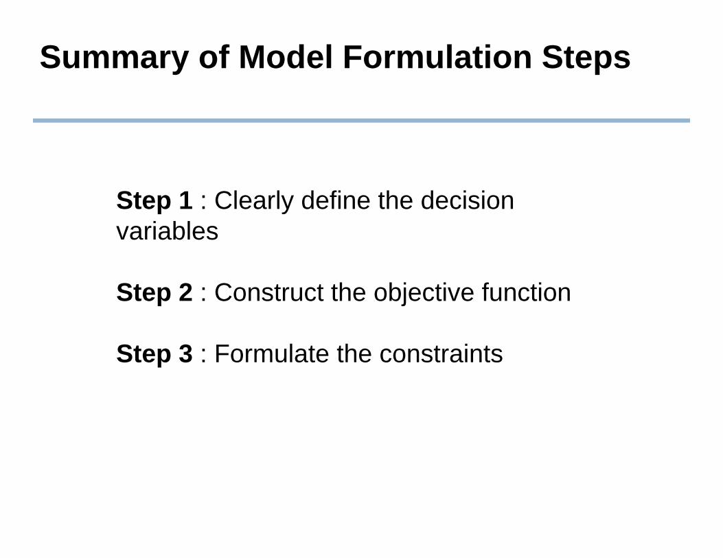
Step 1 : Clearly define the decision variables

Step 2 : Construct the objective function

Step 3 : Formulate the constraints

LP Model FormulationA Maximization Example (1 of 4)p ( )

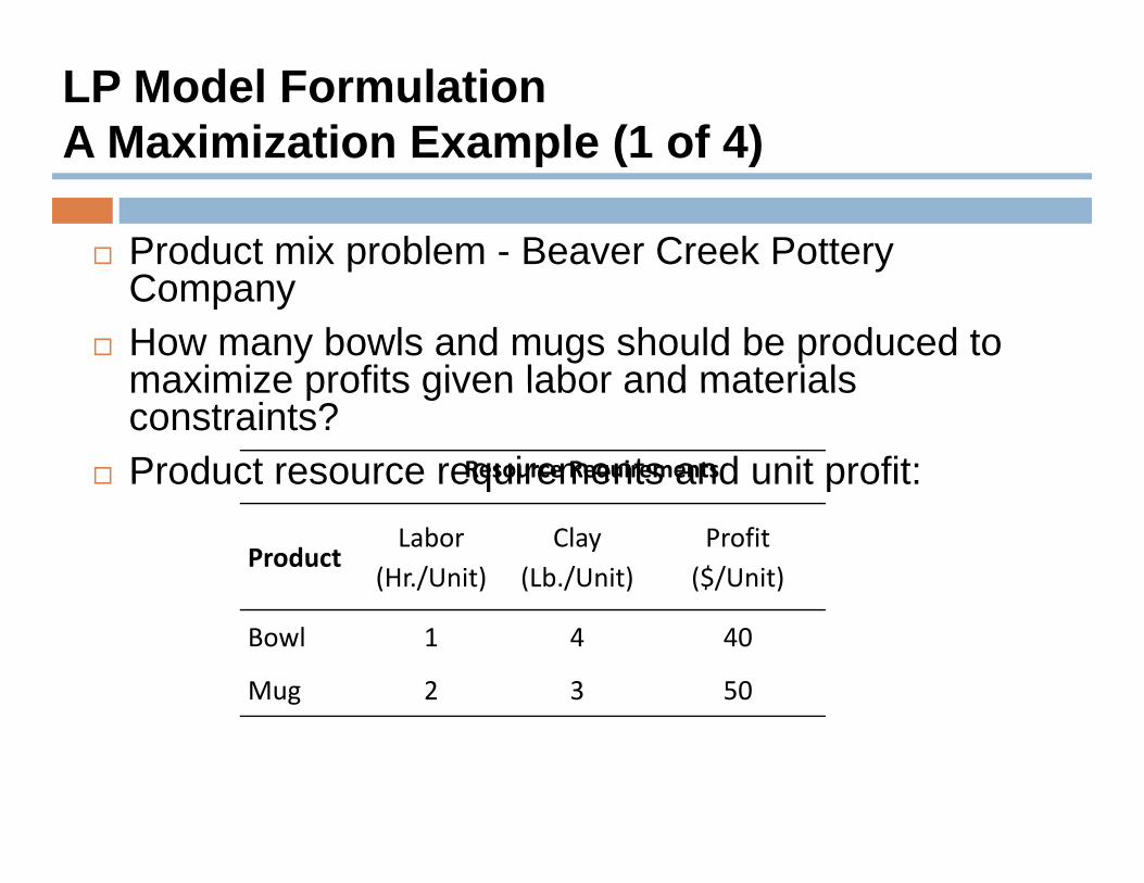
Product mix problem - Beaver Creek Pottery CCompanyHow many bowls and mugs should be produced to maximize profits given labor and materialsmaximize profits given labor and materials constraints?Product resource requirements and unit profit:Resource Requirements

ProductLabor

(Hr./Unit)Clay

(Lb./Unit)Profit($/Unit)

Bowl 1 4 40

Mug 2 3 50

LP Model FormulationA Maximization Example (2 of 4)p ( )

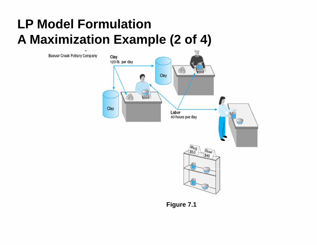
Figure 7.1

LP Model FormulationA Maximization Example (3 of 4)p ( )

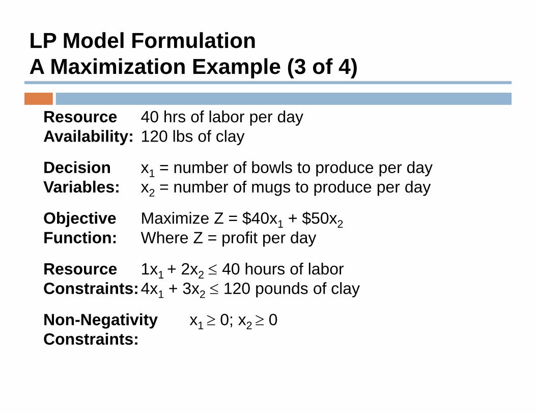
Resource 40 hrs of labor per dayAvailability: 120 lbs of clay

Decision x1 = number of bowls to produce per dayV i bl b f d dVariables: x2 = number of mugs to produce per day

Objective Maximize Z = $40x1 + $50x2F ti Wh Z fit dFunction: Where Z = profit per day

Resource 1x1 + 2x2 ≤ 40 hours of laborConstraints 4 + 3 ≤ 120 po nds of claConstraints:4x1 + 3x2 ≤ 120 pounds of clay

Non-Negativity x1 ≥ 0; x2 ≥ 0 Constraints:Constraints:

LP Model FormulationA Maximization Example (4 of 4)p ( )

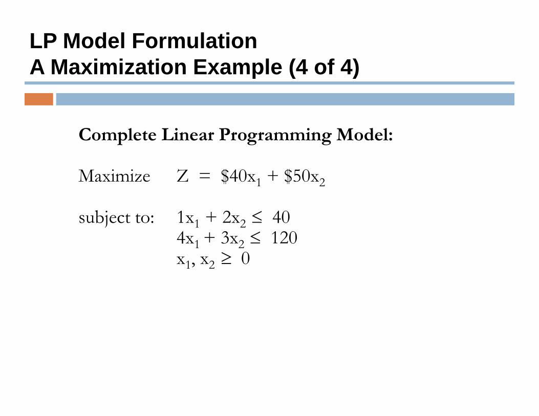
C l Li P i M d lComplete Linear Programming Model:

Maximize Z = $40x1 + $50x2$ 1 $ 2

subject to: 1x1 + 2x2 ≤ 404 + 3 ≤ 1204x1 + 3x2 ≤ 120x1, x2 ≥ 0

Feasible Solutions

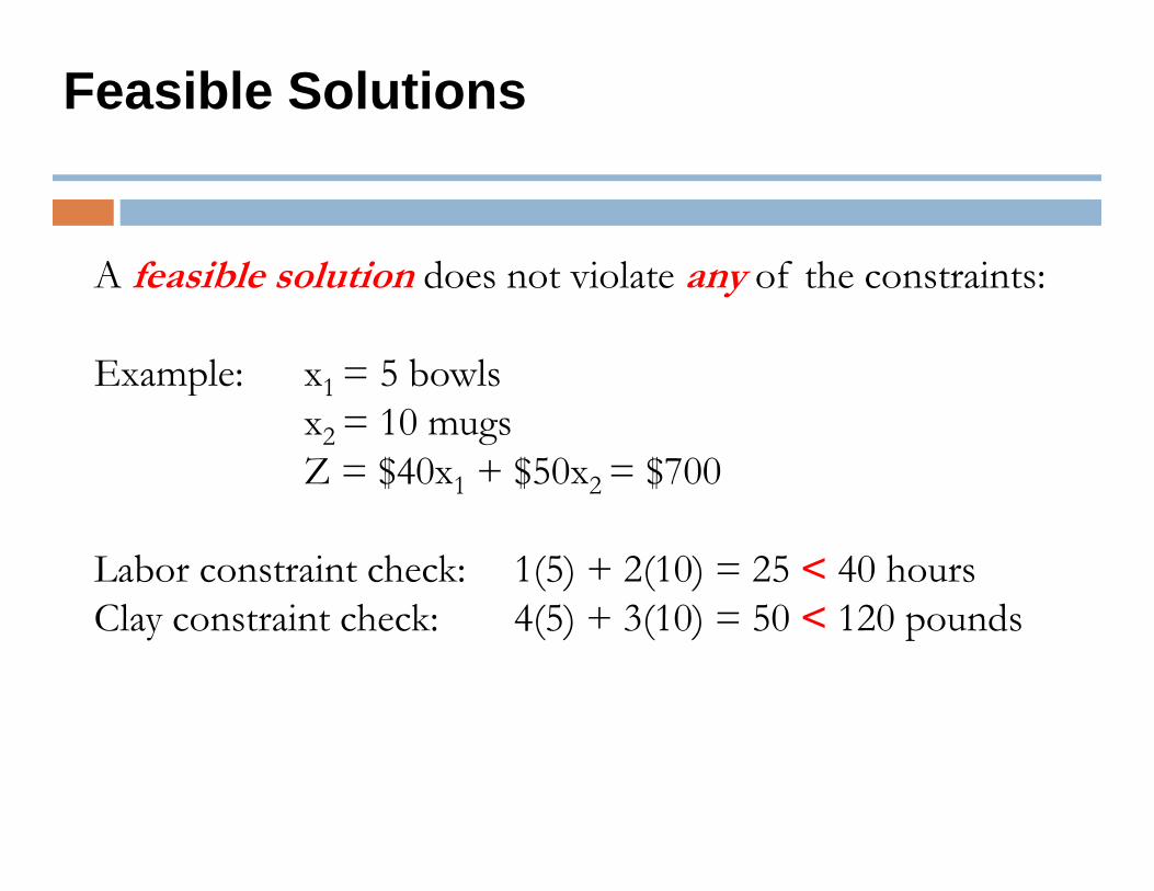
A feasible solution does not violate any of the constraints:A feasible solution does not violate any of the constraints:

Example: x1 = 5 bowlsp 1 x2 = 10 mugsZ = $40x1 + $50x2 = $700

Labor constraint check: 1(5) + 2(10) = 25 < 40 hours Cla constraint check 4(5) + 3(10) = 50 < 120 po ndsClay constraint check: 4(5) + 3(10) = 50 < 120 pounds

Infeasible Solutions

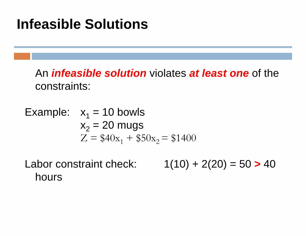
An infeasible solution violates at least one of theAn infeasible solution violates at least one of the constraints:

Example: x1 = 10 bowlsx2 = 20 mugsZ = $40x1 + $50x2 = $1400

Labor constraint check: 1(10) + 2(20) = 50 > 40Labor constraint check: 1(10) + 2(20) = 50 > 40 hours

Graphical Solution of LP Models

Graphical solution is limited to linear programming models containing only two p g g g ydecision variables (can be used with three variables but only with great difficulty).

Graphical methods provide visualization ofGraphical methods provide visualization of how a solution for a linear programming problem is obtained.p

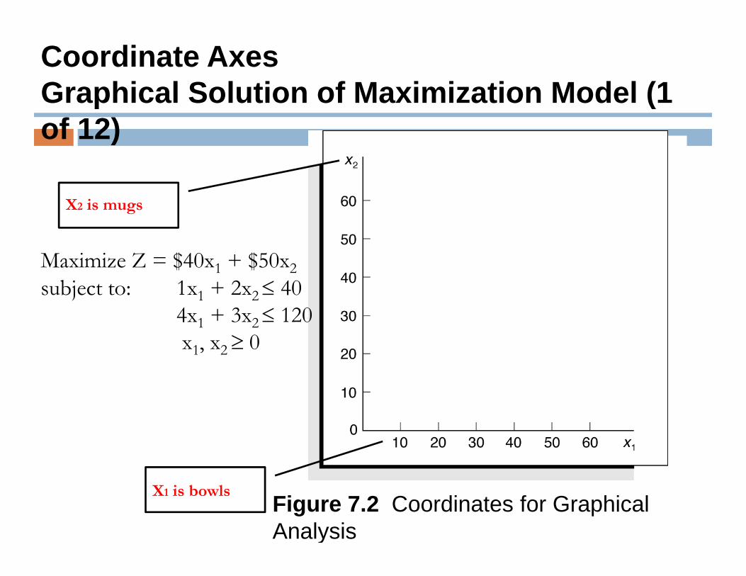
Coordinate AxesGraphical Solution of Maximization Model (1 p (of 12)

X2 is mugs

Maximize Z = $40x1 + $50x2subject to: 1x1 + 2x2 ≤ 40

4x1 + 3x2≤ 1201 2 x1, x2 ≥ 0

Figure 7.2 Coordinates for Graphical Analysis

X1 is bowls

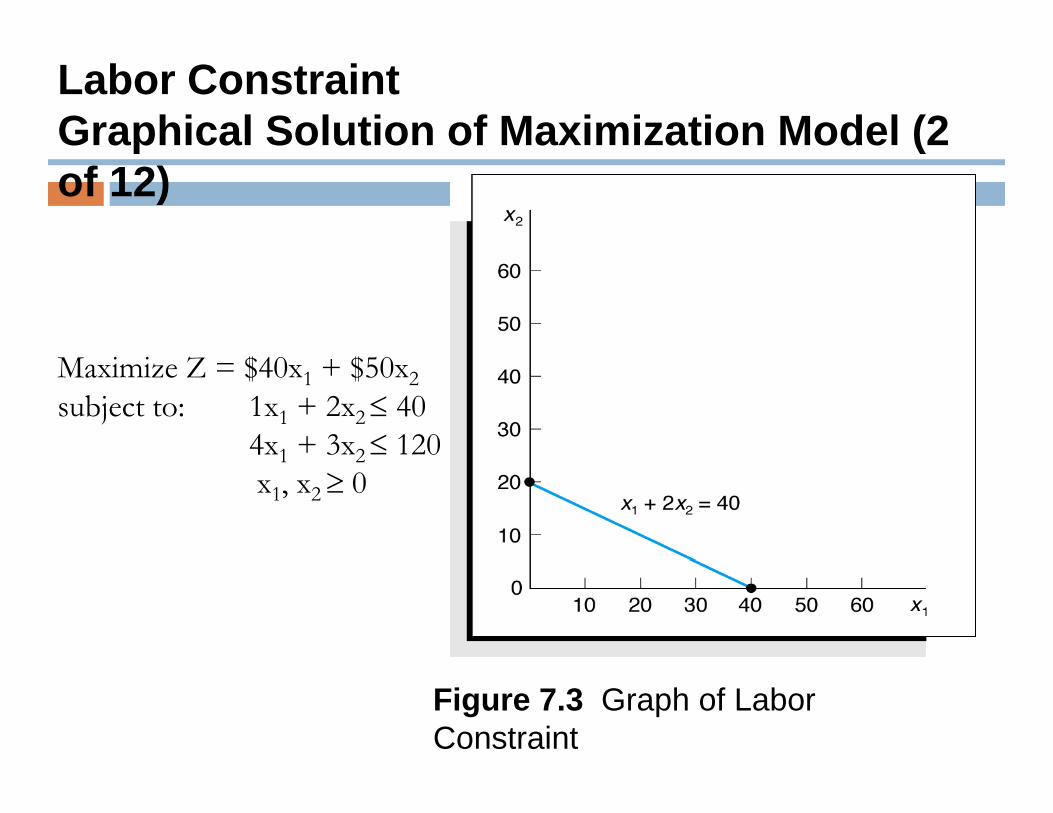
Labor ConstraintGraphical Solution of Maximization Model (2 p (of 12)

Maximize Z = $40x1 + $50x2subject to: 1x1 + 2x2 ≤ 40

4x1 + 3x2≤ 1201 2 x1, x2 ≥ 0

Figure 7.3 Graph of Labor Constraint

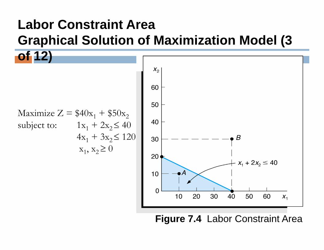
Labor Constraint AreaGraphical Solution of Maximization Model (3 p (of 12)

Maximize Z = $40x1 + $50x2subject to: 1x1 + 2x2 ≤ 40

4x1 + 3x2≤ 1201 2 x1, x2 ≥ 0

Figure 7.4 Labor Constraint Area

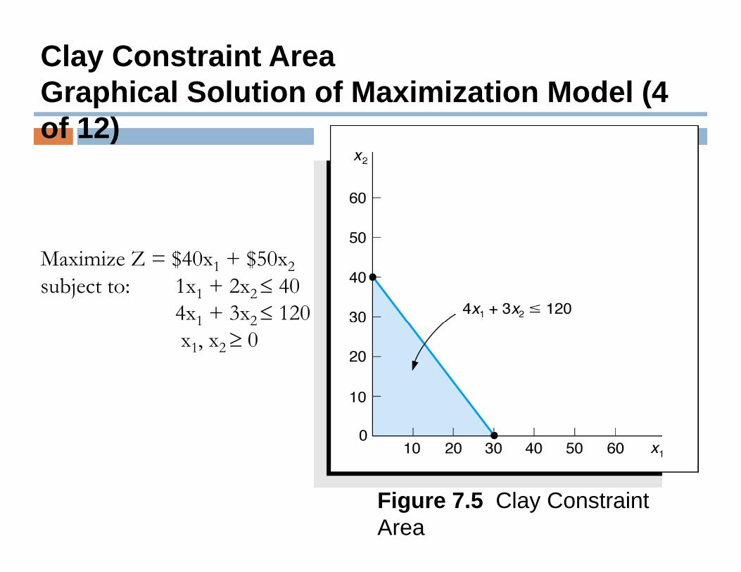
Clay Constraint AreaGraphical Solution of Maximization Model (4 p (of 12)

Maximize Z = $40x1 + $50x2subject to: 1x1 + 2x2 ≤ 40

4x1 + 3x2≤ 1201 2 x1, x2 ≥ 0

Figure 7.5 Clay Constraint Area

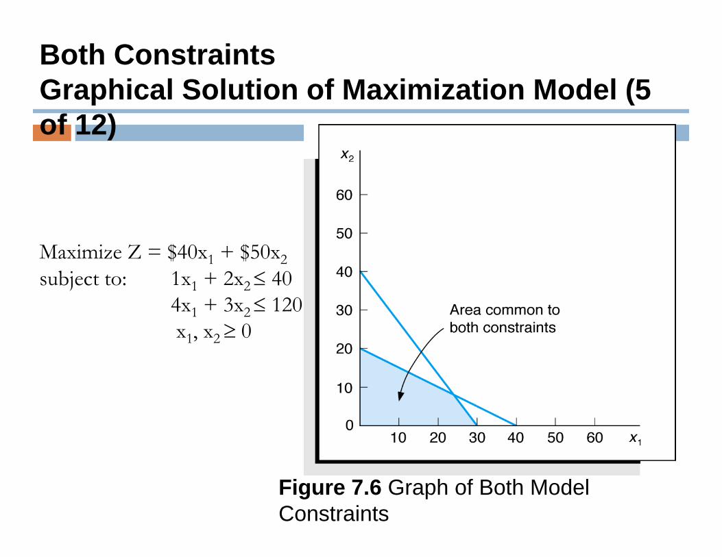
Both ConstraintsGraphical Solution of Maximization Model (5 p (of 12)

Maximize Z = $40x1 + $50x2subject to: 1x1 + 2x2 ≤ 40

4x1 + 3x2≤ 1201 2 x1, x2 ≥ 0

Figure 7.6 Graph of Both Model Constraints

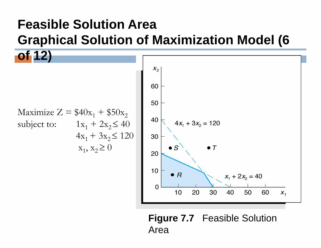
Feasible Solution AreaGraphical Solution of Maximization Model (6 p (of 12)

Maximize Z = $40x1 + $50x2subject to: 1x1 + 2x2 ≤ 40

4x1 + 3x2 ≤ 1201 2 x1, x2 ≥ 0

Figure 7.7 Feasible Solution Area

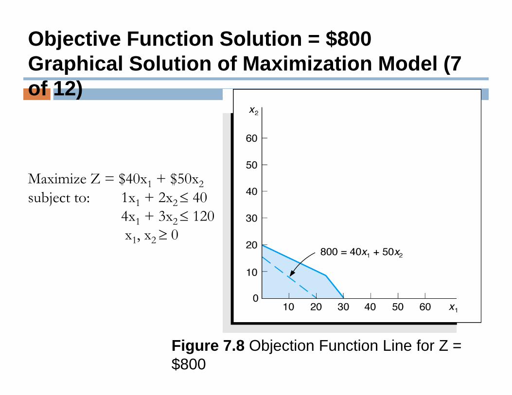
Objective Function Solution = $800Graphical Solution of Maximization Model (7 p (of 12)

Maximize Z = $40x1 + $50x2subject to: 1x1 + 2x2 ≤ 40

4x1 + 3x2≤ 1201 2 x1, x2 ≥ 0

Figure 7.8 Objection Function Line for Z = $800

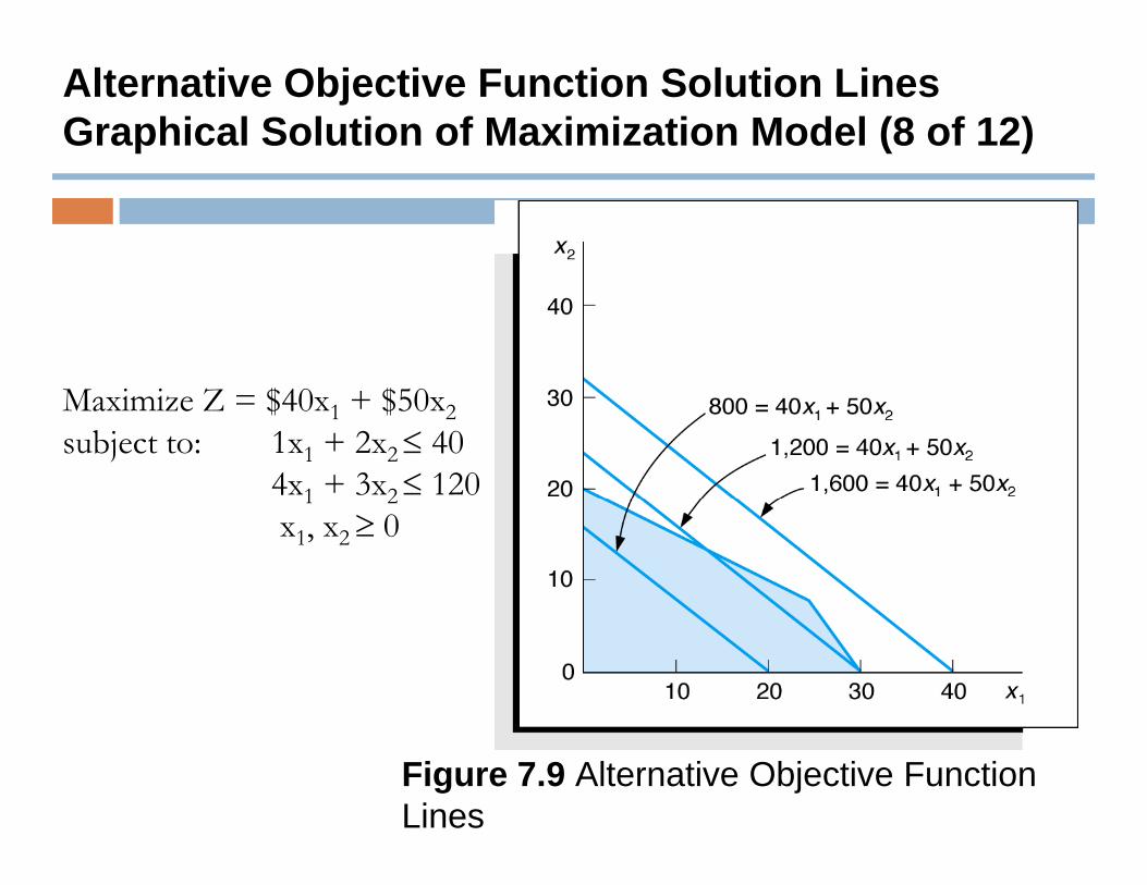
Alternative Objective Function Solution LinesGraphical Solution of Maximization Model (8 of 12)

Maximize Z = $40x1 + $50x2subject to: 1x1 + 2x2 ≤ 40

4x1 + 3x2≤ 1201 2 x1, x2 ≥ 0

Figure 7.9 Alternative Objective Function Lines

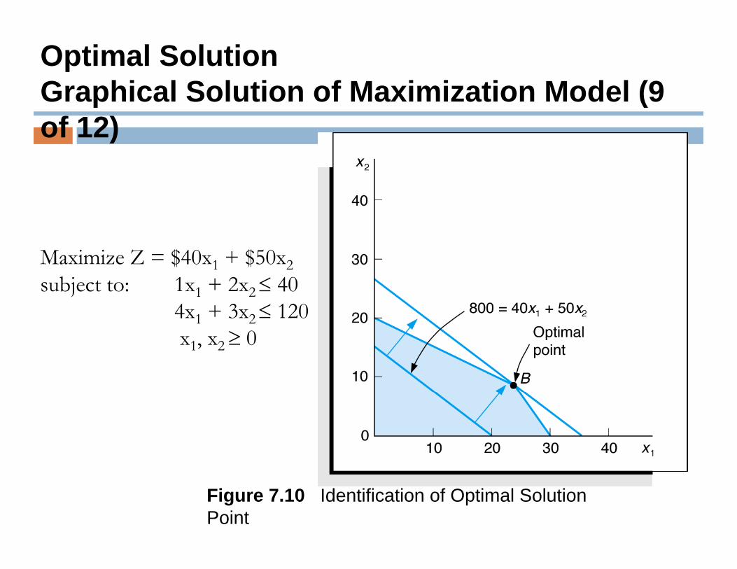
Optimal SolutionGraphical Solution of Maximization Model (9 p (of 12)

Maximize Z = $40x1 + $50x2subject to: 1x1 + 2x2 ≤ 40

4x1 + 3x2≤ 1201 2 x1, x2 ≥ 0

Figure 7.10 Identification of Optimal Solution Point

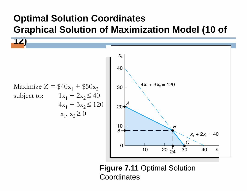
Optimal Solution CoordinatesGraphical Solution of Maximization Model (10 of 12)

Maximize Z = $40x1 + $50x2subject to: 1x1 + 2x2 ≤ 40

4x1 + 3x2≤ 1201 2 x1, x2 ≥ 0

Figure 7.11 Optimal Solution Coordinates

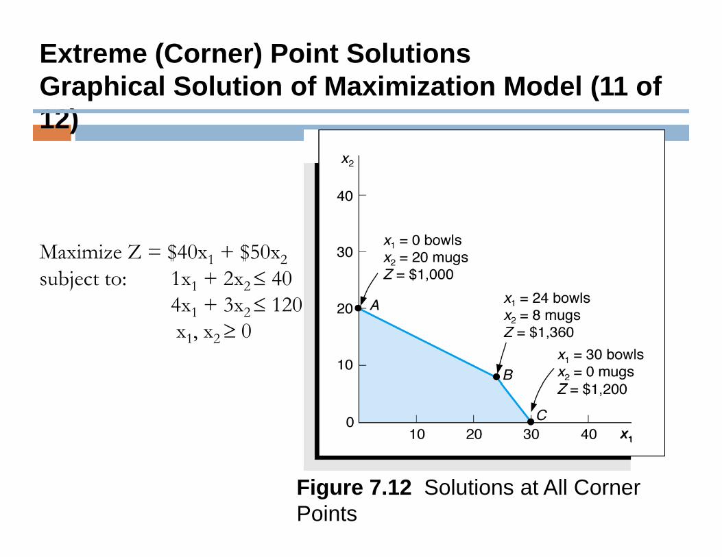
Extreme (Corner) Point SolutionsGraphical Solution of Maximization Model (11 of 12)

Maximize Z = $40x1 + $50x2subject to: 1x1 + 2x2 ≤ 40

4x1 + 3x2≤ 1201 2 x1, x2 ≥ 0

Figure 7.12 Solutions at All Corner Points

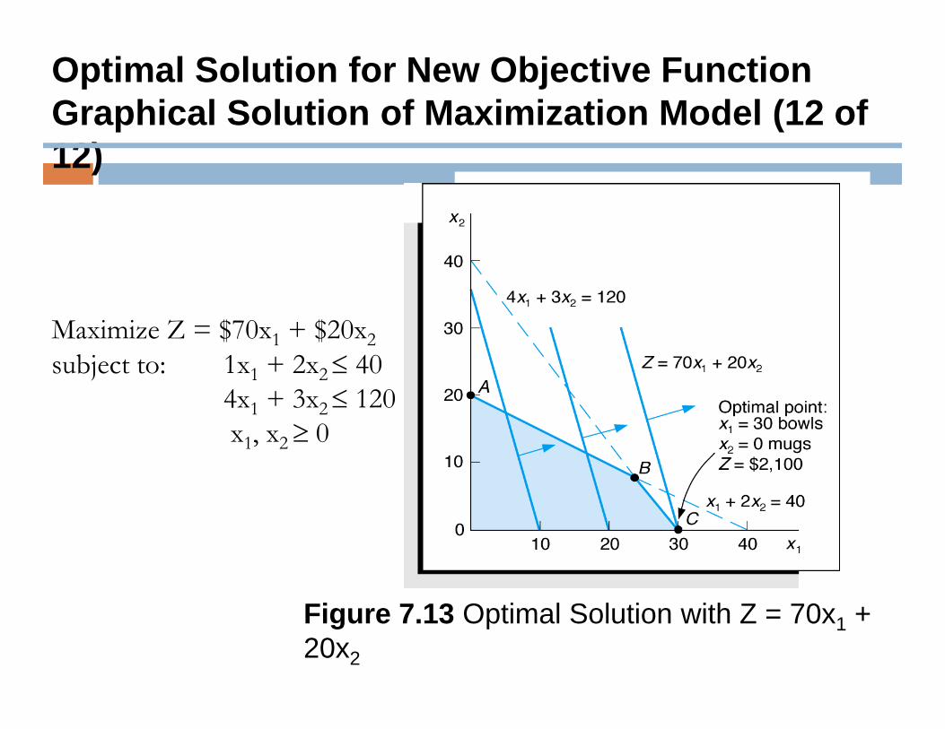
Optimal Solution for New Objective FunctionGraphical Solution of Maximization Model (12 of 12)

Maximize Z = $70x1 + $20x2subject to: 1x1 + 2x2 ≤ 40

4x1 + 3x2≤ 1201 2 x1, x2 ≥ 0

Figure 7.13 Optimal Solution with Z = 70x1 + 20x2

Slack Variables

Standard form requires that all constraints be inStandard form requires that all constraints be in the form of equations (equalities).A slack variable is added to a ≤ constraint (weakA slack variable is added to a ≤ constraint (weak inequality) to convert it to an equation (=).A slack variable typically represents an unusedA slack variable typically represents an unused resource.A slack variable contributes nothing to theA slack variable contributes nothing to the objective function value.

Linear Programming Model: Standard FormForm

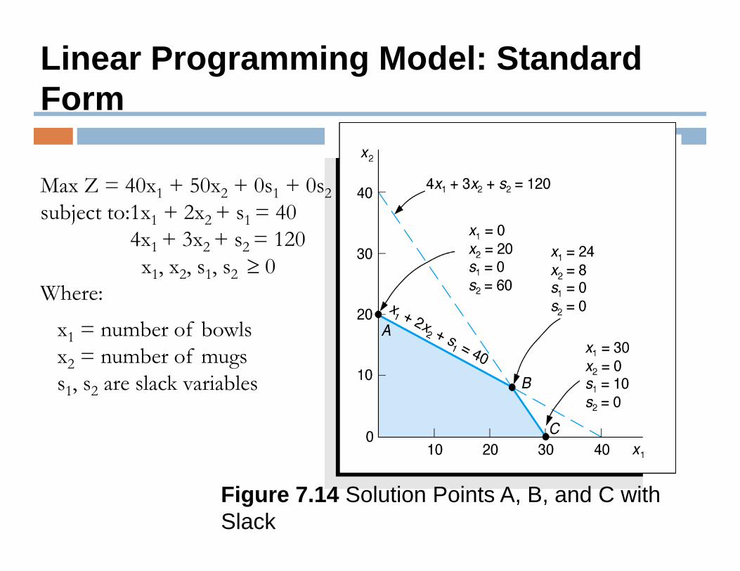
ZMax Z = 40x1 + 50x2 + 0s1 + 0s2subject to:1x1 + 2x2 + s1 = 40

4x1 + 3x2 + s2 = 1201 2 2 x1, x2, s1, s2 ≥ 0

Where:

b f b lx1 = number of bowlsx2 = number of mugss1, s2 are slack variables1, 2

Figure 7.14 Solution Points A, B, and C with Slack

LP Model Formulation – Minimization (1 of 8)

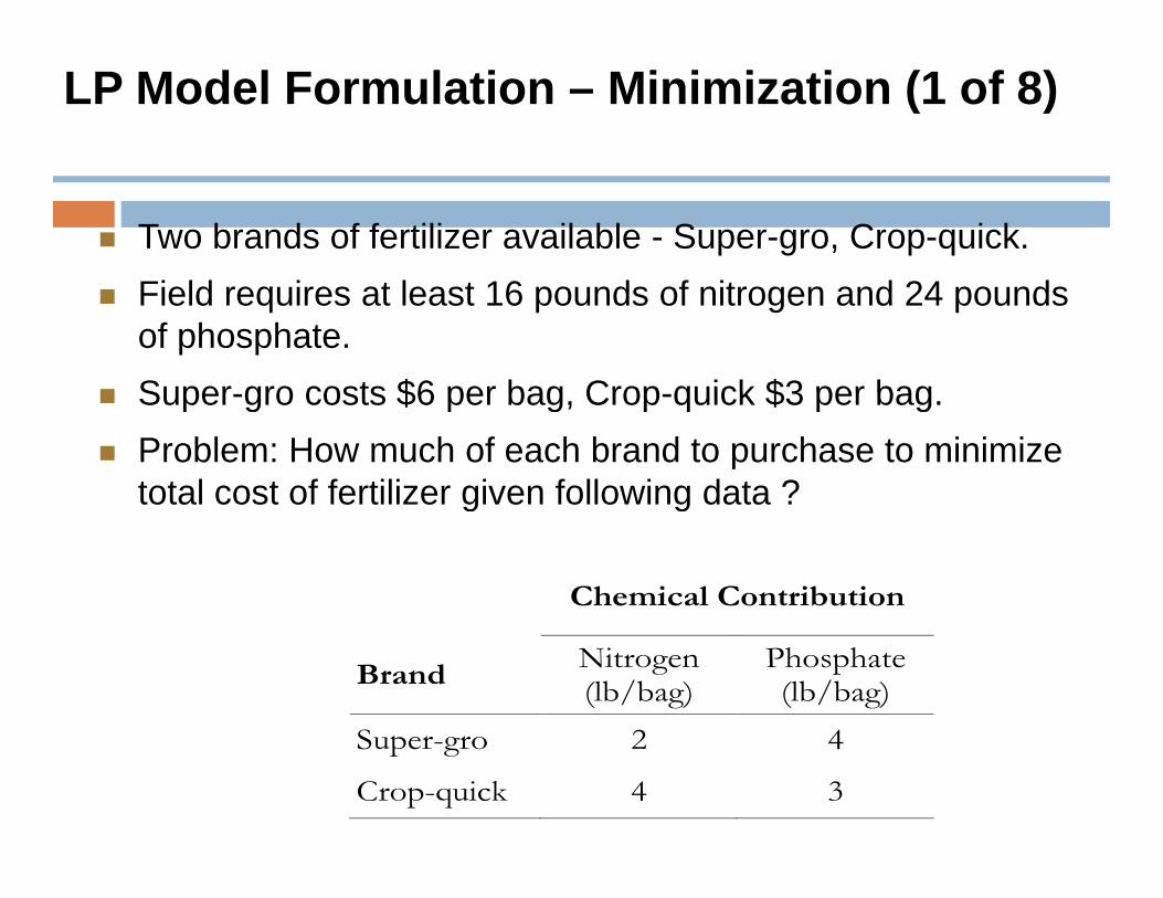
Two brands of fertilizer available - Super-gro, Crop-quick.Field requires at least 16 pounds of nitrogen and 24 pounds of phosphate.Super gro costs $6 per bag Crop quick $3 per bagSuper-gro costs $6 per bag, Crop-quick $3 per bag.Problem: How much of each brand to purchase to minimize total cost of fertilizer given following data ?

Chemical Contribution

g g

Brand Nitrogen (lb/bag)

Phosphate (lb/bag)

S 2 4Super-gro 2 4

Crop-quick 4 3

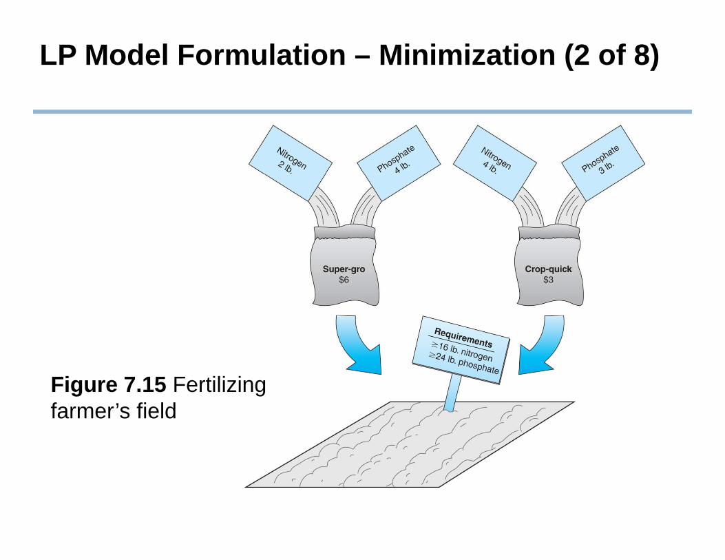
LP Model Formulation – Minimization (2 of 8)

Figure 7 15 FertilizingFigure 7.15 Fertilizing farmer’s field

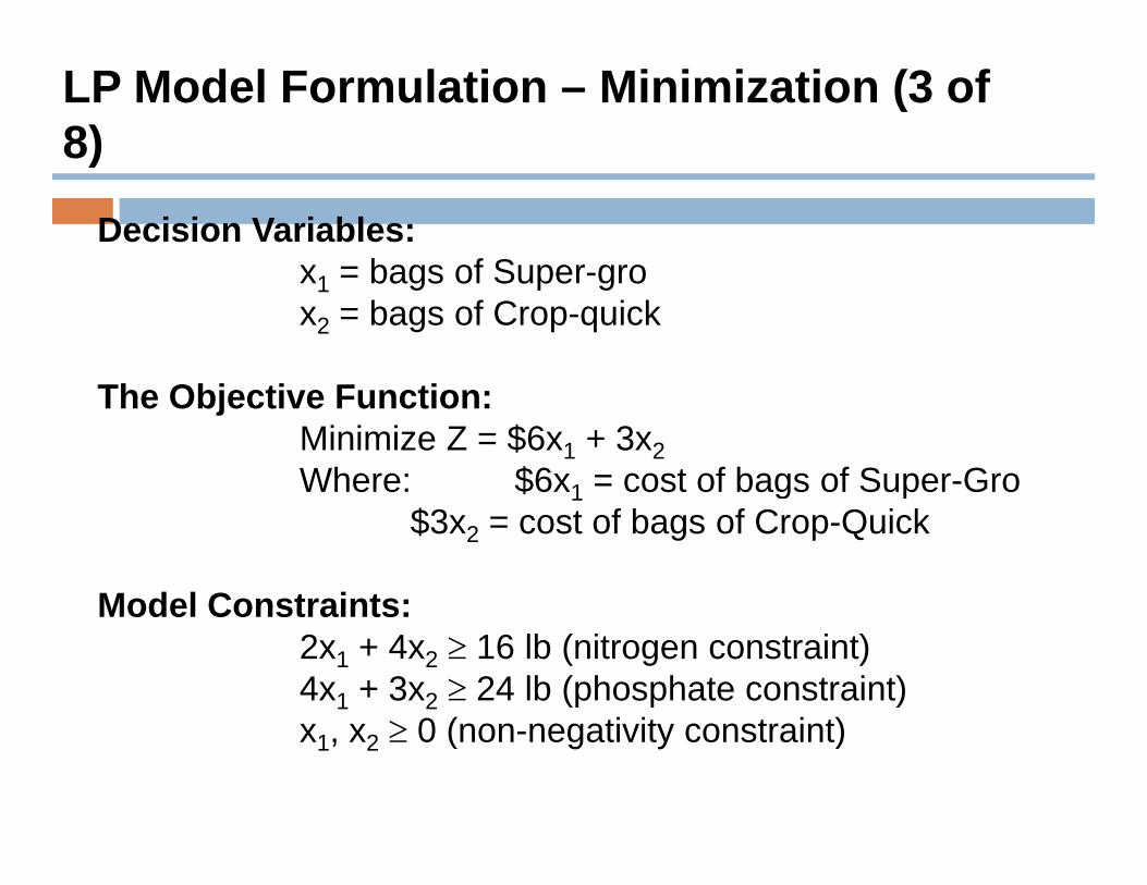
LP Model Formulation – Minimization (3 of 8)

Decision Variables:x1 = bags of Super-gro

)

x1 = bags of Super-grox2 = bags of Crop-quick

Th Obj ti F tiThe Objective Function:Minimize Z = $6x1 + 3x2Where: $6x1 = cost of bags of Super-Gro1 g p

$3x2 = cost of bags of Crop-Quick

Model Constraints:Model Constraints:2x1 + 4x2 ≥ 16 lb (nitrogen constraint)4x1 + 3x2 ≥ 24 lb (phosphate constraint)

≥ 0 ( ti it t i t)x1, x2 ≥ 0 (non-negativity constraint)

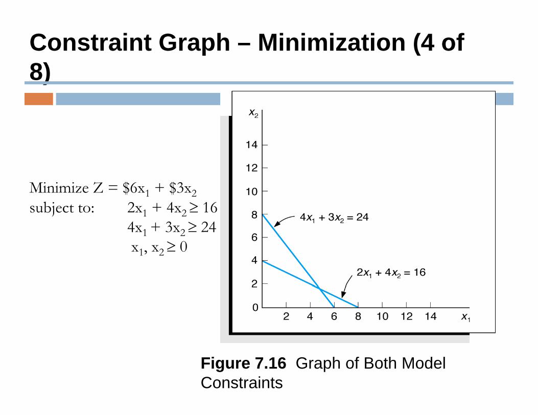
Constraint Graph – Minimization (4 of 8)8)

Minimize Z = $6x1 + $3x2subject to: 2x1 + 4x2 ≥ 16

4x1 + 3x2 ≥ 241 2 x1, x2 ≥ 0

Figure 7.16 Graph of Both Model Constraints

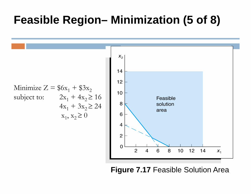
Feasible Region– Minimization (5 of 8)

Minimize Z = $6x1 + $3x2subject to: 2x1 + 4x2 ≥ 16

4x1 + 3x2≥ 241 2 x1, x2 ≥ 0

Figure 7.17 Feasible Solution Area

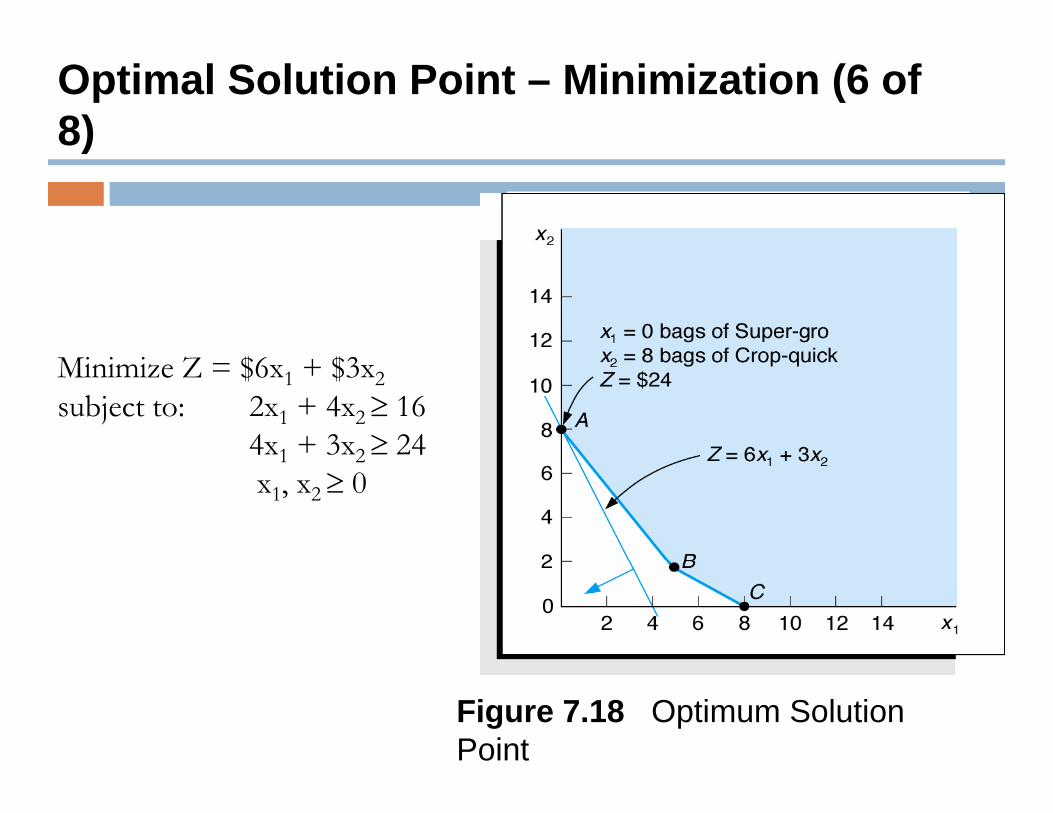
Optimal Solution Point – Minimization (6 of 8))

Minimize Z = $6x1 + $3x2subject to: 2x1 + 4x2 ≥ 16

4x1 + 3x2≥ 241 2 x1, x2 ≥ 0

Figure 7.18 Optimum Solution Point

Surplus Variables – Minimization (7 of 8)

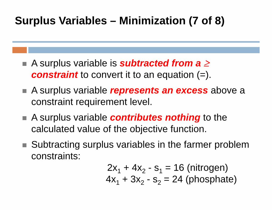
A surplus variable is subtracted from a ≥A surplus variable is subtracted from a ≥constraint to convert it to an equation (=).A surplus variable represents an excess above aA surplus variable represents an excess above a constraint requirement level.A surplus variable contributes nothing to theA surplus variable contributes nothing to the calculated value of the objective function.Subtracting surplus variables in the farmer problemSubtracting surplus variables in the farmer problem constraints:

2x1 + 4x2 - s1 = 16 (nitrogen)1 2 1 ( g )4x1 + 3x2 - s2 = 24 (phosphate)

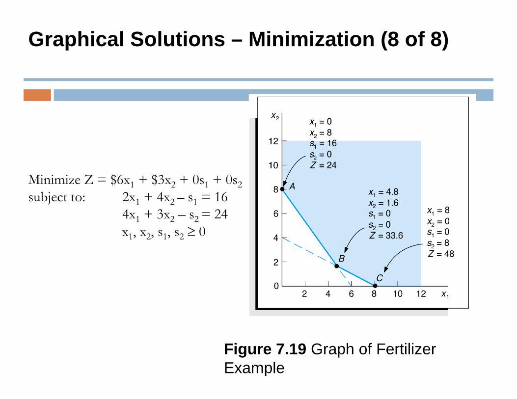
Graphical Solutions – Minimization (8 of 8)

Minimize Z = $6x1 + $3x2 + 0s1 + 0s2subject to: 2x1 + 4x2 – s1 = 16

4x1 + 3x2 – s2 = 24x1, x2, s1, s2 ≥ 0

Figure 7.19 Graph of Fertilizer Example

Irregular Types of Linear Programming Problems

For some linear programming models theFor some linear programming models, the general rules do not apply.

Special types of problems include those with:Multiple optimal solutionsInfeasible solutionsUnbounded solutions

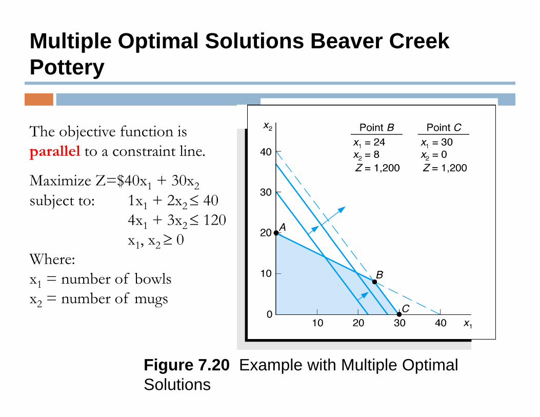
Multiple Optimal Solutions Beaver Creek Potteryy

The objecti e f nction isThe objective function is parallel to a constraint line.

Maximize Z=$40x + 30xMaximize Z=$40x1 + 30x2subject to: 1x1 + 2x2 ≤ 40

4x1 + 3x2 ≤ 120≥ 0x1, x2 ≥ 0

Where:x1 = number of bowls1x2 = number of mugs

Figure 7.20 Example with Multiple Optimal Solutions

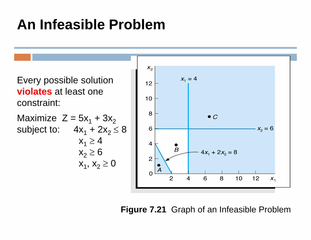
An Infeasible Problem

Every possible solution violates at least one constraint:constraint:Maximize Z = 5x1 + 3x2subject to: 4x1 + 2x2 ≤ 8

x1 ≥ 4x2 ≥ 6x1 x2 ≥ 0x1, x2 ≥ 0

Figure 7.21 Graph of an Infeasible Problem

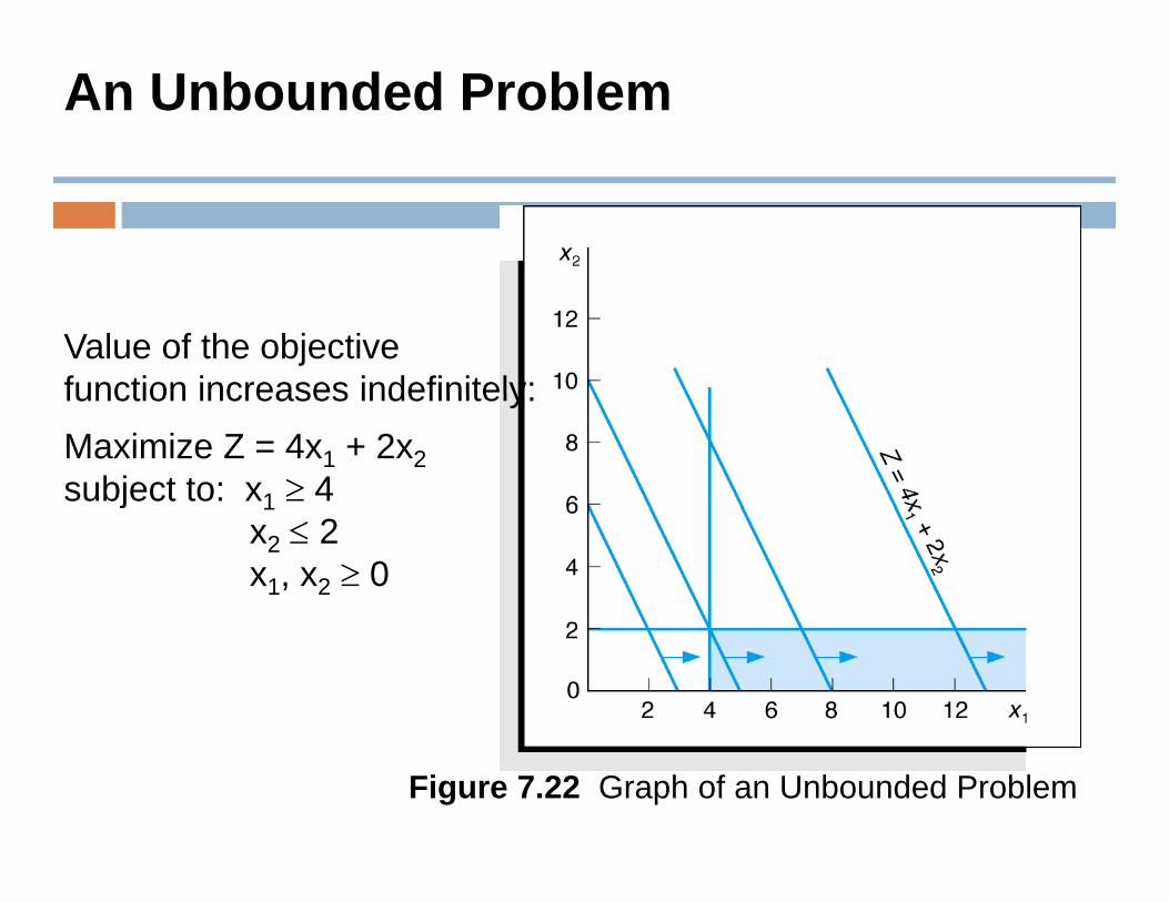
An Unbounded Problem

Value of the objectivefunction increases indefinitely:function increases indefinitely:Maximize Z = 4x1 + 2x2subject to: x1 ≥ 4j 1

x2 ≤ 2x1, x2 ≥ 0

Figure 7.22 Graph of an Unbounded Problem

Characteristics of Linear Programming Problems

A decision amongst alternative courses of action gis required.The decision is represented in the model by decision variablesdecision variables.The problem encompasses a goal, expressed as an objective function, that the decision maker

hiwants to achieve.Restrictions (represented by constraints) exist that limit the extent of achievement of thethat limit the extent of achievement of the objective.The objective and constraints must be definable b li th ti l f ti l l ti hiby linear mathematical functional relationships.

Properties of Linear Programming Models

Proportionality - The rate of change (slope) of

Models

Proportionality The rate of change (slope) of the objective function and constraint equations is constant.Additivity - Terms in the objective function and constraint equations must be additive.Divisibility -Decision variables can take on any fractional value and are therefore continuous as opposed to integer in nature.Certainty - Values of all the model parameters

d b k i h i (are assumed to be known with certainty (non-probabilistic).

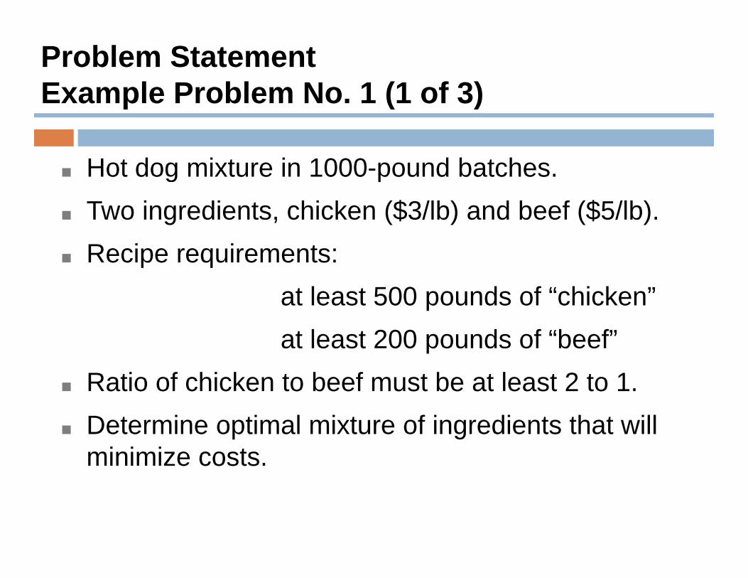
Problem StatementExample Problem No. 1 (1 of 3)p ( )

■ Hot dog mixture in 1000-pound batches.g p■ Two ingredients, chicken ($3/lb) and beef ($5/lb).

Recipe requirements:■ Recipe requirements:at least 500 pounds of “chicken”at least 200 pounds of “beef”

■ Ratio of chicken to beef must be at least 2 to 1.■ Determine optimal mixture of ingredients that will

minimize costs.

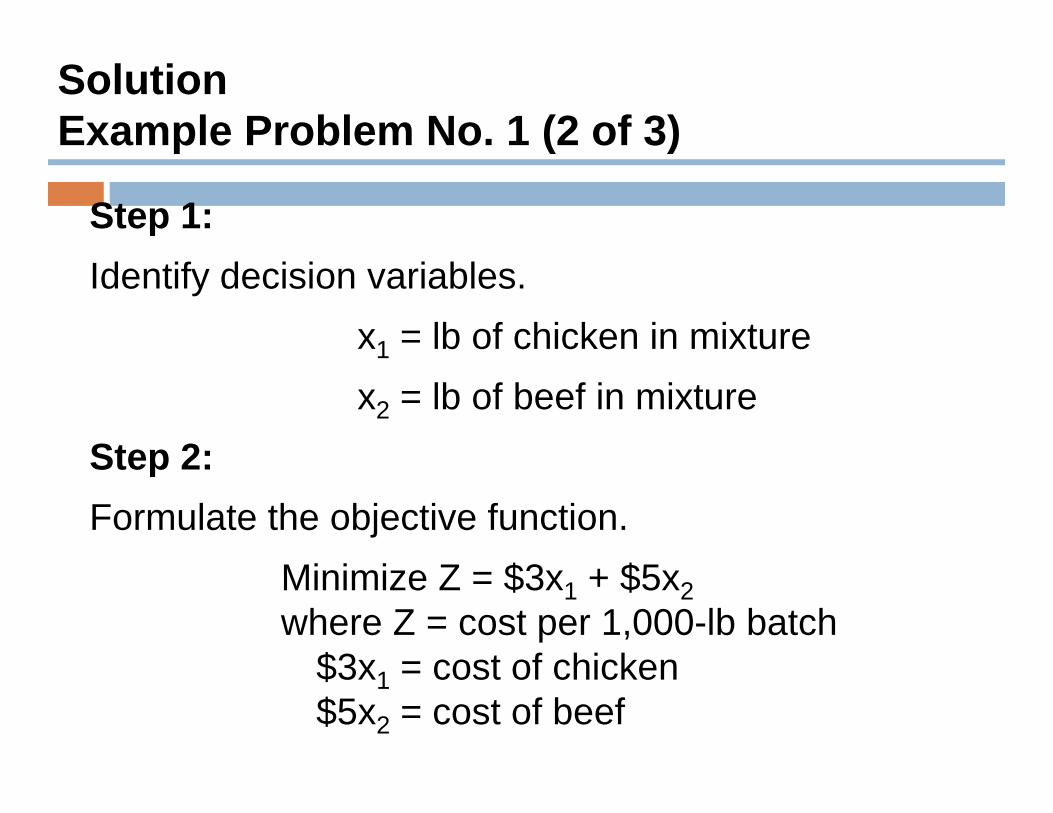
SolutionExample Problem No. 1 (2 of 3)

Step 1:

p ( )

Identify decision variables.x1 = lb of chicken in mixture1

x2 = lb of beef in mixtureStep 2:Step 2:Formulate the objective function.

Minimize Z = $3x1 + $5x2where Z = cost per 1,000-lb batch

$3x = cost of chicken$3x1 = cost of chicken$5x2 = cost of beef

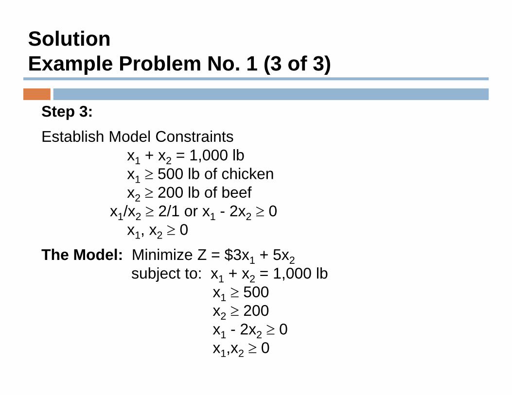
SolutionExample Problem No. 1 (3 of 3)

Step 3:

p ( )

Establish Model Constraintsx1 + x2 = 1,000 lbx ≥ 500 lb of chickenx1 ≥ 500 lb of chickenx2 ≥ 200 lb of beef

x1/x2 ≥ 2/1 or x1 - 2x2 ≥ 0x1, x2 ≥ 0

The Model: Minimize Z = $3x1 + 5x2subject to: x + x = 1 000 lbsubject to: x1 + x2 = 1,000 lb

x1 ≥ 500x2 ≥ 200 x1 - 2x2 ≥ 0x1,x2 ≥ 0

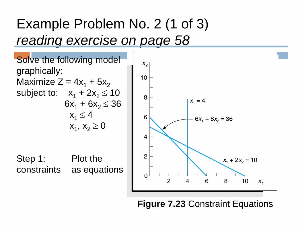
Example Problem No. 2 (1 of 3)reading exercise on page 58Solve the following model graphically:

reading exercise on page 58

graphically:Maximize Z = 4x1 + 5x2subject to: x1 + 2x2 ≤ 10

6 + 6 ≤ 366x1 + 6x2 ≤ 36x1 ≤ 4x1, x2 ≥ 0

Step 1: Plot theStep 1: Plot the constraints as equations

Figure 7.23 Constraint Equations

Example Problem No. 2 (2 of 3)

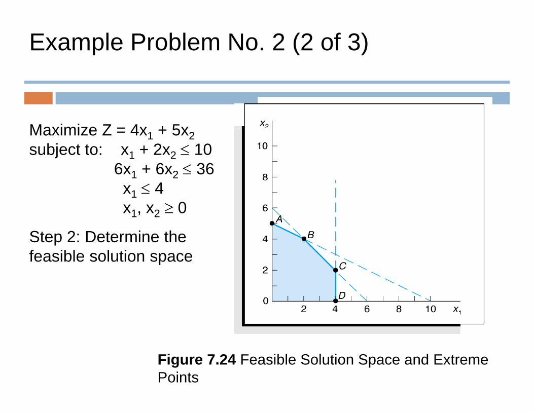
Maximize Z = 4x + 5xMaximize Z = 4x1 + 5x2subject to: x1 + 2x2 ≤ 10

6x1 + 6x2 ≤ 36x1 ≤ 4x1, x2 ≥ 0

St 2 D t i thStep 2: Determine the feasible solution space

Figure 7.24 Feasible Solution Space and Extreme Points

Example Problem No. 2 (3 of 3)

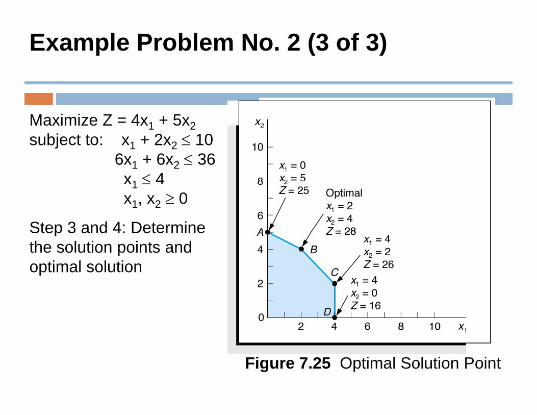
Maximize Z = 4x1 + 5x21 2subject to: x1 + 2x2 ≤ 10

6x1 + 6x2 ≤ 36x1 ≤ 4x1 ≤ 4x1, x2 ≥ 0

Step 3 and 4: Determine pthe solution points and optimal solution

Figure 7.25 Optimal Solution Point

Assignmentg

Q 1 An Aeroplane can carry a maximum of 200 passengers AQ.1 An Aeroplane can carry a maximum of 200 passengers. A profit of Rs. 400 is made on each first class ticket and a profit of Rs. 300 is made on each economy class ticket. The airline reserves at least 20 seats for first class. However, at least 4 timesreserves at least 20 seats for first class. However, at least 4 times as many passengers prefer to travel by economy class than by the first class. How many tickets of each class must be sold in order to maximize profit for the airline? Formulate the problem as an mode.

Q.2 Solve the LPP by Graphical method :

Minimize z = 20x+10y Minimize z = 20x+10y

Subject to the constraints

x + 2y ≤ 40 , 3x+ y ≥ 30 , 4x+3y ≥ 60

x , y ≥ 0

Thank You