Linear programming - GitHub Pages · The simplex method does exactly this. Starting from any extreme point, the method moves along the edges of the feasible region to form a sequence

Linear programming

CE 367R

Linear programming

OVERVIEW

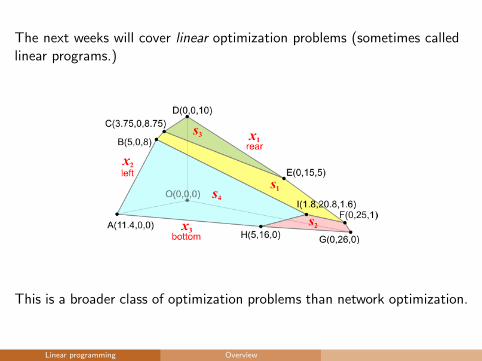
The next weeks will cover linear optimization problems (sometimes calledlinear programs.)

This is a broader class of optimization problems than network optimization.

Linear programming Overview

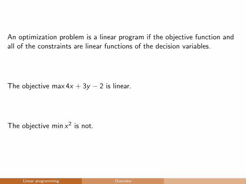
An optimization problem is a linear program if the objective function andall of the constraints are linear functions of the decision variables.

The objective max 4x + 3y − 2 is linear.

The objective min x2 is not.


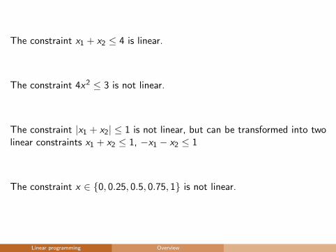
The constraint x1 + x2 ≤ 4 is linear.

The constraint 4x2 ≤ 3 is not linear.

The constraint |x1 + x2| ≤ 1 is not linear, but can be transformed into twolinear constraints x1 + x2 ≤ 1, −x1 − x2 ≤ 1

The constraint x ∈ {0, 0.25, 0.5, 0.75, 1} is not linear.


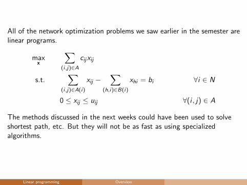
All of the network optimization problems we saw earlier in the semester arelinear programs.

maxx

∑(i ,j)∈A

cijxij

s.t.∑

(i ,j)∈A(i)

xij −∑

(h,i)∈B(i)

xhi = bi ∀i ∈ N

0 ≤ xij ≤ uij ∀(i , j) ∈ A

The methods discussed in the next weeks could have been used to solveshortest path, etc. But they will not be as fast as using specializedalgorithms.


EXAMPLES

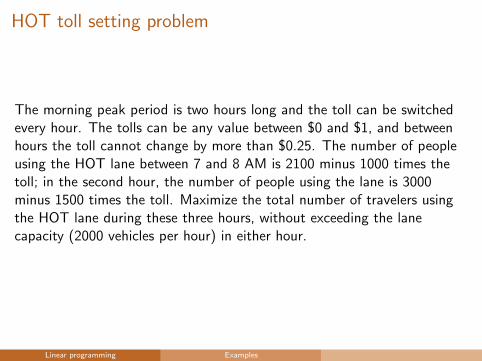
HOT toll setting problem

The morning peak period is two hours long and the toll can be switchedevery hour. The tolls can be any value between $0 and $1, and betweenhours the toll cannot change by more than $0.25. The number of peopleusing the HOT lane between 7 and 8 AM is 2100 minus 1000 times thetoll; in the second hour, the number of people using the lane is 3000minus 1500 times the toll. Maximize the total number of travelers usingthe HOT lane during these three hours, without exceeding the lanecapacity (2000 vehicles per hour) in either hour.

Linear programming Examples

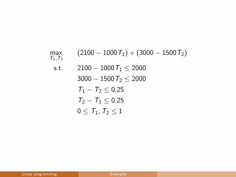
maxT1,T2

(2100− 1000T1) + (3000− 1500T2)

s.t. 2100− 1000T1 ≤ 2000

3000− 1500T2 ≤ 2000

T1 − T2 ≤ 0.25

T2 − T1 ≤ 0.25

0 ≤ T1,T2 ≤ 1


A production problem

A firm produces n different goods using m raw materials.

For each raw material i , bi units are available.

Producing a unit of the j-th good requires aij units of material i , andresults in a profit of cj .

What should we do to maximize profit?


Production planning by a computer manufacturer

See example on Canvas for a more involved version of the productionproblem, with different types of computer systems, constraints based ondemand for different types of systems, and so forth.


A scheduling problem

A hospital wants to make a weekly night shift schedule for its nurses; onday j a total of dj nurses are needed (j ∈ {1, 2, . . . , 7}).

Every nurse works five days in a row. What is the minimum number ofnurses that are needed to cover the shifts?


GEOMETRY

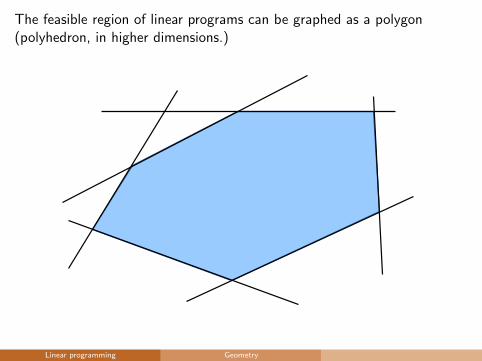
The feasible region of linear programs can be graphed as a polygon(polyhedron, in higher dimensions.)

Linear programming Geometry

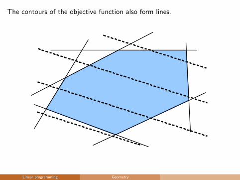
The contours of the objective function also form lines.


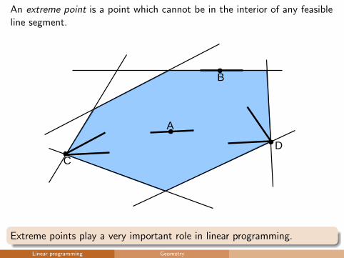
An extreme point is a point which cannot be in the interior of any feasibleline segment.

A

B

C

D

Extreme points play a very important role in linear programming.


The following result is very important:

If a linear program has a global optimal solution and the feasible region hasan extreme point, at least one of the extreme points is globally optimal.

In other words, for linear programs, we only need to look at extreme points.




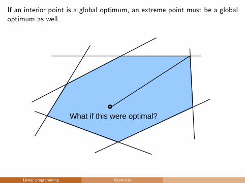
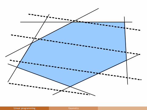
If an interior point is a global optimum, an extreme point must be a globaloptimum as well.

What if this were optimal?


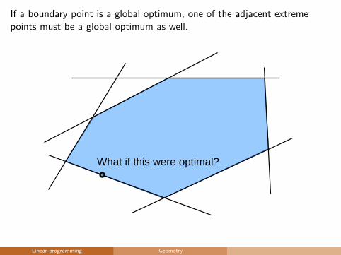
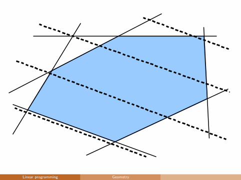
If a boundary point is a global optimum, one of the adjacent extremepoints must be a global optimum as well.

What if this were optimal?


A NAIVE SOLUTIONMETHOD

Since at least one of the extreme points is optimal, and there is a finitenumber of extreme points, we can find them all and check them one byone.

Linear programming A naıve solution method

This method works, but has a few drawbacks:

If there are more than two decision variables, it is hard to draw thefeasible region and spot the extreme points?

The number of extreme points is O(2m) (where m is the number ofconstraints), so checking them all in large problems is impossible.


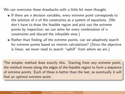
We can overcome these drawbacks with a little bit more thought.

If there are n decision variables, every extreme point corresponds tothe solution of n of the constraints as a system of equations. (Wedon’t have to draw the feasible region and pick out the extremepoints by inspection; we can solve for every combination of nconstraints and discard the infeasible ones.)

Rather than finding all the extreme points, can we adaptively searchfor extreme points based on interim calculations? (Since the objectiveis linear, we never need to search “uphill” from where we are.)

The simplex method does exactly this. Starting from any extreme point,the method moves along the edges of the feasible region to form a sequenceof extreme points. Each of these is better than the last, so eventually it willfind an optimal extreme point.


STANDARD FORM

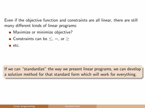
Even if the objective function and constraints are all linear, there are stillmany different kinds of linear programs:

Maximize or minimize objective?

Constraints can be ≤, =, or ≥etc.

If we can “standardize” the way we present linear programs, we can developa solution method for that standard form which will work for everything.

Linear programming Standard form

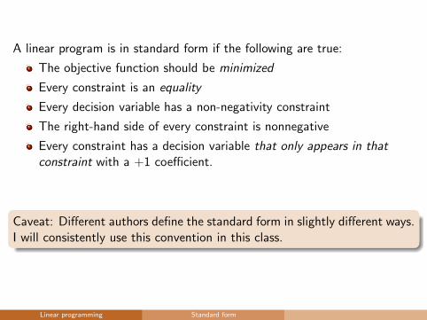
A linear program is in standard form if the following are true:

The objective function should be minimized

Every constraint is an equality

Every decision variable has a non-negativity constraint

The right-hand side of every constraint is nonnegative

Every constraint has a decision variable that only appears in thatconstraint with a +1 coefficient.

Caveat: Different authors define the standard form in slightly different ways.I will consistently use this convention in this class.


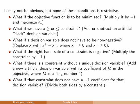
It may not be obvious, but none of these conditions is restrictive.

What if the objective function is to be minimized? (Multiply it by −1and maximize it.)

What if we have a ≥ or ≤ constraint? (Add or subtract an artificial“slack” decision variable.)

What if a decision variable does not have to be non-negative?(Replace x with x+ − x−, where x+ ≥ 0 and x− ≥ 0).

What if the right-hand side of a constraint is negative? (Multiply theconstraint by −1.)

What if there is a constraint without a unique decision variable? (Adda new artificial decision variable, with a coefficient of M in theobjective, where M is a “big number.”)

What if that constraint does not have a +1 coefficient for thatdecision variable? (Divide both sides by a constant.)


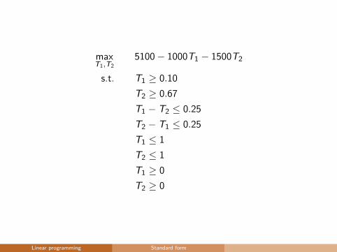
maxT1,T2

5100− 1000T1 − 1500T2

s.t. T1 ≥ 0.10

T2 ≥ 0.67

T1 − T2 ≤ 0.25

T2 − T1 ≤ 0.25

T1 ≤ 1

T2 ≤ 1

T1 ≥ 0

T2 ≥ 0


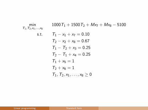
minT1,T2,x1,...,x8

1000T1 + 1500T2 + Mx7 + Mx8 − 5100

s.t. T1 − x1 + x7 = 0.10

T2 − x2 + x8 = 0.67

T1 − T2 + x3 = 0.25

T2 − T1 + x4 = 0.25

T1 + x5 = 1

T2 + x6 = 1

T1,T2, x1, . . . , x8 ≥ 0


SIMPLEX METHOD

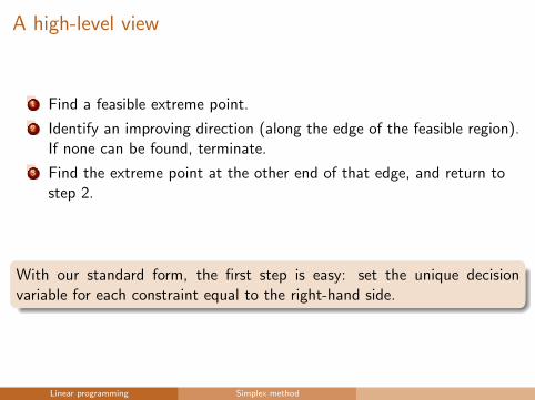
A high-level view

1 Find a feasible extreme point.

2 Identify an improving direction (along the edge of the feasible region).If none can be found, terminate.

3 Find the extreme point at the other end of that edge, and return tostep 2.

With our standard form, the first step is easy: set the unique decisionvariable for each constraint equal to the right-hand side.

Linear programming Simplex method

Motivating Example

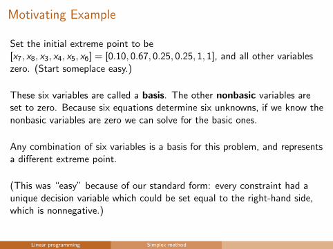
Set the initial extreme point to be[x7, x8, x3, x4, x5, x6] = [0.10, 0.67, 0.25, 0.25, 1, 1], and all other variableszero. (Start someplace easy.)

These six variables are called a basis. The other nonbasic variables areset to zero. Because six equations determine six unknowns, if we know thenonbasic variables are zero we can solve for the basic ones.

Any combination of six variables is a basis for this problem, and representsa different extreme point.

(This was “easy” because of our standard form: every constraint had aunique decision variable which could be set equal to the right-hand side,which is nonnegative.)


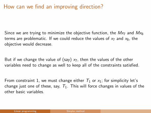
How can we find an improving direction?

Since we are trying to minimize the objective function, the Mx7 and Mx8

terms are problematic. If we could reduce the values of x7 and x8, theobjective would decrease.

But if we change the value of (say) x7, then the values of the othervariables need to change as well to keep all of the constraints satisfied.

From constraint 1, we must change either T1 or x1; for simplicity let’schange just one of these, say, T1. This will force changes in values of theother basic variables.


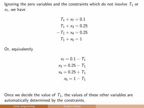
Ignoring the zero variables and the constraints which do not inovlve T1 orx7, we have

T1 + x7 = 0.1

T1 + x3 = 0.25

−T1 + x4 = 0.25

T1 + x5 = 1

Or, equivalently

x7 = 0.1− T1

x3 = 0.25− T1

x4 = 0.25 + T1

x5 = 1− T1

Once we decide the value of T1, the values of these other variables areautomatically determined by the constraints.


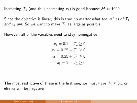
Increasing T1 (and thus decreasing x7) is good because M � 1000.

Since the objective is linear, this is true no matter what the values of T1

and x7 are. So we want to make T1 as large as possible.

However, all of the variables need to stay nonnegative

x7 = 0.1− T1 ≥ 0

x3 = 0.25− T1 ≥ 0

x4 = 0.25 + T1 ≥ 0

x5 = 1− T1 ≥ 0

The most restrictive of these is the first one, we must have T1 ≤ 0.1 orelse x7 will be negative.


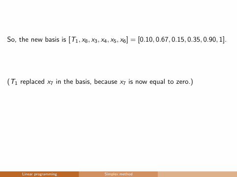
So, the new basis is [T1, x8, x3, x4, x5, x6] = [0.10, 0.67, 0.15, 0.35, 0.90, 1].

(T1 replaced x7 in the basis, because x7 is now equal to zero.)


This process can become more complicated after the initial iterations: aswe change one decision variable, many others may have to change (notjust one variable per equation) and the effects of the objective function areharder to spot by inspection.

This process involves a bit of matrix algebra (since it is related to thesolutions of simultaneous linear equations).

The “simplex tableau” is a computational device which simplifies thematrix calculations (and actually doesn’t require knowledge of linearalgebra... but if you’ve had that course you can see some similar ideas.)


SIMPLEX TABLEAU

Example

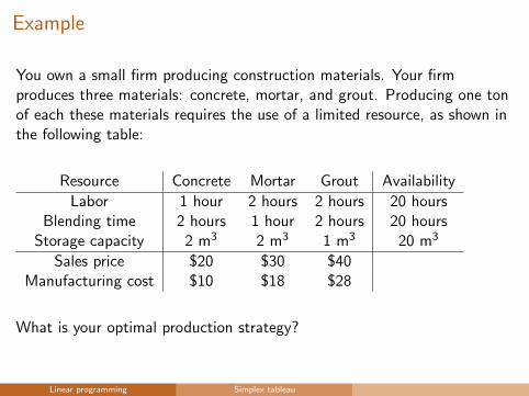
You own a small firm producing construction materials. Your firmproduces three materials: concrete, mortar, and grout. Producing one tonof each these materials requires the use of a limited resource, as shown inthe following table:

Resource Concrete Mortar Grout Availability

Labor 1 hour 2 hours 2 hours 20 hoursBlending time 2 hours 1 hour 2 hours 20 hours

Storage capacity 2 m3 2 m3 1 m3 20 m3

Sales price $20 $30 $40Manufacturing cost $10 $18 $28

What is your optimal production strategy?

Linear programming Simplex tableau

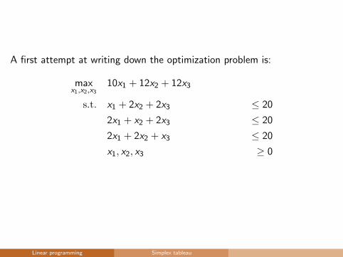
A first attempt at writing down the optimization problem is:

maxx1,x2,x3

10x1 + 12x2 + 12x3

s.t. x1 + 2x2 + 2x3 ≤ 20

2x1 + x2 + 2x3 ≤ 20

2x1 + 2x2 + x3 ≤ 20

x1, x2, x3 ≥ 0


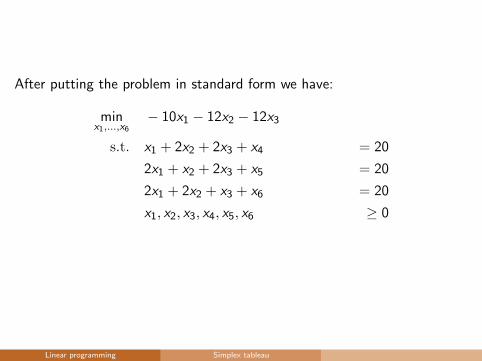
After putting the problem in standard form we have:

minx1,...,x6

− 10x1 − 12x2 − 12x3

s.t. x1 + 2x2 + 2x3 + x4 = 20

2x1 + x2 + 2x3 + x5 = 20

2x1 + 2x2 + x3 + x6 = 20

x1, x2, x3, x4, x5, x6 ≥ 0


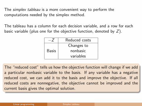
The simplex tableau is a more convenient way to perform thecomputations needed by the simplex method.

The tableau has a column for each decision variable, and a row for eachbasic variable (plus one for the objective function, denoted by Z ).

−Z Reduced costs

Changes toBasis nonbasic

variables

The “reduced cost” tells us how the objective function will change if we adda particular nonbasic variable to the basis. If any variable has a negativereduced cost, we can add it to the basis and improve the objective. If allreduced costs are nonnegative, the objective cannot be improved and thecurrent basis gives the optimal solution.


−Z Reduced costs

Changes toBasis nonbasic

variables

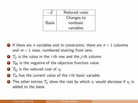
1 If there are n variables and m constraints, there are n + 1 columnsand m + 1 rows, numbered starting from zero.

2 Tij is the value in the i-th row and the j-th column.

3 T00 is the negative of the objective function value.

4 T0j is the reduced cost of xj .

5 Ti0 has the current value of the i-th basic variable.

6 The other entries Tij show the rate by which xi would decrease if xj isadded to the basis.


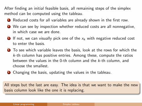
After finding an initial feasible basis, all remaining steps of the simplexmethod can be computed using the tableau.

1 Reduced costs for all variables are already shown in the first row.

2 We can see by inspection whether reduced costs are all nonnegative,in which case we are done.

3 If not, we can visually pick one of the xk with negative reduced costto enter the basis.

4 To see which variable leaves the basis, look at the rows for which thek-th column has positive entries. Among these, compute the ratiosbetween the values in the 0-th column and the k-th column, andchoose the smallest.

5 Changing the basis, updating the values in the tableau.

All steps but the last are easy. The idea is that we want to make the newbasis column look like the one it is replacing.


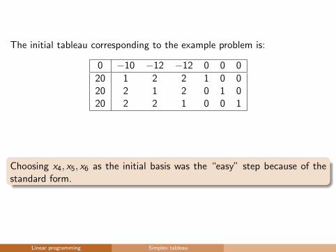
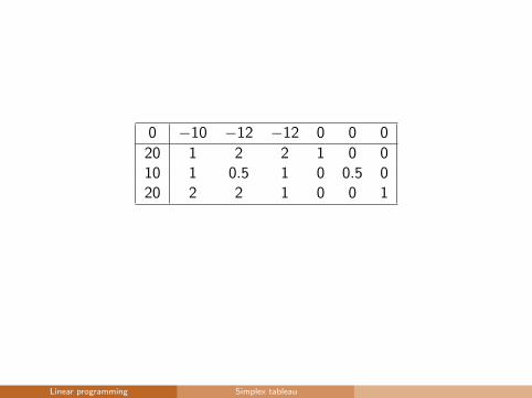
The initial tableau corresponding to the example problem is:

0 −10 −12 −12 0 0 0

20 1 2 2 1 0 020 2 1 2 0 1 020 2 2 1 0 0 1

Choosing x4, x5, x6 as the initial basis was the “easy” step because of thestandard form.


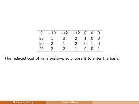
0 −10 −12 −12 0 0 0

20 1 2 2 1 0 020 2 1 2 0 1 020 2 2 1 0 0 1

The reduced cost of x1 is positive, so choose it to enter the basis.


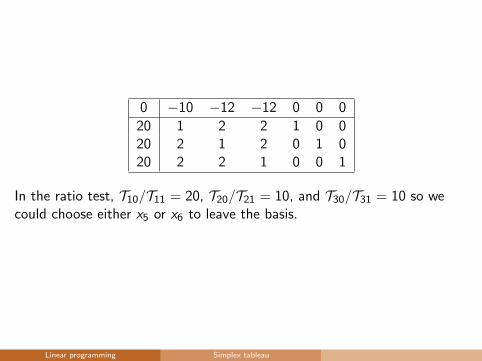
0 −10 −12 −12 0 0 0

20 1 2 2 1 0 020 2 1 2 0 1 020 2 2 1 0 0 1

In the ratio test, T10/T11 = 20, T20/T21 = 10, and T30/T31 = 10 so wecould choose either x5 or x6 to leave the basis.


Since x1 is entering the basis and x5 is leaving, we want to make columnx1 of the tableau look like x5 does currently.

We accomplish this with the following matrix row manipulations(performed in this order):

Divide every element in the second row by 2.

Add ten times the second row to the zero-th row.

Subtract the second row from the first row.

Subtract twice the second row from the third row.


0 −10 −12 −12 0 0 0

20 1 2 2 1 0 010 1 0.5 1 0 0.5 020 2 2 1 0 0 1


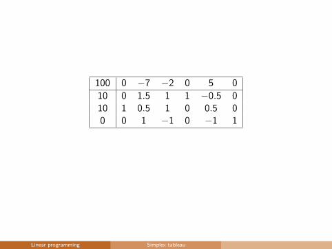
100 0 −7 −2 0 5 0

10 0 1.5 1 1 −0.5 010 1 0.5 1 0 0.5 00 0 1 −1 0 −1 1


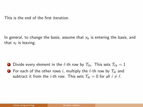
This is the end of the first iteration.

In general, to change the basis, assume that xk is entering the basis, andthat x` is leaving.

1 Divide every element in the `-th row by T`k . This sets T`k = 1

2 For each of the other rows i , multiply the `-th row by Tik andsubtract it from the i-th row. This sets Tik = 0 for all i 6= `.


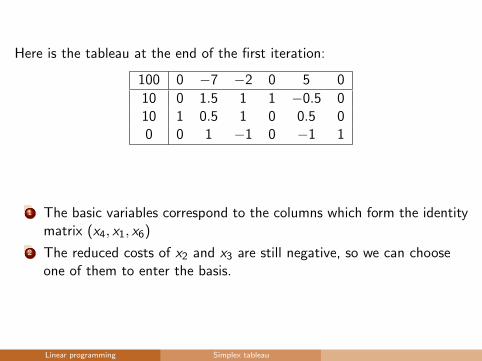
Here is the tableau at the end of the first iteration:

100 0 −7 −2 0 5 0

10 0 1.5 1 1 −0.5 010 1 0.5 1 0 0.5 00 0 1 −1 0 −1 1

1 The basic variables correspond to the columns which form the identitymatrix (x4, x1, x6)

2 The reduced costs of x2 and x3 are still negative, so we can chooseone of them to enter the basis.


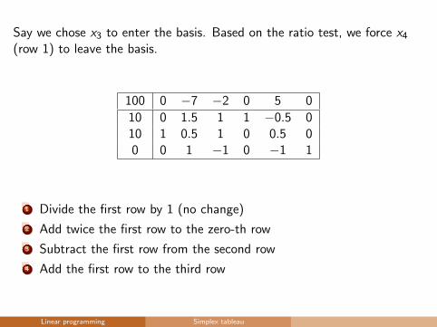
Say we chose x3 to enter the basis. Based on the ratio test, we force x4

(row 1) to leave the basis.

100 0 −7 −2 0 5 0

10 0 1.5 1 1 −0.5 010 1 0.5 1 0 0.5 00 0 1 −1 0 −1 1

1 Divide the first row by 1 (no change)

2 Add twice the first row to the zero-th row

3 Subtract the first row from the second row

4 Add the first row to the third row


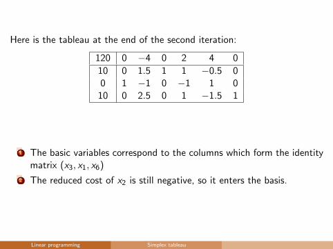
Here is the tableau at the end of the second iteration:

120 0 −4 0 2 4 0

10 0 1.5 1 1 −0.5 00 1 −1 0 −1 1 0

10 0 2.5 0 1 −1.5 1

1 The basic variables correspond to the columns which form the identitymatrix (x3, x1, x6)

2 The reduced cost of x2 is still negative, so it enters the basis.


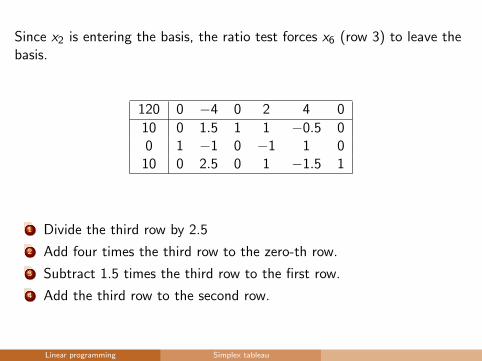
Since x2 is entering the basis, the ratio test forces x6 (row 3) to leave thebasis.

120 0 −4 0 2 4 0

10 0 1.5 1 1 −0.5 00 1 −1 0 −1 1 0

10 0 2.5 0 1 −1.5 1

1 Divide the third row by 2.5

2 Add four times the third row to the zero-th row.

3 Subtract 1.5 times the third row to the first row.

4 Add the third row to the second row.


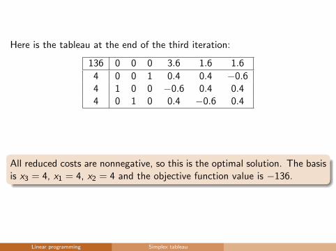
Here is the tableau at the end of the third iteration:

136 0 0 0 3.6 1.6 1.6

4 0 0 1 0.4 0.4 −0.64 1 0 0 −0.6 0.4 0.44 0 1 0 0.4 −0.6 0.4

All reduced costs are nonnegative, so this is the optimal solution. The basisis x3 = 4, x1 = 4, x2 = 4 and the objective function value is −136.


The only row operations which are allowed in the simplex tableau are:

Multiplying the pivot row by a positive constant.

Adding a multiple of the pivot row to another row.

(In matrix algebra, other row operations are used in solving systems oflinear equations, but they cannot be applied here.)


ODDS AND ENDS

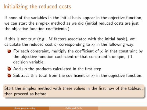
Initializing the reduced costs

If none of the variables in the initial basis appear in the objective function,we can start the simplex method as we did (initial reduced costs are justthe objective function coefficients.)

If this is not true (e.g., M factors associated with the initial basis), wecalculate the reduced cost c i corresponding to xi in the following way:

1 For each constraint, multiply the coefficient of xi in that constraint bythe objective function coefficient of that constraint’s unique, +1decision variable.

2 Add up the products calculated in the first step.

3 Subtract this total from the coefficient of xi in the objective function.

Start the simplex method with these values in the first row of the tableau,then proceed as before.

Linear programming Odds and Ends

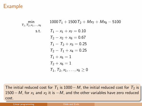
Example

minT1,T2,x1,...,x8

1000T1 + 1500T2 + Mx7 + Mx8 − 5100

s.t. T1 − x1 + x7 = 0.10

T2 − x2 + x8 = 0.67

T1 − T2 + x3 = 0.25

T2 − T1 + x4 = 0.25

T1 + x5 = 1

T2 + x6 = 1

T1,T2, x1, . . . , x8 ≥ 0

The initial reduced cost for T1 is 1000−M, the initial reduced cost for T2 is1500−M, for x1 and x2 it is −M, and the other variables have zero reducedcost.


A few checks

Basic variables should always have a zero reduced cost.

The columns of the tableau corresponding to the basis should form an“identity matrix” (all zeroes except for one ‘1’, each ‘1’ in a differentrow).

The values of the basic variables should always be nonnegative.


Which variable should enter the basis next?

Method 1: Pick the first variable with a negative reduced cost. (Pro: verysimple, provable convergence; Con: may not be a very good variable toenter)

Method 2: Pick the variable with the most negative reduced cost. (Pro:gives the greatest rate of increase in the objective; Con: you may not beable to move very far in this direction)

Method 3: Pick the variable which will decrease the objective the most(reduced cost times value of new basic variable). (Pro: gives themaximum increase in the objective per iteration; Con: takes morecalculation to pick the right variable.)

For large-scale, practical problems Method 1 is often sufficient; the extracomputation time required for Methods 2 and 3 is not worth it.


Computational complexity of the simplex method

In the worst case, the simplex method requires an exponential number ofsteps in the number of decision variables and constraints.

However, in practice it works quite well. (This is one place where thebig-O notation can be misleading for practical problems.)

Other “interior point” algorithms have polynomial complexity and arecompetitive with the simplex method.


Documents

Linear programming - GitHub Pages · The simplex method does exactly this. Starting from any extreme point, the method moves along the edges of the feasible region to form a sequence