Embed Size (px)
Citation preview
LINEAR PREDICTION FOR SINGLE SNAPSHOT MULTIPLE TARGET DOPPLER ESTIMATION UNDER POSSIBLY MOVING RADAR CLUTTER
A THESIS SUBMITTED TO THE GRADUATE SCHOOL OF NATURAL AND APPLIED SCIENCES
OF MIDDLE EAST TECHNICAL UNIVERSITY
BY
BAHA BARAN ÖZTAN
IN PARTIAL FULFILLMENT OF THE REQUIREMENTS FOR
THE DEGREE OF MASTER OF SCIENCE IN
ELECTRICAL AND ELECTRONICS ENGINEERING
JULY 2008
Approval of the thesis:
LINEAR PREDICTION FOR SINGLE SNAPSHOT MULTIPLE TARGET DOPPLER ESTIMATION UNDER POSSIBLY MOVING RADAR CLUTTER submitted by BAHA BARAN ÖZTAN in partial fulfillment of the requirements for the degree of Master of Science in Electrical and Electronics Engineering Department, Middle East Technical University by, Prof. Dr. Canan Özgen ____________ Dean, Graduate School of Natural and Applied Sciences Prof. Dr. İsmet Erkmen ____________ Head of Department, Electrical and Electronics Engineering Prof. Dr. Yalçın Tanık ____________ Supervisor, Electrical and Electronics Engineering Dept., METU Examining Committee Members: Prof. Dr. Mete Severcan _________________ Electrical and Electronics Engineering Dept., METU Prof. Dr. Yalçın Tanık _________________ Electrical and Electronics Engineering Dept., METU Assoc. Prof. Dr. Sencer Koç _________________ Electrical and Electronics Engineering Dept., METU Assist. Prof. Dr. Arzu Tuncay Koç _________________ Electrical and Electronics Engineering Dept., METU Dr. Mert Serkan _________________ Radar SMM – REHİS, ASELSAN
Date: 30.07.2008

I hereby declare that all information in this document has been obtained and presented in accordance with academic rules and ethical conduct. I also declare that, as required by these rules and conduct, I have fully cited and referenced all materials and results that are not original to this work.
Name, Last name : Baha Baran ÖZTAN
Signature :
iii
ABSTRACT
LINEAR PREDICTION FOR SINGLE SNAPSHOT MULTIPLE TARGET DOPPLER ESTIMATION UNDER POSSIBLY MOVING RADAR CLUTTER
Öztan, Baha Baran
M.S., Department of Electrical and Electronics Engineering
Supervisor : Prof. Dr. Yalçın Tanık
July 2008, 104 pages
We have devised a processor for pulsed Doppler radars for multi-target detection in
same folded range under land and moving clutter. To this end, we have investigated
the estimation of parameters, i.e., frequencies, amplitudes, and phases, of complex
exponentials that model target echoes under radar clutter characterized by antenna
scanning modulation with observation limited to single snapshot, i.e., one burst. The
Maximum Likelihood method of estimation is presented together with the bounds on
estimates, i.e., Cramér-Rao bounds. We have analyzed linear prediction, together
with its efficient implementation invented by Tufts & Kumaresan, and compared its
performance to other high resolution frequency estimation algorithms all modified to
run under clutter. The essential part of the work is that line spectra estimation
techniques model the clutter process also as a complex exponential. In addition,
linear prediction combined with linear time–invariant maximum Signal to
Interference Ratio (SIR) processor is analyzed. A technique to determine the model
order, which is required by the frequency estimation algorithms, is presented that
does not distinguish between targets and clutter. Clutter region concept is introduced
to identify targets from clutter. The possibility to use these algorithms for target
iv

classification is briefly explained after providing a literature survey on helicopter
echoes.
Keywords: Linear Prediction, Radar Clutter, Single Snapshot, Frequency Estimation.
v
ÖZ
DOĞRUSAL ÖNGÖRÜNÜN TEK GÖZLEM VE HAREKETLİ OLABİLEN RADAR KARGAŞASI ALTINDA BİRDEN FAZLA HEDEFİN DOPPLER
KESTİRİMİ İÇİN KULLANILMASI
Öztan, Baha Baran
Yüksek Lisans, Elektrik ve Elektronik Mühendisliği Bölümü
Tez Yöneticisi : Prof. Dr. Yalçın Tanık
Temmuz 2008, 104 sayfa
Darbeli Doppler radarlarında aynı katlanmış menzildeki birden çok hedefi, kara
kargaşası ve hareketli kargaşa altında tespit edecek bir yapı geliştirilmiştir. Bu
kapsamda radar tarafından tespit edilen hedefleri modelleyen birden fazla karmaşık
üstel işaretin frekans, genlik ve fazlarının kestirimi, bir darbe grubunu kapsayan tek
gözlem altında ve anten taraması kiplenimi ile şekillenen radar kargaşası varlığında
incelenmiştir. En büyük olabilirlik kestirimi yöntemi belirtilmiş ve frekans ile genlik
ve fazdan oluşan karmaşık çarpan için Cramér-Rao yansız kestirim değişinti alt
sınırları çıkartılmıştır. Doğrusal öngörü yöntemi, Tufts & Kumaresan tarafından
geliştirilen verimli uygulanışı ile birlikte, diğer yüksek çözünürlüklü frekans
kestirimi yöntemleri ile karşılaştırılarak ve radar kargaşası için gerekli değişikliler
yapılarak analiz edilmiştir. Çalışmamızın önemli özelliği, kullanılan yüksek
çözünürlüklü çizgisel spektrum kestirim yöntemlerinin radar kargaşasını da bir
karmaşık üstel işlev olarak modellemesidir. Doğrusal öngörü yönteminden önce
uygulanabilecek sinyalin kargaşa ve gürültüden oluşan toplam enterferansa olan güç
oranını (SIR) en yüksek değere çıkartan doğrusal zamanda değişmez filtrenin
başarımı ortaya konmuştur. Algoritmalara girdi olarak verilen model derecesini
vi

bulmak için hedef ve kargaşa ayrımı yapmayan bir teknik geliştirilmiştir. Kargaşa
bölgesi kavramı, hedefleri kargaşadan ayırmak için oluşturulmuştur. İncelenen
algoritmaların hedef sınıflandırma probleminde kullanımı, helikopter ekosu ile ilgili
literatür incelemesi verildikten sonra kısaca aktarılmıştır.
Anahtar Kelimeler: Doğrusal Öngörü, Radar Kargaşası, Tek Gözlem, Frekans
Kestirimi.
vii

viii
To My Parents
ACKNOWLEDGMENTS
The author wishes to express his deepest gratitude to his supervisor Prof. Dr.
Yalçın Tanık for his guidance, advice, criticism, encouragement, and insight
throughout the research.
The author would like to thank the members of the Radar Signal Processing
Research Team at METU supported by ASELSAN Inc. for their contribution in
establishing the author’s background in the area. The technical discussions with Prof.
Dr. Yalçın Tanık, Prof. Dr. Mete Severcan, Prof. Dr. Fatih Canatan, Assoc. Prof. Dr.
Sencer Koç, Assist. Prof. Dr. Ali Özgür Yılmaz, Assist. Prof. Dr. Çağatay Candan,
and Dr. Ülkü Çilek Doyuran are gratefully acknowledged. The author appreciates the
opportunity presented by ASELSAN Inc. for him to become a member of the
aforementioned research team. For her suggestions and comments, Dr. Ülkü Çilek
Doyuran is particularly appreciated.
The author would also like to thank for the scholarship received from the
Scientific and Technological Research Council of Turkey (TÜBİTAK) during the
course of master’s studies.
Lastly, the author believes that the support of his parents and the friendship of
his colleague Gökhan Muzaffer Güvensen have to be honored.
ix
TABLE OF CONTENTS
ABSTRACT................................................................................................................ iv
ÖZ ............................................................................................................................... vi
ACKNOWLEDGMENTS .......................................................................................... ix
TABLE OF CONTENTS............................................................................................. x
LIST OF TABLES ....................................................................................................xiii
LIST OF FIGURES .................................................................................................. xiv
CHAPTERS
1. INTRODUCTION.................................................................................................... 1
1.1. Nomenclature .................................................................................................... 3
2. SIGNAL MODEL.................................................................................................... 5
3. RADAR DETECTORS, DOPPLER PROCESSORS AND OPTIMAL
APPROACH .............................................................................................................. 11
3.1. Conventional Radar Processors....................................................................... 11
3.2. Maximum Likelihood (ML) Technique .......................................................... 13
3.3. Cramér-Rao Bound ......................................................................................... 16
4. LINEAR PREDICTION AND THE TUFTS–KUMARESAN METHOD ........... 17
4.1. Motivation ....................................................................................................... 17
4.2. Linear Prediction............................................................................................. 18
4.2.1. Further Remarks on Linear Prediction..................................................... 20
4.3. Modified Tufts-Kumaresan Method ............................................................... 21
4.3.1. Overview of Tufts-Kumaresan Method ................................................... 21
4.3.2. Tufts-Kumaresan Algorithm Details........................................................ 22
4.3.3. FBTK, FTK vs. BTK in Modeling Clutter............................................... 26
4.3.4. FBTK Noise Reduced Data Vector Version ............................................ 27
4.4. Distinguishing Clutter and Targets: the Concept of Clutter Region ............... 27
4.5. Linear Predictor as a Radar Processor ............................................................ 27
x
5. OTHER HIGH RESOLUTION LINE SPECTRA ESTIMATION TECHNIQUES
.................................................................................................................................... 30
5.1. Can Pure DFT Be an Alternative? .................................................................. 30
5.2. MUSIC Algorithm .......................................................................................... 32
5.2.1. Basic MUSIC Algorithm ......................................................................... 32
5.2.2. Estimation of the Autocorrelation Matrix from Single Snapshot
Observation ........................................................................................................ 33
5.2.3. MUSIC Algorithm as Applied to Our Problem ....................................... 35
5.3. Use of MUSIC Technique in the Literature.................................................... 37
5.4. Total Least Squares ESPRIT Algorithm......................................................... 38
5.4.1. Basic Total Least Squares ESPRIT Algorithm........................................ 38
5.4.2. Total Least Squares ESPRIT Algorithm as Applied to Our Problem...... 38
5.5. High Resolution Methods Combined with ML............................................... 40
6. DETERMINATION OF AMPLITUDES AND PHASES..................................... 42
6.1. Least Squares Estimator .................................................................................. 42
6.2. Maximum Likelihood Derivative Equations................................................... 43
6.3. Comparison of Techniques ............................................................................. 43
7. CLUTTER REGIONS AND DETERMINATION OF THE NUMBER OF
SIGNAL PLUS CLUTTER ZEROS.......................................................................... 44
8. LTI MAXSIR FILTER DESIGN FOR LAND CLUTTER................................... 59
9. SIMULATION RESULTS .................................................................................... 62
9.1. Simulation Parameters .................................................................................... 62
9.2. Selection of the Superior Algorithms.............................................................. 64
9.3. Analysis of Linear Prediction and FBTK Algorithm...................................... 66
9.4. Effect of SNR for the Selected Algorithms..................................................... 73
9.5. Frequency Resolution for the Selected Algorithms ........................................ 78
9.6. LTI MAXSIR Filter and FBTK Method......................................................... 83
9.7. Concluding Comments on Simulation Results ............................................... 84
10. FURTHER APPLICATIONS OF HIGH RESOLUTION LINE SPECTRAL
ANALYSIS METHODS IN RADARS ..................................................................... 85
10.1. Moving Clutter .............................................................................................. 85
10.2. Target Discrimination ................................................................................... 86
xi
xii
10.2.1. Modeling Helicopter Echo ..................................................................... 87
10.2.2. Proposed Classification Method ............................................................ 87
11. CONCLUSION AND FUTURE WORKS .......................................................... 88
REFERENCES........................................................................................................... 91
APPENDICES
A. IMPLEMENTATION OF MAXIMUM LIKELIHOOD TECHNIQUE.............. 97
B. LITERATURE ON HELICOPTER ECHO AND DETECTION AND
CLASSIFICATION ................................................................................................. 100
B.1. Body (Fuselage, Skin) .................................................................................. 100
B.2. Main Rotor.................................................................................................... 100
B.3. Tail Rotor...................................................................................................... 102
B.4. Hub ............................................................................................................... 102
B.5. Some of the Other Available Techniques..................................................... 104

LIST OF TABLES
TABLES
Table 1 Distribution of number of detections for various SNR levels, CNR=45dB . 63
Table 2 Performance of all the algorithms for the selected operating condition ....... 65
xiii
LIST OF FIGURES
FIGURES
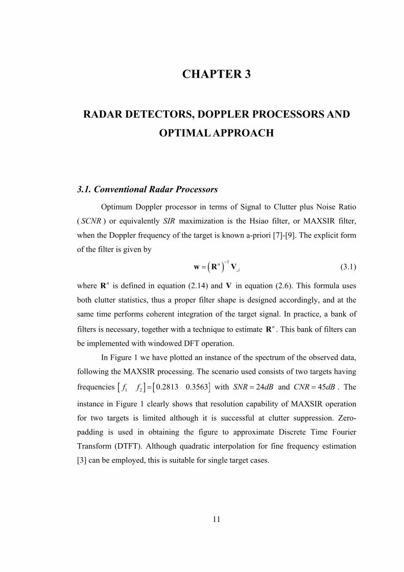
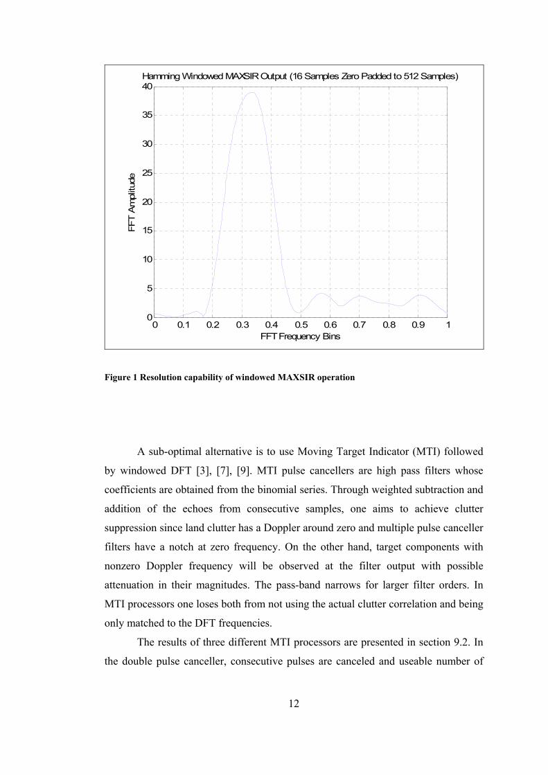
Figure 1 Resolution capability of windowed MAXSIR operation............................. 12
Figure 2 Linear prediction block diagram.................................................................. 18
Figure 3 Forward and backward linear prediction ..................................................... 18
Figure 4 Relationship between linear prediction and AR processes.......................... 20
Figure 5 Zeros of prediction-error filter..................................................................... 26
Figure 6 DTFT analysis of input data ........................................................................ 31
Figure 7 MUSIC spectrum......................................................................................... 37
Figure 8 Log-likelihood function for a sample data for CNR=50dB......................... 41
Figure 9 Complex multiplier estimates of FBTK when no targets are present,
CNR=25dB................................................................................................................. 48
Figure 10 Frequency estimates of FBTK when no targets are present, CNR=25dB . 49
Figure 11 Complex multiplier estimates of FBTK when no targets are present,
CNR=50dB................................................................................................................. 50
Figure 12 Frequency estimates of FBTK when no targets are present, CNR=50dB . 51
Figure 13 Complex multiplier estimates of FBTK when no targets are present,
CNR=100dB............................................................................................................... 52
Figure 14 Frequency estimates of FBTK when no targets are present with a zoomed
in view provided to show the determination of the clutter region width, CNR=100dB
.................................................................................................................................... 53
Figure 15 Complex multiplier estimates of FBTK, CNR=50dB, SNR=24dB........... 54
Figure 16 Frequency estimates of FBTK, CNR=50dB, SNR=24dB ......................... 55
Figure 17 Complex multiplier estimates of FBTK, CNR=50dB, infinite SNR case . 56
Figure 18 Frequency estimates of FBTK, CNR=50dB, infinite SNR case................ 57
Figure 19 LTI MAXSIR filters of different orders .................................................... 61
Figure 20 Bias of linear prediction when clutter plus noise autocorrelation is known
.................................................................................................................................... 67
xiv
Figure 21 Standard deviation of FBTK frequency estimates for different filter orders,
................................................................................................................................ 68 L
Figure 22 Bias of FBTK frequency estimates for different filter orders, .............. 69 L
Figure 23 Standard deviation of FBTK frequency estimates in comparison to CR
bound for increasing number of samples (SNR increases with increasing number of
samples) ..................................................................................................................... 70
Figure 24 Standard deviation of FBTK frequency estimates in comparison to CR
bound for increasing number of samples (SNR is kept fixed) ................................... 71
Figure 25 Standard deviation of FBTK frequency estimates as a function of number
of samples (Prediction order increases with number of samples as 9, 18, 36, 72). ... 72
Figure 26 Standard deviation of FBTK frequency estimates as a function of number
of samples (Prediction order increases with number of samples as 9, 25, 57, 121). . 73
Figure 27 Standard deviation of the first target’s frequency estimate of selected
methods with SNR ..................................................................................................... 74
Figure 28 Bias of the first target’s frequency estimate of selected methods with SNR
.................................................................................................................................... 75
Figure 29 RMS value of separation of the first target’s estimated and actual complex
multiplier with SNR for selected methods (Least squares method)........................... 76
Figure 30 RMS value of separation of the first target’s estimated and actual complex
multiplier with SNR for selected methods (Maximum likelihood method) .............. 77
Figure 31 Bias of the first target’s estimated and actual complex multiplier with SNR
for selected methods (Maximum likelihood method) ................................................ 78
Figure 32 Standard deviation of frequency estimate of selected methods with change
in Doppler frequency of the first target...................................................................... 79
Figure 33 Bias of frequency estimate of selected methods with change in Doppler
frequency of the first target ........................................................................................ 80
Figure 34 RMS value of separation of estimated and actual complex multiplier with
change in Doppler frequency of the first target for selected methods (Least squares
method) ...................................................................................................................... 81
Figure 35 RMS value of separation of estimated and actual complex multiplier with
change in Doppler frequency of the first target for selected methods (Maximum
likelihood method) ..................................................................................................... 82
xv
xvi
Figure 36 Bias of separation of estimated and actual complex multiplier with change
in Doppler frequency of the first target for selected methods (Maximum likelihood
method) ...................................................................................................................... 83
Figure 37 Standard deviation of the first target’s frequency estimate of FBTK
method preceded by LTI MAXSIR filter................................................................... 84
Figure 38 Zeros of prediction-error filter when two sources of clutter are present ... 86
Figure 39 Helicopter spectrum (For the hovering or zero radial velocity case, fbody=0,
otherwise fbody≠0)..................................................................................................... 103
Figure 40 Fixed-wing spectrum (For targets with zero radial velocity fbody=0,
otherwise fbody≠0)..................................................................................................... 104
CHAPTER 1
INTRODUCTION
Radar research mainly attracts researchers from the electromagnetics and
signal processing areas. Algorithm development for achieving certain tasks is one of
the main roles of the signal processing and communications oriented researchers.
Determination of targets, their number, radial velocity and if possible, their types
under strong radar clutter, received echoes from the natural environment land, sea,
and weather, have been the major concern of radar designers. Conventional methods
like MAXimum Signal to Interference Ratio (MAXSIR) and Moving Target
Indicator (MTI) processors, which are in fact clutter suppression filters followed by
Discrete Fourier Transformation (DFT), are developed with the aim of clutter
elimination, but they suffer from limited resolution capability when used on the radar
echo containing multiple targets in the same folded range. This is detailed in Chapter
3 where one can find the literature survey on the conventional radar processors.
In this work, we will study the applicability of Linear Prediction and high
resolution frequency estimation methods to the specified problem for land based
radars. The aforementioned methods were originally developed to run under Additive
White Gaussian Noise (AWGN). The main difference between the usual use of these
algorithms and their use in radar problem is the presence of clutter in the radar echo
in contrast to operation under AWGN. The clutter elimination is curial for the
success of radars and whether these algorithms can also model clutter and how to
supply these algorithms the total number of targets and clutter components are the
questions to be answered. Consequently, the high resolution frequency estimation
algorithms need certain modifications to be used for the multi-target Doppler tone
detection under radar clutter. Although separate works investigating the use of some
of the high resolution algorithms for different kinds of radars can be found in the
1
literature, they deserve a unified treatment, possibly including modifications, with all
versions of the selected frequency estimation algorithms concerned. Yet there
remains the task of distinguishing targets from clutter since the algorithms to be used
will treat the clutter and the targets in the same fashion not knowing their origin. This
thesis is conducted to find feasible answers to the aforementioned problems.
In this thesis work, we have thoroughly analyzed the use of Linear Prediction,
together with its efficient implementation invented by Tufts & Kumaresan [1], and
some other high resolution frequency estimation methods, namely, various versions
of MUltiple SIgnal Classification (MUSIC) and Estimation of Signal Parameters via
Rotational Invariance Techniques (ESPRIT) in radar processing, where the data is
corrupted with possibly multiple sources of clutter.
The core of the work is that line spectra estimation techniques can be used to
model the clutter as a sum of complex exponential terms, just as they model the
targets.
We will be analyzing the estimation of parameters, i.e., frequencies,
amplitudes, and phases, of complex exponentials that model target echoes under
radar land and possibly moving clutter characterized by the antenna scanning
modulation effect. The observation will be limited to a single snapshot, i.e., one burst.
Optimal method of estimation, which is the Maximum Likelihood technique, will be
presented in its various forms together with the bounds on estimates, i.e., Cramér-
Rao bounds. These bounds will serve as the ultimate performances of the algorithms
we will test.
A technique to determine the model order required by all of the high
resolution frequency estimation methods will be presented that does not distinguish
between the targets and the clutter. The proposed clutter region concept is then used
to identify the targets from the clutter.
In addition, linear predictor combined with Linear Time–Invariant (LTI)
maximum Signal to Interference Ratio ( SIR ) filter is investigated.
Lastly, a literature survey on helicopter echoes and detection is provided to
access the possibility to use Linear Prediction (LP) for target classification.
2
We have published our preliminary works in [2]. The literature survey on
various parts of the work in relation to the radar problem will be presented after the
explanation of the corresponding parts.
We present the signal model in Chapter 2; conventional radar processors will
be presented followed by the optimum nonrandom parameter estimation technique of
Maximum Likelihood and derived Cramér-Rao bounds in Chapter 3. Chapter 4
focuses on linear prediction and Tufts-Kumaresan algorithm together with their use
in radars. Chapter 5 deals with the modification of selected line spectra estimation
algorithms to be used in radars and a different implementation of Maximum
Likelihood technique that needs to be preceded by a high resolution frequency
estimation algorithm. Determination of amplitudes and phases of targets will be
discussed in Chapter 6, where a brief comparison of the algorithms is also presented.
The clutter region concept first introduced in Chapter 4 will be further elaborated
together with the model order determination procedure in Chapter 7. We will develop
the LTI MAXSIR filter that can precede a high resolution spectra estimation
algorithm under scenarios containing land clutter in Chapter 8. In Chapter 9, we
present the performances of the algorithms through Monte-Carlo simulations. In
Chapter 10, the concepts developed are extended to moving clutter problem, where
the only difference assumed is the center frequency shift of the clutter. Target
classification based on LP and other high resolution frequency estimation algorithms
is also included in this chapter.
1.1. Nomenclature
In this section notations and some of the conventions used throughout the
thesis will be given.
A denotes a matrix, denotes a vector, denotes the a :, jA thj column of
matrix , denotes the element at the row and A ,k jΑ thk thj column of matrix and
denotes the
A
ja thj element of vector a . { }E i is the expectation operator. Some of
the upper-right corner signs and their meanings are as follows: * : conjugation, ' : derivative,
3

T : transpose, H : hermitian, and # : pseudoinverse operator.
“Signal” can both mean the complete signal model explained in the following
chapter, or, the part modeling the targets, which will be clear from the context.
Throughout this thesis work it is assumed that eigenvalues of all matrices are
ordered in decreasing order.
4
CHAPTER 2
SIGNAL MODEL
In this chapter the model of the radar echo that will be used in target detection
and high resolution velocity estimation will be explained in detail.
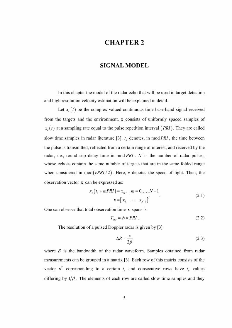
Let ( )cx t be the complex valued continuous time base-band signal received
from the targets and the environment. x consists of uniformly spaced samples of
( )cx t at a sampling rate equal to the pulse repetition interval ( )PRI
PRI
. They are called
slow time samples in radar literature [3]. denotes, in mod , the time between
the pulse is transmitted, reflected from a certain range of interest, and received by the
radar, i.e., round trip delay time in mod . is the number of radar pulses,
whose echoes contain the same number of targets that are in the same folded range
when considered in mod ( . Here, c denotes the speed of light. Then, the
observation vector can be expressed as:
ot
PRI N
)
1
/ 2cPRI
x
( )
[ ]0 1
, 0, ,c o m
TN
x t mPRI x m N
x x −
+ = = −
=x
…. (2.1)
One can observe that total observation time x spans is
obsT N PRI= × . (2.2)
The resolution of a pulsed Doppler radar is given by [3]
2cRβ
Δ = (2.3)
where β is the bandwidth of the radar waveform. Samples obtained from radar
measurements can be grouped in a matrix [3]. Each row of this matrix consists of the
vector corresponding to a certain and consecutive rows have values
differing by
Tx ot ot
1 β . The elements of each row are called slow time samples and they
5
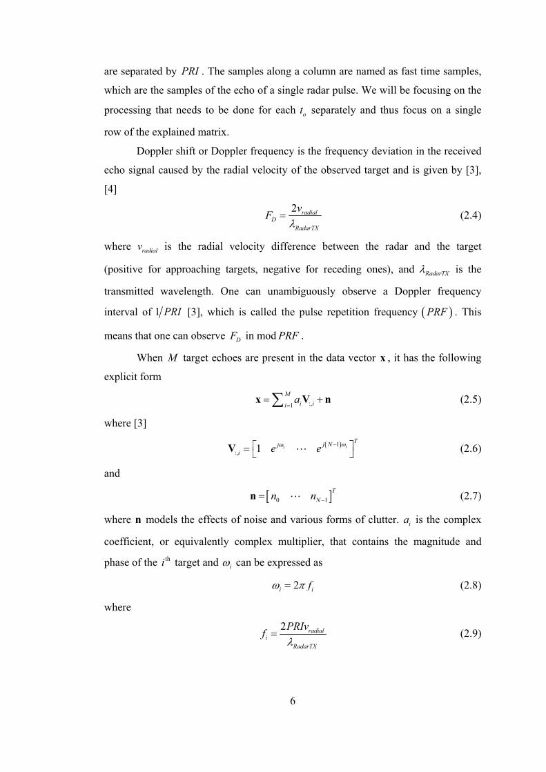
are separated by PRI . The samples along a column are named as fast time samples,
which are the samples of the echo of a single radar pulse. We will be focusing on the
processing that needs to be done for each separately and thus focus on a single
row of the explained matrix.
ot
Doppler shift or Doppler frequency is the frequency deviation in the received
echo signal caused by the radial velocity of the observed target and is given by [3],
[4]
2 radial
Rada
vD
rTX
Fλ
= (2.4)
where is the radial velocity difference between the radar and the target
(positive for approaching targets, negative for receding ones), and
radialv
RadarTXλ is the
transmitted wavelength. One can unambiguously observe a Doppler frequency
interval of 1 PRI ) [3], which is called the pulse repetition frequency ( . This
means that one can observe
PRF
DF in mod . PRF
When M target echoes are present in the data vector x , it has the following
explicit form
:,a1
Mi ii=
= +∑x V n (2.5)
where [3]
( )1:, 1 ii
Tj Nji e e ωω −⎡ ⎤= ⎣ ⎦V (2.6)
and
[ ]0 1T
Nn n −=n (2.7)
where models the effects of noise and various forms of clutter. is the complex
coefficient, or equivalently complex multiplier, that contains the magnitude and
phase of the target and
n ia
thi iω can be expressed as
2i fiω π= (2.8)
where
2 radiali
Rada
PRIv
rTX
fλ
= (2.9)
6
Note that, in equation (2.9), is given in modradialv 2RadarTX
PRIλ⎛⎜⎝ ⎠
⎞⎟ . Our aim is to
decide on M and to estimate and ia if for each target.
ia has a random phase which is uniformly distributed in [ )0, 2π . ia is
another random variable with a proper distribution. Note that, with this notation we
have implicitly assumed that attains the same value from pulse-to-pulse and can
change from scan-to-scan. This corresponds to Swerling models of 1 or 3 depending
on the distribution of
ia
2ia one uses to model target echoes [3].
In our work, the phases of the targets are modeled by taking them as
independent identically distributed random variables with ia∠ , phase of , being a
uniformly distributed random variable in
ia
[ )0, 2π . ia is considered as an unknown
parameter (nonrandom, i.e., its probability distribution is not known). The necessary
derivations will include the cases of ia∠ being nonrandom and being random
although the latter is used in the simulations to obtain numerical results.
One can obtain the results for various values of , 1, ,ia i M= … to obtain the
conditional probability density function of a desired quantity z , which can be a
frequency or complex multiplier estimate, as ( )1 Mp z a a and the generalization
to the random magnitude case is trivial with the integral
( ) ( ) ( )1 1 1d dM M Mp z p z a a p a a a a= ∫ (2.10)
where ( 1 M )p a a is the probability density function one decides to use for the
magnitudes of the targets and ( )p z is the probability density function of the desired
quantity under this condition. z
In summary, throughout this work, the assumed probability density function
of in polar coordinates is ia
( ) (12ia
i)ip r r
aδ
π= − a . (2.11)
The normalized frequency of a target if is also taken as a nonrandom
parameter.
7
Noise and clutter together can be treated as a colored noise and n is the
corresponding vector modeling complex Gaussian white noise with identically
distributed real and imaginary parts and the clutter components. Clutter components
can be of two types: land clutter and moving (weather etc.) clutter. The composite
clutter is assumed to be of complex circularly symmetric Gaussian distribution. This
makes sense since radar echoes from individual resolution volumes are the
superposition of scattered echoes by a large number of particles, forming a Gaussian
random process [5]. The governing equations for n are
{ }E =n 0 (2.12)
2
22
n LCWN NxN
WN
σσσ
⎛ ⎞= +⎜
⎝ ⎠R I RC
⎟ (2.13)
where
{ }*,
nk l k lE=R n n . (2.14)
2WNσ and 2
LCσ are the powers of the white noise and land clutter components,
respectively. is the total clutter autocorrelation matrix and includes land clutter
and optionally moving clutter components (normalized matrices and
CRLCR MCR ,
respectively).
2
2C LC MMC
LC
σσ
= +R R R C (2.15)
where 2MCσ is the power of the moving clutter. Elements of are obtained
considering antenna scanning modulation effect
LCR
[6], [4]. Due to angular motion of
the antenna in a mechanically scanned system, the radar does not receive echoes
from the identical patches of scatterers from consecutive pulses. This causes
degradation of the pulse-to-pulse clutter correlation. This effect can also be explained
in the following way. Due to finite time on clutter scatterers, the clutter spectrum
widens, i.e., loss of correlation is observed. The longer the time on clutter patch, the
less will be the spread in the clutter spectrum.
If the two-way antenna power pattern is approximated as a Gaussian pattern,
one obtains a Gaussian shaped clutter power spectrum [6] with the autocorrelation
8
matrix entries found using the fact that Fourier Transformation of a Gaussian
function is also Gaussian and given by
( )( )22
, exp2
wLCk l
k l PRIσ⎡ ⎤−⎢ ⎥= −⎢ ⎥⎣ ⎦
R (2.16)
where wσ is the standard deviation of the clutter power spectrum and given by [6]
( )
12
22272 ln 2
WHPw
θσ
α
−°⎡ ⎤
⎢ ⎥=⎢ ⎥⎣ ⎦
. (2.17)
In equation (2.17), is the two way half power beamwidth of the radar antenna
and
2WHPθ °
α is the rotation rate of the radar antenna in units revolutionsminute and
will be used to denote the value of
rpm
α . MCR is obtained through the equations
( )HMC MC LC MC=R D R D (2.18)
( )2 1, , 1, ,cj f kMC
k k e kπ −= =D … N (2.19)
where MCD is a diagonal matrix and cf is the moving clutter center frequency.
The equations (2.15), (2.18), and (2.19) are valid up to one moving clutter
source. For cases containing more than one moving clutter source the extension is
trivial. Until Chapter 10, it will be assumed that the only source of clutter is land
clutter.
As a final remark on the received signal model, note that clutter, noise, and
target components of the received signal are all taken as independent.
We will choose our definition in a way such that it reflects the effect of
and thus in comparison with previous works, one may need to be careful about
different conventions. SN for each target is defined as the SN when the other
target is not present and is given by
SNR
R
N
R
2
210 log ii
WN
a NSNR
σ
⎛ ⎞= ⎜
⎜⎝ ⎠
⎟⎟
. (2.20)
9

will refer to land clutter to white noise power ratio, i.e., CNR 2 2 to LC WNσ σ ,
and MCCR to moving clutter to land clutter power ratio, i.e., 2 2 to MC LCσ σ .
In some equations although the autocorrelation matrix may appear as defined
in this chapter, it may refer to a submatrix of the one defined in this chapter. It will
have an appropriate size, which will become clear from the equations.
For figures presented, please consult section 9.1. for further details on used
parameters.
10
CHAPTER 3
RADAR DETECTORS, DOPPLER PROCESSORS AND
OPTIMAL APPROACH
3.1. Conventional Radar Processors
Optimum Doppler processor in terms of Signal to Clutter plus Noise Ratio
( ) or equivalently SI maximization is the Hsiao filter, or MAXSIR filter,
when the Doppler frequency of the target is known a-priori
SCNR R
[7]-[9]. The explicit form
of the filter is given by
( ) 1
:,n
i
−=w R V (3.1)
where is defined in equation nR (2.14) and V in equation (2.6). This formula uses
both clutter statistics, thus a proper filter shape is designed accordingly, and at the
same time performs coherent integration of the target signal. In practice, a bank of
filters is necessary, together with a technique to estimate . This bank of filters can
be implemented with windowed DFT operation.
nR
In Figure 1 we have plotted an instance of the spectrum of the observed data,
following the MAXSIR processing. The scenario used consists of two targets having
frequencies [ ] [ ]1 2 0.2813 0.3563f f = with 24SNR dB= and . The
instance in
45CNR dB=
Figure 1 clearly shows that resolution capability of MAXSIR operation
for two targets is limited although it is successful at clutter suppression. Zero-
padding is used in obtaining the figure to approximate Discrete Time Fourier
Transform (DTFT). Although quadratic interpolation for fine frequency estimation
[3] can be employed, this is suitable for single target cases.
11
0 0.1 0.2 0.3 0.4 0.5 0.6 0.7 0.8 0.9 10
5
10
15
20
25
30
35
40
FFT
Am
plitu
de
Hamming Windowed MAXSIR Output (16 Samples Zero Padded to 512 Samples)
FFT Frequency Bins
Figure 1 Resolution capability of windowed MAXSIR operation
A sub-optimal alternative is to use Moving Target Indicator (MTI) followed
by windowed DFT [3], [7], [9]. MTI pulse cancellers are high pass filters whose
coefficients are obtained from the binomial series. Through weighted subtraction and
addition of the echoes from consecutive samples, one aims to achieve clutter
suppression since land clutter has a Doppler around zero and multiple pulse canceller
filters have a notch at zero frequency. On the other hand, target components with
nonzero Doppler frequency will be observed at the filter output with possible
attenuation in their magnitudes. The pass-band narrows for larger filter orders. In
MTI processors one loses both from not using the actual clutter correlation and being
only matched to the DFT frequencies.
The results of three different MTI processors are presented in section 9.2. In
the double pulse canceller, consecutive pulses are canceled and useable number of
12
output samples is one less than the number of input samples. This version is named
as HWMTI_11, where HW letters are added for Hamming Windowing after MTI
operation. Another version presented combines three samples with the coefficients 1,
-2, and 1 and called HWMTI_121. In this version, useable number of output samples
is two less than the number of input samples. In the third alternative, we use all the
output samples and use a combination of two and three pulse canceller. The input
vector is processed by the matrix
. (3.2)
1 1 0 01 2 1 0 00 00 0 00 0 1 2 10 0 1 NxN
−⎡ ⎤⎢ ⎥−⎢ ⎥⎢ ⎥⎢⎢ ⎥⎢ ⎥−⎢ ⎥
−⎣ ⎦
0
1
⎥
This last version is named as HWMTI.
3.2. Maximum Likelihood (ML) Technique
The generally accepted best procedure of frequency estimation is based on the
Maximum Likelihood (ML) method. If an unbiased estimator that attains the
Cramér-Rao bound (to be defined in the next section) exists, it is ML. For large ,
ML estimator has asymptotic properties of being unbiased, efficient, and Gaussian
distributed
N
[10].
Let us derive the ML equations for our problem of targets in radar clutter.
Assuming that is perfectly known, the conditional probability density function of
is
nR
x [10]
( ) { }( ) { }( )( )1 11| , , , , , exp
detH
M M N np a a E Eω ωπ
= − − −x xR
… x Q x x (3.3)
where
( ) 1n −=Q R (3.4)
and
{ } { }:,1
Mi ii
E a E=
= +∑x V n . (3.5)
13
The ML estimates of ’s and ia iω ’s can be obtained through the maximization
of equation (3.3), or equivalently
{ }( ) { }( )1 1, , , , ,
minM M
H
a aE
ω ω− −x x Q x x
… …E . (3.6)
Note that with expression (3.6), we have converted our cost function from p to
and maximization to minimization. ( )ln p−
The problem considered here is referred to as deterministic maximum
likelihood [11] in contrast to the case where the complex multipliers of the complex
exponentials are treated not as parameters, but as random variables. The latter
approach is called stochastic maximum likelihood [11].
Theorem [12]: Let ( )( )*ln ,p z z be a real-valued function of the complex
vectors and . The vector pointing in the direction of the maximum rate of
change of
z *z
( )( )*ln z z,p is ( )( )**ln ,p∇
zz z .
The scalar version of the complex gradient is given by [11]
( )( ) ( ) ( )*
* ln ln1ln ,2z
real imaginary
p pp z z j
z z⎛ ⎞∂ ∂
∇ = +⎜⎜ ∂ ∂⎝ ⎠⎟⎟ (3.7)
where
real imaginaryz z jz= + . (3.8)
When one uses the given definition of derivatives in solving the minimization
expression (3.6), the following governing equations are obtained from the
minimization with respect to ’s ka
:, :, :,10, 1, ,MH H
k k l lla k
=− + = = M∑V Qx V Q V … (3.9)
and from the minimization with respect to pω ’s
{ } { }* ' ':, :, :,1
2 Re 2 Re 0, 1, ,M H Hi p i p p pi
a a a p M=
− = =∑ V QV x QV … (3.10)
where
( ) ( )1':, 0 1p
Tjp je j N eω − pj N ω⎡ ⎤= −⎣ ⎦V . (3.11)
Although the general model can be developed assuming a nonzero mean for
the clutter and noise (together treated as a colored noise), in the subsequent parts we
14
will assume a zero mean since generally there is no reason to assume a nonzero mean
for the colored noise part of a radar observation.
One can observe that the ML estimates for ’s and ia iω ’s are unbiased by
taking the expected values of both sides of the equations (3.9) and (3.10). In other
words, expected values of estimates are found to be equal to their actual values.
Now, let us examine if there occurs any change in equations (3.9) and (3.10),
for the situation involving random target phases. There will be no change since for
any given parameter vector φ , one will do the maximization of the following
function
( ) ( ) ( )( ) ( ) (
|
ln ln | ln
p p p
p p
=
= +
x,φ x φ φ
x,φ x φ φ)p (3.12)
and
( )ln p∇ =⎡ ⎤⎣ ⎦φ φ 0 (3.13)
for uniform distribution on φ .
Note that ML equations (3.9) and (3.10) are such that given iω ’s, ’s can be
solved. Thus one can do the minimization only with respect to
ia
iω ’s. Defining
[ ]1T
Ma a=a (3.14)
the minimization problem (3.6) can be expressed as
( )12
1
2
, , ,min -
Mf f aQ x Va (3.15)
where
:,k k=V v . (3.16)
The minimization with respect to is obtained by a
( )12
#=a Q V Q x1
2 . (3.17)
Substituting (3.17) in equation (3.15), we obtain
( )( ) ( )( )1 1 1 12 2 2 2
1
#
, ,min
M
H
ω ω− −x V Q V Q x Q x V Q V Q x
…
#. (3.18)
Similar derivations can be found in literature [13], [14], [11].
15
The downside of ML method is that it requires a global optimization
procedure in order not to stick to a local minimum. It requires an initial condition in
the vicinity of the global optimum.
3.3. Cramér-Rao Bound
Cramér-Rao (CR) expressions which form the lower bound for variances of
unbiased estimates [15] can be obtained for the observation x (nonrandom case) as
follows [11], [15]: One defines and calculates the expressions
16
) { }( ) { }(HE E⎡ ⎤= ∇ − − −⎣ ⎦θs x x Q x x (3.19)
[ ] *1 ,
TTM i i ia ω⎡ ⎤= = ⎣ ⎦θ g g g (3.20)
{ }HE=J ss . (3.21)
J is the Fisher information matrix with the entries given by
, :, :, , , 1,3, , 2Hk l k l k l M 1= =J V QV … − (3.22)
( ){ }* ' ', :, :,2Re , , 2,4, , 2
H
k l k l l ka a k l M=J V QV …=
M…
(3.23)
. (3.24) ' *, :, :, , , 1,3, , 2 1, 2, 4, , 2H
k l l k l kl lka k M l= = = − =J V QV J J …
For the random case the following changes are to be observed in the above
equations, which are obtained by taking expectations over the random and
uncorrelated phases and ka∠ la∠ for k l≠
( )2 ' ', :, :,2 , 2, 4,
H
k k k k ka k= =J V QV …, 2M (3.25)
, 0, , , 2, 4, , 2k l k l k l M= ≠ =J … (3.26)
. (3.27) , ,0, 0, 1,3, , 2 1, 2,4, , 2k l l k k M l= = = − =J J … M…
Cramér-Rao lower bounds for unbiased estimates are obtained via
( ) 12 1,2 1var , 1, 2, ,k k ka k−
− −≥ =J … M (3.28)
( ) 12 ,2var , 1, 2, ,p p p p Mω −≥ =J … . (3.29)
Alternatively, square root of the bounds can be used to obtain lower bound on
standard deviations.
CHAPTER 4
LINEAR PREDICTION AND THE TUFTS–
KUMARESAN METHOD
4.1. Motivation
Maximum Likelihood (ML) estimation of the frequencies is effective yet
requires a difficult multidimensional search. Consequently, one resorts to
suboptimum, but practical algorithms.
Radar clutter can be modeled quite accurately as a relatively low order
autoregressive (AR) process [16], a process generated by filtering white noise with
an all-pole filter [12], so it can be modeled by the zeros of or, if required, canceled
by a FIR filter. This is not only true for land clutter, but also for weather and bird
clutter [16].
First we will investigate the hypothetical case of known xR defined by
2:, :,1
Mx Hk k kk
a=
= n+∑R V V R (4.1)
which is the autocorrelation of the data vector x under uniform and uncorrelated
target phases. Note that for nonrandom case, xR is not stationary. We will not
investigate it in our work. In this chapter, Linear Prediction (LP) and its relation to
AR processes will be shown. Then Tufts-Kumaresan method (TK) [17], [1], [18],
which is a practical implementation of LP when xR is not known, will be
investigated. After the explanation of the specified topics, literature survey on their
use in radar problem will be given. It is believed that after the topics have been
covered, it will be easier to follow the literature survey.
17
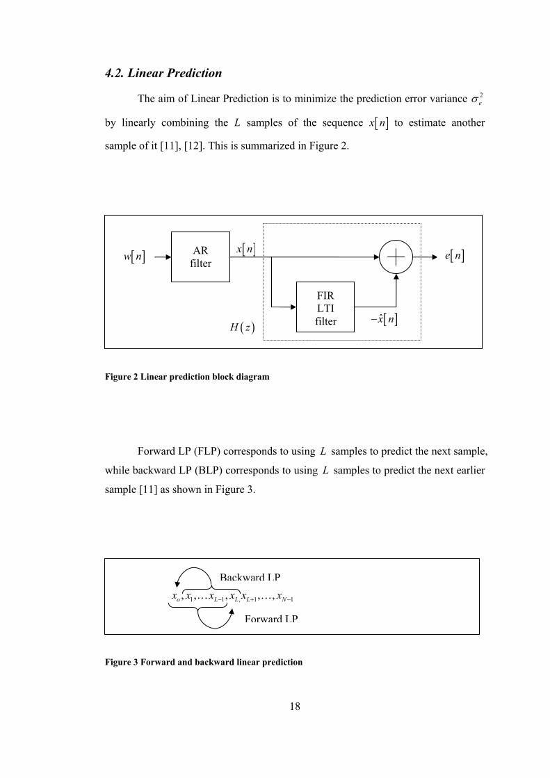
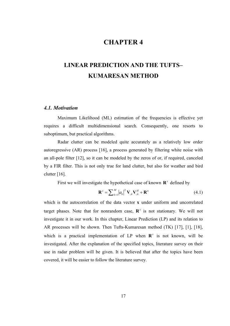
4.2. Linear Prediction
The aim of Linear Prediction is to minimize the prediction error variance 2eσ
by linearly combining the L samples of the sequence [ ]x n to estimate another
sample of it [11], [12]. This is summarized in Figure 2.
[ ]x n
Figure 2 Linear prediction block diagram
Forward LP (FLP) corresponds to using samples to predict the next sample,
while backward LP (BLP) corresponds to using samples to predict the next earlier
sample
L
L
[11] as shown in Figure 3.
Figure 3 Forward and backward linear prediction
AR filter
[ ]e n[ ]w n
FIR LTI filter [ ]x̂ n−
( )H z
1 1 , 1 1, , , , ,o L L L Nx x x x x x− + −… …Backward LP
Forward LP
18
The main equation for FLP is
[ ] [ ]*1
ˆ Lkk
x n g x n=
k= − −∑ (4.2)
where are the coefficients of the prediction-error filter (PEF)
shown in
*11, , , Lg … *g ( )H z
Figure 2. The coefficients can be found by satisfying the orthogonality
principle which states that [11]
[ ] [ ]{ }* 0, 1, ,E x n i e n i L− = = … . (4.3)
Using this principle the equations obtained, under the assumption that [ ]x n is Wide
Sense Stationary (WSS), are
( ) ( )*11 LIdeal Ideal k
kkH z z−
== +∑ g (4.4)
where
. (4.5) ( ) ( )(#
(1: ),(1: ) 1, 2: 1
TIdeal x xL L L+
⎡ ⎤= −⎢ ⎥⎣ ⎦g R R )
These equations are Ideal in the sense that perfect knowledge of xR is assumed. It
is well known that [11] if [ ]x n is an AR process generated by passing white noise
[ ]w n through the filter
( )
1
1 11 L k
kkD z b z−
=
=+∑
(4.6)
then
( )*Idealig ib= . (4.7)
In other words, as long as a linear predictor has order L larger than or equal to that
of the AR process, which is , P
0,Idealig L i P= ≥ > (4.8)
and ( ) ( )H z D z= (4.9)
as shown in Figure 4.
19
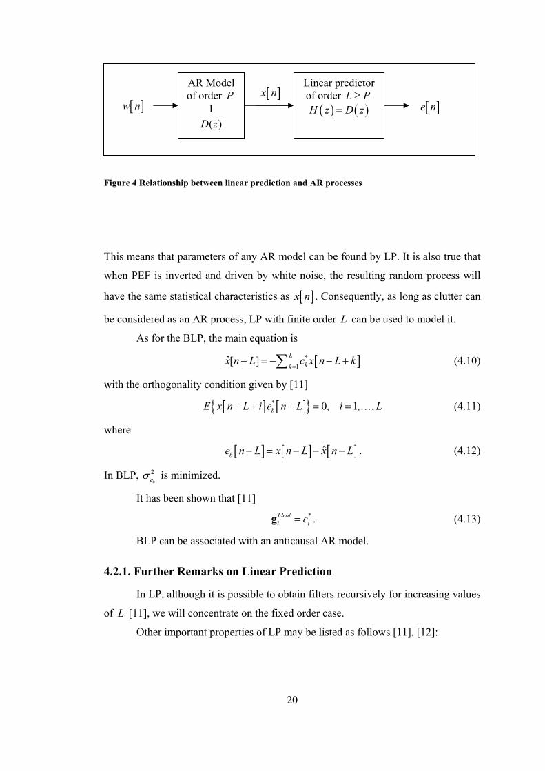
AR Model of order
Linear predictor of order [ ]x n P L P≥
[ ]w n [ ]e n ( ) ( )D z1( )D z
H z =
Figure 4 Relationship between linear prediction and AR processes
This means that parameters of any AR model can be found by LP. It is also true that
when PEF is inverted and driven by white noise, the resulting random process will
have the same statistical characteristics as [ ]x n . Consequently, as long as clutter can
be considered as an AR process, LP with finite order can be used to model it. L
As for the BLP, the main equation is
[ ]*1
ˆ[ ] Lkk
x n L c x n L k=
− = − − +∑ (4.10)
with the orthogonality condition given by [11]
[ ] [ ]{ }* 0, 1, ,bE x n L i e n L i L− + − = = … (4.11)
where
[ ] [ ] [ ]ˆbe n L x n L x n L− = − − − . (4.12)
In BLP, 2beσ is minimized.
It has been shown that [11]
*Ideali ci=g . (4.13)
BLP can be associated with an anticausal AR model.
4.2.1. Further Remarks on Linear Prediction
In LP, although it is possible to obtain filters recursively for increasing values
of L [11], we will concentrate on the fixed order case.
Other important properties of LP may be listed as follows [11], [12]:
20
1. If a fixed, but reasonably high order PEF is used, [ ]e n will have
approximately constant variance terms that are orthogonal to each other. This
means that [ ]e n is white noise. Thus PEF is a whitening filter.
2. For FLP, ( )H z is causal and minimum phase, which means that it is a causal
stable filter with a causal stable inverse. In other words, all of its zeros are
inside the unit circle.
3. For BLP, ( )H z is an anticausal and maximum phase polynomial.
4.3. Modified Tufts-Kumaresan Method
4.3.1. Overview of Tufts-Kumaresan Method
A practical way of implementing LP, when xR needs to be estimated from an
extremely limited number of observations is due to the methods developed by Tufts
and Kumaresan (TK) [17], [1], [18] for detecting complex exponentials in AWGN.
Tufts & Kumaresan’s method (TK method) brings performance improvement
to LP based frequency estimation methods at low by using the prior knowledge
about the rank
SNR
M of the signal correlation matrix. TK method estimates are
comparable to ML estimates and its performance is close to Cramér-Rao (CR) bound,
even when the data consists of closely spaced frequencies. Also, the value of at
which the accuracy of the frequency estimates departs drastically from the CR bound,
the threshold SN value, is brought much closer to that of ML by the use of TK
method.
SNR
R
Estimated correlation matrix is replaced by an estimated signal matrix in the
AWGN case. For the pulsed Doppler radar problem, the estimated correlation matrix
is replaced by an estimated signal and clutter correlation matrix, which is a necessary
modification to the TK method under scenarios containing clutter in addition to the
AWGN. This means filtering out some portion of the noise. Equivalently, the
forward-backward (FB) data matrix A can be approximated by a lower rank M
matrix where the FB data matrix is given by A
21
1 2 0
1 1
2 3* * *1 2* * *2 3 1
* * *1 1
L L
L L
N N N L
L
L
N L N L N
x x xx x x
x x xx x xx x x
x x x
− −
−
− − − −
+
− − + −
1
⎡ ⎤⎢ ⎥⎢ ⎥⎢ ⎥⎢ ⎥⎢ ⎥= ⎢ ⎥⎢ ⎥⎢ ⎥⎢ ⎥⎢ ⎥⎢ ⎥⎣ ⎦
A (4.14)
and tends to be full rank in the noisy case. Let be the reduced rank FB data matrix
corresponding to the actual FB data matrix A and be the reduced rank version of
the estimated correlation matrix
A
R
ˆ xR of the signal, clutter, and noise. The relations
between the specified matrices are as follows:
ˆ x H
H
=
=
R A A
R A A. (4.15)
This procedure is called principal components approximation [11], a method of
preserving signal subspace only.
4.3.2. Tufts-Kumaresan Algorithm Details
The TK algorithm has the following structure. Basically, the solution of
equation
= −Ag b (4.16)
is sought, where
(4.17) * * *1 1 0 1
T
L L N N Lx x x x x x+ − −⎡ ⎤= ⎣ ⎦b 1−
is the data vector and
[ ]1T
Lg g=g (4.18)
is the impulse response of the prediction filter of order . Equation L (4.16) is solved
for g in the least squares sense; i.e., one minimizes
2− −b Ag . (4.19)
The transfer function of the prediction-error filter ( )H z is given by
( ) 11 L k
kkH z g z−
== +∑ . (4.20)
22
For deterministic signals not corrupted by noise, the degree L of the
prediction-error filter polynomial ( )H z should satisfy [18]
round2MM L N
⎛ ⎞⎛ ⎞≤ ≤ −⎜ ⎜ ⎟⎜ ⎝ ⎠⎝ ⎠
⎟⎟ (4.21)
in order to have M zeros associated with signal and clutter when using the FBTK
method (TK method with the FB data matrix), where M equals M plus the number
of zeros required to model clutter. Besides L M− extraneous zeros, zeros at
positions
(4.22) 2 , 1, ,ij fe iπ = … M
are observed when used on a data consisting of undamped complex exponentials,
which is consistent with our signal model as explained in the next paragraph.
Targets can be modeled by complex exponentials and as can be seen from the
above explanation, TK is suitable in this aspect. Since clutter is an AR process, we
expect it to be modeled by one or more, M M− , complex exponentials just as the
targets. We have observed that if the radar antenna is not rotating, i.e., working
condition is zero , it is modeled by one complex exponential, and, increasing the
and/or CNR results in more poles being required in the AR model. Although a
table of number of poles needed to model the clutter can be obtained depending on
the operating conditions, it is not necessary as we will explain in Chapter 7. An
algorithm will be developed to decide on
rpm
rpm
M and then the targets will be identified
based on clutter regions. Under these circumstances, TK is suitable in radar signal
modeling as a whole, since it is one of the most successful high resolution frequency
estimation techniques.
For the FTK or BTK methods, the condition becomes [18]
( )M L N M≤ ≤ − (4.23)
and one uses the upper or the lower half of the matrix in the calculations, thus the
name FTK or BTK, respectively.
A
If the prediction filter coefficients are selected to have minimum Euclidean
norm and the first coefficient is taken to be unity, the L M− extraneous zeros of the
23
filter polynomial are approximately uniformly distributed inside the unit circle [18],
[11]. To observe this fact, one can factor ( )H z as
( ) ( ) ( )2H z H z= 1H z (4.24)
where has ( )1H z M
( )z
zeros modeling the signal and the clutter; and has
zeros, which are the extraneous zeros. The polynomial can be
associated with a prediction-error filter operating on the data-sequence defined by the
coefficients of and yielding the error sequence, which are the coefficients of
. Minimizing the Euclidean norm of
( )2H z
( )zL M−
(H z
2H
1H
) ( )H z , while keeping its first coefficient
at unity in order to prevent a zero solution, is identical to minimizing the error energy
in the autocorrelation method of linear prediction. It is a known fact that the
prediction-error filter is minimum phase [11] and its zeros have magnitude less than
unity, thus proving that extraneous zeros of L M− ( )H z fall in the unit circle.
The above observation is necessary to identify the two groups of zeros: those
related to signal and clutter, and the extraneous or spurious zeros. By using the
Moore-Penrose pseudoinverse [19] of A in calculating g , we satisfy the minimum
Euclidean norm condition on g .
However, when the data is noisy, the extraneous zeros can lie closer to or
outside the unit circle. Rank reduction alleviates this problem by effective SN
enhancement. The best lower rank of
R
M approximation (in term of Frobenius norm)
to a given matrix can be found based on Singular Value Decomposition (SVD), by
setting all but M of its largest singular values to zero [17], [1].
The solution to equation (4.16), satisfying the two constraints, is
( )#≈ = −g g A b (4.25)
where is the reduced rank pseudoinverse of A . To find an explicit form of
equation
#A
(4.25), we start by finding the SVD of A
( )HA AS V A=A U (4.26)
where the columns of are eigenvectors of AU HAA , the columns of are
eigenvectors of , and the singular values on the diagonal of are the square
AVHA A AS
24
roots of the nonzero eigenvalues of both HAA
#A
and . Once the SVD of A is
obtained, its Moore-Penrose pseudoinverse is given by where
is obtained from by replacing each nonzero diagonal entry by its reciprocal.
Using only
HA A
( ) ( )TA A AIV S U
H
AIS AS
M singular values instead of the matrix to achieve rank reduction, AIS g
in equation (4.25) is obtained as
( ) :,
1
H
S:,
A AiV
,
M iAii i
=≈ = −∑
U bg g . (4.27)
g does not minimize the prediction-error energy, but is an approximation of
the noiseless situation.
Lastly, the angle (in radians) between each of the M zeros of closest
to the unit circle and the positive real axis in the complex plane when divided by
( )H z
2π
gives the frequency estimates. The target frequency estimates if ’s are found after
eliminating M M−
( )H z
of the obtained frequency estimates that model the clutter and
thus fall in one of the clutter regions to be defined. A pictorial representation of the
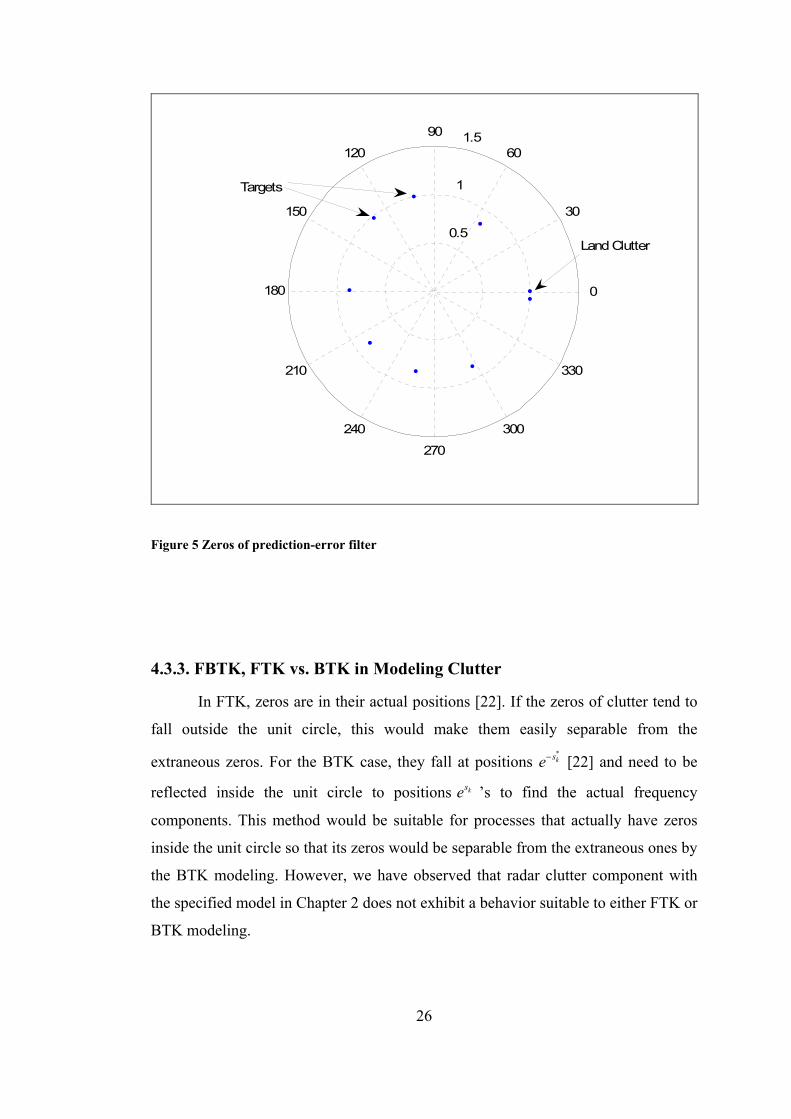
zeros of is given in Figure 5 where 9,L M 2 and 4M= = = .
TK method modified with truncation control, i.e., rank reduction to values
other than M , selecting more zeros closer to the unit circle than a threshold and
eliminating them from their magnitude is investigated in [20], [21].
25
0.5
1
1.5
30
210
60
240
90
270
120
300
150
330
180 0
Land Clutter
Targets
Figure 5 Zeros of prediction-error filter
4.3.3. FBTK, FTK vs. BTK in Modeling Clutter
In FTK, zeros are in their actual positions [22]. If the zeros of clutter tend to
fall outside the unit circle, this would make them easily separable from the
extraneous zeros. For the BTK case, they fall at positions *kse− [22] and need to be
reflected inside the unit circle to positions kse ’s to find the actual frequency
components. This method would be suitable for processes that actually have zeros
inside the unit circle so that its zeros would be separable from the extraneous ones by
the BTK modeling. However, we have observed that radar clutter component with
the specified model in Chapter 2 does not exhibit a behavior suitable to either FTK or
BTK modeling.
26
4.3.4. FBTK Noise Reduced Data Vector Version
We have devised a version of FBTK by also reducing the effect of noise in
the data vector (4.17). We form the concatenation of the data matrix and the data
vector as
[ ]b A (4.28)
and retaining M of the singular values of this matrix, re-obtain the noise reduced
versions of b and from the corresponding positions of the same size, but rank
reduced concatenated matrix. All the other steps are the same with the FBTK
algorithm after this step. The performance and necessity of this modification are
discussed during the simulations under the algorithm name ‘FBTK, NRDV,’ where
NRDV stands for noise reduced data vector.
A
4.4. Distinguishing Clutter and Targets: the Concept of Clutter Region
In works found in the literature, land clutter is distinguished from its velocity
being nearest to zero [5]. However, we cannot distinguish it from the large power of
its singular value, since depending on CNR this condition may not be true. For a
given set of radar parameters, we performed simulations to specify clutter regions,
one for each source of clutter. If a frequency estimate falls in a clutter region, it is
identified as a clutter component resulting in separation of the frequencies of targets
and clutter.
With this technique, clutter spread observed in its power spectrum is not
always modeled by a single DC term, but it can be modeled by more than one
prediction-error filter zeros falling in the clutter region near location at zero
frequency with a certain width, i.e., land clutter region, or around any other
frequency with the same width for moving clutter case. Further explanation will be
provided in Chapter 7.
4.5. Linear Predictor as a Radar Processor
When using LP in a radar detector a filter bank is unnecessary, since the
processor is not designed based on specific target frequencies. In other words, a
single LP processor is sufficient. It can be designed as a linear prediction-error filter
by using the a priori knowledge on clutter. When there is a target its output is
27
expected to consist of a target component plus suppressed clutter. However, we point
out that although LP can be used to filter the radar echo in order to get rid of clutter
followed by target detection, it is also possible and requires less computation to
include both the targets and the clutter, possibly both land and moving weather
clutter, in its design. In this way we can achieve clutter filtering (including weather
clutter), multiple target detection and high resolution velocity estimation with a
single processor. Also using LP in a way to estimate other samples than the next or
the previous sample is studied [8].
LP in slow time samples can be used as an efficient tool to estimate Doppler
frequencies, in addition to some other methods, but not in its FB version and for
mean Doppler frequency estimation of weather radar signal in the presence of single
clutter source which is the ground clutter in [5] with L fixed at 2 and the estimated
frequency further from zero corresponding to weather clutter and that near zero
frequency corresponding to ground clutter. In this work the frequency range not
affected by clutter is reported to be [ ]0.2,0.8 with RMSE ≤ 0.04. After separating the
target and the clutter, LP is used to c utter in ancel cl
ilter can be seen to have some
similar
[23]. It is used to model both the
ship echo and Bragg lines in [24]. The Bragg lines are the scattering from surface
waves which have wavelength equal to one half of the radar wavelength and move
directly away or towards the receiving radar. A sea clutter whitening preprocessing is
also developed based on multiple bursts in [24].
Our approach of using LP as a clutter f
ities with [24]. However, there are major differences such as Coherent
Integration Time’s (CIT) required. For the given work, under favorable conditions
CITs of 2s. are reported for ships and under normal conditions for aircrafts, whereas
our observation time for a typical 10PRF KHz= is in the order of ms. One reason
for this difference may be the fact th the similar processor to a different
scenario where Bragg scattering of the ocean surface is not the major source of
clutter. Continuing with the differences observed in our work, our radar is a land
based one with multiple clutter sources due to weather clutter and can perform target
discrimination. We analyzed its performance depending on the various parameters
used and compared with other high resolution spectrum estimation algorithms. We
also use a different method to find the number of frequencies, which is explained in
at we applied
28

29
Chapter 7, since Akaike Information Criterion (AIC) [25] used in [24] is not a
suitable method for short data lengths [12] and non-Gaussian data, which is the case
for our observations under the assumption of random target phases. We intentionally
did not assume a distribution for the target magnitude in order to be able to
generalize results to arbitrary distributions after obtaining results at different
amplitude values of complex multipliers.
CHAPTER 5
OTHER HIGH RESOLUTION LINE SPECTRA
ESTIMATION TECHNIQUES
In this chapter DTFT, MUSIC and ESPRIT algorithms as applied to target
detection in radar clutter will be studied. A literature survey on the use of MUSIC in
radar problem will be provided after the descriptions of the algorithm. Lastly, it will
be made clear why ML algorithm requires the output of one of the defined high
resolution frequency estimation algorithms in order to function properly.
5.1. Can Pure DFT Be an Alternative?
The DTFT of a sample vector x defined in equation (2.5) (obtained by zero-
padded DFT) is shown in Figure 6. Although two targets at frequencies
[ ] [ ]1 2 0.2813 0.3563f f = under strong clutter are present, even the presence of
two targets cannot be detected As a result, one can conclude that without clutter
suppression or pre-whitening a promising result cannot be obtained with Fourier
Transformation approach to frequency estimation. We have also observed, as
explained in section 3.1., that MAXSIR or MTI type methods that suppress clutter do
not provide the required resolution to differentiate two targets.
Although, when noise is not present, three samples are enough to distinguish
a complex exponential from another including phase and magnitude, especially if the
samples do not cover an integer number of periods of the Doppler tone from a target
in a pulsed Doppler radar (periodic extension of this waveform determines the signal
being processed [26]), DFT suffers from the sidelobes of complex exponentials
burying nearby complex exponential peaks. In other words, spectral lines widen in
frequency domain [3]. In this case larger DFT lengths with zero-padding do not help.
With DFT, frequency resolution is inversely proportional to the number of data
30
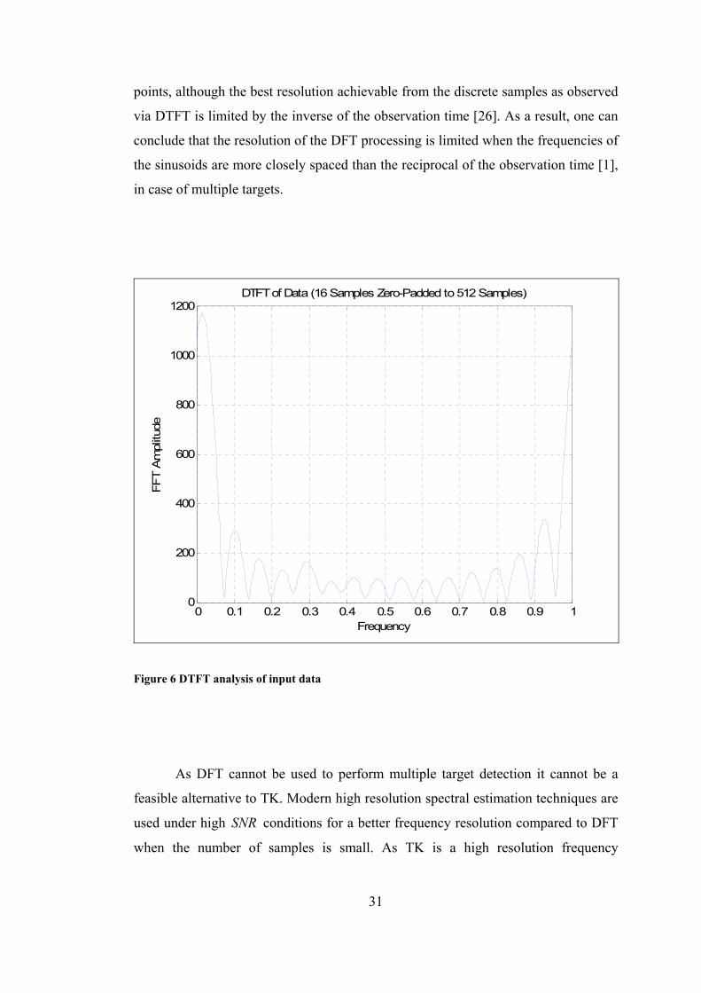
points, although the best resolution achievable from the discrete samples as observed
via DTFT is limited by the inverse of the observation time [26]. As a result, one can
conclude that the resolution of the DFT processing is limited when the frequencies of
the sinusoids are more closely spaced than the reciprocal of the observation time [1],
in case of multiple targets.
0 0.1 0.2 0.3 0.4 0.5 0.6 0.7 0.8 0.9 10
200
400
600
800
1000
1200
FFT
Am
plitu
de
DTFT of Data (16 Samples Zero-Padded to 512 Samples)
Frequency
Figure 6 DTFT analysis of input data
As DFT cannot be used to perform multiple target detection it cannot be a
feasible alternative to TK. Modern high resolution spectral estimation techniques are
used under high conditions for a better frequency resolution compared to DFT
when the number of samples is small. As TK is a high resolution frequency
SNR
31
estimation technique suitable for signals possessing line components like target
echoes, other well known algorithms such as MUSIC [12], [11] and ESPRIT [11]
with their various suggested versions that we will review are also applicable. These
algorithms are not originally developed for radar scenarios under clutter, but they are
basically designed for data corrupted in AWGN. To use them for modeling clutter,
we will make the necessary modifications as we did for TK and analyze their
performance in comparison with TK’s. One can say that line component estimation
techniques are not suitable for an arbitrary clutter plus noise covariance matrix. Only
when clutter can be modeled as a group of targets, the above mentioned algorithms
are suitable.
5.2. MUSIC Algorithm
In this section original MUSIC algorithm will be explained followed by its
implementation under single snapshot observation and the necessary modifications
needed in order to apply it to our problem of detection multiple targets under radar
clutter. The last sub-section will also detail various versions of the MUSIC algorithm
applied to our problem.
5.2.1. Basic MUSIC Algorithm
In this sub-section the observation x will be assumed to be free of clutter to
explain the basic version of the MUSIC algorithm. If the eigenvalues of the actual
correlation matrix of the data x containing M complex exponentials of unknown
amplitude, phase, and frequency, xR , are arranged in decreasing order, largest M of
them will correspond to signal subspace with the rest belonging to the noise subspace
[12], [11]. For a Hermitian matrix xR , its eigenvectors will be orthogonal resulting
in the above defined subspaces to be orthogonal [12]. Thus, one over the magnitude
square of DTFT of the noise subspace eigenvectors will have peaks at the
frequencies of the complex exponential signals present in x . Equivalently, noise
subspace eigenfilters formed by the z-Transformation of the eigenvectors
corresponding to the noise will have M of its roots lying on the unit circle at the
frequencies of the complex exponential signals [12]. The frequency estimates can be
obtained from the angles of these roots. However, other zeros of this polynomial can
32
also be located near the unit circle making it hard to distinguish them from signal
zeros. Also, when an estimate of xR , ˆ xR , is used, signal zeros may not remain on
the unit circle. These effects are reduced and spurious roots are moved away from the
unit circle by means of averaging used in the algorithm called MUltiple SIgnal
Classification (MUSIC).
Let denote the noise subspace eigenvectors of an
estimated autocorrelation matrix
:, , 1,xk k M= +E …, L
ˆ xR of the data with size L . These are
distinguished from signal subspace eigenvectors by having the smallest L M
L×
−
eigenvalues. One then forms the polynomial
( ) ( ) ( )( )**1l M= +
kl k z− −=
1l lD z E z E z=
,+
L∑
:,1
L xk=
(5.1)
where
( ) ( )1 , 1,E z l M L=∑ E … . (5.2)
The last step is to choose 2M roots of the polynomial in equation (5.1) that are
closest to the unit circle and, eliminating double roots, select M of them whose
angles (in radians) will provide the frequency estimates.
We have focused on the root-MUSIC algorithm since otherwise there is the
task of peak detection to find the signal frequencies from one over equation (5.2)
evaluated at 2j fz e π= .
Note that TK and MUSIC involve nonlinear operations and their performance
analysis is not simple, so simulation will be used as a tool to evaluate the
performances.
5.2.2. Estimation of the Autocorrelation Matrix from Single Snapshot
Observation
Usually ˆ xR is estimated from multiple observations. The use of MUSIC
technique under cases involving single snapshot is justified in [27].
The main rationale behind estimating the autocorrelation matrix of the
observation from a single burst of observation is to partition the data into pieces to
create more virtual instances of the observation instead of directly using Hxx as the
33
estimated autocorrelation matrix. The partitioning of the data can be done in one
direction or in both directions as will be explained next.
Defining
1 0
1
1
L
covN L L
N N L
x x
x x
x x
−
−
− −
−
⎡ ⎤⎢ ⎥⎢ ⎥⎢ ⎥=⎢ ⎥⎢ ⎥⎢ ⎥⎣ ⎦
X , (5.3)
one can form the expression for a possible estimate of the autocorrelation matrix of
the observation as
( )ˆ Hx,cov cov covX X=R . (5.4)
For this autocorrelation matrix estimate, partitions of the data are formed in a single
direction. MUSIC algorithm resulting from such an autocorrelation estimate will be
called simply MUSIC algorithm, in contrast to the ‘MUSIC, FB’ resulting from
using
1 0
1
1*0 1
**1
* *1
L
N L L
Nmod
L
N LL
N L N
*N L
x x
x x
x xx x
xx
x x
−
− −
−
−
−−
− −
−
⎡ ⎤⎢ ⎥⎢ ⎥⎢ ⎥⎢ ⎥⎢ ⎥⎢ ⎥⎢ ⎥=⎢ ⎥⎢ ⎥⎢ ⎥⎢ ⎥⎢ ⎥⎢ ⎥⎢ ⎥⎣ ⎦
X (5.5)
to estimate the autocorrelation matrix of the observation as
( ) ( ),ˆ Hx mod mod mod=R X X (5.6)
where pieces of the data are used in both directions to obtained the autocorrelation
matrix estimate.
34
5.2.3. MUSIC Algorithm as Applied to Our Problem
For the basic MUSIC algorithm explained in sub-section 5.2.1, there was no
clutter, hence no clutter region, but only AWGN.
We perform the eigendecomposition of ˆ xR (either ,ˆ x covR , ,ˆ x modR ). If ,ˆ x modR
is used there will be the letters ‘FB’ in naming of the algorithms. Two cases will be
investigated: performing whitening with the matrix when it is known, or, omitting
this step. The first case is further classified into two: Clutter can be counted as targets
after whitening or only target frequencies can be sought.
nR
First let us explain the whitened version of MUSIC [28], [11]: We define the
generalized eigenvalue problem to be satisfied by the noise subspace (if clutter still
needs to be associated with target subspace after whitening it will be named as ‘M,
W (Clutter Counted as Target)’ or ‘M, WFB (Clutter Counted as Target)’ otherwise
just ‘M, W’ or ‘M, WFB’):
:, :,ˆ x x x n
k kλ=R E R Exk . (5.7)
Here :,xkE is orthogonal to signal subspace and our aim is to find these vectors. A
method to accomplish this task is by performing Cholesky decomposition of as nR
. (5.8) n H=R C C
Next one performs the operation ,ˆ x whitened H x 1ˆ− −=R C R C . (5.9)
The eigendecomposition of equation (5.9) is given by
, , , ,ˆ x whitened x whitened x whitened x whitened=R V V D (5.10)
where ,x whitenedV has the eigenvectors of ,ˆ x whitenedR as its columns and ,x whitenedD is a
diagonal matrix of eigenvalues. Comparing equation (5.11), which is written by
inserting equation (5.9) into equation (5.10) and multiplying both sides by HC form
right,
1 , 1 , ,ˆ x x whitened n x whitened x whitened− −=R C V R C V D (5.11)
with equation (5.7), one can obtain
1 ,:, :,x x whitenedk k
−=E C V (5.12)
and form the polynomial
,+ . (5.13) ( ) ( )11 ,,1
, 1,L kx whitenedl k lk
E z z l M L− −−=
= =∑ C V …
35
M M=
otherw
If is used, we have the ‘(Clutter Counted as Targ
algorith
et)’ version of the
m, ise M M= is used after whitening.
As a final step, one forms and chooses 2M roots of the polynomial
( ) ( ) ( )( )*11L
l ll MD z E z z= +
= ∑ *
E (5.14)
at are closest to the unit circle and, eliminating doubleth roots, selects M of them
whose angles (in radians) will provide the frequency estimates. For the ‘(Clutter
Counted as Target)’ case we have the clutter region concept, otherwise this concept
is not used after whitening. For all M groupings of 2M frequency estimates, we
have calculated the minimum of the distances between all possible two pairs of M
frequency estimates in mod 1. We have selected M of the roots such that they ha
the maximum of the calculated minimum distance. As a result, we eliminate
frequencies that are originating from the same frequency and do not count them
twice.
ve
Non-whitened MUSIC uses the same algorithm as above, with the only
change that in equation nR
d
(5.8) is taken as I having the same size assuming clutter
as targets an M M= . An instance of the MUSIC spectrum for the non-whitened
case for two targets at frequencies [ ] [ ]1 2 0.2813 0.3563f f = is given in Figure 7,
which is obtained by evaluating o 4)ne ove e equation (5.1r th at 2j fz e π= . The
presence of two peaks near the target frequencies reveals the resolution capability of
MUSIC and its applicability to our problem.
36
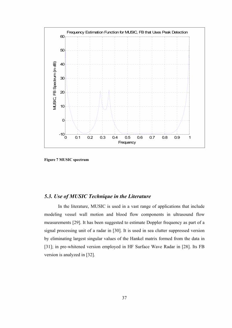
0 0.1 0.2 0.3 0.4 0.5 0.6 0.7 0.8 0.9 1-10
0
10
20
30
40
50
60
Frequency
MU
SIC
, FB
Spe
ctru
m (i
n dB
)
Frequency Estimation Function for MUSIC, FB that Uses Peak Detection
Figure 7 MUSIC spectrum
5.3. Use of MUSIC Technique in the Literature
In the literature, MUSIC is used in a vast range of applications that include
modeling vessel wall motion and blood flow components in ultrasound flow
measurements [29]. It has been suggested to estimate Doppler frequency as part of a
signal processing unit of a radar in [30]. It is used in sea clutter suppressed version
by eliminating largest singular values of the Hankel matrix formed from the data in
[31]; in pre-whitened version employed in HF Surface Wave Radar in [28]. Its FB
version is analyzed in [32].
37
5.4. Total Least Squares ESPRIT Algorithm
5.4.1. Basic Total Least Squares ESPRIT Algorithm
The essence of the basic ESPRIT algorithm [11] will be explained in this sub-
section.
Firstly, one obtains the M signal subspace eigenvectors of ˆ xR and forms the
matrix by placing them as the columns. Assume there is a hypothetical matrix V
having the sought complex exponential signals placed at its columns. Since the
columns of matrices B and span the same subspace, a nonsingular transformation
can be defined between them:
B
V
=B Vϒ . (5.15)
One can observe that due to the special nature of matix , V
(5.16) ( ) ( )2: ,: 1: 1 ,:end end−=V V Φ
can be written where is a diagonal matrix with entries: Φ
,kj
k k e ω=Φ . (5.17)
Using equation (5.16) in equation (5.15), the following equations can be obtained
(5.18) ( ) ( )
( ) ( )
1: 1 ,: 1: 1 ,:
2: ,: 1: 1 ,:
end end
end end
−
−
=
=
B V
B V Φ
ϒ
ϒ
−
)
that can be combined to get
( ) (1: 1 ,: 2: ,:end end− =B Ψ B (5.19)
where
1−=Ψ Φϒ ϒ . (5.20)
Equation (5.19) can be solved in total least squares sense [11] to obtain Ψ . The
angles of the eigenvectors of Ψ will yield the signal frequency estimates as can be
seen from equations (5.20) and (5.17).
5.4.2. Total Least Squares ESPRIT Algorithm as Applied to Our Problem
Similar to the MUSIC algorithm, two versions of the Estimation of Signal
Parameters via Rotational Invariance Techniques (ESPRIT) algorithm [11] will be
investigated: One that employs pre-whitening with its two versions and the other one
38
that treats clutter components as targets and assumes operation under AWGN.
Autocorrelation matrix of the data vector can be estimated in two different ways as
pointed out in MUSIC algorithm, resulting in ESPRIT or ‘ESPRIT, FB’. There is no
difference between these two versions except the mentioned step.
Let us now explain the algorithm. First we need to obtain the eigenvectors of
ˆ xRnR
corresponding to non-noise subspace. Similar to MUSIC algorithm, when matrix
is used in the calculations instead of the matrix I , clutter can be counted still in
the signal subspace, ‘(Clutter Counted as Target)’ version that requires clutter region
definition, or can be included in the noise subspace with no need for clutter region.
We define the whitening transformation
( )1
2n−
=y R x . (5.21)
One needs the signal subspace eigenvectors and eigenvalues in the whitened domain
in order to obtain the corresponding eigenvectors of ˆ xR . Defining { }ˆ y HE=R yy ,
(5.22) ˆ y y y y=R V V D
is the equation satisfied in whitened interference domain. Multiplying both sides of
equation (5.22) from the left by ( )1
2nR after inserting ( ) ( )1 1
2 2ˆ ˆy n nx
− −
=R R R R in
equation (5.22), one obtains
( ) ( ),
1: , 1:ˆ , ,x g x n g x g x
L L=R V R V D (5.23)
where
( )1
2,
,
g x n y
g x y
−
=
=
V R
D D
V . (5.24)
As a result, eigenvectors of ˆ xR related to the target, and possibly, clutter subspace
are
( ) ( ) ( ),
1: , 1: :, 1:n g
L LxM
=B R V . (5.25)
Here M can be M or M , similar to the case in MUSIC method, depending on the
algorithm. Since the columns of B and span the same subspace V
=B Vϒ (5.26)
39
can be written, where V is a hypothetical matrix that contains target, and possibly
clutter echoes depending on the version of the algorithm, expressed in complex
exponentials and placed at the columns of this matrix.
Lastly, one finds the TLS solution of equation (5.19) which is given as [11]
( ) ( ) ( )1: 1 ,: 2: ,:
HB B Bend end−
⎡ ⎤ =⎣ ⎦B B U S V (5.27)
( ) ( ) ( ) ( )( ) 1
1: , 1: 1: , 1:B B
M M end M end M end
−
+ + += −Ψ V V . (5.28)
The frequency estimates are then obtained as
( )HΨ Ψ Ψ=Ψ V D V (5.29)
. (5.30) , , 1, ,k k k kω Ψ= ∠ =D … M
Note that although we have taken into account the non-white autocorrelation
of clutter plus noise, it will be seen in section 9.2. that as in the case of MUSIC it
gives more reliable results to run the algorithm for M , rather than for M and then
use frequency elimination based on clutter region for obtaining target frequencies.
Another alternative way of implementing ESPRIT can be based on assuming
as matrix I and doing the same derivations. One then obtains total number of nR
M target and clutter frequencies by selecting M M= .
5.5. High Resolution Methods Combined with ML
Estimates obtained from high resolution line component estimations
techniques can be improved in an optimal sense. Since the likelihood function
possesses lots of valleys, one needs a good initial guess of the optimal point for
convergence to the global optimum if not using a difficult multidimensional search.
Otherwise, the ML algorithm will stuck to a local optimum point. The aim of the TK,
MUSIC or ESPRIT can be to form the aforementioned initial point [11], if further
reduction of variance and unbiasedness is desired.
Log-Likelihood function (defined in equation (3.6)) as a function of 1f and
2f is plotted in Figure 8 by finding the optimal complex coefficients for each
frequency using equation (3.17) under the presence of two targets having frequencies
[ ] [ ]1 2 0.2813 0.3563f f = . Likelihood function, whose minimum is sought, has
40
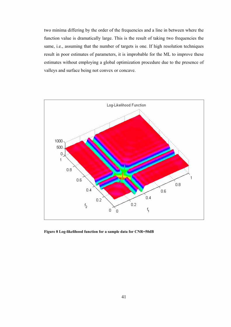
two minima differing by the order of the frequencies and a line in between where the
function value is dramatically large. This is the result of taking two frequencies the
same, i.e., assuming that the number of targets is one. If high resolution techniques
result in poor estimates of parameters, it is improbable for the ML to improve these
estimates without employing a global optimization procedure due to the presence of
valleys and surface being not convex or concave.
Figure 8 Log-likelihood function for a sample data for CNR=50dB
41
CHAPTER 6
DETERMINATION OF AMPLITUDES AND PHASES
Finding complex amplitudes after the frequency estimates are obtained can be
realized via two different techniques: Least Squares Estimation or Maximum
Likelihood technique. Their application to radar observations corrupted with clutter
will be explained in this chapter followed by a brief comparison of high resolution
line spectra estimation algorithms.
6.1. Least Squares Estimator
This method uses the fact that radar clutter can be modeled as a sum of
complex exponentials. Obtaining frequency estimates, one can form the matrix
with entries
F
[10]
( )( ), exp 1 , 1, , , 1, ,k p pj k k N pω= − = =F … … M (6.1)
as an intermediate step for obtaining the amplitudes and phases as follows:
( ) 1
1T H H
Ma a−
=⎡ ⎤⎣ ⎦ F F F x . (6.2)
Note that we have obtained M complex coefficients although only M of
them are associated with targets as seen in equation (2.5). Using the fact that clutter
is contained in a clutter region with a known mean (D.C. frequency for land clutter),
one can distinguish the M complex exponentials of the targets. If the version of the
high resolution frequency estimation algorithm yields only target frequencies, a
complex exponential signal with a frequency of zero should be associated with land
clutter and M in equations (6.1) and (6.2) should be selected as 1M + .
In cases where clutter is modeled with complex exponentials differing very
little in frequency, inverse operation in (6.2) can be replaced by pseudoinverse.
42
6.2. Maximum Likelihood Derivative Equations
Here, we make the assumption that is known and after frequencies of the
targets have been determined use equations
nR
(3.9), which are repeated here for
convenience,
43
M :, :, :,10, 1, ,MH H
k k l lla k
=− + = =∑V Qx V Q V … (6.3)
to find the amplitudes and phases of the targets.
6.3. Comparison of Techniques
Methods can be classified based on the use of noise autocorrelation matrix: It
can be the actual one or the estimated one. ML, whitened versions of MUSIC,
HWMAXSIR, and versions of ESPRIT that require are somewhat ideal in the
sense that actual version of this matrix is supplied to the algorithms although there
would be estimation errors in practice. Other algorithms do not require this matrix. If
one uses ML derivative equations to obtain complex coefficients in the model, it is
again assumed that actual is known. On the other hand, the least squares
estimator does not use .
nR
nRnR
Computational complexity of the algorithms can be accessed by comparing
the required operations detailed in the explanation of the algorithms and the time the
desired processor spends to perform these tasks. A careful study of this issue has not
been performed yet.
CHAPTER 7
CLUTTER REGIONS AND DETERMINATION OF THE
NUMBER OF SIGNAL PLUS CLUTTER ZEROS
The number of complex exponentials that comprise targets and the clutter can
be determined by various methods: observing the sharp fall in the magnitudes of the
eigenvalues of the estimated autocorrelation matrix of observation, ˆ xR , or in the
magnitudes of the singular values of matrix A defined in equation (4.14) [1], which
fails when the frequencies to be estimated are close to each other; using CFAR
hypothesis tests employing multiple thresholds on the noise subspace energy found
by the sum of squares of the corresponding singular values [33]; applying Akaike
Information Criterion (AIC), Minimum Description Length (MDL) criterion [25] etc.
It is also possible that the number of targets M is provided by another block
of the system and one focuses on the high precision velocity estimation of the targets
that are in the same folded range. For this case, M M− can be changed depending
on and which dictate clutter spreading, or it can be chosen as the
maximum value under the specified operational conditions. We have observed that at
zero rpm , the clutter is modeled just like a single target for all CNR . However, as
increases for different CNR levels, clutter can be thought of as a group of
targets having similar Doppler frequencies. On the other hand, targets at all rpm ’s
and ’s are modeled by one zero. When the largest possible
CNR
SNR
rpm
rpm
M M− value is
chosen, this covers possible lower values since the estimates beyond the actual
number of signal plus clutter estimates will have very small magnitudes. In this
method, with the assumption that number of signals, equivalently the number of
targets in the same folded range, is provided, zeros falling in the clutter region are
eliminated and if the remaining number of zeros is larger than the number of signal
44
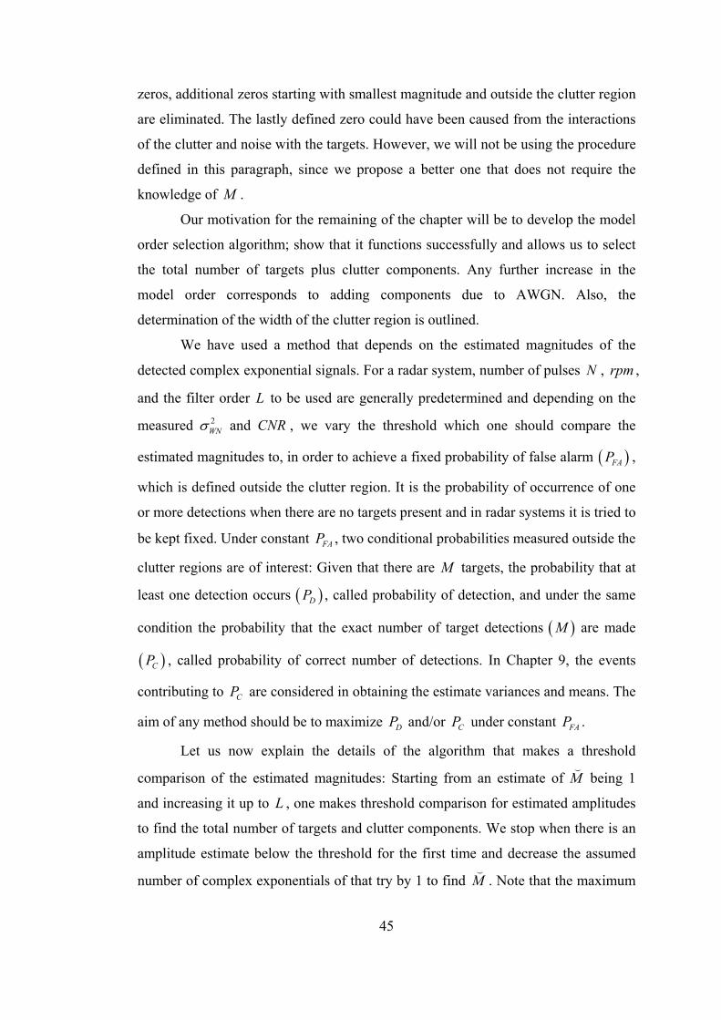
zeros, additional zeros starting with smallest magnitude and outside the clutter region
are eliminated. The lastly defined zero could have been caused from the interactions
of the clutter and noise with the targets. However, we will not be using the procedure
defined in this paragraph, since we propose a better one that does not require the
knowledge of M .
Our motivation for the remaining of the chapter will be to develop the model
order selection algorithm; show that it functions successfully and allows us to select
the total number of targets plus clutter components. Any further increase in the
model order corresponds to adding components due to AWGN. Also, the
determination of the width of the clutter region is outlined.
We have used a method that depends on the estimated magnitudes of the
detected complex exponential signals. For a radar system, number of pulses , ,
and the filter order L to be used are generally predetermined and depending on the
measured
N rpm
2WNσ and , we vary the threshold which one should compare the
estimated magnitudes to, in order to achieve a fixed probability of false alarm
CNR
( )FAP ,
which is defined outside the clutter region. It is the probability of occurrence of one
or more detections when there are no targets present and in radar systems it is tried to
be kept fixed. Under constant , two conditional probabilities measured outside the
clutter regions are of interest: Given that there are
FAP
M targets, the probability that at
least one detection occurs ( )DP , called probability of detection, and under the same
condition the probability that the exact number of target detections ( )M are made
, called probability of correct number of detections. In Chapter 9, the events
contributing to are considered in obtaining the estimate variances and means. The
aim of any method should be to maximize
( CP )
CP
DP and/or under constant . CP FAP
Let us now explain the details of the algorithm that makes a threshold
comparison of the estimated magnitudes: Starting from an estimate of M being 1
and increasing it up to , one makes threshold comparison for estimated amplitudes
to find the total number of targets and clutter components. We stop when there is an
amplitude estimate below the threshold for the first time and decrease the assumed
number of complex exponentials of that try by 1 to find
L
M . Note that the maximum
45
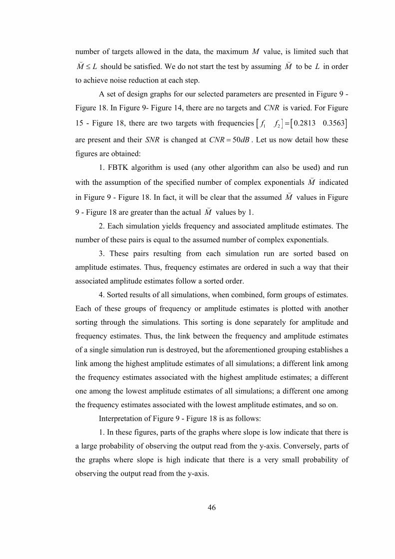
number of targets allowed in the data, the maximum M value, is limited such that
M L≤ should be satisfied. We do not start the test by assuming M to be in order
to achieve noise reduction at each step.
L
A set of design graphs for our selected parameters are presented in Figure 9 -
Figure 18. In Figure 9- Figure 14, there are no targets and CN is varied. For R Figure
15 - Figure 18, there are two targets with frequencies [ ] [ ]1 2f f 0.2813 0.3563=
are present and their SNR is changed at 50CNR dB= . Let us now detail how these
figures are obtained:
1. FBTK algorithm is used (any other algorithm can also be used) and run
with the assumption of the specified number of complex exponentials M indicated
in Figure 9 - Figure 18. In fact, it will be clear that the assumed M values in Figure
9 - Figure 18 are greater than the actual M values by 1.
2. Each simulation yields frequency and associated amplitude estimates. The
number of these pairs is equal to the assumed number of complex exponentials.
3. These pairs resulting from each simulation run are sorted based on
amplitude estimates. Thus, frequency estimates are ordered in such a way that their
associated amplitude estimates follow a sorted order.
4. Sorted results of all simulations, when combined, form groups of estimates.
Each of these groups of frequency or amplitude estimates is plotted with another
sorting through the simulations. This sorting is done separately for amplitude and
frequency estimates. Thus, the link between the frequency and amplitude estimates
of a single simulation run is destroyed, but the aforementioned grouping establishes a
link among the highest amplitude estimates of all simulations; a different link among
the frequency estimates associated with the highest amplitude estimates; a different
one among the lowest amplitude estimates of all simulations; a different one among
the frequency estimates associated with the lowest amplitude estimates, and so on.
Interpretation of Figure 9 - Figure 18 is as follows:
1. In these figures, parts of the graphs where slope is low indicate that there is
a large probability of observing the output read from the y-axis. Conversely, parts of
the graphs where slope is high indicate that there is a very small probability of
observing the output read from the y-axis.
46
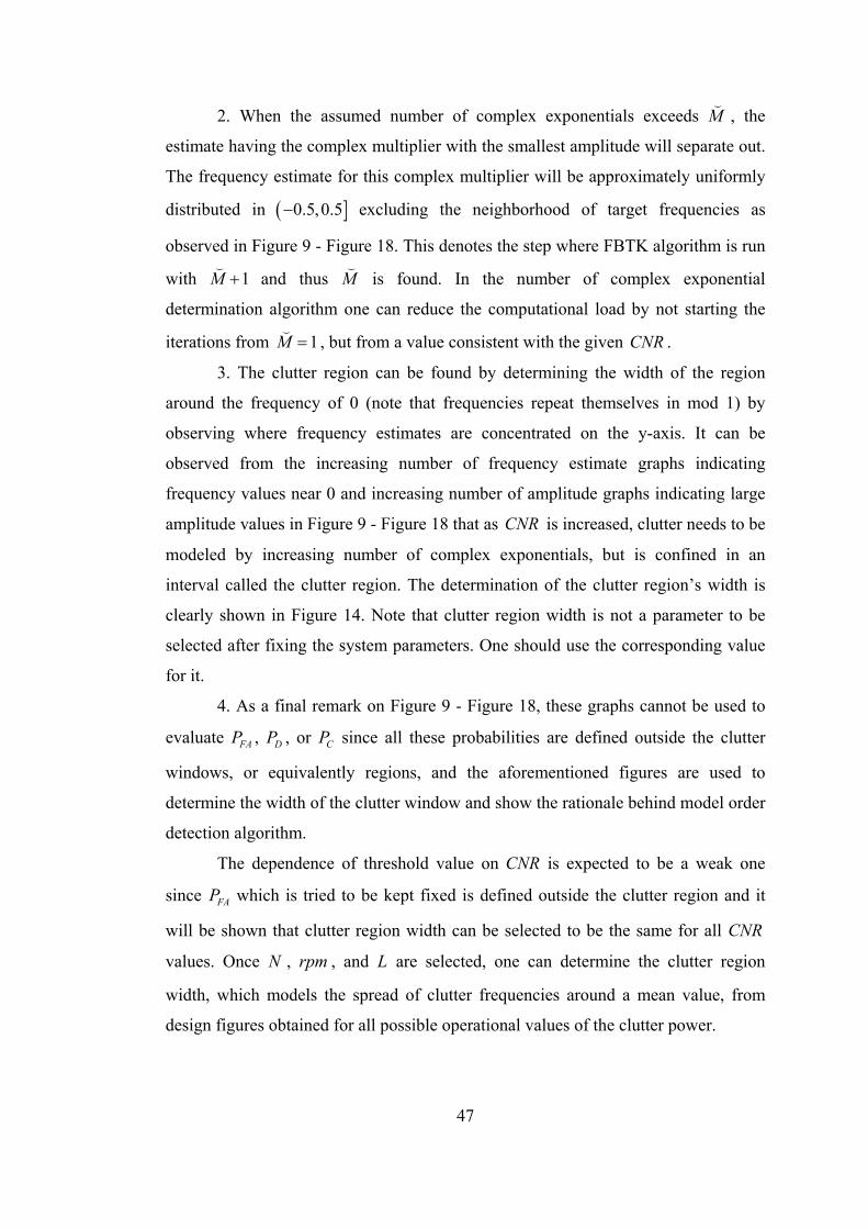
2. When the assumed number of complex exponentials exceeds M , the
estimate having the complex multiplier with the smallest amplitude will separate out.
The frequency estimate for this complex multiplier will be approximately uniformly
distributed in ( ]0.5,0.5− excluding the neighborhood of target frequencies as
observed in Figure 9 - Figure 18. This denotes the step where FBTK algorithm is run
with 1M + and thus M
1
is found. In the number of complex exponential
determination algorithm one can reduce the computational load by not starting the
iterations from M = , but from a value consistent with the given CN . R
3. The clutter region can be found by determining the width of the region
around the frequency of 0 (note that frequencies repeat themselves in mod 1) by
observing where frequency estimates are concentrated on the y-axis. It can be
observed from the increasing number of frequency estimate graphs indicating
frequency values near 0 and increasing number of amplitude graphs indicating large
amplitude values in Figure 9 - Figure 18 that as CN is increased, clutter needs to be
modeled by increasing number of complex exponentials, but is confined in an
interval called the clutter region. The determination of the clutter region’s width is
clearly shown in
R
Figure 14. Note that clutter region width is not a parameter to be
selected after fixing the system parameters. One should use the corresponding value
for it.
4. As a final remark on Figure 9 - Figure 18, these graphs cannot be used to
evaluate , FAP DP , or since all these probabilities are defined outside the clutter
windows, or equivalently regions, and the aforementioned figures are used to
determine the width of the clutter window and show the rationale behind model order
detection algorithm.
CP
The dependence of threshold value on CNR is expected to be a weak one
since which is tried to be kept fixed is defined outside the clutter region and it
will be shown that clutter region width can be selected to be the same for all CNR
values. Once , , and L are selected, one can determine the clutter region
width, which models the spread of clutter frequencies around a mean value, from
design figures obtained for all possible operational values of the clutter power.
FAP
N rpm
47
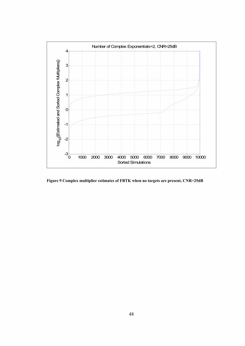
0 1000 2000 3000 4000 5000 6000 7000 8000 9000 10000-3
-2
-1
0
1
2
3
4
Sorted Simulations
log 10
(|Est
imat
ed a
nd S
orte
d C
ompl
ex M
ultip
liers
|)
Number of Complex Exponentials=2, CNR=25dB
Figure 9 Complex multiplier estimates of FBTK when no targets are present, CNR=25dB
48
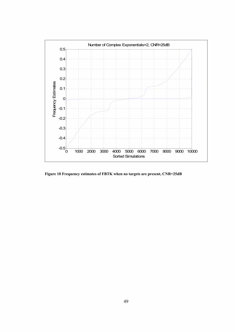
0 1000 2000 3000 4000 5000 6000 7000 8000 9000 10000-0.5
-0.4
-0.3
-0.2
-0.1
0
0.1
0.2
0.3
0.4
0.5
Sorted Simulations
Freq
uenc
y E
stim
ates
Number of Complex Exponentials=2, CNR=25dB
Figure 10 Frequency estimates of FBTK when no targets are present, CNR=25dB
49
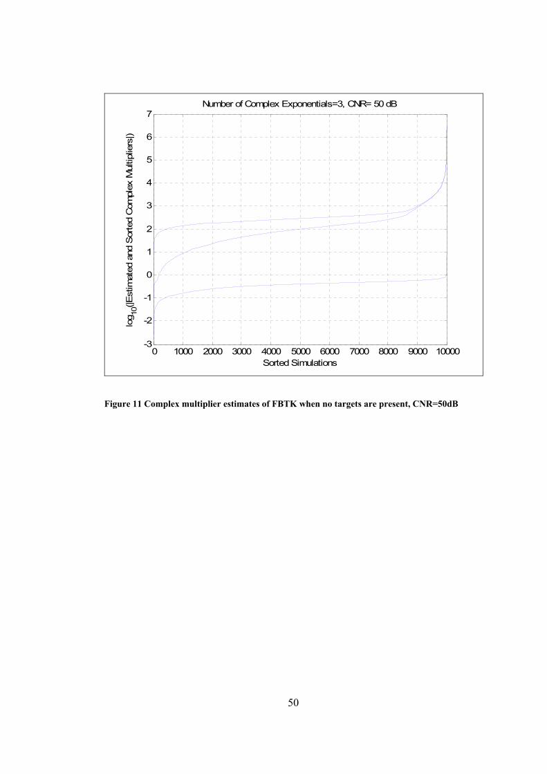
0 1000 2000 3000 4000 5000 6000 7000 8000 9000 10000-3
-2
-1
0
1
2
3
4
5
6
7
Sorted Simulations
log 10
(|Est
imat
ed a
nd S
orte
d C
ompl
ex M
ultip
liers
|)
Number of Complex Exponentials=3, CNR= 50 dB
Figure 11 Complex multiplier estimates of FBTK when no targets are present, CNR=50dB
50

0 1000 2000 3000 4000 5000 6000 7000 8000 9000 10000-0.5
-0.4
-0.3
-0.2
-0.1
0
0.1
0.2
0.3
0.4
0.5Fr
eque
ncy
Est
imat
es
Sorted Simulations
Number of Complex Exponentials=3, CNR=50dB
Figure 12 Frequency estimates of FBTK when no targets are present, CNR=50dB
51
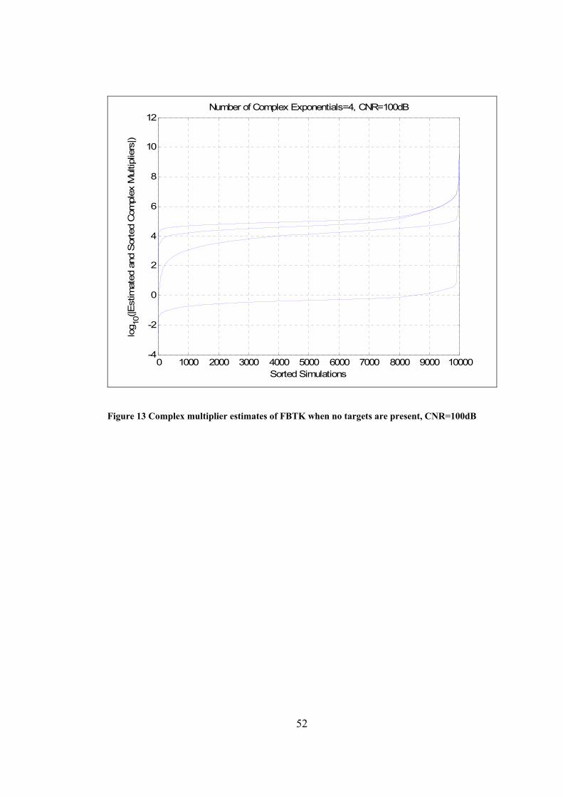
0 1000 2000 3000 4000 5000 6000 7000 8000 9000 10000-4
-2
0
2
4
6
8
10
12
Sorted Simulations
log 10
(|Est
imat
ed a
nd S
orte
d C
ompl
ex M
ultip
liers
|)
Number of Complex Exponentials=4, CNR=100dB
Figure 13 Complex multiplier estimates of FBTK when no targets are present, CNR=100dB
52
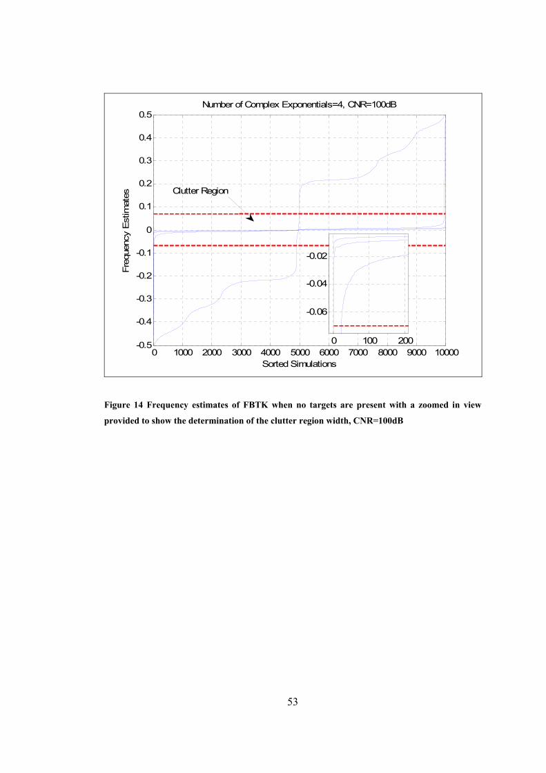
0 1000 2000 3000 4000 5000 6000 7000 8000 9000 10000-0.5
-0.4
-0.3
-0.2
-0.1
0
0.1
0.2
0.3
0.4
0.5Number of Complex Exponentials=4, CNR=100dB
Freq
uenc
y E
stim
ates
Sorted Simulations
Clutter Region
0 100 200
-0.06
-0.04
-0.02
Figure 14 Frequency estimates of FBTK when no targets are present with a zoomed in view
provided to show the determination of the clutter region width, CNR=100dB
53
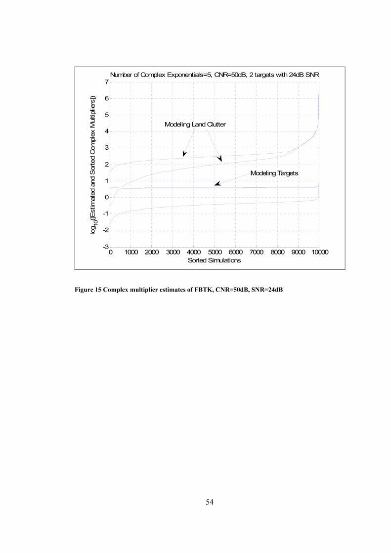
0 1000 2000 3000 4000 5000 6000 7000 8000 9000 10000-3
-2
-1
0
1
2
3
4
5
6
7
Sorted Simulations
log 10
(|Est
imat
ed a
nd S
orte
d C
ompl
ex M
ultip
liers
|)
Number of Complex Exponentials=5, CNR=50dB, 2 targets with 24dB SNR
Modeling Land Clutter
Modeling Targets
Figure 15 Complex multiplier estimates of FBTK, CNR=50dB, SNR=24dB
54
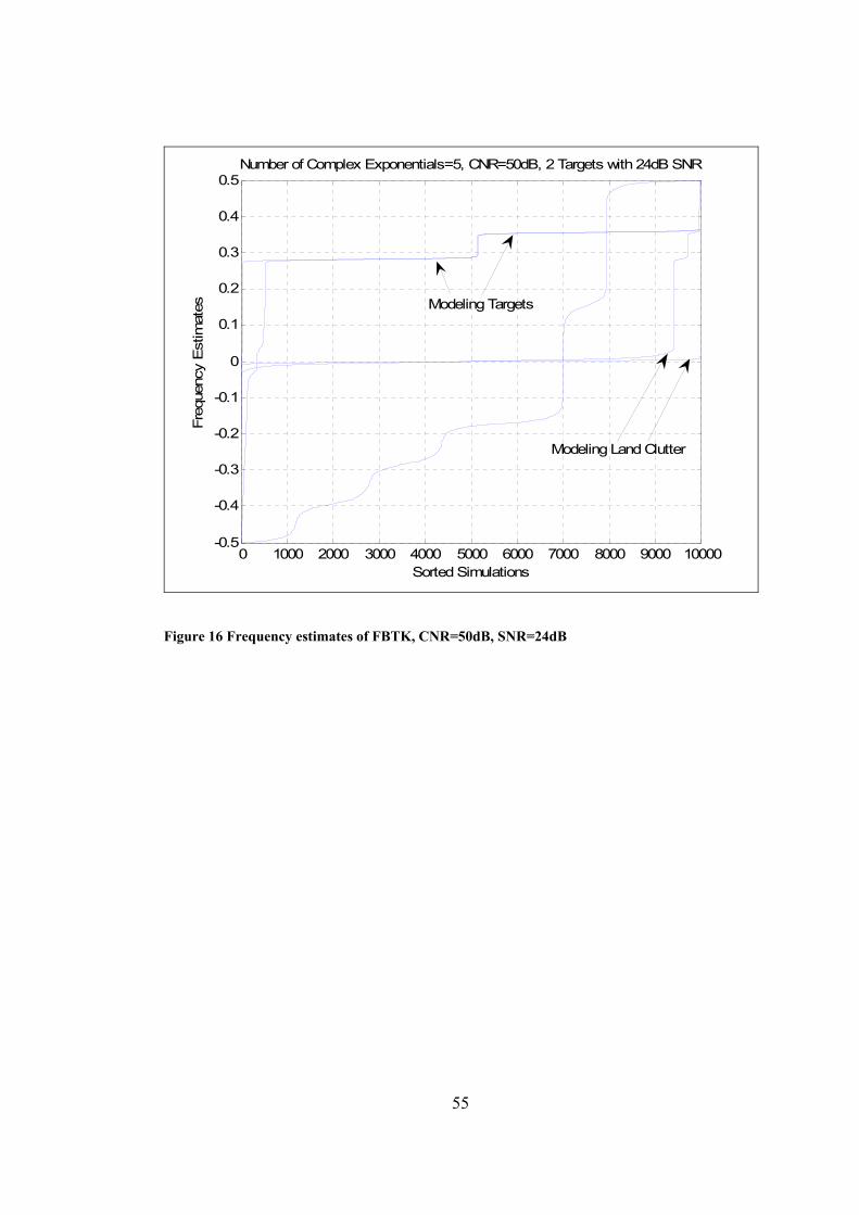
0 1000 2000 3000 4000 5000 6000 7000 8000 9000 10000-0.5
-0.4
-0.3
-0.2
-0.1
0
0.1
0.2
0.3
0.4
0.5Number of Complex Exponentials=5, CNR=50dB, 2 Targets with 24dB SNR
Freq
uenc
y E
stim
ates
Sorted Simulations
Modeling Targets
Modeling Land Clutter
Figure 16 Frequency estimates of FBTK, CNR=50dB, SNR=24dB
55
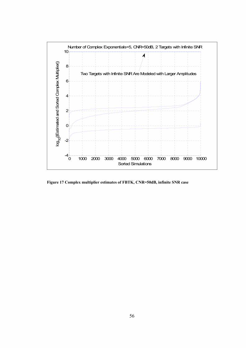
0 1000 2000 3000 4000 5000 6000 7000 8000 9000 10000-4
-2
0
2
4
6
8
10
Sorted Simulations
log 10
(|Est
imat
ed a
nd S
orte
d C
ompl
ex M
ultip
lier|)
Number of Complex Exponentials=5, CNR=50dB, 2 Targets with Infinite SNR
Two Targets with Infinite SNR Are Modeled with Larger Amplitudes
Figure 17 Complex multiplier estimates of FBTK, CNR=50dB, infinite SNR case
56
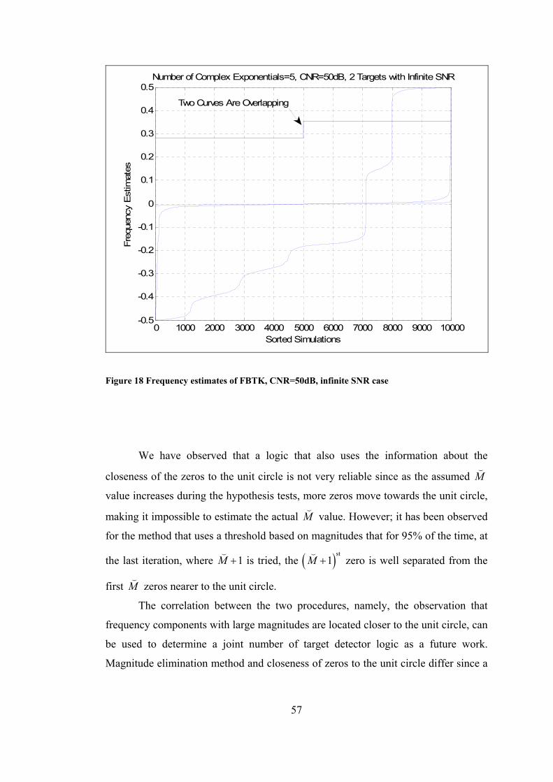
0 1000 2000 3000 4000 5000 6000 7000 8000 9000 10000-0.5
-0.4
-0.3
-0.2
-0.1
0
0.1
0.2
0.3
0.4
0.5
Sorted Simulations
Freq
uenc
y E
stim
ates
Number of Complex Exponentials=5, CNR=50dB, 2 Targets with Infinite SNR
Two Curves Are Overlapping
Figure 18 Frequency estimates of FBTK, CNR=50dB, infinite SNR case
We have observed that a logic that also uses the information about the
closeness of the zeros to the unit circle is not very reliable since as the assumed M
value increases during the hypothesis tests, more zeros move towards the unit circle,
making it impossible to estimate the actual M value. However; it has been observed
for the method that uses a threshold based on magnitudes that for 95% of the time, at
the last iteration, where 1M + is tried, the ( )st1+M zero is well separated from the
first M zeros nearer to the unit circle.
The correlation between the two procedures, namely, the observation that
frequency components with large magnitudes are located closer to the unit circle, can
be used to determine a joint number of target detector logic as a future work.
Magnitude elimination method and closeness of zeros to the unit circle differ since a
57

second or third clutter zero can be the one farthest from the unit circle among the
selected zeros, while it results in a large magnitude since very closely spaced
complex exponentials result in high amplitude levels when least squares method is
used in amplitude determination.
Procedure to decide on M and M is not repeated for each high resolution
line component estimation technique, but the results obtained from using FBTK are
used in other algorithms. This is to ensure same level of noise reduction in all
algorithms and compare their effectiveness under given M .
58
CHAPTER 8
LTI MAXSIR FILTER DESIGN FOR LAND CLUTTER
In this chapter, we will investigate possibilities on whether there exists pre-
processing algorithms that can improve the performance of FBTK algorithm.
When one pre-whitens the data through the transformation
( )1
2n −=y R x , (8.1)
y with its samples cannot be processed directly with the FBTK algorithm to
obtain the frequencies of the targets because the complex exponential model of x is
not preserved with this transformation.
N
We will derive the optimal linear time-invariant (LTI) filter in terms of
maximization when the Doppler frequency of the target is known to lie in a
certain interval and show that its presence cannot improve the estimation results
obtained by LP. We have chosen an LTI filter so that the input frequency
components will be observed at the output with possibly amplitude and phase
distortion. Since one cannot do much when the target is in the clutter region, the
interval in which the frequencies of targets should lie will be chosen as uniform
distribution outside the land clutter region.
SCNR
In order to satisfy the WSS condition, one can use only number of
samples at the output of the designed filter u , i.e., the transient samples at both ends
should be discarded and only the samples resulting from parts of x and fully
overlapping should be used. Let us assume that phases of complex multipliers of
targets are uncorrelated and uniformly distributed in
1N K− +
u
( ],π π− . Also, complex
exponential frequencies iω ’s modeling targets are taken to be uniformly distributed
in , ,π ππ πβ β
⎛ ⎞ ⎛−− ∪⎜ ⎟ ⎜ ⎥⎝ ⎠ ⎝
⎤
⎦. We define the optimum filter as u
59
[ ]0T
Ku u −=u 1 (8.2)
and, considering equations (2.5) and (3.14), s as
[ ]0T
Ns s −= =Va s 1 . (8.3)
Output signal energy from the filter is
{ }( ) (
1
21 1
1 0, , ,
1 1 *0 0
1
M
N Kk i ki K k
K Kk m Mk m
E u s
N K u u f m k
ω ω
− −
−= − =
− −
= == − + −
∑ ∑
∑ ∑a…
) (8.4)
where
( ) ( )( )( ) ( )
,
sin sinconstant M,M
m k m kf m k
m kβ
ππβ
β
⎛ ⎞− − −⎜ ⎟
⎝− =−
⎠ (8.5)
while the output clutter energy is
{ }{
( )
21 1
1 0
1 1 1 * *1 0 0
1 1 1 *1 0 0
N Kk i ki K k
N K Kk m i k i mi K k m
N K K nk mi K k m
E u n
E u u
u u R m k
− −
−= − =
− − −
− −= − = =
− − −
= − = =
=
= −
∑ ∑
∑ ∑ ∑∑ ∑ ∑
}n n (8.6)
where is the autocorrelation sequence of the colored noise. ( )nR i
Passing to the vector-matrix notation, the problem becomes the maximization
of the Lagrangian
( ) ( ),H M H n cβ λΛ = − −u u F u u R u (8.7)
where
( ),, ,
Mm k Mf m kβ
β= −F . (8.8)
The solution can be obtained as follows:
( )( )( )
*
,
1 ,
1 ,
M n
n M
n M
β
β
β
λ
λ
λ
−
−
∇ Λ =
− =
− =
− =
u0
F u R u 0
R F u u
R F I u
0
0
. (8.9)
From the last equation it is clear that optimal u is an eigenvector of ( ) 1n β−R F ,
where it is evident that the constant in equation (8.5) is of no importance and thus
60
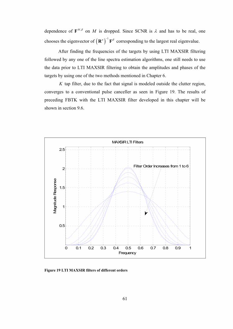
dependence of ,M βF on M is dropped. Since SCNR is λ and has to be real, one
chooses the eigenvector of ( ) 1n β−R F corresponding to the largest real eigenvalue.
After finding the frequencies of the targets by using LTI MAXSIR filtering
followed by any one of the line spectra estimation algorithms, one still needs to use
the data prior to LTI MAXSIR filtering to obtain the amplitudes and phases of the
targets by using one of the two methods mentioned in Chapter 6.
K tap filter, due to the fact that signal is modeled outside the clutter region,
converges to a conventional pulse canceller as seen in Figure 19. The results of
preceding FBTK with the LTI MAXSIR filter developed in this chapter will be
shown in section 9.6.
61
0 0.1 0.2 0.3 0.4 0.5 0.6 0.7 0.8 0.9 1
0.5
1
1.5
2
2.5
Frequency
Mag
nitu
de R
espo
nse
MAXSIR LTI Filters
Filter Order eases from 1 to 6 Incr
Figure 19 LTI MAXSIR filters of different orders
CHAPTER 9
SIMULATION RESULTS
In this chapter we present the results pertaining to performances of the
various algorithms discussed so far. The results have been obtained using Monte-
Carlo simulations.
9.1. Simulation Parameters
Unless otherwise stated, the default simulation parameters are as follows: 4
230, 1.2728 , 10 , 16, 9, 45 , 2, 24 ,WHPrpm PRI s N L CNR dB M SNR dBθ ° ° −= = = = = = = =
[ ] [ ]1 2 0.2813 0.3563 , 5 , 0.7688 and number of simulations=cf f MCCR dB f= = − =2WN10000. In the simulations the noise power σ is kept fixed at 1. SNR or CNR is
varied to obtain the necessary graphs. Both of the targets are assumed to have the
same fixed SNR , thus same fixed amplitude, throughout the simulations and phases
of the targets are uniformly distributed in [ )0, 2π and random phase values are used
in each simulation.
Moving clutter will be considered in Chapter 10, so the results in this chapter
include only the land clutter. The results are expected to be the same for moving
clutter since the only difference in their models (see Chapter 2) is that land clutter is
centered at zero frequency.
Clutter region width does not depend on CN or R 2WNσ and as can be
interpreted from design graphs suited to our selected parameters and depicted in
Figure 9 - Figure 18, where all possible clutter powers of interest are considered,
taking its width to be ±0.07 around its center is considered to be a good choice for
the selected parameters.
Table 1 gives the number of detections of the FBTK method that are outside
the clutter region, and thus identified as targets, for various SNR levels. 2M = is
62
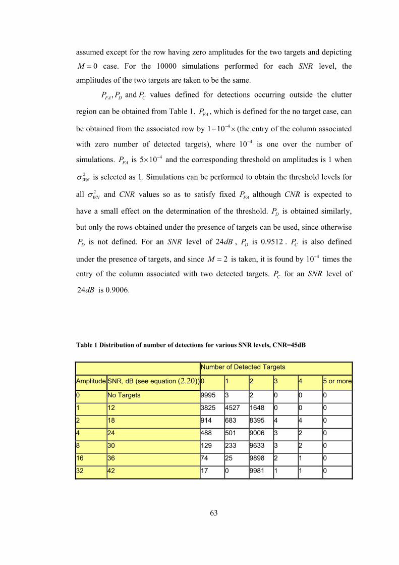
assumed except for the row having zero amplitudes for the two targets and depicting
case. For the 10000 simulations performed for each level, the
amplitudes of the two targets are taken to be the same.
0M = SNR
, and FA D CP P P values defined for detections occurring outside the clutter
region can be obtained from Table 1. , which is defined for the no target case, can
be obtained from the associated row by
FAP
41 10−− × (the entry of the column associated
with zero number of detected targets), where 410− is one over the number of
simulations. is and the corresponding threshold on amplitudes is 1 when FAP × 45 10−
2WNσ is selected as 1. Simulations can be performed to obtain the threshold levels for
all 2WNσ and values so as to satisfy fixed although is expected to
have a small effect on the determination of the threshold.
CNR FAP CNR
DP is obtained similarly,
but only the rows obtained under the presence of targets can be used, since otherwise
DP is not defined. For an SNR level of , 24dB DP is . is also defined
under the presence of targets, and since
0.9512 CP
2M = is taken, it is found by times the
entry of the column associated with two detected targets. for an level of
is 0.9006.
4
R
10−
SNCP
24dB
Table 1 Distribution of number of detections for various SNR levels, CNR=45dB
Number of Detected Targets
Amplitude SNR, dB (see equation (2.20)) 0 1 2 3 4 5 or more
0 No Targets 9995 3 2 0 0 0
1 12 3825 4527 1648 0 0 0
2 18 914 683 8395 4 4 0
4 24 488 501 9006 3 2 0
8 30 129 233 9633 3 2 0
16 36 74 25 9898 2 1 0
32 42 17 0 9981 1 1 0
63
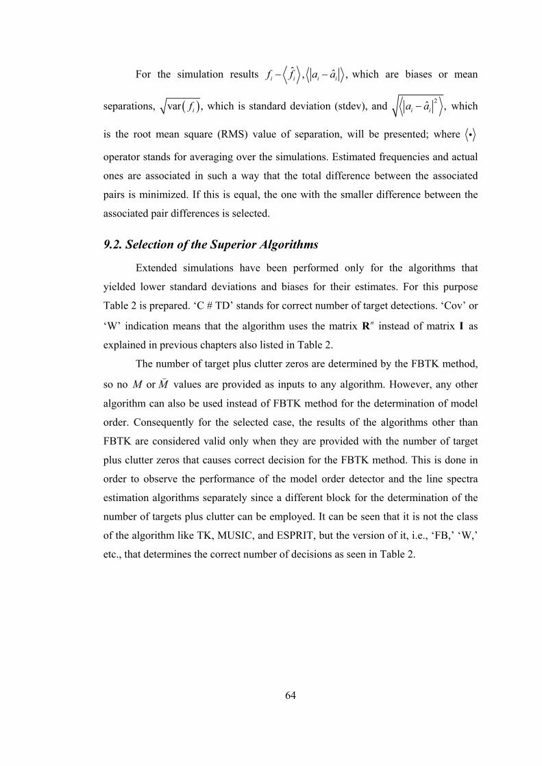
For the simulation results ˆ ˆ,i i i i ,f f a a− − which are biases or mean
separations, ( )var ,if which is standard deviation (stdev), and 2ˆ ,i ia a− which
is the root mean square (RMS) value of separation, will be presented; where i
operator stands for averaging over the simulations. Estimated frequencies and actual
ones are associated in such a way that the total difference between the associated
pairs is minimized. If this is equal, the one with the smaller difference between the
associated pair differences is selected.
9.2. Selection of the Superior Algorithms
Extended simulations have been performed only for the algorithms that
yielded lower standard deviations and biases for their estimates. For this purpose
Table 2 is prepared. ‘C # TD’ stands for correct number of target detections. ‘Cov’ or
‘W’ indication means that the algorithm uses the matrix instead of matrix I as
explained in previous chapters also listed in
nR
Table 2.
The number of target plus clutter zeros are determined by the FBTK method,
so no or M M values are provided as inputs to any algorithm. However, any other
algorithm can also be used instead of FBTK method for the determination of model
order. Consequently for the selected case, the results of the algorithms other than
FBTK are considered valid only when they are provided with the number of target
plus clutter zeros that causes correct decision for the FBTK method. This is done in
order to observe the performance of the model order detector and the line spectra
estimation algorithms separately since a different block for the determination of the
number of targets plus clutter can be employed. It can be seen that it is not the class
of the algorithm like TK, MUSIC, and ESPRIT, but the version of it, i.e., ‘FB,’ ‘W,’
etc., that determines the correct number of decisions as seen in Table 2.
64
Table 2 Performance of all the algorithms for the selected operating condition
f1 stdev f1 bias f2 stdev f2 bias C # TD
FTK (see section 4.3.) 2,41E-02 1,67E-03 1,61E-02 -1,01E-03 2810
BTK 1,28E-02 8,42E-04 1,89E-02 -1,09E-03 2802
FBTK 2,73E-03 3,08E-05 2,80E-03 -2,33E-04 9017
FBTK, NRDV 2,74E-03 -4,13E-05 2,82E-03 9,70E-05 9014
FBTK + ML (see sections 3.2., 4.3.) 2,29E-03 -7,77E-05 2,28E-03 2,75E-05 9017
M (see sub-sections 5.2.2., 5.2.3.) 4,27E-03 1,37E-04 1,37E-02 -6,08E-04 3567
M, FB 3,25E-03 -1,28E-04 3,15E-03 1,33E-04 9010
M, W 7,38E-03 -2,50E-05 1,97E-02 -1,22E-03 8617
M, WFB 8,47E-03 -2,08E-05 1,72E-02 -8,04E-04 7721
M, W (Clutter Counted as Target) 4,33E-02 2,74E-01 1,48E-01 1,16E-01 9017
M, WFB (Clutter Counted as Target) 1,25E-01 7,72E-02 3,21E-02 8,50E-03 9017
Esp (see sub-section 5.4.2.) 4,77E-03 -1,99E-04 4,58E-03 2,12E-05 5576
Esp, FB 3,16E-03 -9,80E-05 3,16E-03 1,04E-04 9016
Esp, Cov 2,93E-02 1,85E-03 3,79E-02 -5,78E-03 1056
Esp, Cov FB 3,96E-02 2,84E-03 3,74E-02 -5,69E-03 2963
Esp, Cov (Clutter Counted as Target) 3,21E-02 2,66E-01 1,47E-02 8,35E-03 9017
Esp, Cov FB (Clutter Counted as Target) 6,61E-02 2,40E-01 3,64E-02 2,10E-02 9017
HWMAXSIR (see section 3.1.) 3,04E-02 -7,21E-03 9,49E-03 -1,73E-02 9017
HWMTI 2,88E-02 -1,22E-02 0,00E+00 -1,88E-02 9017
HWMTI_11 1,62E-02 1,04E-02 3,14E-02 6,45E-04 9016
HWMTI_121 3,03E-02 -1,84E-02 2,89E-02 -1,57E-02 9017
CR Bound, ML (see sections 3.2., 3.3.) 8,17E-04 0,00E+00 8,12E-04 0,00E+00
Standard deviation and mean estimates are obtained from variable number of
simulations. We do so because discarding some samples in calculations is not
meaningful although this results in variable confidence intervals. We shall note that
confidence intervals decrease with the number of considered simulations [34] - [36],
i.e., those that yield correct number of target detections. For the results that are
65
presented, ten thousand simulations are made and only those that yield correct
number of target estimations are used in obtaining the figures.
We have used the MATLAB function fminunc, which solves unconstrained
optimization problems by finding the minimum of the cost functions, without
providing Gradient or Hessian information (see Appendix A) except for the cases of
low or closely spaced complex exponential frequencies. The results are just
indicative of the fact that estimates can be improved with ML processing.
SNR
Only five of the algorithms presented in Table 2 will be considered for further
analysis because they yield the lower biases and standard deviations. Namely, they
are FBTK, ‘FBTK, NRDV,’ ‘FBTK + ML,’ ‘M, FB,’ and ‘Esp, FB’. We can observe
that ‘W’ or ‘Cov’ versions of the algorithms require to run with M rather than M
and employ the clutter region concept for better estimates. However, we can
conclude from the simulations that these versions of the algorithms are inferior to the
versions that do not use the actual clutter plus noise autocorrelation matrix and
consider the clutter as additional number of targets and formulate the problem in
white noise.
Considering the computational complexities of the selected algorithms,
although not conclusive in any sense, time consumption of the algorithms can be
ordered from lowest to highest as ‘Esp, FB,’ FBTK, ‘FBTK, NRDV,’ and ‘M, FB’.
9.3. Analysis of Linear Prediction and FBTK Algorithm
Linear prediction uses the autocorrelation matrix of the clutter plus noise, not
the actual observation vector. Thus, we call it Ideal LP. As a result, the estimates will
not have any variation, but only a bias. As can be seen from Figure 20, this bias
decreases with the order of L ( )IdealH z in equation (4.4). This bias may result from
the zeros of targets, clutter, and noise affecting each other’s position.
66
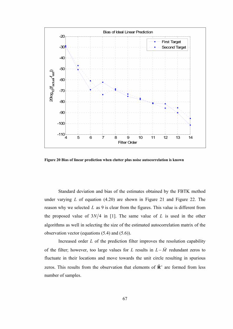
4 5 6 7 8 9 10 11 12 13 14-110
-100
-90
-80
-70
-60
-50
-40
-30
-20
20lo
g 10(|f
actu
al-f es
t|)
Filter Order
Bias of Ideal Linear Prediction
First TargetSecond Target
Figure 20 Bias of linear prediction when clutter plus noise autocorrelation is known
Standard deviation and bias of the estimates obtained by the FBTK method
under varying of equation L (4.20) are shown in Figure 21 and Figure 22. The
reason why we selected as 9 is clear from the figures. This value is different from
the proposed value of
L
3N 4 in [1]. The same value of is used in the other
algorithms as well in selecting the size of the estimated autocorrelation matrix of the
observation vector (equations
L
(5.4) and (5.6)).
Increased order L of the prediction filter improves the resolution capability
of the filter; however, too large values for L results in L M−
ˆ
redundant zeros to
fluctuate in their locations and move towards the unit circle resulting in spurious
zeros. This results from the observation that elements of xR are formed from less
number of samples.
67
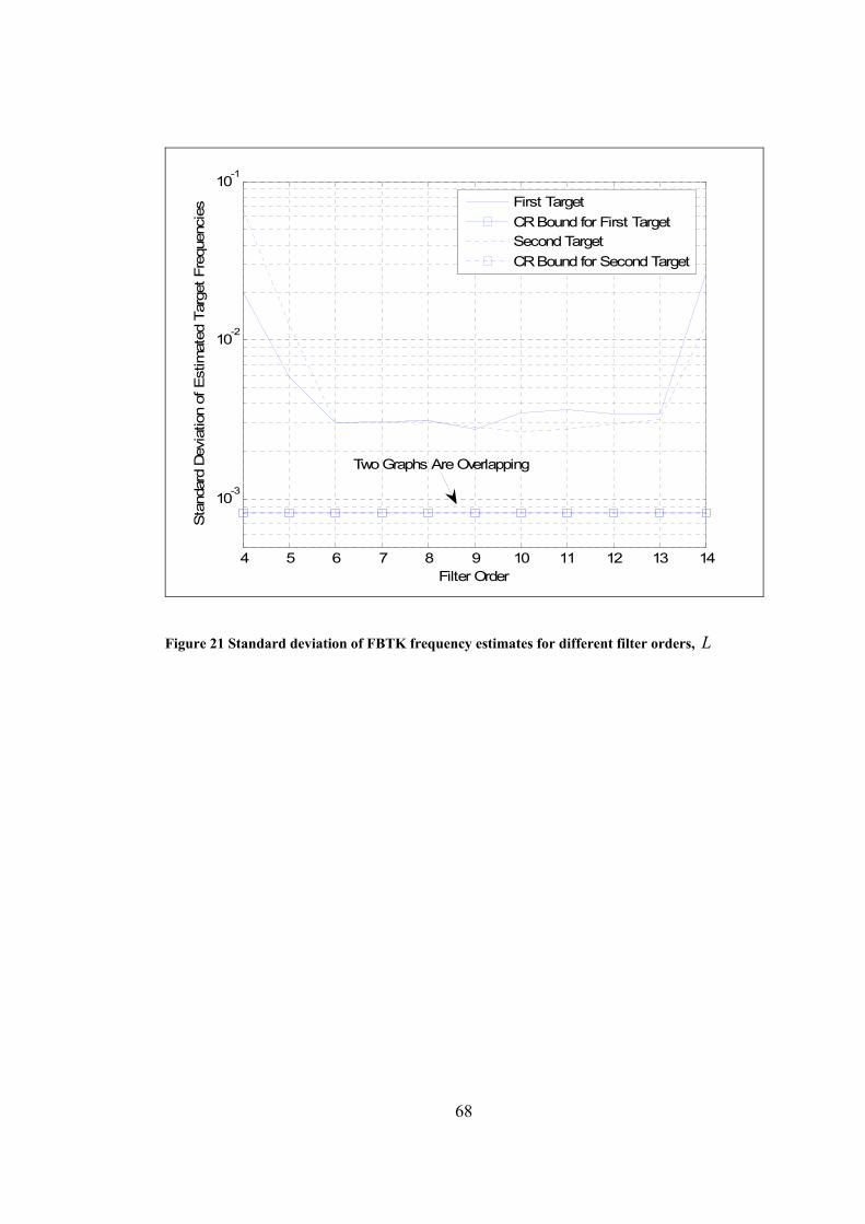
4 5 6 7 8 9 10 11 12 13 14
10-3
10-2
10-1
Filter Order
Sta
ndar
d D
evia
tion
of E
stim
ated
Tar
get F
requ
enci
esFirst TargetCR Bound for First TargetSecond TargetCR Bound for Second Target
Two Graphs Are Overlapping
Figure 21 Standard deviation of FBTK frequency estimates for different filter orders, L
68
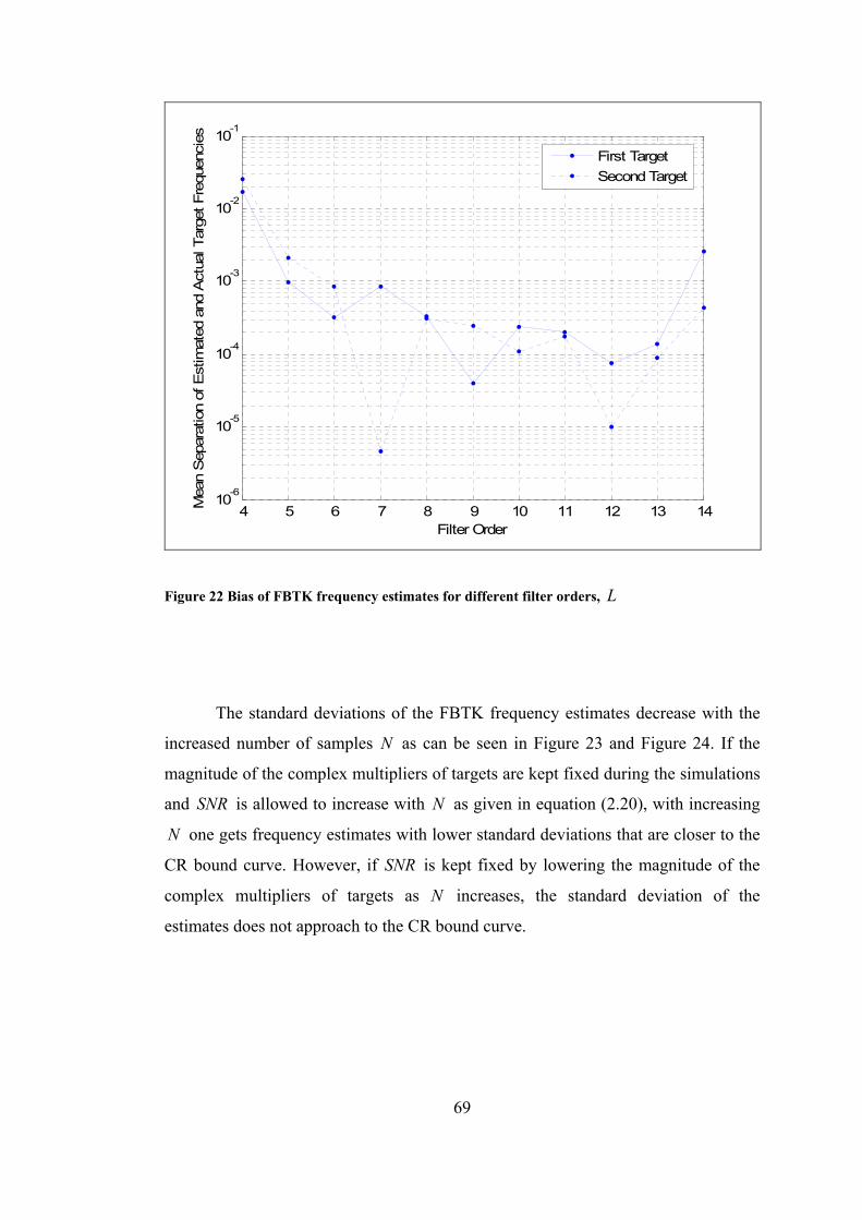
4 5 6 7 8 9 10 11 12 13 1410-6
10-5
10-4
10-3
10-2
10-1
Filter Order
Mea
n S
epar
atio
n of
Est
imat
ed a
nd A
ctua
l Tar
get F
requ
enci
es
First TargetSecond Target
Figure 22 Bias of FBTK frequency estimates for different filter orders, L
The standard deviations of the FBTK frequency estimates decrease with the
increased number of samples N as can be seen in Figure 23 and Figure 24. If the
magnitude of the complex multipliers of targets are kept fixed during the simulations
and is allowed to increase with as given in equation SNR N (2.20), with increasing
one gets frequency estimates with lower standard deviations that are closer to the
CR bound curve. However, if SNR is kept fixed by lowering the magnitude of the
complex multipliers of targets as N increases, the standard deviation of the
estimates does not approach to the CR bound curve.
N
69
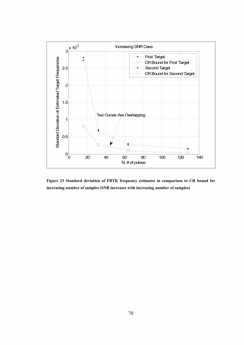
0 20 40 60 80 100 120 1400
0.5
1
1.5
2
2.5
3x 10⁻³
N, # of pulses
Sta
ndar
d D
evia
tion
of E
stim
ated
Tar
get F
requ
enci
es
Increasing SNR Case
First TargetCR Bound for First TargetSecond TargetCR Bound for Second Target
Two Curves Are Overlapping
Figure 23 Standard deviation of FBTK frequency estimates in comparison to CR bound for
increasing number of samples (SNR increases with increasing number of samples)
70
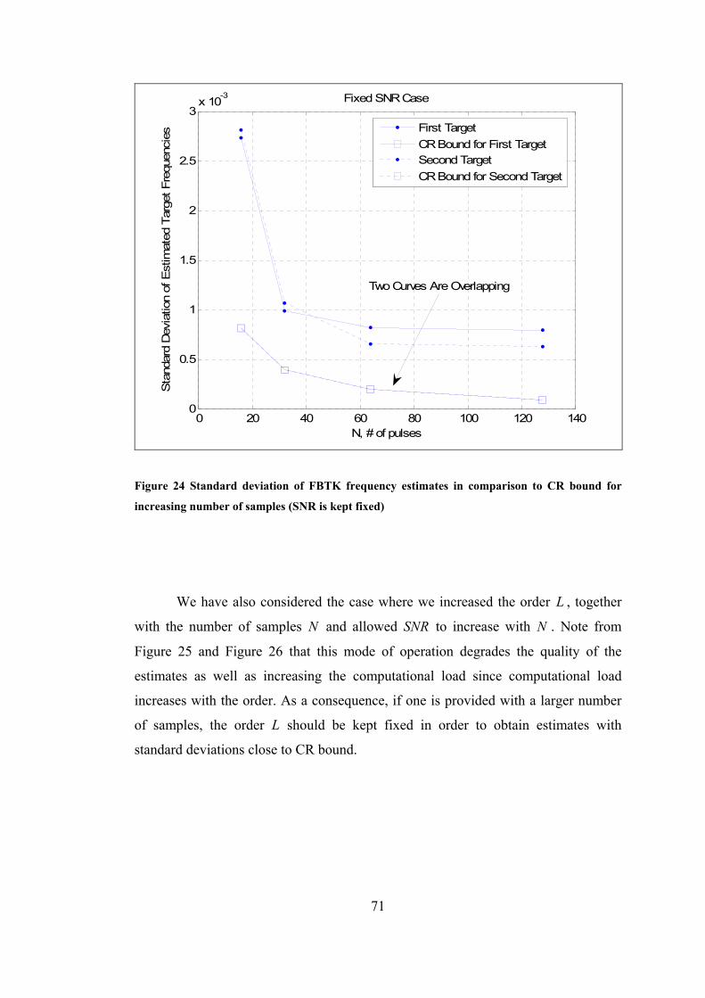
0 20 40 60 80 100 120 1400
0.5
1
1.5
2
2.5
3x 10⁻³
N, # of pulses
Sta
ndar
d D
evia
tion
of E
stim
ated
Tar
get F
requ
enci
es
Fixed SNR Case
First TargetCR Bound for First TargetSecond TargetCR Bound for Second Target
Two Curves Are Overlapping
Figure 24 Standard deviation of FBTK frequency estimates in comparison to CR bound for
increasing number of samples (SNR is kept fixed)
We have also considered the case where we increased the order L , together
with the number of samples and allowed to increase with N . Note from N SNR
Figure 25 and Figure 26 that this mode of operation degrades the quality of the
estimates as well as increasing the computational load since computational load
increases with the order. As a consequence, if one is provided with a larger number
of samples, the order L should be kept fixed in order to obtain estimates with
standard deviations close to CR bound.
71
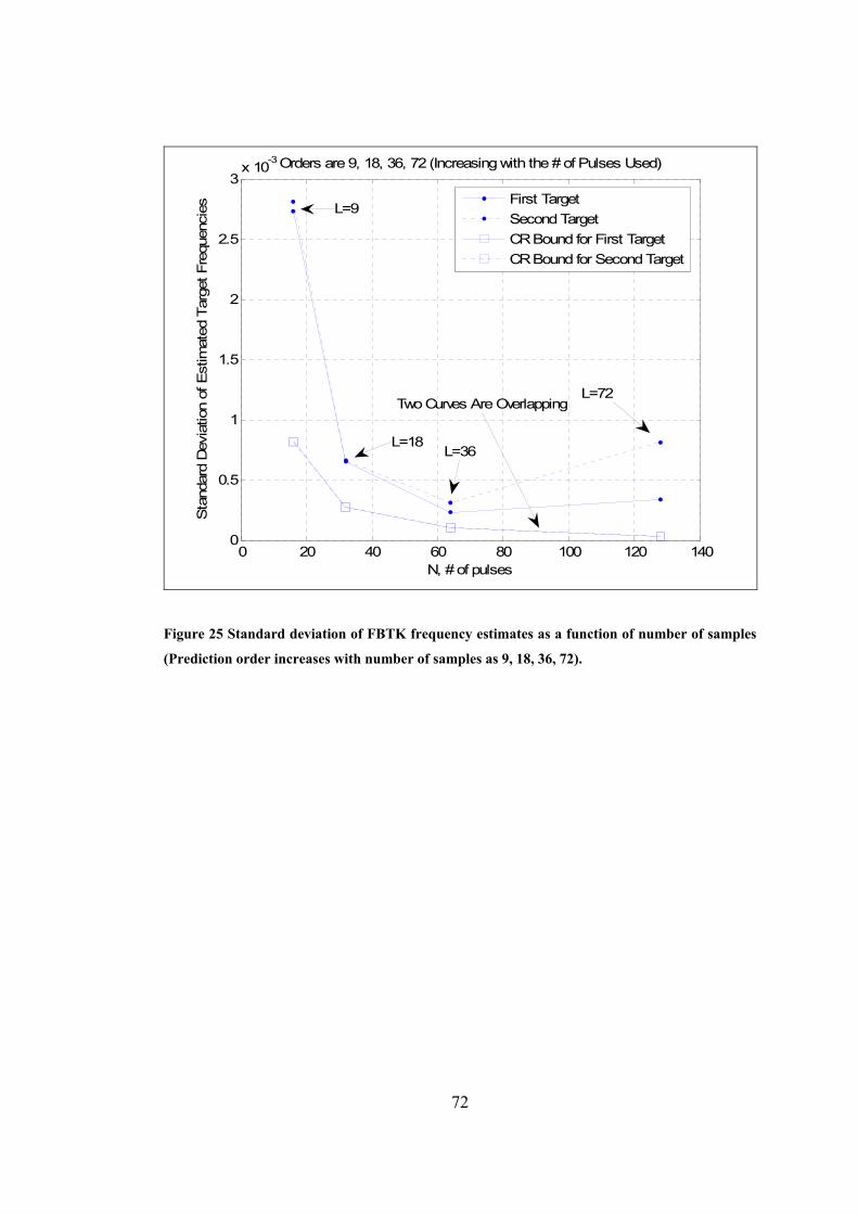
0 20 40 60 80 100 120 1400
0.5
1
1.5
2
2.5
3x 10⁻³
N, # of pulses
Sta
ndar
d D
evia
tion
of E
stim
ated
Tar
get F
requ
enci
es
Orders are 9, 18, 36, 72 (Increasing with the # of Pulses Used)
First TargetSecond TargetCR Bound for First TargetCR Bound for Second Target
L=9
L=18L=36
L=72Two Curves Are Overlapping
Figure 25 Standard deviation of FBTK frequency estimates as a function of number of samples
(Prediction order increases with number of samples as 9, 18, 36, 72).
72
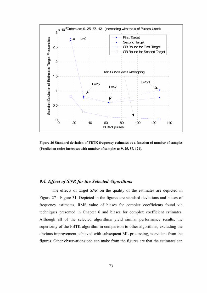
0 20 40 60 80 100 120 1400
0.5
1
1.5
2
2.5
3x 10⁻³
N, # of pulses
Sta
ndar
d D
evia
tion
of E
stim
ated
Tar
get F
requ
enci
es
Orders are 9, 25, 57, 121 (Increasing with the # of Pulses Used)
First TargetSecond TargetCR Bound for First TargetCR Bound for Second Target
L=9
L=25L=57
L=121
Two Curves Are Overlapping
Figure 26 Standard deviation of FBTK frequency estimates as a function of number of samples
(Prediction order increases with number of samples as 9, 25, 57, 121).
9.4. Effect of SNR for the Selected Algorithms
The effects of target SN on the quality of the estimates are depicted in R
Figure 27 - Figure 31. Depicted in the figures are standard deviations and biases of
frequency estimates, RMS value of biases for complex coefficients found via
techniques presented in Chapter 6 and biases for complex coefficient estimates.
Although all of the selected algorithms yield similar performance results, the
superiority of the FBTK algorithm in comparison to other algorithms, excluding the
obvious improvement achieved with subsequent ML processing, is evident from the
figures. Other observations one can make from the figures are that the estimates can
73

be considered unbiased and there is no improvement achieved with the ‘FBTK,
NRDV’ algorithm.
CR bounds shown in the figures have been derived under the assumption of
unbiased estimates and the figures showing the bias of the estimates are given to
verify this assumption.
10 15 20 25 30 35 40 4510-4
10-3
10-2
SNR, dB
Sta
ndar
d D
evia
tion
of F
irst T
arge
t's E
stim
ated
Fre
quen
cy Esp, FBM, FBFBTKFBTK, NRDVTK + MLCR Bound
Figure 27 Standard deviation of the first target’s frequency estimate of selected methods with
SNR
74
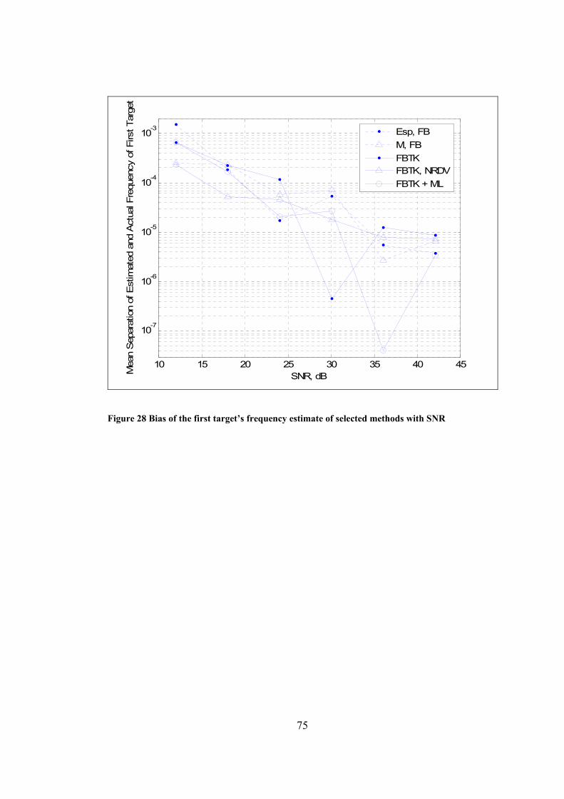
10 15 20 25 30 35 40 45
10-7
10-6
10-5
10-4
10-3
SNR, dBMea
n S
epar
atio
n of
Est
imat
ed a
nd A
ctua
l Fre
quen
cy o
f Firs
t Tar
get
Esp, FBM, FBFBTKFBTK, NRDVFBTK + ML
Figure 28 Bias of the first target’s frequency estimate of selected methods with SNR
75
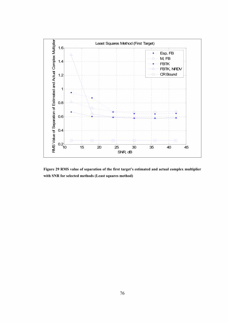
10 15 20 25 30 35 40 450.2
0.4
0.6
0.8
1
1.2
1.4
1.6
SNR, dBRM
S V
alue
of S
epar
atio
n of
Est
imat
ed a
nd A
ctua
l Com
plex
Mul
tiplie
r
Least Squares Method (First Target)
Esp, FBM, FBFBTKFBTK, NRDVCR Bound
Figure 29 RMS value of separation of the first target’s estimated and actual complex multiplier
with SNR for selected methods (Least squares method)
76
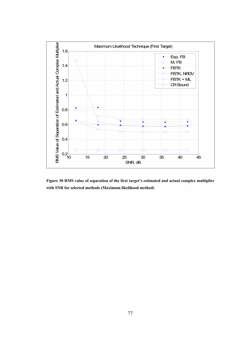
10 15 20 25 30 35 40 450.2
0.4
0.6
0.8
1
1.2
1.4
1.6
SNR, dBRM
S V
alue
of S
epar
atio
n of
Est
imat
ed a
nd A
ctua
l Com
plex
Mul
tiplie
r
Maximum Likelihood Technique (First Target)
Esp, FBM, FBFBTKFBTK, NRDVFBTK + MLCR Bound
Figure 30 RMS value of separation of the first target’s estimated and actual complex multiplier
with SNR for selected methods (Maximum likelihood method)
77
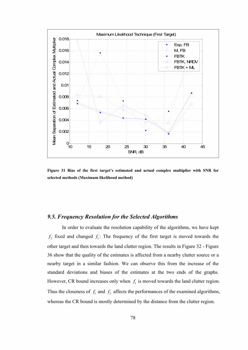
10 15 20 25 30 35 40 450
0.002
0.004
0.006
0.008
0.01
0.012
0.014
0.016
0.018
SNR, dB
Maximum Likelihood Technique (First Target)
Mea
n S
epar
atio
n of
Est
imat
ed a
nd A
ctua
l Com
plex
Mul
tiplie
r
Esp, FBM, FBFBTKFBTK, NRDVFBTK + ML
Figure 31 Bias of the first target’s estimated and actual complex multiplier with SNR for
selected methods (Maximum likelihood method)
9.5. Frequency Resolution for the Selected Algorithms
In order to evaluate the resolution capability of the algorithms, we have kept
2f fixed and changed 1f : The frequency of the first target is moved towards the
other target and then towards the land clutter region. The results in Figure 32 - Figure
36 show that the quality of the estimates is affected from a nearby clutter source or a
nearby target in a similar fashion. We can observe this from the increase of the
standard deviations and biases of the estimates at the two ends of the graphs.
However, CR bound increases only when 1f is moved towards the land clutter region.
Thus the closeness of 1f an 2d f affects the performances of the examined algorithms,
whereas the CR bound is mostly determined by the distance from the clutter region.
78
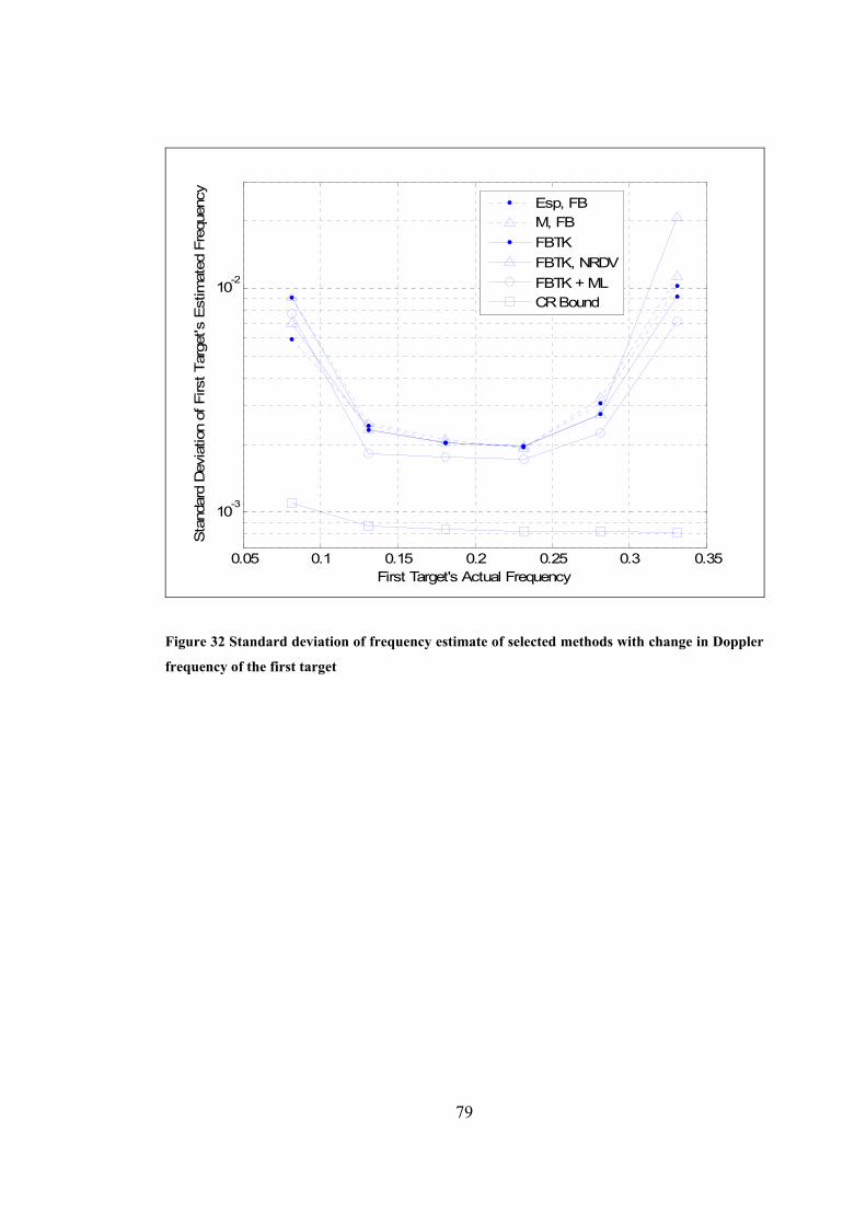
0.05 0.1 0.15 0.2 0.25 0.3 0.35
10-3
10-2
First Target's Actual Frequency
Sta
ndar
d D
evia
tion
of F
irst T
arge
t's E
stim
ated
Fre
quen
cy Esp, FBM, FBFBTKFBTK, NRDVFBTK + MLCR Bound
Figure 32 Standard deviation of frequency estimate of selected methods with change in Doppler
equency of the first target
fr
79
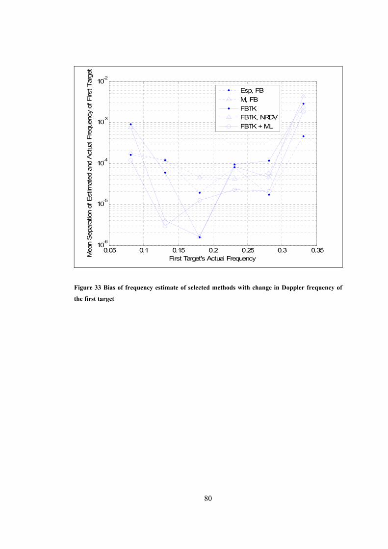
0.05 0.1 0.15 0.2 0.25 0.3 0.3510-6
10-5
10-4
10-3
10-2
First Target's Actual FrequencyMea
n S
epar
atio
n of
Est
imat
ed a
nd A
ctua
l Fre
quen
cy o
f Firs
t Tar
get
Esp, FBM, FBFBTKFBTK, NRDVFBTK + ML
Figure 33 Bias of frequency estimate of selected methods with change in Doppler frequency of
e first target
th
80
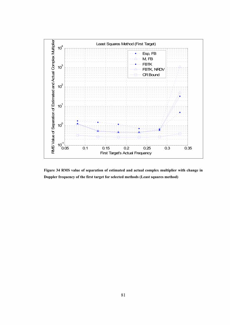
0.05 0.1 0.15 0.2 0.25 0.3 0.3510-1
100
101
102
103
104
First Target's Actual FrequencyRM
S V
alue
of S
epar
atio
n of
Est
imat
ed a
nd A
ctua
l Com
plex
Mul
tiplie
r
Least Squares Method (First Target)
Esp, FBM, FBFBTKFBTK, NRDVCR Bound
Figure 34 RMS value of separation of estimated and actual complex multiplier with change in
oppler frequency of the first target for selected methods (Least squares method)
D
81
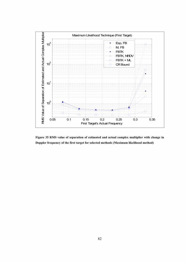
0.05 0.1 0.15 0.2 0.25 0.3 0.35
100
101
102
103
First Target's Actual FrequencyRM
S V
alue
of S
epar
atio
n of
Est
imat
ed a
nd A
ctua
l Com
plex
Mul
tiplie
r
Maximum Likelihood Technique (First Target)
Esp, FBM, FBFBTKFBTK, NRDVFBTK + MLCR Bound
Figure 35 RMS value of separation of estimated and actual complex multiplier with change in
oppler frequency of the first target for selected methods (Maximum likelihood method)
D
82
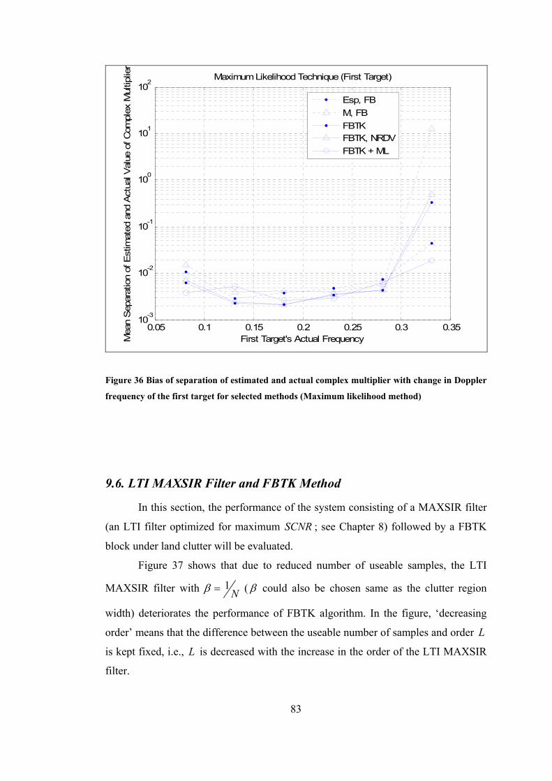
0.05 0.1 0.15 0.2 0.25 0.3 0.3510-3
10-2
10-1
100
101
102
First Target's Actual FrequencyMea
n S
epar
atio
n of
Est
imat
ed a
nd A
ctua
l Val
ue o
f Com
plex
Mul
tiplie
r
Maximum Likelihood Technique (First Target)
Esp, FBM, FBFBTKFBTK, NRDVFBTK + ML
Figure 36 Bias of separation of estimated and actual complex multiplier with change in Doppler
frequency of the first target for selected methods (Maximum likelihood method)
9.6. LTI MAXSIR Filter and FBTK Method
In this section, the performance of the system consisting of a MAXSIR filter
(an LTI filter optimized for maximum SC ; see Chapter 8) followed by a FBTK
block under land clutter will be evaluated.
NR
Figure 37 shows that due to reduced number of useable samples, the LTI
MAXSIR filter with 1Nβ = ( β could also be chosen same as the clutter region
width) deteriorates the performance of FBTK algorithm. In the figure, ‘decreasing
order’ means that the difference between the useable number of samples and order
is kept fixed, i.e., is decreased with the increase in the order of the LTI MAXSIR
filter.
L
L
83
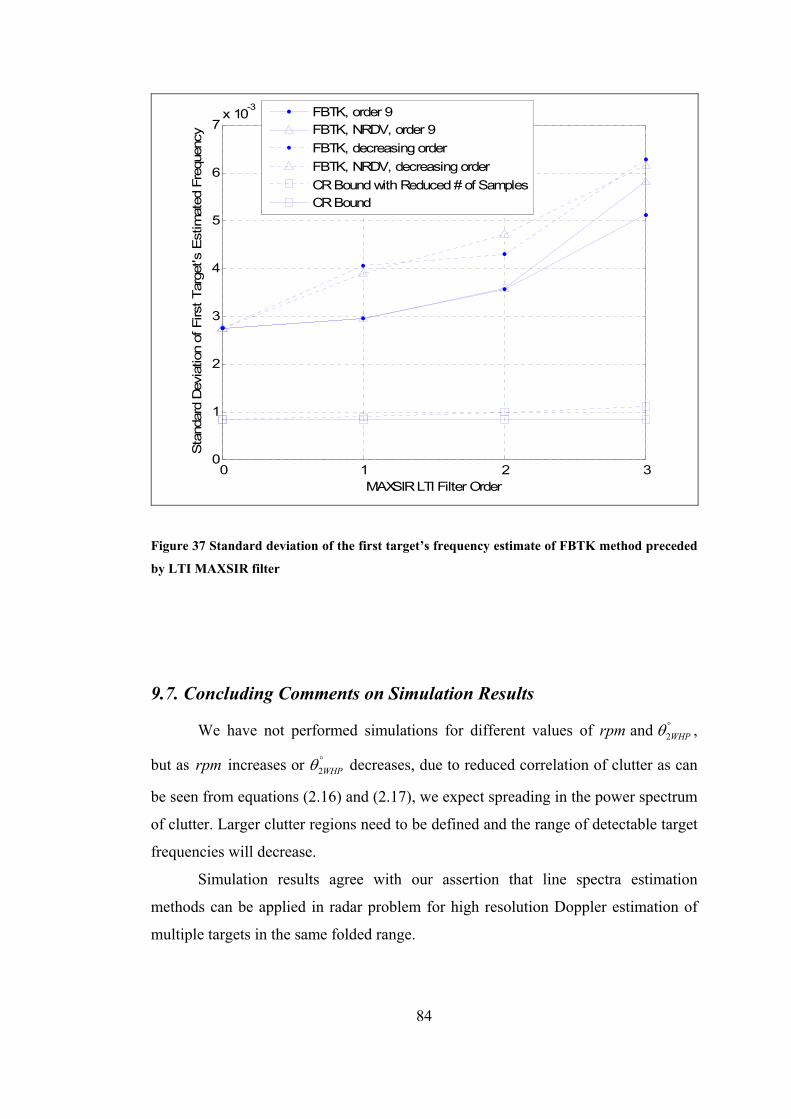
0 1 2 30
1
2
3
4
5
6
7x 10⁻³
MAXSIR LTI Filter Order
Sta
ndar
d D
evia
tion
of F
irst T
arge
t's E
stim
ated
Fre
quen
cy
FBTK, order 9FBTK, NRDV, order 9FBTK, decreasing orderFBTK, NRDV, decreasing orderCR Bound with Reduced # of SamplesCR Bound
Figure 37 Standard deviation of the first target’s frequency estimate of FBTK method preceded
by LTI MAXSIR filter
9.7. Concluding Comments on Simulation Results
We have not performed simulations for different values of ,
but as increases or decreases, due to reduced correlation of clutter as can
be seen from equations
2 and WHPrpm θ °
rpm 2WHPθ °
(2.16) and (2.17), we expect spreading in the power spectrum
of clutter. Larger clutter regions need to be defined and the range of detectable target
frequencies will decrease.
Simulation results agree with our assertion that line spectra estimation
methods can be applied in radar problem for high resolution Doppler estimation of
multiple targets in the same folded range.
84
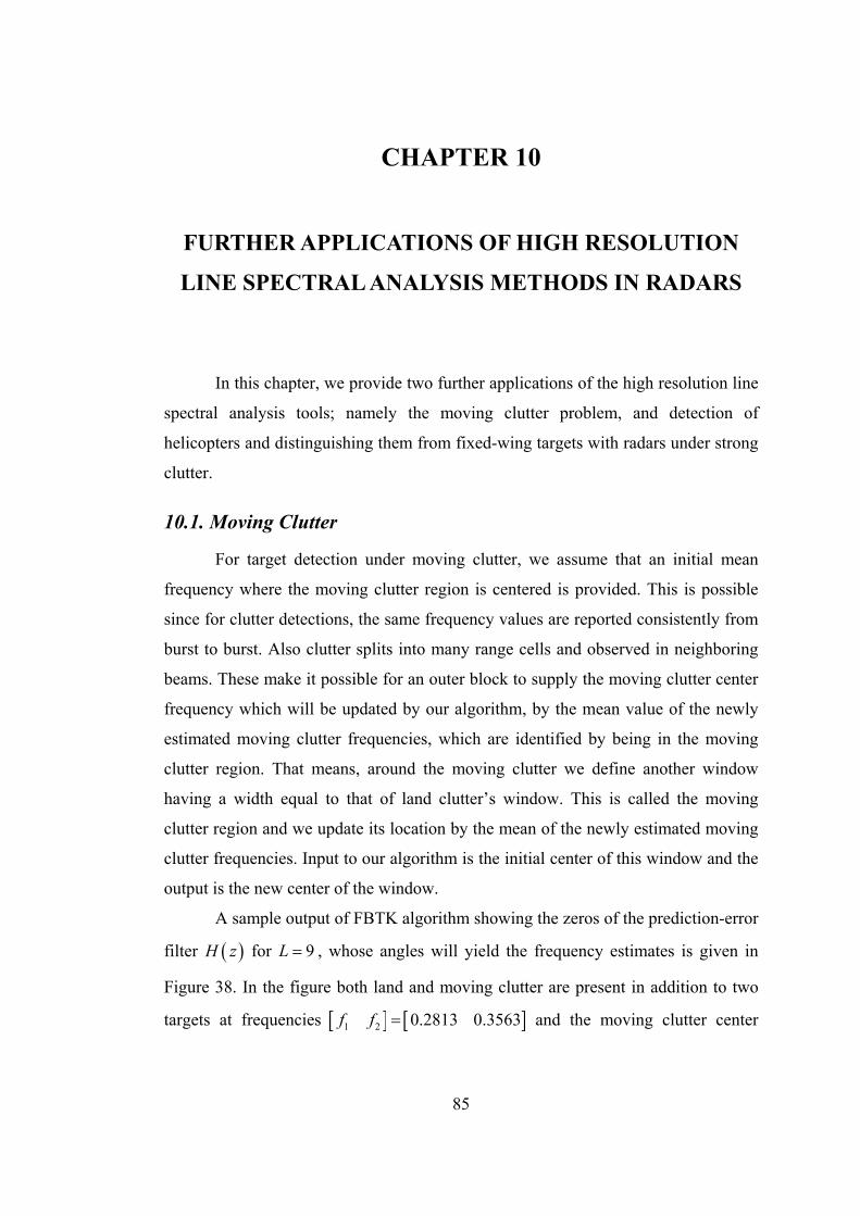
CHAPTER 10
FURTHER APPLICATIONS OF HIGH RESOLUTION
LINE SPECTRAL ANALYSIS METHODS IN RADARS
In this chapter, we provide two further applications of the high resolution line
spectral analysis tools; namely the moving clutter problem, and detection of
helicopters and distinguishing them from fixed-wing targets with radars under strong
clutter.
10.1. Moving Clutter
For target detection under moving clutter, we assume that an initial mean
frequency where the moving clutter region is centered is provided. This is possible
since for clutter detections, the same frequency values are reported consistently from
burst to burst. Also clutter splits into many range cells and observed in neighboring
beams. These make it possible for an outer block to supply the moving clutter center
frequency which will be updated by our algorithm, by the mean value of the newly
estimated moving clutter frequencies, which are identified by being in the moving
clutter region. That means, around the moving clutter we define another window
having a width equal to that of land clutter’s window. This is called the moving
clutter region and we update its location by the mean of the newly estimated moving
clutter frequencies. Input to our algorithm is the initial center of this window and the
output is the new center of the window.
A sample output of FBTK algorithm showing the zeros of the prediction-error
filter for , whose angles will yield the frequency estimates is given in ( )H z 9L =
Figure 38. In the figure both land and moving clutter are present in addition to two
targets at frequencies [ ] [ ]1 2 0.2813 0.3563f f = and the moving clutter center
85
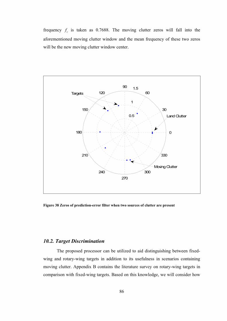
frequency cf is taken as 0.7688. The moving clutter zeros will fall into the
aforementioned moving clutter window and the mean frequency of these two zeros
will be the new moving clutter window center.
0.5
1
1.5
30
210
60
240
90
270
120
300
150
330
180 0
Land Clutter
Targets
Moving Clutter
Figure 38 Zeros of prediction-error filter when two sources of clutter are present
10.2. Target Discrimination
The proposed processor can be utilized to aid distinguishing between fixed-
wing and rotary-wing targets in addition to its usefulness in scenarios containing
moving clutter. Appendix B contains the literature survey on rotary-wing targets in
comparison with fixed-wing targets. Based on this knowledge, we will consider how
86
high resolution line spectra estimation algorithms can be employed for target
classification purposes after presenting the mathematical model for helicopters
(rotary-wing targets).
10.2.1. Modeling Helicopter Echo
The hub echo is assumed to be zero mean, Gaussian distributed, and
independent from the rest of the signal model components. If target is a helicopter,
its hub’s autocorrelation matrix is given by
thi
( )2
2 2, 2 sincij fhel hub hub
k lbody
fePRF
πσσ
⎛= ⎜⎝ ⎠
R k l ⎞− ⎟ (10.1)
which is used to model the helicopter hub echo h after defining the eigenvectors and
eigenvalues of as helR
( )Hhel hel hel hel=R V D V . (10.2)
( )1
2hel hel=h V D w (10.3)
where is an element column vector of complex white Gaussian noise. w N
In obtaining the CR bound for the rotary-wing target case, one just needs to
add the appropriate matrices to and use the resultant matrix as the new
in equations
helR nR nR
(3.22) - (3.27).
10.2.2. Proposed Classification Method
Line component estimation methods may be affected by the presence of the
hub echo, so, further investigation is required for this point. If we assume that the
effect is negligible and subtract the estimated body echoes from the received signal,
one can observe that helicopter and fixed-wing targets separate out. One can check
for the presence of a helicopter from the presence or absence of spreading. The
remaining power around the body frequency of a rotary-wing target after subtraction
may be either modeling the hub echo or may be present due to the imperfect
cancellation of the actual and estimated echoes, which is again due to the presence of
hub echo. In any case, classification capability of line component frequency
estimation methods seems promising to further investigate.
87
CHAPTER 11
CONCLUSION AND FUTURE WORKS
A radar detector and Doppler processor block based on linear prediction,
capable of operating under multiple-target and more than one source of clutter
scenarios has been investigated. A model order detector has been suggested with its
performance observed through simulations. Various simulation results on linear
prediction parameters and comparison of linear prediction, MUSIC, and ESPRIT
were given with results compared to the derived Cramér-Rao bounds. The effect of
using LTI maximizing filter prior to linear prediction was analyzed. How to use
the specified radar processor for target classification has been briefly explained.
SIR
The main result of this work is that linear prediction and high resolution line
spectra algorithms should be used in their forward-backward and nonwhitened
versions treating each source of clutter as a group of targets with close Doppler
frequencies. Other key results are:
1. Estimates obtained from the high resolution line spectra estimation
algorithms can be further improved with subsequent Maximum Likelihood
processing in order to obtain lower standard deviations and biases for the estimates.
2. Frequency estimates found by linear prediction cannot be improved with
preprocessing the data with a whitening filter or an MAXSIR filter.
3. There is an optimum order L for the prediction-error filter used in Tufts-
Kumaresan method, which is different than 3 4N found in the literature [1].
4. If one increases the number of samples N available to process, the order
of the prediction-error filter should be chosen accordingly. An initial increase in
may lower standard deviations of the estimates; however, further increase may
deteriorate the quality of the estimates.
L
L
88
5. All the frequency estimation algorithms examined show similar results
under varying , although Tufts-Kumaresan method produces the best estimates. SNR
6. High resolution line spectra estimation algorithms are affected from a
nearby clutter source or a target with a close frequency in the same way. This is
observed in the increase of the standard deviations and biases of the estimates.
However; Cramér-Rao bound increases only when there is a nearby clutter source.
7. For the model we used, it is expected that results obtained using land
clutter will not change if one has data corrupted with moving clutter since the only
difference in their models is the center frequency of the clutter.
8. It is expected that multiple clutter sources would be treated similarly by the
high resolution line spectra estimation algorithms since these algorithms do not
differentiate between clutter and the targets. It is the duty of the clutter region to
perform the necessary separation of targets and the clutter.
9. The proposed model order detector based on making threshold comparison
of the estimated amplitudes is successful at providing the total number of targets plus
clutter components.
10. A model order detector based on the closeness of the zeros of the
prediction-error filter to the unit circle does not provide promising results although it
will be probably beneficial to develop a model order determiner that takes as inputs
to it both the amplitude of the estimates and the closeness of the corresponding zeros
of the prediction-error filter to the unit circle.
11. Clutter region concept works well in separating targets from clutter. In
fact, with this concept we achieve a form of whitening since clutter components
which cause the noise part of the observation vector x to be colored is eliminated
with this operation.
As a future work, the number of target plus clutter components detection
procedure can be improved and a recently published modification on TK method
[37] can be adapted. Research can be conducted on the applicability of the
algorithms under clutter conditions that are modeled differently. Also target
classification procedure can be detailed and the computational complexity of the
algorithms can be investigated. Lastly, we anticipate that performance evaluation of
89

90
the algorithms on actual radar data can provide numerous insights and the methods
can be improved accordingly.
REFERENCES
[1] Tufts, D. W. and Kumaresan, R., “Estimation of Frequencies of Multiple Sinusoids: Making Linear Prediction Perform Like Maximum Likelihood,” IEEE Proceedings, vol. 70, no. 9, September 1982.
[2] Öztan, B. B. and Tanık, Y., “Estimation of the Parameters of Complex Exponentials under Radar Land Clutter and Single Snapshot Observation Using Modified Forward Backward Linear Prediction,” IEEE Sinyal İşleme, İletişim ve Uygulamaları Kurultayı, 2008.
[3] Richards, M. A., Fundamentals of Radar Signal Processing, McGraw-Hill, 2005.
[4] Skolnik, M. I., Introduction to RADAR Systems 3rd Ed., McGraw-Hill, 2001.
[5] Banjanin, Z., Zrnic’, D. S. and Cruz, J. R., “A Linear Prediction Approach to Doppler Mean Frequency Retrieval in the Presence of Ground Clutter,” IEEE Trans. on Aerospace and Electronic Systems, vol. 29, no. 3, July 1993.
[6] Nathanson, F. E., Reilly, J. P. and Cohen, M. N., Radar Design Principles Signal Processing and the Environment 2nd Ed., McGraw-Hill, 1991.
[7] D’addio, E., Farina, A. and Studer, F. A., “Performance Comparison of Optimum and Conventional MTI and Doppler Processors,” IEEE Trans. on Aerospace and Electronic Systems, vol. AES-20, no. 6, November 1984.
[8] Farina, A. and Protopapa, A., “New Results on Linear Prediction for Clutter Cancellation,” IEEE Trans. on Aerospace and Electronic Systems, vol. 24, no. 3, May 1988.
[9] Armstrong, B. C., “A Comparison of Conventional, Adaptive and Hybrid Doppler Processing Techniques,” Proc. South African Symposium on Communications and Signal Processing, 1992, pp. 127-134.
91
[10] Kay, S. M., Modern Spectral Estimation: Theory and Application, Prentice Hall, 1988.
[11] Therrien, C. W., Discrete Random Signals and Statistical Signal Processing, Prentice Hall, 1992.
[12] Hayes, M. H., Statistical Digital Signal Processing and Modeling, John Wiley & Sons, Inc., 1996.
[13] Rife, D. C., “Single-Tone Parameter Estimation from Discrete-Time Observations” IEEE Trans. On Information Theory, vol. IT-20, no. 5, September 1974.
[14] Rife, D. C. and Boorstyn, R. R., “Multiple Tone Parameter Estimation from Discrete-Time Observations” The Bell System Technical Journal, vol. 55, no. 9, November 1976.
[15] Van Trees, H. L., Detection, Estimation, and Modulation Theory Part I Detection, Estimation, and Linear Modulation Theory, John Wiley & Sons, Inc., 1968.
[16] Haykin, S., Currie, B. W. and Kesler, S. B., “Maximum-Entropy Spectral Analysis of Radar Clutter,” Proc. IEEE, vol. 70, no. 9, September 1982.
[17] Tufts, D. W. and Kumaresan, R., “Singular Value Decomposition and Improved Frequency Estimation Using Linear Prediction,” IEEE Trans. on Acoustics, Speech, and Signal Processing, vol. ASSP-30, no. 4, August 1982.
[18] Kumaresan, R., “On the Zeros of the Linear Prediction-Error Filter for Deterministic Signals,” IEEE Trans. on Acoustics, Speech, and Signal Processing, vol. ASSP-31, no. 1, February 1983.
[19] California Institute of Technology, “The Moore-Penrose Pseudo Inverse,” http://robotics.caltech.edu/~jwb/courses/ME115/handouts/pseudo.pdf, last date accessed: 30.06.2008.
92
[20] Koç, A. T., “Direction Finding With a Uniform Circular Array Via Single Snapshot Processing,” Ph.D. thesis, Middle East Technical University, Ankara, Turkey, 1996.
[21] Koç, A. T. and Tanık, Y., “Direction Finding With a Uniform Circular Array Via Single Snapshot Processing,” Elsevier Signal Processing 56, 1997, 17-31.
[22] Kumaresan, R. and Tufts, D. W., “Estimating the Parameters of Exponentially Damped Sinusoids and Pole-Zero Modeling in Noise,” IEEE Trans. on Acoustics, Speech, and Signal Processing, vol. ASSP-30, no. 6, December 1982.
[23] Khan, R. H., “Ocean-Clutter Model for High-Frequency Radar,” IEEE Journal of Oceanic Engineering, vol. 16, no. 2, April 1991.
[24] Olkin, J. A., Nowlin, W. C. and Barnum, J. R. “Detection of Ships Using OTH Radar with Short Integration Times,” Proc. IEEE National Radar Conf., Syracuse, USA, May 1997, pp. 1-6.
[25] Wax, M. and Kailath, T., “Detection of Signals by Information Theoretic Criteria,” IEEE Trans. on Acoustics, Speech, and Signal Processing, vol. ASSP-33, no. 2, April 1985.
[26] Oppenheim, A. V. and Schafer, R. W., Discrete-Time Signal Processing 2nd Edition, Prentice Hall, 1999.
[27] Ren, Q. S. and Willis, A. J., “Extending Music to Single Snapshot and On Line Direction Finding Applications,” IEE Radar 97, no. 449, October 1997.
[28] Xie, J., Yuan, Y. and Liu, Y., “Super-Resolution Processing for HF Surface Wave Radar Based on Pre-Whitened MUSIC,” IEEE Journal on Oceanic Engineering, vol. 23, no. 4, October 1998.
[29] Vaitkus, P. J., Cobbold, R. S. C. and Johnston, K. W., “A New Time-Domain Narrowband Velocity Estimation Technique for Doppler Ultrasound Flow Imaging. Part II: Comparative Performance Assessment,” IEEE Trans. on Ultrasonics, Ferroelectrics, and Frequency Control, vol. 45, no. 4, July 1998.
93
[30] Ivkovic, D. S., Simic, S., Dukic, M. L. and Eric, M. M., “Software Model of the Signal Processing Unit in the Conventional Radar,” IEEE EUROCON, November 2005.
[31] Wang, J. and Kirlin, R. L., “Improvement of High Frequency Ocean Surveillance Radar Using Subspace Methods Based on Sea Clutter Suppression,” Proc. Sensor Array and Multichannel Signal Processing Workshop, August 2002, pp. 557-560.
[32] Shahapurkar, N. and Ramalingam, C. S., “Threshold Performance of MUSIC When Using the Forward-Backward Data Matrix,” IEEE Signal Proc. Letters, vol. 13, no. 2, February 2006.
[33] Shah, A. A. and Tufts, D. W., “Determination of the Dimension of a Signal Subspace from Short Data Records,” IEEE Trans. on Signal Processing, vol. 42, no. 9, September 1994.
[34] Wildman, P., “STAT 2005 Homepage Chapter 6 Lessons,” http://wind.cc.whecn.edu/~pwildman/statnew/chapter_6_lessons.htm, Casper College, Spring 2002, last date accessed: 27.06.2008.
[35] McGraw-Hill, Confidence Intervals and Sample Size, http://highered.mcgraw-hill.com/sites/dl/free/0072549076/79745/ch07.pdf, May 2003, last date accessed: 27.06.2008.
[36] Maddock, J., Bristow, P. A., Holin, H. and Zhang, X., “boost Math Toolkit,” http://freespace.virgin.net/boost.regex/toolkit/html/index.html, September 2007, last date accessed: 27.06.2008.
[37] So, H.-C. and Leung, C.-T., “A Simple Improvement to Tufts-Kumaresan Method for Multiple Sinusoidal Frequency Estimation,” IEICE Trans. Fundamentals, vol. E88-A, no. 1, January 2005.
[38] Proakis, J. G., Digital Communications 4th Edition, McGraw-Hill, 2001.
[39] Wikipedia The Free Encyclopedia, “Newton’s Method in Optimization,” http://en.wikipedia.org/wiki/Newton%27s_method_in_optimization, May 2008, last date accessed: 28.06.2008.
94
[40] Tikkinen, J. M., Helander, E. E., and Visa, A., “Joint Utilization of Incoherently and Coherently Integrated Radar Signal in Helicopter Categorization,” IEEE, 0-7803-8882-8/05, 2005.
[41] Feng X., Yan J., Huang P., and Xiao Z., “Detection of Hovering Helicopter,” ICSP’02 Proceedings, 0-7803-7488-6/02, IEEE 2002.
[42] Yoon, S.-H., Kim, B., and Kim, Y.-S., “Helicopter Classification Using Time-Frequency Analysis,” Electronics Letters, vol. 36, no. 22, 26th October 2000.
[43] Ziyue T., Yongliang W., and Zhiwen W., “STAP Scheme to Detection of Hovering Helicopter,” Proceedings of ICSP2000, 0-7803-5747-7/00, IEEE 2000.
[44] Gini, F. and Farina, A., “Matched Subspace CFAR Detection of Hovering Helicopters,” IEEE Trans. Aerospace and Electronic Systems, vol. 35, no. 4, October 1999.
[45] Kulpa, K., Czekala, Z., Misiurewicz, J., and Falkiewicz, J., “Parametric Detection of the Helicopter Hub Echo,” IEEE, 0-7803-4977-6/99, 1999.
[46] Rotander, C E and Sydow, H von, “Classification of Helicopters by the L/N-Quoutient,” IEE, Radar 97, Publication No. 449, 14 – 16 October 1997.
[47] Misiurewicz, J., Kulpa, K., and Czekala, Z., “Analysis of Recorded Helicopter Echo,” IEE, Radar 97, Publication No. 449, 14 – 16 October 1997.
[48] Bullard, B. D. and Dowdy, P. C., “Pulse Doppler Signature of a Rotary-Wing Aircraft,” IEEE, CH2952-0/91/0000-0160, 1991.
[49] Misiurewicz, J., Kulpa, K., and Czekala, Z., “Analysis of Radar Echo from a Helicopter Rotor Hub,” Warsaw, Poland.
[50] Abatzoglou, “Helicopter Recognition Radar Processor,” United States Patent, No.: US 7,079,072 B1, Date: Jul. 18, 2006.
95
96
[51] Nagel, “Radar Process for Classifying or Identifying Helicopters,” United States Patent, No.: US 7,046,192 B2, Date: May 16, 2006.
[52] Hommel et al., “Target Classification Method,” United States Patent, No.: US 6,573,861 B1, Date: Jun. 3, 2003.
[53] Shi et al., “Radar Detection and Classification of Helicopters,” United States Patent, No.: 5,689,268, Date: Nov. 18, 1997.
[54] Abatzoglou, “Helicopter Recognition Radar Processor,” United States Patent, No.: 5,376,940, Date: Dec. 27, 1994.
[55] Ludloff et al., “Method for Detecting and Classifying Helicopters,” United States Patent, No.: 5,231,402, Date: Jul. 27, 1993.
APPENDIX A
IMPLEMENTATION OF MAXIMUM LIKELIHOOD
TECHNIQUE
Equations (3.9) and (3.10) can be solved using the steepest descent method
[38] in which case the specified equations without equating to zero provide the
necessary gradient information. If one uses an algorithm that requires real variables,
entries of the gradient are given by
( )( ) { } { }( )
( ) { } { }( ) { } { }
:, :, :,1
:, :, :,1
* ' ':, :, :,1
ln2Re 2Re , 1, ,
ln2Re 2Re , 1, ,
ln2Re 2Re , 1, ,
MH Hk k l ll
k real
MH Hk k l ll
k imaginary
M H Hi p i p p pi
p
pa k M
a
pj j a k
a
pa a a p M
ω
=
=
=
∂= − + =
∂
∂= + − =
∂
∂= −
∂
∑
∑
∑
V Qx V Q V
V Qx V Q V
V QV x QV
…
…
…
M
=
.(A.1)
In the steepest descent algorithm, estimates for any generic variable z is updated as
( )ln
old
new oldz z
pz z
zμ
=
∂= −
∂ (A.2)
where μ is a properly chosen step size parameter that should guarantee convergence.
Another possibility may be to use Newton–Raphson method [39] with the
update equation
(A.3) ( ) ( ) ( ) (1
ln lnnew old old oldp pγ−
⎡ ⎤= − ∇⎣ ⎦z z H z z )
which requires the Hessian matrix in addition to gradient information ( )ln pH ( )ln p∇ .
is the matrix of second-order partial derivatives of the cost function ( )ln pH ( )ln p (−
sign is omitted for short notation) with the ( element given by )th,i j [12]
97
( ) ( ){ } ( )( )2
ln ,
lnp i j
i j
p∂=
∂ ∂
zH z
z z. (A.4)
The necessary equations corresponding to our model required to form the Hessian
matrix are
( )
( ) { } { }( ) ( ){ }( ) ( ) ( )( )
2
:, :,
2'' * ''
:, :, :,2 1
2* ' '
:, :,
2' ' '
:, :, :, :, :,1
2'
:, :,
ln
ln2 Re 2 Re
ln2 Re , valid for
ln
ln,
Hk t
k t
MH Hk k l k l kl
k
H
t k t kk t
HH MHk k k k l kl
k k
Hk t k
k t
pa a
pa a a
pa a k t
pa a
a
pa
a
ω
ω ω
ω
ω
=
=
∂=
∂ ∂
∂= − +
∂
∂= ≠
∂ ∂
∂= − + +
∂ ∂
∂=
∂ ∂
∑
∑
V QV
x QV V QV
V QV
V Qx V QV V QV
V QV valid for k t≠
l
⎤⎦
(A.5)
where is '':,kV
. (A.6) ( ) ( )2 1'':, 0 1 pk
Tj Njk e N e ωω −⎡= − − −⎣V
If one requires the corresponding equations for algorithms accepting real variables,
they are given as
( )( ) ( ) { }
( )( ) ( ) { }
( )( ) ( ) { }
( ) { } { }( ) ( ){ }
2
:, :,
2
:, :,
2
:, :,
2'' * ''
:, :, :,2 1
2* ' '
:, :,
ln2 Re
ln2 Re
ln2 Re
ln2 Re 2 Re
ln2 Re ,
Hk p
k preal real
Hk p
k pimaginary imaginary
Hk p
k preal imaginary
MH Hk k l k l kl
k
H
p k p kk p
pa a
pa a
pj
a a
pa a a
pa a
ω
ω ω
=
∂=
∂ ∂
∂=
∂ ∂
∂=
∂ ∂
∂= − +
∂
∂=
∂ ∂
∑
V QV
V QV
V QV
x QV V QV
V QV
( )( ) ( ){ } ( ) { } ( ){ }
2' '
:, :, :, :, :,
valid for
ln2 Re 4 Re 2 Re
H HHk k k k kreal
k k real
k p
pa a
aω
≠
∂= − + +
∂ ∂V Qx V QV V Q V'
k k
98
( )( ) { }
( )( ) ( ){ } ( ) { }
( ){ }( )
( ) { }
2'
:, :,
2' '
:, :, :,
':, :,
2'
:, :,
ln2Re , valid for
ln2Re 4 Re
2Re
ln2Re , valid for
Hk p k
k p real
H Hk k k kimaginary
k k imaginary
H
k k k
Hk p k
k p imaginary
pa k p
a
pj a
a
j a
pja k p
a
ω
ω
ω
∂= ≠
∂ ∂
∂= +
∂ ∂
−
∂= − ≠
∂ ∂
V QV
V Qx V QV
V Q V
V QV
+. (A.7)
What we have used in solving the minimization problem (3.6) is the
MATLAB function fminunc with gradient and Hessian information provided by us.
Another alternative we tried is to minimize equation (3.18) without providing
gradient or Hessian information to the same MATLAB function. One can refer to
MATLAB help for further details.
99
APPENDIX B
LITERATURE ON HELICOPTER ECHO AND
DETECTION AND CLASSIFICATION
In this part, a summary of the references [40] - [55] will be presented. If
and time-on-target ( values are appropriately selected, helicopter radar echo
possesses some characteristic features. Additionally, PRF , which is the data
sampling rate for a pulse Doppler radar, must be high enough (10s of kHz) for
representing the helicopter echo without aliasing (an unambiguous velocity of at least
500 m/s is necessary). Helicopter backscattering results from several reflectors
including fuselage, main rotor blades, tail rotor, rotor hub, and reflections caused by
the interaction & interference of these components etc.
SNR
)N PRIi
B.1. Body (Fuselage, Skin)
Fuselage echo resembles that of a fixed-wing aircraft with radar cross-section
( RCS ) of a few square meters (Note that RCS changes with radar frequency and
target orientation). Since rotary-wing targets have other components contributing to
the echo signal, spectral width of their echoes are expected to be larger than those of
fixed-wing targets. Fuselage echo may overlap with the spectrum of clutter in the
case of hovering; otherwise, it has a Doppler frequency depending on radial velocity
relative to the radar. The effect of undesired ground clutter is not present when the
helicopter is not a hovering one.
B.2. Main Rotor
The main rotor consists of several blades rotating at a rate of 200 ~ 350 rpm.
The rotation speed of the main rotor remains nearly constant during the flight and the
maximum velocity of the tips of the main rotor blades varies only slightly between
100
different types of helicopters (blade end linear velocity is about 180 – 230 m/s). The
approaching tip of the main rotor blade has the highest velocity component, whereas
it is the opposite for the receding tip of the main rotor blade.
The echo of the periodically rotating blades of the main rotor consists of
successive intense temporal flashes (caused when consecutive rotor blades are
perpendicular to the direction of radar beam yielding the maximum RCS ) with
evenly distributed two-sided Doppler signature around the fuselage line (both
amplitude and phase modulation are caused in radar echo). For even number of rotor
blades, the spectrum will be symmetrical since the backscattered signals of coming
and going blades will be simultaneous. For the odd number case with short
integration times the spectrum is slightly asymmetrical. Flash duration depends on
the length of the blades, rotor rate, and radar wavelength, while the flash interval
depends on the rotor rate and the rotor blade number. Power reflected by the blades
is typically less than 1% of the total reflected power.
At X-band 230m/s rotor tip speed results in approximately 15 kHz of Doppler
shift, indicating a minimum sampling rate of 30 kHz. Maximum forward flight
speeds of helicopters are limited approximately to 100 m/s due to retreating blade
stall. Consequently, maximum Doppler shift of an advancing blade tip of a helicopter
in forward flight can increase up to 22 kHz necessitating a minimum radar PRF of
44 kHz.
PRF
Since echo components of main and tail rotors are distributed over a broad
spectral range, for the cases when Doppler filter bank is employed, one may
sometimes observe that output signals from majority of the individual filters (> 75%)
are above the threshold. Neglecting those corresponding to the fuselage, outputs that
are above the threshold exhibit very little amplitude spread indicating presence of a
helicopter.
Rotor blade echo consisting of very short spikes is not very promising for a
surveillance radar since it may go unnoticed as common time-on-target values are
much smaller than spike repetition rate. In other words integration time long enough
for registering two or more successive main rotor flashes is required. As a rule of
thumb 100s of ms to a second of observation time is required to detect the rotor blade
flashes successfully. Helicopter classification can be based on an estimate of the
101
quotient of the number of rotor blades and their length; however, this requires high
or Signal to Clutter Ratio ( SC ). SNR R
B.3. Tail Rotor
The tail rotor has smaller diameter and higher rotation rate (50 – 110 rps). Its
echo also consists of spikes, but the spikes are smaller and more frequent. The echo
of the tail rotor remains often invisible because of being hidden by the fuselage. If
horizontal polarization is used in transmission and reception, effect of modulation
caused by the vertically rotating tail rotor can be neglected in the received signal.
B.4. Hub
Hub is the mechanical joint that serves many functions in addition to
connecting the blades to the engine shaft: power transfer, blade attack angle steering,
and damping of blade vibrations to name a few. The origin of the triangular shaped
spectral area centered on the fuselage line component is the hub. At X-band it
occupies a ±2 kHz bandwidth (considering 99% power). The RCS of the hub is in
the range of 0.25 m2, lower than the fuselage echo by 5 – 20 dB. Taking hub return
power equal to one tenth of target skin return is a feasible approach. Since the RCS
of the hub of a helicopter is very small, a technique based on using the echoes of hub
is feasible for a helicopter target in close range which is actually what we are
interested in. Hub detection is also suitable for the scenarios with relatively short
time-on-target values (10s of ms). In fact spectral signature of the rotor hub has a
higher probability of occurrence than the blade flash.
Analyzed portion of the signal should contain no spikes, namely, the rotor
flashes, as it would interfere with the detection of a helicopter based on its hub
spectrum.
In determining the radar echo strength the transmitted power is multiplied by
the square of the radar antenna pattern for mechanically scanned antennas in the time
domain. This is equivalent to convolution operation in the frequency domain which,
therefore, widens the fuselage spectrum covering the weak hub echo. The use of
further time windowing lowers the frequency resolution more. Taking into account
the typical width of the hub spectrum for different wavelengths, the Fourier analysis
102
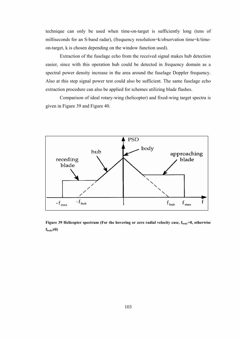
technique can only be used when time-on-target is sufficiently long (tens of
milliseconds for an S-band radar), (frequency resolution=k/observation time=k/time-
on-target, k is chosen depending on the window function used).
Extraction of the fuselage echo from the received signal makes hub detection
easier, since with this operation hub could be detected in frequency domain as a
spectral power density increase in the area around the fuselage Doppler frequency.
Also at this step signal power test could also be sufficient. The same fuselage echo
extraction procedure can also be applied for schemes utilizing blade flashes.
Comparison of ideal rotary-wing (helicopter) and fixed-wing target spectra is
given in Figure 39 and Figure 40.
Figure 39 Helicopter spectrum (For the hovering or zero radial velocity case, fbody=0, otherwise
fbody≠0)
103
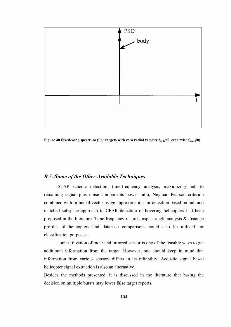
Figure 40 Fixed-wing spectrum (For targets with zero radial velocity fbody=0, otherwise fbody≠0)
B.5. Some of the Other Available Techniques
STAP scheme detection, time-frequency analysis, maximizing hub to
remaining signal plus noise components power ratio, Neyman–Pearson criterion
combined with principal vector usage approximation for detection based on hub and
matched subspace approach to CFAR detection of hovering helicopters had been
proposed in the literature. Time-frequency records, aspect angle analysis & distance
profiles of helicopters and database comparisons could also be utilized for
classification purposes.
Joint utilization of radar and infrared sensor is one of the feasible ways to get
additional information from the target. However, one should keep in mind that
information from various sensors differs in its reliability. Acoustic signal based
helicopter signal extraction is also an alternative.
Besides the methods presented, it is discussed in the literature that basing the
decision on multiple bursts may lower false target reports.
104