Linear Models and Sequential Hypothesis Testingmath.ucsd.edu/_files/undergraduate/honors-program/honors-program... · This is an expository paper on FDR control of sequential hypotheses,

Linear Models and Sequential HypothesisTesting

Drew T. Nguyen

Abstract. This is an expository paper on FDR control of sequentialhypotheses, with application to model selection in linear models with or-thogonal design. We state the problem and outline, from start to finish,a complete method to perform model selection—including variations,recommendations, and some discussion of historical and current meth-ods. Detailed proofs are provided for all main results and some of theimportant tools. In particular, the author proposes the use of a lesser-known test statistic, robust to nonorthogonality, and demonstrates itsefficacy compared to a standard method.

Contents

Acknowledgements and Dedication 21. Introduction 22. Model Selection 33. The Lasso and p-values for Model Selection 54. Multiple Hypothesis Testing and the FDR 125. Continuous-time Martingales and the Optional Stopping Theorem 136. The Benjamini-Hochberg procedure 167. Sequential Hypothesis Testing 208. ForwardStop 229. Accumulation test procedures, SeqStep, and HingeExp 2610. Simulation results 3411. Discussion and Conclusion 3512. References 38

1

2 DREW T. NGUYEN

Acknowledgements and DedicationThis is my undergraduate honors thesis in mathematics at UCSD, sub-

mitted in March 2018.I would like to thank my parents, who would have liked me to be back

home, but who supported my decision to go on working on projects at UCSDa little while longer; my brother, always a pillar of support; my thesis ad-visor Ian Abramson, whose floral lectures and dreamy attitude for statisticsshaped my interest over the last several years; Jelena Bradic, whose class onstatistical learning first got me into these problems; Ery Arias-Castro, whoseoccasional conversations helped me sharpen my understanding on my thesistopic in particular; Kenshi Yonezu and REOL, whose music got me throughthe winter I wrote it; and all the folks at NanoDesu Translations, for beingsuch great friends, and missing me while I was gone. Sorry, guys, I havebeen a bit MIA. This is done now, though, so I’ll see you again soon.

I dedicate this work to Madoka Kaname, who is an inspiration to us all.

1. IntroductionThis work is motivated by the model selection problem in the usual linear

regression setup with iid Gaussian error:y = X�⇤

+ ✏ (1)where y 2 Rn,X 2 Rn⇥p,�⇤ 2 Rp, ✏ ⇠ Nn(0,�

2I).Suppose we have a candidate estimate for the vector �⇤; call it ˆ�. Model

selection (and its cousin variable selection) attempt to answer the problemof how to pick ˆ� such that it has nonzero entries where �⇤ does, and zeroentries where �⇤ does; a choice of nonzero ˆ�i’s is called a model, and if a ˆ�iis nonzero we say it is included in the model.

One way to approach the problem is by considering an ordered sequence ofmodels, constructed by some mechanism (to be specified): M

1

,M2

, ...,MN

for some N , where each model Mk ✓ {1, ..., p} indexes the included �i’s.Given this sequence of models, how do we decide which Mk to settle on?

Different approaches exist. One method is to associate each with a certainscore function, and select the one that ranks highest (the score used is oftenthe BIC score). Another method is to use cross-validation.

For the sake of this work, we will pursue a method based on sequentialrejection of hypotheses, which, unlike the methods based on scores, give usprobabilistic guarantees. This means that we will treat the Mk in order,using hypotheses for each that tests whether Mk is “right”, per the modelselection problem.

Specifically, we consider the hypothesesH

0k : supp(�⇤) ✓ Mk, H

1k : supp(�⇤) 6✓ Mk (2)

where supp(�⇤) ✓ {1, ..., p} denotes those true nonzero indices of the model.

Though once again we note that even here there are alternatives; there are

LINEAR MODELS AND SEQUENTIAL HYPOTHESIS TESTING 3

different hypotheses one could use to quantify this idea of testing for the“right” Mk, and they are not equivalent. We will discuss these at the end.

There are two parts to this method, and so the present work is modular,also in roughly two parts, plus some space for background material. One partis the problem of generating p-values corresponding to each of the hypothe-ses H

0k, this is section 2 and 3. The second part, which is all subsequentsections, is to combine these p-values in a sensible way to select a modelwhile respecting multiple testing concerns.

First, in section 2 we begin by discussing difficulties involved in generatingp-values, and then in section 3 describe an established method that workscalled the covariance test. Also in section 3 we pursue a suggestion by T.Tony Cai and Ming Yuan, and propose a second method which is more robustto inexact assumptions; Cai and Yuan did not provide a proof, but we provideit here. Second, we develop some background material in sections 4, 5, and6, and then go into sequential hypothesis testing in sections 7, 8, and 9.That is, we consider p-values as generated from some distribution and forgetabout the calculation that produced them, and consider rejecting hypothesesin sequence using these p-values. The goal is to control an analogue of type-Ierror, called the FDR. Lastly, in section 10 we combine the p-values fromgenerated from the first part using the techniques from the second part andcompare performance between the covariance test and the proposed newstatistic.

So as not to detract from the main points—namely p-value generationand FDR control—we will necessarily not prove everything. As far as factsnot taught in yearly undergrad or graduate courses at UCSD, we’ll use somebasic properties of the lasso path, as well as some of the major theorems fromextreme value theory and continuous time martingale theory. The relevantresults require a lot of setup for their proofs, so much of that will be left to thereferences; in particular we will omit proofs for the needed standard resultson lasso properties [1] [2], and extreme distributions [3], in part because thoseresults can be simply stated, and we’ll sometimes refer to them casually inprose. We will also assume the standard martingale results from discretetime, but then prove the main theorem we need for continuous martingales,because even though it takes some setup, the language of martingales israther more technical and I find it illuminating to set them up in detail.

2. Model SelectionIn the linear model y = X�⇤

+ ✏, the p columns of X represent datacorresponding to p predictors, while the rows correspond to the n samples.For instance, math test scores may depend on socioeconomic factors for nstudents. We may have their test score (an entry of y) and collect n datarows with p entries (a row of X), such as family income, age of parents, orwhether they know a second language. In this case p = 3.

4 DREW T. NGUYEN

When fitting this model, we have to select which parameters to includeand so which data to keep. Maybe we fear that are our parents’ age aren’treally relevant (though in this hypothetical situation, it is). A researcher mayuse either domain knowledge or, more often, statistical techniques to selectcorrect parameters and thereby improve prediction and interpretability.

There are no shortage of statistical techniques for variable selection, butthere are shortcomings with some of the more obvious (i.e. naive) procedures.

Here is a first try. Suppose we wish to test the nulls H01

, ..., H0k, ..., H0p

that �k = 0 (from here I will simply write Hk for the kth null.) The Waldtest statistic is

ˆ�k

cs.e.h

ˆ�k

i

where ˆ�k is obtained by OLS and the denominator is an estimate of thestandard error (omitting here the exact formula). Under Hk, its distribu-tion is tn�(p+1)

, so to perform variable selection, you can start with all thevariables in the model, compute their p-values, and then leave out the vari-able with the largest p-value. Subsequently, you refit. This method is called“backwards selection”.

There is no theoretical problem with this—but only as long as you don’tascribe any theoretical properties to it. Certainly what this will do is it willgive us a sequence of variables �j

1

,�j2

, ...�jp to remove, but we cannot say weare doing valid hypothesis testing at each stage. After refitting, if we computep-values again, then the new p-values we obtain have been affected by ourselection of those variables and are thus invalid. In other words, the modelwe have selected and therefore the hypotheses we test have been influencedby our data. This is problematic, because we expect the hypotheses to bechosen beforehand.

Indeed, any procedure that reports p-values but does not account for thehypothesis having been selected based on the data is invalid. A procedurethat does account for this selection is called an adaptive procedure.

As noted in the introduction, one does not require valid p-values or adap-tive procedures to perform model selection. Backwards selection is still used,for instance, since it is a mechanism that gives us a sequence of models, andthe researcher can select the set of variables with the best BIC score, orpick one based on cross-validation. Other methods in use are forward step-wise (like backwards elimination, but adds variables), forward stagewise (likeforward stepwise, but more restrictive), and best subset regression.

These techniques remain controversial, however, because they do not givetheoretical guarantees (except for best subset regression, which is computa-tionally intractable for moderately sized datasets). But we can obtain someguarantees using adaptive procedures; in particular we can control how manytype-I errors are made, as long as a correct null distribution can be derived.


In section 3 we introduce the lasso estimator, from which an adaptiveprocedure for model selection can be derived.

3. The Lasso and p-values for Model SelectionThe lasso estimator is defined for the linear model (1) as the solution to

the following optimization problem:

ˆ�(�) := argmin

�

1

2

ky �X�k22

+ �k�k1

(3)

where one can think of � � 0 as enforcing a penalty to the objective functionbased on the size of the coefficients of �. This has the property that as� ! 1, every �i ! 0, while as � ! 0, ˆ�� ! ˆ�OLS , the ordinary leastsquares estimate.

For A ✓ {1, ..., p}, we will also soon use the following definition:

ˆ�A(�) := argmin

�

1

2

ky �XA�Ak22

+ �k�Ak1

(4)

where a subscript XA is the matrix X but only including those columnswhose indices are in A, and likewise �A includes only those entries from �.

In practice, variables �i both enter the model (go from zero to nonzero)and leave the model at finite values of �. These values of � are called knots,and we have 1 > �

1

� �2

� �3

� ... � �N , where �1

must be a knot wherea variable enters the model and N is bounded above by 3

p. If the columnsof X are in general position we have instead strict inequality, and the lassosolutions are unique [2]. If XTX = I, we say that X satisfies orthogonaldesign, or simply that X is orthogonal. In this case variables never leave themodel and N = p.

The lasso is used in high dimensional problems (p > n) because it is effi-ciently computable and has nice theoretical properties regarding consistencyand support recovery1, up to some technical conditions on X. For us, thelasso is nice because it provides valid p-values to judge the significance ofthe models that it selects.

The null distribution will turn out to be exact for orthogonal X, so weconsider this scenario2; then we have that N = p. Consider a knot �k. LetAk ✓ {1, ..., p} be the nonzero indices of � just before � = �k (this is calledthe active set) and suppose that at this knot the variable �ik enters themodel. Let supp(�⇤

) ✓ {1, ..., p} denote those true nonzero indices of themodel.

With the hypothesesH

0k : supp(�⇤) ✓ Ak, H

1k : supp(�⇤) 6✓ Ak (5)

1Support recovery means that for some �, the entries of ˆ�� are zero where �⇤, andtheir signs match when they are not, so that this � “recovers” the correct nonzero entriesand signs.

2Certainly this is a restrictive condition; we discuss it at the end.

6 DREW T. NGUYEN

we define the test statistic

Tk =

1

�2

⇣

hy,X ˆ�(�k+1

)i � hy,XAkˆ�Ak

(�k+1

)i⌘

(6)

which is the difference in the (uncentered) covariance of the response y andthe fitted values X� with the inactive data left in and left out, normalizedby the true variance. Tk is called the covariance test statistic.

Theorem 1 (Covariance Test). Under H0k and with XTX = I,

Tkd! Exp(1) (7)

as p ! 1, with n > p, and their p-values are independent.

Before proceeding with the proof, we need a lemma. We only state it:

Lemma 1. Under orthogonal design, Tk can be expressed in “knot form”:

Tk =

1

�2

· �k(�k � �k+1

) (8)

The proof of Lemma 1 starts from a closed form for the lasso estimatorˆ� given in [4] and proceeds through a (very) long chain of algebraic manip-ulations to obtain (8). The manipulations were done in great detail in theUCSD honors thesis [5] and we do not repeat them here.

We now use Lemma 1 and rewrite (8) into a form where the randomvariables involved are explicit. We will use a basic fact about the lasso,found in introductory sources such as [1]: Under orthogonal design, thelasso solution has the closed form

ˆ�j(�) = S�(ˆ�OLSj ) (9)

where S� : R ! R is the soft-thresholding function

S� =

8

>

<

>

:

x� � if x > �

0 if �� x �

x+ � if x < �

We note also that under orthogonal design ˆ�OLSj = XT

j y. Let Uj = XTj y.

Then the knots of the lasso are simply the values of � where the coefficientsbecome nonzero (cease to be thresholded):

�1

=

�

�U(1)

�

�,�2

=

�

�U(2)

�

�, ...,�p =�

�U(p)

�

� (10)

where�

�U(1)

�

� � �2

=

�

�U(2)

�

� � ... � �p =

�

�U(p)

�

� denote the order statisticsin reverse order of |U

1

|, ..., |Up|. This is a slight abuse of notation—they arenot the absolute values of the order statistics U

(1)

, ..., U(p).

Under the null hypothesis, the entries of the OLS estimate are iid N (0,�2

),so |Ui|/�2

iid⇠ |N (0, 1)|, and we write

Tk =

1

�2

�

�U(k)

�

� · ��U(k)

�

�� U(k+1)

�

�

�

(11)


Proof of the covariance test. Because in the orthogonal case, variablesnever leave the model and N = p, we have A

1

✓ A2

✓ ... ✓ Ap. Then as-suming the truth of the H

0k : supp(�⇤) ✓ Ak implies assuming the falsehood

of every H0k0 : supp(�⇤

) ✓ Ak0 for k0 < k. In other words, under H0k all

variables added to the model before step k are not null3 and the remainingknots

�

�U(k)

�

�, ...,�

�U(p)

�

� are the order statistics of the remaining |Ui|, so�

�U(k)

�

�

may be thought of as the maximum of them and�

�U(k�1)

�

� the second largest.Hence we need only show the result for T

1

=

�

�U(1)

�

� · ��U(1)

�

�� U(2)

�

�

� �

�2,which depends on a maximum and second largest order statistic, and theresult follows with the exact same proof for the other Tk. For a similarreason, the resulting p-values are independent; the distribution we derive forTk is conditional on the null being false for the k0 < k and true at k, whilethe Tk0 is conditional on the null being true at k0 < k, which are disjointevents. So the p-values pk are always independent of p

1

, ..., pk�1

. Then anyset of p-values pk

1

, ..., pkj is mutually independent because

P (pk1

x1

, ..., pkj xj) = P (pk1

x1

, ..., pkj�1

xj�1

)P (pkj xj)

= ... =

jY

i=1

P (pki xi)

Now we show the result for T1

. Each |Ui|/�2 has CDF

F (x) = (2�(x)� 1) {x > 0}We would like to know the distribution of its extreme order statistics

as p ! 1, and apply some basic extreme order statistics theory. Let Hdenote the left continuous inverse of 1/(1�F ). Then Theorem 1.1.8, Remark1.1.9, and Theorem 2.1.1. from de Haan and Ferreira (2006) [3] togetherimmediately imply that if

lim

t!1(1� F (t))F 00

(t)

F 0(t)2

= �(� + 1)

then for ap = H�1

(p) and bp = pF 0(ap), we have that W

1

= bp�

�

�U(1)

�

�� ap�

and W2

= bp�

�

�U(2)

�

�� ap�

converge jointly in distribution:

(W1

,W2

)

d!

E��1

� 1

�,(E

1

+ E2

)

�� 1

�

!

where if � = 0 the right hand side is interpreted as (� log(E1

),� log(E1

+

E2

)), which is its limit as � ! 0, and the E’s are iid Exp(1).

3Lockhart et al. assume some mild technical assumptions, but they don’t condition onthe first k0 variables entering being those in the true model, and prove a stronger result intheir Theorem 1 [6]. Since we’ll always be rejecting hypotheses sequentially (see section7), we won’t need to do this.

8 DREW T. NGUYEN

Indeed � = 0; we compute(1� F (t))F 00

(t)

F 0(t)2

=

F 00(t)

F 0(t)

1� F (t)

F 0(t)

=

�2t�(t)

2�(t)

2� 2�(t)

2�(t)= �t · 1� �(t)

�(t)

so that

lim

t!1(1� F (t))F 00

(t)

F 0(t)2

= lim

t!1�t · 1� �(t)

�(t)= lim

t!1�t ·m(t)

where m(t) is the Mills’ ratio (1 � �(t))�

�(t) for the standard normal, forwhich it’s well known that m(t) ⇠ 1/t for large t. So the limit is �1, implying� = 0 and

(W1

,W2

)

d! (� log(E1

),� log(E1

+ E2

))

Note that�

�U(1)

�

� · ��U(1)

�

�� U(2)

�

�

�

= (ap +W1

/bp)(W1

�W2

)

1

bp

=

apbp

(W1

�W2

) +

W1

(W1

�W2

)

bp

Now, writing explicitly ap and bp, we have ap = F�1

(1�1/p) = �

�1

(1�1/2p)and bp = 2p�(ap).

If we can show that ap/bp ! 1, then we are done, by the following argu-ment. Because since ap ! 1 (since F�1

(1) = 1) then bp ! 1 and wouldimply

apbp

(W1

�W2

) +

W1

(W1

�W2

)

bp! (W

1

�W2

)

where (W1

�W2

) is asymptotically distributed as log(E1

+E2

)� log(E1

) =

� log

⇣

E1

/(E1

+E2

)

⌘

. The sum of n exponentials is Gamma(n, 1); a routinemultivariate integral shows then that E

1

/(E1

+ E2

) is uniform4, so that(W

1

� W2

) is asymptotically standard exponential (by inverse transformsampling), as we wanted to show.

To show that ap/bp ! 1, apply F to ap to find 1��(ap) =1

2p , and recallbp = pF 0

(ap). The Mills’ ratio inequalities (well known, but can be found in[7]) say

x

1 + x2· �(x) = 1

1 + 1/x2· �(x)

x 1� �(x) �(x)

xUsing x = ap and multiplying by 2p we find

1

1 + 1/a2p· bpap

1 bpap

Taking p ! 1 and and noting ap ! 1, as we observed earlier, we’ve shownbp/ap ! 1 by the squeeze theorem. ⇤

4Or use the well known fact that for X ⇠ Gamma(↵1

, 1) and Y ⇠ Gamma(↵2

, 1), wehave X

X+Yis distributed as Beta(↵

1

,↵2

), where ↵1

= ↵2

= 1 is the special case of thestandard uniform.


Before we move on we’ll make a few remarks about the covariance test.Lockhart et al. in fact proved that this test is also applicable in the nonorthog-onal setting, but then the true null distribution is stochastically smaller thanExp(1). What this means is you can control Type-I error if you wanted, butyou’ve likely lost power.

The covariance test is simple and easy to apply. I think it enjoys greatpopularity, being the one of the first tests of its kind to answer the question ofadaptive p-values for model selection. And yet, as Lockhart et al. themselvesnote, it can be quite conservative in its rejection, such as in the nonorthogonalsetting. Meanwhile, the more modern selective inference methods (I’ll discusssome at the end) are complicated to state and to use, which makes them lessappealing.

Now I would like to define what seems to me an underused and unknowntest statistic, and prove its null distribution under the same null hypothesis asin (5). This statistic and associated hypothesis test, which I’ll call the Lasso-G statistic (and test), was proposed by T. Tony Cai and Ming Yuan in a shortdiscussion paper [8] in response to Lockhart et al. The Lasso-G statistic,which they denoted eTk, was said to be asymptotically Gumbel(� log(⇡), 2).The CDF is

F (x) = expn

�e�(x+log(⇡))/2o

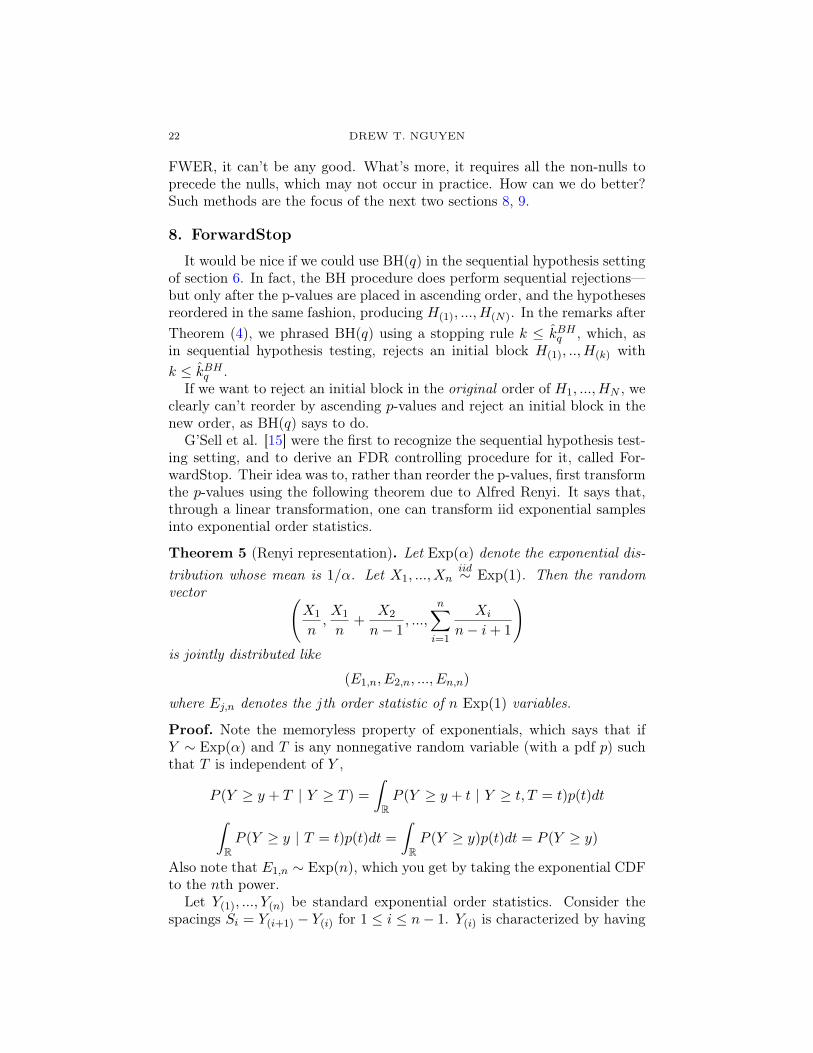
The authors performed numerical experiments to show that it was robustto correlation between the features, and they reported that the that thecovariance test statistic was not robust. We reproduce the plots from theirpaper in figure 1.

Figure 1. Experiments by T. Tony Cai and Ming Yuan foreT4

, computed from X generated by different ⇢.

10 DREW T. NGUYEN

Figure 1 shows QQ-plots of eT4

against the Gumbel. The authors choose� = (6, 6, 6, 0, 0, ...)T for n = 100, p = 50 and generated X from a multivari-ate normal distribution where Cov(Xi, Xj) = ⇢|i�j|. Then they generated eT

4

for 500 independent datasets. The points match up well with Gumbel; we seethat not only are they robust to ⇢ as big as 0.8, but that the approximationis quite good for moderately sized p.

Our treatment of the Lasso-G statistic in this section is theoretical; weprovide a proof of its null distribution (which was not provided by Cai andYuan). Our practical contribution is later, when we apply this statistic to theFDR control setting and show that it gets more power than the covariancetest (see section 10).

Recall Ak is the active set just before the kth knot, and let |Ak| be its car-dinality. Suppose variables enter the lasso model in the order {j

1

, j2

, ..., jp}and define Rjk(Ak) =

�

RSSAk� RSSA[{jk}

� �

�2, which is the drop in resid-ual sum of squares from OLS regression on only those variables in {Ak}versus {Ak} including the new variable entering the model. Then define theLasso-G test statistic:

eTk = Rjk(Ak)� 2 log(|Ak|c) + log log(|Ak|c) (12)

One can think of �2 log(|Ak|c) + log log(|Ak|c) a correction factor to justthe drop in RSS, which for the OLS problem is known to have a chi-squaredistribution. The factor corrects for the selection of {Ak}; without it wedon’t have an adaptive method.

Theorem 2 (Lasso-G test). Under H0k and with XTX = I,

eTkd! Gumbel(� log(⇡), 2) (13)

as p ! 1, with n > p, and their p-values are independent.

Proof. Let ˆ�A :=

ˆ�OLSA be the OLS solution regressed against just those

variables in A ✓ {1, ..., p}, and XA be X just including those columns. Then

RSSA = ||y �XAˆ�||2

2

and expanding the sum and applying XTX = I gives

RSSA = kyk22

� 2

ˆ�TAX

TAy + || ˆ�A||2

2

Again applying orthogonality, now using ˆ�OLSj = XT

j y, we simplify

RSSA = kyk22

� 2yTy + || ˆ�A||22

= || ˆ�A||22

� kyk22

so that the RSSA � RSSA[{j} for some j not in A is

RSSA � RSSA[{j} = || ˆ�A[{j}||22

� || ˆ�A||22

which is maximized over j by picking the one with |XTj y| the largest. As

for the lasso, in the case of orthogonal design, inspecting equations (10) tells


us that the jth variable to enter the model is also the one where |XTj y| is

largest, out of all those that have not yet been added. So thenRjk = max

m2Ack

Rm(Ak)

Classical regression theory says that each Rm(Ak), under the null, has a �2

1

distribution. So Rjk is a maximum of �2

1

, whose distribution we can getthrough extreme value theory.

Before we do that let’s note that the p-values are independent by the samereasoning as the proof of the covariance test. Also analogously to what wesaid in the covariance test, we only need to prove it for eT

1

, because wheneverwe assume H

0k to be true, we can always think of Rjk as a maximum orderstatistic of �2

1

, and we may as well do the proof for Rj1

.Let V

1

� V2

� ... � Vp be the order statistics of an absolute standardnormal. Then every Vk is equal in distribution to the U

(k) from the proof ofthe covariance test, and we can define W

1

= bp (V1

� ap) just as before andrecall we proved it is distributed as � log(E) for E a standard exponential,when ap = �

�1

(1 � 1/2p) and bp = 2p�(ap). The fact is that � log(E) ⇠Gumbel(0, 1).

Now by Example 1.1.7 in de Haan and Ferreira, we could have choseninstead different constants ap and bp and still gotten this result. Followingthe logic in that example (with a minor modification since we have absolutestandard normals, not standard normals)5 we can redefine

ap =p

2 log p� log log p+ log ⇡

2

p2 log p

bp =p

2 log p

and have the same result of asymptotic convergence hold. NowV1

+ apbp

=

V1

� apbp

+ 2

apbp

Clearly apbp

= 1+o(1). But also V1

� ap�

bp = W1

/b2p ! 0 almost surely, sincebp ! 1 and W

1

goes to a nondegenerate distribution. So V1

+ ap�

bp ! 2

almost surely, and then

V 2

1

� a2p = W1

·⇣

V1

+ ap�

bp

⌘

! 2 · Gumbel(0, 1) = Gumbel(0, 2)

But after explictly squaring a2p you can see a2p ⇡ 2 log(p) � log log(p) �log(⇡) for large p. Rearranging, and noting that under the null Rjk as �2

1

is distributed just like V 2

1

which is a squared normal, we have that eTk !Gumbel(� log(⇡), 2).

⇤5If we’d had standard normals we would write ap =

p2 log p� log log p+log 4⇡p

2 log p. According

to a paper of Hall [9], this is, in a supremum error sense the best choice of constants forthe standard normal (it converges fastest).

12 DREW T. NGUYEN

That’s as far as we’ll go for generation of p-values. Naturally this is not theend of that story; are there other statistics? Other tests? Other hypotheses?And are there methods that still have guarantees when XTX 6= I? Yes, ofcourse, to all; since the covariance test was proposed, there came to existsomething of a menagerie of methods, and they make up the field calledselective inference. We mention some of these methods at the end. However,the covariance test stands out as the field’s progenitor, and remains thesimplest test. Meanwhile, the lasso-G test was simply another, simpler wayto do the same thing, which may obtain better results under orthogonalityand remain robust outside of it.

4. Multiple Hypothesis Testing and the FDRWe turn to multiple hypothesis testing—the problem of how to combine

p-values to test multiple hypotheses, subject to false discovery concerns. Thepoint of this section is to illustrate those concerns.

Consider now a genome-wide association study, which has a disease inmind and searches the entire human genome for genes that might be riskfactors or causal factors for its development. There are tens of thousandsof genes to search through, and each kth gene corresponds to another nullhypothesis Hk—namely, does gene k contribute to the disease? As a differentexample, if one is searching for certain subsequences in a chromosome tounderstand the synthesis of a protein, the number of nulls towers into themillions [10].

Each hypotheses Hk has a p-value pk, and we reject, say, if pk < t, so t issome threshold. For N hypotheses, let V (t) N be a (unobserved) randomvariable equal to the number of false rejections.

Classically, to control type I error means to control for any mistake underthe null hypothesis, so for a multiple testing analogue we may wish to chooset so that P (V (t) � 1) < q for some desired q (this probability is called thefamily-wise error rate, or FWER). So we bound the probability that wefalsely reject even once. But when we have millions of null hypotheses this isan unreasonably stringent criterion, because as we consider more and morenulls, it becomes more and more likely that a null p-value is less than ↵ bychance. We could adjust t to make ↵ very small, but then we will hardlyever reject, even when we should. So we have lost power.

Large datasets in technology and in biology have led researchers to thefollowing attitude; making a few type I error type mistakes is not the end ofthe world. If we are interested the genes for which Hk is rejected, it is worthsome false positives to have the actual interesting genes be revealed.

Let R(t) be the total number of rejected hypotheses. There are somecompetitors for a looser criterion to control, but the standard one is thefalse discovery rate, or the FDR:

FDR(t) = E

V (t)

max(R(t), 1)

�

(14)


Type I error control becomes: Pick t so that FDR(t) q for some chosenthreshold q. This is a loose criterion; controlling an expectation means thatwe may do badly on FDR control on any one experiment, but that on averagewe do not.

5. Continuous-time Martingales and the Optional StoppingTheorem

We have defined the FDR, but we have not actually given procedures forhow to control it when testing N hypotheses.

Before we define these procedures and prove their FDR controlling prop-erties, we need some results on martingales. This is essentially because thequantity V (t)/t, and other similar quantities (where recall V (t) is our num-ber of false rejections at t and t is our threshold) turn out to be martingalesin t, or sub- or supermartingales. In any case, this allows us to apply theuseful optional stopping theorem.

We assume basic results from martingales in discrete time—specifically wewill assume the backwards martingale convergence theorem, which can bemostly proven by modifying the proof of the usual martingale convergencetheorem6.

Now we define martingales in continuous time, as well as some relatedconcepts. Note that conditional expectation is taken over �-algebras ratherthan events—one distinction is that a conditional expectation is a randomvariable.

Let (⌦,F , P ) be a probability space. We have the following definitions:

Definitions.

• A filtration is a collection {Ft}t�0

of �-algebras such that every Ft ✓F and Fs ✓ Ft for s < t.

• A stopping time is a random variable ⌧ : ⌦ ! [0,1] such that for allt, {! 2 ⌦ : ⌧(!) t} 2 Ft.

• A submartingale is a stochastic process {Xt}t2[0,1)

on (⌦,F , P ) with:� Xt 2 Ft. We say that {Xt} is adapted to {Ft}.� Xt 2 L

1

, i.e. E|Xt| < 1. We say that Xt is integrable.

� E[Xt|Fs] � Xs for s t. It follows that EXt � EXs.A supermartingale is the same thing, but with the third bullet pointreplaced with E[Xt|Fs] Xs for s t, and then EXt EXs.

• A martingale is a submartingale that is also a supermartingale.• A backwards (sub, super) martingale is the same as above, except the

filtrations satisfy Fs ◆ Ft for s < t. Equivalently, keep the filtrationsthe usual way, but index t starting at 0 and going to �1. (We will

6The usual martingale convergence theorem is probably the more “major” theorem, butbackwards martingales are important enough to be considered in detail in introductorytexts like [11]

14 DREW T. NGUYEN

only have use for the discrete case, where t can be identified with thenegative integers.)

• A stochastic process {Xt(!)}t�0

is right continuous if for all t, !,

lim

s#tXs(!) = Xt(!)

For some stochastic process {Xt}t�0

on (⌦,F , P ), we say the natural fil-

tration is defined by Ft = �⇣

S

t0t �(Xt0)

⌘

; the filtration generated by allrandom variables that occurred earlier than or at t.

The �-algebras of a natural filtration refer to information present at timet, because �(Xt) contains all measurable events whose occurrence we can de-termine by observing Xt, and conditioning on �(Xt) essentially produces arandom variable conditioned on all these events, weighted by their probabil-ities. It will be also be advantageous in proofs to append information asidefrom just the information contained in the process. Formally this means wegenerate Ft not just based on Xt, but based on an auxiliary random variableYt, too—or we can let Yt = y and condition on that event.

Our goal in this section is to prove the optional stopping theorem (forbounded stopping times) from continuous-time martingales for use in proofsin sections 6 and 8, which will allow us to simplify several calculations. Also,we use the discrete time analogue of this theorem in section 9, which is statedthe same way.

Our proof is modified from one given in [12], where a less general theoremis proved.

Let B � 0; define SB the set of all stopping times ⌧ such that ⌧ B withprobability 1.

Theorem 3 (Bounded Optional Stopping Theorem). Let {Xt}t�0

be a right-

continuous nonnegative submartingale. Then A = {X⌧ : ⌧ 2 SB, B � 0}isuniformly integrable

7, and

E[X�|F⌧ ] � X⌧ and E[X�] � E[X0

] (15)

for all ⌧,� 2 SB with �a.s.� ⌧ .

Equations (15) show that the submartingale properties that E[Xt|Fs] �Xs for s t and EXt � EXs generalize to random stopping times givenright continuity and a.s. boundedness of the stopping times. Without thesekinds of conditions, this need not hold; consider the discrete martingale withrespect to its natural filtration, where X

0

= 0 and Xi = Xi�1

+ ⇠i for i � 1

and ⇠i are all iid, and equal to 1 or �1 with equal probability. Then {Xi}is a simple random walk. However, if ⌫ is the first time X⌫ hits 1, thenEX⌫ = 1 6= EX

0

= 0, even though ⌫ can be shown to be a stopping time7In martingale theory, when this is satisfied they say that {Xt}t�0

is class DL. Wewon’t actually use class DL for anything, but it’s part of the statement of the theorem,and is important to be able to say a submartingale has a Doob-Meyer decomposition.


and almost surely finite. The problem here is that ⌫ is not almost surelybounded by some B.

Proof. Let ⌧ 2 SfB ✓ SB, where Sf

B is the set of stopping times such that ⌧takes only finitely many values, such as 0 t

1

< t2

< ... < tn B.First we show E[XB|F⌧ ] � X⌧ for ⌧ 2 Sf

B and B our nonrandom bound,in order to establish uniform integrability for Af

= {X⌧ : ⌧ 2 SfB}. This

holds because then X⌧ = |X⌧ | E[XB|F⌧ ]. The conditional expectationof the integrable random variable XB is integrable, so that the family Af

is dominated by an integrable function, which implies uniform integrability.After we show this, we move to general ⌧ 2 SB.

Let A 2 Ft. By the definition of conditional expectation, if E[X⌧ A] E[XB A] for any such A then we do have E[XB|F⌧ ] � X⌧ , so we show this.Since X⌧ =

Pnk=1

X⌧ {⌧ = tk}, we get the first equality, and then simplify:

E[X⌧ A] =

nX

k=1

E[X⌧ A {⌧ = tk}] =nX

k=1

E[Xtk A {⌧ = tk}]

Then, using that {Xt} is a submartingale, and applying once again thedefinition of conditional expectation (because {⌧ = tk} is an event in Ftk):

nX

k=1

Eh

E[XB A {⌧ = tk}|Ftk ]

i

=

nX

k=1

E[XB A {⌧ = tk}]

which is E[XB A], as needed.Now let ⌧ 2 SB. We define a sequence {⌧n} of stopping times by ⌧

1

= Band for n > 1, ⌧n = max {2�nd2n⌧e, ⌧n�1

, B}. These are strictly larger than⌧ and less than B and nonincreasing, and for each n only take finitely manyvalues, because the ceiling function only takes finitely many values until⌧n = B. So ⌧n 2 Sf , and we have ⌧n # ⌧ . By right continuity, this impliesthat X⌧n ! X⌧ (for any fixed !).

Fix ✏ > 0; writing out the definition of uniform integrability for Af , wehave K � 0 such that for every X⌧n

Eh

|X⌧n | · {|X| � K}i

✏

Applying DCT and taking n ! 1 we see that appending X⌧ to Af doesn’tbreak the uniform integrability. We can do this for all ⌧ and see that the setA = {X⌧ : ⌧ 2 SB} is uniformly integrable.

Now we show the martingale properties (15) hold. Let’s redefine ⌧n =

max {2�nd2n⌧e, ⌧n�1

,�}, setting ⌧1

= �. Since ⌧n is nonincreasing, {X⌧n}and its corresponding filtration define a discrete backwards submartingale.The statement of the backwards submartingale convergence theorem is thata discrete backwards submartingale has a limit both in a.s. (which we knowis X⌧ ) and in L1, and that this is less than or equal to limn E[V |F⌧n ], where

16 DREW T. NGUYEN

V is the first term of the backwards submartingale. X� is the first term, soX⌧n ! X⌧ lim

nE[X�|F⌧n ]

in both a.s. and L1.To use these formulas, we take conditional expectations:

X⌧ = E[X⌧ |F⌧ ] Eh

lim

nE[X�|F⌧n ]

�

�

�

F⌧

i

= lim

nEh

E[X�|F⌧n ]

�

�

�

F⌧

i

= lim

nE[X�|F⌧ ] = E[X�|F⌧ ]

where we can commute the limits because of L1 convergence and we use thelaw of total expectation at the end. This proves E[X�|F⌧ ] � X⌧ .

To show E[X0

] E[X�], just set ⌧ = 0 so that E[X�|F0

] � X0

, and takeexpectations of both sides:

Eh

E[X�|F0

]

i

= EX� � EX0

.

⇤Some final remarks. This is not the most general form of the optional

stopping theorem, either in discrete and continuous time; even if we revokeboundedness of the stopping times, there are other conditions we could im-pose so that equations (15) still hold. Lastly, we note that nonnegativitywas not required for equations (15) to hold.8

6. The Benjamini-Hochberg procedureWith the needed results from martingale theory in place, we are all ready

to set up to state and prove the Bejamini-Hochberg procedure for FDRcontrol [13], abbreviated the BH procedure, or BH(q).

Benjamini and Hochberg’s landmark 1995 paper, currently with around45000 citations on Google Scholar, first defined the FDR and the BH methodto control it. FDR has since become the mainstream criterion for multipletesting due to advances in data collection technology, and the BH procedurein particular has become a standard topic in applied statistics because of itssimplicity and practicality. In this section we define the procedure and proveit controls FDR, using essentially the martingale proof due to Storey et al.[14], which greatly simplified the original authors’. The martingale idea isto exploit the optional stopping theorem, and this idea crops up again andagain in the extensions and relatives of the BH procedure we give in sections8 and 9.

The setting for BH is N unordered null hypotheses H1

, H2

, ...HN , each ofwhich is associated with independent p-values p

1

, p2

, ..., pN . Some unknownnumber N

0

= ⇡0

N of these hypotheses are truly null hypotheses, and their8Actually, if {Xt} is a martingale, you don’t even need nonnegativity to show it’s of

class DL (see previous footnote.) At the step in the proof where we show X⌧ is dominated,we can instead show it’s equal to a conditional expectation over a sub �-algebra of F , aset which is always uniformly integrable.


corresponding p-values are therefore distributed as p0iiid⇠ Unif[0, 1], where

the 0 superscript denotes a null p-value and ⇡0

2 [0, 1] is called the nullproportion. The approach of BH is to specify an FDR controlling thresholdt such that we reject all p-values pi satisfying pi t.

Specifically let our total number of rejections be R(t) = #{pi t}. LetV (t) = #{pi t : pi is null} be the number of false rejections. The thresholdt is chosen to bound FDR(t) = E

h

V (t)/max(R(t), 1)i

, which is our analogueof type I error, by some q 2 [0, 1].

For p1

, ..., pN , define

[FDR(t) =

Nt

max(R(t), 1)

Then BH(q) prescribesˆtBHq := sup{0 t 1 :

[FDR(t) q} (16)

In particular we have[FDR(

ˆtBHq ) q. (17)

Theorem 4 (BH(q)). For the N hypotheses H1

, ..., HN , with independent p-

values p1

, ..., pN , we reorder the p-values to form the order statistics p(1)

, ..., p(N)

,

and order the N hypotheses the same way, labelling H(1)

, ..., H(k).

Fix q 2 [0, 1], and reject H(k) for p

(k) tBHq . This rule controls FDR at

level q.

Before we give the proof let’s make some remarks.First, the usual formulation of BH(q) is more simply stated; it just says

that for ordered p-values p(1)

... p(N)

, we define

ˆkBHq = max

⇢

k : p(k)

k

Nq

�

(18)

and we reject all H(k) with k ˆkBH

q . The random integer ˆkBHq is called a

stopping rule.The two formulations are equivalent because R(p

(k)) = k, so that [FDR(p

(k)) =

Np(k)/k, and then

p(

ˆkBHq )

= max

⇢

p(k) : p(k)

k

Nq

�

= max

n

p(k) :

[FDR(p

(k)) qo

Comparing the form of p(

ˆkBHq )

to ˆtBHq , we conclude p

(k) p(

ˆkBH)

(i.e. isrejected) if and only if p

(k) ˆtBHq , since p

(

ˆkBH)

ˆtBHq < p

(

ˆkBH+1)

.

Secondly, why have I chosen the name [FDR (where the hat suggests an

estimate)? Actually, it really is kind of a heuristic estimate of the true FDRas follows:

E

V (t)

max(R(t), 1)

�

⇡ EV (t)

Emax(R(t), 1)⇡ EV (t)

max(R(t), 1)

18 DREW T. NGUYEN

Since the denominator is an observed random variable, we can just estimateits expectation by its observed value. But what is the numerator? Thenull p values are uniform, so they lie within the rejection region [0, t] withprobability t; if there were just one null p-value pi, then EV (t) = P (pi t) =t. Since there are ⇡

0

N of them, EV (t) = ⇡0

Nt.Still ⇡

0

is unknown. We may “estimate” ⇡0

= 1

9 , and find that⇡0

Nt

max(R(t), 1)⇡ Nt

max(R(t), 1)=

[FDR(t)

So [FDR(t) is intuitively a kind of upward biased estimate of the true FDR,

so that we would expect the true FDR to be “probably” less than [FDR, and

bounding the latter should bound the former. This is precisely what BH(q)does.

The idea of bounding an estimate for the FDR is also present in section9; one can choose different kinds of estimates to derive different kinds ofmethods, and that is just what we do there.

Proof. We ultimately want to show that at the threshold t = tBHq , we have

FDR(tBHq ) q, and we say FDR is controlled at level q.

Let M(t) = V (t)/t, and consider the stochastic process {M(t)}0t=1

. Thebounds mean we think of M(1) as the starting point, with t ! 0. Definethe �-algebra Ft = �(V (s), R(s) : 1 � s � t). Then M(t) is adapted to thefiltration {Ft}0t=1

, because if we know V (t) we also know M(t). (Alternately,V (t) is Ft-measurable, so M(t) is as well.)

We show that M(t) is a martingale in backwards time10 (a calculationomitted in Storey et al [14].). M(t) is integrable because E|M(t)| = ⇡

0

N . Itremains to show that E[M(t)|Fs] = M(s)11 for 1 � s � t.

First, we compute E[M(t)|M(s)] := E⇥

M(t)|�(M(s))⇤

:

E[M(t)|M(s)] = E[M(t)|V (s), s] =1

tE[V (t)|V (s), s]

where we explicitly note our knowledge of s. Let p0i denote a null p-value.Conditional on V (s) and s, we have

V (t) = #{p0i : p0i t s} =

V (s)X

i=1

⇠i (19)

9There exist corrections [14] which properly estimate ⇡0

, rather than just setting it to1. Such methods yield greater power, but are not my focus.

10Not to be confused with backwards martingale; the first term of a martingale’s fil-tration is the smallest �-algebra of that filtration, and a backwards martingale’s is thelargest. F

1

is the smallest here.11This is why it makes sense to go backward in time. Conditioning on Fs, which is to

say, V (s), for 1 � s � t excludes all the null p-values above s, which restricts the numberof p-values we have left to classify by time t. On the other hand, knowing V (t) doesn’tgive us useful information about V (s).


where ⇠i is a random variable that’s 1 if p0i t and 0 otherwise.Unconditioned, p0i

iid⇠ Unif[0, 1]. Then conditioning on s, a routine calcu-lation gives that each p0i |{p0i s} iid⇠ Unif[0, s]. Additionally conditioningon V (s), which is to say the state of null p-values besides the ith, gives noadditional information because the pi are independent.

Now just compute:12

1

tE[V (t)|V (s), s] =

1

t

V (s)X

i=1

E⇠i =1

t

V (s)X

i=1

P (p0i t) =1

tV (s)P (p0i t) (20)

=

1

tV (s)

t

s=

V (s)

s= M(s)

where t/s is the CDF of Unif[0, s].So we have E[M(t)|M(s)] = M(s). In addition, E[M(t)|M(s0), s s0] =

M(s), because the knowledge of every V (s0) means we know which p0i > tas long as s < p0i s0 (because we know the s0 such that V (s0) has jumps),and therefore we know V (t) does not count them. However, whether or notV (s) counts the p0i s, of which there are V (s), is still random; this is thecontent of equation (19). Lastly, knowing R(s) when we know V (s) meanswe know which were the non-null p-values as well, but that’s irrelevant toM(t). So we have shown E[M(t)|Fs] = M(s).

tBHq is clearly bounded, and it is a stopping time because if we know R(s)

for all s � t, then we know [FDR(s) (in particular we know whether or not

it’s less than q). This is enough to know if tBHq t.

However, M(t) is not right continuous (taking “going right” to mean from1 to 0). No matter; because the p0i come from a continuous distribution,we can redefine V (t) = #{p0i : p0i < t} using strict inequality13 and defineM(t) using this, and they will be equal almost surely, so that we have a rightcontinuous version of M(t).

Applying optional stopping for martingales,

EM(tBHq ) = EM(1)

1

tBHq

EV (tBHq ) = EV (1) = N

0

where recall N0

is the true number of nulls. From the definition of [FDR, we

also have

max(R(tBHq ), 1) =

NtBHq

[FDR(tBH

q )

� NtBHq

q

12Saying that we condition on a random variable is shorthard for saying we conditionon the �-algebra it generates. However, one can show that it corresponds correctly withour intuition, so we can use it to do calculations without fear, as I’m doing here.

13If the original problem involved discrete distributions, the p-values may not havecontinuous distributions. Indeed, we are implicitly assuming they are all continuous.

20 DREW T. NGUYEN

where the inequality is implied by (17).Putting these two together, and noting N

0

N we finally have

FDR(tBHq ) = E

"

V (tBHq )

max(R(tBHq ), 1)

#

q

NE"

V (tBHq )

tBHq

#

= qN

0

N q (21)

⇤

7. Sequential Hypothesis TestingSo much for unordered hypothesis testing. We have now defined FDR

and proved a procedure that controls it, called the BH procedure. However,we will actually have no use for BH directly. We include it because it isarchetypal; its proof is the simplest example of an optional stopping basedproof we have, not to mention it would be remiss to omit such a landmarkresult.

However, our real interest is in sequential hypothesis testing: we imposethe condition that we can only reject hypotheses in a certain order, andthe reordering of the p-values as done in BH are impossible in this case.Regardless, one can think of the forthcoming procedures as variations on theBH theme.

To motivate the problem, note that in section 3, the null hypothesis wasH

0

: supp(�⇤) ✓ Ak, where Ak was the active set just before the kth knot.

If there are N knots (in fact, recall N = p for orthogonal X), then we mayindex the null hypotheses:

H1

: supp(�⇤) ✓ A

1

H2

: supp(�⇤) ✓ A

2

...HN : supp(�⇤

) ✓ AN

(22)

and in the setting of the lasso with orthogonal X, we have A1

✓ A2

... ✓ AN

because variables only enter and never leave.Rejecting a hypothesis means that we believe the model Ak selected at

that stage is wrong, so we increase �, reach another knot, and therefore addanother variable and consider Ak+1

. Since the falsehood of Ak implies thefalsehood of Ak0 for all k0 < k, the rejection of Ak implies rejection of allAk0 . So when we reject hypotheses, we can only reject sequentially; that is,we cannot reject A

1

and A3

without rejecting A2

as well. Subject to thiscondition, we would like to derive FDR controlling procedures.

Let’s formalize the main idea. We have H1

, ..., HN hypotheses in a spe-cific order and associated p-values, where rejection of hypotheses is not si-multaneous but rather goes from the first to the last. Any rejection rule isconstrained by the following requirement: if we reject, we may only reject aset of hypotheses of the form {H

1

, ..., Hk} for some k N .


This restriction of rejecting hypotheses in order is called sequential hy-pothesis testing, because of the enforced sequence {Hk}Nk=1

. Each hypothesisis associated with a p-value, whose generation was the topic of section 3. Wenow consider them as generated from some distribution, and focus on theproblem of combining them for testing in this more restricted setting, whichis the natural one for the null hypotheses of equations (22).

Each FDR-controlling method we consider will define a stopping rule ˆk,which is a function of the p values, and tell us to reject all H

1

, ..., Hˆk. We

had one for BH(q) as well, but now let’s make it a formal definition.

Definition. A stopping rule for a sequential hypothesis testing problemH

1

, ..., HN with associated p-values p1

, ..., pN is any function ˆk of the N p-values which takes values in {0, 1, ..., N}, and rejects all hypotheses Hk withk ˆk.

So in sequential testing, we only reject an initial block of hypothesesH

1

, ...Hˆk, up to the index returned by the stopping rule.

To illustrate the concept, we define probably the simplest stopping rulethat works. It simply rejects until the first time a p-value exceeds q.

Proposition. Suppose either that for some unknown 1 k0

N , every

Hk0

, ..., HN is null, or that none of our hypotheses are null. Then define the

stopping rule

ˆk = min{k : pk > q}� 1

for some q 2 [0, 1]. This controls FDR at level q. In fact, it controls

P (V � 1) at level q.

Proof. Recall V is false rejections and R is all rejections. The quantityP (V (q) � 1) was mentioned in section 3 as an alternative to the FDR as atype-I-esque criterion. In fact P (V (q) � 1) � FDR, because R(q) � V (q),so

{V (q) � 1} � V (q)

max(R(q), 1)

and taking expectations on both sides shows that P (V (q) � 1) � FDR(q).The given stopping rule controls P (V (q) � 1) because

P (V (q) � 1) P (pk0

q) = q

where k0

is the first null hypothesis, and null p-values are uniform.⇤

The quantity P (V � 1) is known as the FWER, the family-wise errorrate. Before Benjamini and Hochberg proposed the FDR as an alternativecriterion, researchers used the FWER, and had a hard time because (as dis-cussed in section 4) such a criterion is too stringent and sucks away power asthe number of hypotheses increases. Since this simple stopping rule controls

22 DREW T. NGUYEN

FWER, it can’t be any good. What’s more, it requires all the non-nulls toprecede the nulls, which may not occur in practice. How can we do better?Such methods are the focus of the next two sections 8, 9.

8. ForwardStopIt would be nice if we could use BH(q) in the sequential hypothesis setting

of section 6. In fact, the BH procedure does perform sequential rejections—but only after the p-values are placed in ascending order, and the hypothesesreordered in the same fashion, producing H

(1)

, ..., H(N)

. In the remarks afterTheorem (4), we phrased BH(q) using a stopping rule k ˆkBH

q , which, asin sequential hypothesis testing, rejects an initial block H

(1)

, .., H(k) with

k ˆkBHq .

If we want to reject an initial block in the original order of H1

, ..., HN , weclearly can’t reorder by ascending p-values and reject an initial block in thenew order, as BH(q) says to do.

G’Sell et al. [15] were the first to recognize the sequential hypothesis test-ing setting, and to derive an FDR controlling procedure for it, called For-wardStop. Their idea was to, rather than reorder the p-values, first transformthe p-values using the following theorem due to Alfred Renyi. It says that,through a linear transformation, one can transform iid exponential samplesinto exponential order statistics.

Theorem 5 (Renyi representation). Let Exp(↵) denote the exponential dis-

tribution whose mean is 1/↵. Let X1

, ..., Xniid⇠ Exp(1). Then the random

vector

X1

n,X

1

n+

X2

n� 1

, ...,

nX

i=1

Xi

n� i+ 1

!

is jointly distributed like

(E1,n, E2,n, ..., En,n)

where Ej,n denotes the jth order statistic of n Exp(1) variables.

Proof. Note the memoryless property of exponentials, which says that ifY ⇠ Exp(↵) and T is any nonnegative random variable (with a pdf p) suchthat T is independent of Y ,

P (Y � y + T | Y � T ) =

Z

RP (Y � y + t | Y � t, T = t)p(t)dt

Z

RP (Y � y | T = t)p(t)dt =

Z

RP (Y � y)p(t)dt = P (Y � y)

Also note that E1,n ⇠ Exp(n), which you get by taking the exponential CDF

to the nth power.Let Y

(1)

, ..., Y(n) be standard exponential order statistics. Consider the

spacings Si = Y(i+1)

� Y(i) for 1 i n� 1. Y

(i) is characterized by having


above it n � i order statistics Y(i+1)

, ..., Y(n), so Y

(i+1)

can be thought of asdistributed as E

1,n�i independently from Y(i), conditioned on E

1,n�i � Y(i).

Then

P (Si > s) = P (E1,n�i � Y

(i) > s | E1,n�i � Y

(i))

= P (E1,n�i > s+ Y

(i) | E1,n�i � Y(i))

= P (E1,n�i > s)

where we have used that E1,n�i is exponential. So Si ⇠ Exp (n� i).

Now (n�i)Si = (n�i)(Y(i+1)

�Y(i)) := X 0

i ⇠ Exp(1). Then Y(i+1)

�Y(i) =

X 0i/(n� i). Using the algebraic identity

j�1

X

i=0

Y(i+1)

� Y(i) = Y

(j) ⇠ Ej,n

where we may define Y(0)

= 0 and X 00

= nY(1)

, substituting in X 0i/(n � i)

yields the result.⇤

If we can convert exponential random variables to exponential order sta-tistics, we can convert uniform p-values pk to uniform order statistics p0kby converting to exponential (through inverse transform sampling), apply-ing Renyi representation, and then converting back (through the probabilityintegral transform). The uniform order statistics act like ordered p-values,which allows us to apply BH(q). This idea translates more or less immedi-ately to a proof if all the non-null hypotheses are assumed to precede thenulls, which may not be the case in practice. Regardless, the main idea isstill present in the proof of FDR control for the ForwardStop procedure pro-posed by G’Sell et al., named so because it scans the p-values in a forwarddirection.

Theorem 6 (ForwardStop). Suppose we have N ordered hypotheses with

associated independent p-values, H1

, ..., HN and p1

, ..., pN and a subset H0

✓{1, ..., N} which indexes the null hypotheses (so that pi

iid⇠ Unif[0, 1] for all

i 2 H0

). Let 0 < q < 1.

Define the stopping rule

ˆkFq = max

(

k 2 {1, ..., N} :

1

k

kX

i=1

� log(1� pi) q

)

(23)

Then this controls FDR at level q.

Proof. Define Yi = � log(1 � pi), which is standard exponential randomvariables if pi is null. Then define

Zk =

lX

i=1

Yi⌫(i)

24 DREW T. NGUYEN

where ⌫(i) = #{j 2 {i, ..., N} : j 2 H0

}, the number of nulls from i to N .If all the hypotheses had been truly null, then ⌫(i) = N � i + 1, and Zk

would be an exponential order statistic by Renyi representation. That is notthe necessarily the case under our assumptions, but we can still break thesum into two terms and apply Renyi representation to one of them.

Let N0

= #{H0

}, the number of null hypotheses. Starting from k = 1

and going to k = N , take the p-value pk and give it a label: A(i) if it’s theith non-null from {p

1

, ..., pk} you’ve seen, and N (i) if it’s the ith null. Thereare N

0

nulls and N �N0

non-nulls; we can re-express Zk as

Zk =

k�(N0

�⌫(k+1))

X

i=1

YA(i)

⌫(A(i))

+

N0

�⌫(k+1)

X

i=1

YN (i)

N0

� i+ 1

where N0

�⌫(k+1) is the number of nulls from 1 to k (defining ⌫(N+1) = 0)and where we’ve simplified ⌫(N (i)

) = N0

� i+ 1 when pi is null.Define Y 0

i = YN (i) , which is standard exponential and independent fromthe other Y ’s. By Renyi representation, the second summation is distributedas some EN

0

�⌫(k+1),N0

variable.Again consider the ideal situation with all the hypotheses truly null and Zk

a exponential order statistic. Then defining p0k = 1�e�Zk would turn p0k intoa uniform order statistic (and 1� p0k = e�Zk are the uniform order statisticsin the opposite order). We’re not in the ideal situation, but regardless, wedefine p0k as such anyway. Then we have 1� p0k equal to e�Zk , and

1� p0kd= exp

8

<

:

�k�(N

0

�⌫(k+1))

X

i=1

YA(i)

⌫(A(i))

9

=

;

· U⌫(k+1),N0

where U⌫(k+1),N0

is the ⌫(k+1)th standard uniform order statistic out of N0

.Defining r(k) = exp

n

�Pk�(N0

�⌫(k+1))

i=1

YA(i)

⌫(A(i))

o

and noting that subtractinguniform order statistics from 1 gives uniform order statistics in the oppositeorder, we re-express

1� p0kd= r(k)(1� UN

0

�⌫(k+1),N0

)

So the p0k may not be uniform order statistics, but at least for the null p’s,we can read off that they are closer to 1 than uniform order statistics. Why?Letting p00k := p0N (k) , we have

1� p00kd= r(N (k)

)(1� Uk,N0

)

because N0

� ⌫(k + 1) is the number of nulls from 1 to k, and the numberof nulls N

0

� ⌫(N (k)+ 1) from 1 to N (k) is k. Now since 0 r(k) 1, we

imagine shrinking the difference between 1 and Uk,N0

. In other words, thep00k are stochastically larger than uniform.


With this knowledge we attempt to apply BH(q) to the p0k, as in equation(16), defining R(t) = #{p0i t} and V (t) = #{p0i t : i 2 SN}. Then FDRand [

FDR are also defined analogously as in section 6.Now set

tFq := sup{0 t 1 :

[FDR(t) q}

using these definitions for R and V . We wish to reject all Hk with p0k tFq .Analogously to the proof of BH(q), for the same filtration, we use a mar-

tingale idea, but this time we actually show that M(t) = V (t)/t is a sub-martingale.

Conditional on V (s), for s � t, express V (t) as in equation (19):

V (t) = #{p00i : p0i t s} =

V (s)X

i=1

⇠i

with ⇠i a random variable that’s 1 if p00i t and 0 otherwise. We know thep00i are stochastically larger than uniform order statistics, but V (t) has thesame value even if we permute the order of the p00i randomly, and if we do so,the shuffled p00i will each be stochastically larger than the standard uniform.This is because one can imagine they were they initially sampled iid froma uniform, made into order statistics, and then increased by some functionof r(N (k)

) that depends only on the nonnulls. Then shuffling them againwill break any effect ordering has on their distribution, but the effect of rremains.

Suppose we have done this. Now compute E[M(t)|M(s)] as in (20):

1

tE[V (t)|V (s), s] =

1

t

V (s)X

i=1

E⇠i =1

t

V (s)X

i=1

P (p00i t) =1

tV (s)P (p00i t)

and then using that each p00i is stochastically larger than uniform, whichmeans that their CDF is smaller,

1

tV (s)P (p00i t) 1

tV (s)

t

s=

V (s)

s= M(s)

so that E[M(t)|M(s)] M(s). Then, following exactly similar reasoning tothe proof of BH(q) in section 6, conditioning on Fs we see that M(t) is asubmartingale. Because tFq is bounded and can be verified, as in section 6, tobe a stopping time, (and because, assuming continuity of the transformed p-values p0, we can redefine V (t) with strict inequality to get right continuity,as in section 6), we can essentially rewrite equation (21) all over, so thatrejecting all Hk such that p0k tFq will control FDR.

However the theorem presented ForwardStop using an integer stoppingrule, not a stopping time. Because we are applying BH(q) to the p0 values,we can use equation (18) to see that rejecting based on p0k tFq is equivalent

26 DREW T. NGUYEN

to rejecting based on all k ˆkq, where

ˆkq = max

⇢

k : p0k k

Nq

�

= max

(

k : 1� exp

"

�kX

i=1

Yi⌫(i)

#

k

Nq

)

(24)

However, not only is ˆkq not equivalent to the rule proposed by the theorem, itis not even computable because it depends on knowledge of ⌫(k). To rectifythis, we can append to the original untransformed list p

1

, ..., pN additionalnull p-values (i.e. standard uniform) pN+1

, ..., pN 0 . The procedure outlinedso far still applies for any N 0 � N ; that is, letting tFq,N 0 be the resultingstopping time, FDR(tFq,N 0) q. Therefore, by DCT,

lim

N 0!1FDR(tFq,N 0) = lim

N 0!1E

V (tFq,N 0)

max(R(tFq,N 0), 1)

= E"

lim

N 0!1V (tFq,N 0)

max(R(tFq,N 0), 1)

#

q

so the rule obtained by taking N 0 ! 1 controls FDR if indeed we obtainsome rule. We can compute this rule through ˆkq. Letting ⌫N 0

(i) denote ⌫ inthis setting, we note it behaves like N 0 for large N 0. Likewise N +N 0 ⇡ N 0for large N 0. So taking limits in (24),

lim

N 0!1ˆkq = lim

N 0!1(N +N 0

)max

⇢

k : p0k k

Nq

�

= max

(

k : N

1� exp

"

�kX

i=1

YiN

#!

kq

)

= max

(

k :

kX

i=1

Yi kq

)

=

ˆkFq

a rule to which corresponds the random variable

lim

N 0!1V (tFq,N 0)/max(R(tFq,N 0), 1)

so that we were justified in applying DCT, and which matches the rulespecified in the theorem.

⇤

In this section we presented a method called ForwardStop which usesp-values to control FDR in a sequential hypothesis testing setting. At thispoint, the reader could take the statistics from section 3 on a model selectionproblem, turn them into p-values, and apply them with ForwardStop. ButForwardStop is not the only way to control FDR for sequential hypotheses,as we see in the next section.


9. Accumulation test procedures, SeqStep, and HingeExp

Consider the ForwardStop stopping rule ˆkFq . Specifically, forget about theRenyi and order statistic justification and consider the form ultimately ar-rived at in equation (23). Why should we believe, intuitively, that a functionlike � log(1� pi) would work—as opposed to its cube, say? In this section,we show that ForwardStop is part of a class of FDR controlling methodscalled accumulation tests (though what we actually prove is that accumula-tion tests control something similar, to but slightly larger than, the FDR,and ForwardStop is special because it controls FDR exactly).

Let FDP = V/max(R, 1), so that FDR = E(FDP). The idea of For-wardStop is to reject as much as possible—hence the max—while control-ling a certain quantity, namely 1

k

P

log

⇣

1

1�pi

⌘

. It’s reasonable to controlthis quantity because its expectation actually acts an upper bound of FDP(thereby kind of an overestimate of the FDR), so if it’s bounded above, thenso might FDP/FDR.

It’s an upper bound of FDP because null p-values pi have the pdf f(x) = 1

on [0, 1], so under the null

E log

✓

1

1� pi

◆

=

Z

1

0

log

✓

1

1� pi

◆

= 1

and we have

1

k· E"

kX

i=1

log

✓

1

1� pi

◆

#

� 1

k· E2

4

X

null ik

log

✓

1

1� pi

◆

3

5

=

V (k)

k

where k represents the value taken by our stopping rule, and stopping rulessay to reject all Hi with i k. So R(k) = k.

This intuition isn’t unique to ForwardStop; indeed, any function h :

[0, 1] ! [0,1) such that p ⇠ Unif[0, 1], and

E[h(p)] =Z

1

0

h(p)dp = 1

will have a corresponding rule

ˆkhq = max

(

k :

1

k

kX

i=1

h(pi) q

)

where (1/k)Pk

i=1

h(pi) is an overestimate of the FDP, and ˆkhq = 0 if it’sotherwise undefined.

Any h satisfying these properties is called an accumulation function; For-wardStop just sets h(p) = log(

1

1�x). We formalize the definition, howeversimple:

Definition. Let h : [0, 1] ! [0,1) be such thatR

1

0

h(p)dp = 1. Then wecall h an accumulation function.

28 DREW T. NGUYEN

This generalization was first noticed by Li and Barber (2015) [16], whostated and proved all the theorems in this section. Now before we state themain theorem of this section, we first define the modified FDR.

Definition. For c � 0, Eh

V (k)�

(c + R(k))i

is the modified FDR with pa-rameter c, denoted mFDRc. It is equal to the FDR when c = 0 and strictlysmaller than the FDR otherwise.

Of course, if k is a stopping rule, we can just write R(k) = k.Note that if R(k) the number of rejections is moderately large with c quite

small, this is not too far from the FDR, but otherwise, controlling mFDR isweaker than controlling FDR and has the potential to be much weaker. Nowhere’s the main theorem. The setting is as in theorem 6. Suppose we haveN ordered hypotheses with associated independent p-values, H

1

, ..., HN andp1

, ..., pN and a subset H0

✓ {1, ..., N} which indexes the null hypotheses(so that pi

iid⇠ Unif[0, 1] for all i 2 H0

).

Theorem 7 (Accumulation tests). Let h be an accumulation function and

let q 2 (0, 1) be a target FDR control level. Fix C > 0, and define the

stopping rule

ˆkhq = max

(

k 2 {1, ..., N} :

1

k

kX

i=1

h(pi) q

)

Then

mFDRC/q(ˆkhq )

qR

1

t=0

min(h(t), C)dt

This isn’t as straightforward as ForwardStop. Notice that h does notdepend on C; in fact, nothing depends on C except for the final control ofthe mFDR. In [16] C is simply taken to be 2. Also, the denominator of theright hand side is strictly less than 1, so we’ve lost exactly control at level q,and the quantity on the left side depends on q, as

mFDRC/q = E

V�

✓

C

q+R

◆�

Taking q really, really small will tend to shrink the mFDR compared tothe FDR on the left hand side. As for the right-hand side, we can get controlat q if we pick h(t) to be bounded and C to be its supremum, because thenthe denominator is 1. However, if the supremum is large, then the mFDR ismuch smaller than the actual FDR again14. So we see we must be reasonablewhen controlling mFDR, either picking h that is bounded by a small numberor applying accumulation tests in situations where we will reject a moderateamount.

14Aside from this situation of bounded functions, where you can say something aboutexact control, there’s no reason to “pick” different C; mFDR control holds true for all ofthem and the inequalities for different C seem equally useful.


I will defer the proof of this theorem to later, in favor of discussion now. Ittakes several lemmas and the proofs are not so terribly interesting, thoughI include them for completeness. The results, not the proofs, are the in-teresting thing here (one distinction between mathematics and statistics, Isuppose).

Here are a few things to say about the accumulation test procedures.• Is exact control of FDR important? In [16] Li and Barber also pro-

posed a modified version of this method that gives exact control ofthe FDR, but I do not consider it here, because it saps away power.In section 10 we find that control of the modified FDR seems to notbe so bad, and at least for that experiment we never exceeded thenominal level.

• The choice of h. We already see it might be advantageous to chooseh to be bounded, for FDR control reasons. But what about power?As we march along k, we add up the values h(pi) until we spill overq, and we don’t want a correct rejection to help accumulate evidencethat we should stop rejecting. So h(pi) or Eh(pi) should be small onthe non-nulls. Knowing the non-null distributions is impossible inprinciple, but today there are empiricial bayes methods that can doit [17], though they are not my focus.

• Where does ForwardStop fit in? We’ll define two useful methods inthis section, called SeqStep and HingeExp, both of which have morepower than ForwardStop as seen in section 10. But they only controla modified FDR. To me so far it has seemed to be a worthwhilecompromise because the power gains are large, but in a small signalsetting, or when there are many nulls and few rejections we may wantto use ForwardStop, or if we want to take q very small and rejectstringently, because it has good power and controls FDR exactly.

We continue deferring the proof of theorem 7 to define the SeqStep [18]and HingeExp [16] stopping rules.Definition (SeqStep). In Theorem 7, take

h(pi) = C ·n

pi > 1� 1

C

o

So the definition of SeqStep depends on your choice of C; it is named forbeing a step function for sequential testing. The good thing about SeqStepis that in the class of bounded functions, it is in some sense the “best” choice,given a reasonable condition on the non-nulls.Proposition. Let hS be the accumulation function corresponding to SeqStep

where C > 0 is chosen. Consider any other accumulation function h bounded

above by C. Suppose the non-null p-values pi have a density fi : [0, 1] ![0,1), where fi is nonincreasing.

Then on those non-null p-values,

Eh(pi) � EhS(pi)

30 DREW T. NGUYEN

In the most recent bullet points we said that we should keep Eh(pi) small,and by this proposition SeqStep does just that.15 We also note that thecondition that fi is nonincreasing is reasonable, because if a p-value is trulynot null, it should have probability weight towards the low end of [0, 1], notthe high end.

Proof of Proposition.

Eh(pi)� EhS(pi) =Z

1

0

�

h(t)� hS(t)� · fi(t) dt

=

Z

1�1/C

0

�

h(t)� 0

� · fi(t) dt+Z

1

1�1/C

�

h(t)� C� · fi(t) dt

=

Z

1�1/C

0

h(t) · fi(t) dt�Z

1

1�1/C

�

C � h(t)� · fi(t) dt

�Z

1�1/C

0

h(t)fi(1�1/C) dt�Z

1

1�1/C

�

C�h(t)�

fi(1�1/C) dt (fi is non-increasing)

= fi(1� 1/C) ·"

Z

1

0

h(t) dt�Z

1

1�1/CC dt

#

= fi(1� 1/C) · [1� 1] = 0.

⇤One remark. It is true that in the case of Eh(pi) � EhS(pi) = 0, then

h = hS almost everywhere, but we leave the explanation to [16].Now let’s define HingeExp. Its name comes from the fact that it looks

sort of like hinge loss from machine learning.

Definition (HingeExp). In Theorem 7, take

h(pi) = C log

✓

1

C · (1� pi)

◆

n

pi > 1� 1

C

o

So HingeExp also depends on your choice of C. This function, whichlooks sort of like a fusion of ForwardStop and SeqStep, was proposed in[16] to combine the BH(q) heritage of ForwardStop with the optimality ofSeqStep. There’s currently not much to prove about it in particular, but itworks really quite well.

Now we return to the proof of the main Theorem 7.Unlike the proofs given in other sections, the proofs in this section 9 will

follow extremely closely the original presentation in [18] and [16], whichwere very clear and left out very little (and which shared an author). Infact, I will be the one to leave things out; I will ask the interested reader to

15Of course this is not a proof that SeqStep actually has better power. In fact thereis a proof in [18] which says that, given some somewhat technical conditions, that ifEh

1

(pi) > Eh2

(pi) on the non-nulls then asymptotically greater power is achieved. Theproof is also somewhat technical (and very long) so we have left it out. Empirically weshall see the power gains.


refer to those references for the some of the omitted calculuations, which arepresented with satisfying detail there.

We begin by proving a few lemmas.

Lemma 2. Fix c 2 (0, 1). Let N (0)

be the largest element of H0

. For

0 k ˆN , put V +

(k) = #{j 2 H0

: 1 j k, pj c} and V �(k) =

#{j 2 H0

: 1 j k, pj > c}. Let Fk be the filtration generated by all the

non-null p-values as well as V ±(k0) for all k0 � k. Then the process

M(k) =V +

(k)

1 + V �(k)

is a supermartingale running in backwards k, adapted to Fk, and for any kwe have

E [M(k)] c

1� c

Proof. We assume H0

= {1, ..., bN} for some bN . The proof for the generalcase is identical, but messier.

Because we know all the nonnulls whenever we condition on Fk, we knowwhether or not k is null. If it is null then

M(k � 1) =

V +

(k)� I

1 + V �(k)� (1� I)

=

V +

(k)� I

min(V �(k) + I, 1)

where I = pkc. Otherwise if it is not null M(k) = M(k�1). Conditioningon Fk tells us nothing more about I. What it does tell us however is fork0 � which of the null pk0 was below c because then V (k0) goes up a notchwhen it does. Excluding those from consideration, at k we have

P (I = 1) =

V +

(k)

V +

(k) + V �(k)

where the denominator is just the total number of nulls left to consider bystep k and the numerator is how many of them are known to be less than c,that is to say, how many we’re allowed to pick from.

We’d like to calculate E [M(k � 1)|Fk]. This is easily done by weight-ing the null possibilities by P (I = 1) and P (I = 0); we then find thatE [M(k � 1)|Fk] M(k), which establishes the supermarginale property. Iomit the actual calculation and leave it for the reference [18].

To show the bound EM(k) = Eh

V +

(k)1+V �

(k)

i

c1�c , we let V (k) = V +

(k) +

V �(k) be the number of nulls from 1 to k (which is to say, the number of

false rejections), and re-express

E

V +

(k)

1 + V �(k)

�

= E

V +

(k)

V (k)� V +

(k) + 1

�

where V +

(k) ⇠ Binomial(V (k), c). Since the probability mass function isknown, computing this expectation is a routine exercise; nevertheless it canbe found in [18], though I omit it here.

32 DREW T. NGUYEN

The calculation proves the bound. ⇤

Corrolary. Let B1

, ..., BN 2 {0, 1} be independent, with Biiid⇠ Ber(⇢) for

i 2 H0

. Let {Fk}1k=N be a filtration in reverse k such that

• Bi 2 Fk for all i /2 H0

, and for all i > k with i 2 H0

• Pik,i2H0

Bi 2 Fk

• The null Bi are exchangeable conditioned on Fk

Then

M(k) =1 + V (k)

1 +

P

ik,i2H0

Bi

is a supermartingale adapted to Fk and EM(k) 1/⇢ for all k.

Proof. Set ⇢ = 1�c, where c is as in Lemma 2. Then identifyP

ik,i2H0

Bi

with V �(k) from Lemma 2. Let M 0

(k) be the supermartingale from Lemma2. Since a supermartingale plus a constant is still a supermartingale,

1 +M 0(k) = 1 +

V +

(k)

1 + V �(k)

=

1 + V +

(k) + V �(k)

1 + V �(k)

=

1 + V (k)

1 + V �(k)

= M(t)

is still a supermartingale. Also,

EM(k) = 1 + EM 0(k) 1 +

c

1� c=

1

1� c=

1

⇢.

⇤Lemma 3. Pick C > 0. Let a

1

, ..., aN � 0 and let h be an accumulation

function. Define

ˆk = max

(

k 2 {1, ..., n} :

kX

i=1

h(pi) ak

)

setting

ˆk = 0 if it’s otherwise undefined. Then

E"

1 + V (

ˆk)

C +

P

iˆk,i2H0

h(pi)

#

1

R

1

0

min(h(t), C)dt

Proof. Define additional variables Uiiid⇠ Unif[0, 1] independently from the

pi’s, andBi = {Ui h(pi)

�

C}Then conditional on the p

1

, ..., pN , the Bi are independently

(Bi|p1, ..., pN )

indep⇠ Ber✓

min

✓

h(pi)

C, 1

◆◆

= Ber✓

min(h(pi), C)

C

◆

(25)

Also, not conditioned on anything the null Bi are Bernoulli(⇢), where

⇢ = E

max(h(pi), C)

C

�

=

1

C

Z

1

0

max(h(pi), C)dt


We’d like to use the corollary. The filtration that works is where Fk isgenerated by knowing (pi, Ui) for i > k for i 2 H

0

and all the (pi, Ui)

when i /2 H0

. One can verify that ˆk is a stopping time with respect to thisfiltration. Then the corrolary, plus optional stopping16, says

EM(

ˆk) = E"

1 + V (

ˆk)

1 +

P

iˆk,i2H0

Bi

#

1

⇢=

1

1

C

R

1

0

min(h(pi), C)dt(26)

Next, we show

C · E"

1 + V (

ˆk)

C +

P

iˆk,i2H0

h(pi)

#

E"

1 + V (

ˆk)

1 +

P

iˆk,i2H0

Bi

#

which will prove the lemma when combined with (26).

E"

1 + V (

ˆk)

1 +

P

iˆk,i2H0

Bi

#

= E"

E"

1 + V (

ˆk)

1 +

P

iˆk,i2H0

Bi

�

�

�

p1

, ..., pN

##

= E"

(1 + V (

ˆk)) · E"

1

1 +

P

iˆk,i2H0

Bi

�

�

�

p1

, ..., pN

##

� E

2

4

(1 + V (

ˆk)) · 1

Eh

1 +

P

iˆk,i2H0

Bi

�

�p1

, ..., pN

i

3

5

where we’ve applied Jensen’s inequality to 1/x.Then by (25)

= E

2

4

1 + V (

ˆk)

1 +

P

iˆk,i2H0

max(h(pi),C)

C

3

5 � C · E"

1 + V (

ˆk)

C +

P

iˆk,i2H0

h(pi)

#

⇤Finally we can prove the theorem.

Proof of Theorem 7.

E[mFDPC/q(ˆkh)] = E

"

V (

ˆkhq )

C/q + ˆkhq

#

= E

2

4

V (

ˆkhq )

C +

P

ˆkhqi=1

h(pi)· C +

P

ˆkhqi=1

h(pi)

C/q + ˆkhq

3

5

By definition of ˆkhq , and then simplifying,

E

2

4

V (

ˆkhq )

C +

P

ˆkhqi=1

h(pi)· C + qˆkhq

C/q + ˆkhq

3

5

= q · E2

4

V (

ˆkhq )

C +

P

ˆkhqi=1

h(pi)

3

5

16We proved it for submartingales. It’s also true for supermartingales because you canjust multiply by negative signs to turn a supermartingale to a submartingale, apply thetheorem, and then multiply by another minus.

34 DREW T. NGUYEN

(now we can think of the term as an estimate of mFDP.) Add 1 to the topand remove terms from the bottom to get

q · E"

1 + V (

ˆkhq )

C +

P

iˆk,i2H0

h(pi)

#

Now direct application of lemma 3 gives the result. We see that lemma 3was indeed the crucial bound.

⇤

10. Simulation resultsFor the following results, we referenced R code from the website accompa-

nying [16] as well as the R package implementing [19] and modified them toimplement the Lasso-G test (the covariance test was already done), obtainp-values per section 3, and then pipe them into the methods in 8 and 9. Werelied on the default plotting features.

For n = 3000 and p = 1000, we defined a vector �⇤ 2 R1000 which hadthe initial 200 entries nonzero. We looked at two settings; moderate signal(nonzero entries were 9) and strong signal (nonzero entries were 20). Wegenerated orthogonal matrices X and data y based on the linear model (1),computed the lasso path, and computed both covariance test p-values andlasso-G p-values. Then each of ForwardStop, SeqStop with C = 2, andHingeExp with C = 2 were performed on these p-values in the order of thelasso path for varying FDR targets q. (Also pictured, in black, is SeqStep+,which is the modification of SeqStep in [16] that controls FDR rather thanmFDR and which we mentioned back in section 9, but it has such low powerthat we did not bother to prove anything about it.)

This was performed 1000 times. The empirical power, which is the numberof non-null hypotheses that were correctly rejected, was averaged over these1000 times as q varied. Likewise the empirical FDR, which is the number offalse rejections over rejections, was averaged 1000 times for varying q. Theplots are shown in figures 2, 3, and 4.

The results are that FDR is successfully controlled in every situation (theobserved FDR lies under the dotted line), even though SeqStep and Hinge-Exp only control a modified FDR. HingeExp is the best performing method,and the covariance test did not obtain power greater than 0.7 on q 2 [0, 0.25]in the moderate signal regime, but it did on the strong signal regime.

However, the Lasso-G test, based on the Gumbel, maxed out on observedpower almost immediately. The observed FDR was higher but still con-trolled. Evidently Lasso-G is not as conservative as the covariance test. Inaddition to the robustness reported by Cai and Yuan, it seems that Lasso-Gis superior in this problem.


Figure 2. Covariance test with �⇤= (9, 9, 9, ..., 0, 0, ...)

11. Discussion and ConclusionIn this work we have presented two alternative test statistics and three

alternative ways to combine them to control FDR. It appears that, for theorthogonal problem, the recommendation is to use Lasso-G with HingeExp.But we have analyzed a restricted set of methods under restricted assump-tions and thereby only arrived at a partial answer. Good statistical practiceis almost as much philosophy as it is mathematics. I would like to use thisdiscussion to reflect on whether other methods might answer our questionof model selection better, or if even we are asking the right question. Inparticular, the methods this work examines were all devised by 2016. Howmuch has the field changed since then?

Robustness to nonindependence. Orthogonal design is a very re-strictive condition. It simplifies many proofs, intuitively because we havestamped out the issue of multicollinearity and every OLS solution can beconsidered without affecting the others. Additionally, the assumption isnecessary for independent p-values in the covariance test situation; the anal-ogous result of Lockhart et. al for a general matrix X does not guaranteeindependence of p-values, which is an assumption in all our sequential pro-cedures.

Indeed, getting p-values is not a real problem. The spacing test [20] isanother way to get p-values and is even valid in finite samples for correlated

36 DREW T. NGUYEN

Figure 3. Covariance test with �⇤= (20, 20, 20, ..., 0, 0, ...)

matrices, and we have seen that the Lasso-G test is resistant to nonorthog-onality. But there does not seem to be a way to get independent p-values.The Benjamini-Yekutieli procedure [21] for unordered hypotheses controlsFDR under dependence, and BH(q) alone actually works under a kind ofpositive dependence [22], but no sequential stopping rules seem to have beendevised that take advantage of these properties.

One thing that we do have is that under nonorthogonality, variables mayenter and leave the model in the lasso, so that the null hypotheses are notnested, but all of our sequential hypothesis testing methods can handle somenulls interspersed along the non-nulls.

Which hypotheses? My discussion here parallels a passage in [23].Our null hypotheses (5), which say the true support is contained in thecurrent model, are conditional on the data as well as the whole sequence ofhypotheses, and are typical in the literature. One approach is to condition onjust the current null model, rather than the whole sequences of hypotheses;this is the approach in [23], and the result is power, with the drawback ofcomputational difficulty.

Another hypothesis that is not conditional on the data is simply H0k :

�k = 0. This is not a sequential testing problem anymore, and it has adifferent interpretation, being variable selection rather than model selection.If �k is well correlated with other variables, it becomes difficult to interpret


Figure 4. Lasso-G test with �⇤= (9, 9, 9, ..., 0, 0, ...)

a rejection in this case without knowing the nature of the correlation, andif p is large it may be impossible. If the model has some special scientificstatus and we know something about the other covariates then we may wishto test H

0k : �k = 0; we may use debiased lasso methods [24] or desparsifiedlasso methods [25]. As for FDR control, in this setting there is exactly onemethod which achieves it, without even involving any null distributions orp-values. It is called the knockoff filter.

The knockoff. The knockoff [18] is one of the most important results inthe FDR control literature and is many papers just by itself. It achieves FDRcontrol of the hypotheses H

0k : �k = 0 under completely general conditionson X. The idea is to look at when variables enter the lasso path, denotedZj = sup{� :

ˆ�j 6= 0}, and reject all Hj for which Zj � T where T is somedata dependent threshold. How can T be calibrated to achieve FDR control?The knockoff method constructs fake data fX which has (almost) the samecorrelation structure as X is, but is (almost) independent from X. Thenthe data fX are added to the model and the lasso path is computed. Theknockoff variables are all null, so we can calibrate T based on whether �jenters the model much earlier compared to its knockoff ˜�j , which would begood evidence that �j 6= 0.

It turns out, and is shown in [18], that if you modify SeqStep (see section9) slightly then the knockoff can be derived as a special case of it, andindeed the knockoff controls not FDR but some mFDR. Necessarily this

38 DREW T. NGUYEN

modification is no longer a sequential stopping rule, because the knockoffis not one. Personally, I wonder if some knockoff-esque method could bederived by considering the more powerful stopping rule, HingeExp.

So, what’s the best method? For sequential stopping rules, the bestwe’ve got seems to be HingeExp, which assumes independence of the p-values(unless you really wanted to control FDR exactly, in which case you use For-wardStop). But the question of what p-values to use, and which hypotheses,is harder to decide, not least because of correlated design muddling the issue.This goes away if you wished to test H

0k : �k = 0, where the knockoff ishands down the best method because it works under correlation. But doyou want to? Ultimately I think it’s probably a matter of philosophy, butmy thoughts are not fully fleshed out. I suppose the point of this concludingdiscussion, aside from a gentle curtain close to my honors thesis, was to tryto organize my thoughts in the hopes of learning an answer. Maybe I’ll havea better one in a few years.

12. References[1] Trevor Hastie, Robert Tibshirani, and Martin Wainwright. Statistical Learning with

Sparsity. CRC Press, 2015.[2] Ryan J. Tibshirani. The lasso problem and uniqueness. Electron. J. Statist., 7:1456–

1490, 2013.[3] Laurens De Haan and Ana Ferreira. Extreme Value Theory. Springer, 2006.[4] Ryan J. Tibshirani and Jonathan Taylor. Degrees of freedom in lasso problems. Ann.

Statist., 40(2):1198–1232, 04 2012.[5] Wenjing Yin. Robust significance testing in sparse and high dimensional linear mod-

els, 2015. URL: https://math.ucsd.edu/programs/undergraduate/1415_honors_presentations/Wenjing_Yin_Honors_Thesis.pdf. Last visited on 2018/03/20.

[6] Richard Lockhart, Jonathan Taylor, Ryan J. Tibshirani, and Robert Tibshirani. Asignificance test for the lasso. Annals of Statistics 2014, Vol. 42, No. 2, 413-468, 2013,arXiv:1301.7161.

[7] Robert D. Gordon. Values of mills’ ratio of area to bounding ordinate and of thenormal probability integral for large values of the argument. Ann. Math. Statist.,12(3):364–366, 09 1941.

[8] T. Tony Cai and Ming Yuan. Discussion: A significance test for the lasso. Ann.

Statist., 42(2):478–482, 04 2014.[9] Peter Hall. On the rate of convergence of normal extremes. Journal of Applied Prob-

ability, 16(2):433–439, 1979.[10] W. S. Noble. How does multiple testing correction work? Nat. Biotechnol.,

27(12):1135–1137, Dec 2009.[11] Sidney I. Resnick. A Probability Path. Birkhauser, 2005.[12] Gordan Zitkovic. Theory of Probability II Lecture Notes: Abstract Nonsense, 2015.

URL: https://www.ma.utexas.edu/users/gordanz/notes/nonsense.pdf. Last vis-ited on 2018/03/20.

[13] Yoav Benjamini and Yosef Hochberg. Controlling the false discovery rate: A practicaland powerful approach to multiple testing. Journal of the Royal Statistical Society.

Series B (Methodological), 57(1):289–300, 1995.[14] John D. Storey, Jonathan E. Taylor, and David Siegmund. Strong con-

trol, conservative point estimation and simultaneous conservative consistency

https://math.ucsd.edu/programs/undergraduate/1415_honors_presentations/Wenjing_Yin_Honors_Thesis.pdf

https://math.ucsd.edu/programs/undergraduate/1415_honors_presentations/Wenjing_Yin_Honors_Thesis.pdf

https://www.ma.utexas.edu/users/gordanz/notes/nonsense.pdf


of false discovery rates: a unified approach. Journal of the Royal Sta-

tistical Society: Series B (Statistical Methodology), 66(1):187–205, 2004,https://rss.onlinelibrary.wiley.com/doi/pdf/10.1111/j.1467-9868.2004.00439.x.

[15] Max Grazier G’Sell, Stefan Wager, Alexandra Chouldechova, and Robert Tibshi-rani. Sequential selection procedures and false discovery rate control. Journal of

the Royal Statistical Society: Series B (Statistical Methodology), 78(2):423–444,https://rss.onlinelibrary.wiley.com/doi/pdf/10.1111/rssb.12122.

[16] Ang Li and Rina Foygel Barber. Accumulation tests for fdr control in orderedhypothesis testing. Journal of the American Statistical Association, 112(518):837–849, 2017, https://doi.org/10.1080/01621459.2016.1180989. Accompanying website:http://www.stat.uchicago.edu/~rina/accumulationtests.html. Last visited on2018/03/20.

[17] Bradley Efron. Large Scale Inference. Cambridge University Press, 2013.[18] Rina Foygel Barber and Emmanuel J. Candes. Controlling the false discovery rate via

knockoffs. Annals of Statistics 2015, Vol. 43, No. 5, 2055-2085, 2014, arXiv:1404.5609.[19] Bradley Efron, Trevor Hastie, Iain Johnstone, and Robert Tibshirani. Least

angle regression. Annals of Statistics 2004, Vol. 32, No. 2, 407-451, 2004,arXiv:math/0406456.

[20] Ryan J. Tibshirani, Jonathan Taylor, Richard Lockhart, and Robert Tib-shirani. Exact post-selection inference for sequential regression procedures.Journal of the American Statistical Association, 111(514):600–620, 2016,https://doi.org/10.1080/01621459.2015.1108848.

[21] Daniel Yekutieli and Yoav Benjamini. Resampling-based false discovery rate con-trolling multiple test procedures for correlated test statistics. Journal of Statistical

Planning and Inference, 82:171–196, 12 1999.[22] Yoav Benjamini and Daniel Yekutieli. The control of the false discovery rate in mul-

tiple testing under dependency. Ann. Statist., 29(4):1165–1188, 08 2001.[23] William Fithian, Jonathan Taylor, Robert Tibshirani, and Ryan Tibshirani. Selective

sequential model selection, 2015, arXiv:1512.02565.[24] Adel Javanmard and Andrea Montanari. Confidence intervals and hypothesis testing

for high-dimensional regression. 2013, arXiv:1306.3171.[25] Sara van de Geer, Peter Buhlmann, Ya’acov Ritov, and Ruben Dezeure. On asymp-

totically optimal confidence regions and tests for high-dimensional models. Annals of

Statistics 2014, Vol. 42, No. 3, 1166-1202, 2013, arXiv:1303.0518.

http://www.stat.uchicago.edu/~rina/accumulationtests.html

Documents

Linear Models and Sequential Hypothesis Testingmath.ucsd.edu/_files/undergraduate/honors-program/honors-program... · This is an expository paper on FDR control of sequential hypotheses,