Embed Size (px)
Citation preview

Linear FiltersAugust 27th 2015
Devi Parikh
Virginia Tech
1Slide credit: Devi Parikh
Disclaimer: Many slides have been borrowed from Kristen Grauman, who may have borrowed some of them from others. Any time a slide did not already have a credit on it, I have credited it to Kristen. So there is a chance some of these credits are inaccurate.

Announcements
• PS0 due Monday at 11:55 pm.
• Poster session 12/3 instead of 12/8
2Slide credit: Devi Parikh

3
Topics overview
• Features & filters • Grouping & fitting• Multiple views and motion• Recognition• Video processing
Slide credit: Kristen Grauman

4
Topics overview
• Features & filters • Grouping & fitting• Multiple views and motion• Recognition• Video processing
Slide credit: Kristen Grauman

5
Topics overview
• Features & filters– Filters
• Grouping & fitting• Multiple views and motion• Recognition• Video processing
Slide credit: Kristen Grauman
6
Topics overview
• Features & filters– Filters
• Grouping & fitting• Multiple views and motion• Recognition• Video processing
Neat interactive tool: http://setosa.io/ev/image-kernels/
(thanks to Michael Cogswell)
Slide credit: Kristen Grauman

Plan for today
• Image formation• Image noise• Linear filters
– Examples: smoothing filters• Convolution / correlation• Cool application: hybrid images
7Slide credit: Modified from Kristen Grauman

Image Formation
8Slide credit: Derek Hoiem

Digital camera
A digital camera replaces film with a sensor array• Each cell in the array is light-sensitive diode that converts
photons to electrons• http://electronics.howstuffworks.com/digital-camera.htm
9Slide credit: Steve Seitz

Digital images• Sample the 2D space on a regular grid• Quantize each sample (round to nearest integer)
• Image thus represented as a matrix of integer values.
2D
1D
10Slide credit: Kristen Grauman, Adapted from Steve Seitz

Digital images
11Slide credit: Derek Hoiem

Digital color images
12Slide credit: Kristen Grauman

R G B
Color images, RGB color space
Digital color images
13Slide credit: Kristen Grauman

Images in Matlab• Images represented as a matrix• Suppose we have a NxM RGB image called “im”
– im(1,1,1) = top-left pixel value in R-channel– im(y, x, b) = y pixels down, x pixels to right in the bth channel– im(N, M, 3) = bottom-right pixel in B-channel
• imread(filename) returns a uint8 image (values 0 to 255)– Convert to double format (values 0 to 1) with im2double
0.92 0.93 0.94 0.97 0.62 0.37 0.85 0.97 0.93 0.92 0.990.95 0.89 0.82 0.89 0.56 0.31 0.75 0.92 0.81 0.95 0.910.89 0.72 0.51 0.55 0.51 0.42 0.57 0.41 0.49 0.91 0.920.96 0.95 0.88 0.94 0.56 0.46 0.91 0.87 0.90 0.97 0.950.71 0.81 0.81 0.87 0.57 0.37 0.80 0.88 0.89 0.79 0.850.49 0.62 0.60 0.58 0.50 0.60 0.58 0.50 0.61 0.45 0.330.86 0.84 0.74 0.58 0.51 0.39 0.73 0.92 0.91 0.49 0.740.96 0.67 0.54 0.85 0.48 0.37 0.88 0.90 0.94 0.82 0.930.69 0.49 0.56 0.66 0.43 0.42 0.77 0.73 0.71 0.90 0.990.79 0.73 0.90 0.67 0.33 0.61 0.69 0.79 0.73 0.93 0.970.91 0.94 0.89 0.49 0.41 0.78 0.78 0.77 0.89 0.99 0.93
0.92 0.93 0.94 0.97 0.62 0.37 0.85 0.97 0.93 0.92 0.990.95 0.89 0.82 0.89 0.56 0.31 0.75 0.92 0.81 0.95 0.910.89 0.72 0.51 0.55 0.51 0.42 0.57 0.41 0.49 0.91 0.920.96 0.95 0.88 0.94 0.56 0.46 0.91 0.87 0.90 0.97 0.950.71 0.81 0.81 0.87 0.57 0.37 0.80 0.88 0.89 0.79 0.850.49 0.62 0.60 0.58 0.50 0.60 0.58 0.50 0.61 0.45 0.330.86 0.84 0.74 0.58 0.51 0.39 0.73 0.92 0.91 0.49 0.740.96 0.67 0.54 0.85 0.48 0.37 0.88 0.90 0.94 0.82 0.930.69 0.49 0.56 0.66 0.43 0.42 0.77 0.73 0.71 0.90 0.990.79 0.73 0.90 0.67 0.33 0.61 0.69 0.79 0.73 0.93 0.970.91 0.94 0.89 0.49 0.41 0.78 0.78 0.77 0.89 0.99 0.93
0.92 0.93 0.94 0.97 0.62 0.37 0.85 0.97 0.93 0.92 0.990.95 0.89 0.82 0.89 0.56 0.31 0.75 0.92 0.81 0.95 0.910.89 0.72 0.51 0.55 0.51 0.42 0.57 0.41 0.49 0.91 0.920.96 0.95 0.88 0.94 0.56 0.46 0.91 0.87 0.90 0.97 0.950.71 0.81 0.81 0.87 0.57 0.37 0.80 0.88 0.89 0.79 0.850.49 0.62 0.60 0.58 0.50 0.60 0.58 0.50 0.61 0.45 0.330.86 0.84 0.74 0.58 0.51 0.39 0.73 0.92 0.91 0.49 0.740.96 0.67 0.54 0.85 0.48 0.37 0.88 0.90 0.94 0.82 0.930.69 0.49 0.56 0.66 0.43 0.42 0.77 0.73 0.71 0.90 0.990.79 0.73 0.90 0.67 0.33 0.61 0.69 0.79 0.73 0.93 0.970.91 0.94 0.89 0.49 0.41 0.78 0.78 0.77 0.89 0.99 0.93
R
G
B
rowcolumn
14Slide credit: Derek Hoiem

Image filtering
• Compute a function of the local neighborhood at each pixel in the image– Function specified by a “filter” or mask saying how to
combine values from neighbors.
• Uses of filtering:– Enhance an image (denoise, resize, etc)– Extract information (texture, edges, etc)– Detect patterns (template matching)
15Slide credit: Kristen Grauman, Adapted from Derek Hoiem
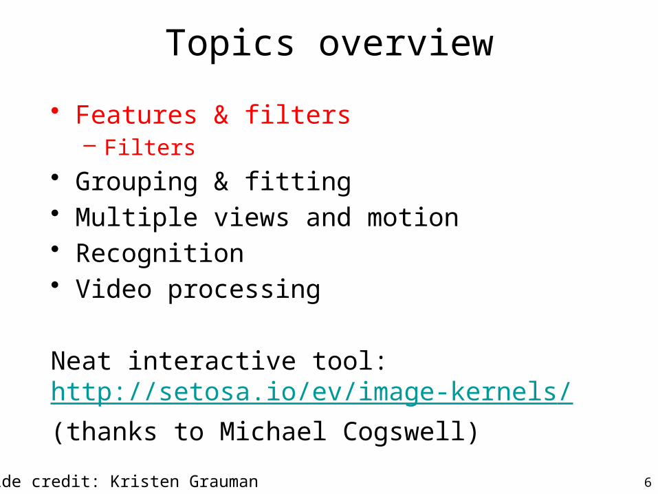
Image filtering
• Compute a function of the local neighborhood at each pixel in the image– Function specified by a “filter” or mask saying how to
combine values from neighbors.
• Uses of filtering:– Enhance an image (denoise, resize, etc)– Extract information (texture, edges, etc)– Detect patterns (template matching)
16Slide credit: Kristen Grauman, Adapted from Derek Hoiem

Motivation: noise reduction
• Even multiple images of the same static scene will not be identical.
17Slide credit: Adapted from Kristen Grauman
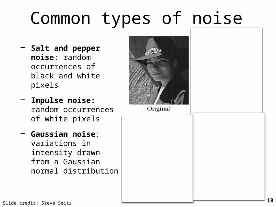
Common types of noise
– Salt and pepper noise: random occurrences of black and white pixels
– Impulse noise: random occurrences of white pixels
– Gaussian noise: variations in intensity drawn from a Gaussian normal distribution
18Slide credit: Steve Seitz

Gaussian noise
>> noise = randn(size(im)).*sigma;>> output = im + noise;
What is impact of the sigma?Slide credit: Kristen GraumanFigure from Martial Hebert 19

Motivation: noise reduction
• Even multiple images of the same static scene will not be identical.
• How could we reduce the noise, i.e., give an estimate of the true intensities?
• What if there’s only one image?
20Slide credit: Kristen Grauman

First attempt at a solution• Let’s replace each pixel with an average of all
the values in its neighborhood• Assumptions:
• Expect pixels to be like their neighbors• Expect noise processes to be independent from pixel to
pixel
21Slide credit: Kristen Grauman

First attempt at a solution• Let’s replace each pixel with an average of all
the values in its neighborhood• Moving average in 1D:
22Slide credit: S. Marschner

Weighted Moving Average
Can add weights to our moving average
Weights [1, 1, 1, 1, 1] / 5
23Slide credit: S. Marschner

Weighted Moving Average
Non-uniform weights [1, 4, 6, 4, 1] / 16
24Slide credit: S. Marschner

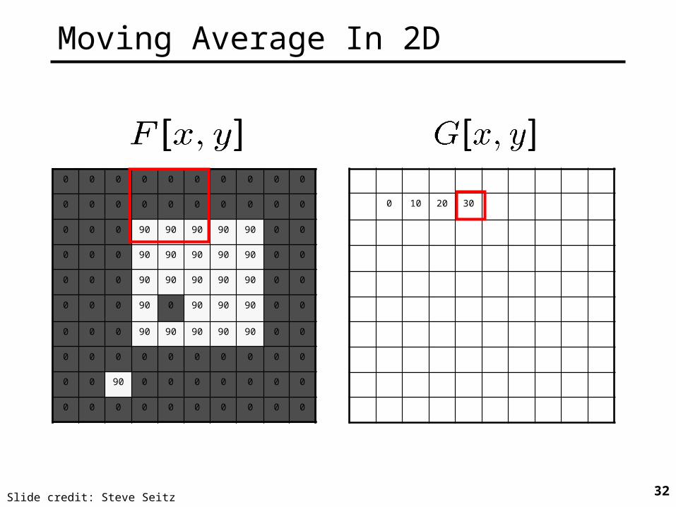
Moving Average In 2D
0 0 0 0 0 0 0 0 0 0
0 0 0 0 0 0 0 0 0 0
0 0 0 90 90 90 90 90 0 0
0 0 0 90 90 90 90 90 0 0
0 0 0 90 90 90 90 90 0 0
0 0 0 90 0 90 90 90 0 0
0 0 0 90 90 90 90 90 0 0
0 0 0 0 0 0 0 0 0 0
0 0 90 0 0 0 0 0 0 0
0 0 0 0 0 0 0 0 0 0
0 0 0 0 0 0 0 0 0 0
0 0 0 0 0 0 0 0 0 0
0 0 0 90 90 90 90 90 0 0
0 0 0 90 90 90 90 90 0 0
0 0 0 90 90 90 90 90 0 0
0 0 0 90 0 90 90 90 0 0
0 0 0 90 90 90 90 90 0 0
0 0 0 0 0 0 0 0 0 0
0 0 90 0 0 0 0 0 0 0
0 0 0 0 0 0 0 0 0 0
25Slide credit: Steve Seitz

Moving Average In 2D
0 0 0 0 0 0 0 0 0 0
0 0 0 0 0 0 0 0 0 0
0 0 0 90 90 90 90 90 0 0
0 0 0 90 90 90 90 90 0 0
0 0 0 90 90 90 90 90 0 0
0 0 0 90 0 90 90 90 0 0
0 0 0 90 90 90 90 90 0 0
0 0 0 0 0 0 0 0 0 0
0 0 90 0 0 0 0 0 0 0
0 0 0 0 0 0 0 0 0 0
0
0 0 0 0 0 0 0 0 0 0
0 0 0 0 0 0 0 0 0 0
0 0 0 90 90 90 90 90 0 0
0 0 0 90 90 90 90 90 0 0
0 0 0 90 90 90 90 90 0 0
0 0 0 90 0 90 90 90 0 0
0 0 0 90 90 90 90 90 0 0
0 0 0 0 0 0 0 0 0 0
0 0 90 0 0 0 0 0 0 0
0 0 0 0 0 0 0 0 0 0
26Slide credit: Steve Seitz

Moving Average In 2D
0 0 0 0 0 0 0 0 0 0
0 0 0 0 0 0 0 0 0 0
0 0 0 90 90 90 90 90 0 0
0 0 0 90 90 90 90 90 0 0
0 0 0 90 90 90 90 90 0 0
0 0 0 90 0 90 90 90 0 0
0 0 0 90 90 90 90 90 0 0
0 0 0 0 0 0 0 0 0 0
0 0 90 0 0 0 0 0 0 0
0 0 0 0 0 0 0 0 0 0
0
0 0 0 0 0 0 0 0 0 0
0 0 0 0 0 0 0 0 0 0
0 0 0 90 90 90 90 90 0 0
0 0 0 90 90 90 90 90 0 0
0 0 0 90 90 90 90 90 0 0
0 0 0 90 0 90 90 90 0 0
0 0 0 90 90 90 90 90 0 0
0 0 0 0 0 0 0 0 0 0
0 0 90 0 0 0 0 0 0 0
0 0 0 0 0 0 0 0 0 0
27Slide credit: Steve Seitz

Moving Average In 2D
0 0 0 0 0 0 0 0 0 0
0 0 0 0 0 0 0 0 0 0
0 0 0 90 90 90 90 90 0 0
0 0 0 90 90 90 90 90 0 0
0 0 0 90 90 90 90 90 0 0
0 0 0 90 0 90 90 90 0 0
0 0 0 90 90 90 90 90 0 0
0 0 0 0 0 0 0 0 0 0
0 0 90 0 0 0 0 0 0 0
0 0 0 0 0 0 0 0 0 0
0 10
0 0 0 0 0 0 0 0 0 0
0 0 0 0 0 0 0 0 0 0
0 0 0 90 90 90 90 90 0 0
0 0 0 90 90 90 90 90 0 0
0 0 0 90 90 90 90 90 0 0
0 0 0 90 0 90 90 90 0 0
0 0 0 90 90 90 90 90 0 0
0 0 0 0 0 0 0 0 0 0
0 0 90 0 0 0 0 0 0 0
0 0 0 0 0 0 0 0 0 0
28Slide credit: Steve Seitz

Moving Average In 2D
0 0 0 0 0 0 0 0 0 0
0 0 0 0 0 0 0 0 0 0
0 0 0 90 90 90 90 90 0 0
0 0 0 90 90 90 90 90 0 0
0 0 0 90 90 90 90 90 0 0
0 0 0 90 0 90 90 90 0 0
0 0 0 90 90 90 90 90 0 0
0 0 0 0 0 0 0 0 0 0
0 0 90 0 0 0 0 0 0 0
0 0 0 0 0 0 0 0 0 0
0 10
0 0 0 0 0 0 0 0 0 0
0 0 0 0 0 0 0 0 0 0
0 0 0 90 90 90 90 90 0 0
0 0 0 90 90 90 90 90 0 0
0 0 0 90 90 90 90 90 0 0
0 0 0 90 0 90 90 90 0 0
0 0 0 90 90 90 90 90 0 0
0 0 0 0 0 0 0 0 0 0
0 0 90 0 0 0 0 0 0 0
0 0 0 0 0 0 0 0 0 0
29Slide credit: Steve Seitz

Moving Average In 2D
0 0 0 0 0 0 0 0 0 0
0 0 0 0 0 0 0 0 0 0
0 0 0 90 90 90 90 90 0 0
0 0 0 90 90 90 90 90 0 0
0 0 0 90 90 90 90 90 0 0
0 0 0 90 0 90 90 90 0 0
0 0 0 90 90 90 90 90 0 0
0 0 0 0 0 0 0 0 0 0
0 0 90 0 0 0 0 0 0 0
0 0 0 0 0 0 0 0 0 0
0 10 20
0 0 0 0 0 0 0 0 0 0
0 0 0 0 0 0 0 0 0 0
0 0 0 90 90 90 90 90 0 0
0 0 0 90 90 90 90 90 0 0
0 0 0 90 90 90 90 90 0 0
0 0 0 90 0 90 90 90 0 0
0 0 0 90 90 90 90 90 0 0
0 0 0 0 0 0 0 0 0 0
0 0 90 0 0 0 0 0 0 0
0 0 0 0 0 0 0 0 0 0
30Slide credit: Steve Seitz

Moving Average In 2D
0 0 0 0 0 0 0 0 0 0
0 0 0 0 0 0 0 0 0 0
0 0 0 90 90 90 90 90 0 0
0 0 0 90 90 90 90 90 0 0
0 0 0 90 90 90 90 90 0 0
0 0 0 90 0 90 90 90 0 0
0 0 0 90 90 90 90 90 0 0
0 0 0 0 0 0 0 0 0 0
0 0 90 0 0 0 0 0 0 0
0 0 0 0 0 0 0 0 0 0
0 10 20
0 0 0 0 0 0 0 0 0 0
0 0 0 0 0 0 0 0 0 0
0 0 0 90 90 90 90 90 0 0
0 0 0 90 90 90 90 90 0 0
0 0 0 90 90 90 90 90 0 0
0 0 0 90 0 90 90 90 0 0
0 0 0 90 90 90 90 90 0 0
0 0 0 0 0 0 0 0 0 0
0 0 90 0 0 0 0 0 0 0
0 0 0 0 0 0 0 0 0 0
31Slide credit: Steve Seitz
Moving Average In 2D
0 0 0 0 0 0 0 0 0 0
0 0 0 0 0 0 0 0 0 0
0 0 0 90 90 90 90 90 0 0
0 0 0 90 90 90 90 90 0 0
0 0 0 90 90 90 90 90 0 0
0 0 0 90 0 90 90 90 0 0
0 0 0 90 90 90 90 90 0 0
0 0 0 0 0 0 0 0 0 0
0 0 90 0 0 0 0 0 0 0
0 0 0 0 0 0 0 0 0 0
0 10 20 30
0 0 0 0 0 0 0 0 0 0
0 0 0 0 0 0 0 0 0 0
0 0 0 90 90 90 90 90 0 0
0 0 0 90 90 90 90 90 0 0
0 0 0 90 90 90 90 90 0 0
0 0 0 90 0 90 90 90 0 0
0 0 0 90 90 90 90 90 0 0
0 0 0 0 0 0 0 0 0 0
0 0 90 0 0 0 0 0 0 0
0 0 0 0 0 0 0 0 0 0
32Slide credit: Steve Seitz
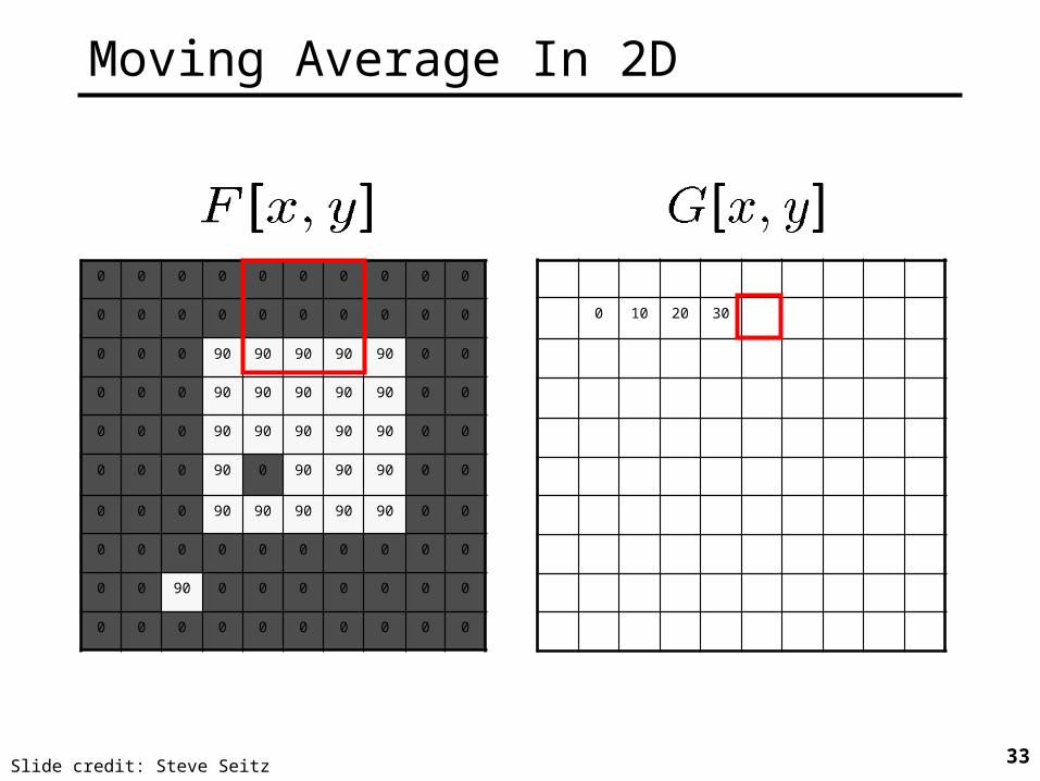
Moving Average In 2D
0 10 20 30
0 0 0 0 0 0 0 0 0 0
0 0 0 0 0 0 0 0 0 0
0 0 0 90 90 90 90 90 0 0
0 0 0 90 90 90 90 90 0 0
0 0 0 90 90 90 90 90 0 0
0 0 0 90 0 90 90 90 0 0
0 0 0 90 90 90 90 90 0 0
0 0 0 0 0 0 0 0 0 0
0 0 90 0 0 0 0 0 0 0
0 0 0 0 0 0 0 0 0 0
33Slide credit: Steve Seitz

Moving Average In 2D
0 10 20 30 30
0 0 0 0 0 0 0 0 0 0
0 0 0 0 0 0 0 0 0 0
0 0 0 90 90 90 90 90 0 0
0 0 0 90 90 90 90 90 0 0
0 0 0 90 90 90 90 90 0 0
0 0 0 90 0 90 90 90 0 0
0 0 0 90 90 90 90 90 0 0
0 0 0 0 0 0 0 0 0 0
0 0 90 0 0 0 0 0 0 0
0 0 0 0 0 0 0 0 0 0
34Slide credit: Steve Seitz

Moving Average In 2D
0 0 0 0 0 0 0 0 0 0
0 0 0 0 0 0 0 0 0 0
0 0 0 90 90 90 90 90 0 0
0 0 0 90 90 90 90 90 0 0
0 0 0 90 90 90 90 90 0 0
0 0 0 90 0 90 90 90 0 0
0 0 0 90 90 90 90 90 0 0
0 0 0 0 0 0 0 0 0 0
0 0 90 0 0 0 0 0 0 0
0 0 0 0 0 0 0 0 0 0
0 10 20 30 30 30 20 10
0 20 40 60 60 60 40 20
0 30 60 90 90 90 60 30
0 30 50 80 80 90 60 30
0 30 50 80 80 90 60 30
0 20 30 50 50 60 40 20
10 20 30 30 30 30 20 10
10 10 10 0 0 0 0 0
35Slide credit: Steve Seitz

Correlation filteringSay the averaging window size is 2k+1 x 2k+1:
Loop over all pixels in neighborhood around image pixel F[i,j]
Attribute uniform weight to each pixel
Now generalize to allow different weights depending on neighboring pixel’s relative position:
Non-uniform weights
36Slide credit: Kristen Grauman

Correlation filtering
Filtering an image: replace each pixel with a linear combination of its neighbors.
The filter “kernel” or “mask” H[u,v] is the prescription for the weights in the linear combination.
This is called cross-correlation, denoted
37Slide credit: Kristen Grauman

Averaging filter• What values belong in the kernel H for the moving
average example?
0 10 20 30 30
0 0 0 0 0 0 0 0 0 0
0 0 0 0 0 0 0 0 0 0
0 0 0 90 90 90 90 90 0 0
0 0 0 90 90 90 90 90 0 0
0 0 0 90 90 90 90 90 0 0
0 0 0 90 0 90 90 90 0 0
0 0 0 90 90 90 90 90 0 0
0 0 0 0 0 0 0 0 0 0
0 0 90 0 0 0 0 0 0 0
0 0 0 0 0 0 0 0 0 0
111
111
111
“box filter”
?
38Slide credit: Kristen Grauman

Smoothing by averagingdepicts box filter: white = high value, black = low value
original filtered
What if the filter size was 5 x 5 instead of 3 x 3?39Slide credit: Kristen Grauman

Boundary issues
What is the size of the output?• MATLAB: output size / “shape” options
• shape = ‘full’: output size is sum of sizes of f and g• shape = ‘same’: output size is same as f• shape = ‘valid’: output size is difference of sizes of f and g
f
gg
gg
full
f
gg
gg
same
f
gg
gg
valid
40Slide credit: Svetlana Lazebnik

Boundary issues
What about near the edge?• the filter window falls off the edge of the image• need to extrapolate• methods:
– clip filter (black)– wrap around– copy edge– reflect across edge
41Slide credit: S. Marschner

Boundary issues
What about near the edge?• the filter window falls off the edge of the image• need to extrapolate• methods (MATLAB):
– clip filter (black): imfilter(f, g, 0)– wrap around: imfilter(f, g, ‘circular’)– copy edge: imfilter(f, g, ‘replicate’)– reflect across edge: imfilter(f, g, ‘symmetric’)
42Slide credit: S. Marschner
Gaussian filter
0 0 0 0 0 0 0 0 0 0
0 0 0 0 0 0 0 0 0 0
0 0 0 90 90 90 90 90 0 0
0 0 0 90 90 90 90 90 0 0
0 0 0 90 90 90 90 90 0 0
0 0 0 90 0 90 90 90 0 0
0 0 0 90 90 90 90 90 0 0
0 0 0 0 0 0 0 0 0 0
0 0 90 0 0 0 0 0 0 0
0 0 0 0 0 0 0 0 0 0
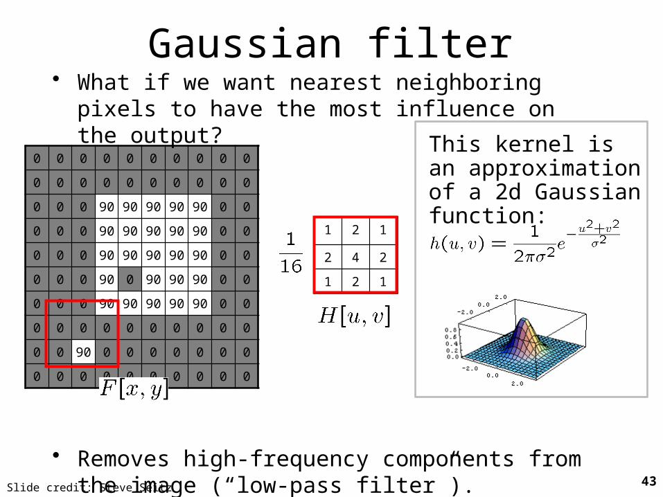
1 2 1
2 4 2
1 2 1
• What if we want nearest neighboring pixels to have the most influence on the output?
• Removes high-frequency components from the image (“low-pass filter”).
This kernel is an approximation of a 2d Gaussian function:
43Slide credit: Steve Seitz

Smoothing with a Gaussian
44Slide credit: Kristen Grauman

Gaussian filters• What parameters matter here?• Size of kernel or mask
– Note, Gaussian function has infinite support, but discrete filters use finite kernels
σ = 5 with 10 x 10 kernel
σ = 5 with 30 x 30 kernel
45Slide credit: Kristen Grauman

Gaussian filters• What parameters matter here?• Variance of Gaussian: determines extent of
smoothing
σ = 2 with 30 x 30 kernel
σ = 5 with 30 x 30 kernel
46Slide credit: Kristen Grauman

Matlab>> hsize = 10;>> sigma = 5;>> h = fspecial(‘gaussian’, hsize, sigma);
>> mesh(h);
>> imagesc(h);
>> outim = imfilter(im, h); % correlation >> imshow(outim);
outim47Slide credit: Kristen Grauman

Smoothing with a Gaussian
for sigma=1:3:10 h = fspecial('gaussian‘, hsize, sigma);out = imfilter(im, h); imshow(out);pause;
end
…
Parameter σ is the “scale” / “width” / “spread” of the Gaussian kernel, and controls the amount of smoothing.
48Slide credit: Kristen Grauman

Properties of smoothing filters
• Smoothing– Values positive – Sum to 1 constant regions same as input– Amount of smoothing proportional to mask size– Remove “high-frequency” components; “low-pass” filter
49Slide credit: Kristen Grauman

Filtering an impulse signal
0 0 0 0 0 0 0
0 0 0 0 0 0 0
0 0 0 0 0 0 0
0 0 0 1 0 0 0
0 0 0 0 0 0 0
0 0 0 0 0 0 0
0 0 0 0 0 0 0
a b c
d e f
g h i
What is the result of filtering the impulse signal (image) F with the arbitrary kernel H?
?
50Slide credit: Kristen Grauman
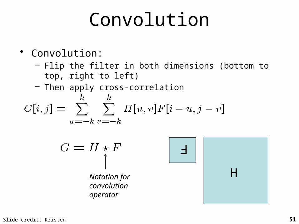
Convolution
• Convolution: – Flip the filter in both dimensions (bottom to top, right to left)– Then apply cross-correlation
Notation for convolution operator
F
H
51Slide credit: Kristen Grauman
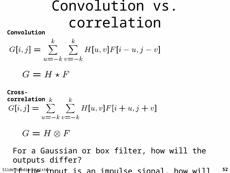
Convolution vs. correlationConvolution
Cross-correlation
For a Gaussian or box filter, how will the outputs differ?
If the input is an impulse signal, how will the outputs differ?52Slide credit: Kristen Grauman

Predict the outputs using correlation filtering
000
010
000
* = ?
000
100
000* = ?
111111111
000020000
-* = ?
53Slide credit: Kristen Grauman

Practice with linear filters
000
010
000
Original
?
54Slide credit: David Lowe

Practice with linear filters
000
010
000
Original Filtered (no change)
55Slide credit: David Lowe

Practice with linear filters
000
100
000
Original
?
56Slide credit: David Lowe

Practice with linear filters
000
100
000
Original Shifted leftby 1 pixel with correlation
57Slide credit: David Lowe

Practice with linear filters
Original
?111
111
111
58Slide credit: David Lowe
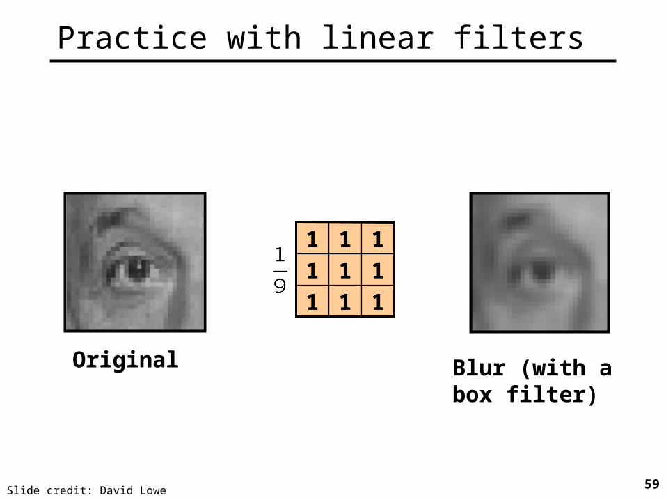
Practice with linear filters
Original
111
111
111
Blur (with abox filter)
59Slide credit: David Lowe
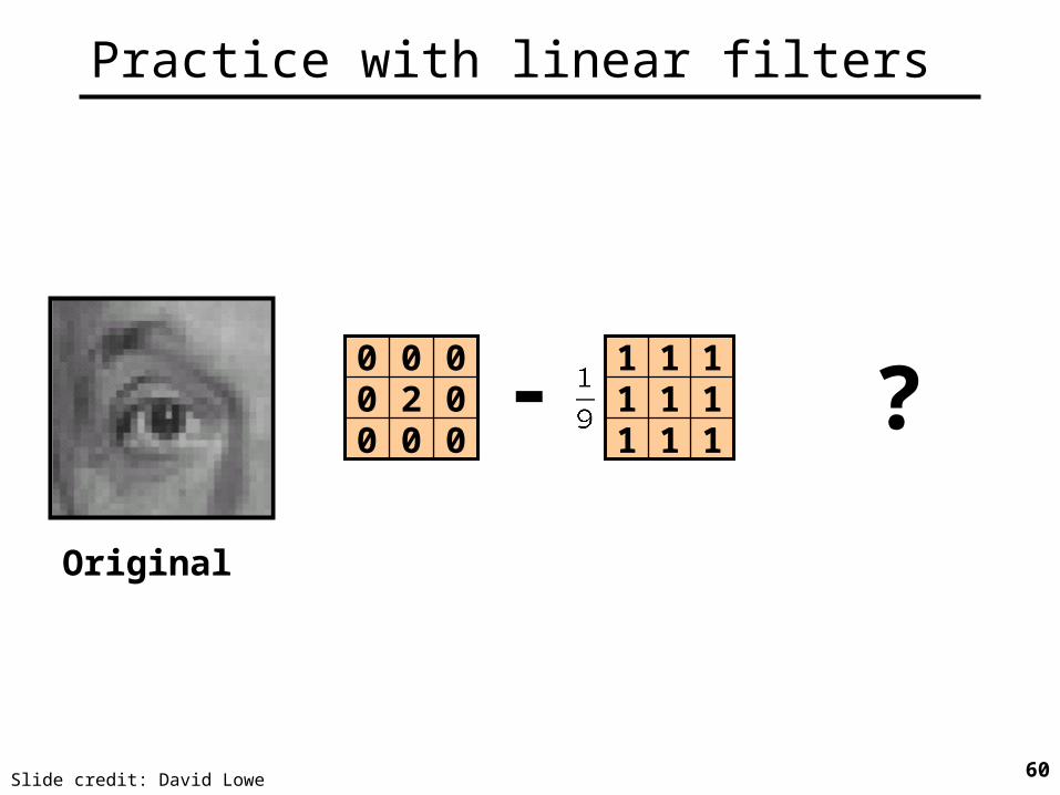
Practice with linear filters
Original
111111111
000020000
- ?
60Slide credit: David Lowe
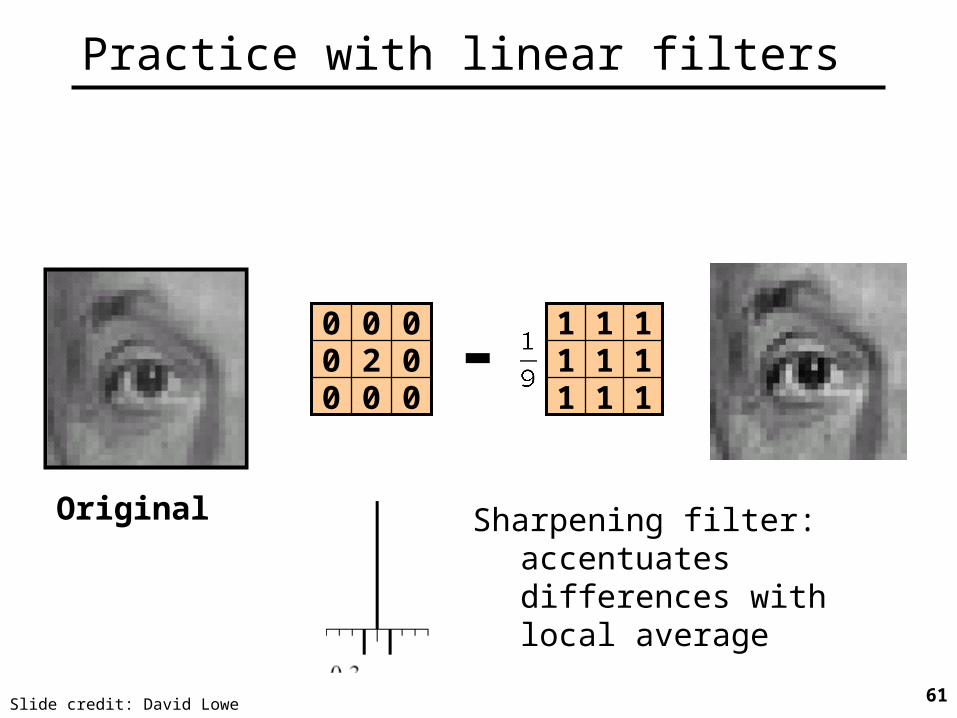
Practice with linear filters
Original
111111111
000020000
-
Sharpening filter:accentuates differences with local average
61Slide credit: David Lowe

Filtering examples: sharpening
62Slide credit: Kristen Grauman
Properties of convolution
• Shift invariant: – Operator behaves the same everywhere, i.e. the
value of the output depends on the pattern in the image neighborhood, not the position of the neighborhood.
• Superposition: – h * (f1 + f2) = (h * f1) + (h * f2)
63Slide credit: Kristen Grauman

Properties of convolution• Commutative:
f * g = g * f
• Associative
(f * g) * h = f * (g * h)
• Distributes over addition
f * (g + h) = (f * g) + (f * h)
• Scalars factor out
kf * g = f * kg = k(f * g)
• Identity:
unit impulse e = […, 0, 0, 1, 0, 0, …]. f * e = f
64Slide credit: Kristen Grauman
Separability• In some cases, filter is separable, and we can factor into
two steps:– Convolve all rows– Convolve all columns
65Slide credit: Kristen Grauman

Separability• In some cases, filter is separable, and we can factor into
two steps: e.g.,
What is the computational complexity advantage for a separable filter of size k x k,
in terms of number of operations per output pixel?
f * (g * h) = (f * g) * h
g
h
f
66Slide credit: Kristen Grauman

Effect of smoothing filters
Additive Gaussian noise Salt and pepper noise
67Slide credit: Kristen Grauman

Median filter
• No new pixel values introduced
• Removes spikes: good for impulse, salt & pepper noise
• Non-linear filter
68Slide credit: Kristen Grauman

Median filter
Salt and pepper noise
Median filtered
Plots of a row of the image
Matlab: output im = medfilt2(im, [h w]);69Slide credit: Martial Hebert

Median filter• Median filter is edge preserving
70Slide credit: Kristen Grauman

Aude Oliva & Antonio Torralba & Philippe G Schyns, SIGGRAPH 2006
Filtering application: Hybrid Images
71Slide credit: Kristen Grauman

Application: Hybrid ImagesGaussian Filter
Laplacian Filter
Gaussianunit impulse Laplacian of Gaussian
72Slide credit: Kristen Grauman
A. Oliva, A. Torralba, P.G. Schyns, “Hybrid Images,” SIGGRAPH 2006

Aude Oliva & Antonio Torralba & Philippe G Schyns, SIGGRAPH 2006 73Slide credit: Kristen Grauman

Aude Oliva & Antonio Torralba & Philippe G Schyns, SIGGRAPH 2006 74Slide credit: Kristen Grauman

Summary
• Image formation• Image “noise”• Linear filters and convolution useful for
– Enhancing images (smoothing, removing noise)• Box filter• Gaussian filter• Impact of scale / width of smoothing filter
– Detecting features (next time)
• Separable filters more efficient • Median filter: a non-linear filter, edge-preserving
75Slide credit: Kristen Grauman

Coming up
• Monday night:– PS0 is due via scholar, 11:55 PM
• Tuesday:– Filtering part 2: filtering for features
76

77
Topics overview
• Features & filters– Filters– Gradients– Edges
• Grouping & fitting• Multiple views and motion• Recognition• Video processing
Slide credit: Kristen Grauman

Questions?
See you Tuesday!