Embed Size (px)
Citation preview

1
1.2
© 2012 Pearson Education, Inc.
Linear Equations
in Linear Algebra
Row Reduction and Echelon
Forms

Slide 1.2- 2© 2012 Pearson Education, Inc.
ECHELON FORM
A rectangular matrix is in echelon form (or row
echelon form) if it has the following three
properties:
1. All nonzero rows are above any rows of all
zeros.
2. Each leading entry of a row is in a column to
the right of the leading entry of the row above
it.
3. All entries in a column below a leading entry
are zeros.

Slide 1.2- 3© 2012 Pearson Education, Inc.
ECHELON FORM
If a matrix in echelon form satisfies the following
additional conditions, then it is in reduced echelon
form (or reduced row echelon form):
4. The leading entry in each nonzero row is 1.
5. Each leading 1 is the only nonzero entry in its
column.
An echelon matrix (respectively, reduced echelon
matrix) is one that is in echelon form (respectively,
reduced echelon form.)

Slide 1.2- 4© 2012 Pearson Education, Inc.
ECHELON FORM
Any nonzero matrix may be row reduced (i.e.,
transformed by elementary row operations) into more
than one matrix in echelon form, using different
sequences of row operations. However, the reduced
echelon form one obtains from a matrix is unique.
Theorem 1: Uniqueness of the Reduced Echelon
Form
Each matrix is row equivalent to one and only one
reduced echelon matrix.

Slide 1.2- 5© 2012 Pearson Education, Inc.
PIVOT POSITION
If a matrix A is row equivalent to an echelon matrix
U, we call U an echelon form (or row echelon form)
of A; if U is in reduced echelon form, we call U the
reduced echelon form of A.
A pivot position in a matrix A is a location in A that
corresponds to a leading 1 in the reduced echelon
form of A. A pivot column is a column of A that
contains a pivot position.

Slide 1.2- 6© 2012 Pearson Education, Inc.
PIVOT POSITION
Example 1: Row reduce the matrix A below to echelon form, and locate the pivot columns of A.
Solution: The top of the leftmost nonzero column is the first pivot position. A nonzero entry, or pivot, must be placed in this position.
0 3 6 4 9
1 2 1 3 1
2 3 0 3 1
1 4 5 9 7
A

Slide 1.2- 7© 2012 Pearson Education, Inc.
PIVOT POSITION
Now, interchange rows 1 and 4.
Create zeros below the pivot, 1, by adding multiples of the first row to the rows below, and obtain the next matrix.
1 4 5 9 7
1 2 1 3 1
2 3 0 3 1
0 3 6 4 9
Pivot
Pivot column
Slide 1.2- 8© 2012 Pearson Education, Inc.
PIVOT POSITION
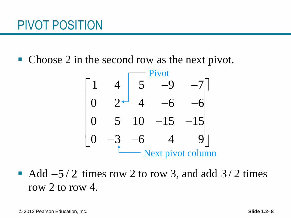
Choose 2 in the second row as the next pivot.
Add times row 2 to row 3, and add times
row 2 to row 4.
1 4 5 9 7
0 2 4 6 6
0 5 10 15 15
0 3 6 4 9
Pivot
Next pivot column
5 / 2 3 / 2

Slide 1.2- 9© 2012 Pearson Education, Inc.
PIVOT POSITION
There is no way a leading entry can be created in
column 3. But, if we interchange rows 3 and 4, we
can produce a leading entry in column 4.
1 4 5 9 7
0 2 4 6 6
0 0 0 0 0
0 0 0 5 0

Slide 1.2- 10© 2012 Pearson Education, Inc.
PIVOT POSITION
1 4 5 9 7
0 2 4 6 6
0 0 0 5 0
0 0 0 0 0
The matrix is in echelon form and thus reveals that
columns 1, 2, and 4 of A are pivot columns.
Pivot
Pivot columns
Slide 1.2- 11© 2012 Pearson Education, Inc.
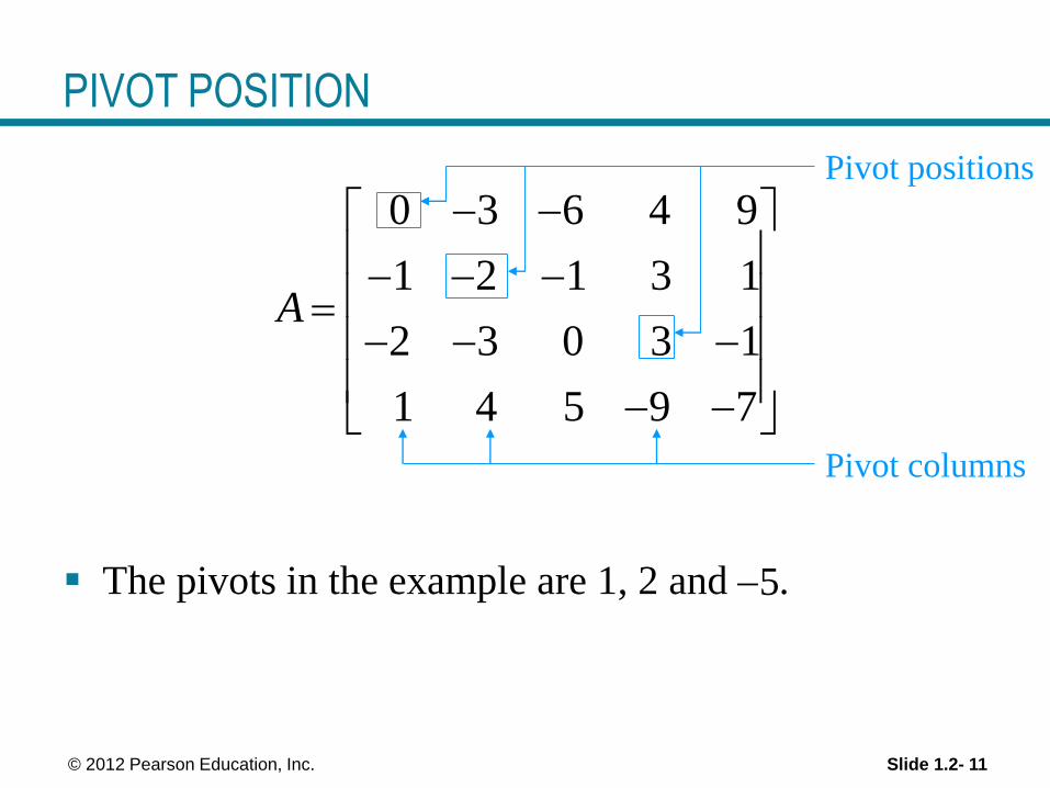
PIVOT POSITION
0 3 6 4 9
1 2 1 3 1
2 3 0 3 1
1 4 5 9 7
A
The pivots in the example are 1, 2 and .
Pivot positions
Pivot columns
5

Slide 1.2- 12© 2012 Pearson Education, Inc.
ROW REDUCTION ALGORITHM
Example 2: Apply elementary row operations to transform the following matrix first into echelon form and then into reduced echelon form.
Solution:
STEP 1: Begin with the leftmost nonzero column. This is a pivot column. The pivot position is at the top.
0 3 6 6 4 5
3 7 8 5 8 9
3 9 12 9 6 15
Slide 1.2- 13© 2012 Pearson Education, Inc.
ROW REDUCTION ALGORITHM
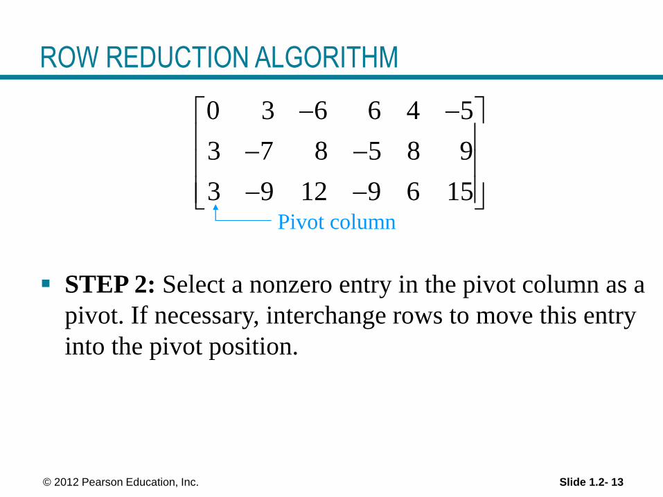
STEP 2: Select a nonzero entry in the pivot column as a
pivot. If necessary, interchange rows to move this entry
into the pivot position.
0 3 6 6 4 5
3 7 8 5 8 9
3 9 12 9 6 15
Pivot column

Slide 1.2- 14© 2012 Pearson Education, Inc.
ROW REDUCTION ALGORITHM
Interchange rows 1 and 3. (Rows 1 and 2 could have
also been interchanged instead.)
STEP 3: Use row replacement operations to create
zeros in all positions below the pivot.
3 9 12 9 6 15
3 7 8 5 8 9
0 3 6 6 4 5
Pivot

Slide 1.2- 15© 2012 Pearson Education, Inc.
ROW REDUCTION ALGORITHM
We could have divided the top row by the pivot, 3, but
with two 3s in column 1, it is just as easy to add
times row 1 to row 2.
STEP 4: Cover the row containing the pivot position,
and cover all rows, if any, above it. Apply steps 1–3 to
the submatrix that remains. Repeat the process until
there are no more nonzero rows to modify.
1
3 9 12 9 6 15
0 2 4 4 2 6
0 3 6 6 4 5
Pivot

Slide 1.2- 16© 2012 Pearson Education, Inc.
ROW REDUCTION ALGORITHM
With row 1 covered, step 1 shows that column 2 is the
next pivot column; for step 2, select as a pivot the “top”
entry in that column.
For step 3, we could insert an optional step of dividing
the “top” row of the submatrix by the pivot, 2. Instead,
we add times the “top” row to the row below.
3 9 12 9 6 15
0 2 4 4 2 6
0 3 6 6 4 5
Pivot
New pivot column
3 / 2

Slide 1.2- 17© 2012 Pearson Education, Inc.
ROW REDUCTION ALGORITHM
This produces the following matrix.
When we cover the row containing the second pivot
position for step 4, we are left with a new submatrix that
has only one row.
3 9 12 9 6 15
0 2 4 4 2 6
0 0 0 0 1 4
3 9 12 9 6 15
0 2 4 4 2 6
0 0 0 0 1 4

Slide 1.2- 18© 2012 Pearson Education, Inc.
ROW REDUCTION ALGORITHM
Steps 1–3 require no work for this submatrix, and we
have reached an echelon form of the full matrix. We
perform one more step to obtain the reduced echelon
form.
STEP 5: Beginning with the rightmost pivot and
working upward and to the left, create zeros above
each pivot. If a pivot is not 1, make it 1 by a scaling
operation.
The rightmost pivot is in row 3. Create zeros above it,
adding suitable multiples of row 3 to rows 2 and 1.
Slide 1.2- 19© 2012 Pearson Education, Inc.
ROW REDUCTION ALGORITHM
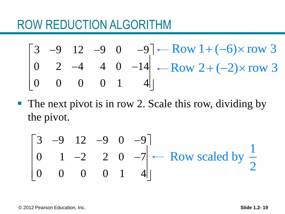
3 9 12 9 0 9
0 2 4 4 0 14
0 0 0 0 1 4
The next pivot is in row 2. Scale this row, dividing by
the pivot.
Row 1 ( 6) row 3
Row 2 ( 2) row 3
3 9 12 9 0 9
0 1 2 2 0 7
0 0 0 0 1 4
1Row scaled by
2

Slide 1.2- 20© 2012 Pearson Education, Inc.
ROW REDUCTION ALGORITHM
Create a zero in column 2 by adding 9 times row 2 to
row 1.
Finally, scale row 1, dividing by the pivot, 3.
Row 1 (9) row 2 3 0 6 9 0 72
0 1 2 2 0 7
0 0 0 0 1 4
Slide 1.2- 21© 2012 Pearson Education, Inc.
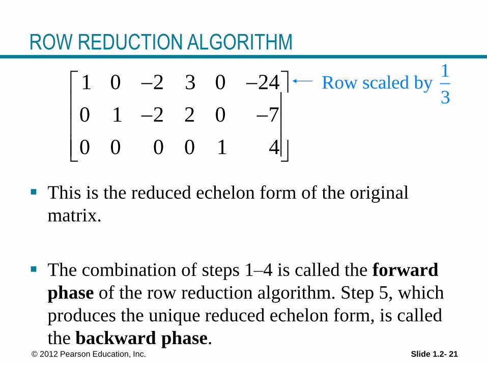
ROW REDUCTION ALGORITHM
This is the reduced echelon form of the original
matrix.
The combination of steps 1–4 is called the forward
phase of the row reduction algorithm. Step 5, which
produces the unique reduced echelon form, is called
the backward phase.
1 0 2 3 0 24
0 1 2 2 0 7
0 0 0 0 1 4
1Row scaled by
3

Slide 1.2- 22© 2012 Pearson Education, Inc.
SOLUTIONS OF LINEAR SYSTEMS
The row reduction algorithm leads to an explicit
description of the solution set of a linear system when
the algorithm is applied to the augmented matrix of
the system.
Suppose that the augmented matrix of a linear system
has been changed into the equivalent reduced echelon
form.1 0 5 1
0 1 1 4
0 0 0 0
Slide 1.2- 23© 2012 Pearson Education, Inc.
SOLUTIONS OF LINEAR SYSTEMS
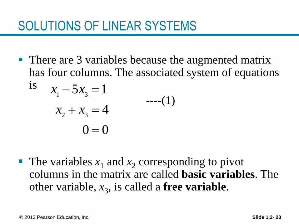
There are 3 variables because the augmented matrix has four columns. The associated system of equations is
----(1)
The variables x1 and x2 corresponding to pivot columns in the matrix are called basic variables. The other variable, x3, is called a free variable.
1 3
2 3
5 1
4
0 0
x x
x x

Slide 1.2- 24© 2012 Pearson Education, Inc.
SOLUTIONS OF LINEAR SYSTEMS
Whenever a system is consistent, as in (1), the solution set can be described explicitly by solving the reduced system of equations for the basic variables in terms of the free variables.
This operation is possible because the reduced echelon form places each basic variable in one and only one equation.
In (1), solve the first and second equations for x1 and x2. (Ignore the third equation; it offers no restriction on the variables.)
Slide 1.2- 25© 2012 Pearson Education, Inc.
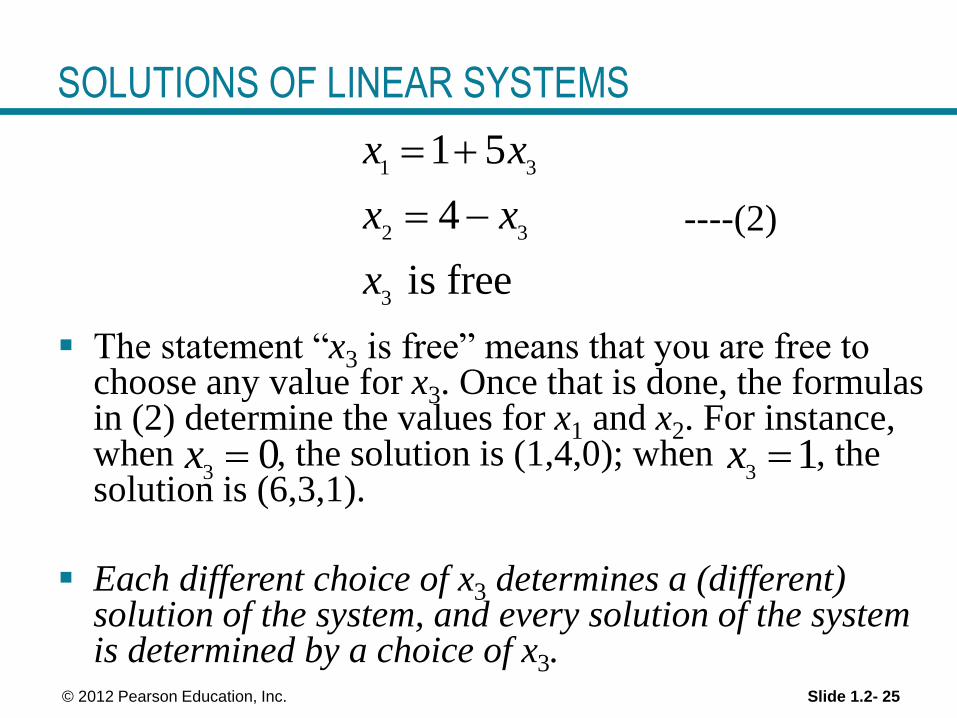
SOLUTIONS OF LINEAR SYSTEMS
----(2)
The statement “x3 is free” means that you are free to choose any value for x3. Once that is done, the formulas in (2) determine the values for x1 and x2. For instance, when , the solution is (1,4,0); when , the solution is (6,3,1).
Each different choice of x3 determines a (different) solution of the system, and every solution of the system is determined by a choice of x3.
30x
31x
1 3
2 3
3
1 5
4
is free
x x
x x
x

Slide 1.2- 26© 2012 Pearson Education, Inc.
PARAMETRIC DESCRIPTIONS OF SOLUTION
SETS
The description in (2) is a parametric description of
solutions sets in which the free variables act as
parameters.
Solving a system amounts to finding a parametric
description of the solution set or determining that the
solution set is empty.
Whenever a system is consistent and has free
variables, the solution set has many parametric
descriptions.

Slide 1.2- 27© 2012 Pearson Education, Inc.
PARAMETRIC DESCRIPTIONS OF SOLUTION
SETS
For instance, in system (1), add 5 times equation 2 to equation 1 and obtain the following equivalent system.
We could treat x2 as a parameter and solve for x1 and x3 in terms of x2, and we would have an accurate description of the solution set.
When a system is inconsistent, the solution set is empty, even when the system has free variables. In this case, the solution set has no parametric representation.
1 2
2 3
5 21
4
x x
x x

Slide 1.2- 28© 2012 Pearson Education, Inc.
EXISTENCE AND UNIQUENESS THEOREM
Theorem 2: Existence and Uniqueness Theorem
A linear system is consistent if and only if the rightmost column of the augmented matrix is not a pivot column—i.e., if and only if an echelon form of the augmented matrix has no row of the form
[0 … 0 b] with b nonzero.
If a linear system is consistent, then the solution set contains either (i) a unique solution, when there are no free variables, or (ii) infinitely many solutions, when there is at least on free variable.

Slide 1.2- 29© 2012 Pearson Education, Inc.
ROW REDUCTION TO SOLVE A LINEAR SYSTEM
Using Row Reduction to Solve a Linear System
1. Write the augmented matrix of the system.
2. Use the row reduction algorithm to obtain an equivalent augmented matrix in echelon form. Decide whether the system is consistent. If there is no solution, stop; otherwise, go to the next step.
3. Continue row reduction to obtain the reduced echelon form.
4. Write the system of equations corresponding to the matrix obtained in step 3.

Slide 1.2- 30© 2012 Pearson Education, Inc.
ROW REDUCTION TO SOLVE A LINEAR SYSTEM
5. Rewrite each nonzero equation from step 4 so
that its one basic variable is expressed in terms of
any free variables appearing in the equation.