Linear Contact Analysis: Demystified · PDF filewith Femap V10.1.1 and Nastran 7.0 Adrian Jensen. ... error. Start to create you ... select a Connection Property from the drop- down

2010 – All Rights Reserved

1 / 26

Linear Contact Analysis: Demystified

with Femap V10.1.1 and Nastran 7.0

Adrian JensenMechanical Engineer

[email protected]


2 / 26Linear Contact Analysis: Demystified

Table of Contents

1. Introduction . . . . . . . . . . . . . . . . . . . . . . . . . . . . . . . . . . . . . . . . . . . . . . . . . . . . . . . 3 2. Regions . . . . . . . . . . . . . . . . . . . . . . . . . . . . . . . . . . . . . . . . . . . . . . . . . . . . . . . . . . 4

a) Solids . . . . . . . . . . . . . . . . . . . . . . . . . . . . . . . . . . . . . . . . . . . . . . . . . . . . . . . 4i. By Surfaces . . . . . . . . . . . . . . . . . . . . . . . . . . . . . . . . . . . . . . . . . . . . . . . 4ii. By Elements . . . . . . . . . . . . . . . . . . . . . . . . . . . . . . . . . . . . . . . . . . . . . . . 5

b) Plates . . . . . . . . . . . . . . . . . . . . . . . . . . . . . . . . . . . . . . . . . . . . . . . . . . . . . . 9i. By Surfaces . . . . . . . . . . . . . . . . . . . . . . . . . . . . . . . . . . . . . . . . . . . . . . . 9ii. By Elements . . . . . . . . . . . . . . . . . . . . . . . . . . . . . . . . . . . . . . . . . . . . . . 10

3. Connectors . . . . . . . . . . . . . . . . . . . . . . . . . . . . . . . . . . . . . . . . . . . . . . . . . . . . . . . 12a) Source-Target . . . . . . . . . . . . . . . . . . . . . . . . . . . . . . . . . . . . . . . . . . . . . . . . . 13

4. Properties. . . . . . . . . . . . . . . . . . . . . . . . . . . . . . . . . . . . . . . . . . . . . . . . . . . . . . . . 15a) Friction . . . . . . . . . . . . . . . . . . . . . . . . . . . . . . . . . . . . . . . . . . . . . . . . . . . . . 16b) Contact Search Distance . . . . . . . . . . . . . . . . . . . . . . . . . . . . . . . . . . . . . . . . . . . 16c) Initial Penetration . . . . . . . . . . . . . . . . . . . . . . . . . . . . . . . . . . . . . . . . . . . . . . . 17d) Shell Offset . . . . . . . . . . . . . . . . . . . . . . . . . . . . . . . . . . . . . . . . . . . . . . . . . . . 18e) Shell Z Offset . . . . . . . . . . . . . . . . . . . . . . . . . . . . . . . . . . . . . . . . . . . . . . . . . . 19f) Refinement. . . . . . . . . . . . . . . . . . . . . . . . . . . . . . . . . . . . . . . . . . . . . . . . . . . 22 g) Penalty Factor . . . . . . . . . . . . . . . . . . . . . . . . . . . . . . . . . . . . . . . . . . . . . . . . . 24



Introduction

Frustrated?Using linear contact can be frustrating. In fact, it is probably one of the most frequent subjects of calls for tech support staff. But when you break it down into its most simple components, it doesn’t have to be frustrating. It can be a quick, easy and usefultechnique in your FEA toolbox. It all boils down to element faces intersecting other element faces. If you correctly specify thecontact regions and the initial contact conditions you will have success with linear contact analysis.

What is linear contact?Linear contact is called such because there is no geometric or material non-linearity in the analysis. That is, the stiffness matrix is not updated and the material behaves in a linear elastic fashion. Take for example a small steel punch pressing against a surface. Let’s assume a nominal elastic modulus of 29,000,000 psi and a yield strength of 60,000 psi. When the steel reaches the yieldstress, it has a strain of 0.2% (60,000 psi / 29,000,000 psi). If that punch was originally 1” long, it has compressed 0.002”. One could safely assume that the behavior of the system has changed very little. What does this all mean? For problems with stiffengineering materials (e.g. steel) where the material is not stressed beyond the yield strength, linear contact is a reasonable analysis mechanism.

How does it work?This white paper will cover a wide range of linear contact problems from the simple task of setting up contact regions to the more daunting charge of manually adjusting the penalty factors. The key to any linear contact problem it to start simple. Before you try to run that 500,000 node model with 20 contact regions, build small, manageable models of the different contact scenarios foreasy debugging.



Connection RegionsWhen you break a linear contact problem down into its most simple component, you have a Connection Region. It might seem like an elementary step in the analysis but if it is not done correctly, there will be problems that can’t be fixed by toying with the more advanced components of linear contact.

Connection Regions: Solids, by SurfacesThe easiest linear contact analysis to set up is for a simple solid model using surfaces. When creating your Connection Region by surfaces you’ll notice an option to select the positive or negative. For solid models, this option is not necessary. If you check the normals of the surfaces of the solid body, they’re all facing outward. The option to modify surface normals only works for sheetsolids. Additionally, even if you do select the negative face of a surface, your results will change negligibly.



Connection Regions: Solids, by ElementsIn some cases you be unable to select your Connection Regions by surfaces. The other option is to select your regions by elements. This technique gives you more control over selecting your Connection Region, but also opens up the possibility for error. Start to create you Connection Region by selecting the “Elements” radio button under the “Defined By” section of the Connection Region dialogue box.

Assuming you don’t want to select elements one-by-one, click the “Multiple” button. There are two stages to the region selectionby elements: the element selection and the element face selection. The element selection is simple; grab all elements that have faces you want to include in the Connection Region.



Regions: Solids, by ElementsThe element face selection is a bit trickier. Once you have selected the elements you want, you are presented five options for face selection. The following pages provides examples of each.

Face ID: Each face of an element has a face id. Plate elements use faces 1 & 2, tet elements use faces 1-4 and hex elements use faces 1-6. This option is generally the least useful for a solid model because the element faces on the surface of the solid do not necessarily share a common face ID. The graphics below show the Connection Regions created by selecting all of the elements and using the“Face ID” face selection method. The first graphic shows face 1, the second shows face 2 and so forth.



Connection Regions: Solids, by ElementsNear Surface:This option is useful if you have geometry to work with but you don’t want to limit the elements in your Connection Region. The graphics below show the Connection Regions created by selecting a cluster of elements in the corner of the block and using the “Near Surface” face selection method.

Near Coordinates:The “Near Coordinates” method is very similar to “Near Surface”. Instead of specifying a surface, however, you choose a coordinate system, direction and position. This defines a planar surface, which is used along with the tolerance to find the closest faces.



Connection Regions: Solids, by ElementsAdjacent Faces:A powerful method for choosing faces, especially for complex solid and planar element models. You choose just one initial face (and the associated element ID). This can be done very easily by graphically selecting the face. You then specify a tolerance angle. FEMAP will search all selected elements for faces that are connected to the face that you chose and that are within the specified tolerance from being coplanar with an already selected face.

Model Free FacesThe “Model Free Faces” method simply includes every "free element face" in your element selection. A good technique if you can grab exactly the elements you want within the element selection dialogue box.



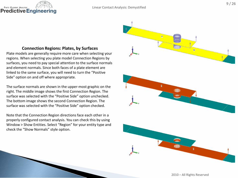
Connection Regions: Plates, by SurfacesPlate models are generally require more care when selecting your regions. When selecting you plate model Connection Regions by surfaces, you need to pay special attention to the surface normals and element normals. Since both faces of a plate element are linked to the same surface, you will need to turn the “Positive Side” option on and off where appropriate.

The surface normals are shown in the upper-most graphic on the right. The middle image shows the first Connection Region. The surface was selected with the “Positive Side” option unchecked. The bottom image shows the second Connection Region. The surface was selected with the “Positive Side” option checked.

Note that the Connection Region directions face each other in a properly configured contact analysis. You can check this by using Window > Show Entities. Select “Region” for your entity type and check the “Show Normals” style option.



Connection Regions: Plates, by ElementsIn some cases you be unable to select your Connection Regions by surfaces. The other option is to select your regions by elements. This technique gives you more control over selecting your Connection Region, but also opens up the possibility for error. Start to create you Connection Region by selecting the “Elements” radio button under the “Defined By” section of the Connection Region dialogue box. You probably don’t want to select elements one-by-one. Use the “Multiple” button to speed things up.



Regions: Plates, by ElementsOnce you have selected the elements you want, you are presented five options for face selection. When working with plate elements, only the “Face ID” and “Adjacent Faces” options should be used.

Face ID: As mentioned earlier, plate elements use faces 1 & 2 for Connection Regions. Be aware that a four sided plate element has sixfaces and Femap will allow you to select any of these faces but only faces 1 & 2 are supported for contact. The “Face ID” methodallows you to enter the face ID numerically or select a face from the model. This model is more effective with plate models because the faces of the elements are more commonly aligned.

Adjacent Faces:This method is useful for creating Connection Regions when elements do not have consistent orientation or when the model has complex geometry (see “Adjacent Faces” in the solid element section).

Hint: Turn on element thickness to help you check the Connection Region you have created.



ConnectorsOnce you have properly set up your Connection Regions, you must establish contact pairs, called “Connectors” in the Femap interface. A Connector specifies a contact mechanism in the model with a “Source” Connection Region, a “Target” Connection Region and a Connection Property.

Setting up a Connector is quite simple, select a Connection Property from the drop-down list or use the quick button to the right to create a new one. Leave the fields of the Connection Property blank for now. Connection Properties will be discussed in greater detail later in this white paper. Next, select Master (Target) and Slave (Source) Connection Regions from the drop-down lists orselect by clicking on the desired Connection Regions in the model. The Connection Regions will highlight as you place the cursorover them to make the selection process easier (see the graphic above).



Connectors: Source Regions and Target Regions, from the NX Nastran 7 User’s GuideIt's important to understand how contact element are created when selecting which region will be the source and which the target, since the two can be interchangeable. The solver projects vector normals from the source region to the target region. Itthen creates contact elements when these normals intersect elements in the target region and are within the search distance criteria for the contact pair. This means that when the two regions of a pair do not have corresponding one-to-one elements, thenumber of contact elements that the solver creates can change depending on which region it projects the elements from and which region it projects them to.

In general, of the two contact regions you use for the pair, choose the one with the finer mesh for the source region. When the source and target regions have different mesh densities, more elements on the source region will mean that more contact elements are created, which will produce a more accurate solution.

For example, the two regions below are both composed of linear shells. The source region (A) has one element and the target region (B) has four elements.

When creating the contact elements between these regions, the software projects contact elements from the single element on the source region to the four elements in the target region. This results in the creation of a single contact element (see the graphic on the left).

However, if you were to use the region with four elements as the source (C) and the region with one element as the target (D), the solution will create 4 contact elements (see the graphic on the right).



Connectors: Source Regions and Target Regions, from the NX Nastran 7 User’s GuideIn the example below, both the sphere and the rectangular plate were meshed with plate elements. The sphere has a higher meshdensity. The edges of the rectangle are fixed and the sphere is pushed downward into the plate.

In the graphics below, the sphere is viewed from the bottom with contact pressure contoured over the model. In the graphic onthe left, the Connector was setup with the sphere as the Source Region and the rectangular plate as the Target Region. As predicted, a single hot spot is present at the bottom-center of the sphere. In the graphic on the right, the Connector was setupwith the rectangular plate as the Source Region and the sphere as the Target Region. Four separate hot spots are present, each covering four corners of an element. This result set is clearly incorrect and is caused by a lack of contact elements created for the analysis.



Connection PropertiesAfter you have created and checked your Connection Regions and Connectors you can set up the Connection Property.

Although a Connection Property is required to create a Connector, it is recommended that fully configuring the Connection Property should be saved for last. This is because it is easy to get overwhelmed with the options provided on a Connection Property card. Additionally, unless the Connection Regions and Connectors are configured correctly, none of the options of the Connection Property will allow for a accurate contact analysis.

The Connection Property card is divided into three sections: Contact Pair (BCTSET), Contact Property (BCTPARAM) and Common Contact Parameters (BCTPARAM). Common Glue Parameters (BGPARAM) and Glued Contact Property (BGSET) will not be covered in this white paper.



Connection Properties: Contact Pair (BCTSET)The options in this portion of the dialog box can be set individually for each Connector (contact pair) that is created in the model. These options will be written out to the BCTSET entry for each individual contact pair. Each contact pair will be designated in the graphics window with a single line going from one Connection Region to another and this line is a contact element.

Min Contact Search Dist/Max Contact Search Dist – As discussed in the Connectors section, contact elements are created when these normals projected from the source region intersect elements in the target region within the search distance. The search distance is specified with Min Contact Search Dist and Max Contact Search Dist.Note: The minimum distance can be negative and used for an interference fit condition modeled as overlapping surfaces.

Friction – The static coefficient of friction for the contact pair. For many contact analyses it is important to include a Friction value to provide stability to the model. For example, in the image below, a small, arbitrary Friction value was used to constrain the inner tube from translating in the Z direction.

Note: In general, if different friction values are NOT needed then the contact pairs should all reference the same contact property.



Connection Properties: Contact Property (BCTPARM) Initial Penetration - Controls how Nastran handles initial gap or penetration of the generated contact elements. This setting is particularly useful if some of your elements unintentionally penetrate each other and you do not wish to modify or rebuild your model. 0..Calculated - Use the value calculated from the grid coordinates. In the case of penetrations, a model may experience "press fit" behavior when using this option.2..Calculated/Zero Penetrations - Same as 0..Calculated, but if penetration is detected, set the value to zero.3..Zero Gap/Penetration - Sets the penetration/gap to zero for all contact elements.



Connection Properties: Contact Property (BCTPARM) Shell Offset – For plate elements, you can enforce contact at either the midplane or the surface. This option, as well as the Initial Penetration option, can save modeling time when optimizing a plate thickness of a component in a contact region. The gap between connection regions will be independent of plate element thickness if this option is turned off.0..Include shell thickness - Include half shell thickness as surface offset.1..Do not include thickness - Does not include thickness offset.

The images on the left show results with Shell Offset turned off and the images to the right show results with the Shell Offset option turned on. The models are displayed with and without thickness on top and bottom respectively.



Connection Properties: Contact Property (BCTPARM) Shell Z-Offset - Allows you to choose if the Z-Offset on shell elements should be included in the contact analysis. 0..Include Z-Offset (Default) - Z offset of shells is included as surface offset.1..No not Include Z-Offset - Z offset of shells is NOT included as surface offset.

The images on the left show results with Shell Z Offset turned off and the images to the right show results with the Shell Z Offset option turned on. The models are displayed with and without element offsets on top and bottom respectively.



Connection Properties: Contact Property (BCTPARM) These options need to only be defined once for a contact analysis, regardless of how many Connectors (contact pairs) are defined in the model. Each Connector has an ID assigned to it and can reference a different Connection Property. FEMAP will use the Connection Property referenced by the Connector with the lowest ID to define the BCTPARM entry for the entire model. For example, if a model has 2 Connectors (contact pairs) with ID numbers 101 and 102, the Connection Property values defined in the property associated with Connector ID 101 would be used for the analysis.

Max Force Iterations - Creates the MAXF field on the BCTPARM entry. Designates the maximum number of iterations for a force (inner) loop (Default = 10).

Max Status Iterations - Creates the MAXS field on the BCTPARM entry. Designates the maximum number of iterations for a status (outer) loop (Default = 20).

Force Convergence Tol - Creates the CTOL field on the BCTPARM entry. Designates the Contact Force convergence tolerance (Default = 0.01). Convergence Criteria and Num For Convergence - Together, these two values create the NCHG field on the BCTPARM entry. The value and type of number (real or integer) entered for Num For Convergence depends on the option set for Convergence Criteria: 0..Number of Changes - When this option is set, Num for Convergence must be an integer > 1. This value defines the allowable number of contact changes.1..Percentage of Active - When this option is set, Num for Convergence must be entered as a percentage (between 1 and 99, which will appear as 0.01 to 0.99 in the NX Nastran input file). The solver treats this value as a percentage of the number of active contact elements in each outer loop of the contact algorithm. The number of active contact elements is evaluated at each outer loop iteration.

Min Contact Percentage - Creates the MPER field on the BCTPARM entry. Designates the Minimum Contact Set Percentage (Default = 100).



Connection Properties: Contact Property (BCTPARM)

Adaptive Stiffness - This is a flag to indicate whether adaptive stiffness is activated. Creates PENADAPT field on BCTPARM entry (Default=0). When not checked, it places a "0" (No Adaptive adjustment) into the PENADAPT field, when checked places a "1" (Adaptively adjusts contact stiffness) into the PENADAPT field.

Penetration Factor - Creates the PENETFAC field on the BCTPARM entry (Default = 1.0E-4). Designates the penetration factor for adaptive penalty stiffness adjustment. Only used when Adaptive Stiffness is "on" and should usually only be set to a lower valueto reduce the amount of penetration allowed to occur in an analysis.

Avg Methods - Creates the AVGSTS field on the BCTPARM entry. Determines the averaging method for contact pressure/traction results (Default = 0). 0..Include All Elements - The averaging of Pressure/Traction values for a contact grid will include the results from ALL contactelements attached to the grid regardless of whether they are active or inactive in the contact problem 1..Include Active Elements - The averaging of the Pressure/Traction values for a contact grid will exclude those contact elements which are not active in the contact solution and thus have a zero Pressure/Traction value.

Contact Status - Creates the RESET field on the BCTPARM entry. Flag to indicate if the contact status for a specific subcase is to start from the final status of the previous subcase. (Default =0) 0..Start from Prev Subcase - Starts from previous subcase.1..Start from Init State- Starts from initial state.

Contact Inactive - Creates the CSTRAT field on the BCTPARM entry. When set to "1..Restrict From Inactive", prevents all of the contact elements from becoming inactive. 0..Can Be Inactive (Default) - All contact elements can become inactive1..Restrict From Inactive - Solver will reduce the likelihood of all of the contact elements becoming inactive.Note: Under certain conditions, all of the contact elements could become inactive which may lead to singularities. Setting the parameter to "1..Restrict From Inactive" will reduce the possibility of this happening.



Connection Properties: Common Contact (BCTPARM) and Glue (BGPARM) Parameters This section contains options for Glued contact and several options available for both Glued Contact and Linear Contact.

Eval Order - Determines the number of “Linear Contact Points” for a single element on the source region. As discussed in the Connectors section, the solver projects vector normals from the source region to the target region. You can increase the density of these vectors without re-meshing by increasing your evaluation order. A guide to the “Linear Contact Points” per element is provided below.0..Default - Simply uses the default value for "Linear" or "Glued" contact built into the NX Nastran solver.1..Low - Lowest order of points on source region.2..Medium - Medium order of points on source region. This is the default.3..High - Highest order of points on source region.The higher the integration order, the longer the solve will take.

Refine Source - Determines if the source region is refined and what refinement method will be used for the Contact solution. 0..Do Not Refine - Does not refine the "Linear Contact" source region based on target surface definition.1..Refine Source to Target - Refines the "Linear Contact/Glue" source region based on target surface definition.2..NXN 7.0 Method - Refines the "Linear Contact/Glue" source region using the NX Nastran 7.0 method.

Contact Evaluation Order

Face Type 1..Low 2..Medium 3..High

Linear Triangle 1 3 7

Parabolic Triangle 3 7 12

Linear Quad 1 4 9

Parabolic Quad 4 9 16



Connection Properties: Common Contact (BCTPARM) and Glue (BGPARM) Parameters In the Connector section of this White Paper, an example was presented showing the effects of choosing a Source/Target with fine/course mesh density. For that example, Refine Source option 0..Do Not Refine, was used. A graphic from this analysis is shown on the left.

If we analyze the same model (with the coarsely meshed rectangular plate Connector Source) but change the Refine Source option to 2..NXN 7.0 Method, we see much better results. A graphic from this analysis is shown on the right.



Connection Properties: Common Contact (BCTPARM) and Glue (BGPARM) Parameters

Penalty Factor Units - Creates the PENTYP field on the BCTPARM or BGPARM entry. Specifies how contact element stiffness is calculated. When setting penalty factors for linear contact or glued contact when Glue Type = 1..Spring (GLUETYPE=1) 1..1/Length (Default) - Normal Penalty Factor (PENN) and Tangential Penalty Factor (PENT) are entered in units of 1/Length.2..Force/(Length x Area) - Normal Penalty Factor (PENN) and Tangential Penalty Factor (PENT) are entered in units of Force/(Length x Area).

Auto Penalty Factor - This is a flag to indicate whether normal and tangential penalty factors will be automatically calculated. When this box is checked in FEMAP, no special field will be written to the BCTPARM. This is the default for NX Nastran.

Normal Factor - Creates the PENN field on the BCTPARM or BGPARM entry. Designates the penalty factor for the normal direction (Default = 10.0 for BCTPARM, 100 for BGPARM).

Tangential Factor - Creates the PENT field on the BCTPARM or BGPARM entry. Designates the penalty factor for the tangential direction (Default = 1.0 for BCTPARM, 100 for BGPARM).


25 / 26

Adrian JensenMechanical Engineer

Adrian.Jensen@PredictiveEngineering.comwww.PredictiveEngineering.com



Linear Contact Analysis: FAQ1. Can you use a combination of plate elements and solid elements in a linear contact analysis.

Yes. The contact algorithm is based on element faces. Hex, tet and plate elements all have element faces that can be used in connection regions.

2. How do you set up a “sandwich” contact analysis (i.e. several layers of plates with contact on both sides)? Break the problem down into “contact pairs”. If your “sandwich” has three layers, you’ll need a Connecter between layer 1-layer 2 and a Connector between layer 2-layer 3. You’ll need 4 Connection Regions: top face layer 1, bottom face layer 2, top face layer 2, bottom face layer 3. Take special care in selecting your element face (face 1 or face 2) or your surface normal(positive of negative).

3. What are contact iterations and how do you control them (i.e. contact convergence)?The number if contact iterations and the tolerances for convergence are accessed in the Connection Property card. View the f06 analysis file for more information about the progress of the convergence. Example below:

^^^CONTACT ITERATION NUMBER 9 ^^^ ^^^NUMBER OF CONTACT STATUS CHANGES: 921 (NCHG: 23) ^^^NUMBER OF INACTIVE CONTACTS: 11345 ^^^NUMBER OF STICKING CONTACTS: 0 ^^^NUMBER OF SLIDING CONTACTS: 1129 ^^^BEGIN CONTACT FORCE ITERATION ^^^CONTACT FORCE CONVERGENCE RATIO: 3.570617E-02 (CTOL: 1.000000E-02)

4. Does reversing contact regions affect the plate normals?No. It simply affects the face of the element that is included in the Connection Region. Likewise, when creating Connection Regions by surface, the surface normal is not affected when the Region is reversed.

5. What should you watch out for when using glued connections?Glued connections are great for connecting dissimilar meshes for load transfer. In general, glued connections should be avoided in areas of interest where clean stress contours are desired.

6. I’m getting some unexpected results when using a glued connection between plate elements. What should I do?You will want to make sure that the midplanes of the elements in coincident. Use Modify > Update Elements > Adjust Plate Offset to correct the elements for property thickness.

Documents

Linear Contact Analysis: Demystified · PDF filewith Femap V10.1.1 and Nastran 7.0 Adrian Jensen. ... error. Start to create you ... select a Connection Property from the drop- down