Embed Size (px)
Citation preview
Linear and Nonlinear Models for Inversion of Electrical
Conductivity Pro�les in Field Soils from EM���
Measurements
by
Alex C� Hilgendorf
Submitted in Partial Ful�llment
of the Requirements for the Degree of
Master of Science in Mathematics with Operations Research and Statistics
Option
New Mexico Institute of Mining and Technology
Socorro� New Mexico
August �� ����
ACKNOWLEDGEMENT
I would like to thank Dr� Jan Hendricks of the New Mexico Tech
Hydrology department for allowing me to research in soil hydrology� as well
as Dr� Brian Borchers for guiding me through this odyssey� I would like to
extend my thanks to Drs� Hossain� Schaer� and Stone for their support on
my committee� Also� this research would not have been possible without the
approval of Drs� Rhoades� Corwin� and Lesch� associated with the US Salinity
Laboratory� who painstakingly gathered the data for their own research� These
researchers are associated with the US Salinity Laboratory� Finally� I cannot
forget the faculty� sta� students� and department mascots that bring honor to
New Mexico Institute of Mining and Technology�
This thesis was typeset with LATEX� by the author�
�LATEX document preparation system was developed by Leslie Lamport as a special version
of Donald Knuth�s TEX program for computer typesetting� TEX is a trademark of the
American Mathematical Society� The LATEX macro package for the New Mexico Institute of
Mining and Technology thesis format was adapted by Gerald Arnold from the LATEX macro
package for The University of Texas at Austin by Khe�Sing The�
ii
ABSTRACT
The EM�� is an instrument used to measure conductivity in the soil�
and thus estimate soil salinity� An alternating current is sent through a trans
mitting coil� This creates an alternating magnetic �eld that induces current
ow in the underlying soil� These currents create secondary magnetic �elds�
The combination of �elds induces a secondary voltage in the receiving coil of
the EM��� The instrument measures the relative strength of the secondary
magnetic �elds which is a function of the apparent electrical conductivity of
the underlying soil�
The response function of the instrument can be represented with a
linear or nonlinear model� both of which are presented� A forward comparison
of the two models is presented on the �� sites� The nonlinear model always
outperforms the linear model at predicting the EM�� measurements frommea
sured electrical conductivity �ECa� pro�les� The dierence is substantial when
ECa readings are high �over ��� mS
m�� Next� the model�s ability to invert ECa
readings is investigated� With the linear model it is di�cult to predict conduc
tivities below ��� meters� The nonlinear model is much more computationally
expensive but is generally more sensitive to ECa trends and can yield a better
solution�
Table of Contents
Acknowledgement ii
Abstract
Table of Contents iii
List of Tables vi
List of Figures vii
�� Introduction to Ill�Posed Inverse Problems �
��� Forward� Inverse� and Identi�cation Problems � � � � � � � � � � �
��� A Prelude to IllPosed Problems � � � � � � � � � � � � � � � � � � �
��� IllPosed Inverse Problems � � � � � � � � � � � � � � � � � � � � � �
����� A Graphical Example � � � � � � � � � � � � � � � � � � � � �
����� A Linear Algebra Example � � � � � � � � � � � � � � � � � �
����� Systems of Linear Equations and Condition Numbers � � �
����� A Fredholm Integral Equation of the First Kind � � � � � �
��� Why Solving These Problems is Important � � � � � � � � � � � � �
�� Discretization and Regularization� Solving the Ill�Posed In�
verse Problem ��
��� Discretizing the Fredholm Integral Equation of the First Kind � ��
��� Regularization � � � � � � � � � � � � � � � � � � � � � � � � � � � � ��
iii

����� Lcurve Principle � � � � � � � � � � � � � � � � � � � � � � ��
����� CrossValidation � � � � � � � � � � � � � � � � � � � � � � ��
����� Discrepancy Principle � � � � � � � � � � � � � � � � � � � � ��
��� NonLinear Problems � � � � � � � � � � � � � � � � � � � � � � � � ��
�� The Geonics EM�� Problem ��
��� The Inversion Problem De�ned � � � � � � � � � � � � � � � � � � ��
��� The Linear Model � � � � � � � � � � � � � � � � � � � � � � � � � � ��
��� The NonLinear Model � � � � � � � � � � � � � � � � � � � � � � � ��
� Forward Results ��
��� The Rhoades� Corwin� and Lesch Data Sets � � � � � � � � � � � ��
��� Discussion of Forward Plots � � � � � � � � � � � � � � � � � � � � ��
�� Inverse Results �
��� Discussion of Inverse Plots � � � � � � � � � � � � � � � � � � � � � ��
�� Possible Explanations of Unexplained Behaviors �
��� Semiin�nite Layer � � � � � � � � � � � � � � � � � � � � � � � � � ��
��� Magnetic Permeability � � � � � � � � � � � � � � � � � � � � � � � ��
��� Discretization � � � � � � � � � � � � � � � � � � � � � � � � � � � � ��
��� Instrument Calibration � � � � � � � � � � � � � � � � � � � � � � � ��
��� Temperature Eects � � � � � � � � � � � � � � � � � � � � � � � � ��
��� Vertical Eects � � � � � � � � � � � � � � � � � � � � � � � � � � � ��
��� Depth Sensitivity � � � � � � � � � � � � � � � � � � � � � � � � � � ��
��� Lateral Homogeneity � � � � � � � � � � � � � � � � � � � � � � � � ��
iv

� Summary and Conclusions �
A� Forward Plots �
B� Linear and Nonlinear Inverse Solutions ��
C� Linear L�curves ��
D� Nonlinear L�curves ��
References �
v

List of Tables
��� Site Type Based on Max Soil Conductivity � � � � � � � � � � � � ��
��� Site � Regressions Signi�cant at ������ � � � � � � � � � � � � � ��
vi
List of Figures
��� A WellPosed System of Equations� � � � � � � � � � � � � � � � � �
��� An IllConditioned System of Equations� � � � � � � � � � � � � � �
��� Step Function Representation of x�t�� � � � � � � � � � � � � � � � ��
��� Example of an Lcurve� � � � � � � � � � � � � � � � � � � � � � � � ��
��� Sensitivity Functions�V and �H � � � � � � � � � � � � � � � � � � � ��
��� Soil Discretization for Nonlinear Model� � � � � � � � � � � � � � � ��
��� Site �� Measured Conductivity Pro�le� � � � � � � � � � � � � � � ��
��� Site �� Nonlinear Vertical Sensitivity Analysis� � � � � � � � � � � ��
��� Site ��Nonlinear Horizontal Sensitivity Analysis� � � � � � � � � � ��
A�� Site �� Vertical Orientation� � � � � � � � � � � � � � � � � � � � � �
A�� Site �� Horizontal Orientation� � � � � � � � � � � � � � � � � � � � �
A�� Site �� Vertical Orientation� � � � � � � � � � � � � � � � � � � � � �
A�� Site �� Horizontal Orientation� � � � � � � � � � � � � � � � � � � � �
A�� Site �� Vertical Orientation� � � � � � � � � � � � � � � � � � � � � �
A�� Site �� Horizontal Orientation� � � � � � � � � � � � � � � � � � � � �
A�� Site �� Vertical Orientation� � � � � � � � � � � � � � � � � � � � � �
vii

A�� Site �� Horizontal Orientation� � � � � � � � � � � � � � � � � � � � �
A�� Site �� Vertical Orientation� � � � � � � � � � � � � � � � � � � � � �
A��� Site �� Horizontal Orientation� � � � � � � � � � � � � � � � � � � � �
A��� Site �� Vertical Orientation� � � � � � � � � � � � � � � � � � � � � �
A��� Site �� Horizontal Orientation� � � � � � � � � � � � � � � � � � � � �
A��� Site �� Vertical Orientation� � � � � � � � � � � � � � � � � � � � � �
A��� Site �� Horizontal Orientation� � � � � � � � � � � � � � � � � � � � �
A��� Site �� Vertical Orientation� � � � � � � � � � � � � � � � � � � � � �
A��� Site �� Horizontal Orientation� � � � � � � � � � � � � � � � � � � � �
A��� Site �� Vertical Orientation� � � � � � � � � � � � � � � � � � � � � �
A��� Site �� Horizontal Orientation� � � � � � � � � � � � � � � � � � � � �
A��� Site ��� Vertical Orientation� � � � � � � � � � � � � � � � � � � � � ��
A��� Site ��� Horizontal Orientation� � � � � � � � � � � � � � � � � � � ��
A��� Site ��� Vertical Orientation� � � � � � � � � � � � � � � � � � � � � ��
A��� Site ��� Horizontal Orientation� � � � � � � � � � � � � � � � � � � ��
A��� Site ��� Vertical Orientation� � � � � � � � � � � � � � � � � � � � � ��
A��� Site ��� Horizontal Orientation� � � � � � � � � � � � � � � � � � � ��
A��� Site ��� Vertical Orientation� � � � � � � � � � � � � � � � � � � � � ��
A��� Site ��� Horizontal Orientation� � � � � � � � � � � � � � � � � � � ��
A��� Site ��� Vertical Orientation� � � � � � � � � � � � � � � � � � � � � ��
A��� Site ��� Horizontal Orientation� � � � � � � � � � � � � � � � � � � ��
viii

B�� Site �� Inverse Solutions� � � � � � � � � � � � � � � � � � � � � � � ��
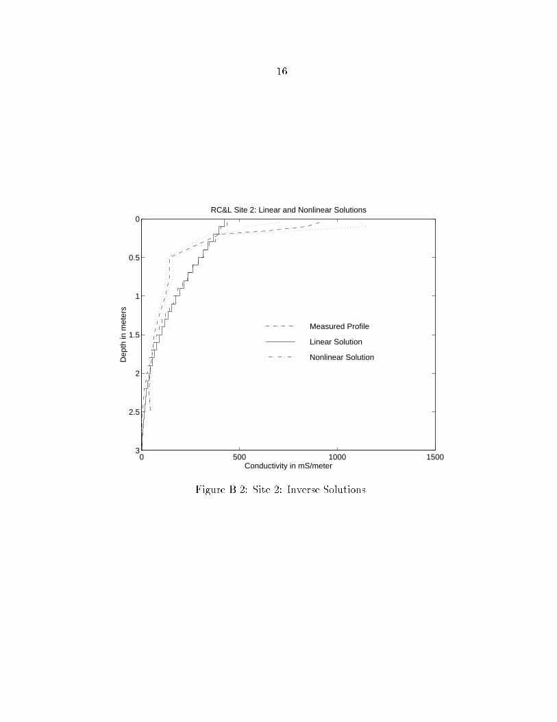
B�� Site �� Inverse Solutions� � � � � � � � � � � � � � � � � � � � � � � ��
B�� Site �� Inverse Solutions� � � � � � � � � � � � � � � � � � � � � � � ��
B�� Site �� Inverse Solutions� � � � � � � � � � � � � � � � � � � � � � � ��
B�� Site �� Inverse Solutions� � � � � � � � � � � � � � � � � � � � � � � ��
B�� Site �� Inverse Solutions� � � � � � � � � � � � � � � � � � � � � � � ��
B�� Site �� Inverse Solutions� � � � � � � � � � � � � � � � � � � � � � � ��
B�� Site �� Inverse Solutions� � � � � � � � � � � � � � � � � � � � � � � ��
B�� Site �� Inverse Solutions� � � � � � � � � � � � � � � � � � � � � � � ��
B��� Site ��� Inverse Solutions� � � � � � � � � � � � � � � � � � � � � � ��
B��� Site ��� Inverse Solutions� � � � � � � � � � � � � � � � � � � � � � ��
B��� Site ��� Inverse Solutions� � � � � � � � � � � � � � � � � � � � � � ��
B��� Site ��� Inverse Solutions� � � � � � � � � � � � � � � � � � � � � � ��
B��� Site ��� Inverse Solutions� � � � � � � � � � � � � � � � � � � � � � ��
C�� Site �� Linear Lcurve� � � � � � � � � � � � � � � � � � � � � � � � ��
C�� Site �� Linear Lcurve� � � � � � � � � � � � � � � � � � � � � � � � ��
C�� Site �� Linear Lcurve� � � � � � � � � � � � � � � � � � � � � � � � ��
C�� Site �� Linear Lcurve� � � � � � � � � � � � � � � � � � � � � � � � ��
C�� Site �� Linear Lcurve� � � � � � � � � � � � � � � � � � � � � � � � ��
C�� Site �� Linear Lcurve� � � � � � � � � � � � � � � � � � � � � � � � ��
ix
C�� Site �� Linear Lcurve� � � � � � � � � � � � � � � � � � � � � � � � ��
C�� Site �� Linear Lcurve� � � � � � � � � � � � � � � � � � � � � � � � ��
C�� Site �� Linear Lcurve� � � � � � � � � � � � � � � � � � � � � � � � ��
C��� Site ��� Linear Lcurve� � � � � � � � � � � � � � � � � � � � � � � ��
C��� Site ��� Linear Lcurve� � � � � � � � � � � � � � � � � � � � � � � ��
C��� Site ��� Linear Lcurve� � � � � � � � � � � � � � � � � � � � � � � ��
C��� Site ��� Linear Lcurve� � � � � � � � � � � � � � � � � � � � � � � ��
C��� Site ��� Linear Lcurve� � � � � � � � � � � � � � � � � � � � � � � ��
D�� Site �� Nonlinear Lcurve� � � � � � � � � � � � � � � � � � � � � � ��
D�� Site �� Nonlinear Lcurve� � � � � � � � � � � � � � � � � � � � � � ��
D�� Site �� Nonlinear Lcurve� � � � � � � � � � � � � � � � � � � � � � ��
D�� Site �� Nonlinear Lcurve� � � � � � � � � � � � � � � � � � � � � � ��
D�� Site �� Nonlinear Lcurve� � � � � � � � � � � � � � � � � � � � � � ��
D�� Site �� Nonlinear Lcurve� � � � � � � � � � � � � � � � � � � � � � ��
D�� Site �� Nonlinear Lcurve� � � � � � � � � � � � � � � � � � � � � � ��
D�� Site �� Nonlinear Lcurve� � � � � � � � � � � � � � � � � � � � � � ��
D�� Site �� Nonlinear Lcurve� � � � � � � � � � � � � � � � � � � � � � ��
D��� Site ��� Nonlinear Lcurve� � � � � � � � � � � � � � � � � � � � � � ��
D��� Site ��� Nonlinear Lcurve� � � � � � � � � � � � � � � � � � � � � � ��
D��� Site ��� Nonlinear Lcurve� � � � � � � � � � � � � � � � � � � � � � ��
x

D��� Site ��� Nonlinear Lcurve� � � � � � � � � � � � � � � � � � � � � � ��
D��� Site ��� Nonlinear Lcurve� � � � � � � � � � � � � � � � � � � � � � ��
xi
Chapter �
Introduction to Ill�Posed Inverse Problems
��� Forward� Inverse� and Identi�cation Problems
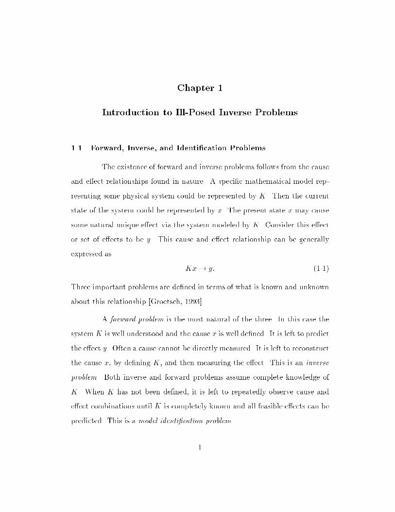
The existence of forward and inverse problems follows from the cause
and eect relationships found in nature� A speci�c mathematical model rep
resenting some physical system could be represented by K� Then the current
state of the system could be represented by x� The present state x may cause
some natural unique eect via the system modeled by K� Consider this eect
or set of eects to be y� This cause and eect relationship can be generally
expressed as
Kx� y� �����
Three important problems are de�ned in terms of what is known and unknown
about this relationship �Groetsch� ������
A forward problem is the most natural of the three� In this case the
systemK is well understood and the cause x is well de�ned� It is left to predict
the eect y� Often a cause cannot be directly measured� It is left to reconstruct
the cause x� by de�ning K� and then measuring the eect� This is an inverse
problem� Both inverse and forward problems assume complete knowledge of
K� When K has not been de�ned� it is left to repeatedly observe cause and
eect combinations until K is completely known and all feasible eects can be
predicted� This is a model identi�cation problem�
�
�
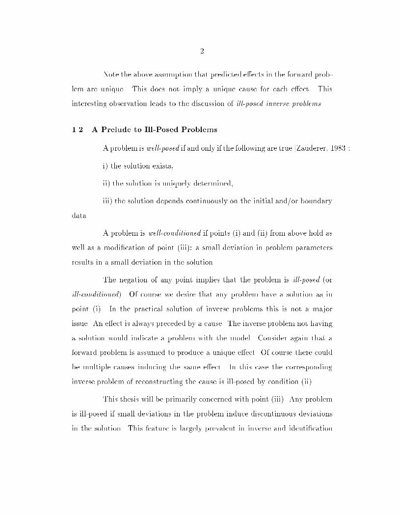
Note the above assumption that predicted eects in the forward prob
lem are unique� This does not imply a unique cause for each eect� This
interesting observation leads to the discussion of ill�posed inverse problems�
��� A Prelude to Ill�Posed Problems
A problem is well�posed if and only if the following are true �Zauderer� ������
i� the solution exists�
ii� the solution is uniquely determined�
iii� the solution depends continuously on the initial and�or boundary
data�
A problem is well�conditioned if points �i� and �ii� from above hold as
well as a modi�cation of point �iii�� a small deviation in problem parameters
results in a small deviation in the solution�
The negation of any point implies that the problem is ill�posed �or
ill�conditioned�� Of course we desire that any problem have a solution as in
point �i�� In the practical solution of inverse problems this is not a major
issue� An eect is always preceded by a cause� The inverse problem not having
a solution would indicate a problem with the model� Consider again that a
forward problem is assumed to produce a unique eect� Of course there could
be multiple causes inducing the same eect� In this case the corresponding
inverse problem of reconstructing the cause is illposed by condition �ii��
This thesis will be primarily concerned with point �iii�� Any problem
is illposed if small deviations in the problem induce discontinuous deviations
in the solution� This feature is largely prevalent in inverse and identi�cation
�
problems� In fact� illposedness in this sense is extremely problematic� any
measurement error is essentially a small parameter deviation� The implications
will be discussed at the end of chapter �� We proceed by examining three
problems that are either illposed or illconditioned�
��� Ill�Posed Inverse Problems
These examples are closely related to the inversion problem stated
in chapter � and solved in the remainder of the thesis� The �rst has simple
intuitive appeal� The last two demonstrate illconditioning and illposedness
in linear algebra and calculus�
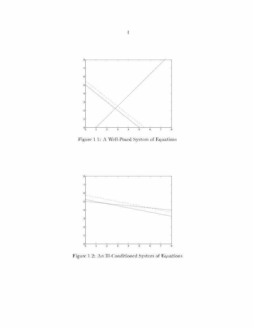
����� A Graphical Example
Consider two lines in a plane� Assume at �rst� that they are nearly
perpendicular and not vertical� Also note that four numbers de�ne the system�
two slopes and two yintercepts� For this system the solution is the point �x� y�
satisfying the equations of both lines� Finally we consider a tiny alteration in
the system� Allow a small deviation in either of the yintercepts� This small
change results in a correspondingly small change in the solution as shown in
�gure ����
Now again consider two lines in a plane but assume they are nearly
parallel� The solution of this system of equations is still the intersection� But
a small deviation in either yintercept results in a remarkably large change in
the solution� This is demonstrated in �gure ����
In the �rst case the solution was insensitive to small system devia
�
0 1 2 3 4 5 6 7 80
1
2
3
4
5
6
7
8
Figure ���� A WellPosed System of Equations�
0 1 2 3 4 5 6 7 80
1
2
3
4
5
6
7
8
Figure ���� An IllConditioned System of Equations�
�
tions� In the second case the solution to the system of equations is very sensitive
to changes in the intercept� This system is ill�conditioned�
����� A Linear Algebra Example
We will look now at an adaptation of an example by Hansen �Hansen� ������
Consider the system of equations Ax � b�� where
A �
�B� ���� ����
���� �������� ����
�CA � and b� �
�B� ����
��������
�CA �����
There exists an exact solution x� �
���
�� As in ����� we consider
the eect of a small perturbation of b��
Let b� �
�B�
���� �������� �������� ����
�CA�
��
��
�B�
�������������
�CA �
�B�
������������
�CA �����
This results in the over determined system of equations Ax� � b��
Though there is no exact solution� it is natural to seek a least squares solution�
that is� to �nd
minxkAx� b�k�where k � k� is the Euclidean �norm� This solution is xLSQ �
����������
�� A
relatively small change in a system parameter� b�� induced a huge change in
the solution x�
Recall that if we take A to be acting on x to yield a measurable result
b� then �nding x for a given b is an ill�conditioned inverse problem� Section
��� demonstrates how an illposed inverse problem can be discretized into an
illconditioned inverse problem�
�
����� Systems of Linear Equations and Condition Numbers
As shown by Forsythe �Forsythe et al�� ������ one can conveniently
de�ne the condition number of a matrix so as to develop a relationship be
tween the relative change in b and the relative error in the solution for x� The
de�nition can be based on the �� �� or � norms� denoted k � k�� k � k�� or k � k�respectively�
Given a square matrix A and a nonzero vector x� let bx � Ax� The
condition number of A is de�ned as
cond�A� �M
m� where �����
M � maxxkAxkkxk � maxx
kbxkkxk �����
and m � minxkAxkkxk � minx
kbxkkxk �����
By de�nition� M is equivalent to the conditional matrix norm of A with respect
to the given vector norm and is denoted by� M � kAk� This can be used to
�nd an alternate de�nition of cond�A� for nonsingular square matrices� Starting
with the de�nition of m� we have
m � minxkAxkkxk �����
� minxkAA��xkkA��xk �����
� minxkxk
kA��xk �����
�
��
maxxkA��xkkxk
������
��
kA��k ������
Taking cond�A� to be the ratio of M to m� we are left with
cond�A� �M
m� kAk �
�kA��k
� kAkkA��k ������
This approach only works if A is both nonsingular and square�
Now if b is perturbed by an amount �b� then the inverse solution
of Ax � b is perturbed by an amount �x� Then we have the new system of
equations
A�x��x� � b��b� ������
It follows that A��x� � �b� By the de�nitions of m and M we have both
mk�xk � k�bk ������
and Mkxk � kbk ������
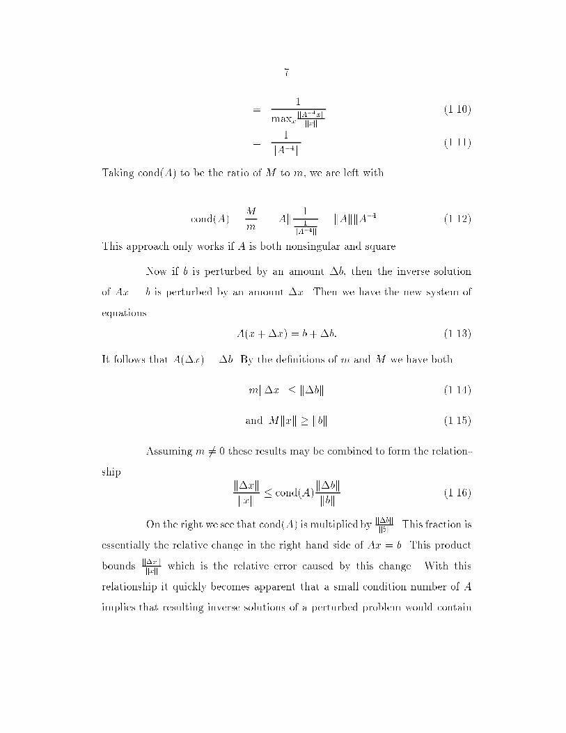
Assuming m �� � these results may be combined to form the relation
shipk�xkkxk � cond�A�
k�bkkbk ������
On the right we see that cond�A� is multiplied by k�bkkbk � This fraction is
essentially the relative change in the right hand side of Ax � b� This product
bounds k�xkkxk which is the relative error caused by this change� With this
relationship it quickly becomes apparent that a small condition number of A
implies that resulting inverse solutions of a perturbed problem would contain
�
little error� A large condition number provides a large upper bound on the
relative error� Such a system is said to be an ill�conditioned system of equations�
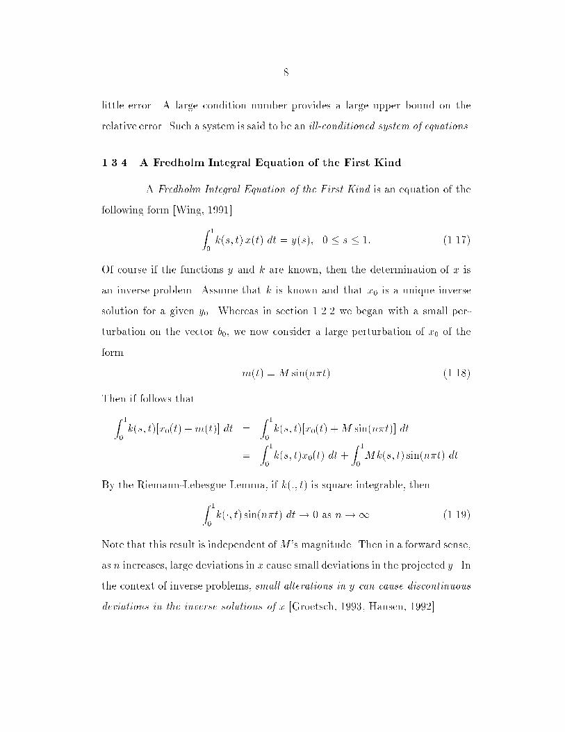
���� A Fredholm Integral Equation of the First Kind
A Fredholm Integral Equation of the First Kind is an equation of the
following form �Wing� �����
Z �
�k�s� t�x�t� dt � y�s�� � � s � �� ������
Of course if the functions y and k are known� then the determination of x is
an inverse problem� Assume that k is known and that x� is a unique inverse
solution for a given y�� Whereas in section ����� we began with a small per
turbation on the vector b�� we now consider a large perturbation of x� of the
form
m�t� � M sin�n�t� ������
Then if follows that
Z �
�k�s� t��x��t� �m�t�� dt �
Z �
�k�s� t��x��t� �M sin�n�t�� dt
�Z �
�k�s� t�x��t� dt�
Z �
�Mk�s� t� sin�n�t� dt
By the RiemannLebesgue Lemma� if k��� t� is square integrable� then
Z �
�k��� t� sin�n�t� dt� � as n�� ������
Note that this result is independent ofM �s magnitude� Then in a forward sense�
as n increases� large deviations in x cause small deviations in the projected y� In
the context of inverse problems� small alterations in y can cause discontinuous
deviations in the inverse solutions of x �Groetsch� ����� Hansen� ������
�
Many problems in the physical sciences� from tomography to geo
magnetic prospecting� can be expressed as Fredholm integral equations of the
�rst kind �Parker� ����� Twomey� ����� Wing� ������ The illposedness of these
equations is particularly problematic to those interested in solving problems in
these �elds�
�� Why Solving These Problems is Important
An understanding of illposed problems is of practical importance to
all those doing mathematical work in the physical sciences� Recall from the
opening discussion that a problem has three parts� a system model� K� a cause
or system state� x� and an eect� y� Most scienti�c problems are either inverse
problems or model identi�cation problems� In the inverse problem the eect
is somehow measured and the cause� of actual interest� is induced� There is
always some sort of error involved in the measurement of y� We would like
the corresponding error involved in determining x to be small as well� The
same sorts of things can be said of the model identi�cation problem� Methods
for dealing with this illconditioned behavior� producing a physically realistic
inverse solution for x� are the topic of chapter two�
Chapter �
Discretization and Regularization� Solving the Ill�Posed
Inverse Problem
Section ����� introduced the Fredholm Integral Equation of the First
Kind� Z �
�k�s� t�x�t� dt � y�s�� �����
Section ����� introduced over determined systems of equations� In these cases
illposed and illconditioned behavior was demonstrated� This chapter will
focus on three general methods for solving illconditioned systems of equations�
First� however� we will recall the continuous Fredholm integral equation and
demonstrate its relationship to linear systems of equations�
��� Discretizing the Fredholm Integral Equation of the First Kind
In many physical applications x�t� and y�t� are continuous univariate
functions� To solve the inverse problem� one observes y and deduces x� It is
usually impractical to observe y in a continuous sense� For example t may
represent time and y may represent some time dependent quantity such as
position that is measured at certain points in time� Because y is not completely
known� at best we can only discretely approximate x�
Consider the discretization of the linear Fredholm integral equation
�Groetsch� ����� Wing� ������ We measure y at points s�� s�� ���� sM� This yields
��
��
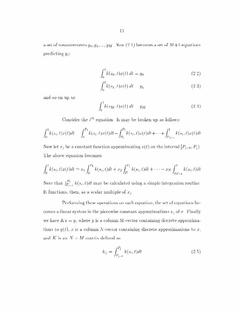
a set of measurements y�� y�� ���� yM� Now ����� becomes a set ofM�� equations
predicting yi�
Z �
�k�s�� t�x�t� dt � y� �����
Z �
�k�s�� t�x�t� dt � y� �����
and so on up to Z �
�k�sM � t�x�t� dt � yM �����
Consider the ith equation� It may be broken up as follows�
Z �
�k�si� t�x�t�dt �
Z P�
�k�si� t�x�t�dt�
Z P�
P�
k�si� t�x�t�dt�����Z �
PN��
k�si� t�x�t�dt
Now let xj be a constant function approximating x�t� on the interval �Pj��� Pj��
The above equation becomes
Z �
�k�si� t�x�t�dt � x�
Z P�
�k�si� t�dt� x�
Z P�
P�
k�si� t�dt� � � �� xN
Z �
pN��
k�si� t�dt
Note thatR PjPj��
k�si� t�dt may be calculated using a simple integration routine�
It functions� then� as a scalar multiple of xj�
Performing these operations on each equation� the set of equations be
comes a linear system in the piecewise constant approximations xj of x� Finally
we have Kx � y� where y is a column Mvector containing discrete approxima
tions to y�t�� x is a column Nvector containing discrete approximations to x�
and K is an N M matrix de�ned as
kij �Z Pj
Pj��
k�si� t�dt �����
��
�
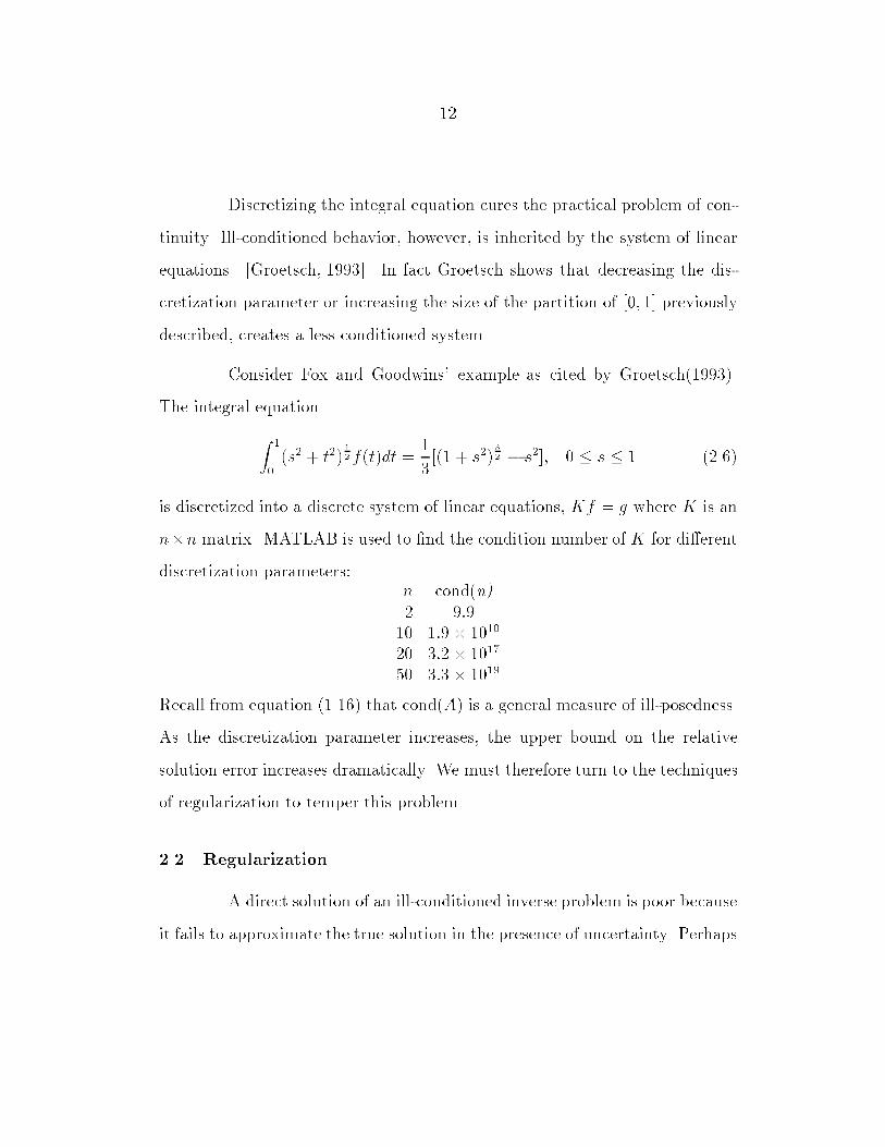
Discretizing the integral equation cures the practical problem of con
tinuity� Illconditioned behavior� however� is inherited by the system of linear
equations �Groetsch� ������ In fact Groetsch shows that decreasing the dis
cretization parameter or increasing the size of the partition of ��� �� previously
described� creates a less conditioned system�
Consider Fox and Goodwins� example as cited by Groetsch�������
The integral equation
Z �
��s� � t��
�
�f�t�dt ��
���� � s��
�
� � s��� � � s � � �����
is discretized into a discrete system of linear equations� Kf � g where K is an
nn matrix� MATLAB is used to �nd the condition number of K for dierent
discretization parameters�n cond�n�� ���
�� ��� ����
�� ��� ����
�� ��� ����
Recall from equation ������ that cond�A� is a general measure of illposedness�
As the discretization parameter increases� the upper bound on the relative
solution error increases dramatically� We must therefore turn to the techniques
of regularization to temper this problem�
��� Regularization
A direct solution of an illconditioned inverse problem is poor because
it fails to approximate the true solution in the presence of uncertainty� Perhaps
��
where the true solution x is almost at� the inverse solution has a large slope�
Or maybe the true solution has little curvature but the inverse solution has a
sharp curvature�
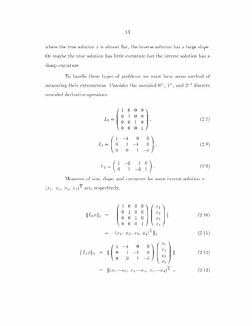
To handle these types of problems we must have some method of
measuring their extremeness� Consider the unscaled �th� �st� and �nd discrete
unscaled derivative operators�
L� �
�BBB�
� � � �� � � �� � � �� � � �
�CCCA � �����
L� �
�B� � �� � �
� � �� �� � � ��
�CA � �����
L� �
�� �� � �� � �� �
�� �����
Measures of size� slope� and curvature for some inverse solution x �
�x�� x�� x�� x�T are� respectively�
kL�xk� � k
�BBB�
� � � �� � � �� � � �� � � �
�CCCA�BBB�
x�x�x�x
�CCCA k ������
� k�x�� x�� x�� x�Tk� ������
kL�xk� � k�B�
� �� � �� � �� �� � � ��
�CA�BBB�
x�x�x�x
�CCCA k ������
� k�x� � x�� x� � x�� x� � x�Tk� ������
��
0 0.5 1 1.5 2 2.5 30
0.5
1
1.5
2
2.5
3Evaluations of x at discrete points of t
ti
x( t i
)
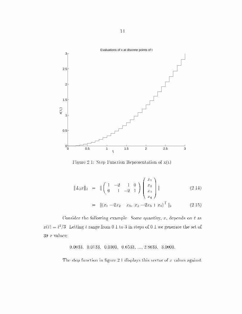
Figure ���� Step Function Representation of x�t��
kL�xk� � k�
� �� � �� � �� �
��BBB�x�x�x�x
�CCCA k ������
� k�x� � �x� � x�� x� � �x� � x�Tk� ������
Consider the following example� Some quantity� x� depends on t as
x�t� � t���� Letting t range from ��� to � in steps of ��� we generate the set of
�� x values�
������� ������� ������� ������� ���� ������� �������
The step function in �gure ��� displays this vector of x values against
��
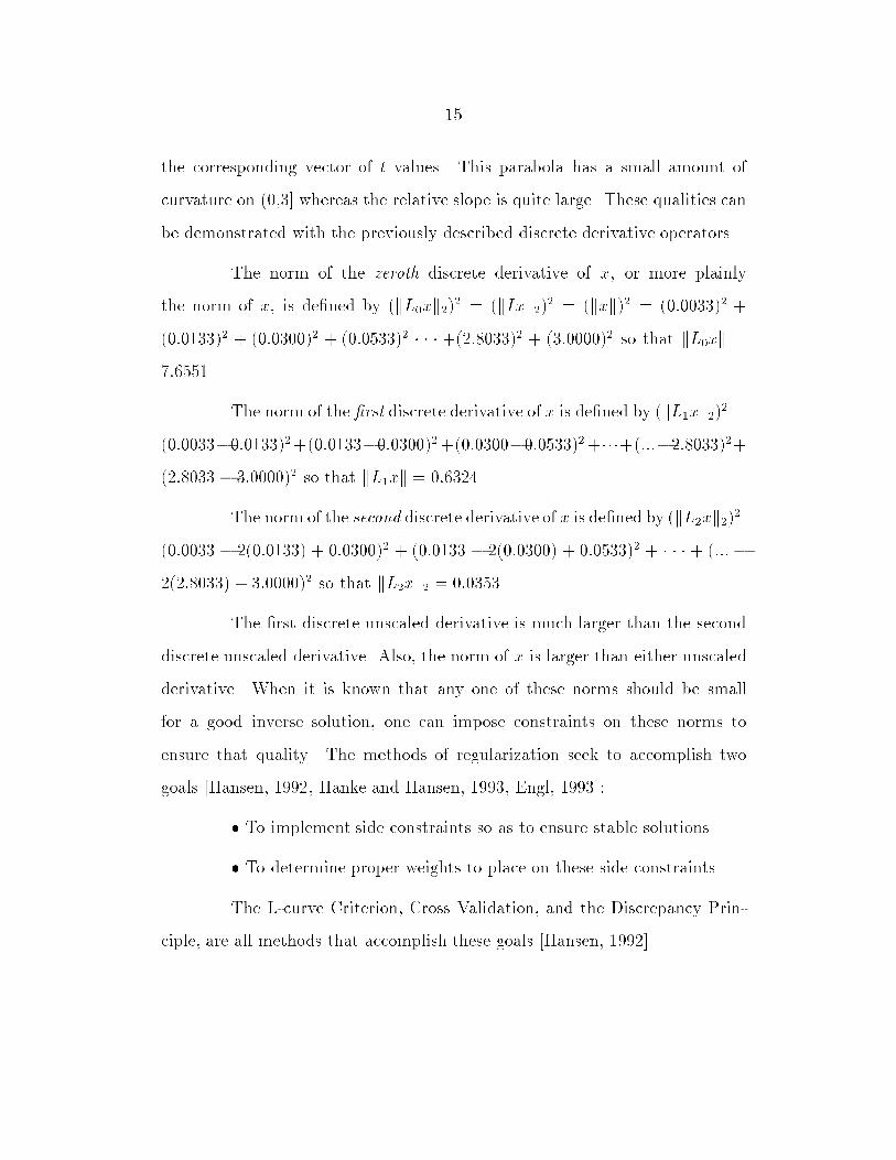
the corresponding vector of t values� This parabola has a small amount of
curvature on ����� whereas the relative slope is quite large� These qualities can
be demonstrated with the previously described discrete derivative operators�
The norm of the zeroth discrete derivative of x� or more plainly
the norm of x� is de�ned by �kL�xk��� � �kIxk��� � �kxk�� � ��������� �
��������� � ��������� � ��������� � � � ���������� � ��������� so that kL�xk �
�������
The norm of the �rst discrete derivative of x is de�ned by �kL�xk��� ����������������������������������������������������������������������
������� � �������� so that kL�xk � �������
The norm of the second discrete derivative of x is de�ned by �kL�xk��� �������� � ��������� � �������� � ������� � ��������� � �������� � � � � � �������������� � �������� so that kL�xk� � �������
The �rst discrete unscaled derivative is much larger than the second
discrete unscaled derivative� Also� the norm of x is larger than either unscaled
derivative� When it is known that any one of these norms should be small
for a good inverse solution� one can impose constraints on these norms to
ensure that quality� The methods of regularization seek to accomplish two
goals �Hansen� ����� Hanke and Hansen� ����� Engl� ������
To implement side constraints so as to ensure stable solutions�
To determine proper weights to place on these side constraints�
The Lcurve Criterion� Cross Validation� and the Discrepancy Prin
ciple� are all methods that accomplish these goals �Hansen� ������
��
����� L�curve Principle
Because a linear Fredholm integral equation may be discretized� we
have at present the general problem
minxkAx� bk�� ������
where x and b are column vectors and A is a matrix�
To smooth out the illconditioned tendencies we append a penalty
function� referred to as the regularization term� involving a discrete derivative
operator �Hansen� ������
minxf kAx� bk�� � ��kLixk�� g� ������
The choice of derivative operator is important� Solutions could be
sensitive to this choice� Of course this requires some assumption on the solution
shape� In the presence of no information one might try several derivative
operators and compare resulting solutions�
A more di�cult subproblem is choosing ��� the weight placed on the
regularization term� Note that any good inverse solution� x�� will impose a
small residual error kAx� � bk�� and a small regularization term kLix�k���
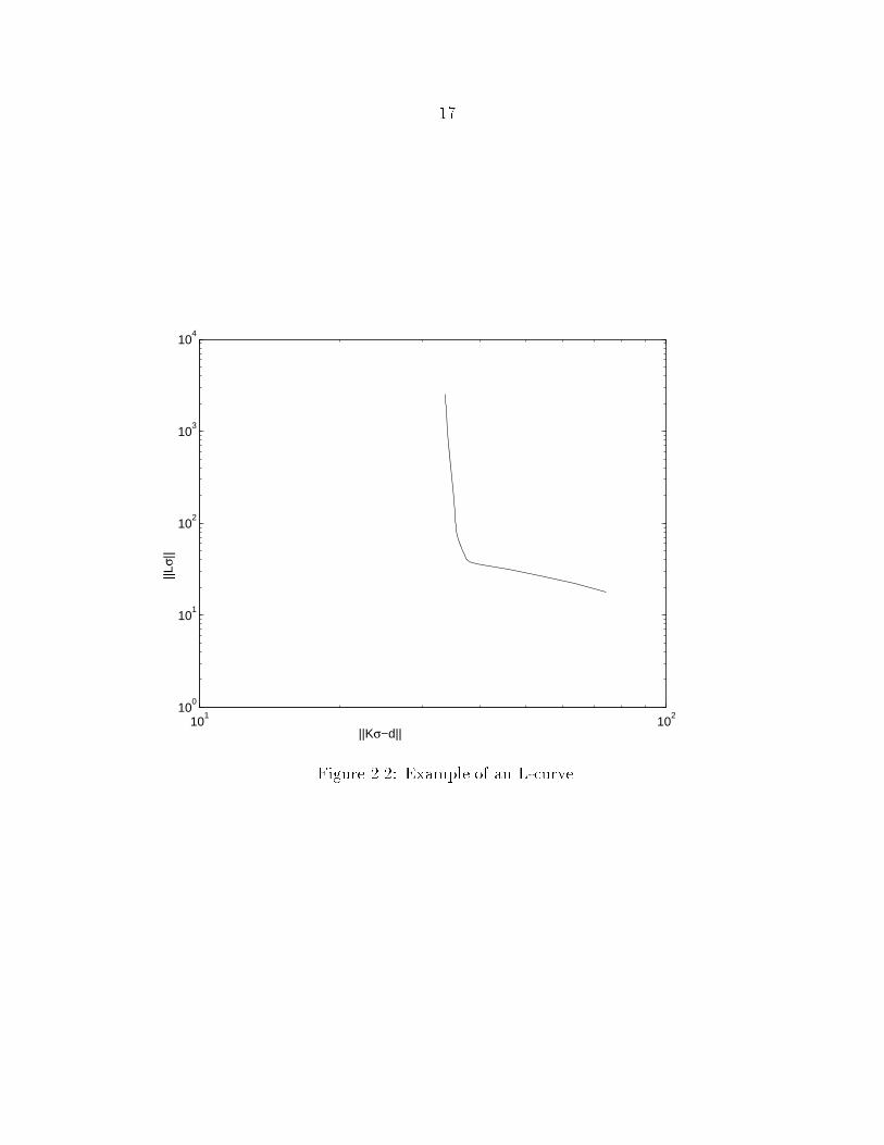
The Lcurve principle is as follows �Hansen� ������ Repeatedly solve
the modi�ed minimization problem with several values of ��� Then for each
value of ��� plot the regularization term against the residual term for the cor
responding inverse solution� x��� In other words plot the set of points
�kAx� � bk� kLix�k�� ������
��
101
102
100
101
102
103
104
||Kσ−d||
||Lσ|
|
Figure ���� Example of an Lcurve�
��
This process will trace out an �Lcurve� as in �gure ����
In practice this curve tends to be an �L� with a de�nite corner� As
�� increases� ow moves down the curve� This is because a large value of ��
is associated with a large weight on the regularization term kLixk��� Then to
properly minimize kAx� bk�� � ��kLixk��� x must be such that kLixk�� is very
small� The residual term kAx� bk�� is allowed to grow� Such a point tends to
be far from the yaxis and close to the xaxis�
The best choice of �� will produce a solution corresponding to the
Lcurve corner� To see why it is best� one can view the corner of �gure�����
and imagine a small improvement being made on either term� If one wants
a solution that is slightly more smooth than the corner solution� then a large
sacri�ce in sum squared error must be made� If one wants a slightly smaller
sum squared error� then a large sacri�ce must be made in smoothness�
The Lcurve criterion can� however� fail to produce a distinct corner�
In this case one may turn to cross validation or the discrepancy principle�
����� Cross�Validation
As with the Lcurve criterion� ordinary cross validation �OCV� is a
method of choosing a good value of �� with respect to ������
minxkAx� bk�� � ��kLixk���
But for notational convenience this section will discuss the identical problem�
minxMXi�
�aix� bi�� � ��
MXi�
�li�p�x��� ������
��
Here ai is the ith row of A and li�p� is the ith row of the pth discrete derivative
operator Lp� In other words� li�p�x is the ith element of Lpx� Again kAx� bk��measures the amount of solution error and Lix is a quality desired to be small�
OCV uses the idea that if some element of b� say bi� is eliminated
from b then a good value of �� will still yield a good solution �Hansen� �����
Wahba� ������ It will be good in that the resulting solution x�� will predict a
vector b� that can be used to interpolate the missing element� bi� Of course the
mis�t of this prediction is jbi � b�ij�
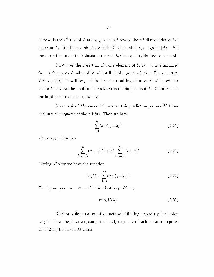
Given a �xed ��� one could perform this prediction process M times
and sum the squares of the mis�ts� Then we have
MXi�
�a�x���i � bi�
� ������
where x���i minimizes
MXj��j �i
�aj � bj�� � ��
MXj��j �i
�lj�p�x�� ������
Letting �� vary we have the function
V ��� �MXI�
�aix���i � bi�
� ������
Finally we pose an �external� minimization problem�
min�V ���� ������
OCV provides an alternative method of �nding a good regularization
weight� It can be� however� computationally expensive� Each instance requires
that ������ be solved M times�
��
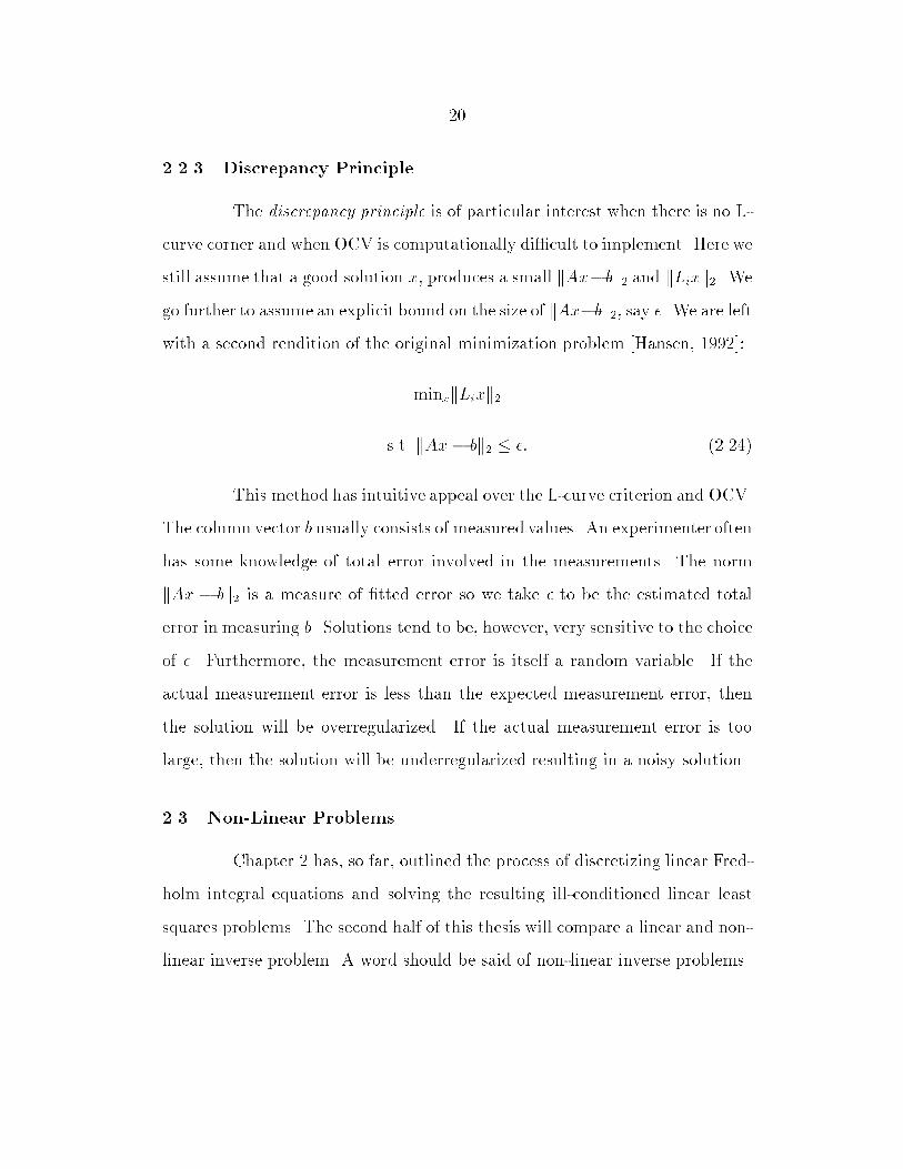
����� Discrepancy Principle
The discrepancy principle is of particular interest when there is no L
curve corner and when OCV is computationally di�cult to implement� Here we
still assume that a good solution x� produces a small kAx�bk� and kLixk�� We
go further to assume an explicit bound on the size of kAx�bk�� say �� We are left
with a second rendition of the original minimization problem �Hansen� ������
minxkLixk�
s�t� kAx� bk� � �� ������
This method has intuitive appeal over the Lcurve criterion and OCV�
The column vector b usually consists of measured values� An experimenter often
has some knowledge of total error involved in the measurements� The norm
kAx � bk� is a measure of �tted error so we take � to be the estimated total
error in measuring b� Solutions tend to be� however� very sensitive to the choice
of �� Furthermore� the measurement error is itself a random variable� If the
actual measurement error is less than the expected measurement error� then
the solution will be overregularized� If the actual measurement error is too
large� then the solution will be underregularized resulting in a noisy solution�
��� Non�Linear Problems
Chapter � has� so far� outlined the process of discretizing linear Fred
holm integral equations and solving the resulting illconditioned linear least
squares problems� The second half of this thesis will compare a linear and non
linear inverse problem� A word should be said of nonlinear inverse problems�
��
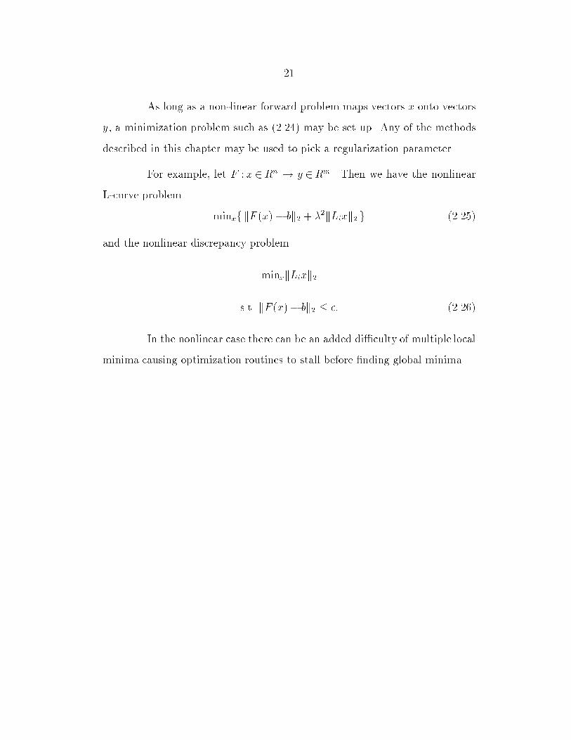
As long as a nonlinear forward problem maps vectors x onto vectors
y� a minimization problem such as ������ may be set up� Any of the methods
described in this chapter may be used to pick a regularization parameter�
For example� let F � x �Rn � y �Rm� Then we have the nonlinear
Lcurve problem
minxf kF �x�� bk� � ��kLixk� g ������
and the nonlinear discrepancy problem
minxkLixk�
s�t� kF �x�� bk� � �� ������
In the nonlinear case there can be an added di�culty of multiple local
minima causing optimization routines to stall before �nding global minima�
Chapter �
The Geonics EM��� Problem
��� The Inversion Problem De�ned
Having examined the techniques of regularization and the need for
them� chapter � provides the physical background for a soil hydrology problem�
Chapter � concludes with a discussion of two dierent predictive models� In
the remaining chapters we apply the introductory material to this problem and
discuss the results�
A soil�s salinity is� by de�nition� the level of dissolved inorganic so
lutes in the soil� There are many instances in which knowing soil salinity is
important� For example� if irrigated agriculture is to remain sustainable� the
salinity within these soils must remain at a tolerable level �Rhoades� ������
These solutes tend to be conductive� When the electrical conductivity
of soil� referred to as ECa� can be directly measured� salinity can be immedi
ately determined� Invasive measurements are� however� both costly and time
consuming� This brings us to the focus of the second half of the thesis� the
non�invasive inversion of soil conductivity from above ground measurements�
Consider an instrument containing two coils of wire� An alternat
ing current is sent through the transmitting coil� This creates an alternating
magnetic �eld that induces current ow in the underlying soil� These currents
create secondary magnetic �elds� Finally the combination of �elds induces a
��
��
secondary voltage in the receiving coil of the EM��� The instrument would
measure the relative strength of these secondary �elds� �Borchers et al�� �����
Wait� ����� McNeill� ����� McNeill� ������
Geonics Limited markets a device called the EM��� Soil Electrical
Conductivity Meter� This machine will be referred to as the EM��� It is
essentially a hand held bar separating two coils of wire� The coils are �xed
with respect to each other and are exactly � meter apart� The coils can be
positioned either vertically or horizontally� It should be noted that the coil
orientation drastically aects the measurements taken� This study uses both
vertical and horizontal measurements at any given height �Borchers et al�� �����
Rhoades� ������
For future reference� the problem of predicting EM�� measurements
from a vertical electrical conductivity pro�le will be referred to as the forward
EM��� problem� Inverting the pro�le from the EM�� measurements is then
the inverse EM��� problem� The remainder of this chapter will discuss a linear
and nonlinear model for the forward and inverse problems�
��
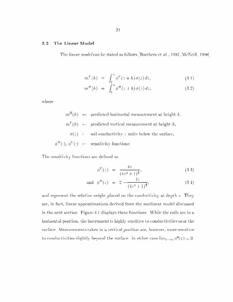
��� The Linear Model
The linear model can be stated as follows �Borchers et al�� ����� McNeill� �����
mV �h� �Z �
��V �z � h��z� dz� �����
mH�h� �Z �
��H�z � h��z� dz� �����
where
mH�h� � predicted horizontal measurement at height h�
mV �h� � predicted vertical measurement at height h�
�z� � soil conductivity z units below the surface�
�H���� �V ��� � sensitivity functions�
The sensitivity functions are de�ned as
�V �z� ��z
��z� � ���
�
� �����
and �H�z� � � � �z
��z� � ���
�
� �����
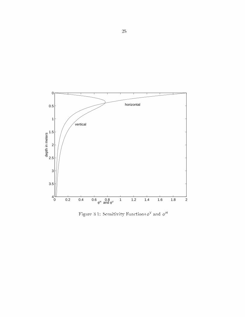
and represent the relative weight placed on the conductivity at depth z� They
are� in fact� linear approximations derived from the nonlinear model discussed
in the next section� Figure ��� displays these functions� While the coils are in a
horizontal position� the instrument is highly sensitive to conductivities near the
surface� Measurements taken in a vertical position are� however� more sensitive
to conductivities slightly beyond the surface� In either case limz�� ���z� � ��
��
0 0.2 0.4 0.6 0.8 1 1.2 1.4 1.6 1.8 2
0
0.5
1
1.5
2
2.5
3
3.5
4
dept
h in
met
ers
φH and φV
horizontal
vertical
Figure ���� Sensitivity Functions�V and �H�
��
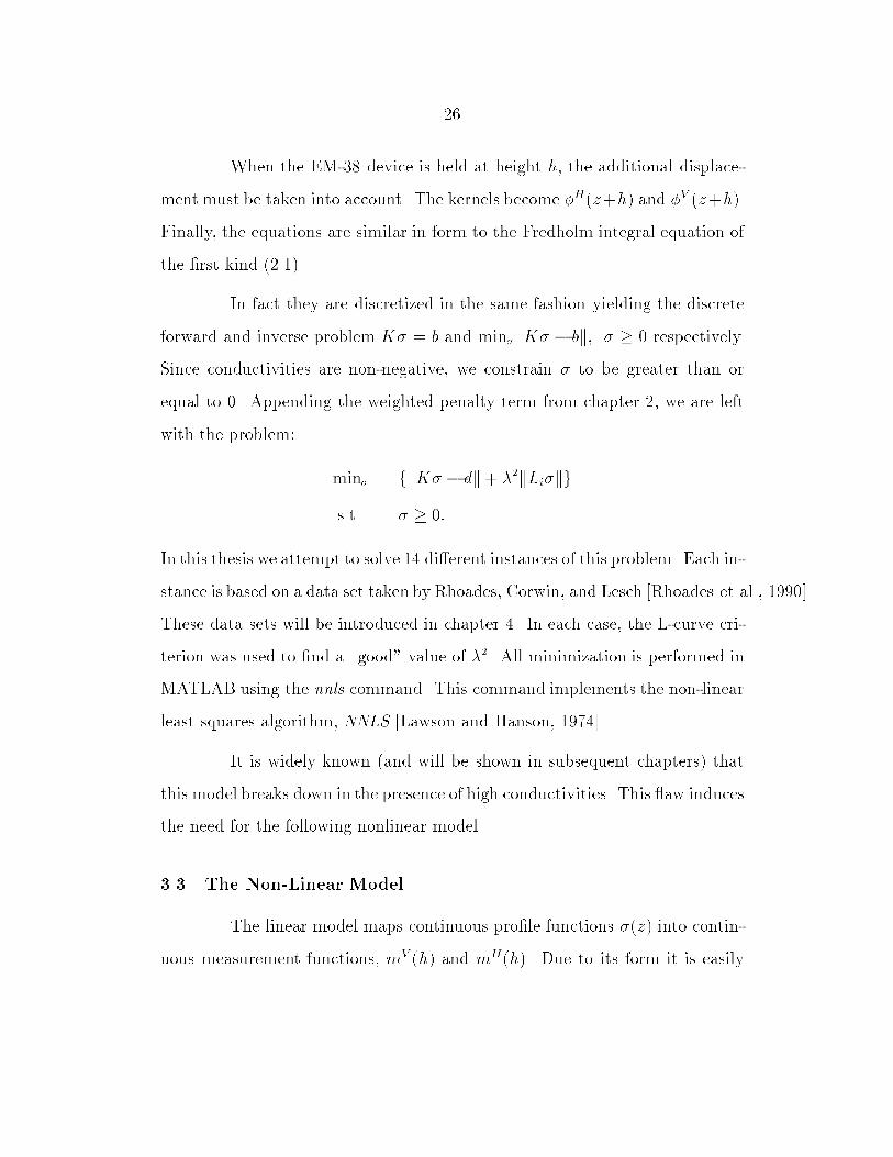
When the EM�� device is held at height h� the additional displace
ment must be taken into account� The kernels become �H�z�h� and �V �z�h��
Finally� the equations are similar in form to the Fredholm integral equation of
the �rst kind ������
In fact they are discretized in the same fashion yielding the discrete
forward and inverse problem K � b and min�kK � bk� � � respectively�
Since conductivities are nonnegative� we constrain to be greater than or
equal to �� Appending the weighted penalty term from chapter �� we are left
with the problem�
min� fkK � dk� ��kLikgs�t� � ��
In this thesis we attempt to solve �� dierent instances of this problem� Each in
stance is based on a data set taken by Rhoades� Corwin� and Lesch �Rhoades et al�� ������
These data sets will be introduced in chapter �� In each case� the Lcurve cri
terion was used to �nd a �good� value of ��� All minimization is performed in
MATLAB using the nnls command� This command implements the nonlinear
least squares algorithm� NNLS �Lawson and Hanson� ������
It is widely known �and will be shown in subsequent chapters� that
this model breaks down in the presence of high conductivities� This aw induces
the need for the following nonlinear model�
��� The Non�Linear Model
The linear model maps continuous pro�le functions �z� into contin
uous measurement functions� mV �h� and mH�h�� Due to its form it is easily
��
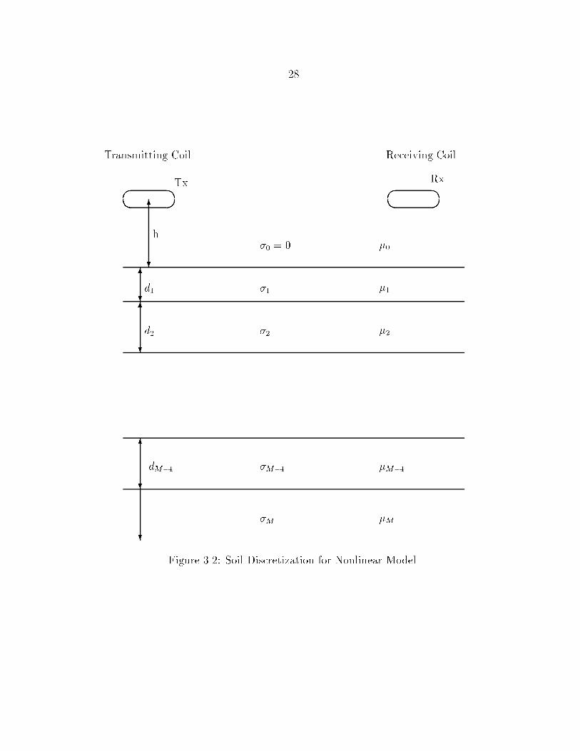
discretized using chapter � techniques� On the other hand� the nonlinear model
must initially assume a discretized soil pro�le� It then maps these conductivity
vectors into a discrete function describing EM�� measurements at dierent
heights� Assume then� that the soil is discretized into M layers where the M th
layer is semiin�nite� Let di represent the thickness of the ith layer and let i
be the conductivity of this layer� This discretization is seen is �gure ������
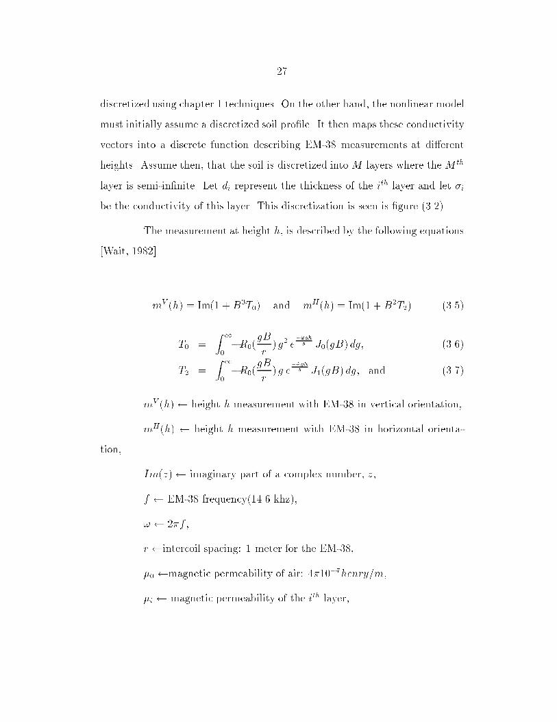
The measurement at height h� is described by the following equations
�Wait� ������
mV �h� � Im�� �B�T�� and mH�h� � Im�� �B�T�� �����
T� �Z �
��R��
gB
r� g� e
��gh
� J��gB� dg� �����
T� �Z �
��R��
gB
r� g e
��gh� J��gB� dg� and �����
mV �h�� height h measurement with EM�� in vertical orientation�
mH�h� � height h measurement with EM�� in horizontal orienta
tion�
Im�z�� imaginary part of a complex number� z�
f � EM�� frequency����� khz��
� ��f �
r�intercoil spacing� � meter for the EM���
�� �magnetic permeability of air� ������henry�m�
�i � magnetic permeability of the ith layer�
��
Transmitting Coil Receiving Coil
��
��
��
��
�
��
�
�
�
�
�
�
Tx Rx
dM��
d�
d� �
�
M��
��
��
�M��
M �M
h� � � ��
Figure ���� Soil Discretization for Nonlinear Model�
��
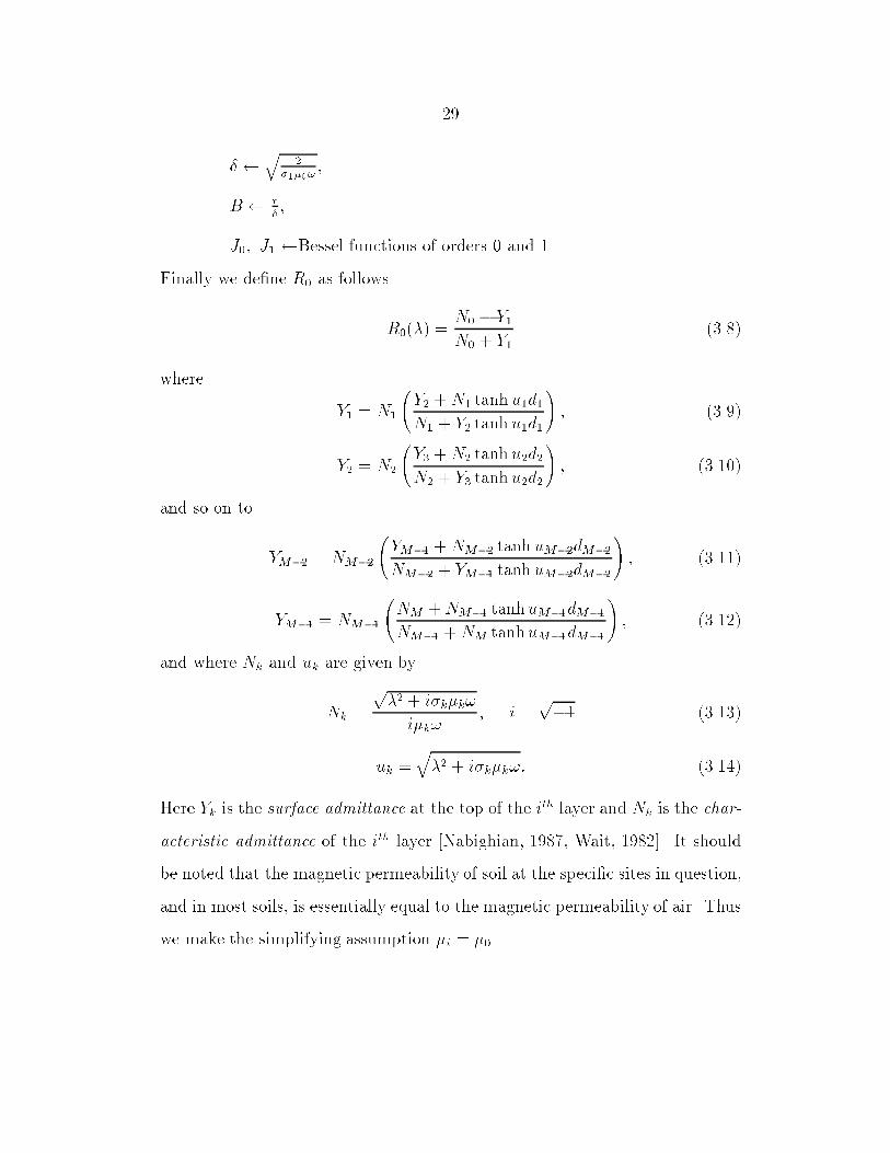
��q
������
�
B � r
��
J�� J� �Bessel functions of orders � and ��
Finally we de�ne R� as follows
R���� �N� � Y�N� � Y�
�����
where
Y� � N�
�Y� �N� tanh u�d�N� � Y� tanh u�d�
�� �����
Y� � N�
�Y� �N� tanh u�d�N� � Y� tanh u�d�
�� ������
and so on to
YM�� � NM��
�YM�� �NM�� tanh uM��dM��
NM�� � YM�� tanh uM��dM��
�� ������
YM�� � NM��
�NM �NM�� tanhuM��dM��
NM�� �NM tanhuM��dM��
�� ������
and where Nk and uk are given by
Nk �
p�� � ik�k
i�k� i �
p�� ������
uk �q�� � ik�k� ������
Here Yk is the surface admittance at the top of the ith layer and Nk is the char�
acteristic admittance of the ith layer �Nabighian� ����� Wait� ������ It should
be noted that the magnetic permeability of soil at the speci�c sites in question�
and in most soils� is essentially equal to the magnetic permeability of air� Thus
we make the simplifying assumption �i � ���
��
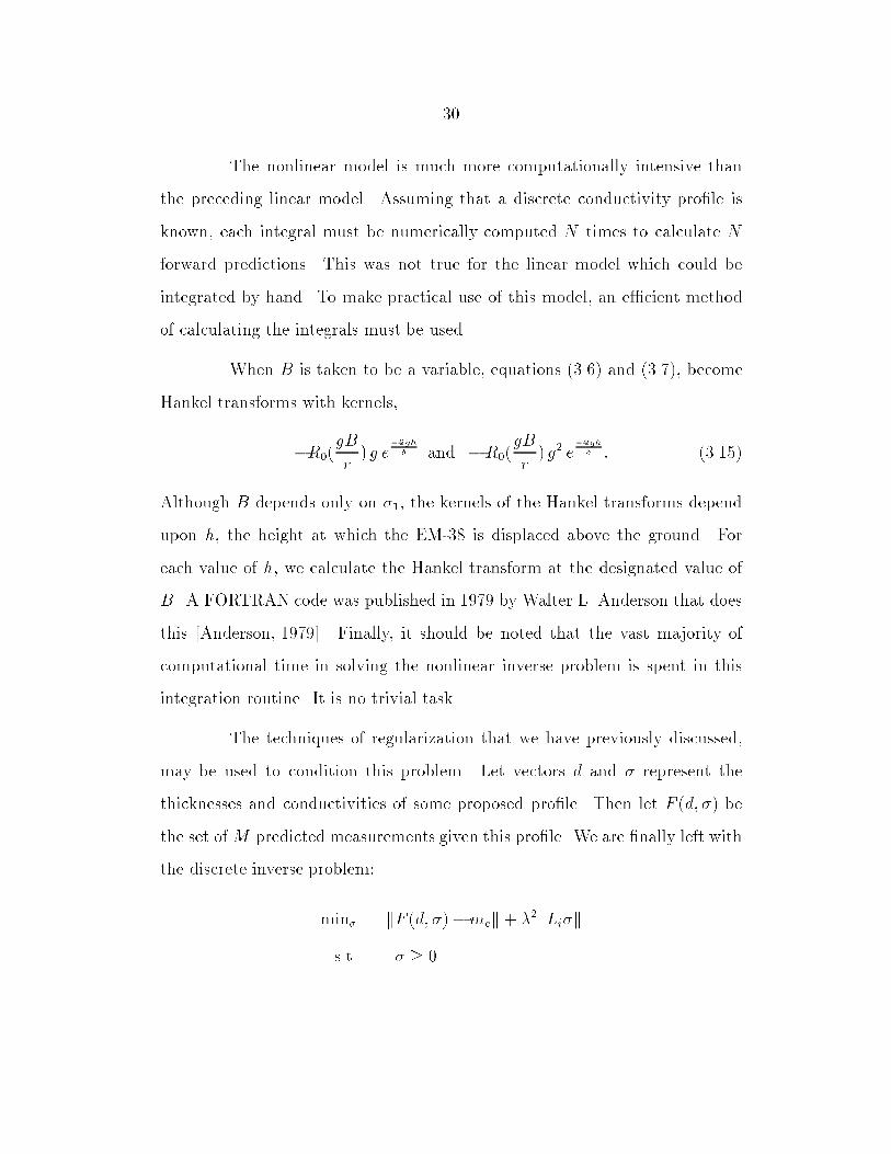
The nonlinear model is much more computationally intensive than
the preceding linear model� Assuming that a discrete conductivity pro�le is
known� each integral must be numerically computed N times to calculate N
forward predictions� This was not true for the linear model which could be
integrated by hand� To make practical use of this model� an e�cient method
of calculating the integrals must be used�
When B is taken to be a variable� equations ����� and ������ become
Hankel transforms with kernels�
�R��gB
r� g e
��gh� and �R��
gB
r� g� e
��gh� � ������
Although B depends only on �� the kernels of the Hankel transforms depend
upon h� the height at which the EM�� is displaced above the ground� For
each value of h� we calculate the Hankel transform at the designated value of
B� A FORTRAN code was published in ���� by Walter L� Anderson that does
this �Anderson� ������ Finally� it should be noted that the vast majority of
computational time in solving the nonlinear inverse problem is spent in this
integration routine� It is no trivial task�
The techniques of regularization that we have previously discussed�
may be used to condition this problem� Let vectors d and represent the
thicknesses and conductivities of some proposed pro�le� Then let F �d� � be
the set of M predicted measurements given this pro�le� We are �nally left with
the discrete inverse problem�
min� kF �d� ��mek� ��kLiks�t� � �
��
where me is an actual set of EM�� measurements�
Whereas MATLAB was a suitable environment to run the linear for
ward and inverse problems� a FORTRAN code had to be constructed to solve
the related nonlinear problems� The nonlinear least squares portion was solved
with a double precision IMSL subroutine called DBCLSF� To guard against the
possibility of �nding a local minimum point a multistart approach was used�
First a set of logarithmically spaced ��s was chosen� For each value
of ��� three initial guesses were chosen� After the three runs were completed
the �best� solution was taken to be the solution with the lowest function value�
Finally an Lcurve was constructed� This study constructed Lcurves by �tting
cubic splines around the points �kK�� datak� kL�k�� Then a new plot was
made for each site of the calculated curvature vs� the value of ��� The highest
point on this curve is the point of greatest curvature or the �Lcurve corner��
ECa readings are known to rarely fall at or above ���� mS�m and
never below � mS�m within the �rst few meters of earth� Occasionally this �L
curve corner� yields a solution that is underregularized in that the maximum
and minimum conductivities are either zero or too large� With this in mind
an additional rule was adopted� if a solution reaches either � or ���� mS�m
before � meters� then �� is increased until a solution within these constraints
is found�
The only detail left to de�ne is the choice of initial guesses for the
multistart method� For the sites discussed in chapter �� the largest ECa reading
is about twice the largest EM�� reading� Thus one initial guess is taken to be
a constant vector of the largest reading and another initial guess is taken to

��
be the twice the largest guess� The third initial guess is taken to be the best
solution from the last set of three runs�
Chapter
Forward Results
Chapters � and � compare the performance of the two preceding mod
els using data sets from �� dierent sites� This data is supplied to us through
a technical report by Rhoades� Corwin� and Lesch �Rhoades et al�� ������ We
will begin chapter � with a discussion of this data� Then this data will be used
to compare forward predictions� In chapter � we will compare inverse solutions�
�� The Rhoades� Corwin� and Lesch Data Sets
A total of �� sites throughout California were chosen� At each site
detailed soil electrical conductivity� ECa� and Geonics EM�� measurements
were taken�
Before actually taking ECa readings� the top soil was leveled o and
dry mulch was removed� Readings were taken at depths of �� ��� ��� ��� ���
��� ���� ���� ���� �������� ���� and ��� cm� At each depth� � readings were
taken� These � readings were spaced on a ��cm��cm grid� Measurements
down to �� cm were taken by vertically inserting a �Martek bedding probe�� A
Martek �Rhoadesprobe� was inserted horizontally for depths ����� cm� To
make this possible a trench was excavated in the EW direction� To sample
the �nal meter� the top � meters were stripped o and a �Rhoadesprobe� was
inserted vertically�
��
��
At each site� EM�� measurements were taken at heights �� ��� ���
��� ��� ��� ��� ���� and ��� cm� At each height� � measurements were taken�
For both horizontal and vertical orientations of the EM��� a measurement was
taken with the instrument facing directions �N� NE� E� SE��
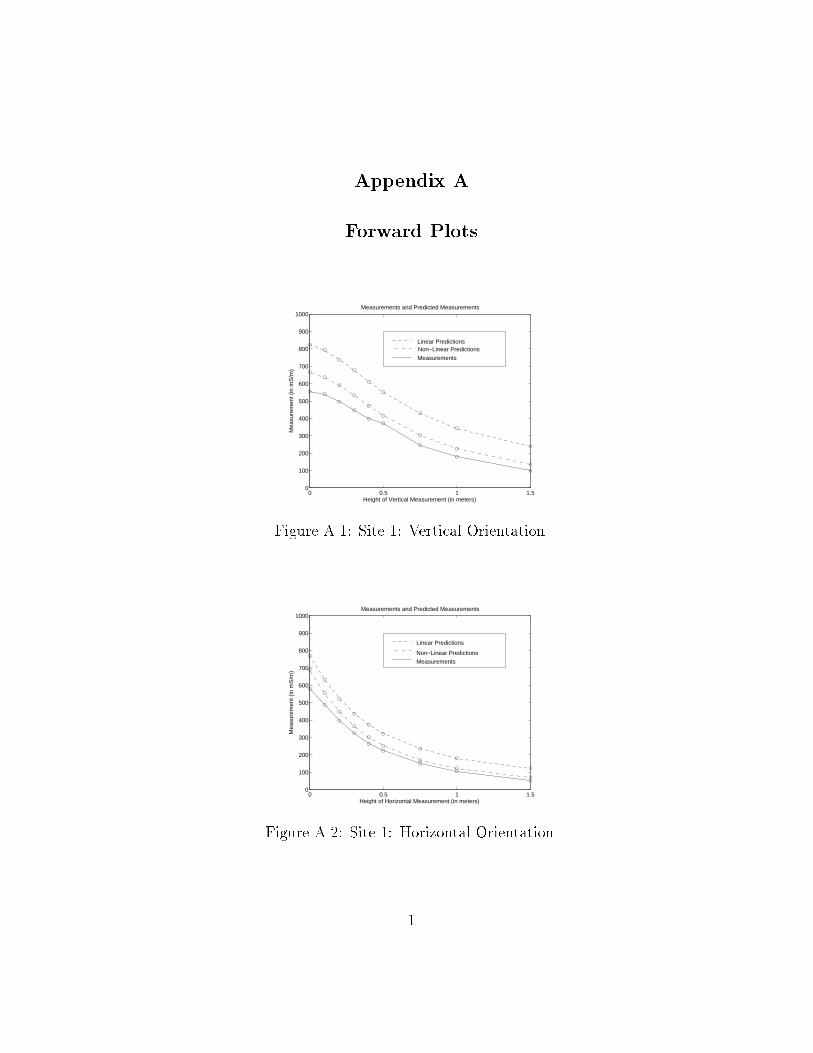
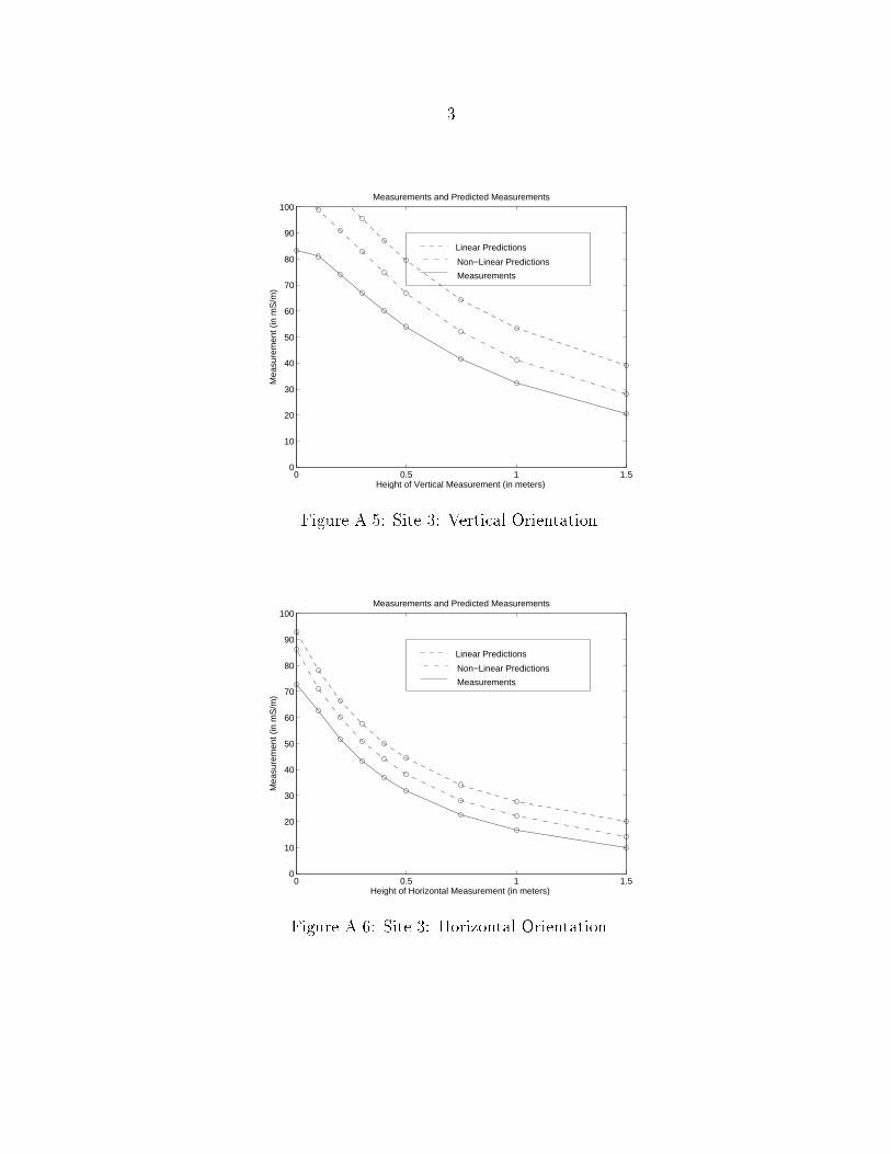
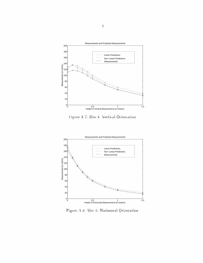
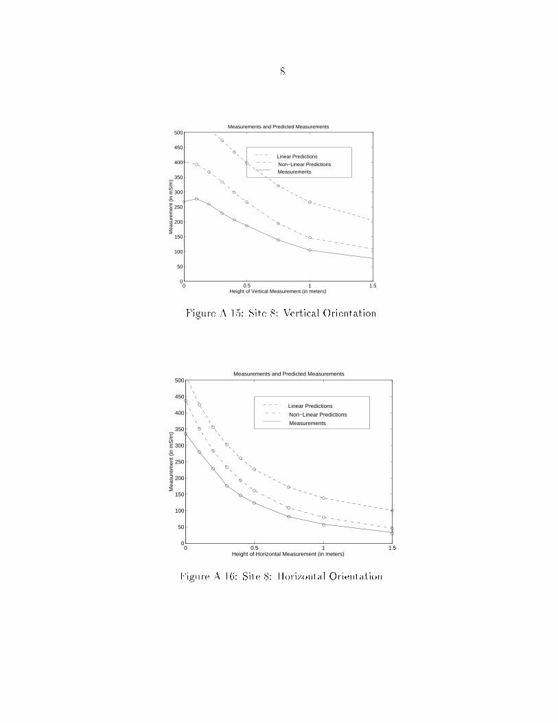
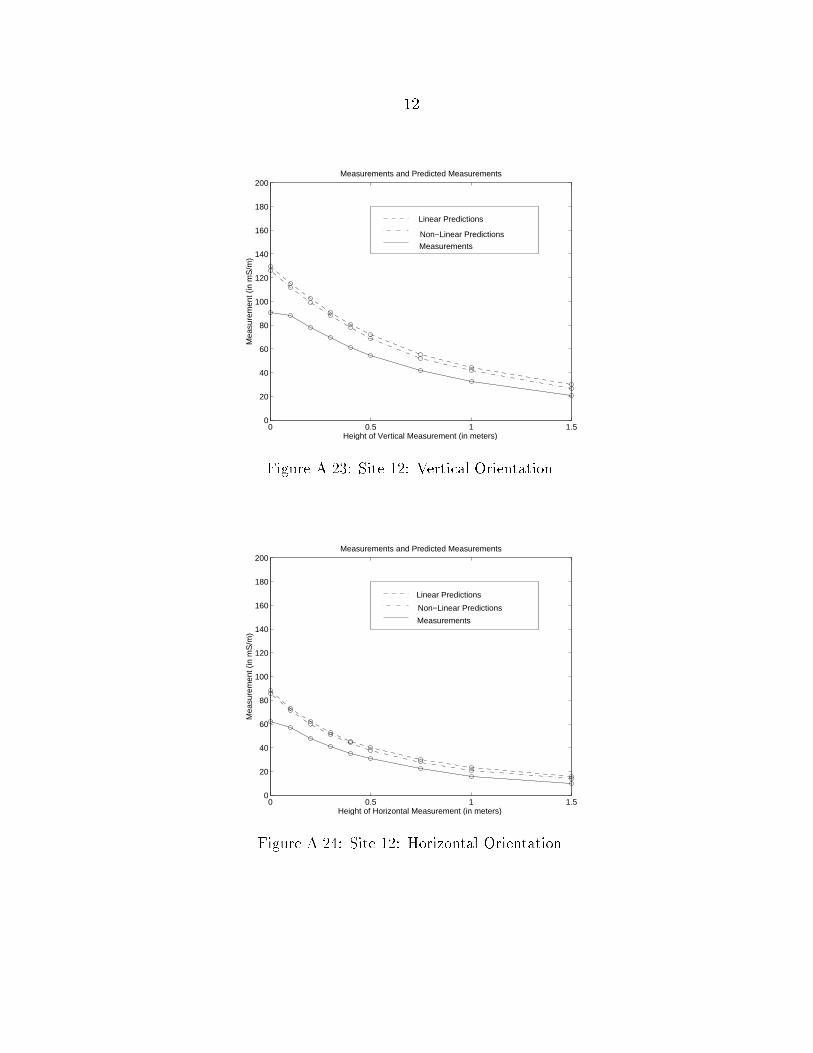
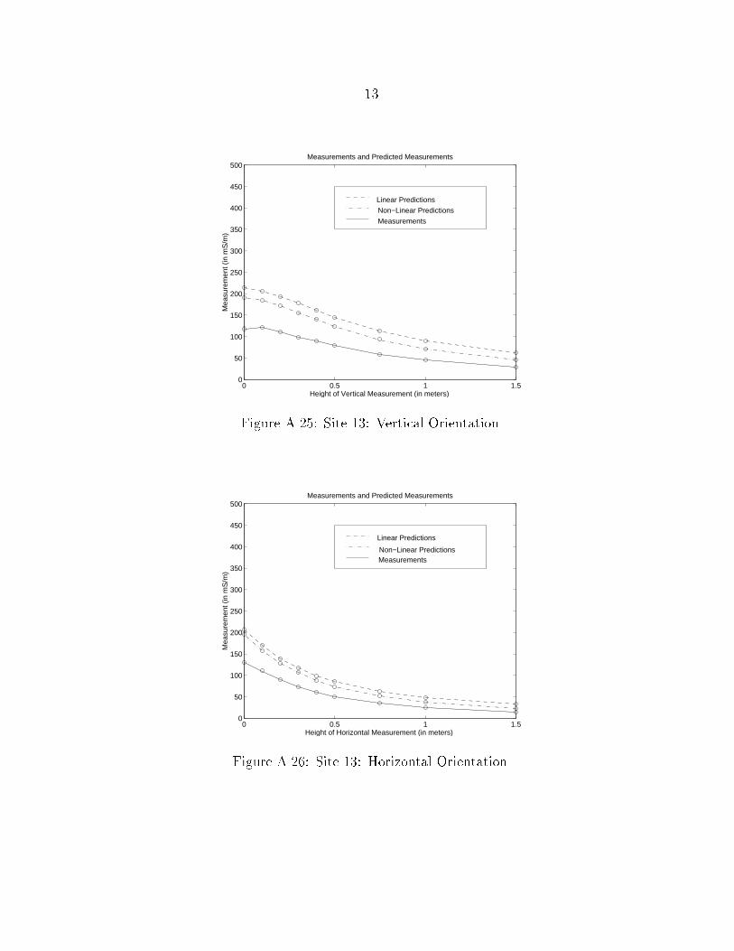
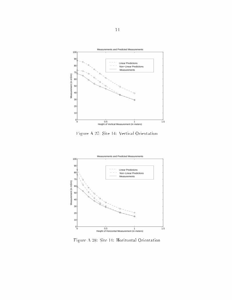
�� Discussion of Forward Plots
The forward plots in appendix A were created in the following manner�
At each depth� the measured soil conductivities were averaged� This pro�le was
then used to interpolate the conductivities of �� cm layers down to � meters
with a semiin�nite layer beginning at the � meter mark� It was assumed that
the conductivity of the semiin�nite layer is the conductivity of the last thin
layer� It was found that the forward predictions are sensitive to this assumption�
More will be said of this later� Finally� using the linear MATLAB code and the
nonlinear FORTRAN code of the previous chapter� forward EM�� predictions
were made at heights �� ��� ��� ��� ��� ��� ��� ���� and ��� cm�
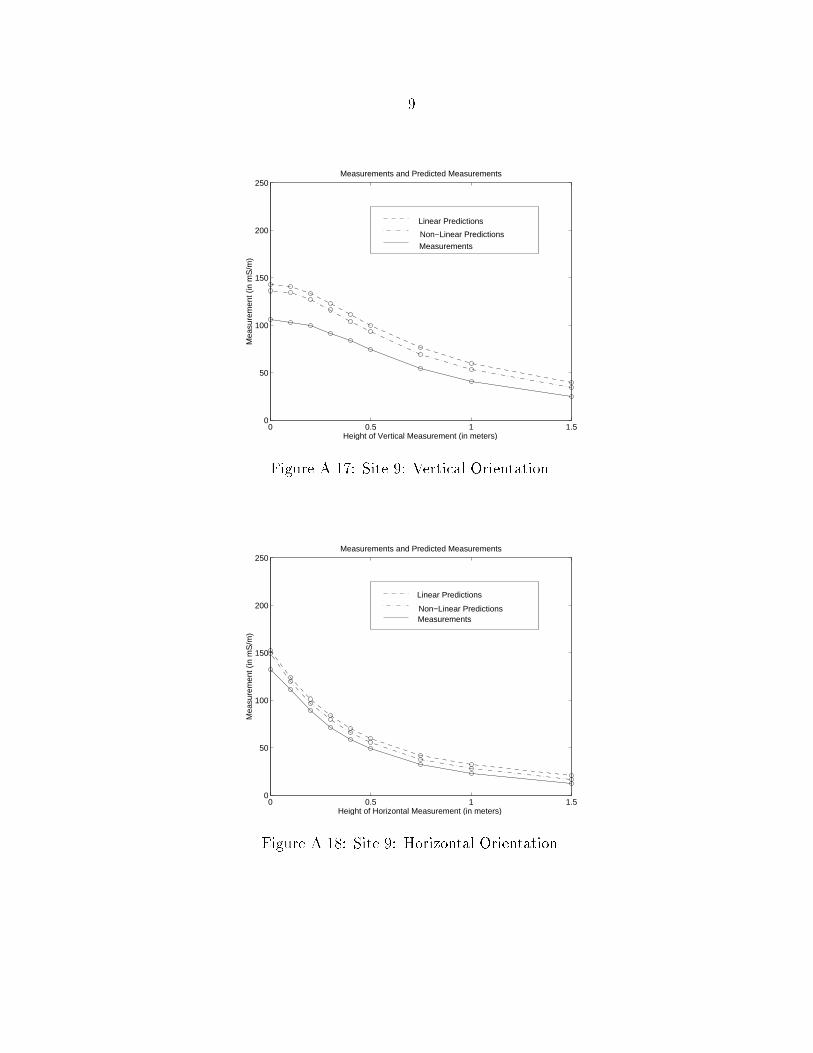
Then for each site� two plots were made� One assuming a vertical
orientation of the instrument and one assuming a horizontal orientation� Each
contains two dotted lines representing predictions of the linear and nonlinear
models� as well as a solid line representing the average EM�� measurement at
each height� There are a total of �� forward plots�
The following observations are a visual interpretation of the �� plots�
Observation Without exception� the nonlinear model outperforms
the linear model� In every plot the nonlinear predictions lie closer to the EM��
measurements than the linear predictions�
��
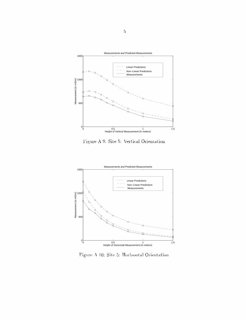
Observation � The linear model always over predicts the EM��� mea�
surements� In fact they are usually over predicted by a substantial amount�
It is not unusual for the linear predictions to be ��� � ���� larger than the
actual measurement�
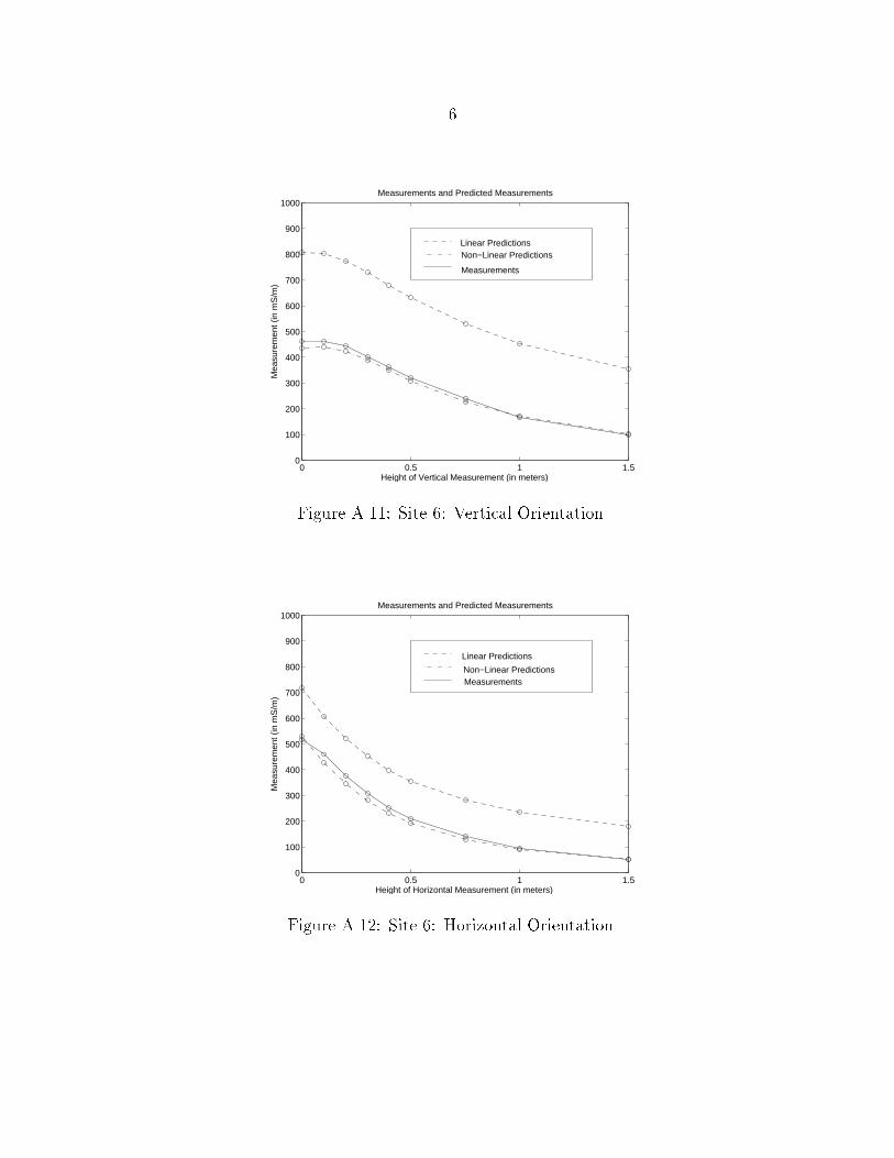
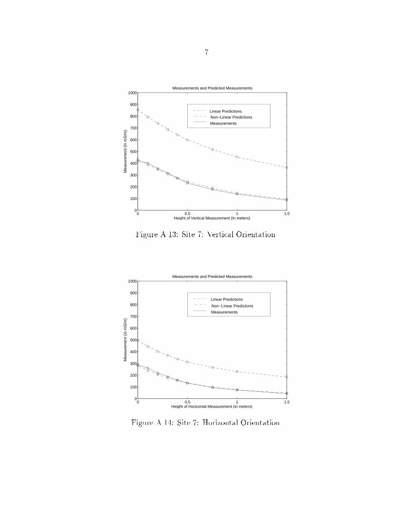
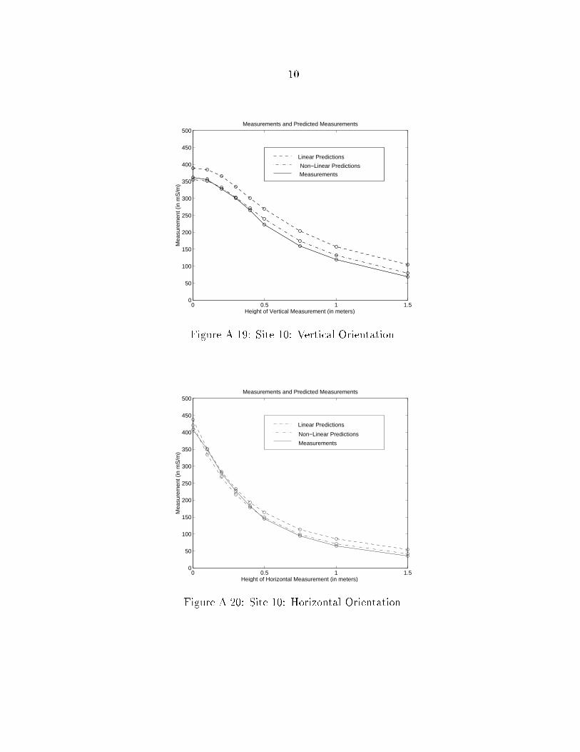
Observation � The nonlinear model almost always over predicts EM�
�� measurements� But it usually over predicts by less than ��� of the actual
measurements� In some cases the nonlinear model�s predictions are impressively
close to the actual measurements� Examples include sites �� �� �� and ���
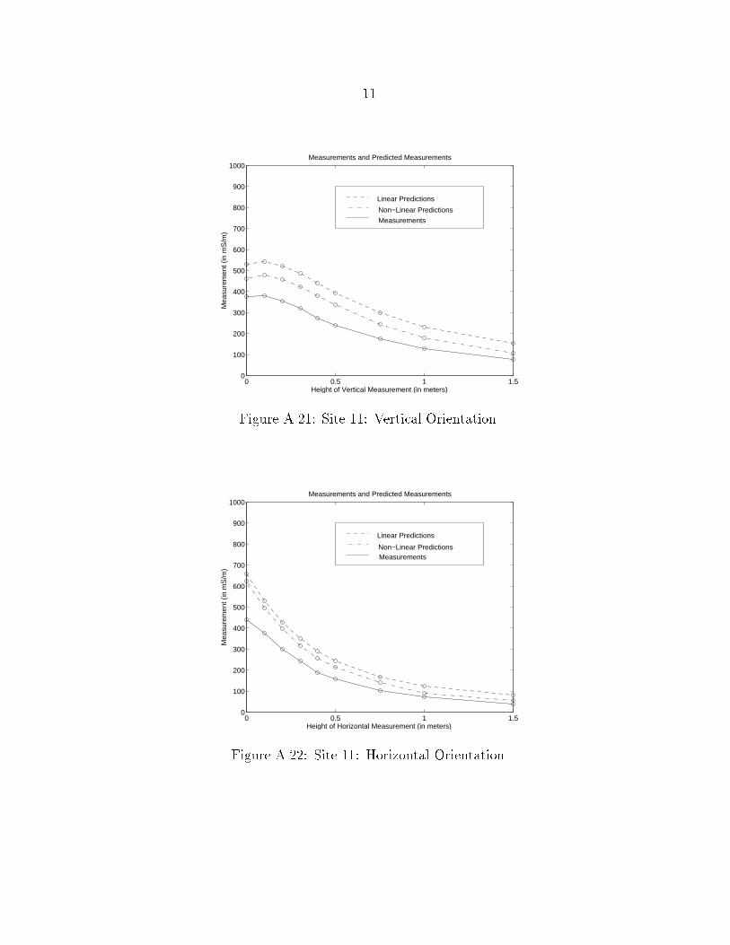
Observation � At sites with high soil conductivities� the nonlinear
model tends to make large improvements on the forward predictions� At sites
with low conductivities� the nonlinear model usually makes only subtle improve�
ments�
To demonstrate observation �� we will partition the �� sites into those
with �high� conductivities and those with �low� conductivities� The partition
will be based on the largest conductivity measurement� Comparing the set of
�� maximum conductivities� it is natural to de�ne a high conductivity site to
be a site with a maximum reading of at least ���mSm � A low conductivity site
will be any site with a maximum reading of under ���mSm � Refer to table ������
Finally consider an alternative partitioning of the �� sites� This will
be based on the extent to which the nonlinear model outperforms the linear
model� On site �� �� ��� ��� and ��� the nonlinear model makes modest improve
ments� This is generally consistent with observation � because � of the � sites
have low conductivities� An exception is site � which has been categorized as a
high conductivity site� In examining the measured conductivity pro�le ��gure
��
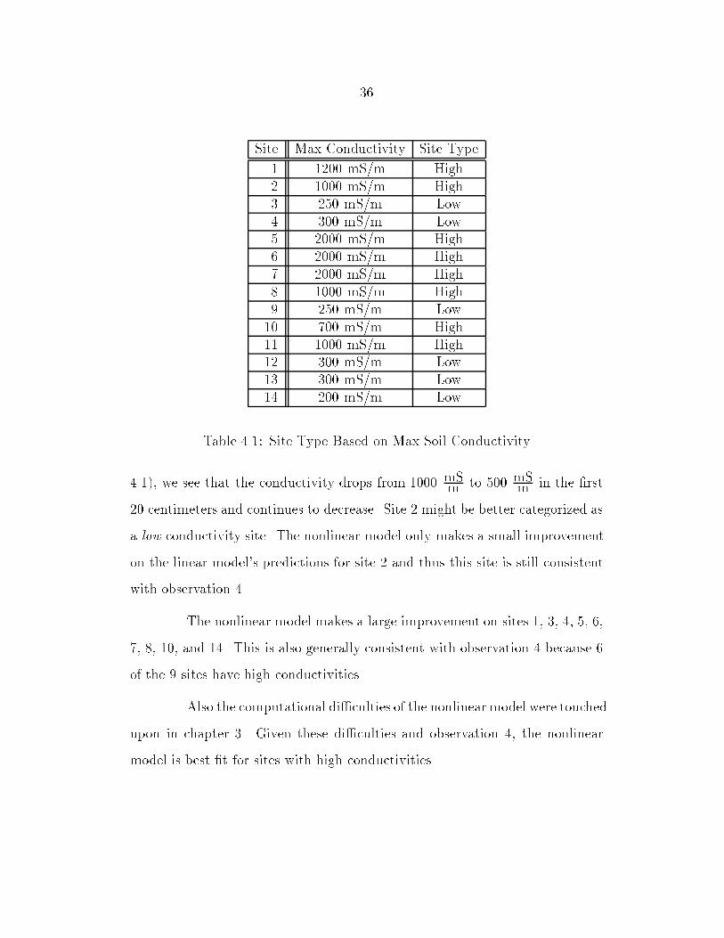
Site Max Conductivity Site Type
� ���� mS�m High� ���� mS�m High� ��� mS�m Low� ��� mS�m Low� ���� mS�m High� ���� mS�m High� ���� mS�m High� ���� mS�m High� ��� mS�m Low
�� ��� mS�m High�� ���� mS�m High�� ��� mS�m Low�� ��� mS�m Low�� ��� mS�m Low
Table ���� Site Type Based on Max Soil Conductivity
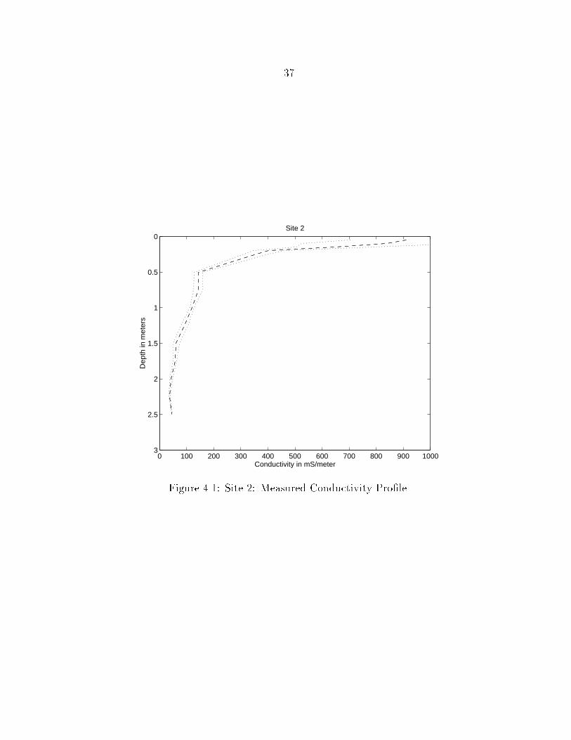
����� we see that the conductivity drops from ���� mSm to ��� mS
m in the �rst
�� centimeters and continues to decrease� Site � might be better categorized as
a low conductivity site� The nonlinear model only makes a small improvement
on the linear model�s predictions for site � and thus this site is still consistent
with observation ��
The nonlinear model makes a large improvement on sites �� �� �� �� ��
�� �� ��� and ��� This is also generally consistent with observation � because �
of the � sites have high conductivities�
Also the computational di�culties of the nonlinear model were touched
upon in chapter �� Given these di�culties and observation �� the nonlinear
model is best �t for sites with high conductivities�
��
0 100 200 300 400 500 600 700 800 900 1000
0
0.5
1
1.5
2
2.5
3
Conductivity in mS/meter
Dep
th in
met
ers
Site 2
Figure ���� Site �� Measured Conductivity Pro�le�
Chapter
Inverse Results
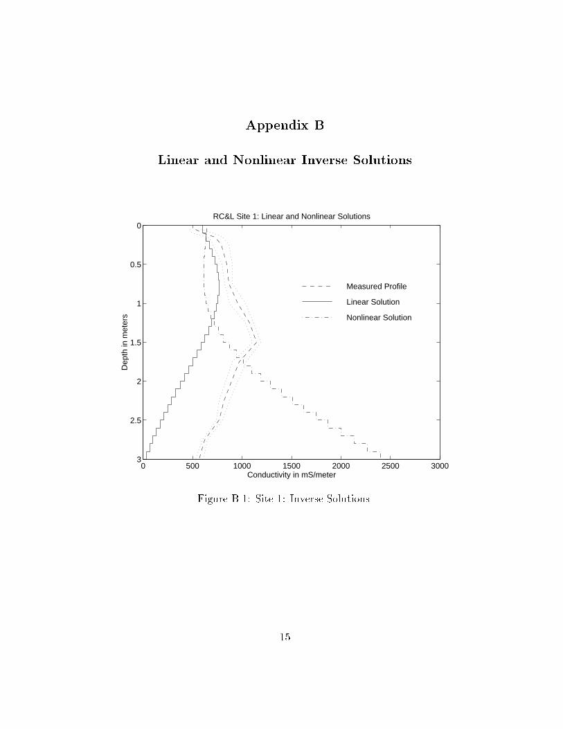
��� Discussion of Inverse Plots
The inverse problem has been solved for each of the �� Rhoades�
Corwin� and Lesch sites using each of the two models� Appendix B contains
one plot for each site� Each plot contains a solution for each model and the
average measured conductivity at each depth with one standard deviation bars�
The technical details of these runs were outlined in the previous chap
ter� It should be noted that the Lcurve criterion was used to pick the regu
larization parameter ��� Attempts to use crossvalidation on the linear model
were made� The resulting solutions were by no means better than the Lcurve
solutions� Given the computationally expensive nature of crossvalidation� ap
plication to the nonlinear model is currently infeasible� Also� an attempt to
use the discrepancy principle on the linear model was made� This attempt was
also not successful� The solution is far too sensitive to changes in the upper
bound of kK � dk��� The Lcurve method is inexpensive to implement and
relatively stable�
Chapter � partitioned the �� sites into high and low conductivity
pro�les� It was concluded that the nonlinear model was more appropriate
than the linear model for high conductivity sites� We will continue this line of
reasoning here�
��
��
Again take sites �� �� ��� ��� and �� to be low conductivity sites� For
sites �� ��� and �� the linear and nonlinear solutions are nearly identical� The
nonlinear solution for site �� is less regularized than the linear solution� It is
more regularized for site �� But for both sites the solution quality is similar�
Now consider the remaining sites� The quality of the solutions for
sites �� �� �� ��� and �� are nearly identical� The nonlinear solution for sites ��
�� and � are excellent whereas the linear solutions fails after ��� meters� Here
the nonlinear model is more sensitive than the linear model to lower depths�
This also will be discussed in the next section� These sites are interesting as
the measurements all increase with depth� Nonlinear success for site � is also
due in part to the second order regularization� This regularization is most
advantageous when a pro�le has little curvature�
Figure �B��� of the site � inverse solutions demonstrates an impor
tant point about the solution process� the choice of �� is critical� The linear
solution is able to pick up trends in the �rst ��� meters because it is somewhat
�underregularized� and allowed to bend� Perhaps with a good value of ���
the nonlinear models could yield an better result� For this site the nonlinear
Lcurve resulted in large �� resulting in a solution with no curvature�
Chapter �
Possible Explanations of Unexplained Behaviors
This discussion of in uences not included in these models has been
reserved for a separate chapter� Note that every in uence listed below could
potentially eect both forward and inverse calculations�
��� Semi�in�nite Layer
Both models assume a semiin�nite layer beginning at the � meter
mark� By semiin�nite we mean that the conductivity is uniform from � me
ters down toward the center of the earth� Some assumption on this conductivity
must be made for the forward predictions� The plots included in this paper
assume that the conductivity of the bottom layer is the �nal interpolated con
ductivity� A set of similar plots was created assuming this conductivity to be
zero� This had a large eect on the linear model�s predictions and a small
eect on the nonlinear model�s predictions� We conclude that the linear model
is sensitive to conductivities below � meters�
��� Magnetic Permeability
In the chapter � description of the nonlinear model� �i represented
the magnetic permeability of the ith layer of soil� Also �� was taken to be the
magnetic permeability of air� This study has consistently assumed that �i � ��
��
��
for all i� But for soils containing magnetic material such as magnetite this is
not the case� It is known� however� that very little of these materials existed
at the Rhoades� Corwin� and Lesch sites�
��� Discretization
Both models assume a vertical discretization of the soil pro�le� Though
this cannot be avoided in practice� it always induces some level of error�
�� Instrument Calibration
Calibration problems with the instruments used to collect the data
could aect the results� This could be the case with either the EM�� or the
MartekProbe�
��� Temperature E�ects
Soil conductivity is aected by temperature� There is always a certain
danger in invasive experimentation� The removal of top soil or side soils could
have an eect on ECa readings�
��� Vertical E�ects
Though the sensitivity of the instrument decays with depth� an ex
tremely high conductivity below ��� meters could aect results� A water table
could� for example� cause a sharp increase in conductivity� Second order regu
larization would have a di�cult time picking out the sharp increase� Perhaps
the solution would try to compensate by over predicting at depths directly
above the water table�
��
�� Depth Sensitivity
Both models have some di�culty inverting pro�les below ��� meters�
This sensitivity matter is a particular problem for the linear model� This is not
surprising� As shown by �gure����� the instrument is most sensitive to shallow
depths�
�� Lateral Homogeneity
Both models make an important assumption� that conductivity varies
only with depth� This assumption does not hold in practice� At nearly every
depth at nearly every site� there is considerable variability in the measured
ECa values� Furthermore at some sights there are strong lateral trends in ECa�
Though a thorough sensitivity analysis has not yet been conducted� it seems
reasonable that EM measurements would be sensitive to surface or subsurface
anomalies beyond the �� cm by �� cm square in which the ECa was actually
measured� A larger range of data is not currently available�
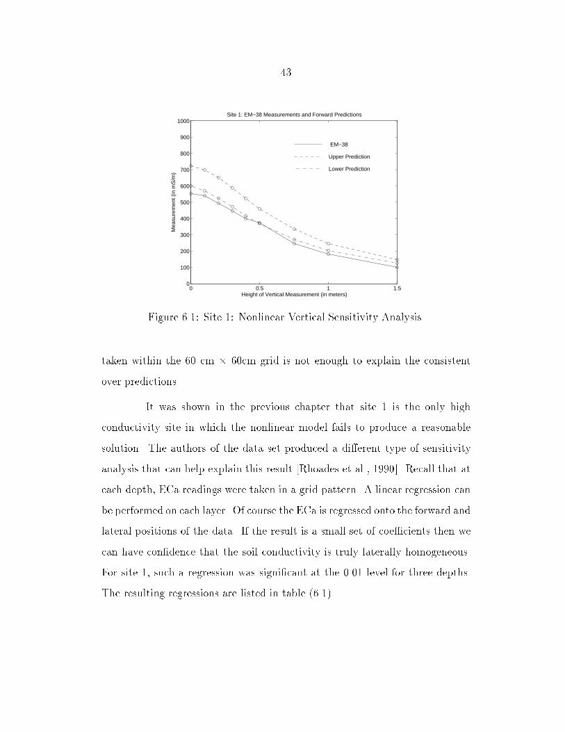
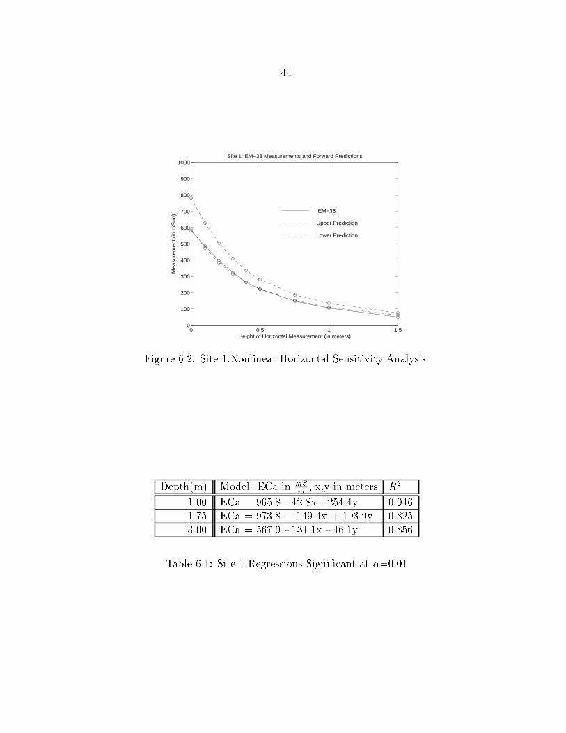
A forward sensitivity analysis can� however� be performed� Recall
that at each depth� � measurements were taken� Figures ����� and ����� depict
forward nonlinear predictions for site �� The dashed line represents forward
predictions using only the largest measured conductivity at each depth� Here
we use the conservative assumption that the semiin�nite layer is at the last
measured conductivity� The dash�dot line represents the predictions using only
the lowest conductivity at each depth� Here we use the liberal assumption that
the semiin�nite layer is � mS
m� In neither plot do the EM�� readings lie within
these predictions� It seems that lateral variability in the ECa measurements
��
0 0.5 1 1.50
100
200
300
400
500
600
700
800
900
1000
Height of Vertical Measurement (in meters)
Mea
sure
men
t (in
mS
/m)
Site 1: EM−38 Measurements and Forward Predictions
EM−38
Upper Prediction
Lower Prediction
Figure ���� Site �� Nonlinear Vertical Sensitivity Analysis�
taken within the �� cm ��cm grid is not enough to explain the consistent
over predictions�
It was shown in the previous chapter that site � is the only high
conductivity site in which the nonlinear model fails to produce a reasonable
solution� The authors of the data set produced a dierent type of sensitivity
analysis that can help explain this result �Rhoades et al�� ������ Recall that at
each depth� ECa readings were taken in a grid pattern� A linear regression can
be performed on each layer� Of course the ECa is regressed onto the forward and
lateral positions of the data� If the result is a small set of coe�cients then we
can have con�dence that the soil conductivity is truly laterally homogeneous�
For site �� such a regression was signi�cant at the ���� level for three depths�
The resulting regressions are listed in table ������
��
0 0.5 1 1.50
100
200
300
400
500
600
700
800
900
1000
Height of Horizontal Measurement (in meters)
Mea
sure
men
t (in
mS
/m)
Site 1: EM−38 Measurements and Forward Predictions
EM−38
Upper Prediction
Lower Prediction
Figure ���� Site ��Nonlinear Horizontal Sensitivity Analysis�
Depth�m� Model� ECa in mS
m� x�y in meters R�
���� ECa � ����� ����x �����y ��������� ECa � ����� � �����x � �����y ��������� ECa � ����� �����x ����y �����
Table ���� Site � Regressions Signi�cant at ������

��
For example� at ���� meters below the earth� a move of � meter in the
y direction could result in an ECa increase of almost ��� mS�m� With this sort
of change it is possible that varying conductivities outside of the measurement
grid could have a strong impact on the EM�� measurements and thus the
inverse solutions�
Chapter �
Summary and Conclusions
The EM�� inverse problem is only successfully solved as a least
squares problem when EM�� measurements can be accurately predicted from
a measured conductivity pro�le� With this in mind� an extensive eort to com
pare forward linear and nonlinear predictions has been made� It was found that
both models over predicted the EM�� measurements� The nonlinear model
without exception outperformed the linear model in forward predictions� The
dierence was substantial for sites with high soil conductivities� In fact� the
nonlinear model generally produced satisfactory results for our purposes�
In choosing a regularization parameter� the Lcurve principle should
be used� The discrepancy principle is too sensitive to estimations of � and
crossvalidation is too computationally expensive�
In some cases the nonlinear model does not outperform the linear
model� The linear model� on the other hand� only outperforms the nonlinear
model for site �� The general failure of both models on site � can be� however�
partially attributed to a lack of lateral homogeneity�
Considering the computational expense of solving the nonlinear model�
the linear model may be appropriate for low conductivities and for depths down
to ��� meters�
This study introduces a comparison of two models and an overview of
��

��
how they might be solved� External in uences are not completely understood�
Further research is needed to understand the in uences of lateral anomalies�
Perhaps the range of ECa readings could be extended to a ��� meter square and
a more thorough sensitivity analysis could be performed� Finally� this study
has inverted only one dimensional pro�les� Two and three dimensional models
are being examined �Alumbaugh et al�� ����� Newman and Alumbaugh� �����
Alumbaugh and Newman� ������
Appendix A
Forward Plots
0 0.5 1 1.50
100
200
300
400
500
600
700
800
900
1000Measurements and Predicted Measurements
Height of Vertical Measurement (in meters)
Mea
sure
men
t (in
mS
/m)
Linear PredictionsNon−Linear Predictions
Measurements
Figure A��� Site �� Vertical Orientation�
0 0.5 1 1.50
100
200
300
400
500
600
700
800
900
1000Measurements and Predicted Measurements
Height of Horizontal Measurement (in meters)
Mea
sure
men
t (in
mS
/m)
Linear Predictions
Non−Linear Predictions
Measurements
Figure A��� Site �� Horizontal Orientation�
�

�
0 0.5 1 1.50
50
100
150
200
250
300
350
400
450
500Measurements and Predicted Measurements
Height of Vertical Measurement (in meters)
Mea
sure
men
t (in
mS
/m)
Linear Predictions
Non−Linear PredictionsMeasurements
Figure A��� Site �� Vertical Orientation�
0 0.5 1 1.50
50
100
150
200
250
300
350
400
450
500Measurements and Predicted Measurements
Height of Horizontal Measurement (in meters)
Mea
sure
men
t (in
mS
/m)
Linear Predictions
Non−Linear Predictions
Measurements
Figure A��� Site �� Horizontal Orientation�
�
0 0.5 1 1.50
10
20
30
40
50
60
70
80
90
100Measurements and Predicted Measurements
Height of Vertical Measurement (in meters)
Mea
sure
men
t (in
mS
/m)
Linear Predictions
Non−Linear Predictions
Measurements
Figure A��� Site �� Vertical Orientation�
0 0.5 1 1.50
10
20
30
40
50
60
70
80
90
100Measurements and Predicted Measurements
Height of Horizontal Measurement (in meters)
Mea
sure
men
t (in
mS
/m)
Linear Predictions
Non−Linear Predictions
Measurements
Figure A��� Site �� Horizontal Orientation�
�
0 0.5 1 1.50
20
40
60
80
100
120
140
160
180
200Measurements and Predicted Measurements
Height of Vertical Measurement (in meters)
Mea
sure
men
t (in
mS
/m)
Linear Predictions
Non−Linear Predictions
Measurements
Figure A��� Site �� Vertical Orientation�
0 0.5 1 1.50
20
40
60
80
100
120
140
160
180
200Measurements and Predicted Measurements
Height of Horizontal Measurement (in meters)
Mea
sure
men
t (in
mS
/m)
Linear Predictions
Non−Linear Predictions
Measurements
Figure A��� Site �� Horizontal Orientation�
�
0 0.5 1 1.50
500
1000
1500Measurements and Predicted Measurements
Height of Vertical Measurement (in meters)
Mea
sure
men
t (in
mS
/m)
Linear Predictions
Non−Linear PredictionsMeasurements
Figure A��� Site �� Vertical Orientation�
0 0.5 1 1.50
500
1000
1500Measurements and Predicted Measurements
Height of Horizontal Measurement (in meters)
Mea
sure
men
t (in
mS
/m)
Linear Predictions
Non−Linear PredictionsMeasurements
Figure A���� Site �� Horizontal Orientation�
�
0 0.5 1 1.50
100
200
300
400
500
600
700
800
900
1000Measurements and Predicted Measurements
Height of Vertical Measurement (in meters)
Mea
sure
men
t (in
mS
/m)
Linear PredictionsNon−Linear Predictions
Measurements
Figure A���� Site �� Vertical Orientation�
0 0.5 1 1.50
100
200
300
400
500
600
700
800
900
1000Measurements and Predicted Measurements
Height of Horizontal Measurement (in meters)
Mea
sure
men
t (in
mS
/m)
Linear Predictions
Non−Linear PredictionsMeasurements
Figure A���� Site �� Horizontal Orientation�
�
0 0.5 1 1.50
100
200
300
400
500
600
700
800
900
1000Measurements and Predicted Measurements
Height of Vertical Measurement (in meters)
Mea
sure
men
t (in
mS
/m)
Linear Predictions
Non−Linear Predictions
Measurements
Figure A���� Site �� Vertical Orientation�
0 0.5 1 1.50
100
200
300
400
500
600
700
800
900
1000Measurements and Predicted Measurements
Height of Horizontal Measurement (in meters)
Mea
sure
men
t (in
mS
/m)
Linear Predictions
Non−Linear Predictions
Measurements
Figure A���� Site �� Horizontal Orientation�
�
0 0.5 1 1.50
50
100
150
200
250
300
350
400
450
500Measurements and Predicted Measurements
Height of Vertical Measurement (in meters)
Mea
sure
men
t (in
mS
/m)
Linear Predictions
Non−Linear Predictions
Measurements
Figure A���� Site �� Vertical Orientation�
0 0.5 1 1.50
50
100
150
200
250
300
350
400
450
500Measurements and Predicted Measurements
Height of Horizontal Measurement (in meters)
Mea
sure
men
t (in
mS
/m)
Linear Predictions
Non−Linear Predictions
Measurements
Figure A���� Site �� Horizontal Orientation�
�
0 0.5 1 1.50
50
100
150
200
250Measurements and Predicted Measurements
Height of Vertical Measurement (in meters)
Mea
sure
men
t (in
mS
/m)
Linear Predictions
Non−Linear Predictions
Measurements
Figure A���� Site �� Vertical Orientation�
0 0.5 1 1.50
50
100
150
200
250Measurements and Predicted Measurements
Height of Horizontal Measurement (in meters)
Mea
sure
men
t (in
mS
/m)
Linear Predictions
Non−Linear PredictionsMeasurements
Figure A���� Site �� Horizontal Orientation�
��
0 0.5 1 1.50
50
100
150
200
250
300
350
400
450
500Measurements and Predicted Measurements
Height of Vertical Measurement (in meters)
Mea
sure
men
t (in
mS
/m)
Linear Predictions
Non−Linear Predictions
Measurements
Figure A���� Site ��� Vertical Orientation�
0 0.5 1 1.50
50
100
150
200
250
300
350
400
450
500Measurements and Predicted Measurements
Height of Horizontal Measurement (in meters)
Mea
sure
men
t (in
mS
/m)
Linear Predictions
Non−Linear Predictions
Measurements
Figure A���� Site ��� Horizontal Orientation�
��
0 0.5 1 1.50
100
200
300
400
500
600
700
800
900
1000Measurements and Predicted Measurements
Height of Vertical Measurement (in meters)
Mea
sure
men
t (in
mS
/m)
Linear Predictions
Non−Linear Predictions
Measurements
Figure A���� Site ��� Vertical Orientation�
0 0.5 1 1.50
100
200
300
400
500
600
700
800
900
1000Measurements and Predicted Measurements
Height of Horizontal Measurement (in meters)
Mea
sure
men
t (in
mS
/m)
Linear Predictions
Non−Linear PredictionsMeasurements
Figure A���� Site ��� Horizontal Orientation�
��
0 0.5 1 1.50
20
40
60
80
100
120
140
160
180
200Measurements and Predicted Measurements
Height of Vertical Measurement (in meters)
Mea
sure
men
t (in
mS
/m)
Linear Predictions
Non−Linear Predictions
Measurements
Figure A���� Site ��� Vertical Orientation�
0 0.5 1 1.50
20
40
60
80
100
120
140
160
180
200Measurements and Predicted Measurements
Height of Horizontal Measurement (in meters)
Mea
sure
men
t (in
mS
/m)
Linear Predictions
Non−Linear Predictions
Measurements
Figure A���� Site ��� Horizontal Orientation�
��
0 0.5 1 1.50
50
100
150
200
250
300
350
400
450
500Measurements and Predicted Measurements
Height of Vertical Measurement (in meters)
Mea
sure
men
t (in
mS
/m)
Linear Predictions
Non−Linear Predictions
Measurements
Figure A���� Site ��� Vertical Orientation�
0 0.5 1 1.50
50
100
150
200
250
300
350
400
450
500Measurements and Predicted Measurements
Height of Horizontal Measurement (in meters)
Mea
sure
men
t (in
mS
/m)
Linear Predictions
Non−Linear PredictionsMeasurements
Figure A���� Site ��� Horizontal Orientation�
��
0 0.5 1 1.50
10
20
30
40
50
60
70
80
90
100Measurements and Predicted Measurements
Height of Vertical Measurement (in meters)
Mea
sure
men
t (in
mS
/m)
Linear Predictions
Non−Linear Predictions
Measurements
Figure A���� Site ��� Vertical Orientation�
0 0.5 1 1.50
10
20
30
40
50
60
70
80
90
100Measurements and Predicted Measurements
Height of Horizontal Measurement (in meters)
Mea
sure
men
t (in
mS
/m)
Linear Predictions
Non−Linear PredictionsMeasurements
Figure A���� Site ��� Horizontal Orientation�
Appendix B
Linear and Nonlinear Inverse Solutions
0 500 1000 1500 2000 2500 3000
0
0.5
1
1.5
2
2.5
3
Conductivity in mS/meter
Dep
th in
met
ers
RC&L Site 1: Linear and Nonlinear Solutions
Nonlinear Solution
Linear Solution
Measured Profile
Figure B��� Site �� Inverse Solutions�
��
��
0 500 1000 1500
0
0.5
1
1.5
2
2.5
3
Conductivity in mS/meter
Dep
th in
met
ers
RC&L Site 2: Linear and Nonlinear Solutions
Nonlinear Solution
Linear Solution
Measured Profile
Figure B��� Site �� Inverse Solutions�
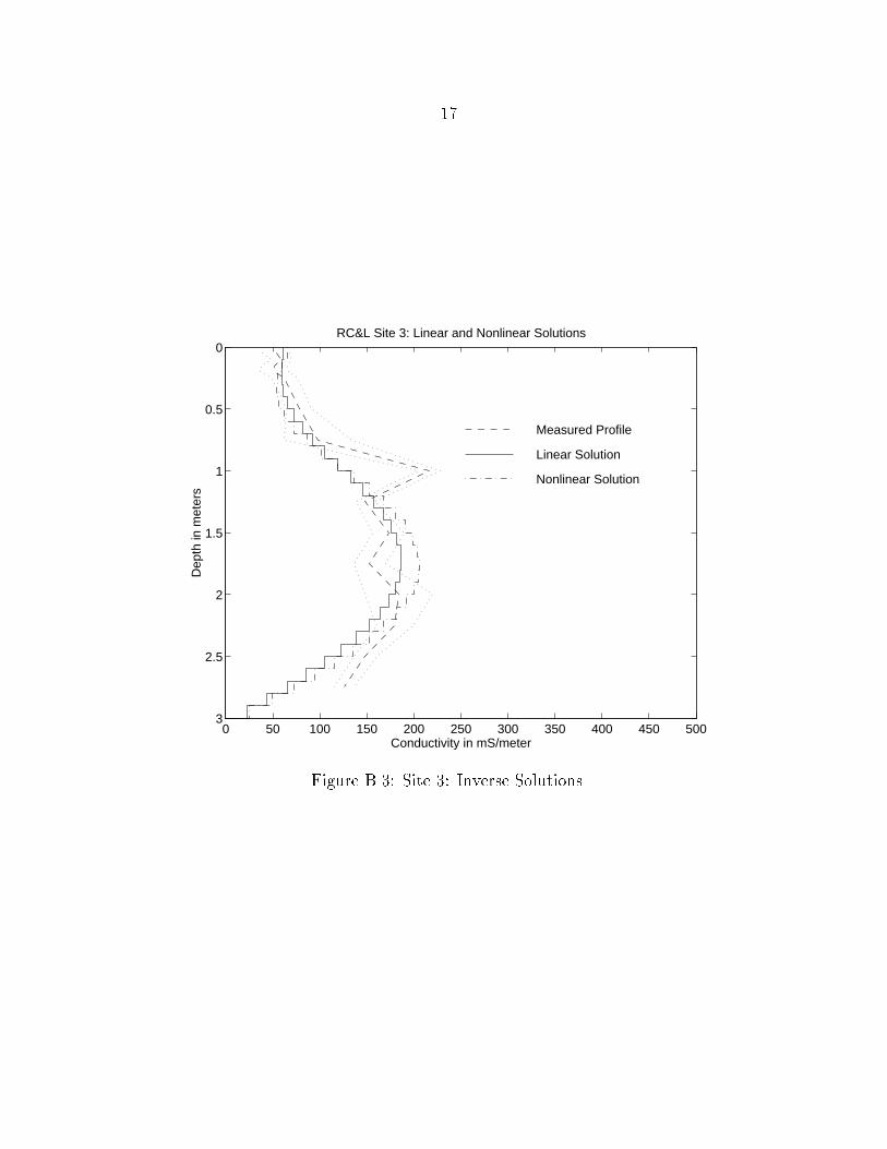
��
0 50 100 150 200 250 300 350 400 450 500
0
0.5
1
1.5
2
2.5
3
Conductivity in mS/meter
Dep
th in
met
ers
RC&L Site 3: Linear and Nonlinear Solutions
Nonlinear Solution
Linear Solution
Measured Profile
Figure B��� Site �� Inverse Solutions�
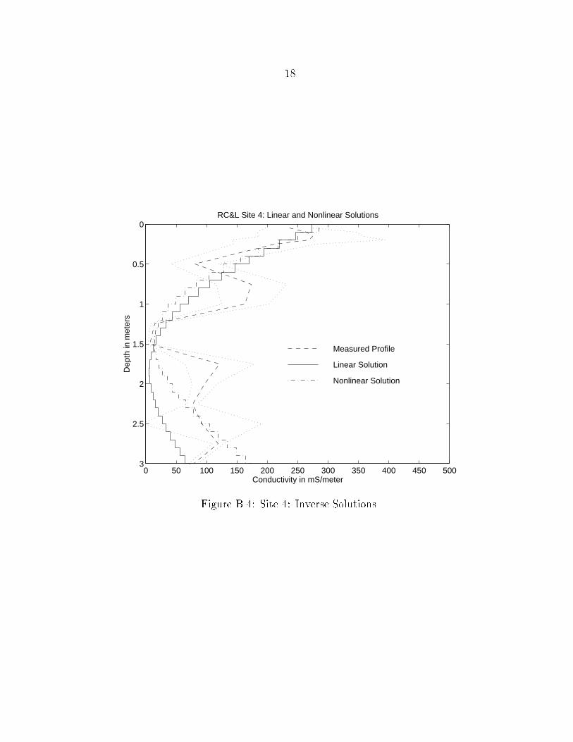
��
0 50 100 150 200 250 300 350 400 450 500
0
0.5
1
1.5
2
2.5
3
Conductivity in mS/meter
Dep
th in
met
ers
RC&L Site 4: Linear and Nonlinear Solutions
Nonlinear Solution
Linear Solution
Measured Profile
Figure B��� Site �� Inverse Solutions�
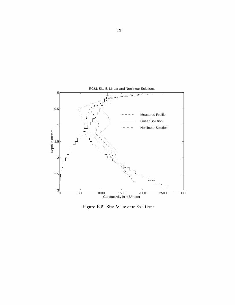
��
0 500 1000 1500 2000 2500 3000
0
0.5
1
1.5
2
2.5
3
Conductivity in mS/meter
Dep
th in
met
ers
RC&L Site 5: Linear and Nonlinear Solutions
Nonlinear Solution
Linear Solution
Measured Profile
Figure B��� Site �� Inverse Solutions�
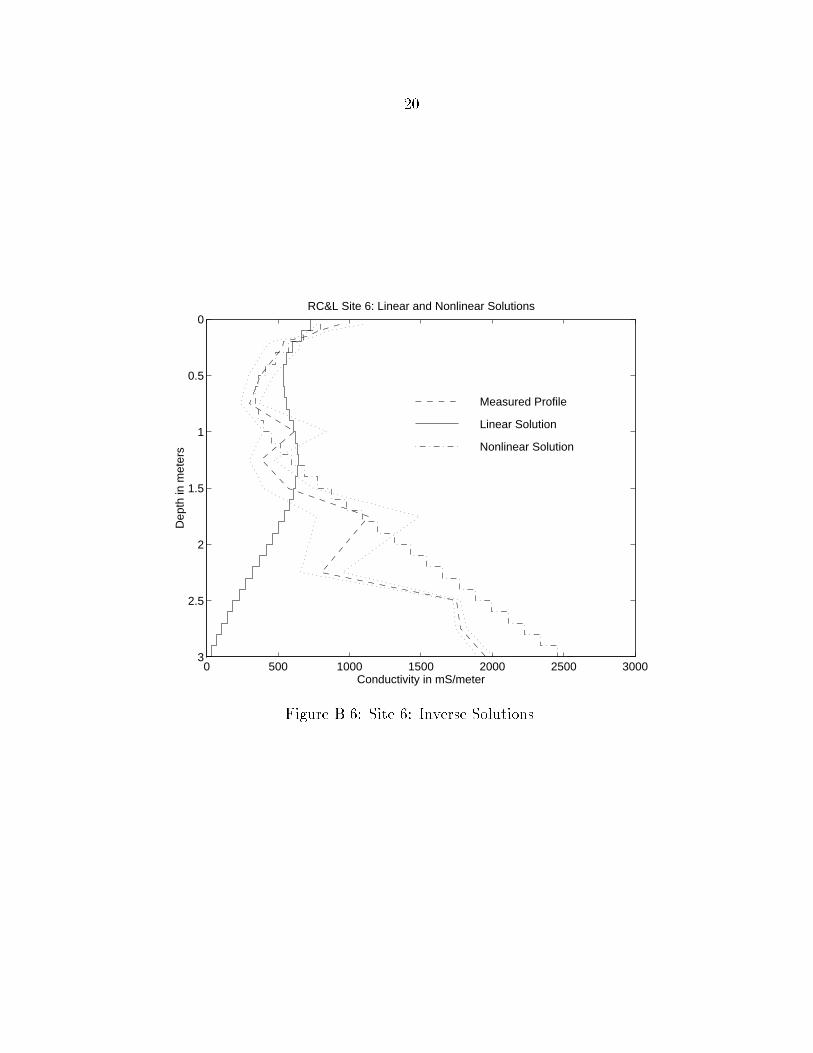
��
0 500 1000 1500 2000 2500 3000
0
0.5
1
1.5
2
2.5
3
Conductivity in mS/meter
Dep
th in
met
ers
RC&L Site 6: Linear and Nonlinear Solutions
Nonlinear Solution
Linear Solution
Measured Profile
Figure B��� Site �� Inverse Solutions�
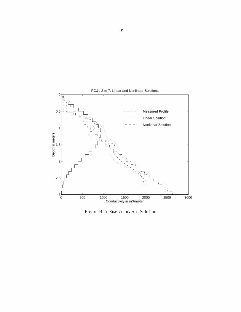
��
0 500 1000 1500 2000 2500 3000
0
0.5
1
1.5
2
2.5
3
Conductivity in mS/meter
Dep
th in
met
ers
RC&L Site 7: Linear and Nonlinear Solutions
Nonlinear Solution
Linear Solution
Measured Profile
Figure B��� Site �� Inverse Solutions�
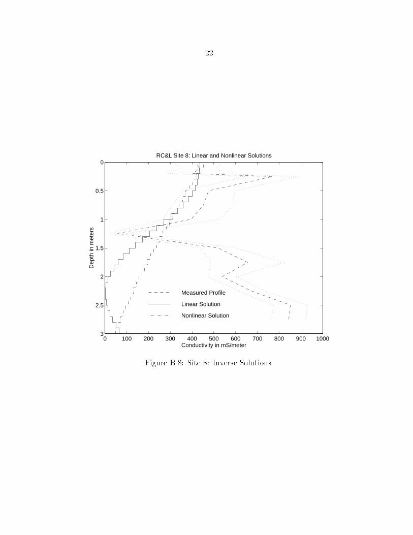
��
0 100 200 300 400 500 600 700 800 900 1000
0
0.5
1
1.5
2
2.5
3
Conductivity in mS/meter
Dep
th in
met
ers
RC&L Site 8: Linear and Nonlinear Solutions
Nonlinear Solution
Linear Solution
Measured Profile
Figure B��� Site �� Inverse Solutions�
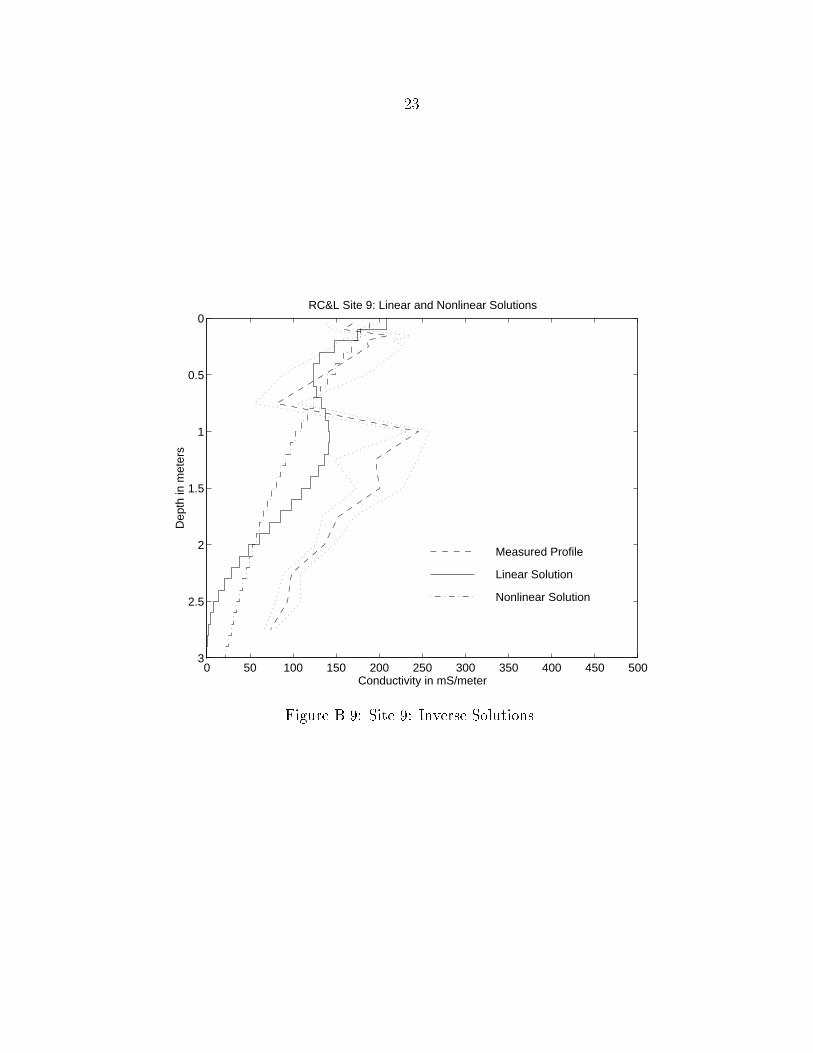
��
0 50 100 150 200 250 300 350 400 450 500
0
0.5
1
1.5
2
2.5
3
Conductivity in mS/meter
Dep
th in
met
ers
RC&L Site 9: Linear and Nonlinear Solutions
Nonlinear Solution
Linear Solution
Measured Profile
Figure B��� Site �� Inverse Solutions�
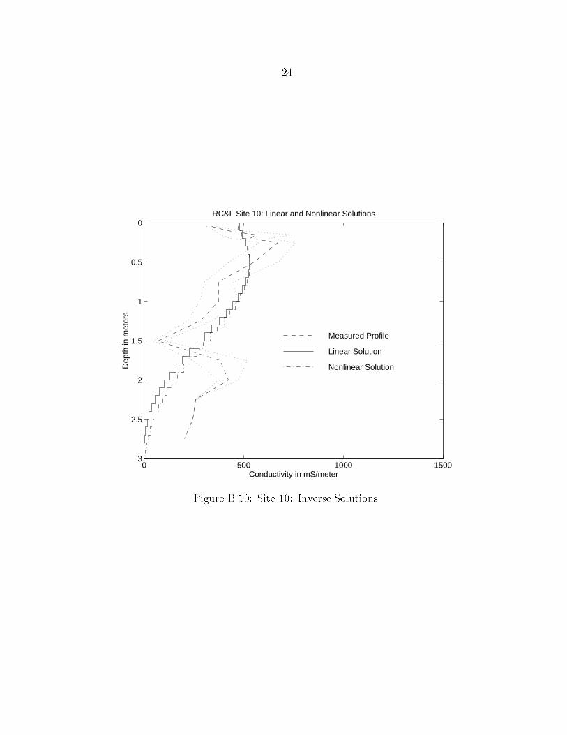
��
0 500 1000 1500
0
0.5
1
1.5
2
2.5
3
Conductivity in mS/meter
Dep
th in
met
ers
RC&L Site 10: Linear and Nonlinear Solutions
Nonlinear Solution
Linear Solution
Measured Profile
Figure B���� Site ��� Inverse Solutions�
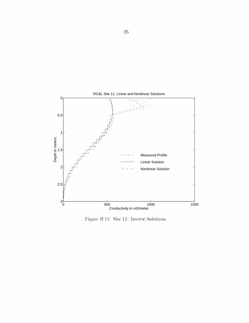
��
0 500 1000 1500
0
0.5
1
1.5
2
2.5
3
Conductivity in mS/meter
Dep
th in
met
ers
RC&L Site 11: Linear and Nonlinear Solutions
Nonlinear Solution
Linear Solution
Measured Profile
Figure B���� Site ��� Inverse Solutions�
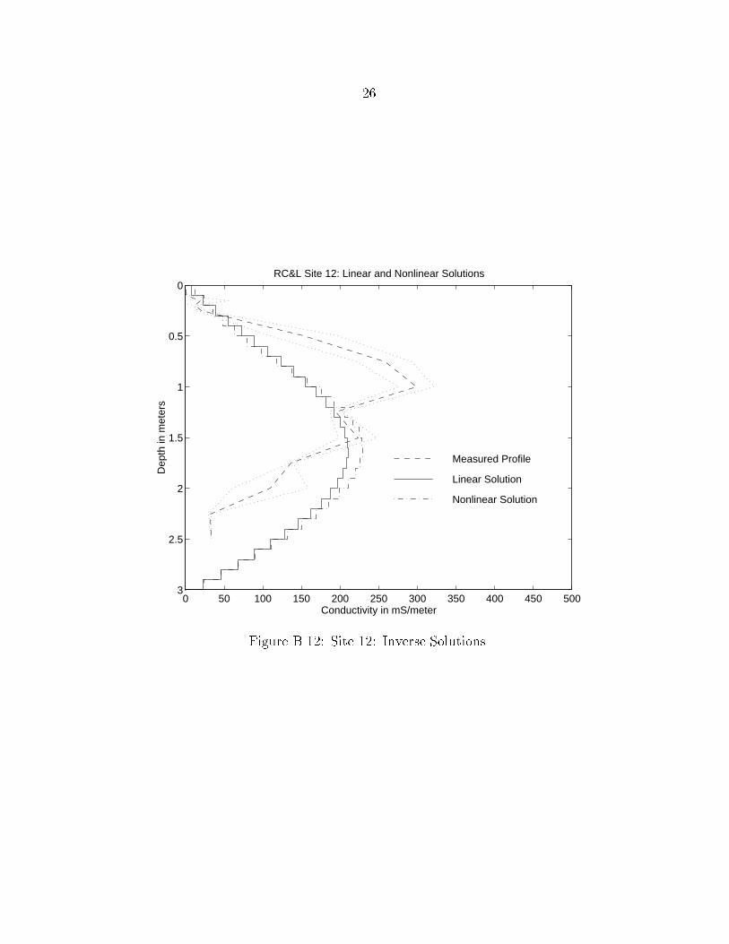
��
0 50 100 150 200 250 300 350 400 450 500
0
0.5
1
1.5
2
2.5
3
Conductivity in mS/meter
Dep
th in
met
ers
RC&L Site 12: Linear and Nonlinear Solutions
Nonlinear Solution
Linear Solution
Measured Profile
Figure B���� Site ��� Inverse Solutions�
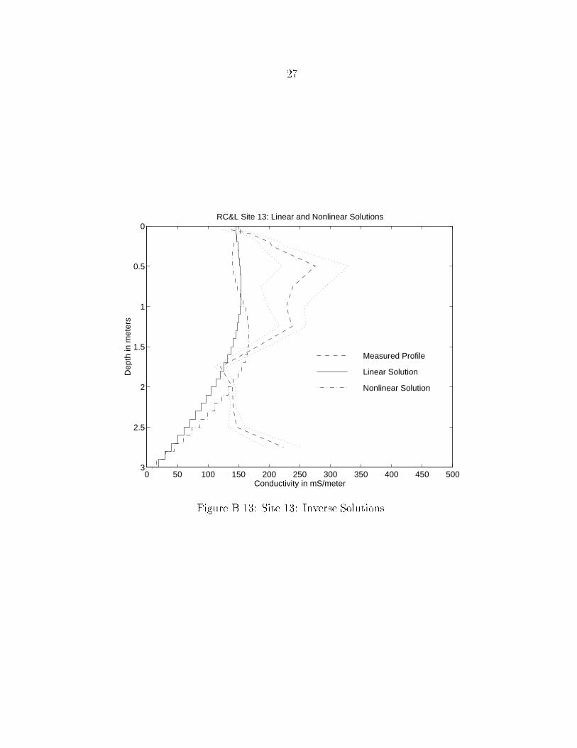
��
0 50 100 150 200 250 300 350 400 450 500
0
0.5
1
1.5
2
2.5
3
Conductivity in mS/meter
Dep
th in
met
ers
RC&L Site 13: Linear and Nonlinear Solutions
Nonlinear Solution
Linear Solution
Measured Profile
Figure B���� Site ��� Inverse Solutions�
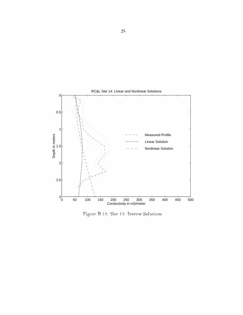
��
0 50 100 150 200 250 300 350 400 450 500
0
0.5
1
1.5
2
2.5
3
Conductivity in mS/meter
Dep
th in
met
ers
RC&L Site 14: Linear and Nonlinear Solutions
Nonlinear Solution
Linear Solution
Measured Profile
Figure B���� Site ��� Inverse Solutions�
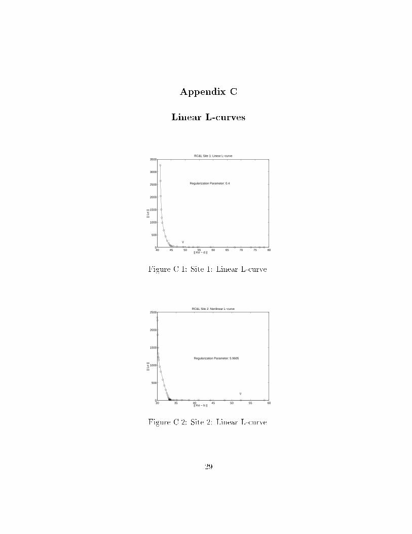
Appendix C
Linear L�curves
40 45 50 55 60 65 70 75 800
500
1000
1500
2000
2500
3000
3500RC&L Site 1: Linear L−curve
|| Kσ − d ||
|| Lσ
||
Regularization Parameter: 0.4
\/
Figure C��� Site �� Linear Lcurve�
30 35 40 45 50 55 600
500
1000
1500
2000
2500RC&L Site 2: Nonlinear L−curve
|| Kσ − b ||
|| Lσ
||
Regularization Parameter: 5.9605
\/
Figure C��� Site �� Linear Lcurve�
��
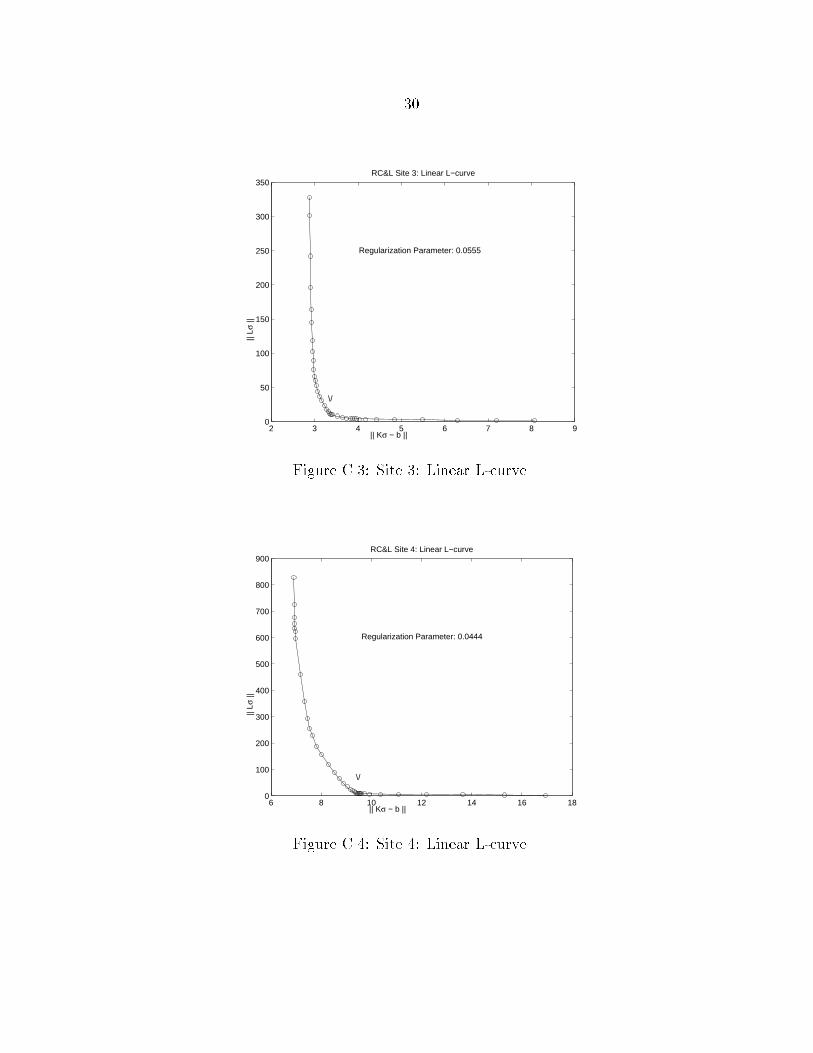
��
2 3 4 5 6 7 8 90
50
100
150
200
250
300
350RC&L Site 3: Linear L−curve
|| Kσ − b ||
|| Lσ
||
\/
Regularization Parameter: 0.0555
Figure C��� Site �� Linear Lcurve�
6 8 10 12 14 16 180
100
200
300
400
500
600
700
800
900RC&L Site 4: Linear L−curve
|| Kσ − b ||
|| Lσ
||
\/
Regularization Parameter: 0.0444
Figure C��� Site �� Linear Lcurve�
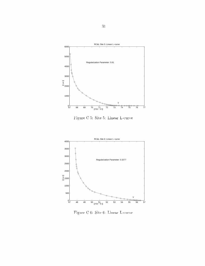
��
67 68 69 70 71 72 73 74 75 76 770
1000
2000
3000
4000
5000
6000RC&L Site 5: Linear L−curve
|| Kσ − d ||
|| Lσ
||Regularization Parameter: 0.61
\/
Figure C��� Site �� Linear Lcurve�
47 48 49 50 51 52 53 54 55 56 570
500
1000
1500
2000
2500
3000
3500
4000RC&L Site 6: Linear L−curve
|| Kσ − b ||
|| Lσ
||
\/
Regularization Parameter: 0.3277
Figure C��� Site �� Linear Lcurve�
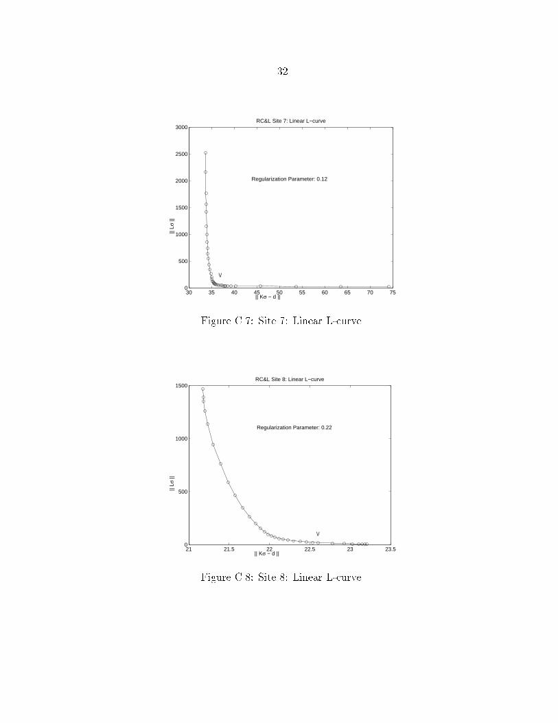
��
30 35 40 45 50 55 60 65 70 750
500
1000
1500
2000
2500
3000RC&L Site 7: Linear L−curve
|| Kσ − d ||
|| Lσ
||Regularization Parameter: 0.12
\/
Figure C��� Site �� Linear Lcurve�
21 21.5 22 22.5 23 23.50
500
1000
1500RC&L Site 8: Linear L−curve
|| Kσ − d ||
|| Lσ
||
Regularization Parameter: 0.22
\/
Figure C��� Site �� Linear Lcurve�
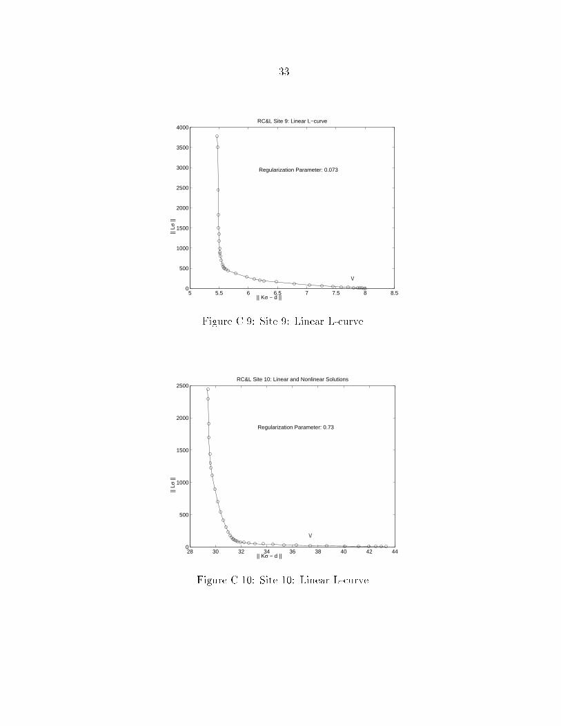
��
5 5.5 6 6.5 7 7.5 8 8.50
500
1000
1500
2000
2500
3000
3500
4000RC&L Site 9: Linear L−curve
|| Kσ − d ||
|| Lσ
||Regularization Parameter: 0.073
\/
Figure C��� Site �� Linear Lcurve�
28 30 32 34 36 38 40 42 440
500
1000
1500
2000
2500RC&L Site 10: Linear and Nonlinear Solutions
|| Kσ − d ||
|| Lσ
||
Regularization Parameter: 0.73
\/
Figure C���� Site ��� Linear Lcurve�
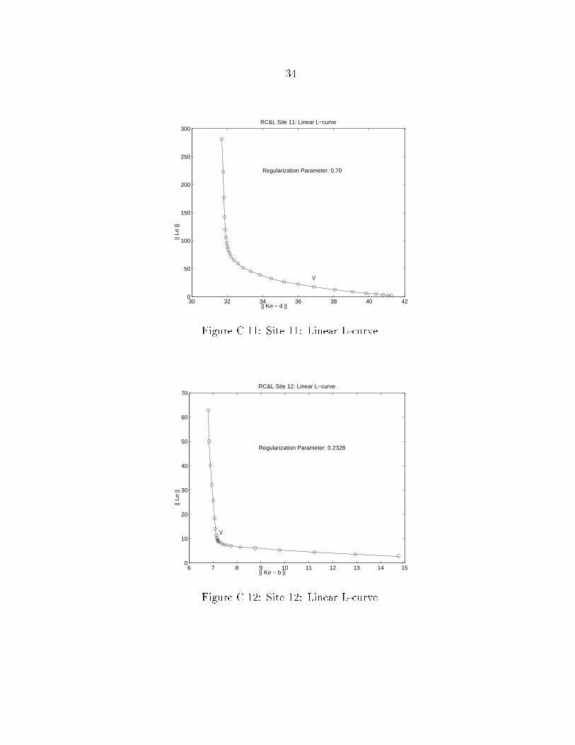
��
30 32 34 36 38 40 420
50
100
150
200
250
300RC&L Site 11: Linear L−curve
|| Kσ − d ||
|| Lσ
||Regularization Parameter: 0.70
\/
Figure C���� Site ��� Linear Lcurve�
6 7 8 9 10 11 12 13 14 150
10
20
30
40
50
60
70RC&L Site 12: Linear L−curve
|| Kσ − b ||
|| Lσ
||
Regularization Parameter: 0.2328
\/
Figure C���� Site ��� Linear Lcurve�
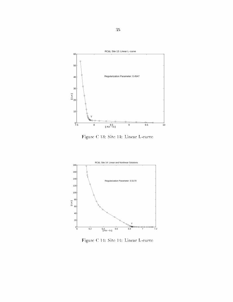
��
7.5 8 8.5 9 9.5 100
10
20
30
40
50
60RC&L Site 13: Linear L−curve
|| Kσ − b ||
|| Lσ
||
\/
Regularization Parameter: 0.4547
Figure C���� Site ��� Linear Lcurve�
6 6.2 6.4 6.6 6.8 7 7.20
20
40
60
80
100
120
140
160
180RC&L Site 14: Linear and Nonlinear Solutions
|| Kσ − b ||
|| Lσ
||
Regularization Parameter: 0.5170
\/
Figure C���� Site ��� Linear Lcurve�
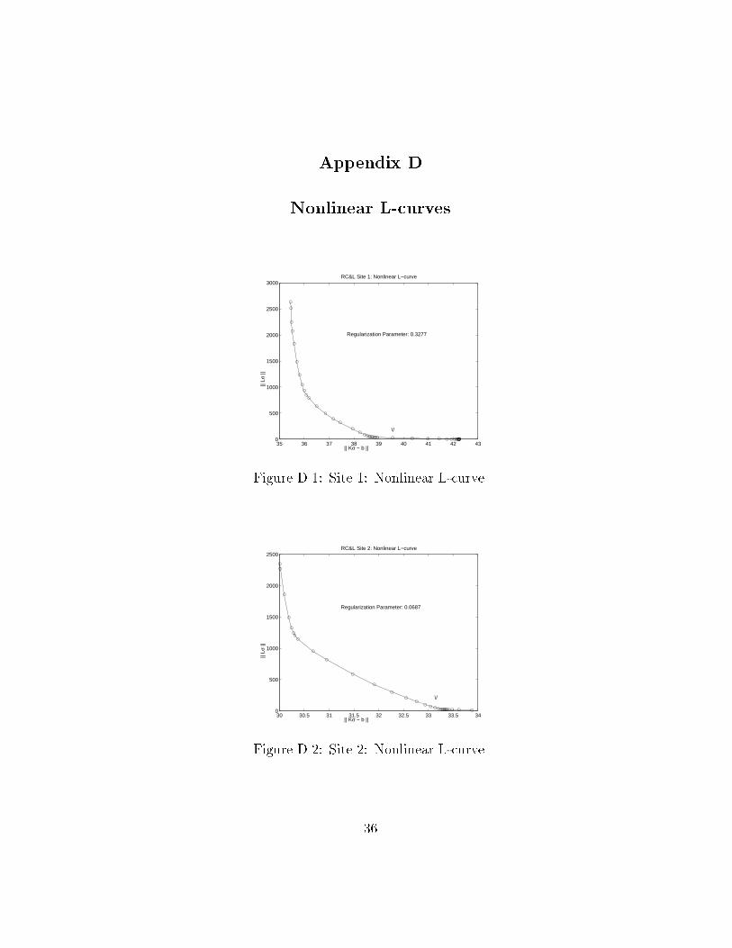
Appendix D
Nonlinear L�curves
35 36 37 38 39 40 41 42 430
500
1000
1500
2000
2500
3000RC&L Site 1: Nonlinear L−curve
|| Kσ − b ||
|| Lσ
||
\/
Regularization Parameter: 0.3277
Figure D��� Site �� Nonlinear Lcurve�
30 30.5 31 31.5 32 32.5 33 33.5 340
500
1000
1500
2000
2500RC&L Site 2: Nonlinear L−curve
|| Kσ − b ||
|| Lσ
||
\/
Regularization Parameter: 0.0687
Figure D��� Site �� Nonlinear Lcurve�
��
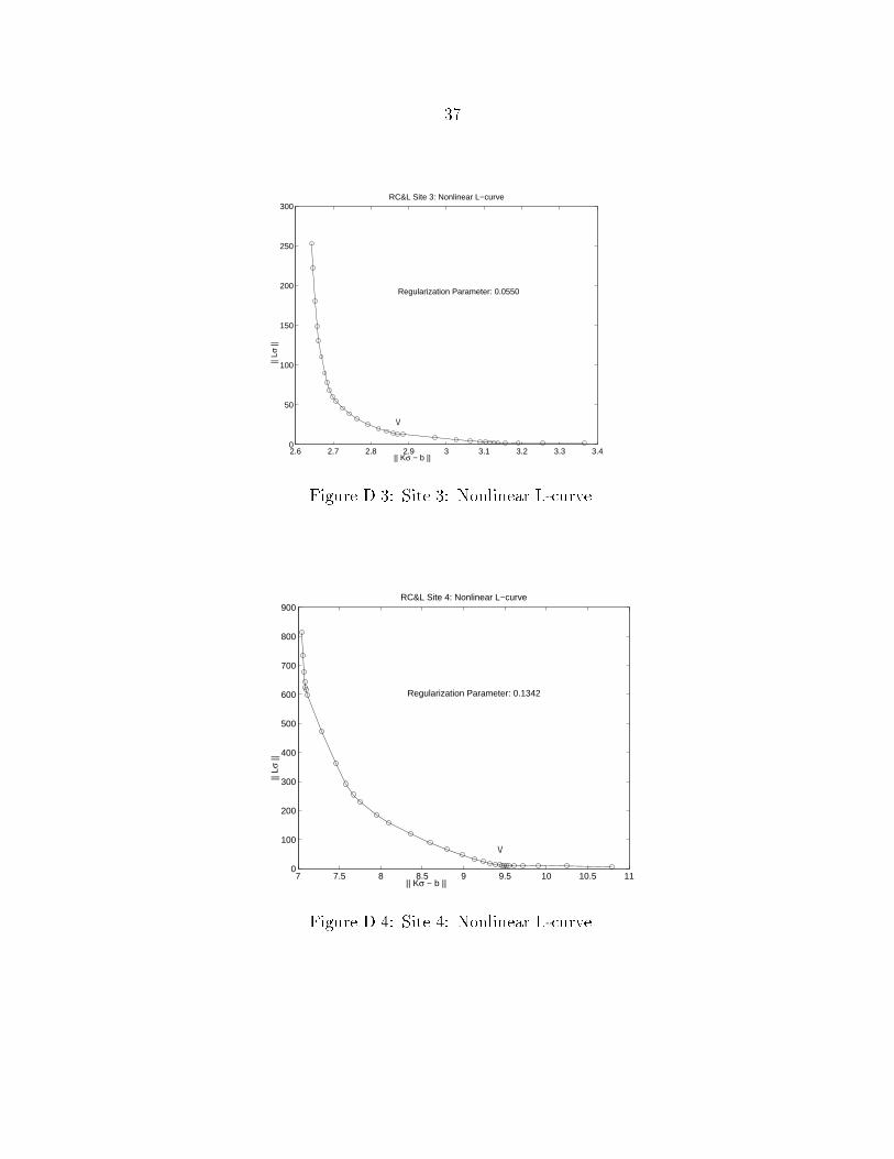
��
2.6 2.7 2.8 2.9 3 3.1 3.2 3.3 3.40
50
100
150
200
250
300RC&L Site 3: Nonlinear L−curve
|| Kσ − b ||
|| Lσ
||
\/
Regularization Parameter: 0.0550
Figure D��� Site �� Nonlinear Lcurve�
7 7.5 8 8.5 9 9.5 10 10.5 110
100
200
300
400
500
600
700
800
900RC&L Site 4: Nonlinear L−curve
|| Kσ − b ||
|| Lσ
||
\/
Regularization Parameter: 0.1342
Figure D��� Site �� Nonlinear Lcurve�
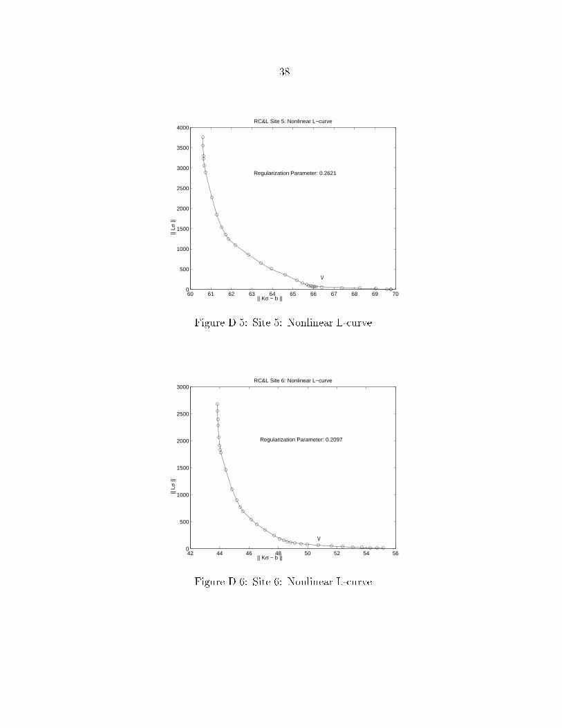
��
60 61 62 63 64 65 66 67 68 69 700
500
1000
1500
2000
2500
3000
3500
4000RC&L Site 5: Nonlinear L−curve
|| Kσ − b ||
|| Lσ
||
\/
Regularization Parameter: 0.2621
Figure D��� Site �� Nonlinear Lcurve�
42 44 46 48 50 52 54 560
500
1000
1500
2000
2500
3000RC&L Site 6: Nonlinear L−curve
|| Kσ − b ||
|| Lσ
||
\/
Regularization Parameter: 0.2097
Figure D��� Site �� Nonlinear Lcurve�
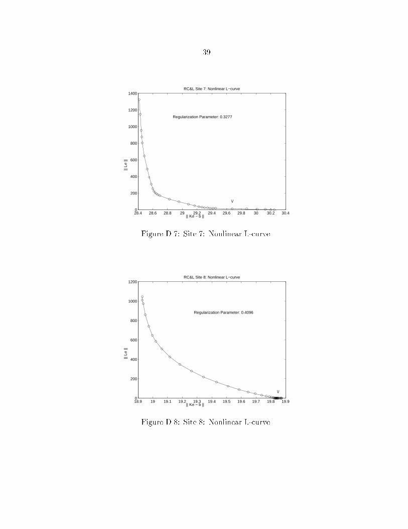
��
28.4 28.6 28.8 29 29.2 29.4 29.6 29.8 30 30.2 30.40
200
400
600
800
1000
1200
1400RC&L Site 7: Nonlinear L−curve
|| Kσ − b ||
|| Lσ
||
Regularization Parameter: 0.3277
\/
Figure D��� Site �� Nonlinear Lcurve�
18.9 19 19.1 19.2 19.3 19.4 19.5 19.6 19.7 19.8 19.90
200
400
600
800
1000
1200RC&L Site 8: Nonlinear L−curve
|| Kσ − b ||
|| Lσ
||
Regularization Parameter: 0.4096
\/
Figure D��� Site �� Nonlinear Lcurve�
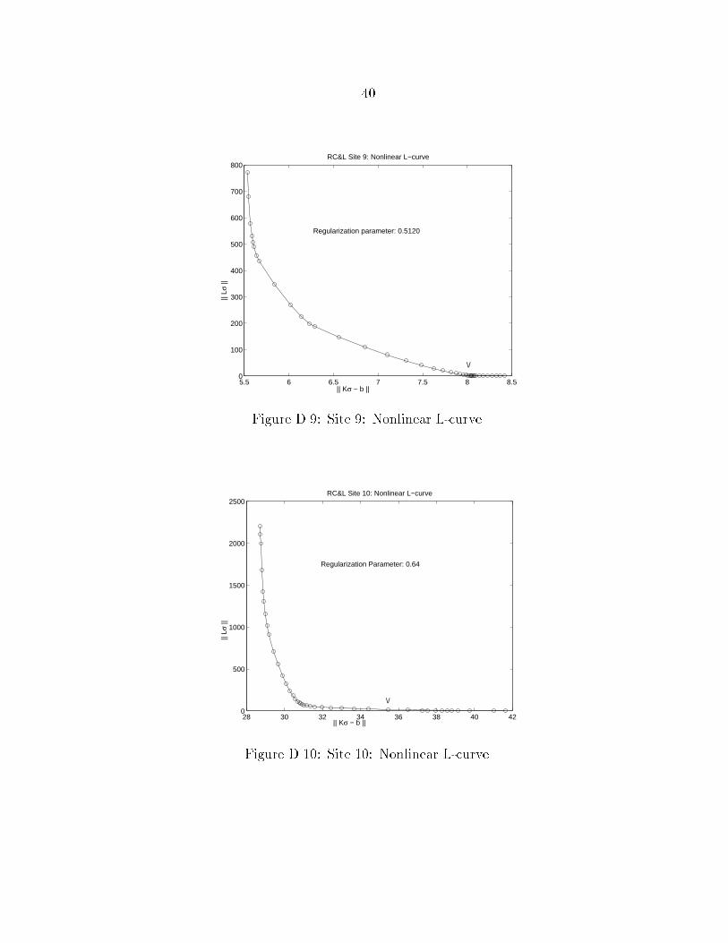
��
5.5 6 6.5 7 7.5 8 8.50
100
200
300
400
500
600
700
800RC&L Site 9: Nonlinear L−curve
|| Kσ − b ||
|| Lσ
||
\/
Regularization parameter: 0.5120
Figure D��� Site �� Nonlinear Lcurve�
28 30 32 34 36 38 40 420
500
1000
1500
2000
2500RC&L Site 10: Nonlinear L−curve
|| Kσ − b ||
|| Lσ
||
Regularization Parameter: 0.64
\/
Figure D���� Site ��� Nonlinear Lcurve�
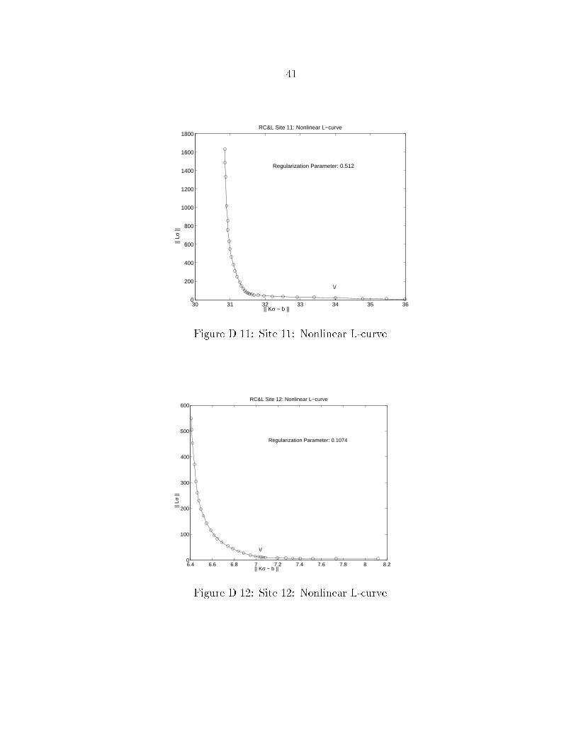
��
30 31 32 33 34 35 360
200
400
600
800
1000
1200
1400
1600
1800RC&L Site 11: Nonlinear L−curve
|| Kσ − b ||
|| Lσ
||
Regularization Parameter: 0.512
\/
Figure D���� Site ��� Nonlinear Lcurve�
6.4 6.6 6.8 7 7.2 7.4 7.6 7.8 8 8.20
100
200
300
400
500
600RC&L Site 12: Nonlinear L−curve
|| Kσ − b ||
|| Lσ
||
Regularization Parameter: 0.1074
\/
Figure D���� Site ��� Nonlinear Lcurve�
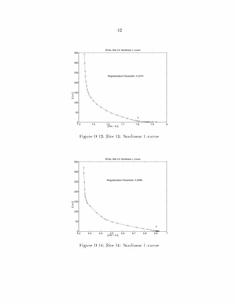
��
7.4 7.5 7.6 7.7 7.8 7.9 80
50
100
150
200
250
300
350RC&L Site 13: Nonlinear L−curve
|| Kσ − b ||
|| Lσ
||
\/
Regularization Parameter: 0.1074
Figure D���� Site ��� Nonlinear Lcurve�
6.2 6.3 6.4 6.5 6.6 6.7 6.8 6.9 70
50
100
150
200
250
300
350RC&L Site 14: Nonlinear L−curve
|| Kσ − b ||
|| Lσ
||
Regularization Parameter: 0.4096
\/
Figure D���� Site ��� Nonlinear Lcurve�
References
�Alumbaugh and Newman� ����� Alumbaugh� D� L� and Newman� G� A�
������� Threedimensional massively parallel electromagnetic inversion II�
analysis of a crosswell electromagnetic experiment� Geophysics� �������
����
�Alumbaugh et al�� ����� Alumbaugh� D� L�� Newman� G� A�� Prevost� L�� and
Shadid� J� N� ������� Threedimensional wideband electromagnetic modeling
on massively parallel computers� Radio Science� ���� ���
�Anderson� ����� Anderson� W� L� ������� Computer program numerical inte
gration of related Hankel transforms of orders � and � by adaptive digital
�ltering� Geophysics� ���������� �����
�Borchers et al�� ����� Borchers� B�� Uram� T�� and Hendrickx� J� M� �������
Tikhonov regularization of electrical conductivity depth pro�les in �eld soils�
Soil Science Society of America Journal� ���������� �����
�Engl� ����� Engl� H� W� ������� Regularization methods for the stable solu
tion of inverse problems� Surveys on Mathematics for Industry� ���� ����
�Forsythe et al�� ����� Forsythe� G� E�� Malcom� M� A�� and Moler� C� B�
������� Computer methods for mathematical computations� PrenticeHall�
Englewood Clis� New Jersey�
��
�Groetsch� ����� Groetsch� C� W� ������� Inverse Problems in the Mathemat�
ical Sciences� Vieweg� Bruanschweig! Wiesbaden�
�Hanke and Hansen� ����� Hanke� M� and Hansen� P� C� ������� Regulariza
tion methods for largescale problems� Surveys on Mathematics for Industry�
����� ����
�Hansen� ����� Hansen� P� C� ������� Numerical tools for analysis and solution
of Fredholm integral equations of the �rst kind� Inverse Problems� ����� ����
�Lawson and Hanson� ����� Lawson� C� L� and Hanson� R� J� ������� Solving
Least Squares Problems� PrenticeHall� Englewood Clis� New Jersey�
�McNeill� ����� McNeill� J� D� ������� Electromagnetic terrain conductivity
measurement at low induction numbers� Technical Report TN�� Geonics
Limited�
�McNeill� ����� McNeill� J� D� ������� EM�� � measurements at two intercoil
spacings to reduce sensitivity to near surface material� Technical Report
TN��� Geonics Limited�
�McNeill� ����� McNeill� J� D� ������� Use of electromagnetic methods for
groundwater studies� In Ward� S� H�� editor�Geotechnical and Environmental
Geophysics� volume �� pages ��� ���� Society of Exploration Geophysicists�
�Nabighian� ����� Nabighian� M� N�� editor ������� Electromagnetic Meth�
ods in Applied Geophysics� volume �� Society of Exploration Geophysicists�
Tulsa�
��

�Newman and Alumbaugh� ����� Newman� G� A� and Alumbaugh� D� L�
������� Threedimensional massively parallel electromagnetic inversion I�
Theory� Geophysics� ������� ����
�Parker� ����� Parker ������� Geophysical Inverse Theory� Princeton Univer
sity Press�
�Rhoades et al�� ����� Rhoades� J�� Corwin� D�� and Lesch� S� ������� Eect of
soil ECa depth pro�le pattern on electromagnetic induction measurements�
Technical Report ���� US Dept� of Agriculture Agricultural Research Ser
vice US Salinity Laboratory�
�Rhoades� ����� Rhoades� J� D� ������� Electrical conductivity methods for
measuring and mapping soil salinity� In Sparks� D� L�� editor� Advances In
Agronomy� volume � � pages ��� ���� Academic Press�
�Twomey� ����� Twomey� S� ������� Introduction to the Mathematics of In�
version in Remote Sensing and Indirect Measurements� Dover Publications�
Inc�� Mineola� New York�
�Wahba� ����� Wahba� G� ������� Spline Models for Observational Data�
SIAM� Philadelpqhia�
�Wait� ����� Wait� J� R� ������� Geo�Electromagnetism� Academic Press� New
York�
�Wing� ����� Wing� G� M� ������� A Primer on Integeral Equations of the
First Kind� SIAM� Philadelphia�
��

�Zauderer� ����� Zauderer� E� ������� Partial Di�erential Equations of Applied
Mathematics� John Wiley " Sons� Inc�� New York�
��

This thesis is accepted on behalf of the faculty of the Institute by the following
committee�
Advisor
Date


![A Nonlinear Dynamic Inversion Predictor-Based Model Reference Adaptive ...€¦ · dynamic inversion controller based in large part on [1], [2], and [3]. This control architecture](https://img.pdfslide.us/doc/110x75/5f0e40247e708231d43e55ae/a-nonlinear-dynamic-inversion-predictor-based-model-reference-adaptive-dynamic.jpg)