Linear and nonlinear Granger causality in the stock

price-volume relation: A perspective on the agent-based

model of stock markets

Shu-Heng ChenAI-ECON Research CenterDepartment of Economics

National Chengchi UniversityTaipei, Taiwan 116

E-mail: chchen@nccu.edu.tw

Chung-Chih LiaoGraduate Institute of International Business

National Taiwan UniversityTaipei, Taiwan 106

E-mail: ccliao@aiecon.org

Abstract

From the perspective of the agent-based model of stock markets, this paper ex-amines the possible explanations for the presence of the causal relation between stockreturns and trading volume. The implication of this result is that the presence ofthe stock price-volume causal relation does not require any explicit assumptions likeinformation asymmetry, reaction asymmetry, noise traders, or tax motives. In fact, itsuggests that the causal relation may be a generic property in a market modeled asevolving decentralized system of autonomous interacting agents.

Keyword: Agent-based model, Artificial stock markets, Genetic programming, Grangercausality test, Stock price-volume relation

1 Motivation and introduction

Agent-based modeling of stock markets, originated in Santa Fe Institute [44, 2], is a fer-tile and promising field, which can be thought as a subfield of agent-based computationaleconomics (ACE).1 Up to the present, most of the research efforts have been devoted tothe analysis of the price dynamics and/or market efficiency of the artificial markets (e.g.[13, 14, 41, 52]). Some focused their study on the price deviation or mispricing in theartificial stock markets (e.g. [2, 8, 10, 12, 40, 41, 44, 51]). Some of them went further toexplore the corresponding microstructure of the markets, such as aspect traders’ beliefs andbehaviors (e.g. [11, 13, 14]). Nevertheless, few have ever visited the univariate dynamicsof trading volume series [40, 51], and, to our best knowledge, none has addressed its jointdynamics with prices.2

1As Farmer and Lo [22] mentioned, “Evolutionary and ecological models of financial markets is trulya new frontier whose exploration has just begun.” By modeling financial markets “as evolving systemsof autonomous interacting agents,” the agent-based approach in finance, indeed, follows this evolutionaryparadigm [49]. Visit the ACE website maintained by Leigh Tesfatsion for a comprehensive guide to the fieldof agent-based computational economics. <URL: http://www.econ.iastate.edu/tesfatsi/ace.htm>

2See Chen [9] or LeBaron [39] for reviews of the field of artificial financial markets.

1

As Ying [53] noted almost forty years ago, stock prices and trading volume are jointproducts from one single market mechanism. He argued that “any model of the stockmarket which separates prices from volume or vice versa will inevitably yield incomplete ifnot erroneous results” [ibid., p. 676]. In similar vein, Gallant et al. [24] also asserted thatresearchers can learn more about the very nature of stock markets by studying the jointdynamics of prices in conjunction with volume, instead of focusing price dynamics alone.As a result, the stock price-volume relation has been an interesting subject in financialeconomics for many years.3

While most of the earlier empirical work focused on the contemporaneous relation be-tween trading volume and stock returns, some recent studies began to address the dy-namic relation, i.e., causality, between daily stock returns and trading volume followingthe notion of Granger causality proposed by Wiener [50] and Granger [26]. In manycases, a bi-directional Granger causality (or a feedback relation) was found to exist in thestock price-volume relation, although some other works could only find evidence of a uni-directional causality: either returns would Granger-cause trading volume, or vice versa[1, 34, 45, 46, 48].

As noted by Granger [27], Hsieh [33], and many others, we live in a world whichis “almost certainly nonlinear.” We can not be satisfied with only exploring the linearCausality between stock prices and trading volume. Non-linear causality would naturallybe the next step to pursue. Baek and Brock [3] argued that traditional Granger causalitytests based on VAR models might overlook significant nonlinear relations. As a result,they proposed a nonlinear Granger causality test by using nonparametric estimators oftemporal relations within and across time series. This approach can be applied to anytwo stationary, mutually independent and individually i.i.d. series. Hiemstra and Jones[31] modified their test slightly to allow the two series under considerations to display“weak (or short-term) temporal dependence.” Several researchers have already adoptedthis modified Baek and Brock test to uncover price and volume causal relation in realworld financial markets [23, 31, 47]. In most of the cases, they could found bi-directionalnonlinear Granger causality in the prices and trading volume. In other words, not onlydid stock returns Granger-cause trading volume, but trading volume also Granger-causestock returns. The significance of this finding is that trading volume can help predictstock returns, as an old Wall Street adage goes, “It takes volume to make price move.”

There are several possible explanations for the presence of a causal relation betweenstock returns and trading volume in the literatures. First, Epps [20] gave their explanationbased on the asymmetric reaction of two groups of investors — “bulls” and “bears” — tothe positive information and negative information.

The second explanation, which is called the mixture of distributions hypothesis, consid-ers special distributions of speculative prices. For example, Epps and Epps [21] derived amodel in which trading volume is used to measure disagreement of traders’ beliefs on thevariance of the price changes. On the other hand, in Clark’s [16] mixture of distributionsmodel, the speed of information flow is a latent common factor which influences stockreturns and trading volume simultaneously.

A third explanation is the sequential arrival of information models (see, for example,Copeland [17], He and Wang [30], Jennings et al. [35], and Morse [43]). In this asym-

3See the survey article by Karpoff [37].

2

metric information world, traders possess differential pieces of new information in thebeginning. Before the final complete information equilibrium is achieved, the informationis disseminated to different traders only gradually and sequentially. This implies a positiverelationship between price changes and trading volume.

Lakonishok and Smidt [38] proposed still another model which involves tax- and non-tax-related motives for trading. For the sake of window dressing, portfolio rebalancing,or the optimal timing for capital gains, traders may have some special kinds of tradingbehaviors. As a result, Lakonishok and Smidt [38] showed that current trading volumecan be related to past price changes owing to these motives.

Away from traditional representative-agent models stated above, recent theoreticalworks have started to model financial markets with heterogeneous traders. Besides in-formed traders (insiders), DeLong et al. [18] introduced noise traders with positive-feedback trading strategies in their model. Noise traders do not have any informationabout the fundamentals and trade solely based on the past price movements. As a result,positive causal relation from stock returns to trading volume appears. In Brock’s [5] non-linear theoretical noise trading model, the estimation errors made by different groups oftraders are correlated. Under these settings, he could find that stock price movements andvolatilities are related nonlinearly to volume movements. Campbell et al. [6] developedanother heterogenous agent model, in which there are two different types of risk-aversetraders. In their frameworks, they could explain the autocorrelation properties of stockreturns as a nonlinear relation with trading volume.

In light of these explanations, this paper attempts to see whether we can replicate thecausal relation between stock returns and the trading volume via the agent-based stock mar-kets (ABSMs). We consider the agent-based model of stock markets highly relevant tothis issue. First, the existing explanations mentioned above based their assumptions eitheron the information dissemination schemes or the traders’ reaction styles to informationarrival. Since both of these factors are well encapsulated in agent-based stock markets, itis interesting to see whether ABSMs are able to replicate the casual relation. Secondly,information dissemination schemes and traders’ behavior are known as the emergent phe-nomena in ABSMs. In other words, these factors are endogenously generated rather thanexogenously imposed. This feature can allows us to search for a fundamental explanationfor the causal relation. For example, we can ask: without the assumption of informationasymmetry, reaction asymmetry, or noise traders, and so on, can we still have the causalrelation? Briefly, is the causal relation a generic phenomenon?

Thirdly, we claim that agent-based modeling of financial markets are “true” heteroge-neous agent models, which depict the real markets more faithfully. We might think thatthe models proposed by DeLong et al. [18] and their successors as having pre-specifiedrepresentative agents of two different types, say, a representative rational informed traderand a representative uninformed noise trader. These settings might overlook some im-portant features of financial markets, for example, interaction and feedback dynamics oftraders. In the agent-based approach, we, however, do not assign any agent to be anyspecific type exogenously. As a matter of fact, we don’t even have the device of repre-sentative agents. Hundreds of agents in the model can all have different behavioral ruleswhich themselves shall evolve (adapt) over time.4 How many types by which they can be

4This model of agents follows the notion mentioned by Lucas [42, p. S401], “. . . we view or modelan individual as a collection of decision rules. . . . These decision rules are continuously under review

3

distinguished and what these types should be are difficult issues to be addressed withinthis highly dynamical evolving environment.

Finally, in agent-based stock markets, we can also observe what agents (artificialtraders) really believe in the deep of their mind when they are trading. This explo-ration is probably the most striking feature of the agent-based social simulation paradigm.Not only can we observe the macro-phenomena of our artificial society, e.g. the jointdynamics of prices and trading volume; but we can also watch the micro-behavior of ev-ery heterogeneous agents to the details of their thought processes, e.g. the forecastingmodels or trading strategies these agents used. Via this feature, we can then trace howthe behaviors and interaction of agents in the mirco-level could generate the macro-levelphenomena. Furthermore, we may see whether the agents’ watching macro-phenomenawould change their behaviors, and hence may transform the whole financial dynamics intodifferent scenarios (the so-called regime change). These complex feedback relations cannot be well captured by the traditional representative agent model.

The rest of the paper is organized as follows. Section 2 describes the agent-based stockmarket considered in this paper. In Section 3, we briefly depicts experimental designs weadopted. Section 4 introduces the concept of Granger causality and two different econo-metric test used in this paper. Section 5 gives the simulation and testing results both ofthe “top” and of the “bottom”, followed by the concluding remarks in Section 6.

2 The agent-based artificial stock market

The agent-based stock markets considered in this paper is AIE-ASM, version 3, developedby AI-ECON Research Center [13, 15]. The basic framework of the AIE-ASM is thestandard asset pricing model in the vein of Grossman and Stiglitz [28]. The dynamics ofthe market is determined by interactions of many heterogeneous agents. Each of them,based on his forecast of the future, maximizes his expected utility.

2.1 Traders

For simplicity, we assume that all traders share the same constant absolute risk aversion(CARA) utility function,

U(Wi,t) = − exp(−λWi,t), (1)

where Wi,t is the wealth of trader i at period t, and λ is the degree of absolute risk aversion.Traders can accumulate their wealth by making investments. There are two assets availablefor traders to invest. One is the riskless interest-bearing asset called money, and the otheris the risky asset known as the stock. In other words, at each period, each trader has twoways to keep his wealth, i.e.,

Wi,t = Mi,t + Pthi,t, (2)

where Mi,t and hi,t denote the money and shares of the stock held by trader i at period trespectively, and Pt is the price of the stock at period t. Given this portfolio (Mi,t,hi,t), a

and revision; new decision rules are tried and tested against experience, and rules that produce desirableoutcomes supplant those that do not.” (Italics added.) To model this kind of adapting agents, agent-basedcomputational economists borrow multi-agent techniques and artificial intelligence (AI) tools from the fieldof computer science.

4

trader’s total wealth Wi,t+1 is thus

Wi,t+1 = (1 + r)Mi,t + hi,t(Pt+1 + Dt+1), (3)

where Dt is per-share cash dividends paid by the companies issuing the stocks and r isthe riskless interest rate. Dt can follow a stochastic process not known to traders. Giventhis wealth dynamics, the goal of each trader is to myopically maximize the one-periodexpected utility function,

Ei,t

(U(Wi,t+1)

)= E

(− exp(−λWi,t+1)

∣∣Ii,t

), (4)

subject to Equation (3), where Ei,t(·) is trader i’s conditional expectations of Wt+1 givenhis information up to t (the information set Ii,t).

It is well known that under CARA utility and Gaussian distribution for forecasts, traderi’s desire demand, h∗

i,t+1 for holding shares of risky asset is linear in the expected excessreturn:

h∗i,t =

Ei,t(Pt+1 + Dt+1)− (1 + r)Pt

λσ2i,t

, (5)

where σ2i,t is the conditional variance of (Pt+1 + Dt+1) given Ii,t.

The key point in the agent-based artificial stock market is the formation of Ei,t(·). Inthis paper, the expectation is modeled by genetic programming. The detail is described inthe next subsection.

2.2 Price Determination

Given h∗i,t, the market mechanism is described as follows. Let bi,t be the number of shares

trader i would like to submit a bid to buy at period t, and let oi,t be the number of sharestrader i would like to offer to sell at period t. It is clear that

bi,t ={

h∗i,t − hi,t−1, h∗

i,t ≥ hi,t−1,

0, otherwise,(6)

and

oi,t ={

hi,t−1 − h∗i,t, h∗

i,t < hi,t−1,

0, otherwise.(7)

Furthermore, let

Bt =N∑

i=1

bi,t, and Ot =N∑

i=1

oi,t

be the totals of the bids and offers for the stock at period t, where N is the number oftraders. Following Palmer et al. [44], we use the following simple rationing scheme:

hi,t =

hi,t−1 + bi,t − oi,t, if Bt = Ot,

hi,t−1 +Ot

Btbi,t − oi,t, if Bt > Ot,

hi,t−1 + bi,t −Bt

Otoi,t, if Bt < Ot.

(8)

5

All these cases can be subsumed into

hi,t = hi,t−1 +Vt

Btbi,t −

Vt

Otoi,t, (9)

where Vt ≡ min(Bt, Ot) is the volume of trade in the stock.According to Palmer et al.’s rationing scheme, we can have a very simple price adjust-

ment scheme, based solely on the excess demand Bt −Ot:

Pt+1 = Pt

(1 + β(Bt −Ot)

)(10)

where β is a function of the difference between Bt and Ot. β can be interpreted as thespeed of adjustment of prices. The β function we consider is:

β(Bt −Ot) ={

tanh(β1(Bt −Ot)

), if Bt ≥ Ot,

tanh(β2(Bt −Ot)

), if Bt < Ot,

(11)

where tanh is the hyperbolic tangent function:

tanh(x) ≡ ex − e−x

ex + e−x.

The price adjustment process introduced above implicitly assumes that the total num-ber of shares of the stock circulated in the market is fixed, i.e.,

Ht =N∑

i=1

hi,t = H. (12)

In addition, we assume that dividends and interests are all paid by cash, so

Mt+1 =N∑

i=1

Mi,t+1 = Mt(1 + r) + HtDt+1. (13)

2.3 Formation of Expectations

As to the formation of traders’ expectations, Ei,t(Pt+1 + Dt+1), we assume the followingfunctional form for Ei,t(·).5

Ei,t(Pt+1 + Dt+1) =

(Pt + Dt)(1 + θ1fi,t × 10−4), if − 104 ≤ fi,t ≤ 104,(Pt + Dt)(1 + θ1), if fi,t > 104,(Pt + Dt)(1− θ1), if fi,t < −104.

(14)

The population of fi,t (i=1,. . . ,N) is formed by genetic programming. That means, thevalue of fi,t is decoded from its GP tree gpi,t.6

As to the subjective risk equation, we modified the equation originally used by Arthuret al. [2],

σ2i,t = (1− θ2)σ2

t−1|n1+ θ2

(Pt + Dt − Ei,t−1(Pt + Dt)

)2, (15)

5There are several alternatives to model traders’ expectations. The interested reader is referred to Chenet al. [15].

6See Chen and Yeh [13] for more details about the GP-based evolutionary forecasting processes.

6

where

σ2t−1|n1

=

∑n1−1j=0 (Pt−j − P t|n1

)2

n1 − 1,

and

P t|n1=

∑n1−1j=0 Pt−j

n1.

In other words, σ2t−1|n1

is simply the historical volatility based on the past n1 observations.Given each trader’ expectations, Ei,t(Pt+1 + Dt+1), according to equation (5) and his

own subjective risk equation, we can obtain each trader’s desire demand, h∗i,t+1 shares of

the stock, and then how many shares of stock each trader intends to bid or offer based onequation (6) or (7).

3 Experimental designs and data description

3.1 Experimental designs

As mentioned earlier, our simulations are based on the software, AIE-ASM, version 3. Atutorial on this software can be found in Chen et al. [15]. This tutorial would help explainmost of the parameters shown in Table 1 and 2, which we shall skip its details exceptmentioning that most parameter values are taken from Chen and Yeh [13]. The simulationspresented in this paper are mainly based on three different designs. These designs aremotivated by our earlier studies on the ABSM, in particular, Chen and Yeh [13, 14] andChen and Liao [10]. These three designs differs in two key economic parameters, namely,dividend processes and risk attitude.

In Market A, the baseline market, the dividend process is assumed to be iid Gaussiandistribution and the traders’ measure of absolute risk aversion (λ) are assumed to be 0.1.In Market B, the traders are assumed to be more risk-averse, which is characterized bya higher degree of absolute risk aversion (λ = 0.5). As to Market C, the dividends areassumed to be iid uniform distribution, while the traders’ attitude toward risk are assumedto be the same as that of the baseline market. Three runs each with 5000 generationswas conducted for each of the three markets. Table 2 is a summary of our experimentaldesigns.

3.2 Data description

The data generated from each run of simulation is then used to test the existence of price-volume relation. As we mentioned in Section 1, Granger causality is used to define thedynamic relation between prices and trading volume. Following the standard econometricprocedure, we first applied the augmented Dickey-Fuller unit root test to examine thestationarities of the price series, Pt, and trading volume series, Vt. Based on the testingresults, difference transformation was taken to make sure that all time series are stationary:

rt = ln(Pt)− ln(Pt−1), vt = Vt − Vt−1,7

7The reason that we did not take the log-difference transformation for volume is that trading volumemay be zero in some trading periods.

7

Table 1: Parameters of the stock marketThe Stock Market

Share per capita (h) 1Initial money supply per capita (m) 100Interest Rate (r) 0.1Stochastic process (Dt) i.i.d. Normal(µ = 10, σ2 = 4)

[Market A, Market B]i.i.d. Uniform(5,15) [Market C]

Price adjustment function tanhPrice adjustment (β1) 10−4

Price adjustment (β2) 0.2× 10−4

Traders

Number of traders 500Degree of ARA (λ) 0.1 [Market A, Market C], 0.5 [Market B]Criterion of fitness (traders) Increments in wealthSample size of σ2

t 10Evaluation cycle 1Sample size 10Search intensity 5θ1 0.5θ2 10−4

θ3 0.0133

where rt is also known as stock return. We then examined the causal relation betweenrt and vt. To test whether there is any uni-directional causality from one variable to theother, we followed the conventional approach in econometrics, i.e. linear Granger causalitytest and, for nonlinear case, the modified Baek and Brock test. There are several differ-ent ways to conduct the Granger causality test: some tests require an arbitrary choice offiltering processes, and others require an arbitrary choice of lags. We shall briefly presentthese notions of causality and the procedures of tests in the next section.

4 Wiener-Granger causality: definition and testing

The concept of causality plays a crucial role in many empirical economic studies, andis particularly important for our understanding and interpretation of dynamic economicphenomena. Nevertheless, it is difficult to give a formal notion of causality. This issue,in fact, is a philosophical one (see, e.g. Geweke [25]). Wiener [50], however, proposed awidely accepted concept of causality based on predictive relation between the two timeseries in question. This notion of causality, known as Wiener-Granger causality (or simplyGranger causlaity), was then introduced to economists by Granger [26].

In this section, we first review the definition of causality in Wiener-Granger’s sense, fol-lowed by introducing two different versions of Granger-causality tests proposed by Granger

8

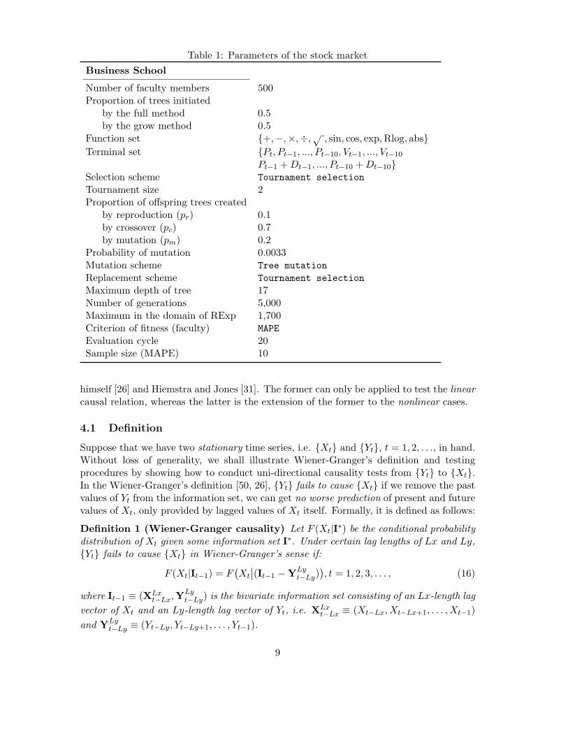
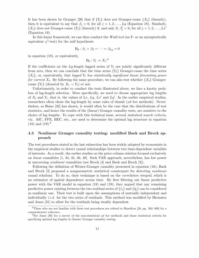
Table 1: Parameters of the stock marketBusiness School

Number of faculty members 500Proportion of trees initiated

by the full method 0.5by the grow method 0.5

Function set {+,−,×,÷,√

, sin, cos, exp,Rlog, abs}Terminal set {Pt, Pt−1, ..., Pt−10, Vt−1, ..., Vt−10

Pt−1 + Dt−1, ..., Pt−10 + Dt−10}Selection scheme Tournament selectionTournament size 2Proportion of offspring trees created

by reproduction (pr) 0.1by crossover (pc) 0.7by mutation (pm) 0.2

Probability of mutation 0.0033Mutation scheme Tree mutationReplacement scheme Tournament selectionMaximum depth of tree 17Number of generations 5,000Maximum in the domain of RExp 1,700Criterion of fitness (faculty) MAPEEvaluation cycle 20Sample size (MAPE) 10

himself [26] and Hiemstra and Jones [31]. The former can only be applied to test the linearcausal relation, whereas the latter is the extension of the former to the nonlinear cases.

4.1 Definition

Suppose that we have two stationary time series, i.e. {Xt} and {Yt}, t = 1, 2, . . ., in hand.Without loss of generality, we shall illustrate Wiener-Granger’s definition and testingprocedures by showing how to conduct uni-directional causality tests from {Yt} to {Xt}.In the Wiener-Granger’s definition [50, 26], {Yt} fails to cause {Xt} if we remove the pastvalues of Yt from the information set, we can get no worse prediction of present and futurevalues of Xt, only provided by lagged values of Xt itself. Formally, it is defined as follows:

Definition 1 (Wiener-Granger causality) Let F (Xt|I∗) be the conditional probabilitydistribution of Xt given some information set I∗. Under certain lag lengths of Lx and Ly,{Yt} fails to cause {Xt} in Wiener-Granger’s sense if:

F (Xt|It−1) = F(Xt

∣∣(It−1 −YLyt−Ly)

), t = 1, 2, 3, . . . , (16)

where It−1 ≡ (XLxt−Lx,YLy

t−Ly) is the bivariate information set consisting of an Lx-length lagvector of Xt and an Ly-length lag vector of Yt, i.e. XLx

t−Lx ≡ (Xt−Lx, Xt−Lx+1, . . . , Xt−1)and YLy

t−Ly ≡ (Yt−Ly, Yt−Ly+1, . . . , Yt−1).

9

Table 2: Experimental Designs

Market Case Stochastic Process of Dividends Measure of ARA‡

Market A A1, A2, A3 i.i.d. Normal(µ = 10, σ2 = 4) 0.1Market B B1, B2, B3 i.i.d. Normal(µ = 10, σ2 = 4) 0.5Market C C1, C2, C3 i.i.d. Uniform(5,15) 0.1

‡ Note that ARA stands for absolute risk aversion.

Conversely, if the lagged values of Yt have predictive power for the present and futurevalues of Xt, then we conclude that the time series {Yt} Wienr-Granger-cause (or simplyGranger-cause) the time series {Xt}.

4.2 Linear Granger causality testing: vector autoregression (VAR) ap-proach

Based on the definition given above, Wiener-Granger causality refers to a historical pathof one time series which influences the probability distribution of the present and futurepath of another time series. However, the definition in equation (16) is not easy to test.Granger [26], therefore, proposed a testable form by restricting the original concept toa linear prediction model. In other words, he assumed that predictors are least-squaresprojections, and mean square error (MSE) is adopted to be the criterion for comparingpredictive power:

Definition 2 (linear Granger causality) Given certain lag lengths of Lx and Ly, {Yt}fails to linearly Granger-cause {Xt} (denoted by Yt 9 Xt) if:

MSE(E(Xt|It−1)

)= MSE

(E(Xt|(It−1 −YLy

t−Ly)), (17)

where MSE(E(Xt|I∗)

)denotes the mean square error for a prediction of Xt based on some

information set I∗.

According to the definition of (linear) Granger causality given above, we now consider thefollowing well-known bivariate vector autoregression (VAR) equations:

Xt = c +Lx∑i=1

αiXt−i +Ly∑j=1

βjYt−j + εt, (18)

Yt = c′ +Ly′∑i=1

α′iYt−i +

Lx′∑j=1

β′jXt−j + ηt, (19)

where the disturbances, {εt} and {ηt}, are two uncorrelated series following the conven-tional assumptions of white noises, say, they are i.i.d. with zero mean and some commonvariance of σ2 such that

E(εtεs) = E(ηtηs) = 0, ∀ s 6= t,

andE(εtηs) = 0, ∀ s, t.

10

It has been shown by Granger [26] that if {Yt} does not Granger-cause {Xt} (linearly),then it is equivalent to say that βj = 0, for all j = 1, 2, . . . , Ly (Equation 18). Similarly,{Xt} does not Granger-cause {Yt} (linearly) if, and only if, β′

j = 0, for all j = 1, 2, . . . , Lx′

(Equation 19).In this linear framework, we can then conduct the Wald test (an F- or an asymptotically

equivalent χ2-test) for the null hypothesis:

H0 : β1 = β2 = · · · = βLy = 0

in equation (18), or equivalently,H0 : Yt 9 Xt.

8

If the coefficients on the Ly-length lagged series of Yt are jointly significantly differentfrom zero, then we can conclude that the time series {Yt} Granger-cause the time series{Xt}, or, equivalently, that lagged Yt has statistically significant linear forecasting powerfor current Xt. By following the same procedure, we can also test whether {Xt} Granger-cause {Yt} (denoted by Xt → Yt) or not.

Unfortunately, in order to conduct the tests illustrated above, we face a knotty prob-lem of lag-length selection. More specifically, we need to choose appropriate lag lengthsof Xt and Yt, that is, the values of Lx, Ly, Lx′ and Ly′. In the earlier empirical studies,researchers often chose the lag-length by some rules of thumb (ad hoc methods). Never-theless, as Hsiao [32] has shown, it would often be the case that the distributions of teststatistics, and hence the results of the (linear) Granger causality tests, are sensitive to thechoice of lag lengths. To cope with this technical issue, several statistical search criteria,viz. AIC, FPE, BEC, etc., are used to determine the optimal lag structure in equation(18) and (19).9

4.3 Nonlinear Granger causality testing: modified Baek and Brock ap-proach

The test procedures stated in the last subsection has been widely adopted by economists inthe empirical studies to detect causal relationships between two time-dependent variablesof interests. As a result, the earlier studies on the price-volume relation focused exclusivelyon linear causalities [1, 34, 45, 46, 48]. Such VAR approach, nevertheless, has low powerin uncovering nonlinear causalities (see Brock [4] and Baek and Brock [3]).

Following the definition of Weiner-Granger causality presented in equation (16), Baekand Brock [3] proposed a nonparametric statistical counterpart for detecting nonlinearcausal relations. To do so, their technique is based on the correlation integral, which isan estimator of spatial dependence across time. By first filtering out linear predictivepower with the VAR model in equation (18) and (19), they argued that any remainingpredictive power existing between the two residual series of {εt} and {ηt} can be consideredas nonlinear one. Their test is built upon the assumptions of mutually independent andindividually i.i.d. for the two series of residuals. This method was modified by Hiemstraand Jones [31] to allow for the residuals being weakly dependent.

8Those who are not familiar with these test procedures are refered to Hamilton [29, pp. 302–309] for acomprehensive reference.

9See Jones [36] for a survey of the non-statistical ad hoc methods and those statistical criteria forspecifying optimal lag lengths in (linear) Granger causality testing.

11

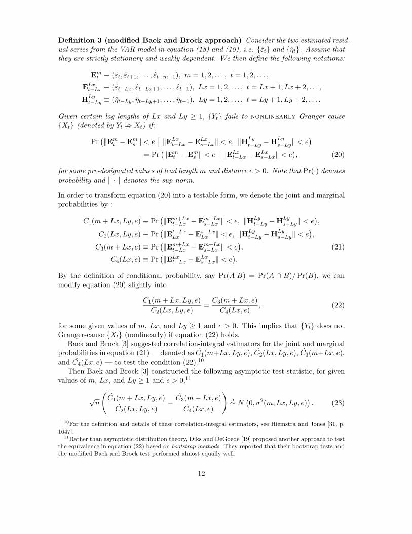
Definition 3 (modified Baek and Brock approach) Consider the two estimated resid-ual series from the VAR model in equation (18) and (19), i.e. {εt} and {ηt}. Assume thatthey are strictly stationary and weakly dependent. We then define the following notations:

Emt ≡ (εt, εt+1, . . . , εt+m−1), m = 1, 2, . . . , t = 1, 2, . . . ,

ELxt−Lx ≡ (εt−Lx, εt−Lx+1, . . . , εt−1), Lx = 1, 2, . . . , t = Lx + 1, Lx + 2, . . . ,

HLyt−Ly ≡ (ηt−Ly, ηt−Ly+1, . . . , ηt−1), Ly = 1, 2, . . . , t = Ly + 1, Ly + 2, . . . .

Given certain lag lengths of Lx and Ly ≥ 1, {Yt} fails to nonlinearly Granger-cause{Xt} (denoted by Yt ; Xt) if:

Pr(‖Em

t −Ems ‖ < e

∣∣ ‖ELxt−Lx −ELx

s−Lx‖ < e, ‖HLyt−Ly −HLy

s−Ly‖ < e)

= Pr(‖Em

t −Ems ‖ < e

∣∣ ‖ELxt−Lx −ELx

s−Lx‖ < e), (20)

for some pre-designated values of lead length m and distance e > 0. Note that Pr(·) denotesprobability and ‖ · ‖ denotes the sup norm.

In order to transform equation (20) into a testable form, we denote the joint and marginalprobabilities by :

C1(m + Lx, Ly, e) ≡ Pr(‖Em+Lx

t−Lx −Em+Lxs−Lx ‖ < e, ‖HLy

t−Ly −HLys−Ly‖ < e

),

C2(Lx, Ly, e) ≡ Pr(‖Et−Lx

Lx −Es−LxLx ‖ < e, ‖HLy

t−Ly −HLys−Ly‖ < e

),

C3(m + Lx, e) ≡ Pr(‖Em+Lx

t−Lx −Em+Lxs−Lx ‖ < e

), (21)

C4(Lx, e) ≡ Pr(‖ELx

t−Lx −ELxs−Lx‖ < e

).

By the definition of conditional probability, say Pr(A|B) = Pr(A ∩ B)/ Pr(B), we canmodify equation (20) slightly into

C1(m + Lx,Ly, e)C2(Lx, Ly, e)

=C3(m + Lx, e)

C4(Lx, e), (22)

for some given values of m, Lx, and Ly ≥ 1 and e > 0. This implies that {Yt} does notGranger-cause {Xt} (nonlinearly) if equation (22) holds.

Baek and Brock [3] suggested correlation-integral estimators for the joint and marginalprobabilities in equation (21) — denoted as C1(m+Lx, Ly, e), C2(Lx, Ly, e), C3(m+Lx, e),and C4(Lx, e) — to test the condition (22).10

Then Baek and Brock [3] constructed the following asymptotic test statistic, for givenvalues of m, Lx, and Ly ≥ 1 and e > 0,11

√n

(C1(m + Lx, Ly, e)

C2(Lx, Ly, e)− C3(m + Lx, e)

C4(Lx, e)

)a∼ N

(0, σ2(m,Lx,Ly, e)

). (23)

10For the definition and details of these correlation-integral estimators, see Hiemstra and Jones [31, p.1647].

11Rather than asymptotic distribution theory, Diks and DeGoede [19] proposed another approach to testthe equivalence in equation (22) based on bootstrap methods. They reported that their bootstrap tests andthe modified Baek and Brock test performed almost equally well.

12

The asymptotic Gaussian distribution of this test statistic holds under the null hypothesisthat {Yt} does not Granger-cause {Xt} (nonlinearly), i.e. H0 : Yt ; Xt. By furtherusing the delta method,12 Hiemstra and Jones [31, pp. 1660–1662] suggested a consistentestimator for σ2(m,Lx,Ly, e) in equation (23) to conduct the test emiprically.

Note that a significant positive value in equation (23) suggests that {Yt} does Granger-cause {Xt} (nonlinearly). Nevertheless, a significant negative test statistic represents that“knowledge of the lagged values of Y confounds the prediction of X” (italics added, seeHiemstra and Jones [31, p. 1648]). Thus, we conduct the modified Baek and Brock testwith right-tailed critical values. Like the VAR approach in linear Granger-causality testing,we face the difficulties in choosing appropriate lagged length of Lx and Ly. Unfortunately,unlike linear Granger-causality testing, there is no literature discussing how to specify theoptimal values of those parameters, i.e. m, Lx, Ly, and e. In this paper, we simply followHiemstra and Jones [31] to tackle this issue.

5 Experimental results

We first summarize some basic descriptive statistics of our simulation results in Table 3.13

Some essential features, such as price deviation (or price discovery) and excess volatility,were already studied in our earlier paper [10, 12]. The summary statistics reported in thistable shows nothing significantly different from what we already discussed. We, therefore,shall focus exclusively on the price-volume relation in this paper. The presentation of ourresults shall follow the sequence indicated below. First, we start from the aggregate data(the macro-level). At this level, the issue concerns us is whether price-volume causalityexists. Second, we then go down to the “bottom” level, and examine the microstructureof traders. Finally, what we have found at the “top” is compared to what we found at the“bottom”, to see whether the micro-macro relation can be consistent.

5.1 Aggregate outcomes: Granger causality at the “top”

Table 4 gives the testing result of linear causality. The result is mixing. In some cases,the causal relation is not found in both directions. In some other cases, the uni-directioncausality is found. Clearly, the existence of the causal relation is not definite. This pictureis somewhat in line with what we learned from the literature: some found the existenceof linear causality, while some didn’t.

Table 5 shows the result of nonlinear causality, and the result is also inconclusive, which12The delta method is a prevailing tool in econometric studies. It helps to derive asymptotic distributions

for arbitrary nonlinear functions of an estimator. See Cambpell et al. [7, p. 540] for a brief illustration.13Note that HREEP stands for homogeneous rational expectation equilibrium price. In the model which

we construct in section 2, it can be derived that

HREEP =1

r(d− λσ2

dH

N),

by further incorporating the assumptions of a representative-agent with rational expectation and perfectforesight. See Chen and Liao [10] for the proof. We further define P = 1

T

∑Pt, MAPE = 1

T

∑ ∣∣Pt−HREEPHREEP

∣∣,and MPE = 1

T

∑ (Pt−HREEP

HREEP

)to show how far the artificial stock prices deviate from the HREE price.

Also note that σP , the standard deviation of prices, shows the price volatility of the artificial stock markets.

13

Table 3: Basic Descriptive Statistics

Case HREEP P MAPE MPE σP

A1 96 104.72 9.21% 9.08% 5.004A2 96 103.84 8.39% 8.16% 5.085A3 96 104.54 9.07% 8.90% 5.054

B1 80 84.25 6.01% 5.31% 3.967B2 80 84.53 6.16% 5.66% 3.762B3 80 84.21 5.93% 5.26% 3.838

C1 91.667 108.32 18.16% 18.16% 5.350C2 91.667 108.24 18.08% 18.08% 5.359C3 91.667 108.54 18.42% 18.41% 5.666

is also consistent with what we experienced from the literature. The bi-directional non-linear causality is found only in case B2 and B3, while the uni-directional causality fromreturn to volume exists in many cases. The return-to-volume casual relation is in generalmuch stronger than the volume-to-return causality.

Table 4: Linear Granger causality test

H0 : Volume changes do not H0 : Stock returns do notcause stock returns (vt 9 rt) cause volume changes (rt 9 vt)

Case # of Lags F-value p-value # of Lags F-value p-value

A1 16 1.942 0.0134∗ 20 1.030 0.4218A2 7 1.154 0.3261 18 1.243 0.2166A3 16 1.398 0.1324 18 1.246 0.2145

B1 10 1.262 0.2459 20 1.020 0.4331B2 10 4.832 0.0000∗ 20 1.074 0.3701B3 10 2.510 0.0052∗ 18 1.314 0.1672

C1 7 0.579 0.7733 20 0.503 0.9671C2 14 0.650 0.8244 20 0.987 0.4744C3 8 2.519 0.0099∗ 17 0.897 0.5778

Note that a ∗ represents statistical siginifance at the 5% significance level, whereasa † represents statistical siginifance at the 10% significance level.

5.2 Traders’ behavior: Granger causality at the “bottom”

Coming down to the “bottom” of the ABSM, we are interested in knowing the belief ofagents. Did agents believe the price-volume relation? Did they actually apply volume totheir forecasts of prices (returns)? To answer these questions, we have to check how manytraders might in fact use past trading volume as useful information during forecasting

14

processes in the deep of their mind. That is to say, we have to check whether the tradersincorporated trading volume into their expectation-generating formula (their GP trees).

To make the discussion convenient, we shall call those who believe trading volume asuseful information to predict future prices as price-volume believers. Applying the tech-nique invented by Chen and Yeh [14], we counted the number of price-volume believers.Since the counting work is very computational demanding, a cencus was made only afterevery 500 generations. This number is given in Table 6. In some cases, say B3, C1, andC2, the belief of price-volume relation prevails in the public from the beginning even tothe end of the simulations. In some other cases, such as A1, A3, and C3, price-volumebelievers finally died out of the markets in the end. Note that the number of price-volumebelievers may fluctuate during the whole simulation periods, e.g. B1 and B2. A strikingphenomena is that price-volume believers may revive even after some periods of noughts.A2 is a case in point. We now ready to check whether the marco-phenomena of price-volume relation we observed at the “top” matches what we observed at the “bottom”.This issue, called consistency, is checked in the next subsection.

5.3 The macro-micro relation

In the agent-based modeling framework, we are particularly interested in the so-calledmacro-micro relation. Based on the simulation results we have, four basic patterns standout. They can be roughly divided into two categories, namely, consistent patterns and in-consistent ones. A pattern is called consistent if the macro behavior tends to lend supportto what most individuals believe or come to believe. A pattern is called inconsistent if themacro behavior tends to invalidate what most individual believe or come to believe (seeTable 7).

In a more technical way, let that the volume does not Granger-cause returns be the nullhypothesis. If this null hypothesis is rejected (or failed to reject) by the aggregate marketoutcome based on econometric tests, then we say the pattern is consistent if it is alsorejected (or failed to reject) by most or by an increasing number of market participants.Otherwise, it is called inconsistent.

According to the definition above, the case A2, A3, B1 and B3 exhibit consistent pat-terns (the main diagonal boxes on Table 7), whereas the case A1, B2, C1, C2 and C3demonstrate inconsistent patterns (on the off-diagonal boxes on Table 7).

Among the consistent patterns, B3 is the case that the null hypothesis is consistentlyrejected by both macro and micro behavior. Its number of price-volume believers is per-sistently high during the entire simulation. In particular, for the second half of the tradingsession, almost all agents rejected the null by forecasting returns with volume (see Table6).

A2, A3 and B1 are the other consistent patterns. In these three cases, the null wasfailed to reject in both linear and nonlinear tests, and our traders’ beliefs were in line withthis test result. The number of participants who believe the null hypothesis continuouslydecreased. For example, consider the case A3. At the beginning, there are a great numberof traders who used volume in their forecasts of returns. Nonetheless, after period 1500,the number dramatically drops down from 300 to 100, and further to nil.

Among the inconsistent patterns (patterns on the off-diagonal of Table 7), C1 and

15

C2 share the feature that the market is composed of hundreds of price-volume believers,while the causality test shows that the volume cannot help predict returns. This resultis particular striking for the case C2, where the market reached a state where all marketparticipants are price-volume believers.

Equally interesting inconsistent patters are cases A1, B2 and C3. In these cases, thecausality test did indicate the significance of volume in return forecasting, but traderseventually gave up the use of this variable in their forecasts of returns.

5.4 Discussions

The analysis so far is mainly driven by the aggregate outcome. Basically, we are askingwhether the individual behavior is consistent with our econometric tests. In other words,if our tests suggest the casual relation, did our “smart” and “adaptive” also notice so?

The real issue is whether those inconsistent patterns are unanticipated or puzzling us.The answer is no. There are, in effect, some arguments to predict why these inconsistentpatterns may appear. For example, consider the cases C1 and C2. A supportive argumentwould be following: it is the intensive search, characterized by a large number of price-volume believers, over the hidden relation between volume and returns eventually nullifythe effect of volume on returns and make volume be an useless variable. In this case, themicro and macro relation observed in cases A3 and B3 is actually also in harmony witheach other. As a matter of fact, using this argument, one can question whether thoseconsistent patterns are really consistent. For instance, if no one give the volume variablea try, would it possible that the volume-to-price relation can finally emerge, as a secretwhich has never been disclosed?

The argument which we have just been through points out one serious issue in ourabove-proposed analysis of micro and macro relation. In this analysis, we treat the wholemicro process as one sample, and the whole macro process as the other sample. We thenlook into the consistence between the two. However, what was neglected is the complexdynamic feedback relation existing between aggregate outcome and individual behavior.As well depicted by Farmer and Lo [22, p. 9992],

Patterns in the price tend to disappear as agents evolve profitable strategiesto exploit them, but this occurs only over an extended period of time, duringwhich substantial profits may be accumulated and new patterns may appear.

As to the cases A1 and C3, we saw that there exists only linear Granger causalitybetween returns and trading volume at the macro level. Nevertheless, from the microviewpoint, traders were not aware of this. One possible explanation for observing suchkind of inconsistency is the huge search space defined by GP. The set of linear function hasonly a measure of zero in it. If we restrict our attention only to the non-linear causalitytest, then there is no inconsistency for the cases A1 and C3. It follows that traders mayoverlook the usefulness of linear models, and spent most of their trials over the space ofnon-linear models. As we may expect, they eventually gave up their attempts, becausenon-linear causality does not exist. However, this explanation can not applied to Case B2,in which nonlinear-causal relation is also shown to exist statistically significantly.

16

To sum up, there is no definite relation between micro and macro behavior. The ap-pearance of the patterns on the off-diagonal entries shows that the Neo-classical economicanalysis, which generally assumes the consistency between the micro and macro behavior,does not have a solid ground. It is in this agent-based economic model we show how easilyone can have aggregate result which is not anticipated from the individual behavior. Thereason that one can have such a large variety of patterns is mainly because of complexdynamic interaction between individuals and the market.

Financial market dynamics is path-dependent, highly complex and nonlinear because itis the outcome of continuously evolving and interacting behavior, which is mainly drivenby survival pressure. It is therefore difficult to make a simple conclusion on the relationbetween micro and macro behavior. To fully trace their interaction, the analysis based onhigh-frequency sampling (or census) of traders’ behavior is required. Statistical analysisbased on small samples is also useful to investigate the potential time variant relation, dueto the real time survival pressure.

6 Conclusions

One distinguishing feature of ACE (and thus ABSMs) is that some interesting macro phe-nomena of financial markets could emerge (be endogenously generate) from interactionsof adaptive agents without exogenously imposing any conditions like unexpected events,information cascade, noise or dumb traders, etc. In this paper, we show that the presenceof the stock price-volume causal relation does not require any explicit assumptions likeinformation asymmetry, reaction asymmetry, noise traders, or tax motives. In fact, itsuggests that the causal relation may be a generic property in a market modeled as anevolving decentralized system of autonomous interacting agents.

We also show that our understanding of the appearance or disappearance of the price-volume relation can never be complete if the feedback relation between individual behaviorand aggregate outcome is neglected. This feedback relation is, however, highly complex,which may defy any simple analysis, as the one we proposed initially. Consequently, econo-metric analysis which fails to take into account this complex feedback relation betweenmicro and macro may produce misleading results. Unfortunately, we are afraid that isexactly the main stream financial econometrics did in a large pile of empirical studies.

References

[1] R. Antoniewicz, A causal relationship between stock returns and volume, Board ofGovernors of the Federal Reserve System Finance and Economics Discussion Series:208, August 1992, p. 50.

[2] W. B. Arthur, J. H. Holland, B. LeBaron, R. Palmer, P. Tayler, Asset pricing underendogenous expectations in an artificial stock market, in: W. B. Arthur, S. Durlauf,D. Lane (eds.), The Economy as an Evolving Complex System II, Addison-Wesley,1997, pp. 15–44.

17

[3] E. Baek, W. A. Brock, A general test for nonlinear Granger causality: Bivariatemodel, unpublished manuscript, University of Wisconsin, Madison, WI, 1991.

[4] W. A. Brock, Causality, chaos, explanation and prediction in economics and finance,Chapter 10 in: J. Casti and A. Karlqvist (eds.), Beyond Belief: Randomness, Predic-tion and Explanation in Science, CRC Press, Boca Raton, FL, 1991, pp. 230–279.

[5] W. A. Brock, Pathways to randomness in the economy: Emergent nonlinearity andchaos in economics and finance, Estudios Economicos 8 (1) (1993) 3–55.

[6] J. Y. Campbell, S. J. Grossman, J. Wang, Trading volume and serial correlation instock returns, Quarterly Journal of Economics 108 (1993) 905–939.

[7] J. Y. Campbell, A. W. Lo, A. C. MacKinlay, The econometrics of financial markets,Princeton University Press, Princeton, NJ, 1997.

[8] N. T. Chan, B. LeBaron, A. W. Lo, T. Poggio, Agent-based models of financialmarkets: A comparison with experimental markets, Unpublished Working Paper,MIT Artificial Markets Project, MIT, MA.

[9] S.-H. Chen, Agent-based computational macroecnomics: A survey, AI-ECON Re-search Center Working Paper, National Chengchi University, Taipei, Taiwan, 2002.

[10] S.-H. Chen, C.-C. Liao, Price discovery in agent-based computational modeling ofartificial stock markets, in: S.-H. Chen (ed.), Genetic Algorithms and Genetic Pro-gramming in Computational Finance, Kluwer Academic Publishers, 2002, pp. 335–356.

[11] S.-H. Chen, C.-C. Liao, Understanding sunspots: An analysis based on agent-based artificial stock markets, AI-ECON Research Center Working Paper, NationalChengchi University, Taipei, Taiwan, 2002.

[12] S.-H. Chen, C.-C. Liao, Excess volatility in agent-based artificial stock markets, AI-ECON Research Center Working Paper, National Chengchi University, Taipei, Tai-wan, 2002.

[13] S.-H. Chen, C.-H. Yeh, Evolving traders and the business school with genetic pro-gramming: A new architecture of the agent-based artificial stock market, Journal ofEconomic Dynamics and Control 25 (2001) 363–393.

[14] S.-H. Chen, C.-H. Yeh, On the emergent properties of artificial stock markets, forth-coming in Journal of Economic Behavior and Organization (2002).

[15] S.-H. Chen, C.-H. Yeh, C.-C. Liao, On AIE-ASM: A software to simulate artificialstock markets with genetic programming, in: S.-H. Chen (ed.), Evolutionary Com-putation in Economics and Finance, Physica-Verlag, Heidelberg, 2002, pp. 107–122.

[16] P. Clark, A subordinated stochastic process model with finite variances for speculativeprices, Econometrica 41 (1973) 135–155.

18

[17] T. Copeland, A model of asset trading under the assumption of sequential informationarrival, Journal of Finance 31 (1976) 135–155.

[18] J. DeLong, A. Shleifer, L. Summers, B. Waldmann, Positive feedback investmentstrategies and destabilizing speculation, Journal of Finance 45 (1990) 379–395.

[19] C. Diks, J. DeGoede, A general nonparametric bootstrap test for Granger causal-ity, Chapter 16 in: H. Broer, B. Krauskopf, G. Vegter (eds.), Global Analysis ofDynamical Systems, IoP Publishing, London, 2001, pp. 391–403.

[20] T. W. Epps, Security price changes and transactions volumes: Theory and evidences,American Economic Review 65 (1975) 586–597.

[21] T. Epps, M. Epps, The stochastic dependence of security price changes and trans-action volumes: Implications for the mixture distributions hypothesis, Econometrica44 (1976) 305–321.

[22] J. D. Farmer, A. W. Lo, Frontiers of finance: Evolution and efficient markets, in:Proceedings of the National Academy of Sciences 96 (1999) 9991-9992.

[23] R. A. Fujihara and M. Mougoue, An examination of linear and nonlinear causal rela-tionships between price variability and volume in petroleum futures markets, Journalof Futures Markets 17 (4) (1997) 385–416.

[24] A. R. Gallant, P. E. Rossi, G. Tauchen, Stock prices and volume, Review of FinancialStudies 5 (2) (1992) 199–242.

[25] J. Gewekw, Inference and causality in economic time series models, in: Z. Griliches,M. Intrigigator (eds.), Handbook of Econometrics, Vol. 2, Elsevier Science PublishersBV, Amsterdam, 1984, pp. 1101–1144.

[26] C. W. J. Granger, Investigating causal relations by econometric models and cross-spectral methods, Econometrica 37 (1969) 424–438.

[27] C. W. J. Granger, Forecasting in Business and Economics, 2nd ed., Academic Press,San Diego, 1989.

[28] S. J. Grossman, J. E. Stiglitz, On the impossibility of informationally efficient mar-kets, American Economic Review 70 (1980) 393–408.

[29] J. D. Hamilton, Time Series Analysis, Princeton University Press, 1994.

[30] H. He, J. Wang, Differential information and dynamic behavior of stock trading vol-ume, Review of Financial Studies 8 (4) (1995) 919–972.

[31] C. Hiemstra, J. D. Jones, Testing for linear and nonlinear Granger causality in thestock price-volume relation, Journal of Finance 49 (5) (1994) 1639–1664.

[32] C. Hsiao, Autoregressive modelling and money-income causality detection, Journalof Monetary Economics 7 (1981) 85–106.

19

[33] D. Hsieh, Chaos and nonlinear dynamics: Application to financial markets, Journalof Finance 46 (1991) 1839–1877.

[34] P. C. Jain, G.-H. Joh, The dependence between hourly prices and trading volume,Journal of Financial and Quantitative Analysis 23 (1988) 269–283.

[35] R. Jennings, L. Starks, J. Fellingham, An equilibrium model of asset trading withsequential information arrival, Journal of Finance 36 (1981) 143–161.

[36] J. D. Jones, A comparison of lag-length selection techniques in tests of Granger causal-ity between money growth and inflation: Evidence for the US, 1959–86, AppliedEconomics 21 (1989) 809–822.

[37] J. M. Karpoff, The relation between price changes and trading volume: a survey,Journal of Financial and Quantitative Analysis 22 (1) (1987) 109–126.

[38] J. Lakonishok, S. Smidt, Past price changes and current trading volume, Journal ofPortfolio Management 15 (1989) 18–24.

[39] B. LeBaron, Agent-based computational fnance: Suggested readings and early re-search Journal of Economic Dynamics and Control 24 (2000) 679–702.

[40] B. LeBaron, Evolution and time horizons in an agent based stock market, Macroeco-nomic Dynamics 5 (2001) 225–254.

[41] B. LeBaron, W. B. Arthur, R. Palmer, Time series properties of an artificial stockmarket, Journal of Economic Dynamics and Control 23 (1999) 1487–1516.

[42] R. E. Lucas, Jr., Adaptive behavior and economic theory, Journal of Business 59 (4)pt. 2 (1986) S401–S426.

[43] D. Morse, Asymmertical information in securities markets and trading volume, Jour-nal of Financial and Quantitative Analysis 15 (1980) 1129–1148.

[44] R. G. Palmer, W. B. Arthur, J. H. Holland, B. LeBaron, P. Tayler, Artificial economiclife: a simple model of a stock market, Physica D 75 (1994) 264–274.

[45] R. J. Rogalski, The dependence of prices and volume, Review of Economics andStatistics 60 (2) (1978) 268–274.

[46] K. Saatcioglu, L. T. Starks, The stock price-volume relationship in emerging stockmarkets: The case of Latin America, International Journal of Forecasting 14 (1998)215–225.

[47] P. Silvapulle, J.-S. Choi, Testing for linear and nonlinear Granger causality in thestock price-volume relation: Korean evidence, Quarterly Review of Economics andFinance 39 (1999) 59–76.

[48] M. Smirlock, L. Starks, An empirical analysis of the stock price-volume relationship,Journal of Banking and Finance 12 (1988) 31–41.

20

[49] L. Tesfatsion, Agent-based computational economics: Growing economies from thebottom up, Artificial Life 8 (1) (2002) 55–82.

[50] N. Wiener, The theory of prediction, Chapter 8 in: E. F. Beckenbach (ed.), ModernMathematics for The Engineers, Series 1, McGraw-Hill, NY, 1956.

[51] J. Yang, The efficiency of an artificial double auction market with neural learningagents, in: S.-H. Chen (ed.), Evolutionary Computation in Economics and Finance,Physica-Verlag, Heidelberg, 2002, pp. 87–106.

[52] C.-H. Yeh, S.-H. Chen, Market diversity and market efficiency: The approach basedon genetic programming, Journal of Artificial Simulation of Adaptive Behavior 1 (1)(2001).

[53] C. C. Ying, Stock market prices and volumes of sales, Econmetrica 34 (3) (1966)676–685.

21

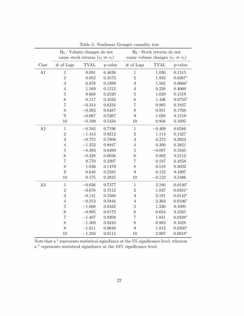
Table 5: Nonlinear Granger causality test

H0 : Volume changes do not H0 : Stock returns do notcause stock returns (vt ; rt) cause volume changes (rt ; vt)

Case # of Lags TVAL p-value # of Lags TVAL p-value

A1 1 0.091 0.4638 1 1.030 0.15152 0.652 0.2573 2 1.932 0.0267∗

3 0.878 0.1899 3 1.502 0.0666†

4 1.169 0.1212 4 0.238 0.40605 0.668 0.2520 5 1.029 0.15186 0.117 0.4533 6 1.436 0.0755†

7 −0.314 0.6234 7 0.905 0.18278 −0.382 0.6487 8 0.951 0.17089 −0.067 0.5267 9 1.028 0.151910 −0.109 0.5434 10 0.956 0.1695

A2 1 −0.582 0.7196 1 −0.409 0.65862 −1.413 0.9212 2 1.114 0.13273 −0.775 0.7809 3 0.273 0.39234 −1.252 0.8947 4 0.300 0.38215 −0.383 0.6493 5 −0.087 0.53456 −0.428 0.6656 6 0.802 0.21127 0.770 0.2207 7 0.187 0.42588 1.046 0.1479 8 0.518 0.30229 0.648 0.2585 9 0.152 0.439710 0.575 0.2825 10 −0.122 0.5486

A3 1 −0.636 0.7377 1 2.180 0.0146∗

2 −0.678 0.7512 2 1.837 0.0331∗

3 −0.141 0.5560 3 2.191 0.0142∗

4 −0.213 0.5844 4 2.303 0.0106∗

5 −1.008 0.8432 5 1.230 0.10956 −0.905 0.8173 6 0.654 0.25657 −1.407 0.9202 7 1.841 0.0328∗

8 −1.569 0.9416 8 0.983 0.16289 −1.811 0.9649 9 1.813 0.0350∗

10 −1.350 0.9115 10 2.907 0.0018∗

Note that a ∗ represents statistical siginifance at the 5% significance level, whereasa † represents statistical siginifance at the 10% significance level.

22

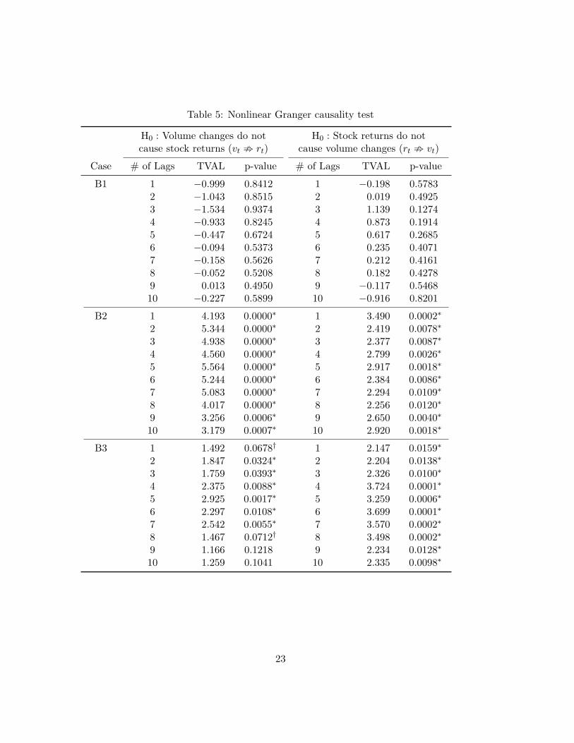
Table 5: Nonlinear Granger causality test

H0 : Volume changes do not H0 : Stock returns do notcause stock returns (vt ; rt) cause volume changes (rt ; vt)

Case # of Lags TVAL p-value # of Lags TVAL p-value

B1 1 −0.999 0.8412 1 −0.198 0.57832 −1.043 0.8515 2 0.019 0.49253 −1.534 0.9374 3 1.139 0.12744 −0.933 0.8245 4 0.873 0.19145 −0.447 0.6724 5 0.617 0.26856 −0.094 0.5373 6 0.235 0.40717 −0.158 0.5626 7 0.212 0.41618 −0.052 0.5208 8 0.182 0.42789 0.013 0.4950 9 −0.117 0.546810 −0.227 0.5899 10 −0.916 0.8201

B2 1 4.193 0.0000∗ 1 3.490 0.0002∗

2 5.344 0.0000∗ 2 2.419 0.0078∗

3 4.938 0.0000∗ 3 2.377 0.0087∗

4 4.560 0.0000∗ 4 2.799 0.0026∗

5 5.564 0.0000∗ 5 2.917 0.0018∗

6 5.244 0.0000∗ 6 2.384 0.0086∗

7 5.083 0.0000∗ 7 2.294 0.0109∗

8 4.017 0.0000∗ 8 2.256 0.0120∗

9 3.256 0.0006∗ 9 2.650 0.0040∗

10 3.179 0.0007∗ 10 2.920 0.0018∗

B3 1 1.492 0.0678† 1 2.147 0.0159∗

2 1.847 0.0324∗ 2 2.204 0.0138∗

3 1.759 0.0393∗ 3 2.326 0.0100∗

4 2.375 0.0088∗ 4 3.724 0.0001∗

5 2.925 0.0017∗ 5 3.259 0.0006∗

6 2.297 0.0108∗ 6 3.699 0.0001∗

7 2.542 0.0055∗ 7 3.570 0.0002∗

8 1.467 0.0712† 8 3.498 0.0002∗

9 1.166 0.1218 9 2.234 0.0128∗

10 1.259 0.1041 10 2.335 0.0098∗

23

Table 5: Nonlinear Granger causality test

H0 : Volume changes do not H0 : Stock returns do notcause stock returns (vt ; rt) cause volume changes (rt ; vt)

Case # of Lags TVAL p-value # of Lags TVAL p-value

C1 1 0.322 0.3738 1 0.451 0.32602 0.885 0.1880 2 −0.512 0.69573 1.234 0.1085 3 −0.436 0.66864 1.377 0.0843† 4 0.560 0.28775 1.265 0.1030 5 0.625 0.26596 1.003 0.1580 6 1.084 0.13937 0.506 0.3065 7 0.239 0.40578 0.537 0.2955 8 0.341 0.36649 0.248 0.4022 9 0.097 0.461210 0.089 0.4644 10 0.158 0.4371

C2 1 0.829 0.2035 1 −2.073 0.98092 −0.462 0.6779 2 −0.149 0.55943 −0.381 0.6484 3 −0.001 0.50034 0.039 0.4845 4 0.282 0.38895 0.518 0.3023 5 −0.358 0.64006 0.219 0.4133 6 −0.518 0.69797 0.178 0.4294 7 −0.421 0.66328 −0.084 0.5334 8 0.709 0.23909 −0.264 0.6040 9 1.238 0.107810 −0.515 0.6967 10 0.860 0.1948

C3 1 −0.833 0.7975 1 −0.686 0.75362 −0.247 0.5976 2 −1.797 0.96393 −0.381 0.6483 3 −0.878 0.81004 −0.854 0.8035 4 0.009 0.49645 −0.983 0.8373 5 0.712 0.23826 −0.751 0.7738 6 0.967 0.16677 −0.177 0.5702 7 0.873 0.19128 −0.084 0.5336 8 1.320 0.0934†

9 −0.316 0.6241 9 2.453 0.0071∗

10 −0.511 0.6955 10 2.069 0.0193∗

24

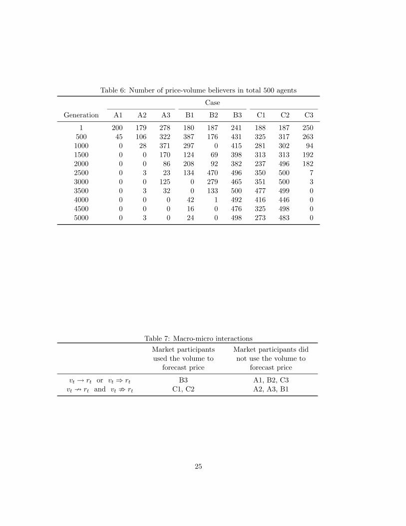
Table 6: Number of price-volume believers in total 500 agents

Case

Generation A1 A2 A3 B1 B2 B3 C1 C2 C3

1 200 179 278 180 187 241 188 187 250500 45 106 322 387 176 431 325 317 2631000 0 28 371 297 0 415 281 302 941500 0 0 170 124 69 398 313 313 1922000 0 0 86 208 92 382 237 496 1822500 0 3 23 134 470 496 350 500 73000 0 0 125 0 279 465 351 500 33500 0 3 32 0 133 500 477 499 04000 0 0 0 42 1 492 416 446 04500 0 0 0 16 0 476 325 498 05000 0 3 0 24 0 498 273 483 0

Table 7: Macro-micro interactionsMarket participants Market participants didused the volume to not use the volume to

forecast price forecast price

vt → rt or vt ⇒ rt B3 A1, B2, C3vt 9 rt and vt ; rt C1, C2 A2, A3, B1

25