Linear Algebraon a

Computer

W. J. Turner

SymbolicComputation

SymbolicAlgorithms

Black BoxMatrix Model

WiedemannMethod

Background

The Method

Linear Algebra on a ComputerAn Introduction to Black Box Methods

William J. Turner

Department of Mathematics & Computer Science

6 February 2007

Linear Algebraon a

Computer

W. J. Turner

SymbolicComputation

SymbolicAlgorithms

Black BoxMatrix Model

WiedemannMethod

Background

The Method

Outline

1 Symbolic Computation

2 Symbolic Algorithms

3 Black Box Matrix Model

4 Wiedemann MethodBackgroundThe Method

Linear Algebraon a

Computer

W. J. Turner

SymbolicComputation

SymbolicAlgorithms

Black BoxMatrix Model

WiedemannMethod

Background

The Method

Symbolic Computation

Superset of computer algebra

Symbols or exact arithmetic

Based on exact finite representation of finite or infinitemathematical objects

Abstract mathematical structures (groups, rings, fields,etc.)

Linear Algebraon a

Computer

W. J. Turner

SymbolicComputation

SymbolicAlgorithms

Black BoxMatrix Model

WiedemannMethod

Background

The Method

Computar Algebra Systems

General Purpose Systems

AXIOM, Magma, Maple, Mathematica, REDUCE

Special Purpose Systems

CoCoA (Computations in Commutative Algebra)

GAP (Groups, Algorithms, and Programming)

NTL (Number Theory Library)

Singular (polynomial computations)

Linear Algebraon a

Computer

W. J. Turner

SymbolicComputation

SymbolicAlgorithms

Black BoxMatrix Model

WiedemannMethod

Background

The Method

Long History

Ancient Algorithms

Euclidean algorithm for finding the greatest commondivisor

Chinese remainder algorithm

Isaac Newton’s The Universal Arithmetic (1728)

Systematically discusses rules for manipulating universalmathematical expressions, that is, formulae containing symbolicindeterminates, and algorithms for solving equations built withthese expressions.

Linear Algebraon a

Computer

W. J. Turner

SymbolicComputation

SymbolicAlgorithms

Black BoxMatrix Model

WiedemannMethod

Background

The Method

Symbolic Computation vs. Numerical Analysis

Numerical Analysis

Floating point numbers (approximate real values)

Find approximation quickly

Error propogation important

Condition Numbers: amplification factors of relative errorsStability: whether all roundoff errors of an algorithm

are harmless

Symbolic Computation

Find exact solution quickly

May never approximate (may have no metric)

Linear Algebraon a

Computer

W. J. Turner

SymbolicComputation

SymbolicAlgorithms

Black BoxMatrix Model

WiedemannMethod

Background

The Method

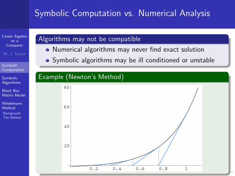
Symbolic Computation vs. Numerical Analysis

Algorithms may not be compatible

Numerical algorithms may never find exact solution

Symbolic algorithms may be ill conditioned or unstable

Example (Newton’s Method)

Linear Algebraon a

Computer

W. J. Turner

SymbolicComputation

SymbolicAlgorithms

Black BoxMatrix Model

WiedemannMethod

Background

The Method

Infinite Mathematical Objects

General Approach

Computer has finite memory

Cannot compute exactly over reals, rationals, integers, etc.

Compute bound on desired solution

Use finite field methods to find solution modulo pi

Reconstruct solution (e.g., Chinese remainder algorithm)

Linear Algebraon a

Computer

W. J. Turner

SymbolicComputation

SymbolicAlgorithms

Black BoxMatrix Model

WiedemannMethod

Background

The Method

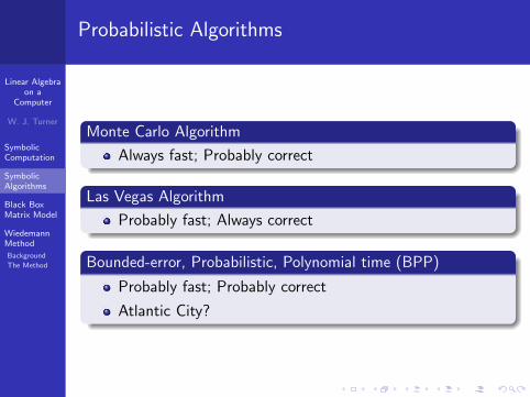
Probabilistic Algorithms

Monte Carlo Algorithm

Always fast; Probably correct

Las Vegas Algorithm

Probably fast; Always correct

Bounded-error, Probabilistic, Polynomial time (BPP)

Probably fast; Probably correct

Atlantic City?

Linear Algebraon a

Computer

W. J. Turner

SymbolicComputation

SymbolicAlgorithms

Black BoxMatrix Model

WiedemannMethod

Background

The Method

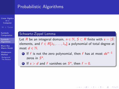
Probabilistic Algorithms

Schwartz-Zippel Lemma

Let R be an integeral domain, n ∈ N, S ⊂ R finite with s = |S |elements, and f ∈ R[λ1, . . . , λn] a polynomial of total degree atmost d ∈ N.

1 If f is not the zero polynomial, then f has at most dsn−1

zeros in Sn.

2 If s > d and f vanishes on Sn, then f = 0.

Linear Algebraon a

Computer

W. J. Turner

SymbolicComputation

SymbolicAlgorithms

Black BoxMatrix Model

WiedemannMethod

Background

The Method

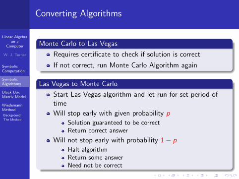
Converting Algorithms

Monte Carlo to Las Vegas

Requires certificate to check if solution is correct

If not correct, run Monte Carlo Algorithm again

Las Vegas to Monte Carlo

Start Las Vegas algorithm and let run for set period oftime

Will stop early with given probability p

Solution guaranteed to be correctReturn correct answer

Will not stop early with probability 1− p

Halt algorithmReturn some answerNeed not be correct

Linear Algebraon a

Computer

W. J. Turner

SymbolicComputation

SymbolicAlgorithms

Black BoxMatrix Model

WiedemannMethod

Background

The Method

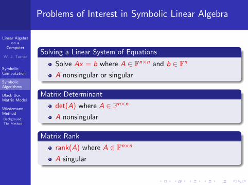
Problems of Interest in Symbolic Linear Algebra

Solving a Linear System of Equations

Solve Ax = b where A ∈ Fn×n and b ∈ Fn

A nonsingular or singular

Matrix Determinant

det(A) where A ∈ Fn×n

A nonsingular

Matrix Rank

rank(A) where A ∈ Fn×n

A singular

Linear Algebraon a

Computer

W. J. Turner

SymbolicComputation

SymbolicAlgorithms

Black BoxMatrix Model

WiedemannMethod

Background

The Method

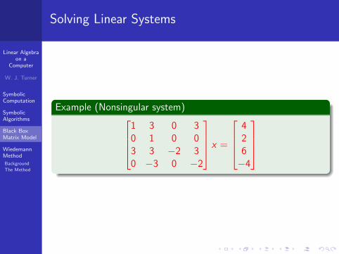
Solving Linear Systems

Example (Nonsingular system)1 3 0 30 1 0 03 3 −2 30 −3 0 −2

x =

426−4

Linear Algebraon a

Computer

W. J. Turner

SymbolicComputation

SymbolicAlgorithms

Black BoxMatrix Model

WiedemannMethod

Background

The Method

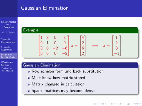
Gaussian Elimination

Example1 3 0 30 1 0 00 0 −2 −60 0 0 −2

x =

4262

=⇒ x =

120−1

Gaussian Elimination

Row echelon form and back substitution

Must know how matrix stored

Matrix changed in calculation

Sparse matrices may become dense

Linear Algebraon a

Computer

W. J. Turner

SymbolicComputation

SymbolicAlgorithms

Black BoxMatrix Model

WiedemannMethod

Background

The Method

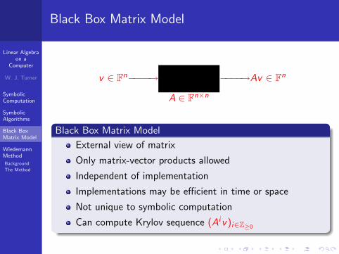
Black Box Matrix Model

v ∈ Fn−−−−→ −−−−→Av ∈ Fn

A ∈ Fn×n

Black Box Matrix Model

External view of matrix

Only matrix-vector products allowed

Independent of implementation

Implementations may be efficient in time or space

Not unique to symbolic computation

Can compute Krylov sequence (Aiv)i∈Z≥0

Linear Algebraon a

Computer

W. J. Turner

SymbolicComputation

SymbolicAlgorithms

Black BoxMatrix Model

WiedemannMethod

Background

The Method

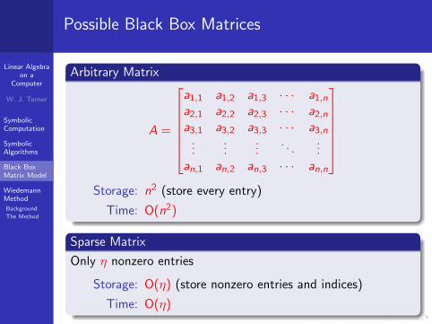
Possible Black Box Matrices

Arbitrary Matrix

A =

a1,1 a1,2 a1,3 · · · a1,n

a2,1 a2,2 a2,3 · · · a2,n

a3,1 a3,2 a3,3 · · · a3,n...

......

. . ....

an,1 an,2 an,3 · · · an,n

Storage: n2 (store every entry)

Time: O(n2)

Sparse Matrix

Only η nonzero entries

Storage: O(η) (store nonzero entries and indices)

Time: O(η)

Linear Algebraon a

Computer

W. J. Turner

SymbolicComputation

SymbolicAlgorithms

Black BoxMatrix Model

WiedemannMethod

Background

The Method

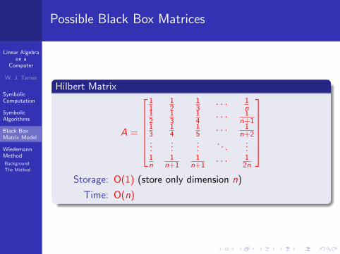
Possible Black Box Matrices

Hilbert Matrix

A =

11

12

13 · · · 1

n12

13

14 · · · 1

n+113

14

15 · · · 1

n+2...

......

. . ....

1n

1n+1

1n+1 · · · 1

2n

Storage: O(1) (store only dimension n)

Time: O(n)

Linear Algebraon a

Computer

W. J. Turner

SymbolicComputation

SymbolicAlgorithms

Black BoxMatrix Model

WiedemannMethod

Background

The Method

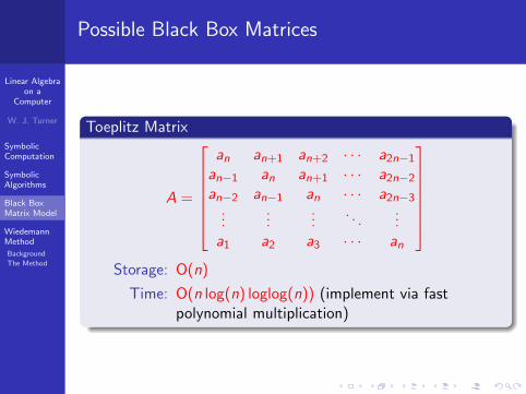
Possible Black Box Matrices

Toeplitz Matrix

A =

an an+1 an+2 · · · a2n−1

an−1 an an+1 · · · a2n−2

an−2 an−1 an · · · a2n−3...

......

. . ....

a1 a2 a3 · · · an

Storage: O(n)

Time: O(n log(n) loglog(n)) (implement via fastpolynomial multiplication)

Linear Algebraon a

Computer

W. J. Turner

SymbolicComputation

SymbolicAlgorithms

Black BoxMatrix Model

WiedemannMethod

Background

The Method

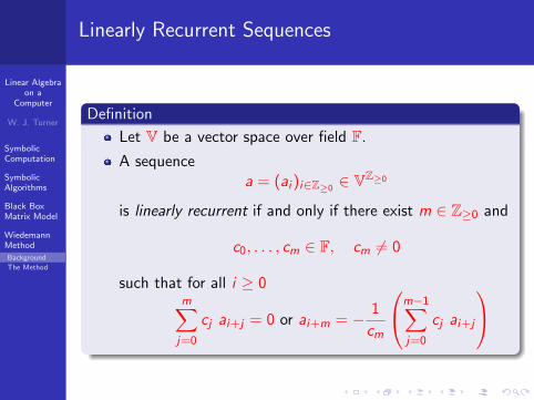
Linearly Recurrent Sequences

Definition

Let V be a vector space over field F.

A sequencea = (ai )i∈Z≥0

∈ VZ≥0

is linearly recurrent if and only if there exist m ∈ Z≥0 and

c0, . . . , cm ∈ F, cm 6= 0

such that for all i ≥ 0m∑

j=0

cj ai+j = 0 or ai+m = − 1

cm

m−1∑j=0

cj ai+j

Linear Algebraon a

Computer

W. J. Turner

SymbolicComputation

SymbolicAlgorithms

Black BoxMatrix Model

WiedemannMethod

Background

The Method

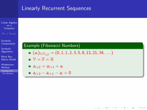
Linearly Recurrent Sequences

Example (Fibonacci Numbers)

(ai )i∈Z≥0= (0, 1, 1, 2, 3, 5, 8, 13, 21, 34, . . . )

V = F = Rai+2 = ai+1 + ai

ai+2 − ai+1 − ai = 0

Linear Algebraon a

Computer

W. J. Turner

SymbolicComputation

SymbolicAlgorithms

Black BoxMatrix Model

WiedemannMethod

Background

The Method

Generating Polynomials

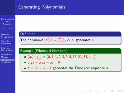
Definition

The polynomial f (λ) =∑m

j=0 cj λj generates a

Example (Fibonacci Numbers)

(ai )i∈Z≥0= (0, 1, 1, 2, 3, 5, 8, 13, 21, 34, . . . )

ai+2 − ai+1 − ai = 0

f = λ2 − λ− 1 generates the Fibonacci sequence a

Linear Algebraon a

Computer

W. J. Turner

SymbolicComputation

SymbolicAlgorithms

Black BoxMatrix Model

WiedemannMethod

Background

The Method

Generating Polynomials

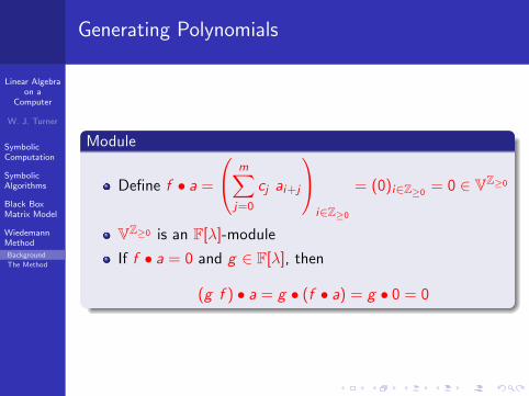
Module

Define f • a =

m∑j=0

cj ai+j

i∈Z≥0

= (0)i∈Z≥0= 0 ∈ VZ≥0

VZ≥0 is an F[λ]-module

If f • a = 0 and g ∈ F[λ], then

(g f ) • a = g • (f • a) = g • 0 = 0

Linear Algebraon a

Computer

W. J. Turner

SymbolicComputation

SymbolicAlgorithms

Black BoxMatrix Model

WiedemannMethod

Background

The Method

Generating Polynomials

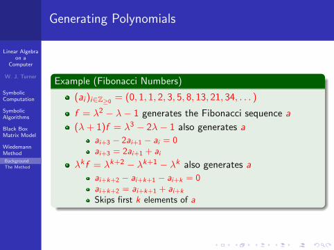
Example (Fibonacci Numbers)

(ai )i∈Z≥0= (0, 1, 1, 2, 3, 5, 8, 13, 21, 34, . . . )

f = λ2 − λ− 1 generates the Fibonacci sequence a

(λ + 1)f = λ3 − 2λ− 1 also generates a

ai+3 − 2ai+1 − ai = 0ai+3 = 2ai+1 + ai

λk f = λk+2 − λk+1 − λk also generates a

ai+k+2 − ai+k+1 − ai+k = 0ai+k+2 = ai+k+1 + ai+k

Skips first k elements of a

Linear Algebraon a

Computer

W. J. Turner

SymbolicComputation

SymbolicAlgorithms

Black BoxMatrix Model

WiedemannMethod

Background

The Method

Minimal Generating Polynomial

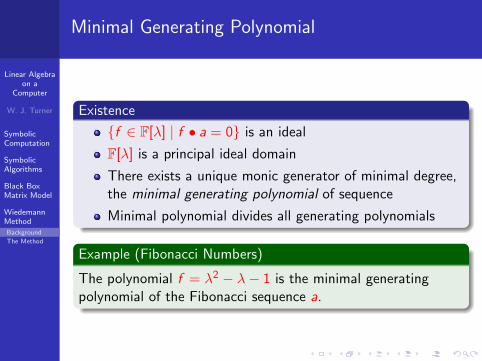
Existence

{f ∈ F[λ] | f • a = 0} is an ideal

F[λ] is a principal ideal domain

There exists a unique monic generator of minimal degree,the minimal generating polynomial of sequence

Minimal polynomial divides all generating polynomials

Example (Fibonacci Numbers)

The polynomial f = λ2 − λ− 1 is the minimal generatingpolynomial of the Fibonacci sequence a.

Linear Algebraon a

Computer

W. J. Turner

SymbolicComputation

SymbolicAlgorithms

Black BoxMatrix Model

WiedemannMethod

Background

The Method

Matrix Power Sequence

Matrix Power Sequence

f • (Ai )i∈Z≥0if and only if f (A) = 0

det(λI − A) generates (Ai )i∈Z≥0

Cayley-Hamilton Theorem

Let f A be the minimal polynomial of (Ai )i∈Z≥0.

f A | det(λI − A)deg(f A) ≤ deg(det(λI − A)) = n

Linear Algebraon a

Computer

W. J. Turner

SymbolicComputation

SymbolicAlgorithms

Black BoxMatrix Model

WiedemannMethod

Background

The Method

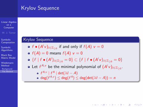
Krylov Sequence

Krylov Sequence

f • (Aiv)i∈Z≥0if and only if f (A) v = 0

f (A) = 0 means f (A) v = 0

{f | f • (Ai )i∈Z≥0= 0} ⊂ {f | f • (Aiv)i∈Z≥0

= 0}Let f A,v be the minimal polynomial of (Aiv)i∈Z≥0

.

f A,v | f A | det(λI − A)deg(f A,v ) ≤ deg(f A) ≤ deg(det(λI − A)) = n

Linear Algebraon a

Computer

W. J. Turner

SymbolicComputation

SymbolicAlgorithms

Black BoxMatrix Model

WiedemannMethod

Background

The Method

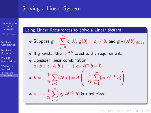
Solving a Linear System

Using Linear Recurrences to Solve a Linear System

Suppose g =m∑

j=0

cj λj , g(0) = c0 6= 0, and g • (Aib)i∈Z≥0

If g exists, then f A,b satisfies the requirements.

Consider linear combinationc0 b + c1 A b + · · ·+ cm Am b = 0

b = − 1

c0

m∑j=1

(Aj b) = A

− 1

c0

m∑j=1

(cj Aj−1 b)

x = − 1

c0

m∑j=1

(cj Aj−1 b) is a solution

Linear Algebraon a

Computer

W. J. Turner

SymbolicComputation

SymbolicAlgorithms

Black BoxMatrix Model

WiedemannMethod

Background

The Method

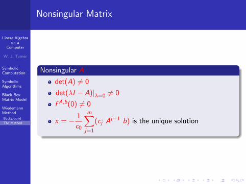
Nonsingular Matrix

Nonsingular A

det(A) 6= 0

det(λI − A)|λ=0 6= 0

f A,b(0) 6= 0

x = − 1

c0

m∑j=1

(cj Aj−1 b) is the unique solution

Linear Algebraon a

Computer

W. J. Turner

SymbolicComputation

SymbolicAlgorithms

Black BoxMatrix Model

WiedemannMethod

Background

The Method

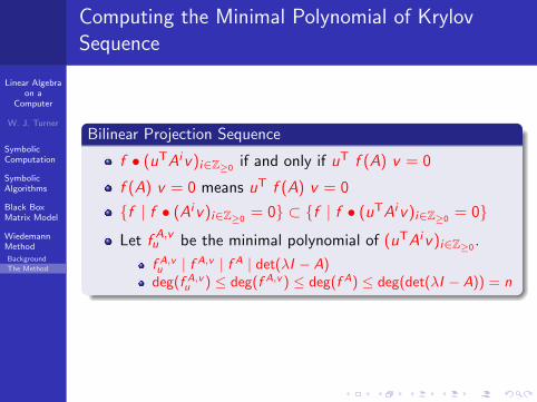
Computing the Minimal Polynomial of KrylovSequence

Bilinear Projection Sequence

f • (uTAiv)i∈Z≥0if and only if uT f (A) v = 0

f (A) v = 0 means uT f (A) v = 0

{f | f • (Aiv)i∈Z≥0= 0} ⊂ {f | f • (uTAiv)i∈Z≥0

= 0}

Let f A,vu be the minimal polynomial of (uTAiv)i∈Z≥0

.

f A,vu | f A,v | f A | det(λI − A)deg(f A,v

u ) ≤ deg(f A,v ) ≤ deg(f A) ≤ deg(det(λI − A)) = n

Linear Algebraon a

Computer

W. J. Turner

SymbolicComputation

SymbolicAlgorithms

Black BoxMatrix Model

WiedemannMethod

Background

The Method

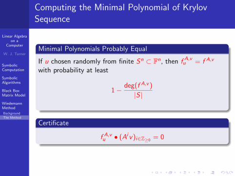
Computing the Minimal Polynomial of KrylovSequence

Minimal Polynomials Probably Equal

If u chosen randomly from finite Sn ⊂ Fn, then f A,vu = f A,v

with probability at least

1− deg(f A,v )

|S |

Certificate

f A,vu • (Aiv)i∈Z≥0

= 0

Linear Algebraon a

Computer

W. J. Turner

SymbolicComputation

SymbolicAlgorithms

Black BoxMatrix Model

WiedemannMethod

Background

The Method

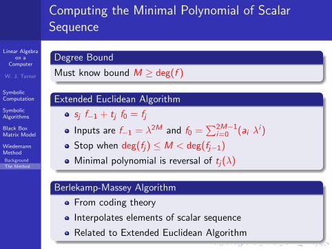
Computing the Minimal Polynomial of ScalarSequence

Degree Bound

Must know bound M ≥ deg(f )

Extended Euclidean Algorithm

sj f−1 + tj f0 = fj

Inputs are f−1 = λ2M and f0 =∑2M−1

i=0 (ai λi )

Stop when deg(fj) ≤ M < deg(fj−1)

Minimal polynomial is reversal of tj(λ)

Berlekamp-Massey Algorithm

From coding theory

Interpolates elements of scalar sequence

Related to Extended Euclidean Algorithm

Linear Algebraon a

Computer

W. J. Turner

SymbolicComputation

SymbolicAlgorithms

Black BoxMatrix Model

WiedemannMethod

Background

The Method

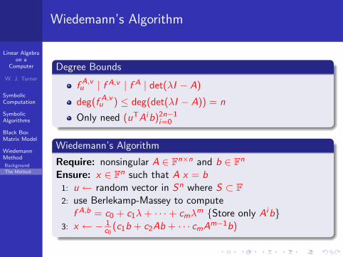
Wiedemann’s Algorithm

Degree Bounds

f A,vu | f A,v | f A | det(λI − A)

deg(f A,vu ) ≤ deg(det(λI − A)) = n

Only need (uTAib)2n−1i=0

Wiedemann’s Algorithm

Require: nonsingular A ∈ Fn×n and b ∈ Fn

Ensure: x ∈ Fn such that A x = b1: u ← random vector in Sn where S ⊂ F2: use Berlekamp-Massey to compute

f A,b = c0 + c1λ + · · ·+ cmλm {Store only Aib}3: x ← − 1

c0(c1b + c2Ab + · · · cmAm−1b)

Linear Algebraon a

Computer

W. J. Turner

SymbolicComputation

SymbolicAlgorithms

Black BoxMatrix Model

WiedemannMethod

Background

The Method

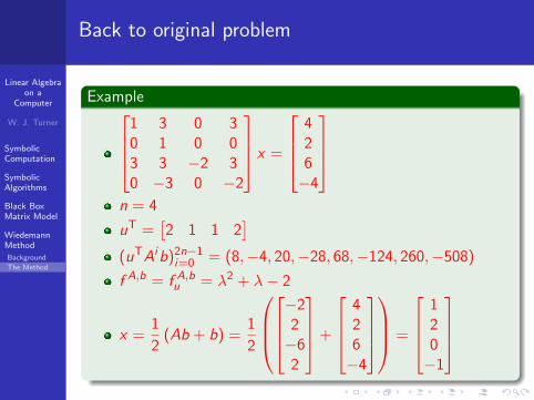
Back to original problem

Example1 3 0 30 1 0 03 3 −2 30 −3 0 −2

x =

426−4

n = 4

uT =[2 1 1 2

](uTAib)2n−1

i=0 = (8,−4, 20,−28, 68,−124, 260,−508)

f A,b = f A,bu = λ2 + λ− 2

x =1

2(Ab + b) =

1

2

−22−62

+

426−4

=

120−1