LINEAR ALGEBRA - oms.bdu.ac.in

LINEAR ALGEBRA Second Edition

KENNETH HOFFMAN Professor of Mathematics Massachusetts Institute of Technology

RAY KUNZE Professor of Mathematics University of California, Irvine

PRENTICE-HALL, INC., Englewood Cliffs, New Jersey

@ 1971, 1961 by Prentice-Hall, Inc. Englewood Cliffs, New Jersey

All rights reserved. No part of this book may be reproduced in any form or by any means without permission in writing from the publisher.

PRENTICE-HALL~NTERNATXONAL,INC., London PRENTICE-HALLOFAUSTRALIA,PTY. LTD., Sydney PRENTICE-HALL OF CANADA, LTD., Toronto PRENTICE-HALLOFINDIA PRIVATE LIMITED, New Delhi PRENTICE-HALL OFJAPAN,INC., Tokyo

Current printing (last digit) :

10 9 8 7 6

Library of Congress Catalog Card No. 75142120 Printed in the United States of America

Pf re ace

Our original purpose in writing this book was to provide a text for the under- graduate linear algebra course at the Massachusetts Institute of Technology. This course was designed for mathematics majors at the junior level, although three- fourths of the students were drawn from other scientific and technological disciplines and ranged from freshmen through graduate students. This description of the M.I.T. audience for the text remains generally accurate today. The ten years since the first edition have seen the proliferation of linear algebra courses throughout the country and have afforded one of the authors the opportunity to teach the basic material to a variety of groups at Brandeis University, Washington Univer- sity (St. Louis), and the University of California (Irvine).

Our principal aim in revising Linear Algebra has been to increase the variety of courses which can easily be taught from it. On one hand, we have structured the chapters, especially the more difficult ones, so that there are several natural stop- ping points along the way, allowing the instructor in a one-quarter or one-semester course to exercise a considerable amount of choice in the subject matter. On the other hand, we have increased the amount of material in the text, so that it can be used for a rather comprehensive one-year course in linear algebra and even as a reference book for mathematicians.

The major changes have been in our treatments of canonical forms and inner product spaces. In Chapter 6 we no longer begin with the general spatial theory which underlies the theory of canonical forms. We first handle characteristic values in relation to triangulation and diagonalization theorems and then build our way up to the general theory. We have split Chapter 8 so that the basic material on inner product spaces and unitary diagonalization is followed by a Chapter 9 which treats sesqui-linear forms and the more sophisticated properties of normal operators, including normal operators on real inner product spaces.

We have also made a number of small changes and improvements from the first edition. But the basic philosophy behind the text is unchanged.

We have made no particular concession to the fact that the majority of the students may not be primarily interested in mathematics. For we believe a mathematics course should not give science, engineering, or social science students a hodgepodge of techniques, but should provide them with an understanding of basic mathematical concepts.

. . . am

Preface

On the other hand, we have been keenly aware of the wide range of back- grounds which the students may possess and, in particular, of the fact that the students have had very little experience with abstract mathematical reasoning. For this reason, we have avoided the introduction of too many abstract ideas at the very beginning of the book. In addition, we have included an Appendix which presents such basic ideas as set, function, and equivalence relation. We have found it most profitable not to dwell on these ideas independently, but to advise the students to read the Appendix when these ideas arise.

Throughout the book we have included a great variety of examples of the important concepts which occur. The study of such examples is of fundamental importance and tends to minimize the number of students who can repeat definition, theorem, proof in logical order without grasping the meaning of the abstract concepts. The book also contains a wide variety of graded exercises (about six hundred), ranging from routine applications to ones which will extend the very best students. These exercises are intended to be an important part of the text.

Chapter 1 deals with systems of linear equations and their solution by means of elementary row operations on matrices. It has been our practice to spend about six lectures on this material. It provides the student with some picture of the origins of linear algebra and with the computational technique necessary to understand examples of the more abstract ideas occurring in the later chapters. Chap- ter 2 deals with vector spaces, subspaces, bases, and dimension. Chapter 3 treats linear transformations, their algebra, their representation by matrices, as well as isomorphism, linear functionals, and dual spaces. Chapter 4 defines the algebra of polynomials over a field, the ideals in that algebra, and the prime factorization of a polynomial. It also deals with roots, Taylor’s formula, and the Lagrange interpolation formula. Chapter 5 develops determinants of square matrices, the determinant being viewed as an alternating n-linear function of the rows of a matrix, and then proceeds to multilinear functions on modules as well as the Grassman ring. The material on modules places the concept of determinant in a wider and more comprehensive setting than is usually found in elementary textbooks. Chapters 6 and 7 contain a discussion of the concepts which are basic to the analysis of a single linear transformation on a finite-dimensional vector space; the analysis of characteristic (eigen) values, triangulable and diagonalizable transformations; the concepts of the diagonalizable and nilpotent parts of a more general transformation, and the rational and Jordan canonical forms. The primary and cyclic decomposition theorems play a central role, the latter being arrived at through the study of admissible subspaces. Chapter 7 includes a discussion of matrices over a polynomial domain, the computation of invariant factors and elementary divisors of a matrix, and the development of the Smith canonical form. The chapter ends with a discussion of semi-simple operators, to round out the analysis of a single operator. Chapter 8 treats finite-dimensional inner product spaces in some detail. It covers the basic geometry, relating orthogonalization to the idea of ‘best approximation to a vector’ and leading to the concepts of the orthogonal projection of a vector onto a subspace and the orthogonal complement of a subspace. The chapter treats unitary operators and culminates in the diagonalization of self-adjoint and normal operators. Chapter 9 introduces sesqui-linear forms, relates them to positive and self-adjoint operators on an inner product space, moves on to the spectral theory of normal operators and then to more sophisticated results concerning normal operators on real or complex inner product spaces. Chapter 10 discusses bilinear forms, emphasizing canonical forms for symmetric and skew-symmetric forms, as well as groups preserving non-degenerate forms, especially the orthogonal, unitary, pseudo-orthogonal and Lorentz groups.

We feel that any course which uses this text should cover Chapters 1, 2, and 3

Preface V

thoroughly, possibly excluding Sections 3.6 and 3.7 which deal with the double dual and the transpose of a linear transformation. Chapters 4 and 5, on polynomials and determinants, may be treated with varying degrees of thoroughness. In fact, polynomial ideals and basic properties of determinants may be covered quite sketchily without serious damage to the flow of the logic in the text; however, our inclination is to deal with these chapters carefully (except the results on modules), because the material illustrates so well the basic ideas of linear algebra. An elementary course may now be concluded nicely with the first four sections of Chap- ter 6, together with (the new) Chapter 8. If the rational and Jordan forms are to be included, a more extensive coverage of Chapter 6 is necessary.

Our indebtedness remains to those who contributed to the first edition, especially to Professors Harry Furstenberg, Louis Howard, Daniel Kan, Edward Thorp, to Mrs. Judith Bowers, Mrs. Betty Ann (Sargent) Rose and Miss Phyllis Ruby. In addition, we would like to thank the many students and colleagues whose per- ceptive comments led to this revision, and the staff of Prentice-Hall for their patience in dealing with two authors caught in the throes of academic administra- tion. Lastly, special thanks are due to Mrs. Sophia Koulouras for both her skill and her tireless efforts in typing the revised manuscript.

K. M. H. / R. A. K.

Contents

Chapter 1. Linear Equations

1.1. Fields 1.2. Systems of Linear Equations 1.3. Matrices and Elementary Row Operations 1.4. Row-Reduced Echelon Matrices 1.5. Matrix Multiplication 1.6. Invertible Matrices

Chapter 2. Vector Spaces

2.1. Vector Spaces 2.2. Subspaces 2.3. Bases and Dimension 2.4. Coordinates 2.5. Summary of Row-Equivalence 2.6. Computations Concerning Subspaces

Chapter 3. Linear Transformations 67

3.1. Linear Transformations 67

3.2. The Algebra of Linear Transformations 74

3.3. Isomorphism 84

3.4. Representation of Transformations by Matrices 86

3.5. Linear Functionals 97

3.6. The Double Dual 107

3.7. The Transpose of a Linear Transformation 111

1

1 3 6

11 16 21

28

28 34 40 49 55 58

Vi

Contents vii

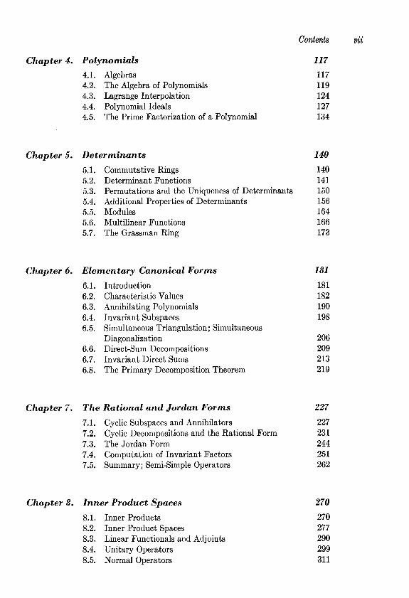
Chapter 4. Polynomials

4.1. Algebras 4.2. The Algebra of Polynomials 4.3. Lagrange Interpolation 4.4. Polynomial Ideals 4.5. The Prime Factorization of a Polynomial

117

117 119 124 127 134

Chapter 5. Determinants 140

5.1. Commutative Rings 140

5.2. Determinant Functions 141 5.3. Permutations and the Uniqueness of Determinants 150 5.4. Additional Properties of Determinants 156

5.5. Modules 164 5.6. Multilinear Functions 166 5.7. The Grassman Ring 173

Chapter 6. Elementary Canonical Forms

6.1. Introduction 6.2. Characteristic Values 6.3. Annihilating Polynomials 6.4. Invariant Subspaces 6.5. Simultaneous Triangulation; Simultaneous

Diagonalization 6.6. Direct-Sum Decompositions 6.7. Invariant Direct Sums 6.8. The Primary Decomposition Theorem

181

181 182 190 198

206 209 213 219

Chapter 7. The Rational and Jordan Forms 227

7.1. Cyclic Subspaces and Annihilators 227

7.2. Cyclic Decompositions and the Rational Form 231

7.3. The Jordan Form 244

7.4. Computation of Invariant Factors 251 7.5. Summary; Semi-Simple Operators 262

Chapter 8. Inner Product Spaces

8.1. Inner Products 8.2. Inner Product Spaces 8.3. Linear Functionals and Adjoints 8.4. Unitary Operators 8.5. Normal Operators

270

270 277 290 299 311

Sec. 1.2 Systems of Linear Equations 3

-1. With the usual operations of addition and multiplication, the set of integers satisfies all of the conditions (l)-(9) except condition (8).

EXAMPLE 3. The set of rational numbers, that is, numbers of the form p/q, where p and q are integers and q # 0, is a subfield of the field of complex numbers. The division which is not possible within the set of integers is possible within the set of rational numbers. The interested reader should verify that any subfield of C must contain every rational number.

EXAMPLE 4. The set of all complex numbers of the form 2 + yG, where x and y are rational, is a subfield of C. We leave it to the reader to verify this.

In the examples and exercises of this book, the reader should assume that the field involved is a subfield of the complex numbers, unless it is expressly stated that the field is more general. We do not want to dwell on this point; however, we should indicate why we adopt such a conven- tion. If F is a field, it may be possible to add the unit 1 to itself a finite number of times and obtain 0 (see Exercise 5 following Section 1.2) :

1+ 1 + ... + 1 = 0.

That does not happen in the complex number field (or in any subfield thereof). If it does happen in F, then the least n such that the sum of n l’s is 0 is called the characteristic of the field F. If it does not happen in F, then (for some strange reason) F is called a field of characteristic

zero. Often, when we assume F is a subfield of C, what we want to guaran- tee is that F is a field of characteristic zero; but, in a first exposure to linear algebra, it is usually better not to worry too much about charac- teristics of fields.

1.2. Systems of Linear Equations

Suppose F is a field. We consider the problem of finding n scalars (elements of F) x1, . . . , x, which satisfy the conditions

&Xl + A12x2 + .-a + Al?& = y1

(l-1) &XI + &x2 + ... + Aznxn = y2

A :,x:1 + A,zxz + . . . + A;nxn = j_

where yl, . . . , ym and Ai?, 1 5 i 5 m, 1 5 j 5 n, are given elements of F. We call (l-l) a system of m linear equations in n unknowns.

Any n-tuple (xi, . . . , x,) of elements of F which satisfies each of the

Linear Equations Chap. 1

equations in (l-l) is called a solution of the system. If yl = yZ = . . . = ym = 0, we say that the system is homogeneous, or that each of the equations is homogeneous.

Perhaps the most fundamental technique for finding the solutions of a system of linear equations is the technique of elimination. We can illustrate this technique on the homogeneous system

2x1 - x2 + x3 = 0

x1 + 322 + 4x3 = 0.

If we add (-2) times the second equation to the first equation, we obtain

-7X2 - 723 = 0

or, x2 = -x3. If we add 3 times the first equation to the second equation, we obtain

7x1 + 7x3 = 0

or, x1 = -x3. So we conclude that if (xl, x2, x3) is a solution then x1 = x2 = -x3. Conversely, one can readily verify that any such triple is a solution. Thus the set of solutions consists of all triples (-a, -a, a).

We found the solutions to this system of equations by ‘eliminating unknowns,’ that is, by multiplying equations by scalars and then adding to produce equations in which some of the xj were not present. We wish to formalize this process slightly so that we may understand why it works, and so that we may carry out the computations necessary to solve a system in an organized manner.

For the general system (l-l), suppose we select m scalars cl, . . . , c,, multiply the jth equation by ci and then add. We obtain the equation

(Cl& + . . . + CmAml)Xl + . . * + (Cl&a + . . . + c,A,n)xn

= c1y1 + . . . + G&7‘.

Such an equation we shall call a linear combination of the equations in (l-l). Evidently, any solution of the entire system of equations (l-l) will also be a solution of this new equation. This is the fundamental idea of the elimination process. If we have another system of linear equations

&1X1 + . . . + BlnXn = Xl

U-2) &-lx1 + . * . + Bk’nxn = z,,

in which each of the k equations is a linear combination of the equations in (l-l), then every solution of (l-l) is a solution of this new system. Of course it may happen that some solutions of (l-2) are not solutions of (l-l). This clearly does not happen if each equation in the original system is a linear combination of the equations in the new system. Let us say that two systems of linear equations are equivalent if each equation in each system is a linear combination of the equations in the other system. We can then formally state our observations as follows.

Sec. 1.2 Systems of Linear Equations 5

Theorem 1. Equivalent systems of linear equations have exactly the same solutions.

If the elimination process is to be effective in finding the solutions of

a system like (l-l), then one must see how, by forming linear combina-

tions of the given equations, to produce an equivalent system of equations

which is easier to solve. In the next section we shall discuss one method

of doing this.

Exercises

1. Verify that the set of complex numbers described in Example 4 is a subfield of C.

2. Let F be the field of complex numbers. Are the following two systems of linear equations equivalent? If so, express each equation in each system as a linear combination of the equations in the other system.

Xl - x2 = 0 321 + x2 = 0 2x1 + x2 = 0 Xl + x2 = 0

3. Test the following systems of equations as in Exercise 2.

-x1 + x2 + 4x3 = 0 21 - 23 = 0 x1 + 3x2 + 8x3 = 0 x2 + 3x8 = 0

&Xl + x2 + 5x3 = 0

4. Test the following systems as in Exercise 2.

2x1 + (- 1 + i)x2 + x4=0 ( I

1 + i x1 + 8x2 - ixg - x4 = 0

3x2 - %x3 + 5x4 = 0 +x1 - gx, + x3 + 7x4 = 0

5. Let F be a set which contains exactly two elements, 0 and 1. Define an addition and multiplication by the tables:

+ 0 1 .Ol --

0 0 1 0 00 110 101

Verify that the set F, together with these two operations, is a field.

6. Prove that if two homogeneous systems of linear equations in two unknowns have the same solutions, then they are equivalent.

7. Prove that each subfield of the field of complex numbers contains every rational number.

8. Prove that each field of characteristic zero contains a copy of the rational number field.

6 Linear Equations Chap. 1

1.3. Matrices and Elementary

Row Operations

One cannot fail to notice that in forming linear combinations of linear equations there is no need to continue writing the ‘unknowns’

. . , GL, since one actually computes only with the coefficients Aij and Fie’ scalars yi. We shall now abbreviate the system (l-l) by

AX = Y where

11 *** -4.1,

[: :I A,1 . -a A’,,

x=;;,A Yl

and Y = : [ ] .

Ym We call A the matrix of coefficients of the system. Strictly speaking, the rectangular array displayed above is not a matrix, but is a representation of a matrix. An m X n matrix over the field F is a function A from the set of pairs of integers (i, j), 1 5 i < m, 1 5 j 5 n, into the field F. The entries of the matrix A are the scalars A (i, j) = Aij, and quite often it is most convenient to describe the matrix by displaying its entries in a rectangular array having m rows and n columns, as above. Thus X (above) is, or defines, an n X 1 matrix and Y is an m X 1 matrix. For the time being, AX = Y is nothing more than a shorthand notation for our system of linear equations. Later, when we have defined a multiplication for matrices, it will mean that Y is the product of A and X.

We wish now to consider operations on the rows of the matrix A which correspond to forming linear combinations of the equations in the system AX = Y. We restrict our attention to three elementary row

operations on an m X n matrix A over the field F:

1. multiplication of one row of A by a non-zero scalar c; 2. replacement of the rth row of A by row r plus c times row s, c any

scalar and r # s; 3. interchange of two rows of A.

An elementary row operation is thus a special type of function (rule) e which associated with each m X n matrix A an m X n matrix e(A). One can precisely describe e in the three cases as follows:

1. e(A)ii = Aii if i # T, e(A)7j = cAyi. 2. e(A)ij = A+ if i # r, e(A)?j = A,i + cA,~.

3. e(A)ij = Aij if i is different from both r and s, e(A),j = A,j, e(A)8j = A,+

Sec. 1.3 Matrices and Elementary Row Operations 7

In defining e(A), it is not really important how many columns A has, but the number of rows of A is crucial. For example, one must worry a little to decide what is meant by interchanging rows 5 and 6 of a 5 X 5 matrix. To avoid any such complications, we shall agree that an elementary row operation e is defined on the class of all m X n matrices over F, for some fixed m but any n. In other words, a particular e is defined on the class of all m-rowed matrices over F.

One reason that we restrict ourselves to these three simple types of row operations is that, having performed such an operation e on a matrix A, we can recapture A by performing a similar operation on e(A).

Theorem 2. To each elementary row operation e there corresponds an elementary row operation el, of the same type as e, such that el(e(A)) = e(el(A)) = A for each A, In other words, the inverse operation (junction) of an elementary row operation exists and is an elementary row operation of the same type.

Proof. (1) Suppose e is the operation which multiplies the rth row of a matrix by the non-zero scalar c. Let el be the operation which multiplies row r by c-l. (2) Suppose e is the operation which replaces row r by row r plus c times row s, r # s. Let el be the operation which replaces row r by row r plus (-c) times row s. (3) If e interchanges rows r and s, let el = e. In each of these three cases we clearly have ei(e(A)) = e(el(A)) = A for each A. 1

Dejinition. If A and B are m X n matrices over the jield F, we say that B is row-equivalent to A if B can be obtained from A by a$nite sequence of elementary row operations.

Using Theorem 2, the reader should find it easy to verify the following. Each matrix is row-equivalent to itself; if B is row-equivalent to A, then A is row-equivalent to B; if B is row-equivalent to A and C is row-equivalent to B, then C is row-equivalent to A. In other words, row-equivalence is an equivalence relation (see Appendix).

Theorem 3. If A and B are row-equivalent m X n matrices, the homogeneous systems of linear equations Ax = 0 and BX = 0 have exactly the same solutions.

Proof. Suppose we pass from A to B by a finite sequence of elementary row operations:

A = A,,+A1+ ... +Ak = B.

It is enough to prove that the systems AjX = 0 and Aj+lX = 0 have the same solutions, i.e., that one elementary row operation does not disturb the set of solutions.


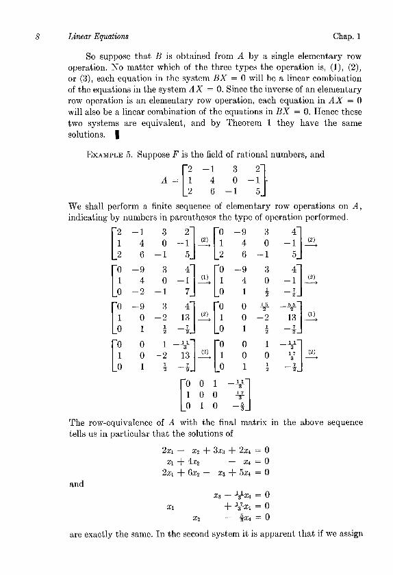
So suppose that B is obtained from A by a single elementary row operation. No matter which of the three types the operation is, (l), (2), or (3), each equation in the system BX = 0 will be a linear combination of the equations in the system AX = 0. Since the inverse of an elementary row operation is an elementary row operation, each equation in AX = 0 will also be a linear combination of the equations in BX = 0. Hence these two systems are equivalent, and by Theorem 1 they have the same solutions. 1

EXAMPLE 5. Suppose F is the field of rational numbers, and

We shall perform a finite sequence of elementary row operations on A, indicating by numbers in parentheses the type of operation performed.

6-l 5

The row-equivalence of A with the final matrix in the above sequence tells us in particular that the solutions of

2x1 - x2 + 3x3 + 2x4 = 0 xl + 4x2 - x4 = 0

2x1 + 6x2 - ~3 + 5x4 = 0 and

x3 - 9x4 = 0 Xl +yx4=0

x2 5x -0 - g4-

are exactly the same. In the second system it is apparent that if we assign

Sec. 1.3 Matrices and Elementary Row Operations

any rational value c to x4 we obtain a solution (-+c, %, J+c, c), and also that every solution is of this form.

EXAMPLE 6. Suppose F is the field of complex numbers and

Thus the system of equations

-51 + ix, = 0 --ix1 + 3x2 = 0

x1 + 2x2 = 0

has only the trivial solution x1 = x2 = 0.

In Examples 5 and 6 we were obviously not performing row operations at random. Our choice of row operations was motivated by a desire to simplify the coefficient matrix in a manner analogous to ‘eliminating unknowns’ in the system of linear equations. Let us now make a formal definition of the type of matrix at which we were attempting to arrive.

DeJinition. An m X n matrix R is called row-reduced if:

(a) the jirst non-zero entry in each non-zero row of R is equal to 1; (b) each column of R which contains the leading non-zero entry of some

row has all its other entries 0.

EXAMPLE 7. One example of a row-reduced matrix is the n X n (square) identity matrix I. This is the n X n matrix defined by

Iii = 6,j = -t

1, if i=j 0, if i # j.

This is the first of many occasions on which we shall use the Kronecker

delta (6).

In Examples 5 and 6, the final matrices in the sequences exhibited there are row-reduced matrices. Two examples of matrices which are not row-reduced are:


The second matrix fails to satisfy condition (a), because the leading non- zero entry of the first row is not 1. The first matrix does satisfy condition (a), but fails to satisfy condition (b) in column 3.

We shall now prove that we can pass from any given matrix to a row- reduced matrix, by means of a finite number of elementary row oper- tions. In combination with Theorem 3, this will provide us with an effective tool for solving systems of linear equations.

Theorem 4. Every m X n matrix over the field F is row-equivalent to a row-reduced matrix.

Proof. Let A be an m X n matrix over F. If every entry in the first row of A is 0, then condition (a) is satisfied in so far as row 1 is con- cerned. If row 1 has a non-zero entry, let k be the smallest positive integer j for which Alj # 0. Multiply row 1 by AG’, and then condition (a) is satisfied with regard to row 1. Now for each i 2 2, add (-Aik) times row 1 to row i. Now the leading non-zero entry of row 1 occurs in column k, that entry is 1, and every other entry in column k is 0.

Now consider the matrix which has resulted from above. If every entry in row 2 is 0, we do nothing to row 2. If some entry in row 2 is different from 0, we multiply row 2 by a scalar so that the leading non-zero entry is 1. In the event that row 1 had a leading non-zero entry in column k, this leading non-zero entry of row 2 cannot occur in column k; say it occurs in column Ic, # k. By adding suitable multiples of row 2 to the various rows, we can arrange that all entries in column k’ are 0, except the 1 in row 2. The important thing to notice is this: In carrying out these last operations, we will not change the entries of row 1 in columns 1, . . . , k; nor will we change any entry of column k. Of course, if row 1 was identically 0, the operations with row 2 will not affect row 1.

Working with one row at a time in the above manner, it is clear that in a finite number of steps we will arrive at a row-reduced matrix. 1

Exercises

1. Find all solutions to the system of equations

(1 - i)Zl - ixz = 0 2x1 + (1 - i)zz = 0.

2. If 3 -1 2

A=2 [ 11 1 1 -3 0

find all solutions of AX = 0 by row-reducing A.

Sec. 1.4 Row-Reduced Echelon Matrices 11

3. If

find all solutions of AX = 2X and all solutions of AX = 3X. (The symbol cX denotes the matrix each entry of which is c times the corresponding entry of X.)

4. Find a row-reduced matrix which is row-equivalent to

6. Let

be a 2 X 2 matrix with complex entries. Suppose that A is row-reduced and also that a + b + c + d = 0. Prove that there are exactly three such matrices.

7. Prove that the interchange of two rows of a matrix can be accomplished by a finite sequence of elementary row operations of the other two types.

8. Consider the system of equations AX = 0 where

is a 2 X 2 matrix over the field F. Prove the following. (a) If every entry of A is 0, then every pair (xi, Q) is a solution of AX = 0. (b) If ad - bc # 0, the system AX = 0 has only the trivial solution z1 =

x2 = 0. (c) If ad - bc = 0 and some entry of A is different from 0, then there is a

solution (z:, x20) such that (xi, 22) is a solution if and only if there is a scalar y such that zrl = yxy, x2 = yxg.

1 .P. Row-Reduced Echelon Matrices

Until now, our work with systems of linear equations was motivated by an attempt to find the solutions of such a system. In Section 1.3 we established a standardized technique for finding these solutions. We wish now to acquire some information which is slightly more theoretical, and for that purpose it is convenient to go a little beyond row-reduced matrices.

DeJinition. An m X n matrix R is called a row-reduced echelon matrix if:


(a) R is row-reduced; (b) every row of R which has all its entries 0 occurs below every row

which has a non-zero entry; (c) ifrowsl,..., r are the non-zero rows of R, and if the leading non-

zero entry of row i occurs in column ki, i = 1, . . . , r, then kl < kz < . . . < k,.

One can also describe an m X n row-reduced echelon matrix R as follows. Either every entry in R is 0, or there exists a positive integer r, 1 5 r 5 m, and r positive integers kl, . . . , k, with 1 5 ki I: n and

(a) Rij=Ofori>r,andRij=Oifj<k;. (b) &ki = 8ij, 1 5 i 5 r, 1 5 j 5 r. (c) kl < . . . < k,.

EXAMPLE 8. Two examples of row-reduced echelon matrices are the n X n identity matrix, and the m X n zero matrix O”J’, in which all entries are 0. The reader should have no difficulty in making other examples, but we should like to give one non-trivial one:

Theorem 5. Every m X n matrix A is row-equivalent to a row-reduced echelon matrix.

Proof. We know that A is row-equivalent to a row-reduced matrix. All that we need observe is that by performing a finite number of row interchanges on a row-reduced matrix we can bring it to row-reduced echelon form. 1

In Examples 5 and 6, we saw the significance of row-reduced matrices in solving homogeneous systems of linear equations. Let us now discuss briefly the system RX = 0, when R is a row-reduced echelon matrix. Let rows 1, . . . , r be the non-zero rows of R, and suppose that the leading non-zero entry of row i occurs in column ki. The system RX = 0 then consists of r non-trivial equations. Also the unknown xk; will occur (with non-zero coefficient) only in the ith equation. If we let ul, . . . , u+,. denote the (n - r) unknowns which are different from xk,, . . . , xk,, then the r non-trivial equations in RX = 0 are of the form

Xkl + Z CljUj = 0

(l-3) . j=l

n--r Xk, -I- Z CrjUj = 0.

j=l

Sec. 1.4 Row-Reduced Echelon Matrices

All the solutions to the system of equations RX = 0 are obtained by assigning any values whatsoever to ~1, . . . , u,-, and then computing the corresponding values of xk,, . . . , xk, from (l-3). For example, if R is the matrix displayed in Example 8, then r = 2, ICI = 2, i& = 4, and the two non-trivial equations in the system RX = 0 are

x2 - 3x3 + $x5 = 0 or x2 = 3x3 - +x5 x4+2x5=0 or x4= -2x5.

So we may assign any values to xi, x3, and x5, say x1 = a, 23 = b, x5 = c, and obtain the solution (a, 3b - +c, 6, -2c, c).

Let us observe one thing more in connection with the system of equations RX = 0. If the number r of non-zero rows in R is less than n, then the system RX = 0 has a non-trivial solution, that is, a solution (Xl, . . . ) x,) in which not every xi is 0. For, since r < n, we can choose some Xj which is not among the r unknowns xk,, . . . , xk,, and we can then construct a solution as above in which this xi is 1. This observation leads us to one of the most fundamental facts concerning systems of homogeneous linear equations.

Theorem 6. Zf A is an m X n matrix and m < n, then the homogeneous system of linear equations Ax = 0 has a non-trivial solution.

Proof. Let R be a row-reduced echelon matrix which is row- equivalent to A. Then the systems AX = 0 and RX = 0 have the same solutions by Theorem 3. If r is the number of rows in R, then certainly r 5 m, and since m < n, we have r < n. It follows immediately from our remarks above that AX = 0 has a non-trivial solution. 1

Theorem 7. Zf A is an n X n (square) matrix, then A is row-equivalent to the n X n identity matrix if and only if the system of equations AX = 0 has only the trivial solution.

Proof. If A is row-equivalent to I, then AX = 0 and IX = 0 have the same solutions. Conversely, suppose AX = 0 has only the trivial solution X = 0. Let R be an n X n row-reduced echelon matrix which is row-equivalent to A, and let r be the number of non-zero rows of R. Then RX = 0 has no non-trivial solution. Thus r 2 n. But since R has n rows, certainly r < n, and we have r = n. Since this means that R actually has a leading non-zero entry of 1 in each of its n rows, and since these l’s occur each in a different one of the n columns, R must be the n X n identity matrix. 1

Let us now ask what elementary row operations do toward solving a system of linear equations AX = Y which is not homogeneous. At the outset, one must observe one basic difference between this and the homogeneous case, namely, that while the homogeneous system always has the


trivial solution 51 = . . . = x, = 0, an inhomogeneous system need have no solution at all.

We form the augmented matrix A’ of the system AX = Y. This is the m X (n + 1) matrix whose first n columns are the columns of A and whose last column is Y. More precisely,

A& = Aii, if j 5 n Ai(n+l) = Yi.

Suppose we perform a sequence of elementary row operations on A, arriving at a row-reduced echelon matrix R. If we perform this same sequence of row operations on the augmented matrix A’, we will arrive at a matrix R’ whose first n columns are the columns of R and whose last column contains certain scalars 21, . . . , 2,. The scalars xi are the entries of the m X 1 matrix 21 z= ; [I Gn which results from applying the sequence of row operations to the matrix Y. It should be clear to the reader that, just as in the proof of Theorem 3, the systems AX = Y and RX = Z are equivalent and hence have the same solutions. It is very easy to determine whether the system RX = Z has any solutions and to determine all the solutions if any exist. For, if R has r non-zero rows, with the leading non-zero entry of row i occurring in column ki, i = 1, . . . , rr then the first r equations of RX = Z effec- tively express zk,, . . . , xk, in terms of the (n - r) remaining xj and the scalars zl, . . . , zT. The last (m - r) equations are

0 = G+1

and accordingly the condition for the system to have a solution is zi = 0 for i > r. If this condition is satisfied, all solutions to the system are found just as in the homogeneous case, by assigning arbitrary values to (n - r) of the xj and then computing xk; from the ith equation.

EXAMPLE 9. Let F be the field of rational numbers and

and suppose that we wish to solve the system AX = Y for some yl, yz, and y3. Let us perform a sequence of row operations on the augmented matrix A’ which row-reduces A :

Sec. 1.4 Row-Reduced Echelon Matrices 15

E -; -i p E -i j (yz $24 3

[

1 -2 1 Yl l-2 1 Yl 0 5 -1 (Y/z - 2?/1)

I [

(1!0 1 -* gyz - Q> (2! ’ 0 0 0 (y3 - yz + 2Yd 0 0 0 (ya - yz + 2%) 1

[ 10 Q 3CYl + 2Yz) 0 1 -4 icy2 - &/I) . 0 0 0 (Y3 - y2 + 2Yl) I

The condition that the system AX = Y have a solution is thus

2Yl - yz + y3 = 0

and if the given scalars yi satisfy this condition, all solutions are obtained by assigning a value c to x3 and then computing

x1 = -$c + Q(y1 + 2Yd 22 = Bc + tcyz - 2Yd.

Let us observe one final thing about the system AX = Y. Suppose the entries of the matrix A and the scalars yl, . . . , ym happen to lie in a sibfield Fl of the field F. If the system of equations AX = Y has a solution with x1, . . . , x, in F, it has a solution with x1, . . . , xn in Fl. F’or, over either field, the condition for the system to have a solution is that certain relations hold between ~1, . . . , ym in FI (the relations zi = 0 for i > T, above). For example, if AX = Y is a system of linear equations in which the scalars yk and Aij are real numbers, and if there is a solution in which x1, . . . , xn are complex numbers, then there is a solution with 21, . . . , xn real numbers.

Exercises

1. Find all solutions to the following system of equations by row-reducing the coefficient matrix:

;a + 2x2 - 6x3 = 0 -4x1 + 55.7 = 0 -3x1 + 622 - 13x3 = 0 -$x1+ 2x2 - *x - 0 73-

2. Find a row-reduced echelon matrix which is row-equivalent to 1 . A=2 ;“. [ 1 i 1+i

What are the solutions of AX = O?


3. Describe explicitly all 2 X 2 row-reduced echelon matrices.

4. Consider the system of equations

Xl - x2 + 2x3 = 1 2x1 + 2x3 = 1

Xl - 3x2 + 4x3 = 2.

Does this system have a solution? If so, describe explicitly all solutions.

5. Give an example of a system of two linear equations in two unknowns which has no solution.

6. Show that the system

Xl - 2x2 + x3 + 2x4 = 1 Xl + X2 - x3 + xp = 2 21 + 7X2 - 5X3 - X4 = 3

has no solution.

7. Find all solutions of

2~~-3~~-7~~+5~4+2x~= -2 ZI-~XZ-~X~+~X~+ x5= -2

2x1 -4X3+2X4+ 25 = 3

XI - 5X2 - 7x3 + 6x4 + 2x5 = -7.

8. Let 3 -1 2

A=2 11. [ 1 1 -3 0

For which triples (yr, y2, y3) does the system AX = Y have a solution?

9. Let 3 -6 2 -1

For which (~1, y2, y3, y4) does the system of equations AX = Y have a solution?

10. Suppose R and R’ are 2 X 3 row-reduced echelon matrices and that the systems RX = 0 and R’X = 0 have exactly the same solutions. Prove that R = R’.

1.5. Matrix Multiplication

It is apparent (or should be, at any rate) that the process of forming linear combinations of the rows of a matrix is a fundamental one. For this reason it is advantageous to introduce a systematic scheme for indicating just what operations are to be performed. More specifically, suppose B is an n X p matrix over a field F with rows PI, . . . , Pn and that from B we construct a matrix C with rows 71, . . . , yrn by forming certain linear combinations

(l-4) yi = Ail/G + A& + . . . + AinPn.

Sec. 1.5 Matrix Multiplication 17

The rows of C are determined by the mn scalars Aij which are themselves the entries of an m X n matrix A. If (l-4) is expanded to

(Gil * * .Ci,> = i 64i,B,1. . . Air&p) r=l

we see that the entries of C are given by

Cij = 5 Ai,Brj. r=l

DeJnition. Let A be an m X n matrix over the jield F and let R be an n X p matrix over I?. The product AB is the m X p matrix C whose i, j entry is

Cij = 5 Ai,B,j. r=l

EXAMPLE 10. Here are some products of matrices with rational entries.

(4 [; -: ;I = [ -5 ;I [l; -: ;I Here

Yl = (5 -1 2) = 1 . (5 -1 2) + 0. (15 4 8) Y-2 = (0 7 2) = -3(5 -1 2) + 1 . (15 4 8)

Cb) [I; ; Ii] = [-i gK s” -8-l

Here yz=(9 12 -8) = -2(O 6 1) + 3(3 8 -2) 73 = (12 62 -3) = 5(0 6 1) + 4(3 8 -2)

cc>

(4

[2i] = [i Xl [-; J=[-$2 41

Here yz = (6 12) = 3(2 4)

(0

k>

[ 0 2 0 0 0 3 4 0 0 1 [ 0 0 0 9 2 1 0 0 0 1

Linear Equations Chap. 1

It is important to observe that the product of two matrices need not be defined; the product is defined if and only if the number of columns in the first matrix coincides with the number of rows in the second matrix. Thus it is meaningless to interchange the order of the factors in (a), (b), and (c) above. Frequently we shall write products such as AB without explicitly mentioning the sizes of the factors and in such cases it will be understood that the product is defined. From (d), (e), (f), (g) we find that even when the products AB and BA are both defined it need not be true that AB = BA; in other words, matrix multiplication is not commutative.

EXAMPLE 11.

(a) If I is the m X m identity matrix and A is an m X n matrix, IA=A.

(b) If I is the n X n identity matrix and A is an m X n matrix, AI = A.

(c) If Ok+ is the k X m zero matrix, Ok+ = OksmA. Similarly, ‘4@BP = ()%P.

EXAMPLE 12. Let A be an m X n matrix over F. Our earlier shorthand notation, AX = Y, for systems of linear equations is consistent with our definition of matrix products. For if

Xl

x= “.” [:I &I

with xi in F, then AX is the m X 1 matrix

Yl

y= y.” [:I Ym

such that yi = Ails1 + Ai2~2 + . . . + Ai,x,. The use of column matrices suggests a notation which is frequently

useful. If B is an n X p matrix, the columns of B are the 1 X n matrices BI,. . . , BP defined by

lljip.

The matrix B is the succession of these columns:

B = [BI, . . . , BP].

The i, j entry of the product matrix AB is formed from the ith row of A

Sec. 1.5 Matrix Multiplication 19

and the jth column of B. The reader should verify that the jth column of AB is AB,:

AB = [ABI, . . . , A&].

In spite of the fact that a product of matrices depends upon the order in which the factors are written, it is independent of the way in which they are associated, as the next theorem shows.

Theorem 8. If A, B, C are matrices over the field F such that the products BC and A(BC) are defined, then so are the products AB, (AB)C and

A(BC) = (AB)C.

Proof. Suppose B is an n X p matrix. Since BC is defined, C is a matrix with p rows, and BC has n rows. Because A(BC) is defined we may assume A is an m X n matrix. Thus the product AB exists and is an m X p matrix, from which it follows that the product (AB)C exists. To show that A(BC) = (AB)C means to show that

[A(BC)lij = [W)Clij

for each i, j. By definition

[A(BC)]ij = Z A+(BC)rj

= d AC 2 BmCnj

= 6 Z AbmCsj r 8

= 2 (AB)i,C,j 8

= [(AB)C’]ij. 1

When A is an n X n (square) matrix, the product AA is defined. We shall denote this matrix by A 2. By Theorem 8, (AA)A = A(AA) or A2A = AA2, so that the product AAA is unambiguously defined. This product we denote by A3. In general, the product AA . . . A (k times) is unambiguously defined, and we shall denote this product by A”.

Note that the relation A(BC) = (AB)C implies among other things that linear combinations of linear combinations of the rows of C are again linear combinations of the rows of C.

If B is a given matrix and C is obtained from B by means of an elementary row operation, then each row of C is a linear combination of the rows of B, and hence there is a matrix A such that AB = C. In general there are many such matrices A, and among all such it is convenient and


possible to choose one having a number of special properties. Before going into this we need to introduce a class of matrices.

Definition. An m X n matrix is said to be an elementary matrix if it can be obtained from the m X m identity matrix by means of a single elementary row operation.

EXAMPLE 13. A 2 X 2 elementary matrix is necessarily one of the following:

[ 0 c 0 1’ 1 c # 0, [ 0 1 0 c’ 1 c # 0.

Theorem 9. Let e be an elementary row operation and let E be the m X m elementary matrix E = e(1). Then, for every m X n matrix A,

e(A) = EA.

Proof. The point of the proof is that the entry in the ith row and jth column of the product matrix EA is obtained from the ith row of E and the jth column of A. The three types of elementary row operations should be taken up separately. We shall give a detailed proof for an operation of type (ii). The other two cases are even easier to handle than this one and will be left as exercises. Suppose r # s and e is the operation ‘replacement of row r by row r plus c times row s.’ Then

Therefore,

Eik = F’+-rk ’ rk s 7 i = r.

In other words EA = e(A). 1

Corollary. Let A and B be m X n matrices over the field F. Then B is row-equivalent to A if and only if B = PA, where P is a product of m X m elementary matrices.

Proof. Suppose B = PA where P = E, ’ * * EZEI and the Ei are m X m elementary matrices. Then EIA is row-equivalent to A, and E,(EIA) is row-equivalent to EIA. So EzE,A is row-equivalent to A; and continuing in this way we see that (E, . . . E1)A is row-equivalent to A.

Now suppose that B is row-equivalent to A. Let El, E,, . . . , E, be the elementary matrices corresponding to some sequence of elementary row operations which carries A into B. Then B = (E, . . . EI)A. 1

Sec. 1.6 Invertible Matrices 11

Exercises

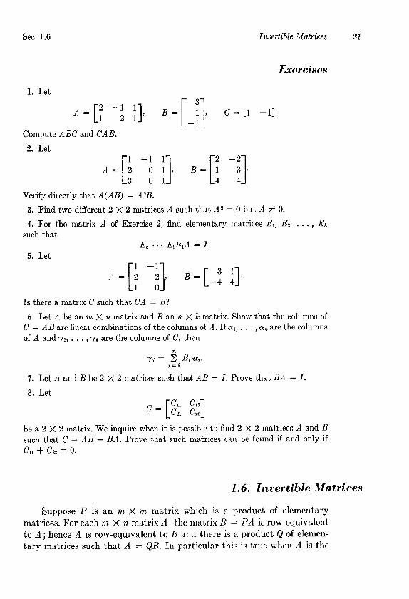
1. Let

A = [; -; ;I, B= [-J, c= r1 -11.

Compute ABC and CAB.

2. Let

A-[% -i ;], B=[; -;]a

Verify directly that A(AB) = A2B.

3. Find two different 2 X 2 matrices A such that A* = 0 but A # 0.

4. For the matrix A of Exercise 2, find elementary matrices El, Ez, . . . , Ek such that

Er ... EzElA = I.

5. Let

A=[i -;], B= [-I ;].

Is there a matrix C such that CA = B?

6. Let A be an m X n matrix and B an n X k matrix. Show that the columns of C = AB are linear combinations of the columns of A. If al, . . . , (Y* are the columns of A and yl, . . . , yk are the columns of C, then

yi = 2 B,g~p ?.=I

7. Let A and B be 2 X 2 matrices such that AB = 1. Prove that BA = I.

8. Let

be a 2 X 2 matrix. We inquire when it is possible to find 2 X 2 matrices A and B such that C = AB - BA. Prove that such matrices can be found if and only if Cl1 + czz = 0.

1.6. Invertible Matrices

Suppose P is an m X m matrix which is a product of elementary matrices. For each m X n matrix A, the matrix B = PA is row-equivalent to A; hence A is row-equivalent to B and there is a product Q of elementary matrices such that A = QB. In particular this is true when A is the


m X m identity matrix. In other words, there is an m X m matrix Q, which is itself a product of elementary matrices. such that QP = I. As we shall soon see, the existence of a Q with QP = I is equivalent to the fact that P is a product of elementary matrices.

DeJinition. Let A be an n X n (square) matrix over the field F. An n X n matrix B such that BA = I is called a left inverse of A; an n X n matrix B such that AB = I is called a right inverse of A. If AB = BA = I, then B is called a two-sided inverse of A and A is said to be invertible.

Lemma. Tf A has a left inverse B and a right inverse C, then B = C.

Proof. Suppose BA = I and AC = I. Then

B = BI = B(AC) = (BA)C = IC = C. 1

Thus if A has a left and a right inverse, A is invertible and has a unique two-sided inverse, which we shall denote by A-’ and simply call the inverse of A.

Theorem 10. Let A and B be n X n matrices over E’.

(i) If A is invertible, so is A-l and (A-l)-’ = A. (ii) If both A and B are invertible, so is AR, and (AB)-l = B-‘A-‘.

Proof. The first statement is evident from the symmetry of the definition. The second follows upon verification of the relations

(AB)(B-‘A-‘) = (B-‘A-‘)(AB) = I. 1

Corollary. A product of invertible matrices is invertible.

Theorem 11. An elementary matrix is invertible.

Proof. Let E be an elementary matrix corresponding to the elementary row operation e. If el is the inverse operation of e (Theorem 2) and El = el(1), then

and EE, = e(El) = e(el(I)) = I

ElE = cl(E) = el(e(I)) = I

so that E is invertible and E1 = E-l. 1

EXAMPLE 14.

(4

(b)


(cl [c’ ;I-l = [-: !I (d) When c # 0,

I

Theorem 12. If A is an n X n matrix, the following are equivalent.

(i) A is invertible. (ii) A is row-equivalent to the n X n identity matrix.

(iii) A is a product of elementary matrices.

Proof. Let R be a row-reduced echelon matrix which is row- equivalent to A. By Theorem 9 (or its corollary),

R = EI, . ’ . EzE,A

where El, . . . , Ee are elementary matrices. Each Ei is invertible, and so

A = EC’... E’,‘R.

Since products of invertible matrices are invertible, we see that A is invertible if and only if R is invertible. Since R is a (square) row-reduced echelon matrix, R is invertible if and only if each row of R contains a non-zero entry, that is, if and only if R = I. We have now shown that A is invertible if and only if R = I, and if R = I then A = EL’ . . . EC’. It should now be apparent that (i), (ii), and (iii) are equivalent statements about A. 1

Corollary. If A is an invertible n X n matrix and if a sequence of elementary row operations reduces A to the identity, then that same sequence of operations when applied to I yields A-‘.

Corollary. Let A and B be m X n matrices. Then B is row-equivalent to A if and only if B = PA where P is an invertible m X m matrix.

Theorem 13. For an n X n matrix A, the following are equivalent.

(i) A is invertible. (ii) The homogeneous system AX = 0 has only the trivial solution

x = 0. (iii) The system of equations AX = Y has a solution X for each n X 1

matrix Y.

Proof. According to Theorem 7, condition (ii) is equivalent to the fact that A is row-equivalent to the identity matrix. By Theorem 12, (i) and (ii) are therefore equivalent. If A is invertible, the solution of AX = Y is X = A-‘Y. Conversely, suppose AX = Y has a solution for each given Y. Let R be a row-reduced echelon matrix which is row-


equivalent to A. We wish to show that R = I. That amounts to showing that the last row of R is not (identically) 0. Let

0 0

Es i.

[I 0 1

If the system RX = E can be solved for X, the last row of R cannot be 0. We know that R = PA, where P is invertible. Thus RX = E if and only if AX = P-IE. According to (iii), the latter system has a solution. m

Corollary. A square matrix with either a left or right inverse is invertible.

Proof. Let A be an n X n matrix. Suppose A has a left inverse, i.e., a matrix B such that BA = I. Then AX = 0 has only the trivial solution, because X = IX = B(AX). Therefore A is invertible. On the other hand, suppose A has a right inverse, i.e., a matrix C such that AC = I. Then C has a left inverse and is therefore invertible. It then follows that A = 6-l and so A is invertible with inverse C. 1

Corollary. Let A = AlA, . . . Ak, where A1 . . . , Ak are n X n (square) matrices. Then A is invertible if and only if each Aj is invertible.

Proof. We have already shown that the product of two invertible matrices is invertible. From this one sees easily that if each Aj is invertible then A is invertible.

Suppose now that A is invertible. We first prove that Ak is invertible. Suppose X is an n X 1 matrix and AkX = 0. Then AX = (A1 ... Akel)AkX = 0. Since A is invertible we must have X = 0. The system of equations AkX = 0 thus has no non-trivial solution, so Ak is invertible. But now A1 . . . Ak--l = AAa’ is invertible. By the preceding argument, Ak-l is invertible. Continuing in this way, we conclude that each Aj is invertible. u

We should like to make one final comment about the solution of linear equations. Suppose A is an m X n matrix and we wish to solve the system of equations AX = Y. If R is a row-reduced echelon matrix which is row-equivalent to A, then R = PA where P is an m X m invertible matrix. The solutions of the system A& = Y are exactly the same as the solutions of the system RX = PY (= Z). In practice, it is not much more difficult to find the matrix P than it is to row-reduce A to R. For, suppose we form the augmented matrix A’ of the system AX = Y, with arbitrary scalars yl, . . . , ylnz occurring in the last column. If we then perform on A’ a sequence of elementary row operations which leads from A to R, it will


become evident what the matrix P is. (The reader should refer to Ex- ample 9 where we essentially carried out this process.) In particular, if A is a square matrix, this process will make it clear whether or not A is invertible and if A is invertible what the inverse P is. Since we have already given the nucleus of one example of such a computation, we shall content ourselves with a 2 X 2 example.

EXAMPLE 15. Suppose F is the field of rational numbers and

A= 2 -l [ 1 1 3’ Then

2 -1 y1 (3) 1 1 [ 3 yz (2) 1 3 y.2 (1) 1 3 yz - 2 71 y1 - 1 [ 0 -7 y1-2yz - 1

1 3 (2) 1 0 3(y2 + 3YI) 0 1 S(2yB2 y1) - 1 [ 0 1 4@Y, - Yl) 1

from which it is clear that A is invertible and

A-’ = + [ 1 + . -4 3 It may seem cumbersome to continue writing the arbitrary scalars

Yl, Y-2, . . . in the computation of inverses. Some people find it less awkward to carry along two sequences of matrices, one describing the reduction of A to the identity and the other recording the effect of the same sequence of operations starting from the identity. The reader may judge for him- self which is a neater form of bookkeeping.

EXAMPLE 16. Let us find the inverse of

0 0 1 1 0 0 1 1 0 0 1 1 0 0

180 1

Linear Equations Chap. 1 1 f 0

[ 1 0 1 09 001

10 0

[ I

0 1 07 00 1

--9 60

-36 192 -180 30 -180 -60 1 180 _

- 9 -36 30

-36 192 -180

I

. 30 -180 180

It must have occurred to the reader that we have carried on a lengthy discussion of the rows of matrices and have said little about the columns. We focused our attention on the rows because this seemed more natural from the point of view of linear equations. Since there is obviously nothing sacred about rows, the discussion in the last sections could have been carried on using columns rather than rows. If one defines an elementary column operation and column-equivalence in a manner analogous to that of elementary row operation and row-equivalence, it is clear that each m X n matrix will be column-equivalent to a ‘column-reduced echelon’ matrix. Also each elementary column operation will be of the form A + AE, where E is an n X n elementary matrix-and so on.

Exercises

1. Let

Find a row-reduced echelon matrix R which is row-equivalent to A and an invertible 3 X 3 matrix P such that R = PA.

2. Do Esercise 1, but with

A = [; -3 21.

3. For each of the two matrices

use elementary row operations to discover whether it is invertible, and to find the inverse in case it is.

4. Let 5 0

A= [ 15

0

0 1 0. 1 5


For which X does there exist a scalar c such that AX = cX?

5. Discover whether 1 2 3 4

A=O234 [ 1 0 0 3 4 0 0 0 4

is invertible, and find A-1 if it exists.

6. Suppose A is a 2 X I matrix and that B is a 1 X 2 matrix. Prove that C = AB is not invertible.

7. Let A be an n X n (square) matrix. Prove the following two statements: (a) If A is invertible and AB = 0 for some n X n matrix B, then B = 0. (b) If A is not invertible, then there exists an n X n matrix B such that

AB = 0 but B # 0.

8. Let

Prove, using elementary row operations, that A is invertible if and only if (ad - bc) # 0.

9. An n X n matrix A is called upper-triangular if Ai, = 0 for i > j, that is, if every entry below the main diagonal is 0. Prove that an upper-triangular (square) matrix is invertible if and only if every entry on its main diagonal is different from 0.

10. Prove the following generalization of Exercise 6. If A is an m X n matrix, B is an n X m matrix and n < m, then AB is not invertible.

11. Let A be an m X n matrix. Show that by means of a finite number of elementary row and/or column operations one can pass from A to a matrix R which is both ‘row-reduced echelon’ and ‘column-reduced echelon,’ i.e., Rii = 0 if i # j,

Rii = 1, 1 5 i 5 r, Rii = 0 if i > r. Show that R = PA&, where P is an invertible m X m matrix and Q is an invertible n X n matrix.

12. The result of Example 16 suggests that perhaps the matrix

is invertible and A+ has integer entries. Can you prove that?

40 Vector Spaces Chap. 2

5. Let I” be a field and let 12 be a positive integer (n 2 2). Let V be the vector space of all n X n matrices over Ii’. Which of the following sets of matrices B in V are subspaces of V?

(a) all invertible A ; (b) all non-invertible A ; (c) all A such that AB = &I, where B is some fixed matrix in V; (d) all A such that A2 = A.

6. (a) Prove that the only subspaces of R1 are R1 and the zero subspace. (b) Prove that a subspace of R* is R2, or the zero subspace, or consists of all

scalar multiples of some fixed vector in R2. (The last type of subspace is, intuitively, a straight line through the origin.)

(c) Can you describe the subspaces of R3?

7. Let WI and WZ be subspaces of a vector space V such that the set-theoretic union of WI and Wz is also a subspace. Prove that one of the spaces Wi is contained in the other.

8. Let 7.7 be the vector space of all functions from R into R; let 8, be the subset of even functions, f(-2) = f(s); let V, be the subset of odd functions,

f(-z) = -f(z).

(a) Prove that 8, and V, are subspaces of V. (b) Prove that V, + V, = V. (c) Prove that V, n V, = (0).

9. Let WI and Wz be subspaces of a vector space V such that WI + Wz = V and WI n W2 = (0). Prove that for each vector LY in V there are unique vectors (Ye in WI and (Ye in W2 such that a = crI + LYE.

2.3. Bases and Dimension

We turn now to the task of assigning a dimension to certain vector

spaces. Although we usually associate ‘dimension’ with something geomet-

rical, we must find a suitable algebraic definition of the dimension of a

vector space. This will be done through the concept of a basis for the space.

DeJinition. Let V be a vector space over F. A subset S of TJ is said to

be linearly dependent (or simply, dependent) if there exist distinct vectors

a, a-2, . . . ) (Y,, in S and scalars cl, c2, . . . , c, in F, not all of which are 0,

such that

Clcrl + c.gY2 + . * - + C&t, = 0.

A set which is not linearly dependent is called linearly independent. If the set S contains only$nitely many vectors q, o(~, . . . , LY,, we sometimes say that cq, a2, . . . , 01, are dependent (or independent) instead of saying S is

dependent (or independent) .

Sec. 2.3 Bases and Dimension

The following are easy consequences of the definition.

1. Any set which contains a linearly dependent set is linearly dependent.

41

2. Any subset of a linearly independent set is linearly independent. 3. Any set which contains the 0 vector is linearly dependent; for

1 * 0 = 0. 4. A set X of vectors is linearly independent if and only if each finite

subset of S is linearly independent, i.e., if and only if for any distinct vectors cq, . . . , a, of X, clczl + . . . + c,(Y, = 0 implies each ci = 0.

Definition. Let V be a vector space. A basis for V is a lineady inde-

pendent set of vectors in V ‘which spans the space V. The space V is finite-

dimensional if it has aJinite basis.

EXAMPLE 12. Let F be a subfield of the complex numbers. In F3 the vectors

w=( 3,0,-3)

a2 = (-1, 1, 2) a3 = ( 4, 2, -2)

a4 = ( 2, 1, 1)

are linearly dependent, since

201 + 2cYz - cY3 + 0 . a4 = 0. The vectors

El = 0, 0, 0) E2 = (0, 1, 0) E3 = (0, 0, 1)

are linearly independent

EXAMPLE 13. Let F be a field and in Fn let S be the subset consisting of the vectors cl, c2, . . . , G, defined by

t1 = (1, 0, 0, . . . , 0) c2 = (0, 1, 0, . . . ) 0)

. . . . . . .

tn = (0, 0, 0, . . . ) 1).

Let x1, x2, . . . , xn be scalars in F and put (Y = xlcl + x2c2 + . . . + x,E~. Then

(2-12) a= (x1,52 )...) 5,).

This shows that tl, . . . , E, span Fn. Since a! = 0 if and only if x1 = x2 = . . . = 5, = 0, the vectors Q, . . . , E~ are linearly independent. The set S = {q, . . . , en} is accordingly a basis for Fn. We shall call this particular basis the standard basis of P.

Vector Spaces Chap. 2

EXAMPLE 14. Let P be an invertible n X n matrix with entries in the field F. Then PI, . . . , P,, the columns of P, form a basis for the space of column matrices, FnX1. We see that as follows. If X is a column matrix, then

PX = XlPl + . . * + xnPn.

Since PX = 0 has only the trivial solution X = 0, it follows that {Pl, . . . , P,} is a linearly independent set. Why does it span FnX1? Let Y be any column matrix. If X = P-‘Y, then Y = PX, that is,

Y = XlPl + * ’ * + G&P,.

so (Pl, . . . , Pn) is a basis for Fnxl.

EXAMPLE 15. Let A be an m X n matrix and let S be the solution space for the homogeneous system AX = 0 (Example 7). Let R be a row- reduced echelon matrix which is row-equivalent to A. Then S is also the solution space for the system RX = 0. If R has r non-zero rows, then the system of equations RX = 0 simply expresses r of the unknowns x1, . . . , xn in terms of the remaining (n - r) unknowns xi. Suppose that the leading non-zero entries of the non-zero rows occur in columns kl, . . . , k,. Let J be the set consisting of the n - r indices different from kl, . . . , k,:

J = (1, . . . , n} - {kl, . . . , IGT}.

The system RX = 0 has the form

xk, i- i? cljxj = 0 J

xk, + Z G$j = 0 J

where the cij are certain scalars. All solutions are obtained by assigning (arbitrary) values to those xj’s with j in J and computing the corresponding values of xk,, . . . , %k,. For each j in J, let Ei be the solution obtained by setting xj = 1 and xi = 0 for all other i in J. We assert that the (n - r) vectors Ej, j in J, form a basis for the solution space.

Since the column matrix Ej has a 1 in row j and zeros in the rows indexed by other elements of J, the reasoning of Example 13 shows us that the set of these vectors is linearly independent. That set spans the solution space, for this reason. If the column matrix T, with entries t1, . . . , t,, is in the solution space, the matrix

N = 2; tjEj J

is also in the solution space and is a solution such that xi = tj for each j in J. The solution with that property is unique; hence, N = T and T is in the span of the vectors Ej.

Sec. 2.3 Bases and Dimension 43

EXAMPLE 16. We shall now give an example of an infinite basis. Let F be a subfield of the complex numbers and let I’ be the space of polynomial functions over F. Recall that these functions are the functions from F into F which have a rule of the form

f(x) = co + ClX + * . . + c,xn.

Let 5(z) = xk, Ic = 0, 1, 2, . . . . The (infinite) set {fo, fr, fi, . . .} is a basis for V. Clearly the set spans V, because the functionf (above) is

f = cofo + Clfl + * * * + cnfn.

The reader should see that this is virtually a repetition of the definition of polynomial function, that is, a function f from F into F is a polynomial function if and only if there exists an integer n and scalars co, . . . , c, such that f = cofo + . . . + cnfn. Why are the functions independent? To show that the set {fo, h, .h, . . .} is independent means to show that each finite subset of it is independent. It will suffice to show that, for each n, the set dfo, * * * , fn) is independent. Suppose that

Cojfo + * * * + cJn = 0.

This says that co + ClX + * * * + cnxn = 0

for every x in F; in other words, every x in F is a root of the polynomial f(x) = co + ClX + * . . + cnxn. We assume that the reader knows that a polynomial of degree n with complex coefficients cannot have more than n distinct roots. It follows that co = cl = . . . = c, = 0.

We have exhibited an infinite basis for V. Does that mean that V is not finite-dimensional? As a matter of fact it does; however, that is not immediate from the definition, because for all we know V might also have a finite basis. That possibility is easily eliminated. (We shall eliminate it in general in the next theorem.) Suppose that we have a finite number of polynomial functions gl, . . . , gT. There will be a largest power of z which appears (with non-zero coefficient) in gl(s), . . . , gJx). If that power is Ic, clearly fk+l(x) = xk+’ is not in the linear span of 91, . . . , g7. So V is not finite-dimensional.

A final remark about this example is in order. Infinite bases have nothing to do with ‘infinite linear combinations.’ The reader who feels an irresistible urge to inject power series

co z CkXk

k=O

into this example should study the example carefully again. If that does not effect a cure, he should consider restricting his attention to finite- dimensional spaces from now on.


Theorem 4. Let V be a vector space which is spanned by a finite set of vectors PI, & . . . , Pm. Then any independent set of vectors in V is jinite and contains no more than m elements.

Proof. To prove the theorem it suffices to show that every subset X of V which contains more than m vectors is linearly dependent. Let S be such a set. In S there are distinct vectors (~1, Q, . . . , (Y, where n > m. Since pl, . . . , Pm span V, there exist scalars Aij in F such that

For any n scalars x1, x2, . . . , x, we have

XlLyl + . . . + XfS(r?l = i XjcUj j=l

Since n > m, Theorem 6 of Chapter 1 implies that there exist scalars a, x2, . . . , xn not all 0 such that

5 Aijxj=O, l<i<m. j=l

Hence xlal + x2a2 + + . . + X~CG, = 0. This shows that S is a linearly dependent set. 1

Corollary 1. If V is a finite-dimensional vector space, then any two bases of V have the same (jinite) number of elements.

Proof. Since V is finite-dimensional, it has a finite basis

@l,PZ,. . .,Pm).

By Theorem 4 every basis of V is finite and contains no more than m elements. Thus if {CQ, +, . . . , oc,} is a basis, n I m. By the same argument, m 2 n. Hence m = n. 1

This corollary allows us to define the dimension of a finite-dimensional vector space as the number of elements in a basis for V. We shall denote the dimension of a finite-dimensional space V by dim V. This allows us to reformulate Theorem 4 as follows.

Corollary 2. Let V be a finite-dimensional vector space and let n = dim V. Then

Sec. 2.3 Bases and Dimension 45

(a) any subset of V which contains more than n vectors is linearly dependent;

(b) no subset of V which contains fewer than n vectors can span V.

EXAMPLE 17. If F is a field, the dimension of Fn is n, because the standard basis for Fn contains n vectors. The matrix space Fmxlr has dimension mn. That should be clear by analogy with the case of Fn, because the mn matrices which have a 1 in the i, j place with zeros elsewhere form a basis for Fmxn. If A is an m X n matrix, then the solution space for A has dimension n - r, where r is !he number of non-zero rows in a row-reduced echelon matrix which is row-equivalent to A. See Example 15.

If V is any vector space over F, the zero subspace of V is spanned by the vector 0, but {0} is a linearly dependent set and not a basis. For this reason, we shall agree that the zero subspace has dimension 0. Alterna- tively, we could reach the same conclusion by arguing that the empty set is a basis for the zero subspace. The empty set spans {0}, because the intersection of all subspaces containing the empty set is {0}, and the empty set is linearly independent because it contains no vectors.

Lemma. Let S be a linearly independent subset of a vector space V. Suppose p is a vector in V which is not in the subspace spanned by S. Then the set obtained by adjoining p to S is linearly independent.

Proof. Suppose al, . . . , CY, are distinct vectors in S and that

Clcrl + * * - + ~,,,a, + bfi = 0.

Then b = 0; for otherwise,

p= -; al+... ( >

+ -2 ffm ( >

and fi is in the subspace spanned by S. Thus clal + . . . + cn,ol, = 0, and since S is a linearly independent set each ci = 0. 1

Theorem 5. If W is a subspace of a finite-dimensional vector space V, every linearly independent subset of W is finite and is part of a (finite) basis for W.

Proof. Suppose So is a linearly independent subset of W. If X is a ‘inearly independent subset of W containing So, then S is also a linearly independent subset of V; since V is finite-dimensional, S contains no more than dim V elements.

We extend So to a basis for W, as follows. If So spans W, then So is a basis for W and we are done. If So does not span W, we use the preceding lemma to find a vector p1 in W such that the set S1 = 2%~ U {PI} is independent. If S1 spans W, fine. If not, npolv the lemma to obtain a vector 02


in W such that Sz = X1 U {/3z> is independent. If we continue in this way, then (in not more than dim V steps) we reach a set

s, = so u {Pl, f . . , PnJ

which is a basis for W. 1

Corollary 1. Ij W is a proper subspace of a finite-dimensional vector space V, then W is finite-dimensional and dim W < dim V.

Proof. We may suppose W contains a vector cy # 0. By Theorem 5 and its proof, there is a basis of W containing (Y which contains no more than dim V elements. Hence W is finite-dimensional, and dim W 5 dim V. Since W is a proper subspace, there is a vector /3 in V which is not in W. Adjoining p to any basis of W, we obtain a linearly independent subset of V. Thus dim W < dim V. 1

Corollary 2. In a finite-dimensional vector space V every non-empty linearly independent set of vectors is part of a basis.

Corollary 3. Let A be an n X n matrix over a field F, and suppose the row vectors of A form a linearly independent set of vectors in F”. Then A is invertible.

Proof. Let (~1, crz, . . . , ayn be the row vectors of A, and suppose W is the subspace of Fn spanned by al, (Ye, . . . , czn. Since al, LYE, . . . , (Ye are linearly independent, the dimension of W is n. Corollary 1 now shows that W = F”. Hence there exist scalars Bij in F such that

E; = i B.. G3) lliln j=l

where (~1, Q, . . . , en} is the standard basis of Fn. Thus for the matrix B with entries Bii we have

BA = I. 1

Theorem 6. If WI and Wz are finite-dimensional subspaces of a vector space V, then Wr + Wz is Jinite-dimensional and

dim Wr + dim Wz = dim (WI n W,) + dim (WI + WZ).

Proof. By Theorem 5 and its corollaries, W1 n W2 has a finite basis {cq, . . . , CQ} which is part of a basis

{al, . . . , Uk, Pl, * * . , Pm) for WI

and part of a basis

1 al, . . . , ak, -t’l, . . . , rn} for Wz.

The subspace Wl + W2 is spanned by the vectors

Sec. 2.3 Bases and Dimension

and these vectors form an independent set. For suppose

Z XiO!i + 2 yjfij + Z 277~ = 0. Then

- 2 7$-y, = 2 Xi% + L: YjPj

which shows that Z z,y, belongs to W,. As 2 x,y, also belongs to W, it follows that

2 X,y, = 2 CiCti

for certain scalars cl, . . . , ck. Because the set

{ al) . . . , ax, Yl, . . . , Yn >

is independent, each of the scalars X~ = 0. Thus

2 XjOri + Z yjpj = 0 and since

{% . . . , ak, 01, . . . , &)

is also an independent set, each zi = 0 and each y, = 0. Thus,

{ al, . . . , ak, Pl, . . . , bn, 71, . . . , -in >

is a basis for WI + Wz. Finally

dim WI + dim l,t7, = (Ic + m) + (Ic + n) =k+(m+k+n) = dim (W, n Wz) + dim (WI + W,). 1

Let us close this section with a remark about linear independence and dependence. We defined these concepts for sets of vectors. It is useful to have them defined for finite sequences (ordered n-tuples) of vectors: al, . . . ) a,. We say that the vectors (~1, . . . ,01, are linearly dependent

if there exist scalars cl, . . . , c,, not all 0, such that clczl + . . . + cnan = 0. This is all so natural that the reader may find that he has been using this terminology already. What is the difference between a finite sequence al. . . ,&I and a set {CQ, . . . , CY,}? There are two differences, identity and order.

If we discuss the set {(Ye, . . . , (Y,}, usually it is presumed that no two of the vectors CQ . . . , 01, are identical. In a sequence CQ, . . . , ac, all the CX;)S may be the same vector. If ai = LYE for some i # j, then the sequence (Y], . . . , 01, is linearly dependent:

(Yi + (-1)CXj = 0.

Thus, if CY~, . . . , LYE are linearly independent, they are distinct and we may talk about the set {LYE, . . . , a,} and know that it has n vectors in it. So, clearly, no confusion will arise in discussing bases and dimension. The dimension of a finite-dimensional space V is the largest n such that some n-tuple of vectors in V is linearly independent-and so on. The reader

Vector Spaces Chap. 2

who feels that this paragraph is much ado about nothing might ask him-

self whether the vectors

a1 = (esj2, 1)

a2 = (rn, 1)

are linearly independent in Rx.

The elements of a sequence are enumerated in a specific order. A set

is a collection of objects, with no specified arrangement or order. Of

course, to describe the set we may list its members, and that requires

choosing an order. But, the order is not part of the set. The sets {1,2, 3,4}

and (4, 3, 2, l} are identical, whereas 1, 2,3,4 is quite a different sequence

from 4, 3, 2, 1. The order aspect of sequences has no bearing on ques-

tions of independence, dependence, etc., because dependence (as defined)

is not affected by t,he order. The sequence o(,, . . . , o(] is dependent if and

only if the sequence al, . . . , 01, is dependent. In the next section, order

will be important.

Exercises

1. Prove that if two vectors are linearly dependent, one of them is a scalar multiple of the other.

2. Are the vectors

a1 = (1, 1, 2,4), cY2 = (2, -1, -5, 2)

a.3 = (1, -1, -4,O), a4 = (2, 1, 1, 6)

linearly independent in R4?

3. Find a basis for the subspace of R4 spanned by the four vectors of Exercise 2.

4. Show that the vectors

a = (1, 0, --I), ffz = (1, 2, I), a3 = (0, -3, 2)

form a basis for R3. Express each of the standard basis vectors as linear combinations of al, (Ye, and LYE.

5. Find three vectors in R3 which are linearly dependent, and are such that any two of them are linearly independent.

6. Let V be the vector space of all 2 X 2 matrices over the field F. Prove that V has dimension 4 by exhibiting a basis for V which has four elements,

7. Let V be the vector space of Exercise 6. Let W1 be the set of matrices of the form

X -x 1 1 Y 2 and let Wz be the set of matrices of the form

Documents

LINEAR ALGEBRA - oms.bdu.ac.in