Embed Size (px)
Citation preview

Linear Algebra
Joseph R. Mileti
April 3, 2019

2
Contents
1 Introduction 51.1 What is Linear Algebra? . . . . . . . . . . . . . . . . . . . . . . . . . . . . . . . . . . . . . . . 51.2 Mathematical Statements and Mathematical Truth . . . . . . . . . . . . . . . . . . . . . . . . 101.3 Quantifiers and Proofs . . . . . . . . . . . . . . . . . . . . . . . . . . . . . . . . . . . . . . . . 141.4 Evens and Odds . . . . . . . . . . . . . . . . . . . . . . . . . . . . . . . . . . . . . . . . . . . 241.5 Sets, Set Construction, and Subsets . . . . . . . . . . . . . . . . . . . . . . . . . . . . . . . . . 311.6 Functions . . . . . . . . . . . . . . . . . . . . . . . . . . . . . . . . . . . . . . . . . . . . . . . 371.7 Injective, Surjective, and Bijective Functions . . . . . . . . . . . . . . . . . . . . . . . . . . . 441.8 Solving Equations . . . . . . . . . . . . . . . . . . . . . . . . . . . . . . . . . . . . . . . . . . 48
2 Spans and Linear Transformations in Two Dimensions 512.1 Intersections of Lines in R2 . . . . . . . . . . . . . . . . . . . . . . . . . . . . . . . . . . . . . 512.2 Vectors in R2 . . . . . . . . . . . . . . . . . . . . . . . . . . . . . . . . . . . . . . . . . . . . . 542.3 Spans . . . . . . . . . . . . . . . . . . . . . . . . . . . . . . . . . . . . . . . . . . . . . . . . . 562.4 Linear Transformations of R2 . . . . . . . . . . . . . . . . . . . . . . . . . . . . . . . . . . . . 682.5 The Standard Matrix of a Linear Transformation . . . . . . . . . . . . . . . . . . . . . . . . . 822.6 Matrix Algebra . . . . . . . . . . . . . . . . . . . . . . . . . . . . . . . . . . . . . . . . . . . . 922.7 Range, Null Space, and Inverses . . . . . . . . . . . . . . . . . . . . . . . . . . . . . . . . . . . 102
3 Coordinates and Eigenvectors in Two Dimensions 1173.1 Coordinates and Change of Basis . . . . . . . . . . . . . . . . . . . . . . . . . . . . . . . . . . 1173.2 Matrices with Respect to Other Coordinates . . . . . . . . . . . . . . . . . . . . . . . . . . . . 1243.3 Eigenvalues and Eigenvectors . . . . . . . . . . . . . . . . . . . . . . . . . . . . . . . . . . . . 1343.4 Determinants . . . . . . . . . . . . . . . . . . . . . . . . . . . . . . . . . . . . . . . . . . . . . 152
4 Beyond Two Dimensions 1594.1 Vector Spaces and Subspaces . . . . . . . . . . . . . . . . . . . . . . . . . . . . . . . . . . . . 1594.2 Solving Linear Systems . . . . . . . . . . . . . . . . . . . . . . . . . . . . . . . . . . . . . . . . 171
3

4 CONTENTS
Chapter 1
Introduction
1.1 What is Linear Algebra?
The most elementary, yet honest, way to describe linear algebra is that it is the basic mathematics of highdimensions. By “basic”, we do not mean that the theory is easy, but only that it is essential to a morenuanced understanding of the mathematics of high dimensions. For example, the simplest curves in twodimensions are lines, and we use lines to approximate more complicated curves in Calculus. Similarly, themost basic surfaces in three dimensions are planes, and we use planes to approximate more complicatedsurfaces. One of our major goals will be to generalize the concepts of lines and planes to the “flat” objects inhigh dimensions. Another major goal will be to understand the simplest kinds of functions (so-called lineartransformations) that arise in this setting. If this sounds abstract and irrelevant to real world problems,we will explain in the rest of this section, and throughout the course, why these concepts are incrediblyimportant to mathematics and its applications.
Generalizing Lines and Planes
Let’s begin by recalling how we can describe a line in two dimensions. One often thinks about a line asthe solution set to an equation of the form y = mx + b (where m and b are fixed numbers). Althoughmost lines in two dimensions can arise from such equations, these descriptions omit vertical lines. A better,more symmetric, and universal way to describe a line is as the set of solutions to an equation of the formax+ by = c, where at least one of a or b is nonzero. For example, we can now describe the vertical line x = 5using the numbers a = 1, b = 0, and c = 5. Notice that if b is nonzero, then we can equivalently write thisequation as y = (−ab )x+ c
b , which fits into the above model. Similarly, if a is nonzero, then we can solve forx in terms of y.
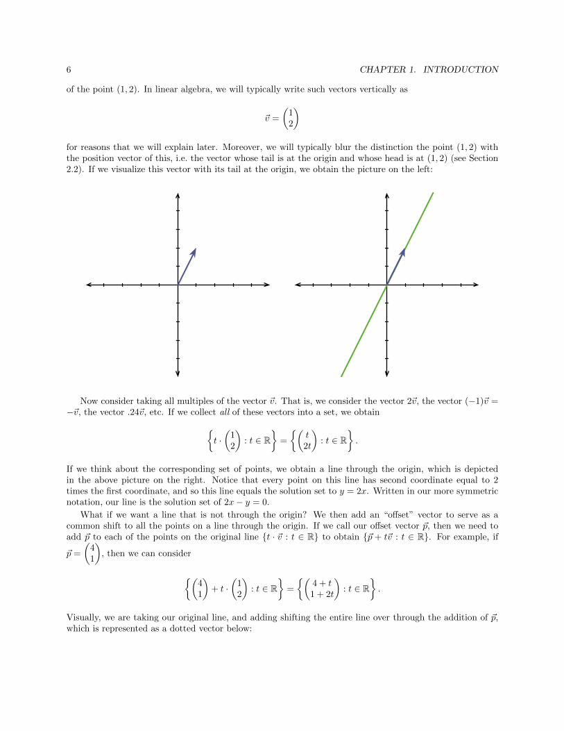
With this approach, we are thinking about a line as described algebraically by an equation. However,there is another, more geometric, way to describe a line in two dimensions. Start with a nonzero vector ~v inthe plane R2 (with its tail at the origin), and think about taking the collection of all scalar multiples of ~v. Inother words, stretch the vector ~v in all possible ways, including switching its direction around using negativescalars, and consider all possible outcomes. In set-theoretic notation, we are forming the set {t · ~v : t ∈ R}(if this symbolism is unfamiliar to you, we will discuss set-theoretic notation in detail later). When viewedas a collection of points, this set consists of a line through the origin in the direction of ~v.
For example, consider the vector ~v in the plane whose first coordinate is 1 and whose second coordinateis 2. In past courses, you may have written ~v as the vector 〈1, 2〉, and thought about it as the position vector
5
6 CHAPTER 1. INTRODUCTION
of the point (1, 2). In linear algebra, we will typically write such vectors vertically as
~v =
(12
)for reasons that we will explain later. Moreover, we will typically blur the distinction the point (1, 2) withthe position vector of this, i.e. the vector whose tail is at the origin and whose head is at (1, 2) (see Section2.2). If we visualize this vector with its tail at the origin, we obtain the picture on the left:
Now consider taking all multiples of the vector ~v. That is, we consider the vector 2~v, the vector (−1)~v =−~v, the vector .24~v, etc. If we collect all of these vectors into a set, we obtain{
t ·(
12
): t ∈ R
}=
{(t2t
): t ∈ R
}.
If we think about the corresponding set of points, we obtain a line through the origin, which is depictedin the above picture on the right. Notice that every point on this line has second coordinate equal to 2times the first coordinate, and so this line equals the solution set to y = 2x. Written in our more symmetricnotation, our line is the solution set of 2x− y = 0.
What if we want a line that is not through the origin? We then add an “offset” vector to serve as acommon shift to all the points on a line through the origin. If we call our offset vector ~p, then we need toadd ~p to each of the points on the original line {t · ~v : t ∈ R} to obtain {~p + t~v : t ∈ R}. For example, if
~p =
(41
), then we can consider
{(41
)+ t ·
(12
): t ∈ R
}=
{(4 + t1 + 2t
): t ∈ R
}.
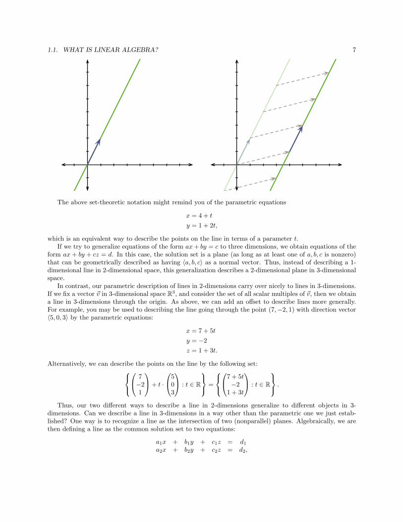
Visually, we are taking our original line, and adding shifting the entire line over through the addition of ~p,which is represented as a dotted vector below:
1.1. WHAT IS LINEAR ALGEBRA? 7
The above set-theoretic notation might remind you of the parametric equations
x = 4 + t
y = 1 + 2t,
which is an equivalent way to describe the points on the line in terms of a parameter t.If we try to generalize equations of the form ax+ by = c to three dimensions, we obtain equations of the
form ax + by + cz = d. In this case, the solution set is a plane (as long as at least one of a, b, c is nonzero)that can be geometrically described as having 〈a, b, c〉 as a normal vector. Thus, instead of describing a 1-dimensional line in 2-dimensional space, this generalization describes a 2-dimensional plane in 3-dimensionalspace.
In contrast, our parametric description of lines in 2-dimensions carry over nicely to lines in 3-dimensions.If we fix a vector ~v in 3-dimensional space R3, and consider the set of all scalar multiples of ~v, then we obtaina line in 3-dimensions through the origin. As above, we can add an offset to describe lines more generally.For example, you may be used to describing the line going through the point (7,−2, 1) with direction vector〈5, 0, 3〉 by the parametric equations:
x = 7 + 5t
y = −2
z = 1 + 3t.
Alternatively, we can describe the points on the line by the following set: 7−21
+ t ·
503
: t ∈ R
=
7 + 5t−2
1 + 3t
: t ∈ R
.
Thus, our two different ways to describe a line in 2-dimensions generalize to different objects in 3-dimensions. Can we describe a line in 3-dimensions in a way other than the parametric one we just estab-lished? One way is to recognize a line as the intersection of two (nonparallel) planes. Algebraically, we arethen defining a line as the common solution set to two equations:
a1x + b1y + c1z = d1a2x + b2y + c2z = d2,
8 CHAPTER 1. INTRODUCTION
with appropriate conditions that enforce that the planes are not parallel.
Can we also describe a plane parametrically? Consider an arbitrary plane in R3 through the origin.Think about taking two nonzero and nonparallel vectors ~u and ~w parallel to the plane, and then using themto “sweep out” the rest of the plane. In other words, we want to focus on ~u and ~w, and then stretch and addthem in all possible ways to “fill in” the remaining points, similar to how we filled in points in 2-dimensionsby just stretching one vector. In set-theoretic notation, we are considering the set {t~u+ s~w : t, s ∈ R}. Forexample, if
~u =
2−31
and ~w =
−714
,
then we have the set t · 2−31
+ s ·
−714
: t, s ∈ R
=
2t− 7s−3t+ st+ 4s
: t, s ∈ R
.
This idea of combining vectors in all possible ways through scaling and adding will be a fundamental toolfor us. As above, if we want to think about planes in general (not just through the origin), then we shouldadd an offset.
With all of this in mind, can we generalize the ideas of lines and planes to higher dimensions? Whatwould be the analogue of a plane in 4-dimensions? How can we describe a 3-dimensional “flat” object (likea line or a plane) in 7-dimensions? Although these are fascinating pure mathematics questions, you maywonder why we would care.
In calculus, you learned how to compute projections in R2 and R3 based on the dot product (such ashow to project one vector onto another, or how to project a point onto a plane). One of our goals will beto generalize the ideas behind dot products and projections to higher dimensions. An important situationwhere this arises in practice is how to fit the “best” possible curve to some data points. For instance,suppose that we have n data points and want to fit the “best” line, parabola, etc. to these points. Wewill define “best” by saying that it minimizes a certain “distance”, defined in terms of our generalized dotproduct (this is analogous to the fact that the projection of a point onto a plane minimizes the distancebetween the given point and the projected point). By viewing the collection of all possible lines as a certain2-dimensional object inside of Rn, we will see that we can take a similar approach in Rn. Hence, fitting aline to n points can be thought of as projecting onto a certain “generalized plane” in Rn. Similarly, fittinga parabola amounts to projecting a point in Rn onto a 3-dimensional object. These examples demonstratethe power of that arises from understanding high dimensions. Moreover, these ideas lie at the heart of manyother applications, such as filling in missing data in order to reconstruct parts of an image that have beenlost, or predicting which movies you might like on Netflix in order to provide recommendations.
Transformations of Space
In Calculus, you studied functions f : R → R where both the input and output are elements of R. InMultivariable Calculus, you looked at functions f : R→ Rn (where the inputs are numbers and the outputsare elements of n-dimensional space) which can be thought of as parametric descriptions of curves in Rn. Forexample, the function f : R→ R2 given by f(t) = (cos t, sin t) can be viewed as a parametric description ofthe unit circle. After that, you investigated functions f : Rn → R where, for instance, the graph of a functionf : R2 → R like f(x, y) = x2 + y2 can be visualized as a surface in R3. Perhaps at the end of MultivariableCalculus you started to think about functions f : Rm → Rn. For example, consider the function f : R2 → R2
given by
f(x, y) = (x− y, x+ y).
1.1. WHAT IS LINEAR ALGEBRA? 9
In our new notation where we write vectors vertically, we could write this function as follows:
f
((xy
))=
(x− yx+ y
).
Notice that we have double parentheses on the left because we are thinking of the vector
(xy
)as one input
to the function f . For example, we have
f
((10
))=
(11
), f
((11
))=
(02
), and f
((01
))=
(−11
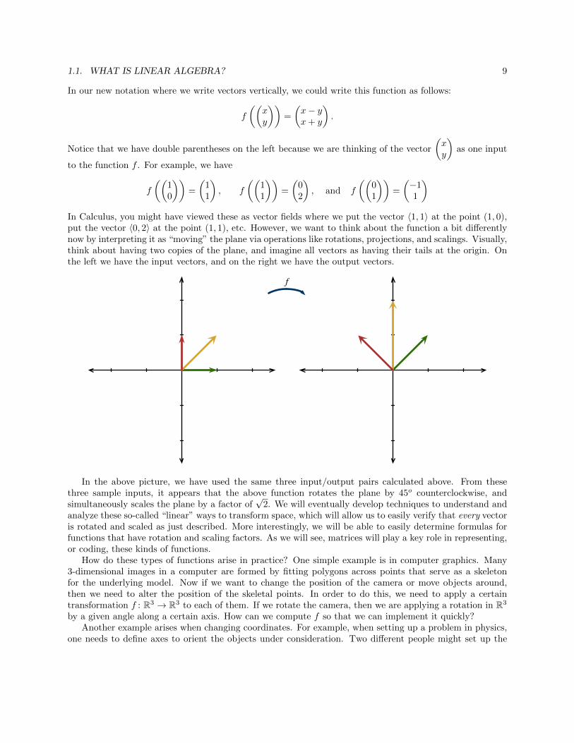
)In Calculus, you might have viewed these as vector fields where we put the vector 〈1, 1〉 at the point (1, 0),put the vector 〈0, 2〉 at the point (1, 1), etc. However, we want to think about the function a bit differentlynow by interpreting it as “moving” the plane via operations like rotations, projections, and scalings. Visually,think about having two copies of the plane, and imagine all vectors as having their tails at the origin. Onthe left we have the input vectors, and on the right we have the output vectors.
f
In the above picture, we have used the same three input/output pairs calculated above. From thesethree sample inputs, it appears that the above function rotates the plane by 45o counterclockwise, andsimultaneously scales the plane by a factor of
√2. We will eventually develop techniques to understand and
analyze these so-called “linear” ways to transform space, which will allow us to easily verify that every vectoris rotated and scaled as just described. More interestingly, we will be able to easily determine formulas forfunctions that have rotation and scaling factors. As we will see, matrices will play a key role in representing,or coding, these kinds of functions.
How do these types of functions arise in practice? One simple example is in computer graphics. Many3-dimensional images in a computer are formed by fitting polygons across points that serve as a skeletonfor the underlying model. Now if we want to change the position of the camera or move objects around,then we need to alter the position of the skeletal points. In order to do this, we need to apply a certaintransformation f : R3 → R3 to each of them. If we rotate the camera, then we are applying a rotation in R3
by a given angle along a certain axis. How can we compute f so that we can implement it quickly?Another example arises when changing coordinates. For example, when setting up a problem in physics,
one needs to define axes to orient the objects under consideration. Two different people might set up the
10 CHAPTER 1. INTRODUCTION
axes differently, and hence might use different coordinates for the position of a given object. I might label anobject by the coordinates (3, 1,−8) in my system, while you label it as (−2, 5, 0) in your system. We wouldlike to have a way to translate between our different ways of measuring, and it turns out that we can do thisby a “linear” transformation (sometimes with an offset similar to that used in our lines and planes) from R3
to R3. Working out how to do this is not only important for calculations, but is essential in understandingthe invariance of physical laws under certain changes of coordinates.
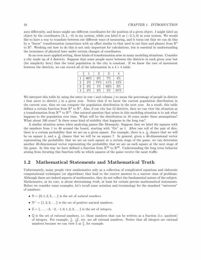
In an even more applied setting, these kinds of transformation arise in many modeling situations. Considera city made up of 4 districts. Suppose that some people move between the districts in each given year but(for simplicity here) that the total population in the city is constant. If we know the rate of movementbetween the districts, we can record all of the information in a 4× 4 table:
1 2 3 4
1 86% 3% 7% 4%2 2% 75% 11% 12%3 3% 1% 93% 3%4 2% 2% 5% 91%
We interpret this table by using the entry in row i and column j to mean the percentage of people in districti that move to district j in a given year. Notice that if we know the current population distribution inthe current year, then we can compute the population distribution in the next year. As a result, this tabledefines a certain function from R4 to R4. Also, if our city has 12 districts, then we can view the situation asa transformation from R12 to R12. One natural question that arises in this modeling situation is to ask whathappens to the population over time. What will be the distribution in 10 years under these assumptions?What about 100 years? Is there some kind of stability that happens in the long run?
A similar situation arises when analyzing games like Monopoly. Suppose that we label the squares withthe numbers from 1 to 40 around the board, starting with “Go” as 1. After one roll of the pair of dice,there is a certain probability that we are on a given square. For example, there is a 1
18 chance that we willbe on square 4, and a 5
36 chance that we will be on square 7. In general, given a 40-dimensional vectorrepresenting the probability that we are on each square at a certain stage of the game, we can determineanother 40-dimensional vector representing the probability that we are on each square at the next stage ofthe game. In this way we have defined a function from R40 to R40. Understanding the long term behaviorarising from iterating this function tells us which squares of the game receive the most traffic.
1.2 Mathematical Statements and Mathematical Truth
Unfortunately, many people view mathematics only as a collection of complicated equations and elaboratecomputational techniques (or algorithms) that lead to the correct answers to a narrow class of problems.Although these are indeed aspects of mathematics, they do not reflect the fundamental nature of the subject.Mathematics, at its core, is about determining truth, at least for certain precise mathematical statements.Before we consider some examples, let’s recall some notation and terminology for the standard “universes”of numbers:
• N = {0, 1, 2, 3, . . . } is the set of natural numbers.
• N+ = {1, 2, 3, . . . } is the set of positive natural numbers.
• Z = {. . . ,−3,−2,−1, 0, 1, 2, 3, . . . } is the set of integers.
• Q is the set of rational numbers, i.e. those numbers that can be written as a fraction (i.e. quotient)of integers. For example, 1
2 , −317 , etc. are all rational numbers. Notice that all integers are rationalnumbers because we can view 5 as 5
1 , for example.
1.2. MATHEMATICAL STATEMENTS AND MATHEMATICAL TRUTH 11
• R is the set of real numbers, i.e. those numbers that we can express as a (possibly infinite) decimal.Every rational number is a real number, but π, e,
√2, etc. are all real numbers that are not rational.
There are other important universes of numbers, such as the complex numbers C, and many more that youwill encounter in Abstract Algebra. However, we will focus on the above examples in our study. To denotethat a given number n belongs to one of the above collections, we will use the ∈ symbol. For example, wewill write n ∈ Z as shorthand for “n is an integer”. We will elaborate on how to use the symbol ∈ morebroadly when we discuss general set theory notation.
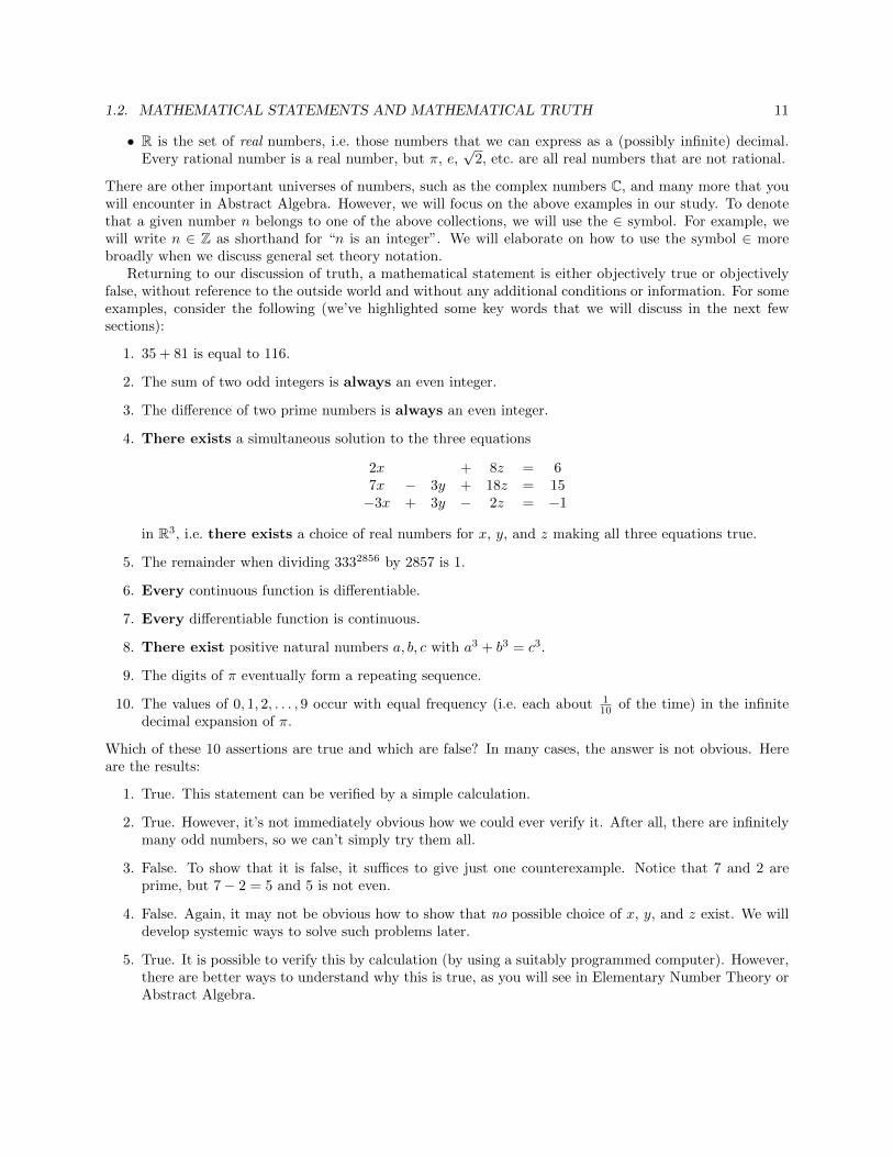
Returning to our discussion of truth, a mathematical statement is either objectively true or objectivelyfalse, without reference to the outside world and without any additional conditions or information. For someexamples, consider the following (we’ve highlighted some key words that we will discuss in the next fewsections):
1. 35 + 81 is equal to 116.
2. The sum of two odd integers is always an even integer.
3. The difference of two prime numbers is always an even integer.
4. There exists a simultaneous solution to the three equations
2x + 8z = 67x − 3y + 18z = 15−3x + 3y − 2z = −1
in R3, i.e. there exists a choice of real numbers for x, y, and z making all three equations true.
5. The remainder when dividing 3332856 by 2857 is 1.
6. Every continuous function is differentiable.
7. Every differentiable function is continuous.
8. There exist positive natural numbers a, b, c with a3 + b3 = c3.
9. The digits of π eventually form a repeating sequence.
10. The values of 0, 1, 2, . . . , 9 occur with equal frequency (i.e. each about 110 of the time) in the infinite
decimal expansion of π.
Which of these 10 assertions are true and which are false? In many cases, the answer is not obvious. Hereare the results:
1. True. This statement can be verified by a simple calculation.
2. True. However, it’s not immediately obvious how we could ever verify it. After all, there are infinitelymany odd numbers, so we can’t simply try them all.
3. False. To show that it is false, it suffices to give just one counterexample. Notice that 7 and 2 areprime, but 7− 2 = 5 and 5 is not even.
4. False. Again, it may not be obvious how to show that no possible choice of x, y, and z exist. We willdevelop systemic ways to solve such problems later.
5. True. It is possible to verify this by calculation (by using a suitably programmed computer). However,there are better ways to understand why this is true, as you will see in Elementary Number Theory orAbstract Algebra.
12 CHAPTER 1. INTRODUCTION
6. False. The function f(x) = |x| is continuous everywhere but is not differentiable at 0.
7. True. See Calculus or Analysis.
8. False. This is a special case of something called Fermat’s Last Theorem, and it is quite difficult toshow (see Algebraic Number Theory).
9. False. This follows from the fact that π is an irrational number, i.e. not an element of Q, but this isnot easy to show.
10. We still don’t know whether this is true or false! Numerical evidence (checking the first billion digitsdirectly, for example) suggests that it may be true. Mathematicians have thought about this problemfor a century, but we still do not know how to answer it definitively.
Recall that a mathematical statement must be either true or false. In contrast, an equation is typicallyneither true nor false when viewed in isolation, and hence is not a mathematical statement. For example,it makes no sense to ask whether y = 2x+ 3 is true or false, because it depends on which numbers we plugin for x and y. When x = 6 and y = 15, then the statement becomes true, but when x = 3 and y = 7, thestatement is false. For a more interesting example, the equation
(x+ y)2 = x2 + 2xy + y2
is not a mathematical statement as given, because we have not been told how to interpret the x and the y.Is the statement true when x is my cat Cayley and y is my cat Maschke? (Adding them together is scaryenough, and I don’t even want to think about what it would mean to square them.) In order to assign atruth value, we need to provide context for where x and y can come from. To fix this, we can write
“For all real numbers x and y, we have (x+ y)2 = x2 + 2xy + y2”,
which is now a true mathematical statement. As we will eventually see, if we replace real numbers with 2×2matrices, the corresponding statement is false.
For a related example, it is natural to think that the statement (x+ y)2 = x2 + y2 is false, but again itis not a valid mathematical statement as written. We can instead say that the statement
“For all real numbers x and y, we have (x+ y)2 = x2 + y2”
is false, because (1 + 1)2 = 4 while 12 + 12 = 2. However, the mathematical statement
“There exist real numbers x and y such that (x+ y)2 = x2 + y2”
is true, because (1 + 0)2 does equal 12 + 02. Surprisingly, there are contexts (i.e. replacing real numbers withmore exotic number systems) where the corresponding “for all” statement is true (see Abstract Algebra).
Here are a few other examples of statements that are not mathematical statements:
• F = ma and E = mc2: Our current theories of physics say that these equations are true in the realworld whenever the symbols are interpreted properly, but mathematics on its own is a different beast.As written, these equations are neither true nor false from a mathematical perspective. For example,if F = 4, m = 1, and a = 1, then F = ma is certainly false.
• a2 + b2 = c2: Unfortunately, most people “remember” this as the Pythagorean Theorem. However, itis not even a mathematical statement as written. We could fix it by writing “For all right triangleswith side lengths a, b, and c, where c is the length the hypotenuse, we have that a2 + b2 = c2”, inwhich case we have a true mathematical statement.
1.2. MATHEMATICAL STATEMENTS AND MATHEMATICAL TRUTH 13
• Talking Heads is the greatest band of all time: Of course, different people can have different opinionsabout this. I may believe that the statement is true, but the notion of “truth” here is very differentfrom the objective notion of truth necessary for a mathematical statement.
• Shakespeare wrote Hamlet: This is almost certainly true, but it’s not a mathematical statement. First,it references the outside world. Also, it’s at least conceivable that with new evidence, we might changeour minds. For example, perhaps we’ll learn that Shakespeare stole the work of somebody else.
In many subjects, a primary goal is to determine whether certain statements are true or false. However,the methods for determining truth vary between disciplines. In the natural sciences, truth is often gaugedby appealing to observations and experiments, and then building a logical structure (perhaps using somemathematics) to convince others of a claim. Economics arguments are built through a combination of currentand historical data, mathematical modeling, and rhetoric. In both of these examples, truth is always subjectto revision based on new evidence.
In contrast, mathematics has a unique way of determining the truth or falsity of a given statement: weprovide an airtight, logical proof that verifies its truth with certainty. Once we’ve succeeded in finding acorrect proof of a mathematical statement, we know that it must be true for all eternity. Unlike the naturalsciences, we do not have tentative theories that are extremely well-supported but may be overthrown withnew evidence. Thus, mathematics does not have the same types of revolutions like plate tectonics, evolutionby natural selection, the oxygen theory of combustion (in place of phlogiston), relativity, quantum mechanics,etc. which overthrow the core structure of a subject and cause a fundamental shift in what statements areunderstood to be true.
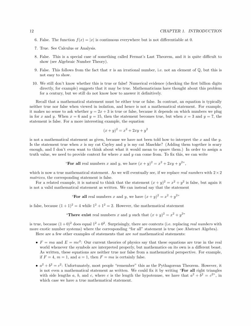
To many, the fact that mathematicians require a complete logical proof with absolute certainty seemsstrange. Doesn’t it suffice to simply check the truth of statement in many instances, and then generalize itto a universal law? Consider the following example. One of the true statements mentioned above is thatthere are no positive natural numbers a, b, c with a3 + b3 = c3, i.e. we can not obtain a cube by addingtwo cubes. The mathematician Leonhard Euler conjectured that a similar statement held for fourth powers,i.e. that we can not obtain a fourth power by adding three fourth powers. More formally, he conjecturedthat there are no positive natural numbers a, b, c, d with a4 + b4 + c4 = d4. For over 200 years it seemedreasonable to believe this might be true, as it held for all small examples and was a natural generalizationof a true statement. However, it was eventually shown that there indeed are examples where the sum of 3fourth powers equals a fourth power, such as the following:
958004 + 2175194 + 4145604 = 4224814.
In fact, this example is the smallest one possible. Thus, even though a4 + b4 + c4 6= d4 for all values positivenatural numbers a, b, c, and d having at most 5 digits, the statement does not hold generally.
In spite of this example, you may question the necessity of proofs for mathematics relevant to the sciencesand applications, where approximations and occasional errors or exceptions may not matter so much. Thereare many historical reasons why mathematicians have embraced complete, careful, and logical proofs as theway to determine truth in mathematics independently from applications. In later math classes, you mayexplore some of these internal historical aspects, but here are three direct reasons for this approach:
• Mathematics should exist independently from the sciences because sometimes the same mathematicsapplies to different subjects. It is possible that edge cases which do not matter in one subject (sayeconomics or physics) might matter in another (like computer science). The math needs to be consistentand coherent on its own without reference to the application.
• In contrast to the sciences where two generally accepted theories that contradict each other in someinstance can coexist for long periods of time (such as relativity and quantum mechanics), mathematicscan not sustain such inconsistencies. As we’ll see, one reason for this is that mathematics allows acertain type of argument called proof by contradiction. Any inconsistency at all would allow us todraw all sorts of erroneous conclusions, and the logical structure of mathematics would unravel.
14 CHAPTER 1. INTRODUCTION
• Unlike the sciences, many areas of math are not subject to direct validation through a physical test. Anidea in physics or chemistry, arising from either a theoretical predication or a hunch, can be verified byrunning an experiment. However, in mathematics we often have no way to reliably verify our guessesthrough such means. As a result, proofs in mathematics can be viewed as the analogues of experimentsin the sciences. In other words, since mathematics exists independently from the sciences, we need aninternal check for our intuitions and hunches, and proofs play this role.
1.3 Quantifiers and Proofs
In the examples of mathematical statements in the previous section, we highlighted two key phrases thatappear incredibly often in mathematical statements: for all and there exists. These two phrases are calledquantifiers in mathematics, and they form the building blocks of more complicated expressions. Occasionally,these quantifiers appear disguised by a different word choice. Here are a few phrases that mean precisely thesame thing in mathematics:
• For all: For every, For any, Every, Always, . . . .
• There exists: There is, For some, We can find, . . . .
These phrases mean what you might expect. For example, saying that a statement of the form “For alla, . . . ” is true means that whenever we plug in any particular value for a into the . . . part, the resultingstatement is true. Similarly, saying that a statement of the form “There exists a, . . . ” is true means thatthere is at least one (but possibly more) choice of a value to plug in for a so that the resulting statement istrue. Notice that we are not saying that there is exactly one choice. Also, be careful in that the phrase “forsome” used in everyday conversation could be construed to mean that there need to be several (i.e. morethan one) values to plug in for a to make the result true, but in math it is completely synonymous with“there exists”.
So how do we prove that a statement that begins with a “there exists” quantifier is true? For example,consider the following statement:
“There exists a ∈ Z such that 2a2 − 1 = 71”.
From your training in mathematics up to this point, you may see the equation at the end and immediatelyrush to manipulate it using the procedures that you’ve been taught for years. Before jumping into that, let’sexamine the logical structure here. As mentioned above, our “there exists” statement is true exactly whenthere is a concrete integer that we can plug in for a so that “2a2 − 1 = 71” is a true statement. Thus, inorder to convince somebody that the statement is true, we need only find (at least) one particular value toplug in for a so that when we compute 2a2−1 we obtain 71. Right? In other words, if all that we care aboutis knowing for sure that the statement is true, we just need to verify that some a ∈ Z has this property.Suppose that we happen to stumble across the number 6 and notice that
2 · 62 − 1 = 2 · 36− 1
= 72− 1
= 71.
At this point, we can assert with confidence that the statement is true, and in fact we’ve just carried outa complete proof. Now you may ask yourself “How did we know to plug in 6 there?”, and that is a goodquestion. However, there is a difference between the creative leap (or leap of faith) we took in choosing 6,and the routine verification that it worked. Perhaps we arrived at 6 by plugging in numbers until we gotlucky. Perhaps we sacrificed a chicken to get the answer. Perhaps we had a vision. Maybe you copied theanswer from a friend or from online (note: don’t do this). Now we do care very much about the underlying
1.3. QUANTIFIERS AND PROOFS 15
methods to find a, both for ethical reasons and because sacrificing a chicken may not work if we change theequation slightly. However, for the logical purposes of this argument, the way that we arrived at our valuefor a does not matter.
We’re (hopefully) all convinced that we have verified that the statement “There exists a ∈ Z such that2a2 − 1 = 71” is true, but as mentioned we would like to have routine methods to solve similar problems inthe future so that we do not have to stumble around in the dark nor invest in chicken farms. Of course, thetools to do this are precisely the material that you learned years ago in elementary algebra. One approachis to perform operations on both sides of the equality with the goal of isolating the a. If we add 1 to bothsides, we arrive at 2a2 = 72, and after dividing both sides by 2 we conclude that a2 = 36. At this point, werealize that there are two solutions, namely 6 and −6. Alternatively, we can try bringing the 71 over andfactoring. By the way, this method found two solutions, and indeed −6 would have worked above. However,remember that proving a “there exists” statement means just finding at least one value that works, so itdidn’t matter that there was more than one solution.
Let’s consider the following more interesting example of a mathematical statement:
“There exists a ∈ R such that 2a5 + 2a3 − 6a2 + 1 = 0”.
It’s certainly possible that we might get lucky and find a real number to plug in that verifies the truth of thisstatement. But if the chicken sacrificing doesn’t work, you may be stymied about how to proceed. However,if you remember Calculus, then there is a nice way to argue that this statement is true without actuallyfinding a particular value of a. The key fact is the Intermediate Value Theorem from Calculus, which saysthat if f : R → R is a continuous function that is positive at some point and negative at another, then itmust be 0 at some point as well. Letting f(x) = 2x5 + 2x3 − 6x2 + 1, we know from Calculus that f(x) iscontinuous. Since f(0) = 1 and f(1) = −1, it follows from the Intermediate Value Theorem that there is ana ∈ R (in fact between 0 and 1) such that f(a) = 0. Thus, we’ve proven that the above statement is true,so long as you accept the Intermediate Value Theorem. Notice again that we’ve established the statementwithout actually exhibiting an a that works.
We can make the above question harder by performing the following small change to the statement:
“There exists a ∈ Q such that 2a5 + 2a3 − 6a2 + 1 = 0”.
Since we do not know what the value of a that worked above was, we are not sure whether it is an elementof Q. In fact, questions like this are a bit harder. There is indeed a method to determine the truth of astatement like this, but that’s for another course (see Abstract Algebra). The takeaway lesson here is thatmathematical statements that look quite similar might require very different methods to solve.
Summing up, a statement of the form “There exists a such that . . . ” is true exactly when there is someconcrete value of a that we can plug into “. . . ” so the resulting statement is true. Thus, saying that thestatement
“There exists a ∈ Z such that 2a2 − 1 = 71”
is true is the same as saying that at least one of the following (infinitely many) mathematical statements istrue:
• . . .
• 2 · (−2)2 − 1 = 71.
• 2 · (−1)2 − 1 = 71.
• 2 · 02 − 1 = 71.
• 2 · 12 − 1 = 71.
16 CHAPTER 1. INTRODUCTION
• 2 · 22 − 1 = 71.
• . . .
Now almost all of these statements are false, but the fact that at least one of them is true (in fact, exactlytwo are true) means that the original “there exists” statement is true.
Let’s move on to statements involving our other quantifier. Consider the following “for all” statement:
“For all a, b ∈ R, we have (a+ b)2 = a2 + 2ab+ b2”.
In the previous section, we briefly mentioned this statement, but wrote it slightly differently as:
“For all real numbers x and y, we have (x+ y)2 = x2 + 2xy + y2”.
Notice that these are both expressing the exact same thing. We only replaced the phrase “real numbers”by the symbol R and changed our choice of letters. Since the letters are just placeholders for the “for all”quantifier, these two mean precisely the same thing. What does it mean to say that the first statement aboveis true? As mentioned above, our “for all” statement is true exactly when whenever we plug in concrete realnumbers for a and b into “2a2 − 1 = 71”, the result is a true statement. In other words, this is the same assaying that every single one of the following (infinitely many) mathematical statements are true:
• . . .
• (3 + 7)2 = 32 + 2 · 3 · 7 + 72.
• (1 + 0)2 = 12 + 2 · 1 · 0 + 02.
• ((−5) + π)2 = (−5)2 + 2 · (−5) · π + π2.
• ((−11) + (−11))2 = (−11)2 + 2 · (−11) · (−11) + (−11)2.
• (e+√
2)2 = e2 + 2 · e ·√
2 + (√
2)2.
• . . .
Notice that we are allowing the possibility of plugging in the same value for both a and b. We use differentletters because they could correspond to different values, not because they must correspond to differentvalues.
Ok, so how do we prove that the statement
“For all a, b ∈ R, we have (a+ b)2 = a2 + 2ab+ b2”.
is true? The problem is that there are infinitely many elements of R (so infinitely many choices for each of aand b), and hence there is no way to examine each possible pair in turn and ever hope to finish. Moreover,there are lots of real numbers that you’ve never thought about before, so it’s hard to even conceive of beingable to work with them all.
The way around this obstacle is write a general argument that works regardless of the values for a and b.In other words, we’re going to take two completely arbitrary elements of R that we will name as a and b (sothat we can refer to them), and then argue that the result of computing (a+ b)2 is the same as the result ofcomputing a2 + 2ab+ b2. When we say “arbitrary”, think about sticking your hand into a bag containing allof the real numbers, and pulling out values for a and b. You are not allowed to pick “nice” values, and youhave to work with anything that comes from the bag. In fact, it might help to think of the values of a and bas being picked out of the bag and handed to you by an evil adversary. By taking these arbitrary elements ofR that we call a and b, and then arguing that the value (a+ b)2 equals the value a2 + 2ab+ b2, our argument
1.3. QUANTIFIERS AND PROOFS 17
will work no matter which particular numbers are actually chosen for a and b. In other words, if we are ableto write a general argument that works using only the assumption that a and b are real numbers (i.e. usingonly the fact that they came from the bag), then we can conclude with confidence that each of the infinitelymany statements written above are true, and hence the “for all” statement is true.
Now in order to do this, we have to start somewhere. After all, with no assumptions at all about how+ and · work, or what squaring means, we have no way to proceed. Ultimately, mathematics starts withbasic axioms explaining how certain fundamental mathematical objects and operations work, and builds upeverything from there. We won’t go into all of those axioms here, but for the purposes of this discussion wewill make use of the following fundamental facts about the real numbers:
• Commutative Law (for multiplication): For all x, y ∈ R, we have x · y = y · x.
• Distributive Law: For all x, y, z ∈ R, we have x · (y + z) = x · y + x · z.
These facts are often taken as two (of about 12) of the axioms for the real numbers. It is also possible toprove them from a construction of the real numbers (see Analysis) using more fundamental axioms. In anyevent, we can use them to prove the above statement as follows. Let a, b ∈ R be arbitrary. We then havethat a+ b ∈ R, and
(a+ b)2 = (a+ b) · (a+ b) (by definition)
= (a+ b) · a+ (a+ b) · b (by the Distributive Law)
= a · (a+ b) + b · (a+ b) (by the Commutative Law)
= a · a+ a · b+ b · a+ b · b (by the Distributive Law)
= a2 + a · b+ a · b+ b2 (by the Commutative Law)
= a2 + 2ab+ b2 (by definition).
Focus on the logic, and not the algebraic manipulations. We begin by taking arbitrary a, b ∈ R. Once thatsentence is complete, a and b each now represent a specific concrete real number. That is, they are no longer“varying” or serving as placeholders for all real numbers. The act of taking arbitrary values fixes them asconcrete numbers, and hence we are now faced with one of mathematical statements in the above infinitelist of mathematical statements.
Now let’s turn our attention to the chain of equalities. Read them in consecutive order. We are claimingthat (a + b)2 equals (a + b) · (a + b) in the first line. Then the second line says that (a + b) · (a + b) equals(a + b) · a + (a + b) · b by the Distributive Law. Here is the underlying logic behind that equality. Noticethat a+ b is some particular real number because a and b are particular real numbers (recall that they wereinstantiated as such when we took arbitrary values at the beginning). Now since a + b is a particular realnumber (think of it as x), and we can view a+ b as the sum of two real numbers (playing the role of y andz, respectively), we can apply the Distributive Law to conclude that (a+ b) · (a+ b) = (a+ b) · a+ (a+ b) · b.The next line is an assertion that the third and fourth expressions are equal by the Commutative Law, etc.If you believe all of the steps, then we have shown that for our completely arbitrary choice of a and b in R,the first and second expressions are equal, the second and third expressions are equal, the third and fourthexpressions are equal, etc. Since equality is transitive (i.e. if x = y and y = z, then x = z), we concludethat (a + b)2 = a2 + 2ab + b2. We have taken completely arbitrary a, b ∈ R, and verified the statement inquestion, so we can now assert that the “For all” statement is true.
As a quick aside, now that we know that (a + b)2 = a2 + 2ab + b2 for all a, b ∈ R, we can use this factwhenever we have two real numbers. We can even conclude that the statement
“For all a, b ∈ R, we have (2a+ 3b)2 = (2a)2 + 2(2a)(3b) + (3b)2”
is true. How does this follow? Consider completely arbitrary a, b ∈ R. We then have that 2a ∈ R and 3b ∈ R,and thus we can apply our previous result to the two numbers 2a and 3b. We are not setting “a = 2a” or
18 CHAPTER 1. INTRODUCTION
“b = 3b” because it does not make sense to say that a = 2a if a is anything other than 0. We are simplyusing the fact that if a and b are real numbers, then 2a and 3b are also real numbers, so we can insertthem in for the placeholder values of a and b in our result. Always think of the (arbitrary) choice of lettersused in “there exists” and “for all” statements as empty vessels that could be filled with any appropriate value.
We’ve discussed the basic idea behind how to prove that a “there exists” statement or a “for all” statementis true. How do we we prove that statements of these forms are false? For example, suppose that we wantto show that the statement
“There exists a ∈ R such that a2 + 2a = −5”
is false. That is, we want to argue that there is no concrete real number that can be plugged into a so thatthe resulting statement “a2 + 2a = −5” is a true statement. In other words, we want to show that none ofthe following (infinitely many) mathematical statements are true:
• . . .
• 32 + 2 · 3 = −5.
• 02 + 2 · 0 = −5.
• (−11)2 + 2 · (−11) = −5.
• e2 + 2 · e = −5.
• (√
2)2 + 2 ·√
2 = −5.
• . . .
Turning this on its head, we want to show that all of the following (infinitely many) mathematical statementsare true:
• . . .
• 32 + 2 · 3 6= −5.
• 02 + 2 · 0 6= −5.
• (−11)2 + 2 · (−11) 6= −5.
• e2 + 2 · e 6= −5.
• (√
2)2 + 2 ·√
2 6= −5.
• . . .
Notice how the word all found its way into the above reasoning. Showing that none of a collection ofstatements is true is the same as showing that all of them are false, which is the same as showing that all ofthe corresponding negations are true! Thinking through the logic, the statement
“There exists a ∈ R such that a2 + 2a = −5”
is false exactly when the statement
“For all a ∈ R, we have a2 + 2a 6= −5”
is true.
1.3. QUANTIFIERS AND PROOFS 19
We made use of negations above by noticing that the negation of the statement “a2 + 2a = −5” is thestatement “a2 + 2a 6= −5”. But we can use the above ideas to understand the negation of more complicatedstatements involving quantifiers. The negation of the statement
“There exists a ∈ R such that a2 + 2a = −5”
is simply“Not(There exists a ∈ R such that a2 + 2a = −5).
However, this statement, with the giant Not in front, is not easily amenable to analysis because it is neithera “there exists” statement nor a “for all” statement. But as we saw above, this negation is equivalent to thestatement
“For all a ∈ R, we have a2 + 2a 6= −5”.
In other words, we can move the negation past the “there exists” as long as we change it to a “for all” whendoing so. Thus, in order to prove that
“There exists a ∈ R such that a2 + 2a = −5”
is false, we can instead prove that
“For all a ∈ R, we have a2 + 2a 6= −5”
is true, because it is equivalent to the negation. And we have a strategy for proving that a “for all” statementis true by working with an arbitrary element! Let’s carry out the argument here. Consider an arbitrarya ∈ R. Notice that
a2 + 2a = (a2 + 2a+ 1)− 1
= (a+ 1)2 − 1
≥ 0− 1 (because squares of reals are nonnegative)
= −1.
We have shown that given any arbitrary a ∈ R, we have a2 +2a ≥ −1, and hence a2 +2a 6= −5. We concludethat the statement
“For all a ∈ R,we have a2 + 2a 6= −5”
is true, and hence the statement
“There exists a ∈ R such that a2 + 2a = −5”
is false. Can you see a way to solve this problem using Calculus?
Everything that we said in this example works generally. That is, suppose that we have a statement ofthe form
“There exists a such that . . . ”,
and we want to argue that the statement is false. We instead prove that the negation
“Not(There exists a such that . . . )”
is true. To show that there does not exist an a with a certain property, we need to show that every a failsto have that property. Thus, we can instead show that the statement
“For all a,we have Not(. . . )”
20 CHAPTER 1. INTRODUCTION
is true.Similarly, suppose that we have a statement of the form
“For all a, we have . . . ”,
and we want to argue that the statement is false. We instead prove that the negation
“Not(For all a, we have . . . )”
is true. To show that not every a has a certain property, we need to show that there exists some a that failsto have that property. Thus, we can instead show that the statement
“There exists a such that Not(. . . )”
is true. In general, we can move a Not past one of our two quantifiers at the expense of flipping the quantifierto the other type. Although this provides a useful mechanical rule to apply when thinking about negations,it is better to think through the underlying logic each time until the reasoning becomes completely natural.
Life becomes more complicated when a mathematical statement involves both types of quantifiers in analternating fashion. For example, consider the following two statements:
1. “For all x ∈ Z, there exists y ∈ Z such that 3x+ y = 5”.
2. “There exists y ∈ Z such that for all x ∈ Z, we have 3x+ y = 5”.
At first glance, these two statements appear to be essentially the same. After all, they both have “for allx ∈ Z”, both have “there exists y ∈ Z”, and both end with the expression “3x+ y = 5”. Does the fact thatthese quantifiers appear in different order matter?
Let’s examine the first statement more closely. Notice that it has the form “For all x ∈ Z . . . ”. In orderfor this “for all”statement to be true, we want to know whether we obtain a true statement whenever weplug in a particular integer x in the “. . . ” part. In other words, we’re asking if all of the following (infinitelymany) mathematical statements are true:
• . . .
• “There exists y ∈ Z such that 3 · (−2) + y = 5”.
• “There exists y ∈ Z such that 3 · (−1) + y = 5”.
• “There exists y ∈ Z such that 3 · 0 + y = 5”.
• “There exists y ∈ Z such that 3 · 1 + y = 5”.
• “There exists y ∈ Z such that 3 · 2 + y = 5”.
• . . .
Looking through each of these, it does indeed appear that they are all true: We can use y = 11 in the firstdisplayed one (i.e. when x = −2), then y = 8 in the next, then y = 5 in the next one, etc. However, thereare infinitely many statements, so we can’t actually check each one in turn and hope to finish. We need ageneral argument that works no matter which value x takes. Now given any arbitrary x ∈ Z, we can verifyif consider the value of y to be 5 − 3x, then we obtain a true statement. Here is how we would write thisargument up formally.
Proposition 1.3.1. For all x ∈ Z, there exists y ∈ Z such that 3x+ y = 5.
1.3. QUANTIFIERS AND PROOFS 21
Proof. Let x ∈ Z be arbitrary. Since Z is closed under multiplication and subtraction, we know that5− 3x ∈ Z. Now
3x+ (5− 3x) = (3x− 3x) + 5
= 0 + 5
= 5.
Thus, we have shown the existence of a y ∈ Z with 3x+ y = 5 (namely y = 5− 3x).
Let’s pause to note a few things about this argument. First, we’ve labeled the statement as a proposition.By doing so, we are making a claim that the statement to follow is a true statement, and that we will beproviding a proof. Alternatively, we sometimes will label a statement as a theorem instead of a propositionif we want to elevate it to a position of prominence (typically theorems say something powerful, surprising,or incredibly useful). In the proof, we are trying to argue that a “for all” statement is true, so we startby taking an arbitrary element of Z. Although this x is arbitrary, it is not varying. Instead, once we takean arbitrary x, it is now one fixed concrete integer that we can use in the rest of the argument. For thisparticular but arbitrary x ∈ Z, we now want to argue that a certain “there exists” statement is true. Inorder to do this, we need to exhibit an example of an y that works, and verify it for the reader. Sincewe have a particular x ∈ N in hand, the y that we pick can depend on that x. In this case, we simplyverify that 5 − 3x works as a value for y. As in the examples given above, we do not need to explain whywe chose to use 5 − 3x, only that the resulting statement is true. That is, although you might have donesome algebra to figure out what y might work, the process you used to find such a potential y is irrele-vant to the logical demonstration that such a y exists. Finally, the square box at the end of the argumentindicates that the proof is over, and so the next paragraph (i.e. this one) is outside the scope of the argument.
Let’s move on to the second of our two statements above. Notice that it has the form “There existsy ∈ Z . . . ”. In order for this statement to be true, we want to know whether we can find one value for y suchthat we obtain a true statement in the “. . . ” part after plugging it in. In other words, we’re asking if any ofthe following (infinitely many) mathematical statements are true:
• . . .
• “For all x ∈ Z, we have 3x+ (−2) = 5”.
• “For all x ∈ Z, we have 3x+ (−1) = 5”.
• “For all x ∈ Z, we have 3x+ 0 = 5”.
• “For all x ∈ Z, we have 3x+ 1 = 5”.
• “For all x ∈ Z, we have 3x+ 2 = 5”.
• . . .
Looking through each of these, it appears that every single one of them is false, i.e. none of them are true.Thus, it appears that the second statement is false. We can formally prove that it is false by proving thatits negation is true. Applying our established rules for how to negate across quantifiers, to show that
“Not(There exists y ∈ Z such that for all x ∈ Z, we have 3x+ y = 5”
is true, we can instead show that
“For all y ∈ Z, Not(for all x ∈ Z, we have 3x+ y = 5)”
22 CHAPTER 1. INTRODUCTION
is true, which is same as showing that
“For all y ∈ Z, there exists x ∈ Z such that Not(3x+ y = 5)”
is true, which is the same as showing that
“For all y ∈ Z, there exists x ∈ Z such that 3x+ y 6= 5”.
is true. We now prove that this final statement is true, which is the same as showing that our original secondstatement is false.
Proposition 1.3.2. For all y ∈ Z, there exists x ∈ Z such that 3x+ y 6= 5.
Proof. Let y ∈ Z be arbitrary. We have two cases:
• Case 1: Suppose that y 6= 5. We then have that 0 ∈ Z and
3 · 0 + y = 0 + y
= y.
Since y 6= 5, we have shown the existence of an x ∈ Z with 3x+ y 6= 5 (namely x = 0).
• Case 2: Suppose that y = 5. We then have that 1 ∈ Z and
3 · 1 + y = 3 + 5
= 8.
Since 8 6= 5, we have shown the existence of an x ∈ Z with 3x+ y 6= 5 (namely x = 1).
As these two cases exhaust all possibilities for y, we have shown that such an x exists unconditionally.
Again, let’s pause to examine the structure of this proof. Since we are trying to prove a “for all”statement, we start by taking an arbitrary element of Z. Once we have this y in hand, our task is to prove a“there exists” statement. Intuitively, once we have a specific y in hand, i.e. once y is given a concrete value,it appears that almost any value of x will work. In fact, it seems that at most one value of x might cause aproblem. But our task is to prove a “there exists” statement, so we need to provide a value of x and provethat it works. In the above argument, we chose to respond to the given y with the value of x = 0, so long asthe given value of y is not 5. Why did make this case distinction and use this particular value of x? Fromthe logical perspective of the argument, our motivations do not matter. Of course, it is a good exercise toconsider why the case distinction was made, and what motivated the choice of x. That’s not to say thatthese are the only choices we could make! It is certainly possible to make a different case distinction and/orchoose different values of x in response to specific y’s. Try to write a different argument yourself!
In general, consider statements of the following two types:
1. “For all a, there exists b such that . . . ”.
2. “There exists b such that for all a, we have . . . ”.
Let’s examine the difference between them in a more informal way. Think about a game with two playerswhere Player I goes first. For the first statement to be true, it needs to be the case that no matter howPlayer I moves, Player II can respond in such a way so that . . . happens. Notice in this scenario PlayerII’s move can depend on Player I’s move, i.e. the value of b can depend on the value of a. For the secondstatement to be true, it needs to be the case that Player I can make a move so brilliant that no matter howPlayer II responds, we have that . . . happens. In this scenario, b needs to be chosen first without knowing
1.3. QUANTIFIERS AND PROOFS 23
a, so b can not depend on a in any way.
Finally, let’s discuss one last construct in mathematical statements, which is an “if...then...” clause. Wecall such statements implications, and they naturally arise when we want to quantify only over part of a set.For example, the statement
“For all a ∈ R, we have a2 − 4 ≥ 0”
is false because 0 ∈ R and 02 − 4 < 0. However, the statement
“For all a ∈ R with a ≥ 2, we have a2 − 4 ≥ 0”
is true. Instead of coupling the condition “a ≥ 2” with the “for all” statement, we can instead write thisstatement as
“For all a ∈ R, (If a ≥ 2, then a2 − 4 ≥ 0)”.
We often write this statement in shorthand by dropping the “for all” as:
“If a ∈ R and a ≥ 2, then a2 − 4 ≥ 0”.
One convention, that initially seems quite strange, arises from this. Since we want to allow “if...then...”statements, we need to assign truth values to them because every mathematical statement should eitherbe true or false. If we plug the value 3 for a into this last statement (or really past the “for all” in thepenultimate statement), we arrive at the statement
“If 3 ≥ 2, then 32 − 4 ≥ 0”,
which we naturally say is true because both the “if” part and the “then” part are true. However, it’s lessclear how we should assign a truth value to
“If 1 ≥ 2, then 12 − 4 ≥ 0”
because both the “if” part and the “then” part are false. We also have an example like
“If − 5 ≥ 2, then (−5)2 − 4 ≥ 0”,
where the “if” part is false and the “then” part is true. In mathematics, we make the convention that an“if...then...” statement is false only when the “if” part is true and the “then” part is false. Thus, these lasttwo examples we declare to be true. The reason why we do this is be consistent with the intent of the “forall” quantifier. In the example
“For all a ∈ R, (If a ≥ 2, then a2 − 4 ≥ 0)”,
we do not want values of a with a < 2 to have any effect at all on the truth value of the “for all” statement.Thus, we want the parenthetical statement to be true whenever the “if” part is false. In general, given twomathematical statements P and Q, we define the following:
• If P is true and Q is true, we say that “If P , then Q” is true.
• If P is true and Q is false, we say that “If P , then Q” is false.
• If P is false and Q is true, we say that “If P , then Q” is true.
• If P is false and Q is false, we say that “If P , then Q” is true.
We can compactly illustrate these conventions with the following simple table, known as a truth table,where we use T for true and F for false:
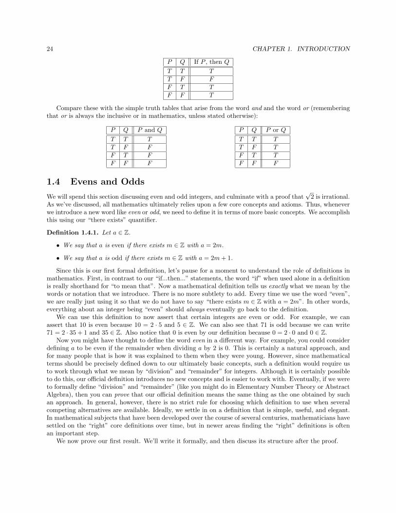
24 CHAPTER 1. INTRODUCTION
P Q If P , then Q
T T TT F FF T TF F T
Compare these with the simple truth tables that arise from the word and and the word or (rememberingthat or is always the inclusive or in mathematics, unless stated otherwise):
P Q P and Q
T T TT F FF T FF F F
P Q P or Q
T T TT F TF T TF F F
1.4 Evens and Odds
We will spend this section discussing even and odd integers, and culminate with a proof that√
2 is irrational.As we’ve discussed, all mathematics ultimately relies upon a few core concepts and axioms. Thus, wheneverwe introduce a new word like even or odd, we need to define it in terms of more basic concepts. We accomplishthis using our “there exists” quantifier.
Definition 1.4.1. Let a ∈ Z.
• We say that a is even if there exists m ∈ Z with a = 2m.
• We say that a is odd if there exists m ∈ Z with a = 2m+ 1.
Since this is our first formal definition, let’s pause for a moment to understand the role of definitions inmathematics. First, in contrast to our “if...then...” statements, the word “if” when used alone in a definitionis really shorthand for “to mean that”. Now a mathematical definition tells us exactly what we mean by thewords or notation that we introduce. There is no more subtlety to add. Every time we use the word “even”,we are really just using it so that we do not have to say “there exists m ∈ Z with a = 2m”. In other words,everything about an integer being “even” should always eventually go back to the definition.
We can use this definition to now assert that certain integers are even or odd. For example, we canassert that 10 is even because 10 = 2 · 5 and 5 ∈ Z. We can also see that 71 is odd because we can write71 = 2 · 35 + 1 and 35 ∈ Z. Also notice that 0 is even by our definition because 0 = 2 · 0 and 0 ∈ Z.
Now you might have thought to define the word even in a different way. For example, you could considerdefining a to be even if the remainder when dividing a by 2 is 0. This is certainly a natural approach, andfor many people that is how it was explained to them when they were young. However, since mathematicalterms should be precisely defined down to our ultimately basic concepts, such a definition would require usto work through what we mean by “division” and “remainder” for integers. Although it is certainly possibleto do this, our official definition introduces no new concepts and is easier to work with. Eventually, if we wereto formally define “division” and “remainder” (like you might do in Elementary Number Theory or AbstractAlgebra), then you can prove that our official definition means the same thing as the one obtained by suchan approach. In general, however, there is no strict rule for choosing which definition to use when severalcompeting alternatives are available. Ideally, we settle in on a definition that is simple, useful, and elegant.In mathematical subjects that have been developed over the course of several centuries, mathematicians havesettled on the “right” core definitions over time, but in newer areas finding the “right” definitions is oftenan important step.
We now prove our first result. We’ll write it formally, and then discuss its structure after the proof.
1.4. EVENS AND ODDS 25
Proposition 1.4.2. If a ∈ Z is even, then a2 is even.
Proof. Let a ∈ Z be an arbitrary even integer. Since a is even,we can fix n ∈ Z with a = 2n. Notice that
a2 = (2n)2
= 4n2
= 2 · (2n2).
Since 2n2 ∈ Z, we conclude that a2 is even.
When starting this proof, we have to remember that there is a hidden “for all” in the “if...then...”. Thatis, the statement that we are trying to prove is:
“For all a ∈ Z, if a is even, then a2 is even”.
Thus, we should start the argument by taking an arbitrary a ∈ Z. However, we’re trying to prove an“if...then...” statement about such an a. Whenever the “if...” part is false, we do not care about it (oralternatively we assign it true by the discussion at the end of the previous section), so instead of taking anarbitrary a ∈ Z, we should take an arbitrary a ∈ Z that is even. With this even a in hand, our goal is toprove that a2 is even.
Recall that whenever we think about even numbers now, we should always eventually go back to ourdefinition. Thus, we next unwrap what it means to say that “a is even”. By definition of even, we know thatthere exists m ∈ Z with a = 2m. In other words, there is at least one choice of m ∈ Z so that the statement“a = 2m” is true.
Now it’s conceivable that there are many m that work (the definition does not rule that out), but thereis at least one that works. We invoke this true statement by picking some value of m ∈ Z that works, and wedo this by giving it a name n. This was an arbitrary choice of name, and we could have chosen almost anyother name for it. We could have called it k, b, `, x, δ, Maschke, ♥, or $. The only really awful choice wouldbe to call it a, because we have already given the letter a a meaning (namely as our arbitrary element). Wecould even have called it m, and in the future we will likely do this. However, to avoid confusion in our firstarguments, we’ve chosen to use a different letter than the one in the definition to make it clear that we arenow fixing one value that works. We encapsulate this entire paragraph in the key phrase “we can fix”. Ingeneral, when we want to invoke a true “there exists” statement in our argument, we use the phrase we canfix to pick a corresponding witness.
Ok, we’ve successfully taken our assumption and unwrapped it, so that we now have a fixed n ∈ Z witha = 2n. Before jumping into the algebra of the middle part of the argument, let’s think about our goal. Wewant to show that a2 is even. In other words, we want to argue that there exists m ∈ Z with a2 = 2m.Don’t think about the letter. We want to end by writing a2 = 2 where we whatever we fill in for is aninteger.
With this in mind, we start with what we know is true, i.e. that a = 2n, and hope to drive forwardwith true statements every step of the way until we arrive at our goal. Since a = 2n is true, we know thata2 = (2n)2 is true. We also know that (2n)2 = 4n2 is true and that 4n2 = 2 · (2n2) is true. Putting it alltogether, we conclude that a2 = 2 · (2n2) is true. Have we arrived at our goal? We’ve written a2 as 2 timessomething, namely it is 2 times 2n2. Finally, we notice that 2n2 ∈ Z because n ∈ Z. Thus, starting with thetrue statement a = 2n, we have derived a sequence of true statements culminating with the true statementthat a2 equals 2 times some integer. Therefore, by definition, we are able to conclude that a2 is even. Sincea was arbitrary, we are done.
Pause to make sure that you understand all of the logic in the above argument. Mathematical proofsare typically written in very concise ways where each word matters. Furthermore, these words often pack incomplex thoughts, such as with the “we can fix” phrase above. Eventually, we will just write our arguments
26 CHAPTER 1. INTRODUCTION
succinctly without all of this commentary, and it’s important to make sure that you understand how tounpack both the language and the logic used in proofs.
In fact, we can prove a stronger result than what is stated in the proposition. It turns out that if a ∈ Zis even and b ∈ Z is arbitrary, then ab is even (i.e. the product of an even integer and any integer is an eveninteger). Try to give a proof! From this fact, we can immediately conclude that the previous proposition istrue, because given any a ∈ Z that is even, we can apply this stronger result when using a for both of thevalues (i.e. for both a and b). Remember that the letters are placeholders, so we can fill them both with thesame value if we want. Different letters do not necessarily mean different values!
Let’s move on to another argument that uses the definitions of both even and odd.
Proposition 1.4.3. If a ∈ Z is even and b ∈ Z is odd, then a+ b is odd.
Proof. Let a, b ∈ Z be arbitrary with a even and b odd. Since a is even, we can fix n ∈ Z with a = 2n. Sinceb is odd, we can fix k ∈ Z with b = 2k + 1. Notice that
a+ b = 2n+ (2k + 1)
= (2n+ 2k) + 1
= 2 · (n+ k) + 1.
Now n+ k ∈ Z because both n ∈ Z and k ∈ Z, so we can conclude that a+ b is odd.
This argument is similar to the last one, but now we have two arbitrary elements a, b ∈ Z, with theadditional assumption that a is even and b is odd. As in the previous proof, we unwrapped the definitionsinvolving “there exists” quantifiers to fix witnessing elements n and k. Notice that we had to give thesewitnessing elements different names because the n that we pick to satisfy a = 2n might be a completelydifferent number from the k that we pick to satisfy b = 2k+ 1. Once we’ve unwrapped those definitions, ourgoal is to prove that a + b is odd, which means that we want to show that a + b = 2 + 1, where we fillin with an integer. Now using algebra we proceed forward from our given information to conclude thata+ b = 2 · (n+ k) + 1, so since n+ k ∈ Z (because both n ∈ Z and k ∈ Z), we have reached our goal.
We now ask a seemingly simple question: Is 1 even? We might notice that 1 is odd because 1 = 2·0+1 and0 ∈ Z, but how does that help us? At the moment, we only have our definitions, and it is not immediatelyobvious from the definitions that a number can not be both even and odd. To prove that 1 is not even, wehave to argue that
“There exists m ∈ Z with 1 = 2m”
is false, which is the same as showing that
“Not(There exists m ∈ Z with 1 = 2m)”
is true, which is the same as showing that
“For all m ∈ Z, we have 1 6= 2m”
is true. Thus, we need to prove a “for all” statement, which we do by considering two cases.
Proposition 1.4.4. The integer 1 is not even.
Proof. We show that 2m 6= 1 for all m ∈ Z. Let m ∈ Z be arbitrary. We then have that either m ≤ 0 orm ≥ 1, giving us two cases:
• Case 1: Suppose that m ≤ 0. Multiplying both sides by 2, we see that 2m ≤ 0, so 2m 6= 1.
• Case 2: Suppose that m ≥ 1. Multiplying both sides by 2, we see that 2m ≥ 2, so 2m 6= 1.
1.4. EVENS AND ODDS 27
Since these two cases exhaust all possibilities for m, we have shown that 2m 6= 1 unconditionally.
This is a perfectly valid argument, but it’s very specific to the number 1. We would like to prove thefar more general result that no integer is both even and odd. We’ll introduce a new method of proof toaccomplish this task. Up until this point, if we have a statement P that we want to prove is true, we tacklethe problem directly by working through the quantifiers one by one. Similarly, if we want to prove that Pis false, we instead prove that Not(P) is true, and use our rules for moving the Not inside so that we canprove a statement involving quantifiers on the outside directly.
However, there is another method to prove that a statement P is true that is beautifully sneaky. Theidea is as follows. We assume that Not(P) is true, and show that under this assumption we can logicallyderive another statement, say Q, that we know to be false. Thus, if Not(P) was true, then Q would have tobe both true and false at the same time. Madness would ensue. Human sacrifice, dogs and cats livingtogether, mass hysteria. This is inconceivable, so the only possible explanation is that Not(P) must befalse, which is the same as saying that P must be true. A proof of this type is called a proof by contradiction,because under the assumption that Not(P) was true, we derived a contradiction, and hence we can concludethat P must be true.
Proposition 1.4.5. No integer is both even and odd.
Before jumping into the proof, let’s examine what the proposition is saying formally. If we write it outcarefully, the claim is that
“Not(There exists a ∈ Z such that a is even and a is odd)”
is true. If we were trying to prove this statement directly, we would move the Not inside and instead try toprove that
“For all a ∈ Z, we have Not(a is even and a is odd)”
is true, which is the same as showing that
“For all a ∈ Z, either a is not even or a is not odd”
is true (recalling that “or” is always the inclusive or in mathematics). To prove this directly, we would thenneed to take an arbitrary a ∈ Z, and argue that (at least one) of “a is not even” or “a is not odd” is true.Since this looks a bit difficult, let’s think about how we would structure a proof by contradiction. Recallthat we are trying to prove that
“Not(There exists a ∈ Z such that a is even and a is odd)”
is true. Now instead of moving the Not inside and proving the corresponding “for all” statement directly,we are going to do a proof by contradiction. Thus, we assume that
“Not(Not(There exists a ∈ Z such that a is even and a is odd))”,
is true, which is the same as assuming that
“There exists a ∈ Z such that a is even and a is odd”,
is true, and then derive a contradiction. Let’s do it.
Proof of Proposition 1.4.5. Assume, for the sake of obtaining a contradiction, that there exists an integerthat is both even and odd. We can then fix an a ∈ Z that is both even and odd. Since a is even, we canfix m ∈ Z with a = 2m. Since a is odd, we can fix n ∈ Z with a = 2n + 1. We then have 2m = 2n + 1, so2(m−n) = 1. Notice that m−n ∈ Z because both m ∈ Z and n ∈ Z. Thus, we can conclude that 1 is even,which contradicts Proposition 1.4.4. Therefore, our assumption must be false, and hence no integer can beboth even and odd.
28 CHAPTER 1. INTRODUCTION
Ok, so no integer can be both even and odd. Is it true that every integer is either even or odd? Intuitively,the answer is clearly yes, but it’s not obvious how to prove it without developing a theory of division withremainder. It is possible to accomplish this task by carrying out the steps in the following outline:
1. Start with 0. We know from above that 0 is even, so clearly 0 is either even or odd.
2. Show that if a ∈ N is either even or odd, then a+ 1 is either even or odd.
3. Intuitively, every natural number can be obtain by starting with 0, and then iteratively adding 1some finite number of times. Thus, using (1) and (2) repeatedly, it seems that we can concludethat every a ∈ N is either even or odd. The way to formalize this argument is to use a techniquecalled “mathematical induction”. However, since a careful discussion of this technique will take ustoo far afield, we will leave the details of the argument to a later courses (see Bridges to AdvancedMathematics).
4. Show that if a ∈ N is either even or odd, then −a is either even or odd. This then allows us to extendthe statement in (3) from N to Z.
Since we are leaving the details of part (3) to a later course, we will simply assert that the following is true,and you’ll have to suffer through the anticipation for a semester.
Fact 1.4.6. Every integer is either even or odd.
We turn now to another result, which will require a new technique to prove.
Proposition 1.4.7. If a ∈ Z and a2 is even, then a is even.
Before jumping into a proof of this fact, we pause to notice that a direct approach looks infeasible. Why?Suppose that we try to prove it directly by starting with the assumption that a2 is even. Then, by definition,we can fix n ∈ Z with a2 = 2n. Since a2 ≥ 0, we conclude that we must have that n ≥ 0. It is now naturalto take the square root of both sides and write a =
√2n. Recall that our goal is to write a as 2 times some
integer, but this looks bad. we have a =√
2 ·√n, but
√2 is not 2, and
√n is probably not an integer. We
can force a 2 by noticing that√
2n = 2 ·√
n2 , but
√n2 seems even less likely to be an integer.
Let’s take a step back. Notice that Proposition 1.4.7 looks an awful lot like Proposition 1.4.2. In fact,one is of the form “If P, then Q” while the other is of the form “If Q, then P”. We say that “If Q, then P”is the converse of “If P, then Q”. Unfortunately, if an “If...then...” statement is true, its converse might befalse. For example,
“If f(x) is differentiable, then f(x) is continuous”
is true, but“If f(x) is continuous, then f(x) is differentiable”.
is false. For an even more basic example, the statement
“If a ∈ Z and a ≥ 7, then a ≥ 4”
is true, but the converse statement
“If a ∈ Z and a ≥ 4, then a ≥ 7”
is false.The reason why Proposition 1.4.2 was easier to prove was that we started with the assumption that a
was even, and by squaring both sides of a = 2n we were able to write a2 as 2 times an integer by using thefact that the square of a integer was an integer. However, starting with an assumption about a2, it seemsdifficult to conclude much about a without taking square roots. Here’s where a truly clever idea comes in.
1.4. EVENS AND ODDS 29
Instead of looking at the converse of our statement, which says “If a ∈ Z and a is even, then a2 is even”,consider the following statement:
“If a ∈ Z and a is not even, then a2 is not even”
Now this statement is a strange twist on the first. We’ve switched the hypothesis and conclusion around andincluded negations that were not there before. At first sight, it may appear that this statement has nothingto do with the one in Proposition 1.4.7. However, suppose that we are somehow able to prove it. I claimthat Proposition 1.4.7 follows. How? Suppose that a ∈ Z is such that a2 is even. We want to argue that amust be even. Well, suppose not. Then a is not even, so by this new statement (which we are assuming weknow is true), we could conclude that a2 is not even. However, this contradicts our assumption. Therefore,it must be the case that a is even!
We want to give this general technique a name. The contrapositive of a statement of the form “If P, thenQ” is the statement “If Not(Q), then Not(P)”. In other words, we flip the two parts of the “If...then...”statement and put a Not on both of them. In general, suppose that we are successful in proving that thecontrapositive statement
“If Not(Q), then Not(P)”
is true. From this, it turns out that we can conclude that
“If P, then Q”
is true. Let’s walk through the steps. Remember, we are assuming that we know that “If Not(Q), thenNot(P)” is true. To prove that “If P, then Q” is true, we assume that P is true, and have as our goal toshow that Q is true. Now under the assumption that Q is false, we would be able to conclude that Not(Q)is true, but this would imply that Not(P) is true, contradicting the fact that we are assuming that P is true!The only logical possibility is that the truth of P must imply the truth of Q.
We are now ready to prove Proposition 1.4.7.
Proof of 1.4.7. We prove the contrapositive. That is, we show that whenever a is not even, then a2 is noteven. Let a ∈ Z be an arbitrary integer that is not even. Using Fact 1.4.6, it follows that a is odd. Thus, wecan fix n ∈ Z with a = 2n+ 1. We then have
a2 = (2n+ 1)2
= 4n2 + 4n+ 1
= 2 · (2n2 + 2n) + 1.
Notice that 2n2 + 2n ∈ Z because n ∈ Z, so we can conclude that a2 is odd. Using Proposition 1.4.5, itfollows that a2 is not even. We have shown that if a is not even, then a2 is not even. Since we’ve proven thecontrapositive, it follows that if a2 is even, then a is even.
We can now prove the following fundamental theorem.
Theorem 1.4.8. There does not exist q ∈ Q with q2 = 2. In other words,√
2 is irrational.
Proof. Suppose for the sake of obtaining a contradiction that there does exist q ∈ Q with q2 = 2. Fix a, b ∈ Zwith q = a
b and such that ab is in lowest terms, i.e. where a and b have no common factors greater than 1.
We have (ab
)2= 2,
hencea2
b2= 2,
30 CHAPTER 1. INTRODUCTION
and so
a2 = 2 · b2.
Since b2 ∈ Z, we conclude that a2 is even. Using Proposition 1.4.7, it follows that a is even, so we can fixc ∈ Z with a = 2c. We then have
2b2 = a2
= (2c)2
= 4c2.
Dividing each side by 2, we conclude that
b2 = 2c2.
Since c2 ∈ Z, it follows that b2 is even. Using Proposition 1.4.7 again, we conclude that b is even. Thus, wecan fix d ∈ Z with b = 2d. We then have
q =a
b=
2c
2d=c
d.
This is a contradiction because ab was assumed to be in lowest terms, but we have reduced it further.
Therefore, there does not exist q ∈ Q with q2 = 2.
We end this section with an interesting fact, which gives another example of proving a “there exists”statement.
Proposition 1.4.9. If a ∈ Z is odd, then there exist b, c ∈ Z with a = b2 − c2. In other words, every oddinteger is the difference of two perfect squares.
Before jumping into the proof, we first try out some examples:
1 = 12 − 02
3 = 22 − 12
5 = 32 − 22
7 = 42 − 32
9 = 52 − 42.
There seems to be a clear pattern here, but notice that 9 = 32 − 02 as well, so there are sometimes otherways to write numbers as the difference of squares. Nonetheless, to prove a “there exists” statement, we justneed to give an example. The above pattern suggests that we can just use adjacent numbers for b and c,and we now give a proof of this fact generally.
Proof. Let a ∈ Z be an arbitrary odd integer. By definition, we can fix n ∈ Z with a = 2n+ 1. Notice thatn+ 1 ∈ Z and that
(n+ 1)2 − n2 = n2 + 2n+ 1− n2
= 2n+ 1
= a.
Therefore, we shown the existence of b and c (namely b = n+1 and c = n) for which a = b2−c2. Since a ∈ Zwas an arbitrary odd integer, we conclude that every odd integer is the difference of two perfect squares.
1.5. SETS, SET CONSTRUCTION, AND SUBSETS 31
1.5 Sets, Set Construction, and Subsets
Sets and Set Construction
We now discuss that fundamental structure that mathematicians use to package objects together.
Definition 1.5.1. A set is a collection of elements without regard to repetition or order.
Intuitively, a set is a box where the only thing that matters are the objects that are inside it, andfurthermore the box does not have more than one of any given object. We use { and } as delimiters for sets.For example, {3, 5} is a set with two elements. Since all that matters are the elements, we define two setsto be equal if they have the same elements, regardless of how the sets themselves are defined or described.
Definition 1.5.2. Given two sets A and B, we say that A = B if A and B have exactly the same elements.
Since the elements themselves matter, but not their order, we have {3, 7} = {7, 3} and {1, 2, 3} = {3, 1, 2}.Also, although we typically would not even write something like {2, 5, 5}, if we choose to do so then we wouldhave {2, 5, 5} = {2, 5} because both have the same elements, namely 2 and 5.
Notation 1.5.3. Given an object x and a set A, we write x ∈ A to mean that x is an element of A, and wewrite x /∈ A to mean that x is not an element of A.
For example, we have 2 ∈ {2, 5} and 3 /∈ {2, 5}. Since sets are mathematical objects, they may beelements of other sets. For example, we can form the set S = {1, {2, 3}}. Notice that we have 1 ∈ S and{2, 3} ∈ S, but 2 /∈ S and 3 /∈ S. As a result, S has only 2 elements, namely 1 and {2, 3}. Thinking of a setas a box, one element of S is the number 1, and the other is a different box (which happens to have the twoelements 2 and 3 inside it).
The empty set is the unique set with no elements. We can write it as {}, but instead we typically denoteit by ∅. There is only one empty set, because if both A and B have no elements, then they have exactly thesame elements for vacuous reasons, and hence A = B. Notice that {∅} does not equal ∅. After all, {∅} hasone element! You can think of {∅} as a box that has one empty box inside it.
Notice that sets can be either finite or infinite. At this point, our standard examples of infinite sets arethe various universes of numbers:
• N = {0, 1, 2, 3, . . . }.
• N+ = {1, 2, 3, . . . }.
• Z = {. . . ,−3,−2,−1, 0, 1, 2, 3, . . . }.
• Q is the set of rational numbers.
• R is the set of real numbers.
Beyond these fundamental sets, there are various ways to define new sets. In some cases, we can simplylist the elements as we did above. Although this often works for small finite sets, it is almost never a goodidea to list the elements of a set with 20 or more elements, and it rarely works for infinite sets (unless thereis an obvious pattern like {5, 10, 15, 20, . . . }). One of the standard ways to define a set S is to carve it outof some bigger set A by describing a certain property that may or may not be satisfied by an element of A.For example, we could define
S = {n ∈ N : 5 < n < 13}.
We read this line by saying that S is defined to be the set of all n ∈ N such that 5 < n < 13. Thus, in thiscase, we are taking A = N, and forming a set S by carving out those elements of A that satisfy the conditionthat 5 < n < 13. In other words, think about going through each of element n, checking if 5 < n < 13 is a
32 CHAPTER 1. INTRODUCTION
true statement, and collecting those n ∈ N that make it true into a set that we call S. In more simple terms,we can also describe S as follows:
S = {6, 7, 8, 9, 10, 11, 12}.
It is important that we put the “N” in the above description, because if we wrote {n : 5 < n < 13} thenit would be unclear what n we should consider. For example, should 11
2 be in this set? How about√
17?Sometimes the “universe” of numbers (or other mathematical objects) that we are working within is clear,but typically it is best to write the global set that we are picking elements from in order to avoid suchambiguity. Notice that when we define a set, there is no guarantee that it has any elements. For example,{q ∈ N : q2 = 2} = ∅ by Theorem 1.4.8. Keep in mind that we can also use words in our description of sets,such as {n ∈ N : n is an even prime}. As mentioned above, two sets that have quite different descriptionscan be equal. For example, we have
{n ∈ N : n is an even prime} = {n ∈ N : 3 < n2 < 8}
because both sets equal {2}. Always remember the structure of sets formed in this way. We write
{x ∈ A : P(x)}
where A is a known set and P(x) is a “property” such that given a particular y ∈ A, the statement P(y) iseither true or false.
Another way to describe a set is through a “parametric” description. Rather than carving out a certainsubset of a given set by describing a property that the elements must satisfy, we can instead form all theelements one obtains by varying a value through a particular set. For example, consider the followingdescription of a set:
S = {3x2 + 1 : x ∈ R}.
Although the notation looks quite similar to the above (in both case we have curly braces, with a : in themiddle), this set is described differently. Notice that instead of having a set that elements are coming fromon the left of the colon, we now have a set that elements are coming from on the right. Furthermore, wenow have a formula on the left rather than a property on the right. The difference is that for a property,when we plug in an element from the given set, we either obtain a true or false value, but that isn’t the casefor a formula like 3x2 + 1. The idea here is that instead of carving out a subset of R by using a property(i.e. taking those elements that make the property true), we let x vary through all real numbers, plug eachof these real numbers x into 3x2 + 1, and form the set of all possible outputs. For example, we have 4 ∈ Sbecause 4 = 3 · 12 + 1. In other words, when x = 1, the left hand side gives the value 4, so we should put4 ∈ S. Notice also that 4 = 3 · (−1)2 + 1, so we can also see that 4 ∈ S because of the “witness” −1. Ofcourse, we are forming a set, so we do not repeat the number 4. We also have 1 ∈ S because 1 = 3 · 02 + 1,and we have 76 ∈ S because 76 = 3 · 52 + 1. Notice also that 7 ∈ S because 7 = 3 · (
√2)2 + 1.
In a general parametric set description, we will have a set A and a function f(x) that allows inputs fromA, and we write
{f(x) : x ∈ A}
for the set of all possible outputs of the function as we vary the inputs through the set A. We will discussthe general definition of a function in the next section, but for the moment you can think of them as givenby formulas.
Now it is possible and indeed straightforward to turn any parametric description of a set into one wherewe carve out a subset by a property. In our case of S = {3x2 + 1 : x ∈ R} above, we can alternatively writeit as
S = {y ∈ R : There exists x ∈ R with y = 3x2 + 1}.
1.5. SETS, SET CONSTRUCTION, AND SUBSETS 33
Notice how we flipped the way we described the set by introducing a “there exists” quantifier in order toform a property. This is always possible for a parametric description. For example, we have
{5n+ 4 : n ∈ N} = {m ∈ N : There exists n ∈ N with m = 5n+ 4}.
Thus, these parametric descriptions are not essentially new ways to describe sets, but they can often be moreconcise and clear.
By the way, we can use multiple parameters in our description. For example, consider the set
S = {18m+ 33n : m,n ∈ Z}.
Now we are simply letting m and n vary through all possible values in Z and collecting all of the values18m+ 33n that result. For example, we have 15 ∈ S because 15 = 18 · (−1) + 33 · 1. We also have 102 ∈ Sbecause 102 = 18 · 2 + 33 · 2. Notice that we are varying m and n independently, so they might take differentvalues, or the same value (as in the case of m = n = 2). Don’t be fooled by the fact that we used differentletters! As above, we can flip this description around by writing
S = {k ∈ Z : There exists m,n ∈ Z with k = 18m+ 33n}.
Subsets and Set Equality
Definition 1.5.4. Given two sets A and B, we write A ⊆ B to mean that every element of A is an elementof B. More formally, A ⊆ B means that for all a ∈ A, we have a ∈ B.
To prove that A ⊆ B, one takes an arbitrary a ∈ A, and argues that a ∈ B. For example, let A = {6n :n ∈ Z} and let B = {2n : n ∈ Z}. Since both of these sets are infinite, we can’t show that A ⊆ B by takingeach element of A in turn and showing that it is an element of B. Instead, we take an arbitrary a ∈ A, andshow that a ∈ B. Here’s the proof.
Proposition 1.5.5. Let A = {6n : n ∈ Z} and B = {2n : n ∈ Z}. We have A ⊆ B.
Proof. Let a ∈ A be arbitrary. By definition of A, this means that we can fix an m ∈ Z with a = 6m. Noticethen that a = 2 · (3m). Since 3m ∈ Z, it follows that a ∈ B. Since a ∈ A we arbitrary, we conclude thatA ⊆ B.
As usual, pause to make sure that you understand the logic of the argument above. First, we took anarbitrary element a from the set A. Now since A = {6n : n ∈ Z} and this is a parametric description withan implicit “there exists” quantifier, there must be one fixed integer value of n that puts a into the set A.In our proof, we chose to call that one fixed integer m. Now in order to show that a ∈ B, we need to exhibita k ∈ Z with a = 2k. In order to do this, we hope to manipulate a = 6m to introduce a 2, and ensure thatthe element we are multiplying by 2 is an integer.
What would go wrong if we tried to prove that B ⊆ A? Let’s try it. Let b ∈ B be arbitrary. Since b ∈ B,we can fix m ∈ Z with b = 2m. Now our goal is to try to prove that we can find an n ∈ Z with b = 6n. It’snot obvious how to obtain a 6 from that 2, but we can try to force a 6 in the following way. Since b = 2mand 2 = 6
3 , we can write b = 6 · m3 . We have indeed found a number n such that b = 6n, but we have notchecked that this n is an integer. In general, dividing an integer by 3 does not result in an integer, so thisargument currently has a hole in it.
Although that argument has a problem, we can not immediately conclude that B 6⊆ A. Our failure tofind an argument does not mean that an argument does not exist. So how can we show that B 6⊆ A? All thatwe need to do is find just one example of an element of B that is not an element of A (because the negationof the “for all” statement A ⊆ B is a “there exists” statement). We choose 2 as our example. However,
34 CHAPTER 1. INTRODUCTION
we need to convince everybody that this choice works. So let’s do it! First, notice that 2 = 2 · 1, so 2 ∈ Bbecause 1 ∈ Z. We now need to show that 2 /∈ A, and we’ll do this using a proof by contradiction. Supposeinstead that 2 ∈ A. Then, by definition, we can fix an m ∈ Z with 2 = 6m. We then have that m = 2
6 = 13 .
However, this a contradiction because 13 /∈ Z. Since our assumption that 2 ∈ A led to a contradiction, we
conclude that 2 /∈ A. We found an example of an element that is in B but not in A, so we conclude thatB 6⊆ A.
Recall that two sets A and B are defined to be equal if they have the same elements. Therefore, we haveA = B exactly when both A ⊆ B and B ⊆ A are true. Thus, given two sets A and B, we can prove thatA = B by performing two proofs like the one above. Such a strategy is called a double containment proof.We give an example of such an argument now.
Proposition 1.5.6. Let A = {7n− 3 : n ∈ Z} and B = {7n+ 11 : n ∈ Z}. We have A = B.
Proof. We prove that A = B by showing that both A ⊆ B and also that B ⊆ A.
• We first show that A ⊆ B. Let a ∈ A be arbitrary. By definition of A, we can fix an m ∈ Z witha = 7m− 3. Notice that
a = 7m− 3
= 7m− 14 + 11
= 7(m− 2) + 11.
Now m− 2 ∈ Z because m ∈ Z, so it follows that a ∈ B. Since a ∈ A was arbitrary, we conclude thatA ⊆ B.
• We now show that B ⊆ A. Let b ∈ B be arbitrary. By definition of B, we can fix an m ∈ Z withb = 7m+ 11. Notice that
b = 7m+ 11
= 7m+ 14− 3
= 7(m+ 2)− 3.
Now m+ 2 ∈ Z because m ∈ Z, so it follows that b ∈ A. Since b ∈ B was arbitrary, we conclude thatB ⊆ A.
We have shown that both A ⊆ B and B ⊆ A are true, so it follows that A = B.
Here is a more interesting example. Consider the set
S = {9m+ 15n : m,n ∈ Z}.
For example, we have 9 ∈ S because 9 = 9 · 1 + 15 · 0. We also have 3 ∈ S because 3 = 9 · 2 + 15 · (−1) (oralternatively because 3 = 9 · (−3) + 15 · 2). We can always generate new values of S by simply plugging invalues for m and n, but is there another way to describe the elements of S in an easier way? We now showthat an integer is in S exactly when it is a multiple of 3.
Proposition 1.5.7. We have {9m+ 15n : m,n ∈ Z} = {3m : m ∈ Z}.
Proof. We give a double containment proof.
• We first show that {9m + 15n : m,n ∈ Z} ⊆ {3m : m ∈ Z}. Let a ∈ {9m + 15n : m,n ∈ Z} bearbitrary. By definition, we can fix k, ` ∈ Z with a = 9k + 15`. Notice that
a = 9k + 15`
= 3 · (3k + 5`).
1.5. SETS, SET CONSTRUCTION, AND SUBSETS 35
Now 3k+5` ∈ Z because k, ` ∈ Z, so it follows that a ∈ {3m : m ∈ Z}. Since a ∈ {9m+15n : m,n ∈ Z}was arbitrary, we conclude that {9m+ 15n : m,n ∈ Z} ⊆ {3m : m ∈ Z}.
• We now show that {3m : m ∈ Z} ⊆ {9m + 15n : m,n ∈ Z}. Let a ∈ {3m : m ∈ Z} be arbitrary. Bydefinition, we can fix k ∈ Z with a = 3k. Notice that
a = 3k
= (9 · (−3) + 15 · 2) · k= 9 · (−3k) + 15 · 2k.
Now −3k, 2k ∈ Z because k ∈ Z, so it follows that a ∈ {9m+ 15n : m,n ∈ Z}. Since a ∈ {3m : m ∈ Z}was arbitrary, we conclude that {3m : m ∈ Z} ⊆ {9m+ 15n : m,n ∈ Z}.
We have shown that both {9m+15n : m,n ∈ Z} ⊆ {3m : n ∈ Z} and {3m : m ∈ Z} ⊆ {9m+15n : m,n ∈ Z}are true, so it follows that {9m+ 15n : m,n ∈ Z} = {3m : m ∈ Z}.
Ordered Pairs and Sequences
Definition 1.5.8. An ordered pair is a collection of two (not necessarily distinct) objects, where order andrepetition do matter.
We denote ordered pairs by using normal parentheses rather than curly braces. For example, we let (2, 5)be the ordered pair whose first element is 2 and whose second element is 5. Notice that we have (2, 5) 6= (5, 2)despite the fact that {2, 5} = {5, 2}. Make sure to keep a clear distinction between the ordered pair (2, 5)and the set {2, 5}. We do allow the possibility of an ordered pair such as (2, 2), and here the repetition of2’s is meaningful. Furthermore, we do not use ∈ in ordered pairs, so we would not write 2 ∈ (2, 5). We’lltalk about ways to refer to the two elements of an ordered pair later.
We can generalize ordered pairs to the possibility of having more than two elements. In this case, wehave an ordered list of n elements, like (5, 4, 5,−2). We call such an object an n-tuple, a list with n elements,or a finite sequence of length n. Thus, for example, we could call (5, 4, 5,−2) a 4-tuple. It is also possible tohave infinite sequences (i.e. infinite lists), but we will wait to discuss these until the time comes.
Operations on Sets
Aside from listing elements, carving out subsets of a known set using a certain property, and giving aparametric description (which as mentioned above is just a special case of the previous type), there are otherways to build sets by using certain set-theoretic operations.
Definition 1.5.9. Given two sets A and B, we define A ∪B to be the set consisting of those elements thatare in A or B (or both). In other words, we define
A ∪B = {x : x ∈ A or x ∈ B}.
We call this set the union of A and B.
Here, as in mathematics generally, we use or to mean “inclusive or”. In other words, if x is an elementof both A and B, then we still put x into A ∪B. We give a few examples without proof:
• {1, 2, 7} ∪ {4, 9} = {1, 2, 4, 7, 9}.
• {1, 2, 3} ∪ {2, 3, 5} = {1, 2, 3, 5}.
• {2n : n ∈ Z} ∪ {2n+ 1 : n ∈ Z} = Z. This is a restatement of Fact 1.4.6.
36 CHAPTER 1. INTRODUCTION
• {2n : n ∈ N+} ∪ {2n+ 1 : n ∈ N+} = {2, 3, 4, . . . }.
• {2n : n ∈ N+} ∪ {2n− 1 : n ∈ N+} = {1, 2, 3, 4, . . . } = N+.
• A ∪ ∅ = A for every set A.
Definition 1.5.10. Given two sets A and B, we define A∩B to be the set consisting of those elements thatare in both of A and B. In other words, we define
A ∩B = {x : x ∈ A and x ∈ B}.
We call this set the intersection of A and B.
Here are a few examples, again without proof:
• {1, 2, 7} ∩ {4, 9} = ∅.
• {1, 2, 3} ∩ {2, 3, 5} = {2, 3}.
• {1, {2, 3}} ∩ {1, 2, 3} = {1}.
• {2n : n ∈ Z} ∩ {3n : n ∈ Z} = {6n : n ∈ Z}.
• {3n+ 1 : n ∈ N+} ∩ {3n+ 2 : n ∈ N+} = ∅.
• A ∩ ∅ = ∅ for every set A.
Definition 1.5.11. We say that two sets A and B are disjoint if A ∩B = ∅.
Definition 1.5.12. Given two sets A and B, we define A\B to be the set consisting of those elements thatare in A, but not in B. In other words, we define
A\B = {x : x ∈ A and x /∈ B}.
We call this set the (relative) complement of B (in A).
In many cases where we consider A\B, we will have that B ⊆ A, but we will occasionally use it evenwhen B 6⊆ A. Here are a few examples:
• {5, 6, 7, 8, 9}\{5, 6, 8} = {7, 9}.
• {1, 2, 7}\{4, 9} = {1, 2, 7}.
• {1, 2, 3}\{2, 3, 5} = {1}.
• {2n : n ∈ Z}\{4n : n ∈ Z} = {4n+ 2 : n ∈ Z}.
• A\∅ = A for every set A.
• A\A = ∅ for every set A.
Definition 1.5.13. Given two sets A and B, we let A × B be the set of all ordered pairs (a, b) such thata ∈ A and b ∈ B, and we call this set the Cartesian product of A and B.
1.6. FUNCTIONS 37
For example, we have
{1, 2, 3} × {6, 8} = {(1, 6), (1, 8), (2, 6), (2, 8), (3, 6), (3, 8)}
and
N× N = {(0, 0), (0, 1), (1, 0), (2, 0), . . . , (4, 7), . . . }.
Notice that elements of R× R correspond to points in the plane.We can also generalize the concept of a Cartesian product to more than 2 sets. If we are given n sets
A1, A2, . . . , An, we let A1×A2×· · ·×An be the set of all n-tuples (a1, a2, . . . , an) such that ai ∈ Ai for eachi. For example, we have
{1, 2} × {3} × {4, 5} = {(1, 3, 4), (1, 3, 5), (2, 3, 4), (2, 3, 5)}.
In the special case when A1, A2, . . . , An are all the same set A, we use the notation An to denote the setA × A × · · · × A (where we have n copies of A). Thus, An is the set of all finite sequences of elements ofA of length n. For example, {0, 1}n is the set of all finite sequences of 0’s and 1’s of length n. Notice thatthis notation fits in with the notation Rn that we are used to from Calculus, and we will continue to use itthroughout Linear Algebra.
1.6 Functions
We’re all familiar with functions from Calculus. In that context, a function is often given by a “formula”,such as f(x) = x4 − 4x3 + 2x− 1. However, we also encounter piecewise-defined functions, such as
f(x) =
{x2 + 1 if x ≥ 2,
x− 1 if x < 2,
and the function g(x) = |x|, which is really piecewise defined as
g(x) =
{x if x ≥ 0,
−x if x < 0.
For a more exotic example of a piecewise defined function, consider
f(x) =
{1 if x ∈ Q,0 if x /∈ Q.
Despite these examples, only the most basic functions in mathematics are defined through formulas on pieces.For instance, the function f(x) = sinx is not given by a formula, and it is difficult to compute values ofthis function with any accuracy using only basic operations like + and ·. In fact, we give this function thestrange new name of “sine” because we can not express it easily using more basic operations. The functionf(x) = 2x is easy to compute for x ∈ Z, but it’s actually nontrivial to compute, and even define, in general(after all, do you remember the definition of 2π?). Even more fundamentally, the function f(x) =
√x is also
not given by a formula, because the definition, i.e. f(x) is the unique y ≥ 0 with the property that y2 = x,does not give us an easy way to compute it.
Beyond these fundamental functions that you encounter before Calculus, you learn more exotic waysto define functions in Calculus. Given a function f , you learn how to define a new function f ′, called thederivative of f , using a certain limit operation. Now in many cases, you can compute f ′ more easily using
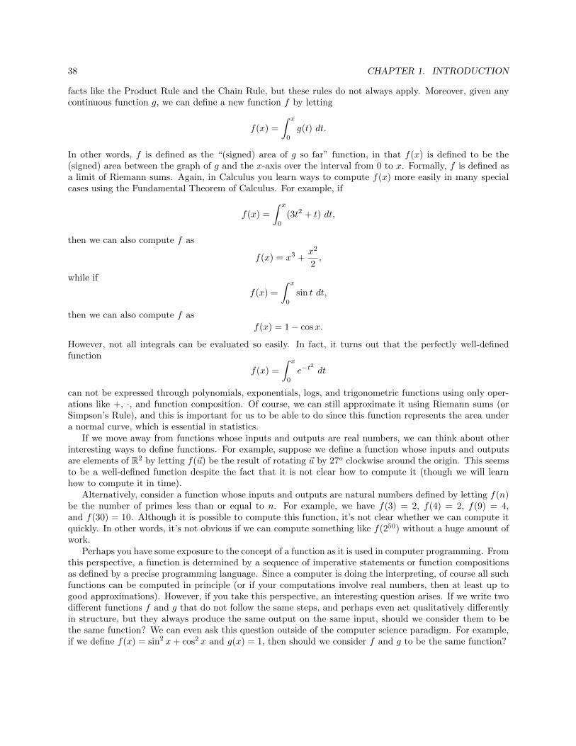
38 CHAPTER 1. INTRODUCTION
facts like the Product Rule and the Chain Rule, but these rules do not always apply. Moreover, given anycontinuous function g, we can define a new function f by letting
f(x) =
∫ x
0
g(t) dt.
In other words, f is defined as the “(signed) area of g so far” function, in that f(x) is defined to be the(signed) area between the graph of g and the x-axis over the interval from 0 to x. Formally, f is defined asa limit of Riemann sums. Again, in Calculus you learn ways to compute f(x) more easily in many specialcases using the Fundamental Theorem of Calculus. For example, if
f(x) =
∫ x
0
(3t2 + t) dt,
then we can also compute f as
f(x) = x3 +x2
2,
while if
f(x) =
∫ x
0
sin t dt,
then we can also compute f as
f(x) = 1− cosx.
However, not all integrals can be evaluated so easily. In fact, it turns out that the perfectly well-definedfunction
f(x) =
∫ x
0
e−t2
dt
can not be expressed through polynomials, exponentials, logs, and trigonometric functions using only oper-ations like +, ·, and function composition. Of course, we can still approximate it using Riemann sums (orSimpson’s Rule), and this is important for us to be able to do since this function represents the area undera normal curve, which is essential in statistics.
If we move away from functions whose inputs and outputs are real numbers, we can think about otherinteresting ways to define functions. For example, suppose we define a function whose inputs and outputsare elements of R2 by letting f(~u) be the result of rotating ~u by 27o clockwise around the origin. This seemsto be a well-defined function despite the fact that it is not clear how to compute it (though we will learnhow to compute it in time).
Alternatively, consider a function whose inputs and outputs are natural numbers defined by letting f(n)be the number of primes less than or equal to n. For example, we have f(3) = 2, f(4) = 2, f(9) = 4,and f(30) = 10. Although it is possible to compute this function, it’s not clear whether we can compute itquickly. In other words, it’s not obvious if we can compute something like f(250) without a huge amount ofwork.
Perhaps you have some exposure to the concept of a function as it is used in computer programming. Fromthis perspective, a function is determined by a sequence of imperative statements or function compositionsas defined by a precise programming language. Since a computer is doing the interpreting, of course all suchfunctions can be computed in principle (or if your computations involve real numbers, then at least up togood approximations). However, if you take this perspective, an interesting question arises. If we write twodifferent functions f and g that do not follow the same steps, and perhaps even act qualitatively differentlyin structure, but they always produce the same output on the same input, should we consider them to bethe same function? We can even ask this question outside of the computer science paradigm. For example,if we define f(x) = sin2 x+ cos2 x and g(x) = 1, then should we consider f and g to be the same function?
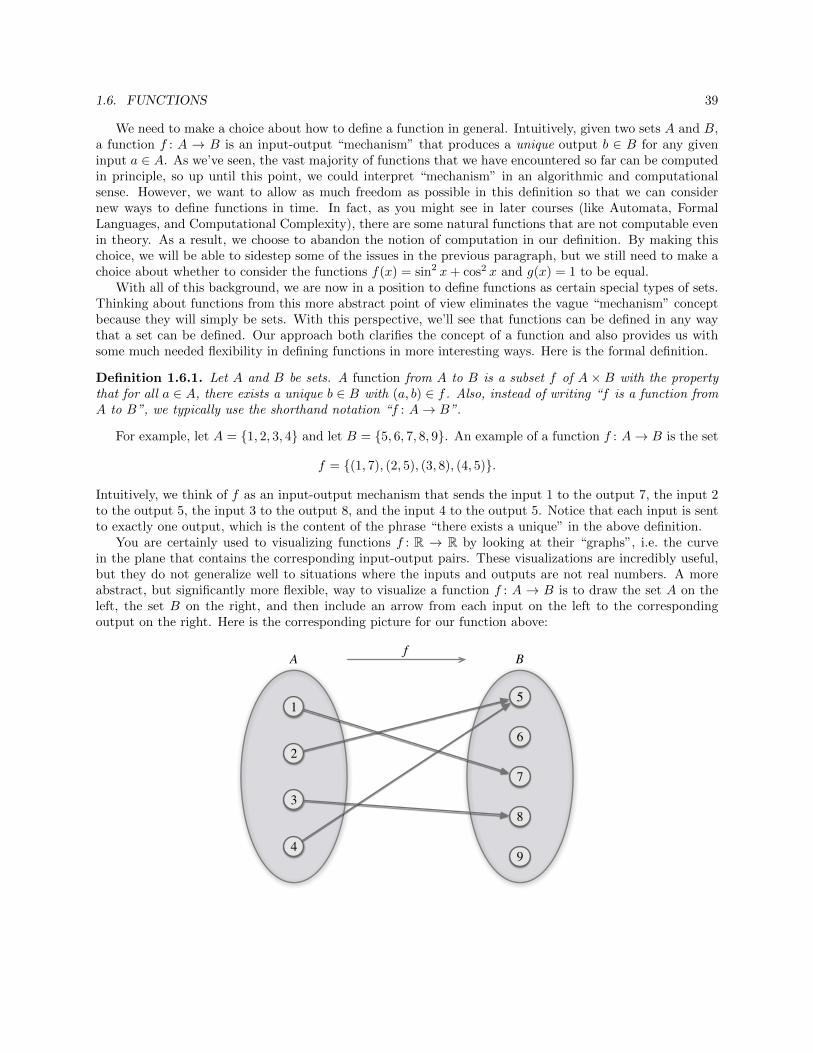
1.6. FUNCTIONS 39
We need to make a choice about how to define a function in general. Intuitively, given two sets A and B,a function f : A → B is an input-output “mechanism” that produces a unique output b ∈ B for any giveninput a ∈ A. As we’ve seen, the vast majority of functions that we have encountered so far can be computedin principle, so up until this point, we could interpret “mechanism” in an algorithmic and computationalsense. However, we want to allow as much freedom as possible in this definition so that we can considernew ways to define functions in time. In fact, as you might see in later courses (like Automata, FormalLanguages, and Computational Complexity), there are some natural functions that are not computable evenin theory. As a result, we choose to abandon the notion of computation in our definition. By making thischoice, we will be able to sidestep some of the issues in the previous paragraph, but we still need to make achoice about whether to consider the functions f(x) = sin2 x+ cos2 x and g(x) = 1 to be equal.
With all of this background, we are now in a position to define functions as certain special types of sets.Thinking about functions from this more abstract point of view eliminates the vague “mechanism” conceptbecause they will simply be sets. With this perspective, we’ll see that functions can be defined in any waythat a set can be defined. Our approach both clarifies the concept of a function and also provides us withsome much needed flexibility in defining functions in more interesting ways. Here is the formal definition.
Definition 1.6.1. Let A and B be sets. A function from A to B is a subset f of A × B with the propertythat for all a ∈ A, there exists a unique b ∈ B with (a, b) ∈ f . Also, instead of writing “f is a function fromA to B”, we typically use the shorthand notation “f : A→ B”.
For example, let A = {1, 2, 3, 4} and let B = {5, 6, 7, 8, 9}. An example of a function f : A→ B is the set
f = {(1, 7), (2, 5), (3, 8), (4, 5)}.
Intuitively, we think of f as an input-output mechanism that sends the input 1 to the output 7, the input 2to the output 5, the input 3 to the output 8, and the input 4 to the output 5. Notice that each input is sentto exactly one output, which is the content of the phrase “there exists a unique” in the above definition.
You are certainly used to visualizing functions f : R → R by looking at their “graphs”, i.e. the curvein the plane that contains the corresponding input-output pairs. These visualizations are incredibly useful,but they do not generalize well to situations where the inputs and outputs are not real numbers. A moreabstract, but significantly more flexible, way to visualize a function f : A → B is to draw the set A on theleft, the set B on the right, and then include an arrow from each input on the left to the correspondingoutput on the right. Here is the corresponding picture for our function above:
fBA
9
8
7
6
5
4
3
2
1
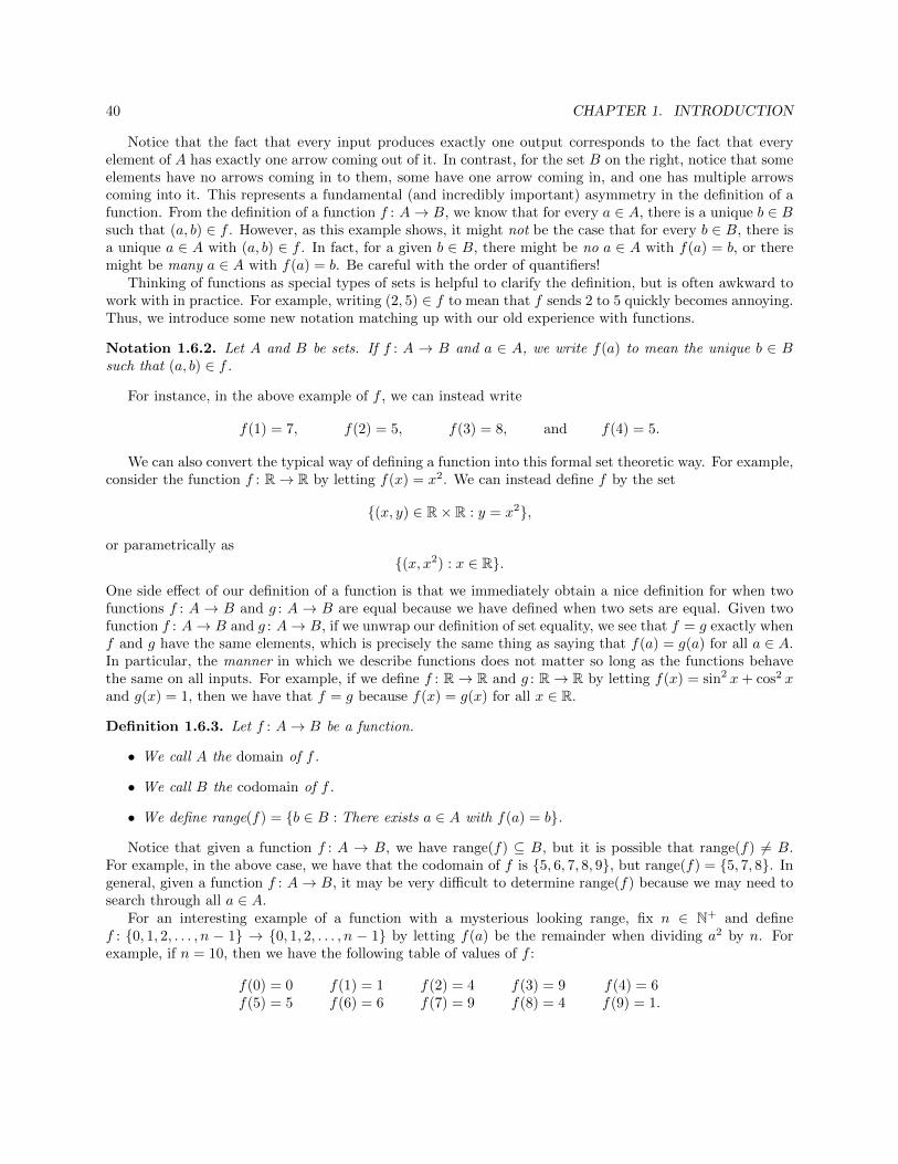
40 CHAPTER 1. INTRODUCTION
Notice that the fact that every input produces exactly one output corresponds to the fact that everyelement of A has exactly one arrow coming out of it. In contrast, for the set B on the right, notice that someelements have no arrows coming in to them, some have one arrow coming in, and one has multiple arrowscoming into it. This represents a fundamental (and incredibly important) asymmetry in the definition of afunction. From the definition of a function f : A→ B, we know that for every a ∈ A, there is a unique b ∈ Bsuch that (a, b) ∈ f . However, as this example shows, it might not be the case that for every b ∈ B, there isa unique a ∈ A with (a, b) ∈ f . In fact, for a given b ∈ B, there might be no a ∈ A with f(a) = b, or theremight be many a ∈ A with f(a) = b. Be careful with the order of quantifiers!
Thinking of functions as special types of sets is helpful to clarify the definition, but is often awkward towork with in practice. For example, writing (2, 5) ∈ f to mean that f sends 2 to 5 quickly becomes annoying.Thus, we introduce some new notation matching up with our old experience with functions.
Notation 1.6.2. Let A and B be sets. If f : A → B and a ∈ A, we write f(a) to mean the unique b ∈ Bsuch that (a, b) ∈ f .
For instance, in the above example of f , we can instead write
f(1) = 7, f(2) = 5, f(3) = 8, and f(4) = 5.
We can also convert the typical way of defining a function into this formal set theoretic way. For example,consider the function f : R→ R by letting f(x) = x2. We can instead define f by the set
{(x, y) ∈ R× R : y = x2},
or parametrically as
{(x, x2) : x ∈ R}.
One side effect of our definition of a function is that we immediately obtain a nice definition for when twofunctions f : A → B and g : A → B are equal because we have defined when two sets are equal. Given twofunction f : A→ B and g : A→ B, if we unwrap our definition of set equality, we see that f = g exactly whenf and g have the same elements, which is precisely the same thing as saying that f(a) = g(a) for all a ∈ A.In particular, the manner in which we describe functions does not matter so long as the functions behavethe same on all inputs. For example, if we define f : R→ R and g : R→ R by letting f(x) = sin2 x+ cos2 xand g(x) = 1, then we have that f = g because f(x) = g(x) for all x ∈ R.
Definition 1.6.3. Let f : A→ B be a function.
• We call A the domain of f .
• We call B the codomain of f .
• We define range(f) = {b ∈ B : There exists a ∈ A with f(a) = b}.
Notice that given a function f : A → B, we have range(f) ⊆ B, but it is possible that range(f) 6= B.For example, in the above case, we have that the codomain of f is {5, 6, 7, 8, 9}, but range(f) = {5, 7, 8}. Ingeneral, given a function f : A→ B, it may be very difficult to determine range(f) because we may need tosearch through all a ∈ A.
For an interesting example of a function with a mysterious looking range, fix n ∈ N+ and definef : {0, 1, 2, . . . , n − 1} → {0, 1, 2, . . . , n − 1} by letting f(a) be the remainder when dividing a2 by n. Forexample, if n = 10, then we have the following table of values of f :
f(0) = 0 f(1) = 1 f(2) = 4 f(3) = 9 f(4) = 6f(5) = 5 f(6) = 6 f(7) = 9 f(8) = 4 f(9) = 1.
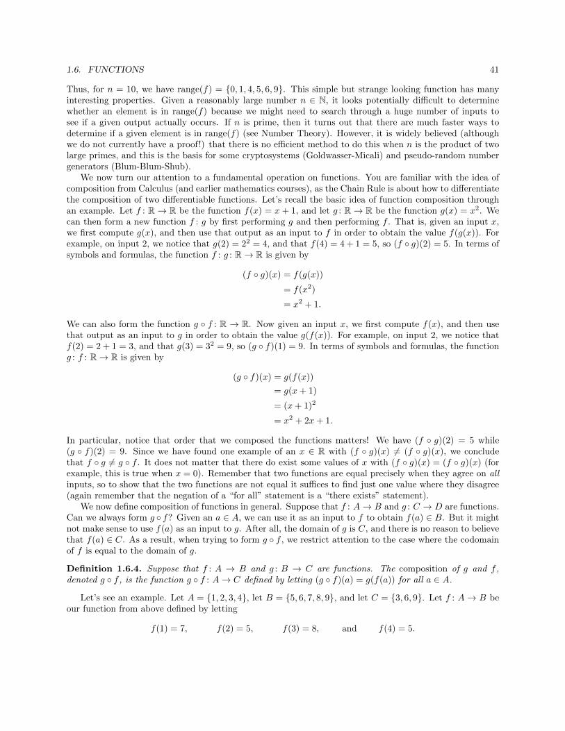
1.6. FUNCTIONS 41
Thus, for n = 10, we have range(f) = {0, 1, 4, 5, 6, 9}. This simple but strange looking function has manyinteresting properties. Given a reasonably large number n ∈ N, it looks potentially difficult to determinewhether an element is in range(f) because we might need to search through a huge number of inputs tosee if a given output actually occurs. If n is prime, then it turns out that there are much faster ways todetermine if a given element is in range(f) (see Number Theory). However, it is widely believed (althoughwe do not currently have a proof!) that there is no efficient method to do this when n is the product of twolarge primes, and this is the basis for some cryptosystems (Goldwasser-Micali) and pseudo-random numbergenerators (Blum-Blum-Shub).
We now turn our attention to a fundamental operation on functions. You are familiar with the idea ofcomposition from Calculus (and earlier mathematics courses), as the Chain Rule is about how to differentiatethe composition of two differentiable functions. Let’s recall the basic idea of function composition throughan example. Let f : R→ R be the function f(x) = x+ 1, and let g : R→ R be the function g(x) = x2. Wecan then form a new function f : g by first performing g and then performing f . That is, given an input x,we first compute g(x), and then use that output as an input to f in order to obtain the value f(g(x)). Forexample, on input 2, we notice that g(2) = 22 = 4, and that f(4) = 4 + 1 = 5, so (f ◦ g)(2) = 5. In terms ofsymbols and formulas, the function f : g : R→ R is given by
(f ◦ g)(x) = f(g(x))
= f(x2)
= x2 + 1.
We can also form the function g ◦ f : R → R. Now given an input x, we first compute f(x), and then usethat output as an input to g in order to obtain the value g(f(x)). For example, on input 2, we notice thatf(2) = 2 + 1 = 3, and that g(3) = 32 = 9, so (g ◦ f)(1) = 9. In terms of symbols and formulas, the functiong : f : R→ R is given by
(g ◦ f)(x) = g(f(x))
= g(x+ 1)
= (x+ 1)2
= x2 + 2x+ 1.
In particular, notice that order that we composed the functions matters! We have (f ◦ g)(2) = 5 while(g ◦ f)(2) = 9. Since we have found one example of an x ∈ R with (f ◦ g)(x) 6= (f ◦ g)(x), we concludethat f ◦ g 6= g ◦ f . It does not matter that there do exist some values of x with (f ◦ g)(x) = (f ◦ g)(x) (forexample, this is true when x = 0). Remember that two functions are equal precisely when they agree on allinputs, so to show that the two functions are not equal it suffices to find just one value where they disagree(again remember that the negation of a “for all” statement is a “there exists” statement).
We now define composition of functions in general. Suppose that f : A→ B and g : C → D are functions.Can we always form g ◦ f? Given an a ∈ A, we can use it as an input to f to obtain f(a) ∈ B. But it mightnot make sense to use f(a) as an input to g. After all, the domain of g is C, and there is no reason to believethat f(a) ∈ C. As a result, when trying to form g ◦ f , we restrict attention to the case where the codomainof f is equal to the domain of g.
Definition 1.6.4. Suppose that f : A → B and g : B → C are functions. The composition of g and f ,denoted g ◦ f , is the function g ◦ f : A→ C defined by letting (g ◦ f)(a) = g(f(a)) for all a ∈ A.
Let’s see an example. Let A = {1, 2, 3, 4}, let B = {5, 6, 7, 8, 9}, and let C = {3, 6, 9}. Let f : A→ B beour function from above defined by letting
f(1) = 7, f(2) = 5, f(3) = 8, and f(4) = 5.
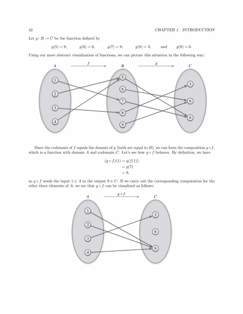
42 CHAPTER 1. INTRODUCTION
Let g : B → C be the function defined by
g(5) = 9, g(6) = 6, g(7) = 9, g(8) = 3, and g(9) = 6.
Using our more abstract visualization of functions, we can picture this situation in the following way:
gfCBA
9
6
3
9
8
7
6
5
4
3
2
1
Since the codomain of f equals the domain of g (both are equal to B), we can form the composition g ◦f ,which is a function with domain A and codomain C. Let’s see how g ◦ f behaves. By definition, we have
(g ◦ f)(1) = g(f(1))
= g(7)
= 9,
so g ◦ f sends the input 1 ∈ A to the output 9 ∈ C. If we carry out the corresponding computation for theother three elements of A, we see that g ◦ f can be visualized as follows:
g f CA
9
6
3
4
3
2
1
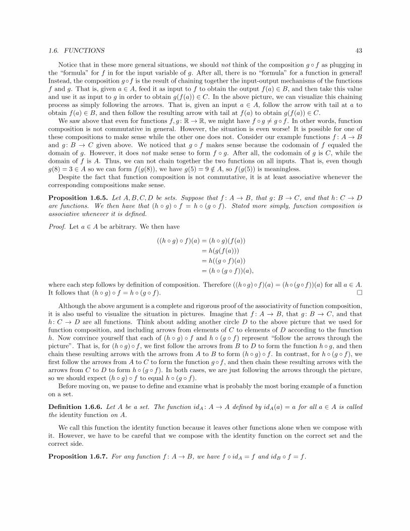
1.6. FUNCTIONS 43
Notice that in these more general situations, we should not think of the composition g ◦ f as plugging inthe “formula” for f in for the input variable of g. After all, there is no “formula” for a function in general!Instead, the composition g◦f is the result of chaining together the input-output mechanisms of the functionsf and g. That is, given a ∈ A, feed it as input to f to obtain the output f(a) ∈ B, and then take this valueand use it as input to g in order to obtain g(f(a)) ∈ C. In the above picture, we can visualize this chainingprocess as simply following the arrows. That is, given an input a ∈ A, follow the arrow with tail at a toobtain f(a) ∈ B, and then follow the resulting arrow with tail at f(a) to obtain g(f(a)) ∈ C.
We saw above that even for functions f, g : R→ R, we might have f ◦ g 6= g ◦ f . In other words, functioncomposition is not commutative in general. However, the situation is even worse! It is possible for one ofthese compositions to make sense while the other one does not. Consider our example functions f : A→ Band g : B → C given above. We noticed that g ◦ f makes sense because the codomain of f equaled thedomain of g. However, it does not make sense to form f ◦ g. After all, the codomain of g is C, while thedomain of f is A. Thus, we can not chain together the two functions on all inputs. That is, even thoughg(8) = 3 ∈ A so we can form f(g(8)), we have g(5) = 9 /∈ A, so f(g(5)) is meaningless.
Despite the fact that function composition is not commutative, it is at least associative whenever thecorresponding compositions make sense.
Proposition 1.6.5. Let A,B,C,D be sets. Suppose that f : A → B, that g : B → C, and that h : C → Dare functions. We then have that (h ◦ g) ◦ f = h ◦ (g ◦ f). Stated more simply, function composition isassociative whenever it is defined.
Proof. Let a ∈ A be arbitrary. We then have
((h ◦ g) ◦ f)(a) = (h ◦ g)(f(a))
= h(g(f(a)))
= h((g ◦ f)(a))
= (h ◦ (g ◦ f))(a),
where each step follows by definition of composition. Therefore ((h◦g)◦f)(a) = (h◦ (g ◦f))(a) for all a ∈ A.It follows that (h ◦ g) ◦ f = h ◦ (g ◦ f).
Although the above argument is a complete and rigorous proof of the associativity of function composition,it is also useful to visualize the situation in pictures. Imagine that f : A → B, that g : B → C, and thath : C → D are all functions. Think about adding another circle D to the above picture that we used forfunction composition, and including arrows from elements of C to elements of D according to the functionh. Now convince yourself that each of (h ◦ g) ◦ f and h ◦ (g ◦ f) represent “follow the arrows through thepicture”. That is, for (h ◦ g) ◦ f , we first follow the arrows from B to D to form the function h ◦ g, and thenchain these resulting arrows with the arrows from A to B to form (h ◦ g) ◦ f . In contrast, for h ◦ (g ◦ f), wefirst follow the arrows from A to C to form the function g ◦f , and then chain these resulting arrows with thearrows from C to D to form h ◦ (g ◦ f). In both cases, we are just following the arrows through the picture,so we should expect (h ◦ g) ◦ f to equal h ◦ (g ◦ f).
Before moving on, we pause to define and examine what is probably the most boring example of a functionon a set.
Definition 1.6.6. Let A be a set. The function idA : A → A defined by idA(a) = a for all a ∈ A is calledthe identity function on A.
We call this function the identity function because it leaves other functions alone when we compose withit. However, we have to be careful that we compose with the identity function on the correct set and thecorrect side.
Proposition 1.6.7. For any function f : A→ B, we have f ◦ idA = f and idB ◦ f = f .
44 CHAPTER 1. INTRODUCTION
Proof. Let f : A→ B be an arbitrary function.
• We first show that f ◦ idA = f . Let a ∈ A be arbitrary. We have
(f ◦ idA)(a) = f(idA(a)) (by definition of composition)
= f(a)
Since a ∈ A was arbitrary, it follows that f ◦ idA = f .
• We now show that idB ◦ f = f . Let a ∈ A be arbitrary. We have
(idB ◦ f)(a) = idB(f(a)) (by definition of composition)
= f(a) (because f(a) ∈ B)
Since a ∈ A was arbitrary, it follows that idB ◦ f = f .
1.7 Injective, Surjective, and Bijective Functions
Recall that the key property in the definition of a function f : A → B is that every input element from Aproduces a unique output element from B. However, this does not work in reverse. Given b ∈ B, it may bethe case that b is the output of zero, one, or many elements from A. We give special names to the types offunctions that have limitations on how often each element of B actually occurs as an output.
Definition 1.7.1. Let f : A→ B be a function.
• We say that f is injective (or one-to-one) if whenever a1, a2 ∈ A satisfy f(a1) = f(a2), we havea1 = a2.
• We say that f is surjective (or onto) if for all b ∈ B, there exists a ∈ A such that f(a) = b.
• We say that f is bijective if f is both injective and surjective.
Let’s take a moment to unpack these definitions. First, saying that a function f : A→ B is surjective issimply saying that every b ∈ B is hit at least once by an element a ∈ A. In terms of our above visualizations,a function f : A → B is surjective if every element of B has at least one arrow coming in to it. We canrephrase this idea using Definition 1.6.3 by saying that f : A→ B is surjective exactly when range(f) = B.
The definition of injective is slightly more mysterious at first. Intuitively, a function f : A→ B is injectivewhen every b ∈ B is hit by at most one a ∈ A, i.e. if every element of B has at most one arrow coming intoit. Now saying this precisely takes a little bit of thought. After all, it is difficult to say “there exists at mostone” because our “there exists” quantifier is used to mean that there is at least one! The idea is to turnthis around and not directly talk about b ∈ B at all. Instead, we want to say that we never have a situationwhere we have two distinct elements a1, a2 ∈ A that go to the same place under f . Thus, we want to say
“Not(There exists a1, a2 ∈ A with a1 6= a2 and f(a1) = f(a2))”.
We can rewrite this statement as
“For all a1, a2 ∈ A, we have Not(a1 6= a2 and f(a1) = f(a2))”,
which is equivalent to
“For all a1, a2 ∈ A, we have either a1 = a2 or f(a1) 6= f(a2)”
1.7. INJECTIVE, SURJECTIVE, AND BIJECTIVE FUNCTIONS 45
(notice that the negation of the “and” statement became an “or” statement). Finally, we can rewrite thisas the following “if...then...” statement:
“For all a1, a2 ∈ A, if a1 6= a2, then f(a1) 6= f(a2)”.
Looking at our statement here, it captures what we want to express perfectly because it says that distinctinputs always go to distinct outputs, which exactly says no element of B is hit by 2 or more elements, andhence that every element of B is hit by at most 1 element. Thus, we could indeed take this as our definitionof injective. The problem is that this definition is difficult to use in practice. To see why, think about howwe would argue that a given function f : A→ B is injective. It appears that we would want to take arbitrarya1, a2 ∈ A with a1 6= a2, and argue that under this assumption we must have that f(a1) 6= f(a2). Nowthe problem with this is that is very difficult to work with an expression involving 6= in ways that preservetruth. For example, we have that −1 6= 1, but (−1)2 = 12, so we can not square both sides and preservenon-equality. To get around this problem, we instead take the contrapositive of the statement in question,which turns into our formal definition of injective:
“For all a1, a2 ∈ A, if f(a1) = f(a2), then a1 = a2”.
Notice that in our definition above, we simply replace the “for all... if... then...” construct with a “when-ever...we have...” for clarity, but these are saying precisely the same thing, i.e. that whenever we have twoelements of A that happen to be sent to the same element of B, then in fact those two elements of A mustbe the same. Although our official definition is slightly harder to wrap one’s mind around, it is much easierto work with in practice. To prove that a given f : A → B is injective, we take arbitrary a1, a2 ∈ A withf(a1) = f(a2), and use this equality to derive the conclusion that a1 = a2.
To recap the colloquial ways to understand these concepts, a function f : A → B is injective if everyb ∈ B is hit by at most one a ∈ A, and is surjective if every b ∈ B is hit by at least one a ∈ A. It followsthat a function f : A → B is bijective if every b ∈ B is hit by exactly one a ∈ A. These ways of thinkingabout injective and surjective are great, but we need to be careful when proving that a function is injectiveor surjective. Given a function f : A→ B, here is the general process for proving that it has one or both ofthese properties:
• Suppose we want to prove that a function f : A→ B is injective. Notice that the definition involves a“for all” quantifier. Thus, we should start by taking arbitrary a1, a2 ∈ A that satisfy f(a1) = f(a2),and then work forward to derive that a1 = a2. In this way, we show that whenever two elements of Ahappen to produce the same output, then they must have been the same element all along.
• Suppose we want to prove that a function f : A→ B is surjective. Notice that the definition is a “forall. . . there exists. . . ” statement. Thus, we should start by taking an arbitrary b ∈ B, and then showhow to build an a ∈ A with f(a) = b. In other words, we need to take an arbitrary b ∈ B and fill inthe blank in f( ) = b with an element of A.
Here is an example.
Proposition 1.7.2. The function f : R→ R given by f(x) = 5x− 7 is bijective.
Proof. We need to show that f is both injective and surjective.
• We first show that f is injective. Let x1, x2 ∈ R be arbitrary with f(x1) = f(x2). By definition of f ,we then have that 5x1 − 7 = 5x2 − 7. Adding 7 to both sides, we see that 5x1 = 5x2. Dividing bothsides by 5, we conclude that x1 = x2. Therefore, f is injective.
46 CHAPTER 1. INTRODUCTION
• We next show that f is surjective. Let y ∈ R be arbitrary. Notice that y+75 ∈ R and that
f
(y + 7
5
)= 5 · y + 7
5− 7
= (y + 7)− 7
= y.
Thus, we have shown the existence of an x ∈ R with f(x) = y. Therefore, f is surjective.
Since f is both injective and surjective, it follows that f is bijective.
Here’s another example. In this case, we show that a function is not surjective. Let’s think the logichere. Given a function f : A→ B, the statement that f is surjective is:
“For all b ∈ B, there exists a ∈ A such that f(a) = b”.
Saying that a function f : A→ B is not surjective is saying that the negation of this statement is true. Nowwe can express the negation of this statement as follows:
“There exists b ∈ B such that for all a ∈ A, we have f(a) 6= b”.
Thus, to argue that a function f : A→ B is not surjective, we have to give an example of an element b ∈ Bthat is not hit by any a ∈ A.
Proposition 1.7.3. The function f : Z→ Z given by f(n) = 2n is injective but not surjective.
Proof. We show each part:
• We first show that f is injective. Let n1, n2 ∈ Z be arbitrary with f(n1) = f(n2). By definition of f ,we then have that 2n1 = 2n2. Dividing both sides by 2, we conclude that n1 = n2. Therefore, f isinjective.
• We next show that f is not surjective. We claim that 1 ∈ Z has the property that f(n) 6= 1 for alln ∈ Z. To see this, suppose instead that there does exist an n ∈ Z with f(n) = 1, and fix such an n.We would then have that 2n = 1, so 1 would be even, which contradicts Proposition 1.4.4. It followsthat f(n) 6= 1 for all n ∈ Z, and hence f is not surjective.
Notice that if we define g : R → R by letting g(x) = 2x, then g is injective by the same proof, butg is surjective (think about why). Thus, changing the domain or codomain of a function can change theproperties of that function. We will have much more to say about injective and surjective functions in time.
Given a general function f : A → B, we’ve seen that every element of A produces a unique element ofB (by the definition of a function), but it might not be the case that every element of B is hit by a uniqueelement of A. Thus, there is a serious asymmetry between the domain and the codomain. In particular, wecan not typically “undo” a function. That is, if we have a function f : A → B together with a particularb ∈ B, we can not generally go backwards and produce the unique element of A that hits it. After all, if agiven b ∈ B is not in range(f), then there is no natural candidate element of A, and if b ∈ B is in range(f),then there might be several candidates.
Now if f : A→ B is a bijection, then all of these problems go away, because then every b ∈ B is hit by aunique a ∈ A. In this setting, we can define a “backwards” function g : B → A by just reversing the arrows.The resulting function is naturally called the inverse of f . Here is the formal definition.
Definition 1.7.4. Let f : A→ B be a bijective function. We define a new function f−1 : B → A as follows.Given b ∈ B, let f−1(b) be the unique a ∈ A that satisfies f(a) = b.
1.7. INJECTIVE, SURJECTIVE, AND BIJECTIVE FUNCTIONS 47
At first, this definition might look strange, because f−1 is defined in a wordy way without informationabout how to “compute” it. However, remember that a function need not be given by a formula! For anyb ∈ B, we have identified a unique element of A to assign to the value f−1(b), and that is all we need to doto define a function.
For example, consider A = {1, 2, 3} and B = {4, 5, 6}. Define f : A→ B as follows:
f(1) = 6, f(2) = 5, and f(3) = 4.
Notice that f is bijective, so f−1 is defined as a function with domain B and codomain A. What is f−1(4)?Looking at the definition, we need to find the unique a ∈ A with f(a) = 4. In this case, the unique suchvalue is 3, so f−1(4) = 3. Working through the other values, we determine the following:
f−1(4) = 3, f−1(5) = 2, and f−1(6) = 1.
Here is another way to think about the inverse function in terms of sets. As a set, we have
f = {(1, 6), (2, 5), (3, 4)}.
Notice thatf−1 = {(4, 3), (5, 2), (6, 1)},
which is the just the result of flipping each of the ordered pairs in f . In general, if you choose to view afunction f : A→ B as the corresponding set of ordered pairs, then
f−1 = {(b, a) ∈ B ×A : (a, b) ∈ f}.
Although this a clever set-theoretic way to think about f−1, and it feels closer to the “flipping the arrows”intuition, it is a bit abstract and typically not as useful when the domain or codomain are infinite.
Let’s see how this works in a context where the domain and codomain are infinite. As mentioned in Section1.6, given x ≥ 0 we typically think of
√x as the unique y ≥ 0 with the property that y2 = x. That’s a wordy
definition that looks like an inverse! To explore this idea, we start by looking at the function g : R → Rdefined by g(x) = x2. Unfortunately, g is not bijective. It is not injective because g(1) = 1 = g(−1), but1 6= −1. Also, it is not surjective because −1 /∈ range(g).
Let’s fix this issue by changing the domain and codomain. Let A = {x ∈ R : x ≥ 0} be the set ofnonnegative real numbers. Now define f : A → A by letting f(x) = x2. It is possible to show that f isbijective (one uses the fact that f is increasing to show that f is injective, and the Intermediate ValueTheorem from Analysis to argue that f is surjective). Thus, f−1 is defined as a function with domain A andcodomain A, i.e. we have a function f−1 : A→ A. By definition, given x ∈ A, we have defined f−1(x) to bebe the unique y ∈ A that satisfies f(y) = x. That is, for any x ≥ 0, we have that f−1(x) is the unique y ≥ 0that satisfies y2 = x. In other words, the square root function is really defined as an inverse! Similarly, if wedefine h : R→ {x ∈ R : x > 0} by letting h(x) = ex, then h is bijective, and so has an inverse. We call thisinverse function the natural log.
Before moving on, we discuss one other abstract but powerful way to think about inverse functions. Letf : A → B be a bijective function. We then have an inverse function f−1 : B → A. Can we compose thesetwo functions? Notice that the codomain of f equals the domain of f−1 (both are B), so we can formf−1 ◦ f , and this function has domain A and codomain A. That is, we have f−1 ◦ f : A → A. What isthis composition? Intuitively, given any a ∈ A, we first feed the input a into f and follow the arrow to getf(a) ∈ B, and then feed this result into f−1 to go back across the arrow to arrive back at a. In other words,it seems that we should have f−1(f(a)) = a for all a ∈ A. We can also compose the functions in the otherorder, but notice now that f ◦f−1 : B → B. A similar argument suggests that we should have f(f−1(b)) = bfor all b ∈ B. We now verify these suspicions carefully.
Proposition 1.7.5. Let f : A→ B be a bijective function.
48 CHAPTER 1. INTRODUCTION
1. For all a ∈ A, we have f−1(f(a)) = a. Thus, f−1 ◦ f = idA.
2. For all b ∈ B, we have f(f−1(b)) = b. Thus, f ◦ f−1 = idB.
Proof.
1. Let a ∈ A be arbitrary. By definition of the inverse function f−1(f(a)) is defined to be the uniquec ∈ A such that f(c) = f(a). But of course a is an example of such an element of A, as we triviallyhave f(a) = f(a). Thus, we must have f−1(f(a)) = a.
We now show that f−1 ◦ f = idA. Let a ∈ A be arbitrary. We have
(f−1 ◦ f)(a) = f−1(f(a)) (by definition of composition)
= a (from above)
= idA(a) (by definition of idA).
Since a ∈ A was arbitrary, we conclude that f−1 ◦ f = idA.
2. Let b ∈ B be arbitrary. By definition of the inverse function, we know that f−1(b) is the unique a ∈ Athat satisfies f(a) = b. Thus, we must have f(f−1(b)) = b.
We now show that f ◦ f−1 = idB . Let b ∈ B be arbitrary. We have
(f ◦ f−1)(b) = f(f−1(b)) (by definition of composition)
= b (from above)
= idB(b) (by definition of idB).
Since b ∈ B was arbitrary, we conclude that f ◦ f−1 = idB .
1.8 Solving Equations
Suppose that we want to solve the equation 3x−7 = 4 in R. In other words, we want to find all real numberssuch that when we plug them in for x, the result in a true statement. Of course, we can naturally follow theprocedures from algebra. Thus, we add 7 to both sides to conclude that 3x = 11, and then divide both sidesby 3 to conclude that x = 11
3 . The idea of this process is to preform the same operation to both sides in aneffort to isolate x.
That all sounds good, but now suppose that we try to solve the equation x− 2 = 1 in R. Maybe we didnot think to add 2 to both sides, and instead decide to square both sides because we like quadratics. Wethen arrive at (x−2)2 = 12, so x2−4x+4 = 1. Now we remember to subtract 1 from both sides to concludethat x2−4x+ 3 = 0, and hence (x−3)(x−1) = 0. It follows that x = 3 and x = 1 are both solutions, right?Right? Of course, 1 is not actually a solution to x− 2 = 1, but it may not be obvious what went wrong. Inorder to understand what is happening here, we need to think about the logic of what we are doing whenwe blindly apply this “do the same thing to both sides” procedure.
Let’s start to think through the logic of solving equations carefully. We want to find all x ∈ R such thatx− 2 = 1 is true. The idea then is to assume that we have a real number that gives a true statement whenwe plug it in, and then see what we can say about that real number. Let’s formalize this a bit by giving thereal number a name. Assume that we have an a ∈ R such that a− 2 = 1 is true. Now we have an actual realnumber a in hand and it has the property that a−2 equals the same thing as 1. Since these two real numbersa−2 and 1 are the same real number, we can then conclude that (a−2)2 = 12 because we’ve simply squaredthe same real number. We now do algebra to conclude that a2 − 4a+ 4 = 1. Since these two real numbers
1.8. SOLVING EQUATIONS 49
a2 − 4a + 4 and 1 are the same real number, if we subtract one from both of them, then the resulting tworeal numbers are equal. Thus, we can conclude that a2 − 4a+ 3 = 0. Since (a− 3)(a− 1) = a2 + 4a+ 3 (byusing the Distributive Law twice), we can conclude that (a − 3)(a − 1) = 0. Now we use the fundamentalfact that if the product of two real numbers is 0, then one of the two numbers must be 0, so we can concludethat either a− 3 = 0 or a− 1 = 0. By adding the same thing to both sides of each of these, it follows thata = 3 or a = 1.
Did you follow all of that logic? If so, the only conclusion that we can draw is that if a ∈ R is such thata − 2 = 1, then it must be the case that either a = 3 or a = 1. Notice that the logic flows forward, whichis why we can only conclude that an “if...then...” statement is true. The logic of the argument says nothingabout the converse of this “if...then...”. In other words, there is no reason to believe that the statement “ifeither a = 3 or a = 1, then a− 2 = 1” is true, and in fact it is false! In general, all that we can say is thatif we perform an operation on both sides of an equality, then elements that made the original equation truewill make the resulting equation true.
Let’s formalize all of this in a definition. To talk about an “equation”, we are really talking about thetwo functions on each side of the equation. For example, asking for those x ∈ R such that 3x − 7 = 4 isasking the following question: If f : R→ R is f(x) = 3x− 7, and g : R→ R is g(x) = 4, then determine thevalues a ∈ R such that f(a) = g(a) is true. We give this collection of values a special name.
Definition 1.8.1. Suppose that we have two functions f : A → B and g : A → B. We define the solutionset of the equation f(x) = g(x) to be {a ∈ A : f(a) = g(a)}.
Of course, the question we have to ask ourselves is how we determine the solution set of a given equation.In general, this is a hard problem. However, the techniques of algebra encourage us to perform the sameoperations on both sides of the equality with the hopes of isolating x. Suppose that we have two functionsf : A → B and g : A → B, and we let S be the solution set of the equation f(x) = g(x). Suppose that weperform an operation on both sides of this equality, and we let T be the solution set of the resulting equation.By the arguments and examples given at the beginning of this section, we see that S ⊆ T , but it is possiblethat T 6⊆ S in general! However, if we are able to determine T , we can always go back and plug all of thesevalues of T into the equation to determine which of them are in S.
Consider the following examples:
• If f : R → R is f(x) = 3x − 7, and g : R → R is g(x) = 4, then the solution set of the equationf(x) = g(x) is { 113 }.
• If f : R → R is f(x) = x2, and g : R → R is g(x) = 7x − 12, then the solution set of the equationf(x) = g(x) is {3, 4}.
• If f : R → R is f(x) = x, and g : R → R is g(x) = x + 1, then the solution set of the equationf(x) = g(x) is ∅.
• If f : R → R is f(x) = sinx, and g : R → R is g(x) = cosx, then the solution set of the equationf(x) = g(x) is {π4 + πn : n ∈ Z}.
As these examples illustrate, the solution set of an equation can have 1 element, no elements, several ele-ments, or infinitely many elements.
We can also consider equations with many variables, such as x+2y = 1 where the variables range over R.We can try to generalize the above definition, but in fact this is not necessary. We can instead consider thetwo sides of the equation as functions of two variables. Thus, we are considering the functions f : R2 → Rgiven by f((x, y)) = x + 2y and g : R2 → R given by g((x, y)) = 1. To determine the solution set, we justneed to find those elements in R2 that make the equation true, i.e. we need to find the solution set S. Ofcourse, one way to describe S is simply as
S = {(x, y) ∈ R2 : x+ 2y = 1}.
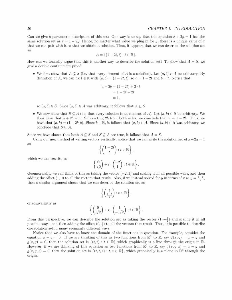
50 CHAPTER 1. INTRODUCTION
Can we give a parametric description of this set? One way is to say that the equation x + 2y = 1 has thesame solution set as x = 1− 2y. Hence, no matter what value we plug in for y, there is a unique value of xthat we can pair with it so that we obtain a solution. Thus, it appears that we can describe the solution setas
A = {(1− 2t, t) : t ∈ R}.
How can we formally argue that this is another way to describe the solution set? To show that A = S, wegive a double containment proof:
• We first show that A ⊆ S (i.e. that every element of A is a solution). Let (a, b) ∈ A be arbitrary. Bydefinition of A, we can fix t ∈ R with (a, b) = (1− 2t, t), so a = 1− 2t and b = t. Notice that
a+ 2b = (1− 2t) + 2 · t= 1− 2t+ 2t
= 1,
so (a, b) ∈ S. Since (a, b) ∈ A was arbitrary, it follows that A ⊆ S.
• We now show that S ⊆ A (i.e. that every solution is an element of A). Let (a, b) ∈ S be arbitrary. Wethen have that a + 2b = 1. Subtracting 2b from both sides, we conclude that a = 1 − 2b. Thus, wehave that (a, b) = (1− 2b, b). Since b ∈ R, it follows that (a, b) ∈ A. Since (a, b) ∈ S was arbitrary, weconclude that S ⊆ A.
Since we have shown that both A ⊆ S and S ⊆ A are true, it follows that A = S.Using our new method of writing vectors vertically, notice that we can write the solution set of x+2y = 1
as {(1− 2tt
): t ∈ R
},
which we can rewrite as {(10
)+ t ·
(−21
): t ∈ R
}.
Geometrically, we can think of this as taking the vector (−2, 1) and scaling it in all possible ways, and thenadding the offset (1, 0) to all the vectors that result. Also, if we instead solved for y in terms of x as y = 1−x
2 ,then a similar argument shows that we can describe the solution set as{(
t1−t2
): t ∈ R
},
or equivalently as {(0
1/2
)+ t ·
(1−1/2
): t ∈ R
}.
From this perspective, we can describe the solution set as taking the vector (1,− 12 ) and scaling it in all
possible ways, and then adding the offset (0, 12 ) to all the vectors that result. Thus, it is possible to describeone solution set in many seemingly different ways.
Notice that we also have to know the domain of the functions in question. For example, consider theequation x − y = 0. If we are thinking of this as two functions from R2 to R, say f(x, y) = x − y andg(x, y) = 0, then the solution set is {(t, t) : t ∈ R} which graphically is a line through the origin in R.However, if we are thinking of this equation as two functions from R3 to R, say f(x, y, z) = x − y andg(x, y, z) = 0, then the solution set is {(t, t, s) : t, s ∈ R}, which graphically is a plane in R3 through theorigin.
Chapter 2
Spans and Linear Transformations inTwo Dimensions
2.1 Intersections of Lines in R2
Recall that we can describe a line in R2 as the solution set of an equation of the form
ax+ by = c,
where at least one of a or b is nonzero. Notice that if a 6= 0, then for every value that we plug in for y, thereexists a unique value that can be plugged in for x such that the resulting pair is a solution to the equation.Geometrically, this statement says that if a 6= 0, then every horizontal line will pass through the graph ofthe given line exactly once. Similarly, if b 6= 0, then for every value that we plug in for x, there exists aunique value that can be plugged in for y such that the resulting pair is a solution to the equation. In otherwords, if b 6= 0, then every vertical line will pass through the graph of the given line exactly once.
Consider the following system of equations:
x − 4y = −22x − 5y = 8.
The solution set to a system of equations is just the set of elements (or in this case pairs of elements) thatsatisfy all of the given equations. In other words, the solution set to a system of equations is the intersectionof the solution sets of the individual equations. Geometrically, we are asking for the points that are on bothof the above lines.
Suppose that (x, y) is a solution to both of these equations. Taking the second equation and subtractingtwo times the first, we conclude that (x, y) must also satisfy 3y = 12. Dividing both sides by 3, it followsthat (x, y) must also satisfy y = 4. Plugging this into the first equation, we conclude that (x, y) must satisfyx− 16 = −2, and hence x = 14. It follows that (x, y) must equal (14, 4). In other words, we’ve shown that(14, 4) is the only possible solution. Now we can plug this the two equations to notice that
14− 4 · 4 = 14− 16 = −2
and that2 · 14− 5 · 4 = 28− 20 = 8.
Thus, the pair (14, 4) really is a solution. It follows that the solution set is {(14, 4)}, and we verified throughalgebraic means that the two given lines intersect in a unique point.
51
52 CHAPTER 2. SPANS AND LINEAR TRANSFORMATIONS IN TWO DIMENSIONS
Suppose instead that we had the following system:
5x − 3y = −1−2x + y = 0−x − 4y = 6.
Now we are looking for the points that are on all three lines. Suppose that (x, y) is a solution to all of theseequations. Taking the first equation and adding three times the second, we conclude that (x, y) must alsosatisfy −x = −1, and hence x = 1. Plugging this into the second equation, we conclude that (x, y) mustsatisfy −2 + y = 0, and hence y = 2. It follows that (x, y) must equal (1, 2), so (1, 2) is the only possiblesolution. If we plug this into the first two equations, we can verify that it does indeed satisfy them. However,notice that
−1− 4 · 2 = −9,
so (1, 2) does not satisfy the third equation. Thus, we can conclude that the solution set of this system is ∅.
Suppose more abstractly that we have fixed numbers a, b, c, d, j, k ∈ R, and we consider a system of twoequations in two unknowns like the following:
ax + by = jcx + dy = k.
Can we say something about the solution set in general? Notice that the solution set of each equation is aline (assuming that at least one of a or b is nonzero, and at least one of c or d is nonzero). As long as thelines are not parallel, it seems geometrically clear that they must intersect in a unique point. How can weexpress, in an algebraically succinct manner, that the lines are not parallel? If b 6= 0, then the slope of thefirst line equals −ab . Similarly, if d 6= 0, then the slope of the second line is − c
d . Thus, if both b 6= 0 andd 6= 0, then saying that the lines are not parallel is the same as saying that −ab 6= −
cd . Can we express this
in a way that does not involve division, so that we have a hope of interpreting it if some values are 0? Bycross-multiplying and adding ad to both sides, we can rephrase this as saying that ad − bc 6= 0, which nowhas the added benefit of making sense even when some of the values are 0. We now argue through purelyalgebraic means that in this case, there is always a unique solution.
Proposition 2.1.1. Suppose that a, b, c, d, j, k ∈ R and consider the system of two equations in two unknownsx and y:
ax + by = jcx + dy = k.
Assume that ad− bc 6= 0. If S ⊆ R2 is the solution set of this system, then S has a unique element, and infact
S =
{(dj − bkad− bc
,ak − cjad− bc
)}.
Proof. We first show that the given pair is the only possible solution. We are assuming that a, b, c, d ∈ Rsatisfy ad − bc 6= 0. Suppose now that (x, y) is an arbitrary solution to the system. Multiplying the firstequation by c, we conclude that
cax + cby = cj.
Similarly, multiplying the second equation by a, we conclude that
acx + ady = ak.
2.1. INTERSECTIONS OF LINES IN R2 53
Taking the second of these equations and subtracting the first, it follows that (ad − bc)y = ak − cj. Nowsince ad− bc 6= 0, we can divide by it to deduce that
y =ak − cjad− bc
.
Now plugging this into the first equation, we must have
ax+ b ·(ak − cjad− bc
)= j,
so
ax = j − b ·(ak − cjad− bc
)=adj − bcjad− bc
+bcj − bakad− bc
=adj − bakad− bc
,
and hence
x =dj − bkad− bc
.
Thus, the only possible solution is the ordered pair(dj − bkad− bc
,ak − cjad− bc
).
We now check that this is indeed a solution. We have
a · dj − bkad− bc
+ b · ak − cjad− bc
=adj − abk + bak − bcj
ad− bc
=adj − bcjad− bc
= j · ad− bcad− bc
= j
and also
c · dj − bkad− bc
+ d · ak − cjad− bc
=cdj − cbk + dak − dcj
ad− bc
=adk − bckad− bc
= k · ad− bcad− bc
= k.
Therefore, the given pair really is a solution.
Notice that if we have a systemax + by = jcx + dy = k
54 CHAPTER 2. SPANS AND LINEAR TRANSFORMATIONS IN TWO DIMENSIONS
where ad−bc = 0,then we do not have enough information to determine the solution set, or even the numberof solutions. For example, the system
2x + 4y = 13x + 6y = 5
has no solutions, because if (x, y) is a solution, then subtracting 32 times the first equation from the second,
we would be able conclude that (x, y) is a solution to 0 = 72 , which is impossible. In contrast, the system
2x + 4y = 63x + 6y = 9
has infinitely many solutions, because any pair of the form (3− 2t, t) where t ∈ R is a solution.
2.2 Vectors in R2
You have already encountered vectors in Calculus (and possibly physics) courses. In that context, vectorsare typically described as objects with both magnitude and direction, and are visualized as arrows. We oftenthink of the arrows as “free-floating” in space, so that if we pick up and move the arrow to another location,it is still the same vector. Although the intuition that comes with such a view is often very helpful, it isdifficult to perform calculations with such a description. As a result, we also learn to think about vectorsin terms of ordered pairs (or triples) of numbers, and you might have used notation like 〈3, 4〉 to representa vector whose head is 3 units to the right and 4 units above its tail. From a psychological perspective, itis useful to distinguish between the vector 〈3, 4〉 and the point (3, 4), but formally both are representing anobject by using two numbers (where order matters and repetition is allowed). In fact, if you think about thetaking the vector 〈3, 4〉 and placing its tail at the origin, then the head of the vector will be sitting at thepoint (3, 4). In calculus, you might have enforced a technical distinction between the point (3, 4) and theso-called “position vector” 〈3, 4〉 anchored at the origin.
In Linear Algebra, we will avoid all of these small pedantic distinctions, and will typically use differentnotation. Thus, instead of writing 〈3, 4〉 or (3, 4), we will usually write(
34
).
Also, we typically call this object a vector in all circumstances. You are free to visualize the above object aseither a point, a position vector, or just a packaged collection of two numbers. From our perspective, althoughgeometric visualization or numeric interpretation can be very helpful in certain contexts, the fundamental“meaning” of a vector is not important. Formally, we are just working with an ordered pair, but writing itvertically. As a result, the collection of all vectors in the plane (i.e. vectors with 2 numbers) is just the setR2 = R× R, and so we will view R2 as the set of all such vectors.
Although we do not care about how we interpret and visualize the elements of R2, we do care about twofundamental operations: vector addition and scalar multiplication. Given two vectors ~v, ~w ∈ R2, say
~v =
(ac
)and ~w =
(bd
),
we define the sum of these vectors to be
~v + ~w =
(a+ bc+ d
).
In other words, we add vectors componentwise, by treated the first coordinates and second coordinates inisolation. Recall that this definition also matches the geometric interpretation of vector addition, where we
2.2. VECTORS IN R2 55
place the tail of ~w at the head of ~v, and look at the vector whose tail is the tail of ~v, and whose head is thehead of ~w.
The other core operation is scalar multiplication. In this context, we are using the word scalar as asynonym for “real number”. Given a vector ~v ∈ R2, say
~v =
(ab
),
together with a scalar r ∈ R, we define
r · ~v =
(rarb
).
That is, to multiply a vector by a number, we multiply each entry of the vector by the number. Whenviewing vectors as geometric arrows, this operation corresponds to stretching (and flipping the orientationwhen r < 0) the arrow.
The core algebraic properties of these operations are compiled in the following proposition, where wedefine the zero vector to be
~0 =
(00
).
Proposition 2.2.1. Vector addition and scalar multiplication in R2 have the following properties:
1. For all ~v, ~w ∈ R2, we have ~v + ~w ∈ R2 (closure under addition).
2. For all ~v ∈ R2 and all r ∈ R, we have r · ~v ∈ R2 (closure under scalar multiplication).
3. For all ~v, ~w ∈ R2, we have ~v + ~w = ~w + ~v (commutativity of addition).
4. For all ~u,~v, ~w ∈ R2, we have (~u+ ~v) + ~w = ~u+ (~v + ~w) (associativity of addition).
5. For all ~v ∈ R2, we have ~v +~0 = ~v (~0 is an additive identity).
6. For all ~v ∈ R2, there exists ~w ∈ R2 such that ~v + ~w = ~0 (existence of additive inverses).
7. For all ~v, ~w ∈ R2 and all r ∈ R, we have r · (~v + ~w) = r · ~v + r · ~w.
8. For all ~v ∈ R2 and all r, s ∈ R, we have (r + s) · ~v = r · ~v + s · ~v.
9. For all ~v ∈ R2 and all r, s ∈ R, we have r · (s · ~v) = (rs) · ~v.
10. For all ~v ∈ R2, we have 1 · ~v = ~v.
The proof of this proposition consists of opening up each of the vectors to reveal the two components,and then appealing to the corresponding algebraic properties of the real numbers themselves. For example,here is a proof of the third statement. Let ~v, ~w ∈ R2 be arbitrary. By definition of R2, we can fix a, b, c, d ∈ Rwith
~v =
(ac
)and ~w =
(bd
).
56 CHAPTER 2. SPANS AND LINEAR TRANSFORMATIONS IN TWO DIMENSIONS
We have
~v + ~w =
(ac
)+
(bd
)=
(a+ bc+ d
)=
(b+ ad+ c
)(since + is commutative on R)
=
(bd
)+
(ac
)= ~w + ~v.
All of the other proofs are completely analogous, and worthwhile exercises.As mentioned above, Linear Algebra is built upon the two core operations of vector addition and scalar
multiplication. In fact, when we will eventually generalize to settings beyond R2 in Section 4.1, all that wewill care about is the the 10 algebraic properties described in the above proposition are true.
2.3 Spans
In Section 1.8, we explored how to write the solution set of ax+ by = c in a parametric way. Now if c = 0,then we are looking at a line through the origin, and we can write the solution set as the set of multiples ofone vector in R2. For example, we can describe the solution set of 4x− y = 0 as{
t ·(
14
): t ∈ R
}.
We now give a name to sets of this type.
Definition 2.3.1. Let ~u ∈ R2. We define a subset of R2 as follows:
Span(~u) = {c · ~u : c ∈ R}.
We call this set the span of the vector ~u.
Notice that for every ~u ∈ R2, we have that Span(~u) ⊆ R2, i.e. Span(~u) is a subset of R2. Also, we havethat Span((0, 0)) = {(0, 0)}, and if ~u ∈ R2 is nonzero, then Span(~u) is an infinite set that geometricallyconsists of the points on the line through the origin and the point described by ~u. One reason that we areinterested in these sets is that they have nice closure properties. For example, we will show in the next resultthat if we take two vectors in Span(~u), then the sum of those vectors will also be in Span(~u). Think of thisstatement as analogous to the fact that the sum of two integers is another integer, or the product of realnumbers is real number.
Proposition 2.3.2. Let ~u ∈ R2 be arbitrary, and let S = Span(~u). We have the following:
1. ~0 ∈ S.
2. For all ~v1, ~v2 ∈ S, we have ~v1 + ~v2 ∈ S (i.e. S is closed under addition).
3. For all ~v ∈ S and all d ∈ R, we have d~v ∈ S (i.e. S is closed under scalar multiplication).
Proof. We prove each of the three properties individually.
2.3. SPANS 57
1. Notice that ~0 = (0, 0) = 0 · ~u, so ~0 ∈ S.
2. Since the statement in questions is a “for all” statement, we start by taking two arbitrary elements ofS. Let ~v1, ~v2 ∈ S be arbitrary. Since ~v1 ∈ S, we can fix c1 ∈ R with ~v1 = c1 ·~u. Similarly, since ~v2 ∈ S,we can fix c2 ∈ R with ~v2 = c2 · ~u. Notice that
~v1 + ~v2 = c1 · ~u+ c2 · ~u= (c1 + c2) · ~u.
Since c1 + c2 ∈ R, it follows that ~v1 + ~v2 ∈ S.
3. Let ~v ∈ S and d ∈ R be arbitrary. Since ~v ∈ S, we can fix c ∈ R with ~v = c~u. Notice that
d~v = d · (c~u)
= (dc) · ~u.
Since dc ∈ R, it follows that d~v ∈ S.
The previous result is very special, and does not work for arbitrary subsets of R2. In fact, if we consider aset consisting of points on a line that is not through the origin, then it does not hold. For example, considerthe set
A =
{(10
)+ t ·
(−21
): t ∈ R
}.
In Section 1.8, we showed that A was the solution set of the equation x+ 2y = 1. Notice that we have thefollowing:
•(
10
)∈ A because
(10
)=
(10
)+ 0 ·
(−21
).
•(−11
)∈ A because
(−11
)=
(10
)+ 1 ·
(−21
).
•(
01
)/∈ A. To see this, notice that 0 + 2 · 1 = 0, so the given point is not a solution to the equation
x+ 2y = 1. Alternatively, you can show that there is no t ∈ R such that(01
)=
(10
)+ t ·
(−21
)by assuming that such a t exists and deriving a contradiction.
Thus, we have that (10
)∈ A and
(−11
)∈ A,
but (10
)+
(−11
)=
(01
)/∈ A.
It follows that A is not closed under addition, i.e. that A does not satisfy property (2) in Proposition 2.3.2.Recall that Span(~u) consists of the set of points on a line through the origin and ~u (as long as ~u 6= ~0).
Thus, the following result is geometrically clear. However, we work through a careful algebraic proof here,because when we generalize to higher dimensions we will not be able to rely on the geometry.
58 CHAPTER 2. SPANS AND LINEAR TRANSFORMATIONS IN TWO DIMENSIONS
Proposition 2.3.3. For all ~u ∈ R2, we have that Span(~u) 6= R2.
Proof. Let ~u ∈ R2 be arbitrary. Fix a, b ∈ R with ~u =
(ab
). We have the following cases:
• Case 1: Suppose that a = 0. We claim that(10
)/∈ Span(~u).
To see this, suppose instead that
(10
)∈ Span(~u). By definition of Span(~u), we can then fix c ∈ R with
(10
)= c ·
(ab
)=
(cacb
).
We then have 1 = ca and 0 = cb. Since a = 0, this first equation implies that 1 = 0, which is acontradiction. It follows that our assumption is false, hence(
10
)/∈ Span(~u).
Therefore, Span(~u) 6= R2.
• Case 2: Suppose that a 6= 0. We claim that(01
)/∈ Span(~u).
To see this, suppose instead that
(01
)∈ Span(~u). We can then fix c ∈ R with
(01
)= c ·
(ab
)=
(cacb
).
We then have 0 = ca and 1 = cb. Since a 6= 0, we can divide both sides by it in the first equation toconclude that c = 0. Plugging this into the second equation implies that 1 = 0, which is a contradiction.It follows that our assumption is false, hence(
01
)/∈ Span(~u).
Therefore, Span(~u) 6= R2.
Now the two cases exhaust all possibilities, so we conclude that Span(~u) 6= R2 unconditionally.
How should we generalize the definition of Span(~u) to two vectors, say ~u1, ~u2 ∈ R2. We can certainlyconsider each of the sets
{c1~u1 : c1 ∈ R}and
{c2~u2 : c2 ∈ R}separately. As we’ve seen in Proposition 2.3.2, each of these sets individually have nice closure properties.To combine them, we could consider taking the union of these two sets
U = {c1~u1 : c1 ∈ R} ∪ {c2~u2 : c2 ∈ R}.
2.3. SPANS 59
If each of ~u1 and ~u2 are nonzero, then this set consists of the points that are on at least one of the twocorresponding lines. Sadly, such a set loses some of the nice properties of the sets described in the Proposition2.3.2, because it is not closed under addition. For example, consider the case where
~u1 =
(10
)and ~u2 =
(01
),
so we are looking at the set
U =
{c1
(10
): c1 ∈ R
}∪{c2
(01
): c2 ∈ R
}=
{(c10
): c1 ∈ R
}∪{(
0c2
): c2 ∈ R
}.
Notice that we have (10
)∈ U and
(01
)∈ U, but
(10
)+
(01
)=
(11
)/∈ U.
Hence, U is not closed under addition.Instead of just taking the union, we want to instead think about all elements of R2 that we can “reach”
from our two vectors ~u1 and ~u2 using scalings and additions. For example, starting with the vectors(11
)and
(−11
),
we can scale them and add them in the following way:
5 ·(
11
)+ (−3) ·
(−11
)=
(82
).
In other words, we can “reach”
(82
)from the other two vectors. Thinking in this way leads to the following
fundamental definition.
Definition 2.3.4. Let ~u1, ~u2, ~v ∈ R2. We say that ~v is a linear combination of ~u1 and ~u2 if there existsc1, c2 ∈ R with ~v = c1~u1 + c2~u2.
In other words, ~v is a linear combination of ~u1 and ~u2 if we can “reach it” through some combination ofscaling and adding. For example, we have that(
82
)is a linear combination of
(11
)and
(−11
)by the computation just before the definition. We also have that(
5−4
)is a linear combination of
(12
)and
(41
)because (
5−4
)= (−3) ·
(12
)+ 2 ·
(41
),
and (20−76/3
)is a linear combination of
(7−5
)and
(32
)because (
20−76/3
)= 4 ·
(7−5
)+ (−8/3) ·
(32
).
60 CHAPTER 2. SPANS AND LINEAR TRANSFORMATIONS IN TWO DIMENSIONS
Definition 2.3.5. Let ~u1, ~u2 ∈ R2. We define a subset of R2 as follows:
Span(~u1, ~u2) = {c1~u1 + c2~u2 : c1, c2 ∈ R}.
In other words, Span(~u1, ~u2) is the set of all linear combinations of ~u1 and ~u2. We call this set the span ofthe vectors ~u1 and ~u2.
Always keep in mind that Span(~u1, ~u2) is a set of vectors. In fact, it is often an infinite set of vectors.We’re starting with just 1 or 2 vectors, looking at all of the (often infinitely) many vectors that can bereached using ~u1 and ~u2, and then collecting them all together into one set.
Just like the case for one vector in Proposition 2.3.2, the span of two vectors is a set with nice closureproperties.
Proposition 2.3.6. Let ~u1, ~u2 ∈ R2 be arbitrary, and let S = Span(~u1, ~u2). We have the following.
1. ~0 ∈ S.
2. For all ~v1, ~v2 ∈ S, we have ~v1 + ~v2 ∈ S (i.e. S is closed under addition).
3. For all ~v ∈ S and all d ∈ R, we have d~v ∈ S (i.e. S is closed under scalar multiplication).
Proof. We prove each of the three properties individually:
1. Notice that ~0 = (0, 0) = 0 · ~u1 + 0 · ~u2, so ~0 ∈ S.
2. Let ~v1, ~v2 ∈ S be arbitrary. Since ~v1 ∈ S, we can fix c1, c2 ∈ R with ~v1 = c1~u1 + c2~u2. Similarly, since~v2 ∈ S, we can fix d1, d2 ∈ R with ~v2 = d1~u1 + d2~u2. Notice that
~v1 + ~v2 = c1~u1 + c2~u2 + d1~u1 + d2~u2
= c1~u1 + d1~u1 + c2~u2 + d2~u2
= (c1 + d1)~u1 + (c2 + d2)~u2.
Since c1 + d1 ∈ R and c2 + d2 ∈ R, it follows that ~v1 + ~v2 ∈ S.
3. Let ~v ∈ S and d ∈ R be arbitrary. Since ~v ∈ S, we can fix c1, c2 ∈ R with ~v = c1~u1 + c2~u2. Notice that
d~v = d · (c1~u1 + c2~u2)
= d · (c1~u1) + d · (c2~u2)
= (dc1) · ~u1 + (dc2) · ~u2.
Since dc1, dc2 ∈ R, it follows that d~v ∈ S.
As we’ve seen above, we have (82
)∈ Span
((11
),
(−11
))because (
82
)= 5 ·
(11
)+ (−3) ·
(−11
).
We can always generate more elements of
Span
((11
),
(−11
))
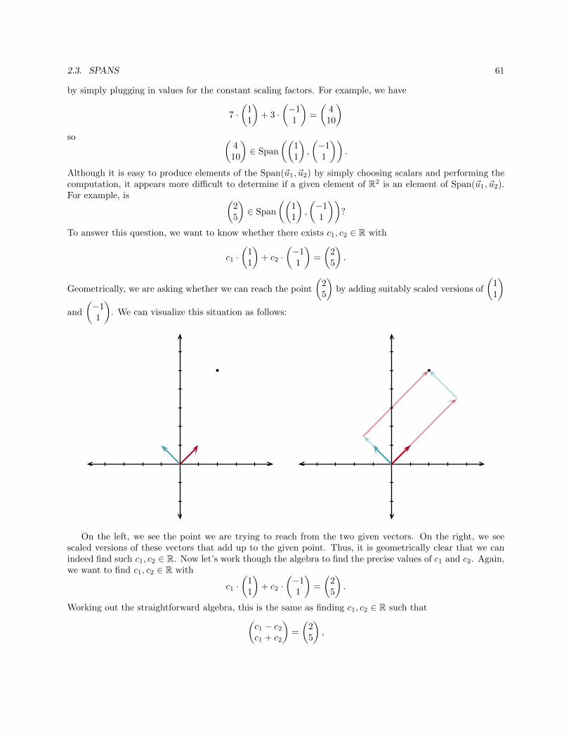
2.3. SPANS 61
by simply plugging in values for the constant scaling factors. For example, we have
7 ·(
11
)+ 3 ·
(−11
)=
(410
)so (
410
)∈ Span
((11
),
(−11
)).
Although it is easy to produce elements of the Span(~u1, ~u2) by simply choosing scalars and performing thecomputation, it appears more difficult to determine if a given element of R2 is an element of Span(~u1, ~u2).For example, is (
25
)∈ Span
((11
),
(−11
))?
To answer this question, we want to know whether there exists c1, c2 ∈ R with
c1 ·(
11
)+ c2 ·
(−11
)=
(25
).
Geometrically, we are asking whether we can reach the point
(25
)by adding suitably scaled versions of
(11
)and
(−11
). We can visualize this situation as follows:
On the left, we see the point we are trying to reach from the two given vectors. On the right, we seescaled versions of these vectors that add up to the given point. Thus, it is geometrically clear that we canindeed find such c1, c2 ∈ R. Now let’s work though the algebra to find the precise values of c1 and c2. Again,we want to find c1, c2 ∈ R with
c1 ·(
11
)+ c2 ·
(−11
)=
(25
).
Working out the straightforward algebra, this is the same as finding c1, c2 ∈ R such that(c1 − c2c1 + c2
)=
(25
),
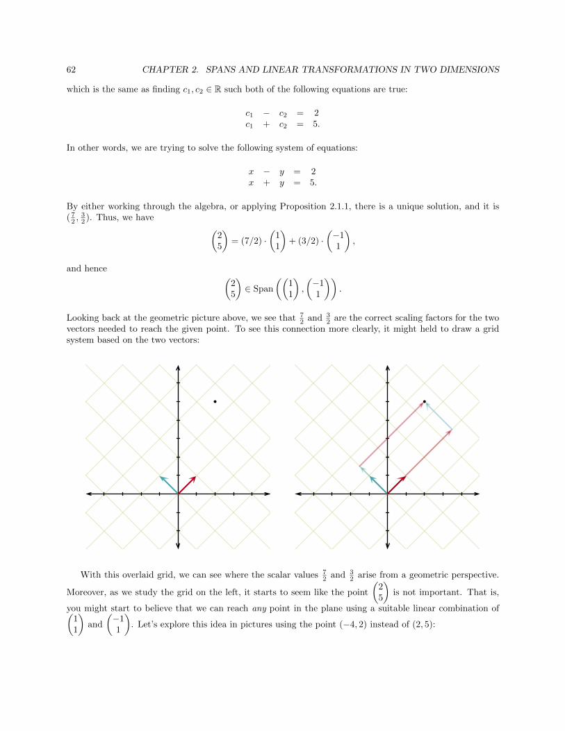
62 CHAPTER 2. SPANS AND LINEAR TRANSFORMATIONS IN TWO DIMENSIONS
which is the same as finding c1, c2 ∈ R such both of the following equations are true:
c1 − c2 = 2c1 + c2 = 5.
In other words, we are trying to solve the following system of equations:
x − y = 2x + y = 5.
By either working through the algebra, or applying Proposition 2.1.1, there is a unique solution, and it is( 72 ,
32 ). Thus, we have (
25
)= (7/2) ·
(11
)+ (3/2) ·
(−11
),
and hence (25
)∈ Span
((11
),
(−11
)).
Looking back at the geometric picture above, we see that 72 and 3
2 are the correct scaling factors for the twovectors needed to reach the given point. To see this connection more clearly, it might held to draw a gridsystem based on the two vectors:
With this overlaid grid, we can see where the scalar values 72 and 3
2 arise from a geometric perspective.
Moreover, as we study the grid on the left, it starts to seem like the point
(25
)is not important. That is,
you might start to believe that we can reach any point in the plane using a suitable linear combination of(11
)and
(−11
). Let’s explore this idea in pictures using the point (−4, 2) instead of (2, 5):
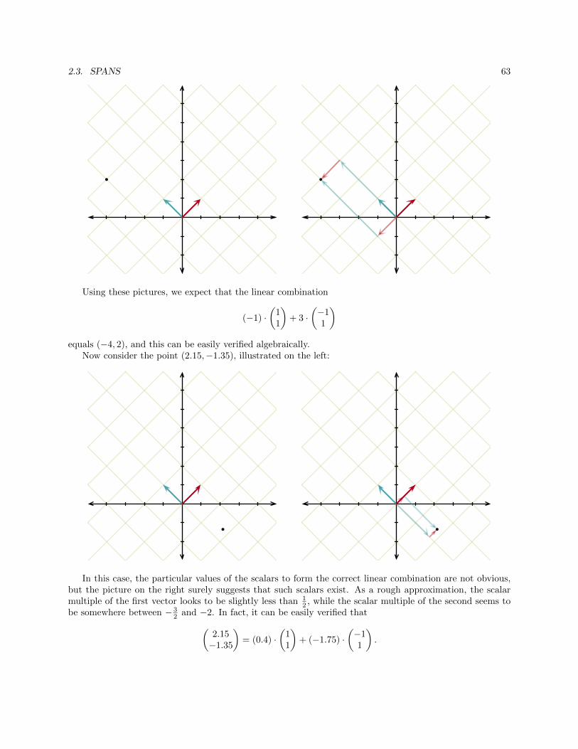
2.3. SPANS 63
Using these pictures, we expect that the linear combination
(−1) ·(
11
)+ 3 ·
(−11
)equals (−4, 2), and this can be easily verified algebraically.
Now consider the point (2.15,−1.35), illustrated on the left:
In this case, the particular values of the scalars to form the correct linear combination are not obvious,but the picture on the right surely suggests that such scalars exist. As a rough approximation, the scalarmultiple of the first vector looks to be slightly less than 1
2 , while the scalar multiple of the second seems tobe somewhere between − 3
2 and −2. In fact, it can be easily verified that(2.15−1.35
)= (0.4) ·
(11
)+ (−1.75) ·
(−11
).
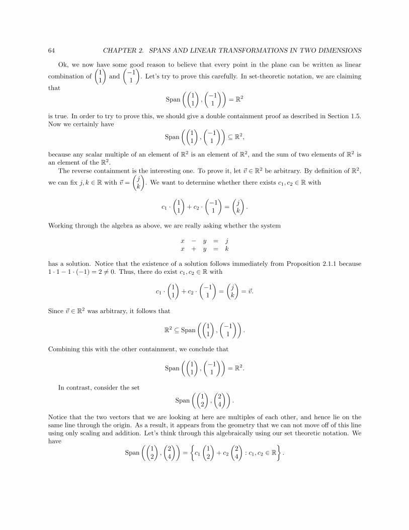
64 CHAPTER 2. SPANS AND LINEAR TRANSFORMATIONS IN TWO DIMENSIONS
Ok, we now have some good reason to believe that every point in the plane can be written as linear
combination of
(11
)and
(−11
). Let’s try to prove this carefully. In set-theoretic notation, we are claiming
that
Span
((11
),
(−11
))= R2
is true. In order to try to prove this, we should give a double containment proof as described in Section 1.5.Now we certainly have
Span
((11
),
(−11
))⊆ R2,
because any scalar multiple of an element of R2 is an element of R2, and the sum of two elements of R2 isan element of the R2.
The reverse containment is the interesting one. To prove it, let ~v ∈ R2 be arbitrary. By definition of R2,
we can fix j, k ∈ R with ~v =
(jk
). We want to determine whether there exists c1, c2 ∈ R with
c1 ·(
11
)+ c2 ·
(−11
)=
(jk
).
Working through the algebra as above, we are really asking whether the system
x − y = jx + y = k
has a solution. Notice that the existence of a solution follows immediately from Proposition 2.1.1 because1 · 1− 1 · (−1) = 2 6= 0. Thus, there do exist c1, c2 ∈ R with
c1 ·(
11
)+ c2 ·
(−11
)=
(jk
)= ~v.
Since ~v ∈ R2 was arbitrary, it follows that
R2 ⊆ Span
((11
),
(−11
)).
Combining this with the other containment, we conclude that
Span
((11
),
(−11
))= R2.
In contrast, consider the set
Span
((12
),
(24
)).
Notice that the two vectors that we are looking at here are multiples of each other, and hence lie on thesame line through the origin. As a result, it appears from the geometry that we can not move off of this lineusing only scaling and addition. Let’s think through this algebraically using our set theoretic notation. Wehave
Span
((12
),
(24
))=
{c1
(12
)+ c2
(24
): c1, c2 ∈ R
}.
2.3. SPANS 65
Now for any c1, c2 ∈ R, we have
c1
(12
)+ c2
(24
)=
(c1 + 2c22c1 + 4c2
)=
(c1 + 2c2
2 · (c1 + 2c2)
)= (c1 + 2c2)
(12
),
so since c1 + 2c2 ∈ R, we conclude that
c1
(12
)+ c2
(24
)∈ Span
((12
)).
Since this was true for any c1, c2 ∈ R, it follows that
Span
((12
),
(24
))⊆ Span
((12
)).
Now we also have
Span
((12
))⊆ Span
((12
),
(24
))(think about why), so we can conclude that
Span
((12
),
(24
))= Span
((12
)).
The next two propositions generalize these ideas.
Proposition 2.3.7. For all ~u1, ~u2 ∈ R2, we have
Span(~u1) ⊆ Span(~u1, ~u2).
Proof. Let ~u1, ~u2 ∈ R2 be arbitrary. Consider an arbitrary ~v ∈ Span(~u1). By definition, we can fix c ∈ Rwith ~v = c~u1. We then have
~v = c~u1
= c~u1 +~0
= c~u1 + 0~u2.
Since c ∈ R and 0 ∈ R, we can conclude that ~v ∈ Span(~u1, ~u2). As ~v ∈ Span(~u1) was arbitrary, it followsthat Span(~u1) ⊆ Span(~u1, ~u2).
Proposition 2.3.8. Let ~u1, ~u2 ∈ R2. The following are equivalent, i.e. if one is true, then so is the other(and hence if one is false, then so is the other).
1. Span(~u1, ~u2) = Span(~u1).
2. ~u2 ∈ Span(~u1).
Proof. Exercise.
We also have the following simple (but useful) fact because vector addition is commutative. See if youcan write up a careful proof.
66 CHAPTER 2. SPANS AND LINEAR TRANSFORMATIONS IN TWO DIMENSIONS
Proposition 2.3.9. For all ~u1, ~u2 ∈ R2, we have Span(~u1, ~u2) = Span(~u2, ~u1).
Proof. Exercise.
With all of this work in hand, we now characterize the pairs of vectors whose span is all of R2 in severaldifferent ways.
Theorem 2.3.10. Let ~u1, ~u2 ∈ R2, say
~u1 =
(ac
)and ~u2 =
(bd
).
The following are equivalent, i.e. if any one of the statements is true, then so are all of the others (and henceif any one of the statements is false, then so are all of the others).
1. For all ~v ∈ R2, there exist r1, r2 ∈ R with ~v = r1~u1 + r2~u2, i.e. Span(~u1, ~u2) = R2.
2. Both ~u1 and ~u2 are nonzero, and there does not exist r ∈ R with ~u2 = r~u1.
3. Both ~u1 and ~u2 are nonzero, and there does not exist r ∈ R with ~u1 = r~u2.
4. ad− bc 6= 0.
5. For all ~v ∈ R2, there exist a unique pair of numbers r1, r2 ∈ R with ~v = r1~u1 + r2~u2.
Proof. In order to prove that all five of these statements are equivalent, we go around in a circle. In otherwords, we prove that (1) implies (2) (i.e. if (1) is true, then (2) is true), then prove that (2) implies (3), then(3) implies (4), then (4) implies (5), and finally that (5) implies (1).
• (1) implies (2): We instead prove the contrapositive that Not(2) implies Not(1). Suppose then thatNot(2) is true, i.e. that (2) is false. We then have three possibilities:
– Case 1: Suppose that ~u1 = ~0. In this case, we have
Span(~u1, ~u2) = Span(~0, ~u2) = Span(~u2,~0)
by Proposition 2.3.9. Now ~0 ∈ Span(~u2) by Proposition 2.3.2, so
Span(~u2,~0) = Span(~u2)
by Proposition 2.3.8. Thus, we have
Span(~u1, ~u2) = Span(~u2).
Since Span(~u2) 6= R2 by Proposition 2.3.3, we conclude that Span(~u1, ~u2) 6= R2.
– Case 2: Suppose that ~u2 = ~0. In this case, we have
Span(~u1, ~u2) = Span(~u1,~0).
Now ~0 ∈ Span(~u2) by Proposition 2.3.2, so
Span(~u1,~0) = Span(~u1)
by Proposition 2.3.8. Thus, we have
Span(~u1, ~u2) = Span(~u1).
Since Span(~u1) 6= R2 by Proposition 2.3.3, we conclude that Span(~u1, ~u2) 6= R2.
2.3. SPANS 67
– Case 3: Suppose that there exists r ∈ R with ~u2 = r~u1. We then have that ~u2 ∈ Span(~u1), so
Span(~u1, ~u2) = Span(~u1)
by Proposition 2.3.8. Since Span(~u1) 6= R2 by Proposition 2.3.3, we conclude that Span(~u1, ~u2) 6=R2.
Since these cases exhaust all possibilities, it follows that Span(~u1, ~u2) 6= R2 unconditionally. Thus, (1)is false, and hence Not(1) is true.
• (2) implies (3): We instead prove the contrapositive that Not(3) implies Not(2). Suppose then thatNot(3) is true, i.e. that (3) is false. Now if either ~u1 or ~u2 is zero, then we have that Not(2) is trueand we are done. Suppose then that both ~u1 and ~u2 are nonzero. Since we are assuming that (3) isfalse, we can then fix r ∈ R with ~u1 = r~u2. Since ~u1 6= ~0, it must be the case that r 6= 0. Thus, we canmultiply both sides by 1
r to conclude that ~u2 = 1r · ~u1. Therefore, (2) is false, so Not(2) is true.
• (3) implies (4): We instead prove the contrapositive that Not(4) implies Not(3). Suppose then thatNot(4) is true, so then ad − bc = 0. Now if either ~u1 or ~u2 equals zero, then Not(3) is true and weare done. Assume then that both ~u1 and ~u2 are nonzero. We now have two cases:
– Case 1: Suppose that b = 0. Notice that we must have d 6= 0 because ~u2 is nonzero. Now sincead− bc = 0, we conclude that ad = 0, and dividing both sides by the nonzero d, we conclude thata = 0. Now notice that
c
d· ~u2 =
c
d·(bd
)=c
d·(
0d
)=
(0c
)=
(ac
)= ~u1.
Since cd ∈ R, we have verified that Not(3) is true.
– Case 2: Suppose that b 6= 0. Since ad− bc = 0, we must have that ad = bc. Now b 6= 0, so we candivide both sides by it to conclude that ad
b = c. Now notice that
a
b· ~u2 =
a
b·(bd
)=
(aadb
)=
(ac
)(from above)
= ~u1.
Since ab ∈ R, we have verified that Not(3) is true by showing that there does exist r ∈ R with
~u1 = r~u2.
Since the two cases exhaust all possibilities, we conclude that Not(3) is true unconditionally, whichcompletes the proof.
68 CHAPTER 2. SPANS AND LINEAR TRANSFORMATIONS IN TWO DIMENSIONS
• (4) implies (5): Suppose that (4) is true, so we are assuming that ad− bc 6= 0. Let ~v ∈ R2 be arbitrary,and fix j, k ∈ R with ~v = (j, k). Since ad − bc 6= 0, we can use Proposition 2.1.1 to conclude that thesystem
ax + by = jcx + dy = k
has a unique solution. From this, it follows that there is a unique solution to
x
(ac
)+ y
(bd
)=
(jk
),
which is the same as saying that there exists a unique pair of numbers r1, r2 ∈ R with ~v = r1~u1 + r2~u2.Since ~v ∈ R2 was arbitrary, we conclude that (5) is true.
• (5) implies (1): This is immediate because (5) is just a strengthening of (1) (if there exists a uniquepair of numbers, then there certainly exists a pair of numbers).
Suppose then that we have ~u1, ~u2 ∈ R2 with Span(~u1, ~u2) = R2. By definition, we can express every~v ∈ R2 as a linear combination of ~u1 and ~u2. However, by the theorem we just proved, we now know thestronger fact that no matter which ~v ∈ R2 we have, we can always find unique scaling factors c1 and c2 in Rto apply to ~u1 and ~u2 so that the corresponding linear combination equals ~v. Since this stronger propertyof uniqueness is fundamental, we introduce new, more concise, terminology to describe this situation.
Definition 2.3.11. Let ~u1, ~u2 ∈ R2. We say that the ordered pair (~u1, ~u2) is a basis for R2 if Span(~u1, ~u2) =R2.
We will often use lowercase Greek letters, like α or β, to denote a basis. For example, suppose that
~u1 =
(51
)and ~u2 =
(−6−3
).
Notice that 5 · (−3)− 1 · (−6) = −9, so Span(~u1, ~u2) = R2 by Theorem 2.3.10. If we let α denote the orderedpair (~u1, ~u2), i.e. let
α =
((51
),
(−6−3
)),
then α is a basis of R2.As we will see, bases will play an essential role throughout our study. What makes them so special?
Intuitively, our two fundamental operations on vectors are addition and scalar multiplication. If we have abasis α, then we can reach all elements of R2 from the vectors in α by using only these two operations. Thus,if we have a function f : R2 → R2, and we know (for some reason) how f interacts with addition and scalarmultiplication, then we can use knowledge of how f behaves on a basis α to understand how f behaves onother inputs. With this idea in mind, we turn now to special functions that behave well with respect toaddition and scalar multiplication.
2.4 Linear Transformations of R2
Back in Section 1.1, we discussed a function T : R2 → R2 defined by letting
T
((xy
))=
(x− yx+ y
).
Computing the values on some of the points, we obtain the following:
2.4. LINEAR TRANSFORMATIONS OF R2 69
• T((
10
))=
(11
).
• T((
01
))=
(−11
).
• T((
11
))=
(02
).
As mentioned in Section 1.1, by computing the values at enough points, it starts to look like T might berotating the plane by 45o counterclockwise around the origin, and also scaling the plane by a factor of
√2.
Before delving into this idea further, let’s take a step back and think about a somewhat philosophicalquestion. In this example, we computed a few points and used those to make a guess about what wouldhappen on other points. Is it reasonable to believe that we can make global predictions based on a few points?Given a function f : R→ R, if we know the values of f at several points, can we use those values to predictwhat f will be at other points? Without some sort of additional assumption, it seems impossible to predictthe values of f on other points, because f could be piecewise-defined or worse. Now in the natural sciencesand in statistics, you often extrapolate from certain data points to a general function that fits the pointswell, at least up to small errors. The general philosophical assumptions underlying such an extrapolationis that the function that we are searching for is not random or erratic, but somehow will be constrained tobehave in reasonable ways. In these areas, we tend to follow this approach either because we believe in thefundamentally regularity and simplicity of nature, or because we need to make some simplifying assumptionsto make any sort of reasonable predictions.
However, in mathematics, we want to be precise and codify what we mean by saying something like“the function f is not random or erratic” or “the function f has nice structural properties” so that we canunderstand the assumptions behind these models. We could make the assumption that “f is a polynomial”,which will restrict the possibilities. In calculus, you might make the assumption that “f is continuous” toavoid large jumps in the function, or even assume the more restrictive assumption that “f is differentiableeverywhere and −3 ≤ f ′(x) ≤ 3 for all x ∈ R” so that the function will be smooth and neither increase nordecrease too rapidly.
Returning to our function T above, it turns out that it has a couple of really interesting structuralproperties that restrict its behavior. Let ~v1, ~v2 ∈ R2 be arbitrary, and fix x1, y1, x2, y2 ∈ R with
~v1 =
(x1y1
)and ~v2 =
(x2y2
).
Notice that
T (~v1 + ~v2) = T
((x1y1
)+
(x2y2
))= T
((x1 + x2y1 + y2
))=
(x1 + x2 − (y1 + y2)x1 + x2 + y1 + y2
)=
(x1 − y1 + x2 − y2x1 + x2 + y1 + y2
)=
(x1 − y1x1 + y1
)+
(x2 − y2x2 + y2
)= T
((x1y1
))+ T
((x2y2
))= T (~v1) + T (~v2).
70 CHAPTER 2. SPANS AND LINEAR TRANSFORMATIONS IN TWO DIMENSIONS
In other words, we can interchange the order between adding vectors and applying T . That is, we can eitheradd two vectors first, and then apply the function T , or we can apply the function T to each vector, andthen add the results. This is a remarkable property! Very (very) few functions f : R→ R have the propertythat f(a + b) = f(a) + f(b) for all a, b ∈ R. For example, in general, (a + b)2 does not equal a2 + b2, andsin(a+ b) does not equal sin a+ sin b.
However, if we think geometrically about a rotation around the origin by a fixed angle θ, it appears thatsuch a rotation also has this property. Given two vectors ~v1 and ~v2 in R2, it looks like the following twooperations result in the same vector:
• First add the vectors to form ~v1 + ~v2, and then rotate the result by θ.
• First rotate ~v1 and ~v2 each by θ, and then add the results.
Beyond addition, the other fundamental operation on vectors is scalar multiplication. Let ~v ∈ R2 andc ∈ R be arbitrary, and fix x, y ∈ R with
~v =
(xy
).
Notice that
T (c · ~v) = T
(c ·(xy
))= T
((cxcy
))=
(cx− cycx+ cy
)=
(c · (x− y)c · (x+ y)
)= c ·
(x− yx+ y
)= c · T
((xy
))= c · T (~v).
Thus, we can interchange the order between scalar multiplication and applying T . Just like for addition,rotation behaves well with respect to scalar multiplication. More precisely, given a vector ~v ∈ R2 and anumber c ∈ R, it looks like the following two operations results in the same vector:
• First scale ~v by c to form c · ~v, and then rotate the result by θ.
• First rotate ~v by θ, and then scale the result by c.
Functions from R2 to R2 that respect the two basic operations of vector addition and scalar multiplicationare given a special name, and will be a fundamental object of our study.
Definition 2.4.1. A linear transformation from R2 to R2 is a function T : R2 → R2 with the following twoproperties:
1. T (~v1 + ~v2) = T (~v1) + T (~v2) for all ~v1, ~v2 ∈ R2 (i.e. T preserves addition).
2. T (c · ~v) = c · T (~v) for all ~v ∈ R2 and c ∈ R (i.e. T preserves scalar multiplication).
2.4. LINEAR TRANSFORMATIONS OF R2 71
Consider the function T : R2 → R2 defined by
T
((xy
))=
(x2 + y
5x
).
Is T a linear transformation? If we try to compute whether T preserves addition, we might notice that
T
((x1y1
)+
(x2y2
))= T
((x1 + x2y1 + y2
))=
((x1 + x2)2 + (y1 + y2)
5 · (x1 + x2)
)=
(x21 + 2x1x2 + x22 + y1 + y2
5x1 + 5x2
),
while
T
((x1y1
))+ T
((x2y2
))=
(x21 + y1
5x1
)+
(x22 + y2
5x2
)=
(x21 + x22 + y1 + y2
5x1 + 5x2
).
Since one of these has an extra 2x1x2 in the first coordinate, it appears that these two outputs are not thesame. However, looks can be deceiving, and occasionally different looking formulas can produce the sameoutput on all inputs (like the fact that sin(2x) equals 2 sinx cosx for all x ∈ R). In order to argue thatT is not a linear transformation, we should instead give a specific counterexample. Looking at the abovecomputation, we should probably choose two vectors whose first coordinate is nonzero. Notice that
T
((10
)+
(20
))= T
((30
))=
(32 + 0
5 · (3 + 0)
)=
(915
),
while
T
((10
))+ T
((20
))=
(12 + 05 · 1
)+
(22 + 05 · 2
)=
(15
)+
(410
)=
(515
).
Therefore, we have
T
((10
)+
(20
))6= T
((10
))+ T
((20
)),
so T is not a linear transformation.In contrast, let’s take a look at the function T : R2 → R2 given by
T
((xy
))=
(x+ 3yy
).
72 CHAPTER 2. SPANS AND LINEAR TRANSFORMATIONS IN TWO DIMENSIONS
It turns out that T is a linear transformation (this fact will follow from Proposition 2.4.3 below, but it’sworth working through the argument carefully on your own). Let’s examine how this linear transformationbehaves. Trying out a few points on the x-axis, we see that
T
((10
))=
(10
)and T
((20
))=
(20
)In fact, for any x ∈ R, we have
T
((x0
))=
(x+ 3 · 0
0
)=
(x0
),
so every point on the x-axis is fixed. Looking at the line y = 1, we see for that x ∈ R, we have
T
((x1
))=
(x+ 3 · 1
1
)=
(x+ 3
1
),
so the line y = 1 is shifted to the right by 3. A similar computation shows that the line y = 2 is shiftedto the right by 6, the line y = 1
3 is shifted to the right by 1, and the line y = −1 is shifted to the left by3. Examining the formula again, it becomes clear geometrically that for a fixed c, the line y = c is shiftedto the right by 3c when c is positive, and is shifted to the left by 3c when c is negative. Thus, T takes theplane and “shifts” it along horizontal lines, with the shift becoming larger as we move away from the x-axis.A linear transformation T of this type is called a shear transformation.
Proposition 2.4.2. Let T : R2 → R2 be a linear transformation. We have the following:
1. T (~0) = ~0.
2. T (−~v) = −T (~v) for all ~v ∈ R2.
3. T (c1~v1 + c2~v2) = c1 · T (~v1) + c2 · T (~v2) for all ~v1, ~v2 ∈ R2 and all c1, c2 ∈ R.
Proof.
1. Notice that
T (~0) = T (~0 +~0)
= T (~0) + T (~0) (since T preserves addition),
so T (~0) = T (~0) + T (~0). Subtracting the vector T (~0) from both sides, we conclude that
~0 = T (~0),
which completes the proof of 1.
2. Let ~v ∈ R2 be arbitrary. Notice that
T (−~v) = T ((−1) · ~v)
= (−1) · T (~v) (since T preserves scalar multiplication)
= −T (~v).
Since ~v ∈ R2 was arbitrary, this completes the proof of 2.
2.4. LINEAR TRANSFORMATIONS OF R2 73
3. Let ~v1, ~v2 ∈ R2 and c1, c2 ∈ R be arbitrary. Since c1~v1 and c2~v2 are both elements of R2, we have
T (c1~v1 + c2~v2) = T (c1~v1) + T (c2~v2) (since T preserves addition)
= c1 · T (~v1) + c2 · T (~v2) (since T preserves scalar multiplication).
Since ~v1, ~v2 ∈ R2 and c1, c2 ∈ R were arbitrary, this completes the proof of 3.
Let’s return to our above example of a linear transformation T : R2 → R2 given by
T
((xy
))=
(x− yx+ y
).
Notice that we can also write T as
T
((xy
))=
(xx
)+
(−yy
)= x ·
(11
)+ y ·
(−11
).
In other words, we can view T as follows. For any x, y ∈ R:
T sends
(xy
)to the linear combination of
(11
)and
(−11
)given by using the scalars x and y.
Hence, in this case, we see that our linear transformation T can be viewed through the lens of linearcombinations. Moreover, T sends (x, y) to the point obtained by making a grid system using the vectors(1, 1) and (−1, 1), and then finding the point that is x units along (1, 1) and y units along (−1, 1).
Similarly, if we look at the linear transformation T : R2 → R2 given by
T
((xy
))=
(x+ 3yy
),
then we can also write T as
T
((xy
))= x ·
(10
)+ y ·
(31
).
Thus, we can view T has taking a vector (x, y) and using its values as coordinates within the grid systemformed by (1, 0) and (3, 1).
Proposition 2.4.3. Let a, b, c, d ∈ R. Define a function T : R2 → R2 by
T
((xy
))=
(ax+ bycx+ dy
)= x ·
(ac
)+ y ·
(bd
).
We then have that T is a linear transformation.
Proof. To prove that T is a linear transformation, we need to check that T preserves both addition andscalar multiplication.
74 CHAPTER 2. SPANS AND LINEAR TRANSFORMATIONS IN TWO DIMENSIONS
• We first check that T preserves addition. Let ~v1, ~v2 ∈ R2 be arbitrary. Fix x1, y1, x2, y2 ∈ R with
~v1 =
(x1y1
)and ~v2 =
(x2y2
).
We have
T (~v1 + ~v2) = T
((x1y1
)+
(x2y2
))= T
((x1 + x2y1 + y2
))=
(a(x1 + x2) + b(y1 + y2)c(x1 + x2) + d(y1 + y2)
)=
(ax1 + ax2 + by1 + by2cx1 + cx2 + dy1 + dy2
)=
(ax1 + by1 + ax2 + by2cx1 + dy1 + cx2 + dy2
)=
(ax1 + by1cx1 + dy1
)+
(ax2 + by2cx2 + dy2
)= T
((x1y1
))+ T
((x2y2
))= T (~v1) + T (~v2).
Since ~v1, ~v2 ∈ R2 were arbitrary, it follows that T preserves addition.
• We now check that T preserves scalar multiplication. Let ~v ∈ R2 and r ∈ R be arbitrary. Fix x, y ∈ Rwith
~v =
(xy
).
We have
T (r · ~v) = T
(r ·(xy
))= T
((rxry
))=
(a(rx) + b(ry)c(rx) + c(ry)
)=
(rax+ rbyrcx+ rcy
)= r ·
(ax+ bycx+ dy
)= r · T
((xy
))= r · T (~v).
Since ~v ∈ R2 and r ∈ R were arbitrary, it follows that T preserves scalar multiplication.
We’ve shown that T preserves both addition and scalar multiplication, so T is a linear transformation.
2.4. LINEAR TRANSFORMATIONS OF R2 75
With this result in hand, we now have an infinite stock of examples of linear transformations from R2 toR2.
Suppose that we have a function T : R2 → R2, and assume that we know that T is a linear transformationwith both
T
((10
))=
(32
)and T
((01
))=
(−17
).
Can we compute other values of T? It turns out that this is possible for all other inputs of T . For example,to determine
T
((83
))we can first notice that (
83
)= 8 ·
(10
)+ 3 ·
(01
),
so we have
T
((83
))= T
(8 ·(
10
)+ 3 ·
(01
))= 8 · T
((10
))+ 3 · T
((01
))(by Proposition 2.4.2)
= 8 ·(
32
)+ 3 ·
(−17
)=
(2137
).
There was nothing special about the vector
(83
)here. Using the same technique, we can determine the
value of T
((ab
))for any a, b ∈ R by simply noticing that
(ab
)= a ·
(10
)+ b ·
(01
)and using the fact that T is a linear transformation.
In the previous example, we assumed that we knew the values of T on the two basic vectors (1, 0) and(0, 1). Suppose instead that we know that values of T on different inputs. For example, suppose thatT : R2 → R2 is a linear transformation, and that we know that
T
((28
))=
(32
)and T
((1−3
))=
(−17
).
Can we compute other values of T? Although the process is slightly more involved, we can indeed determinethe value of T on all other inputs. The key fact here is that
Span
((28
),
(1−3
))= R2
because 2 · (−3)− 8 · 1 = −14, which is nonzero. Thus, given any vector ~v ∈ R2, we can express ~v as a linearcombination of (
28
)and
(1−3
),
76 CHAPTER 2. SPANS AND LINEAR TRANSFORMATIONS IN TWO DIMENSIONS
and then use the fact that T is a linear transformation to determine T (~v). For example, if we want todetermine
T
((91
)),
we first find the unique pair of numbers c1, c2 ∈ R with(91
)= c1 ·
(28
)+ c2 ·
(1−3
).
Working through the algebra, it turns out that(91
)= 2 ·
(28
)+ 5 ·
(1−3
).
From this, we conclude that
T
((91
))= T
(2 ·(
28
)+ 5 ·
(1−3
))= 2 · T
((28
))+ 5 · T
((1−3
))(by Proposition 2.4.2)
= 2 ·(
32
)+ 5 ·
(−17
)=
(139
).
Generalizing these ideas leads to the conclusion that if T : R2 → R2 is a linear transformation and ~u1, ~u2 ∈ R2
satisfy Span(~u1, ~u2) = R2, then T is completely determined by the two values T (~u1) and T (~u2). We statethis “completely determined” property formally in the following way.
Theorem 2.4.4. Let α = (~u1, ~u2) be a basis of R2. Suppose that T : R2 → R2 and S : R2 → R2 are lineartransformations with the property that T (~u1) = S(~u1) and T (~u2) = S(~u2). We then have that T = S,i.e. T (~v) = S(~v) for all ~v ∈ R2.
Proof. Let ~v ∈ R2 be arbitrary. Since α is a basis of R2, we can fix c1, c2 ∈ R with
~v = c1~u1 + c2~u2.
We then have
T (~v) = T (c1~u1 + c2~u2)
= c1 · T (~u1) + c2 · T (~u2) (by Proposition 2.4.2)
= c1 · S(~u1) + c2 · S(~u2) (by assumption)
= S(c1~u1 + c2~u2) (by Proposition 2.4.2)
= S(~v).
Since ~v ∈ R2 was arbitrary, it follows that T = S.
Notice that the theorem we just proved says nothing about what happens if α = (~u1, ~u2) is not a basisof R2. For example, if T : R2 → R2 is a linear transformation and we know that
T
((10
))=
(41
)and T
((20
))=
(82
),
2.4. LINEAR TRANSFORMATIONS OF R2 77
then it seems impossible to determine
T
((01
))because (
01
)/∈ Span
((10
),
(20
)).
Up until now, we have determined other values of T under the assumption that we had a linear transfor-mation T that produced certain outputs on a couple of given values. We have not yet dealt with the questionof whether such a linear transformation T exists at all. In other words, we’ve discussed a uniqueness question(there is at most one such linear transformation) without addressing the corresponding existence question(whether there is at least one). For instance, if we change the values above and think about whether thereis a linear transformation T : R2 → R with
T
((10
))=
(41
)and T
((20
))=
(53
),
then we can quickly see that no such T exists. Why? If T : R2 → R2 is a linear transformation with
T
((10
))=
(41
),
then we must have
T
((20
))= T
(2 ·(
10
))= 2 · T
((10
))= 2 ·
(41
)=
(82
).
In this instance, we run into a problem because our two vectors are multiples of each other. What happensif this is not the case?
Returning to our example before the proposition, we may ask whether there exists a linear transformationT : R2 → R2 such that
T
((10
))=
(32
)and T
((01
))=
(−17
).
Now in this situation, there is no clear conflict like the one above, but it is also not obvious whether sucha linear transformation exists. To prove the existence of such a T , it looks like we need to build it directly.Clearly, there is a function f : R2 → R2 with
f
((10
))=
(32
)and f
((01
))=
(−17
)because we can just define f like this on these two points and define it to be ~0 everywhere else. However,such a piecewise defined function is unlikely to be a linear transformation (and the given f certainly isnot). In order to try to obtain a linear transformation T with these properties, we can look to Proposition
78 CHAPTER 2. SPANS AND LINEAR TRANSFORMATIONS IN TWO DIMENSIONS
2.4.3, which provides an infinite supply of linear transformations. From this perspective, we want to choosea, b, c, d ∈ R so that if we let
T
((xy
))=
(ax+ bycx+ dy
),
then we will have
T
((10
))=
(32
)and T
((01
))=
(−17
).
Working through the simple algebra, we see that it works if we let a = 3, b = −1, c = 2, and d = 7. In otherwords, the function T : R2 → R2 defined by
T
((xy
))=
(3x− y2x+ 7y
)is a linear transformation (by Proposition 2.4.3) that takes the correct values on our two points. There wasnothing special about the vectors (3, 2) and (−1, 7). In fact, for any choice of a, b, c, d ∈ R, there exists alinear transformation T : R2 → R2 such that
T
((10
))=
(ac
)and T
((01
))=
(bd
),
namely
T
((xy
))=
(ax+ bycx+ dy
).
However, this simple construction does not work as easily if we change the input vectors away from (1, 0)and (0, 1).
Returning to the other example above, we may ask whether there exists a linear transformation T : R2 →R2 such that
T
((28
))=
(32
)and T
((1−3
))=
(−17
).
In this case, it’s much harder to try to directly build a, b, c, d ∈ R to make this happen. Although it is certainlypossible to work through the algebra directly, we instead take a different approach here (we will eventuallysee a more direct computational approach that avoids the ugly algebra just alluded to). Rather than buildT through a formula, we instead build T more abstractly. Before diving into the general description of T ,let’s consider how T would have to behave on some specific inputs. For example, we must have
T
((3−9
))= T
(3 ·(
1−3
))= 3 · T
((1−3
))= 3 ·
(−17
)=
(−321
).
2.4. LINEAR TRANSFORMATIONS OF R2 79
We would also need
T
((35
))= T
((28
)+
(1−3
))= T
((28
))+ T
((1−3
))=
(32
)+
(−17
)=
(29
).
Following in a similar manner, we can determine what T (~v) would have to be for any ~v ∈ R2 because
Span
((28
),
(1−3
))= R2.
These computations provide us with a candidate function for T . Now we turn this around by simply defininga function T : R2 → R2 in this way, and check that the resulting function is in fact a linear transformation.Here is the general argument.
Theorem 2.4.5. Let α = (~u1, ~u2) be a basis of R2, and let ~w1, ~w2 ∈ R2. There exists a linear transformationT : R2 → R2 with T (~u1) = ~w1 and T (~u2) = ~w2.
Before jumping into the proof, notice that we are not assuming that Span(~w1, ~w2) = R2, as such anassumption is unnecessary.
Proof. Define a function T : R2 → R2 as follows. Given ~v ∈ R2, fix the unique pair c1, c2 ∈ R with~v = c1~u1 + c2~u2, and define
T (~v) = c1 ~w1 + c2 ~w2.
Notice that we have described T completely as a function, so we need only check that it is a linear transfor-mation with the required properties.
• We first check that T preserves addition. Let ~v1, ~v2 ∈ R2 be arbitrary. Since Span(~u1, ~u2) = R2 byassumption, we can apply Theorem 2.3.10 to fix the unique pair of numbers c1, c2 ∈ R with
~v1 = c1~u1 + c2~u2,
and also to fix the unique pair of numbers d1, d2 ∈ R2 with
~v2 = d1~u1 + d2~u2.
We then have
~v1 + ~v2 = (c1~u1 + c2~u2) + (d1~u1 + d2~u2)
= (c1 + d1)~u1 + (c2 + d2)~u2,
hence
T (~v1 + ~v2) = (c1 + d1)~w1 + (c2 + d2)~w2 (by definition of T )
= c1 ~w1 + d1 ~w1 + c2 ~w2 + d2 ~w2
= c1 ~w1 + c2 ~w2 + d1 ~w1 + d2 ~w2
= T (~v1) + T (~v2) (by definition of T ).
Since ~v1, ~v2 ∈ R2 were arbitrary, it follows that T preserves addition.
80 CHAPTER 2. SPANS AND LINEAR TRANSFORMATIONS IN TWO DIMENSIONS
• We next check that T preserves scalar multiplication. Let ~v ∈ R2 and c ∈ R be arbitrary. SinceSpan(~u1, ~u2) = R2 by assumption, we can apply Theorem 2.3.10 and fix the unique pair of numbersd1, d2 ∈ R with
~v = d1~u1 + d2~u2.
We then have
c · ~v = c · (d1~u1 + d2~u2)
= (cd1)~u1 + (cd2)~u2,
hence
T (c · ~v) = (cd1)~w1 + (cd2)~w2 (by definition of T )
= c · (d1 ~w1 + d2 ~w2)
= c · T (~v) (by definition of T ).
Since ~v ∈ R2 and c ∈ R were arbitrary, it follows that T preserves scalar multiplication.
• We finally check that T (~u1) = ~w1 and T (~u2) = ~w2. Notice that
~u1 = 1 · ~u1 + 0 · ~u2
so by definition of T , we have
T (~u1) = 1 · ~w1 + 0 · ~w2
= ~w1.
Similarly, we have
~u2 = 0 · ~u1 + 1 · ~u2
so by definition of T , we have
T (~u2) = 0 · ~w1 + 1 · ~w2
= ~w2.
To recap, we have built a function T : R2 → R2 that is a linear transformation and satisfies both T (~u1) = ~w1
and T (~u2) = ~w2. This completes the proof.
As we’ve mentioned, linear transformations are the functions from R2 to R2 that are “nice” from thepoint of view of linear algebra. In Calculus, you think of a function f : R → R as being “nice” if it isdifferentiable (or maybe continuous). Now back in Calculus, you talk about results that say that if youcombine two “nice” functions in a basic way, then the resulting function is “nice” as well. For example, wehave the following.
• If f : R→ R and g : R→ R are both differentiable functions, then the function f + g : R→ R definedby (f + g)(x) = f(x) + g(x) for all x ∈ R is also a differentiable function. Moreover, you learn how tocompute (f + g)′ in terms of the f ′ and g′. This is the Sum Rule.
• If f : R → R and g : R → R are both differentiable functions, then the function f · g : R → R definedby (f · g)(x) = f(x) · g(x) for all x ∈ R is also a differentiable function. Moreover, you learn how tocompute (f · g)′ in terms of the f ′ and g′. This is the Product Rule.
2.4. LINEAR TRANSFORMATIONS OF R2 81
• If f : R→ R and g : R→ R are both differentiable functions, then the function f ◦g : R→ R defined by(f ◦ g)(x) = f(g(x)) for all x ∈ R is also a differentiable function. Moreover, you learn how to compute(f ◦ g)′ in terms of the f ′ and g′. This is the Chain Rule.
We could also think about other ways to build new functions from old, such as taking the quotient of twofunctions (as long as the denominator is nonzero), or multiplying a function by a constant (although thiscan be seen as a special case of the Product Rule).
We want to ask similar questions about linear transformations. Suppose that T : R2 → R2 and S : R2 →R2 are both linear transformations. What operations can we perform on them? Recall that linear transfor-mations are certain special types of functions. We can certainly add the two functions T and S by addingthem pointwise like we do in Calculus, except now we are adding the output vectors rather than the outputreal numbers. Although this provides a well-defined function, it is not completely obvious that the resultingfunction is a linear transformation. It seems reasonable to believe this might be true because linear transfor-mations “play nice” with addition. We will verify that the resulting function is indeed a linear transformationin Proposition 2.4.7 below.
Can we also multiply T and S together? If we try to do it in the naive manner, then we need tounderstand how we will define the multiplication of two output vectors in R2. We could define multiplicationcomponentwise, but such a definition lacks a nice geometric interpretation, and it feels unlikely that theresulting function is a linear transformation anyway (since the span of a vector is not closed under such anoperation). We might consider the dot product, but then remember that the dot product of two elements ofR2 is an element of R rather than an element of R2. Although we can try to think of other potential ways todefine a multiplication of vectors, it seems improbable that any of these will result in a linear transformationanyway. In place of a general notion of multiplication of linear transformations, we can instead think ofmultiplying a linear transformation by a scalar, just as we do for Calculus functions (i.e. we can multiplythe function f(x) = x2 by 5 to obtain the function g(x) = 5x2). Since linear transformations “play nice”with scalar multiplication, there is a reasonable hope that the result is a linear transformation.
Definition 2.4.6. We define the following:
• Let T : R2 → R2 and S : R2 → R2 be functions. We define a new function T + S : R2 → R2 by letting(T + S)(~v) = T (~v) + S(~v) for all ~v ∈ R2.
• Let T : R2 → R2 be a functions and let r ∈ R. We define a new function r · T : R2 → R2 by letting(r · T )(~v) = r · T (~v) for all ~v ∈ R2.
Now that we have defined these operations, we argue that if T and S are both linear transformations,then their sum is also a linear transformation (and similarly for scalar multiplication). Moreover, we alsoshow that the composition of two linear transformations is a linear transformation. Recall that we definedthe composition of two functions f and g generally in Definition 1.6.4, as long as the codomain of thefunction on the right equals the domain of the function on the left. Since both of these equal R2 for lineartransformations, we can indeed also perform composition.
Proposition 2.4.7. Let T, S : R2 → R2 be linear transformations.
1. The function T + S is a linear transformation.
2. For all r ∈ R, then function r · T is a linear transformation.
3. The function T ◦ S is a linear transformation.
Proof. We prove each statement individually:
82 CHAPTER 2. SPANS AND LINEAR TRANSFORMATIONS IN TWO DIMENSIONS
1. We first check that T + S preserves addition. Let ~v1, ~v2 ∈ R2 be arbitrary. We have
(T + S)(~v1 + ~v2) = T (~v1 + ~v2) + S(~v1 + ~v2) (by definition)
= T (~v1) + T (~v2) + S(~v1) + S(~v2) (since T and S are linear transformations)
= T (~v1) + S(~v1) + T (~v2) + S(~v2)
= (T + S)(~v1) + (T + S)(~v2) (by definition).
Therefore, the function T + S preserves addition.
We now check that T +S preserves scalar multiplication. Let ~v ∈ R2 and c ∈ R be arbitrary. We have
(T + S)(c · ~v) = T (c · ~v) + S(c · ~v) (by definition)
= c · T (~v) + c · S(~v) (since T and S are linear transformations)
= c · (T (~v) + S(~v))
= c · (T + S)(~v) (by definition).
Therefore, the function T + S preserves scalar multiplication as well. It follows that T + S is a lineartransformation.
2. Let r ∈ R be arbitrary. We first check that r · T preserves addition. Let ~v1, ~v2 ∈ R2 be arbitrary. Wehave
(r · T )(~v1 + ~v2) = r · T (~v1 + ~v2) (by definition)
= r · (T (~v1) + T (~v2)) (since T is a linear transformation)
= r · T (~v1) + r · T (~v1)
= (r · T )(~v1) + (r · T )(~v2) (by definition).
Therefore, the function r · T preserves addition.
We now check that r · T preserves scalar multiplication. Let ~v ∈ R2 and c ∈ R be arbitrary. We have
(r · T )(c · ~v) = r · T (c · ~v) (by definition)
= r · (c · T (~v)) (since T is a linear transformation)
= (rc) · T (~v)
= (cr) · T (~v)
= c · (r · T (~v))
= c · (r · T )(~v) (by definition).
Therefore, the function r · T preserves scalar multiplication as well. It follows that r · T is a lineartransformation.
3. Exercise.
2.5 The Standard Matrix of a Linear Transformation
In this section, we develop some shorthand notation for referring to a linear transformation T : R2 → R2 andits action on vectors in R2 (i.e. the result of plugging ~v into T to form T (~v)). In Calculus, the notation dy
dx forderivatives aids both computation and theoretical discussions because it greatly simplifies what one needs
2.5. THE STANDARD MATRIX OF A LINEAR TRANSFORMATION 83
to think about, naturally reminds us of the limit operation that defines a derivative, and suggests derivativeand integral rules that turn out to be true. We want to develop some concise and efficient notation for linearalgebra that provide similar benefits.
Throughout this section, we will denote the two standard unit vectors along the axes with the followingnotation:
~e1 =
(10
)and ~e2 =
(01
)Notice that Span(~e1, ~e2) = R2, either by directly working with the definition of Span(~e1, ~e2), or by simplyusing Theorem 2.3.10 together with the fact that 1 · 1− 0 · 0 = 1.
Suppose now that a, b, c, d ∈ R. We know from Theorem 2.4.5 and Proposition 2.4.4 that there exists aunique linear transformation T : R2 → R2 such that
T (~e1) =
(ac
)and T (~e2) =
(bd
).
In other words, the two vectors T (~e1) and T (~e2) encode everything there is to know about T . Therefore, alinear transformation T : R2 → R2 is completely determined by 4 numbers (i.e. the 4 numbers comprisingthe two vectors T (~e1) and T (~e2)). Instead of writing down the two vectors
T (~e1) =
(ac
)and T (~e2) =
(bd
)in order, we can arrange them in a certain 2× 2 table:(
a bc d
).
We call such a table a matrix, or more specifically a 2× 2 matrix. In other words, a 2× 2 matrix is just anarrangement of 4 real numbers into 2 rows and 2 columns, where the position of a number matters (like a4-tuple). We will eventually see many uses for matrices and interpret their table structure in different waysdepending on the context. However, for the moment, we want to think of a matrix as “coding” a lineartransformation. To enable this, we will use the following terminology.
Definition 2.5.1. Let T : R2 → R2 be a linear transformation. Fix a, b, c, d ∈ R with
T (~e1) =
(ac
)and T (~e2) =
(bd
).
We define the standard matrix of T to be the following 2× 2 matrix:(a bc d
).
In other words, the standard matrix of T has the entries of T (~e1) in the first column, and the entries ofT (~e2) in the second column.
Notation 2.5.2. If T : R2 → R2 is a linear transformation, then we use the notation [T ] to denote thestandard matrix of T .
As mentioned, we want to think of the standard matrix as a shorthand “code” for the correspondinglinear transformation. That is, instead of saying:
Consider the unique linear transformation T : R2 → R2 such that T (~e1) =
(ac
)and T (~e2) =
(bd
),
84 CHAPTER 2. SPANS AND LINEAR TRANSFORMATIONS IN TWO DIMENSIONS
we can instead simply say:
Consider the linear transformation with standard matrix
(a bc d
).
Now we want to push this shorthand notation further by developing a more succinct notation for plugginga vector as input into the function T . Recall that if we know the values of T on the vectors ~e1 and ~e2, thenwe can in fact determine a formula for T on an arbitrary vector as follows. Assuming that
T (~e1) =
(ac
)and T (~e2) =
(bd
),
then for any x, y ∈ R, we have
T
((xy
))= T
(x ·(
10
)+ y ·
(01
))= T (x · ~e1 + y · ~e2)
= x · T (~e1) + y · T (~e2)
= x ·(ac
)+ y ·
(bd
)=
(ax+ bycx+ dy
).
Since we are using this matrix to “code” the linear transformation T , can we create natural notation thatdispenses with T entirely and instead just uses the standard matrix? A function T : R2 → R2 takes a vector~v ∈ R2 and feeds it in as input in order to form the output T (~v). We can replace the direct reference tothe function T by instead using the standard matrix [T ], but now rather than feeding ~v as an input to T(resulting in the notation T (~v)), we instead think of “hitting” ~v with the matrix [T ]. Thus, if
~v =
(xy
)then we will write (
a bc d
)(xy
)in place of the usual function notation T (~v). If we want to make this notation match up with and equal theoutput of the function T , then we should define the above matrix-vector “product” to be
x ·(ac
)+ y ·
(bd
)=
(ax+ bycx+ dy
).
In other words, we are guided to the following definition.
Definition 2.5.3. Let a, b, c, d, x, y ∈ R. Let A be the 2× 2 matrix
A =
(a bc d
)and let ~v ∈ R2 be
~v =
(xy
).
2.5. THE STANDARD MATRIX OF A LINEAR TRANSFORMATION 85
We define the matrix-vector product, written as A~v, to be the vector(ax+ bycx+ dy
).
In other words, we define (a bc d
)(xy
)=
(ax+ bycx+ dy
).
For example, we have (5 −12 4
)(−38
)=
(5 · (−3) + (−1) · 8
2 · (−3) + 4 · 8
)=
(−2326
).
Notice that if A is a 2 × 2 matrix, and ~v ∈ R2, then A~v ∈ R2. Furthermore, the first entry of A~v is thedot product of the first row of A with ~v, and the second entry of A~v is the dot product of the second row ofA with ~v.
Proposition 2.5.4. Let T : R2 → R2 be a linear transformation. If A is the standard matrix of T , thenT (~v) = A~v for all ~v ∈ R2. In other words, T (~v) = [T ]~v for all ~v ∈ R2.
Proof. The proof appears in the discussion before the definition of the matrix-vector product, and in factwe defined the matrix-vector product so that this result would be true.
Putting everything together, we can view the above computation(5 −12 4
)(−38
)=
(−2326
)as shorthand for:
If T : R2 → R2 is the unique linear transformation with T (~e1) =
(52
)and T (~e2) =
(−14
),
then we have T
((−38
))=
(−2326
).
We can also view the computation(3 −12 7
)(83
)=
(3 · 8 + (−1) · 3
2 · 8 + 7 · 3
)=
(2137
)as shorthand for the long-winded work we carried out in Section 2.4 after the proof of Proposition 2.4.3.
Now which of these two approaches would you rather take when performing computations? Althoughour new notation allows us the luxury of performing computations without working through the detailedthought process every time, always remember that we are thinking of a matrix as encoding a certain type offunction from R2 to R2. In other words, we take in an element of R2, and by “hitting it” with a matrix weare turning it into another element of R2. This input-output behavior is just like that of a function, becauseafter all a matrix is encoding a function (in fact, it is encoding a linear transformation).
Before working out the standard matrices for various linear transformations, let’s pause for a moment tointerpret the matrix-vector product in a different light. Given a, b, c, d, x, y ∈ R, we defined(
a bc d
)(xy
)=
(ax+ bycx+ dy
).
86 CHAPTER 2. SPANS AND LINEAR TRANSFORMATIONS IN TWO DIMENSIONS
Notice then that (a bc d
)(xy
)= x ·
(ac
)+ y ·
(bd
),
so we can think of the matrix-vector product as follows: Given a vector, take its entries as the “weights” usedto form a linear combination of the columns of the matrix. In other words, we can view the computationabove as computing the following linear combination:(
5 −12 4
)(−38
)= (−3) ·
(52
)+ 8 ·
(−14
).
As we will see, viewing a matrix-vector product from this perspective can be very useful.Now since we are viewing a matrix as a table where the order of the entries matter, is it natural to define
equality of matrices as follows.
Definition 2.5.5. Given two 2× 2 matrices, say
A =
(a1 b1c1 d1
)and B =
(a2 b2c2 d2
),
we define A = B to mean that a1 = a2, b1 = b2, c1 = c2, and d1 = d2.
Fortunately, this definition matches up perfectly with equality of the corresponding linear transformations.
Proposition 2.5.6. Let T : R2 → R2 and S : R2 → R2 both be linear transformations. We then have thatT = S if and only if [T ] = [S].
Proof. Suppose first that T = S, i.e. that T (~v) = S(~v) for all ~v ∈ R2. In particular, we then have thatboth T (~e1) = S(~e1) and T (~e2) = S(~e2). Therefore, by the definition of the standard matrix, it follows that[T ] = [S].
Suppose instead that [T ] = [S]. By definition of the standard matrix, it follows that both T (~e1) = S(~e1)and T (~e2) = S(~e2) are true. Since Span(~e1, ~e2) = R2, we can use Proposition 2.4.4 to conclude thatT = S.
Over the next few results, we work to determine the standard matrices of several fundamental lineartransformations.
Proposition 2.5.7. Let id : R2 → R2 be the function defined by id(~v) = ~v for all ~v ∈ R2. In other words,id is the identity function. We then have that id is a linear transformation and
[id] =
(1 00 1
).
Proof. We first check that id is a linear transformation.
• Let ~v1, ~v2 ∈ R2 be arbitrary. We have
id(~v1 + ~v2) = ~v1 + ~v2
= id(~v1) + id(~v2).
Therefore, id preserves addition.
• Let ~v ∈ R2 and c ∈ R be arbitrary. We have
id(c · ~v) = c · ~v= c · id(~v).
Therefore, id preserves scalar multiplication.
2.5. THE STANDARD MATRIX OF A LINEAR TRANSFORMATION 87
It follows that id is a linear transformation.We now notice that
id(~e1) = ~e1 =
(10
)and
id(~e2) = ~e2 =
(01
),
so
[id] =
(1 00 1
).
This completes the proof.
In general, if we have a simple formula for T , then determining [T ] is easy.
Proposition 2.5.8. Let a, b, c, d ∈ R and let T : R2 → R2 be defined by
T
((xy
))=
(ax+ bycx+ dy
).
We then have that T is a linear transformation and
[T ] =
(a bc d
).
Proof. By Proposition 2.4.3, we know that T is a linear transformation. Now
T (~e1) =
(a · 1 + b · 0c · 1 + d · 0
)=
(ac
)and
T (~e2) =
(a · 0 + b · 1c · 0 + d · 1
)=
(bd
).
Therefore,
[T ] =
(a bc d
),
which completes the proof.
We now move on to determine the standard matrix of a linear transformation for which we have not yetdeveloped a formula: rotations.
Proposition 2.5.9. Let θ ∈ R. Define a function Rθ : R2 → R2 by letting Rθ(~v) be the result of rotating ~vby θ radians counterclockwise around the origin. We then have that Rθ is a linear transformation and
[Rθ] =
(cos θ − sin θsin θ cos θ
).
Proof. When we first introduced the idea of a linear transformation at the beginning of Section 2.4, we arguedthrough geometric means that a rotation through an angle of θ preserves both addition and multiplication.It follows that Rθ is a linear transformation. To determine the standard matrix [Rθ], notice first that
Rθ(~e1) =
(cos θsin θ
)
88 CHAPTER 2. SPANS AND LINEAR TRANSFORMATIONS IN TWO DIMENSIONS
by definition of these trigonometric functions (recall that the definition of cos θ and sin θ is that if we walk adistance θ along the unit circle counterclockwise from the point (1, 0), then cos θ is the x-coordinate of thispoint and sin θ is the y-coordinate of this point). Now ~e2 has already been rotated from ~e1 by π
2 radians, so
Rθ(~e2) =
(cos(θ + π
2 )sin(θ + π
2 )
).
Putting these together, we see that
[Rθ] =
(cos θ cos(θ + π
2 )
sin θ sin(θ + π2 )
).
Using some basic trigonometric identities, we have cos(θ + π2 ) = − sin θ and sin(θ + π
2 ) = cos θ. Therefore,
[Rθ] =
(cos θ − sin θsin θ cos θ
).
For example, we have
[Rπ4
] =
(cos π4 − sin π
4
sin π4 cos π4
)=
(1√2
−1√2
1√2
1√2
).
Thus, if we want to rotate (2, 7) counterclockwise by π4 radians, we can just compute(
1√2
−1√2
1√2
1√2
)(2
7
)=
(−5√28√2
).
Notice that once we have computed the standard matrix for a linear transformation (such as a rotation), itbecomes completely straightforward to compute how the linear transformation behaves on any input by justfollowing the formula for the matrix-vector product.
In the previous proof, we asserted that Rθ was a linear transformation through geometric reasoning. Ifyou don’t find this argument completely convincing, we can approach the problem from a different perspec-tive. Following the above proof, we can derive a formula for Rθ under the assumption that Rθ is a lineartransformation. With such a formula in hand, we can then check after the fact that the output really has thedesired properties. In our case, if we assume that Rθ is a linear transformation, then the above argumenttell us that we must have
Rθ
((xy
))=
(cos θ − sin θsin θ cos θ
)(xy
)=
(x cos θ − y sin θx sin θ + y cos θ
)for all x, y ∈ R. Now that we have this as a potential formula for rotation through an angle of θ, let’s goahead and verify that the output really is the rotation of (x, y) by an angle of θ. In order to do that, wehave to show that the angle between ~v and Rθ(~v) equals θ, and also that the length of ~v equals the lengthof Rθ(~v), for all ~v ∈ R2. We first check the latter, and will use the notation ||~v|| for the length of the vector~v. Given an arbitrary ~v ∈ R2, say with
~v =
(xy
),
2.5. THE STANDARD MATRIX OF A LINEAR TRANSFORMATION 89
we have
||Rθ(~v)|| =√
(x cos θ − y sin θ)2 + (x sin θ + y cos θ)2
=
√x2 cos2 θ − 2xy cos θ sin θ + y2 sin2 θ + x2 sin2 θ + 2xy sin θ cos θ + y2 cos2 θ
=
√x2(cos2 θ + sin2 θ) + y2(cos2 θ + sin2 θ)
=√x2 + y2
= ||~v||.
We now check that the angle between Rθ(~v) and ~v really is θ. Recall from Calculus II that if ~u, ~w ∈ R2, andif α is the angle between them, then
~u · ~w = ||~u|| ||~w|| cosα,
(where the · on the left is the dot product), so we have
cosα =~u · ~w||~u|| ||~w||
.
Let’s use this to compute the angle between Rθ(~v) and ~v in our case. For any ~v ∈ R2, say with
~v =
(xy
),
we have
Rθ(~v) · ~v||Rθ(~v)|| ||~v||
=Rθ(~v) · ~v||~v|| ||~v||
(from above)
=x(x cos θ − y sin θ) + y(x sin θ + y cos θ)
x2 + y2
=x2 cos θ − xy sin θ + xy sin θ + y2 cos θ
x2 + y2
=(x2 + y2) cos θ
x2 + y2
= cos θ.
Thus, the angle between Rθ(~v) and ~v really is θ. Therefore, we have verified that the above formula for Rθreally does rotate an arbitrary vector ~v by an angle of θ. Now without the geometric reasoning, we have notchecked whether this angle of θ is clockwise or counterclockwise (i.e. we have not checked which “side” of ~vthe vector Rθ(~v) is on), but we will discuss such issues when we get to determinants.
More generally, if we have a function T : R2 → R2 either described geometrically or through a complicatedprocedure, and we guess (or believe) that T might be a linear transformation, then we can use that guess toderive a potential formula for T based on the values T (~e1) and T (~e2). Once we have that formula, we canverify after the fact that the formula works (since we will have a potential formula in hand to play with).
We can also work backwards. In other words, we can take a matrix, and interpret it as coding a lineartransformation from R2 to R2. For example, consider the following matrix:(
1 10 1
).
90 CHAPTER 2. SPANS AND LINEAR TRANSFORMATIONS IN TWO DIMENSIONS
Now we know that there exists a unique linear transformation T : R2 → R2 having this matrix as its standardmatrix. Let’s try to interpret the action of this unique T geometrically. For any x, y ∈ R, we must have
T
((xy
))=
(1 10 1
)(xy
)=
(x+ yy
).
In particular, since (1 10 1
)(x0
)=
(x0
)for all x ∈ R, we have that T fixes every point on the x-axis. Also, we have(
1 10 1
)(x1
)=
(x+ 1
1
)for all x ∈ R, so T shifts every point on the line y = 1 to the right by 1. Similarly, for all b ∈ R with b > 0,we have that T shifts every point on the line y = b to the right by b, and for all b ∈ R with b < 0, we havethat T shifts every point on the line y = b to the left by b. We call such a function a “shear transformation”because it shifts the plan in opposite directions relative to one axis (in this case, the x-axis). In other words,we say that the matrix (
1 10 1
)“codes” a horizontal shear transformation. Generalizing this, given k ∈ R with k > 0, the matrix(
1 k0 1
)is the standard matrix of a horizontal shear transformation that shifts the line y = b to the right by kb ifb > 0, and shifts the line y = b to the left by kb if b < 0. If k < 0, then the right/left shifts are switchedabove and below the x-axis. Similarly, the matrix(
1 0k 1
)is the standard matrix of a vertical shear transformation that shifts the line x = a up or down based on thesigns of k and a.
We now show that another important class of functions are linear transformations: projections of pointsonto lines through the origin. We also derive the standard matrices for these linear transformations.
Proposition 2.5.10. Let ~w ∈ R2 be a nonzero vector and let W = Span(~w). Define P~w : R2 → R2 by lettingP~w(~v) be the vector in W that is closest to ~v. We then have that P~w is a linear transformation. Moreover, if
~w =
(ab
)where a, b ∈ R, then
[P~w] =
(a2
a2+b2ab
a2+b2
aba2+b2
b2
a2+b2
).
2.5. THE STANDARD MATRIX OF A LINEAR TRANSFORMATION 91
Proof. We have defined P~w : R2 → R2 by letting P~w(~v) be the vector in W that is closest to ~v. Given ~v ∈ R2,we know from Calculus II that the projection of ~v onto the vector ~w equals
P~w(~v) =~v · ~w||~w||2
· ~w,
where the · in the numerator is the dot product of the two vectors. Thus, if we fix x, y ∈ R with
~v =
(xy
),
then
P~w(~v) =xa+ yb
(√a2 + b2)2
·(ab
)=ax+ by
a2 + b2·(ab
)=
(a2x+abya2+b2
abx+b2ya2+b2
).
Therefore, the function P~w : R2 → R2 can be written as
P~w
((xy
))=
(a2x+abya2+b2
abx+b2ya2+b2
)
=
(a2
a2+b2 · x+ aba2+b2 · y
aba2+b2 · x+ b2
a2+b2 · y
).
Notice that P~w is a linear transformation by Proposition 2.4.3. Furthermore, we can use Proposition 2.5.8to conclude that
[P~w] =
(a2
a2+b2ab
a2+b2
aba2+b2
b2
a2+b2
).
For example, suppose that we want to understand the linear transformation that projects a point ontothe line y = 2x. Notice that if we let
~w =
(12
),
then the solution set to the equation y = 2x equals Span(~w). Thus, we have
[P~w] =
(15
25
25
45
).
For example, the projection of the point (13−3
)onto the line y = 2x is given by (
15
25
25
45
)(13
−3
)=
(75145
).
We can use our work on projections to show that the reflection across a line through the origin is alwaysa linear transformation, and also to compute the corresponding standard matrix.
92 CHAPTER 2. SPANS AND LINEAR TRANSFORMATIONS IN TWO DIMENSIONS
Proposition 2.5.11. Let ~w ∈ R2 be a nonzero vector and let W = Span(~w). Define F~w : R2 → R2 by lettingF~w(~v) be the result of reflecting ~v across the line W . We then have that F~w is a linear transformation.Moreover, if
~w =
(ab
)where a, b ∈ R, then
[F~w] =
(a2−b2a2+b2
2aba2+b2
2aba2+b2
b2−a2a2+b2
).
Proof. Consider an arbitrary ~v ∈ R2. Notice the vector with tail at the head of ~v and tip at the point P~w(~v)can be written as P~w(~v)−~v. If we add this vector to ~v, then of course we land at P~w(v). Now if we want toreflect across W , then we want to add this vector again. In other words, we want to add 2 times P~w(~v)− ~vto ~v. Therefore, we have
F~w(~v) = ~v + 2 · (P~w(~v)− ~v)
for all ~v ∈ R2, so
F~w(~v) = 2 · P~w(~v)− ~v
for all ~v ∈ R2. Now given arbitrary x, y ∈ R, we can use Proposition 2.5.10 to compute
F~w
((xy
))= 2 · P~w
((xy
))−(xy
)= 2 ·
(a2
a2+b2 · x+ aba2+b2 · y
aba2+b2 · x+ b2
a2+b2 · y
)−
(x
y
)
=
(( 2a2
a2+b2 − 1) · x+ 2aba2+b2 · y
2aba2+b2 · x+ ( 2b2
a2+b2 − 1) · y
)
=
(a2−b2a2+b2 · x+ 2ab
a2+b2 · y2aba2+b2 · x+ b2−a2
a2+b2 · y
).
Therefore, using Proposition 2.4.3 and 2.5.8, we conclude that F~w is a linear transformation and that
[F~w] =
(a2−b2a2+b2
2aba2+b2
2aba2+b2
b2−a2a2+b2
).
2.6 Matrix Algebra
Now that we have developed formulas for the standard matrix of several important classes of linear trans-formations, we can explore what happens when we build new linear transformations from old ones (just likehow we develop the formulas for the derivatives of some simple functions, and then learn the Sum Rule,Product Rule, and Chain Rule to handle more complicated functions in Calculus). For example, supposethat T1 : R2 → R2 and T2 : R2 → R2 are both linear transformations. We know that T1 + T2 is a lineartransformation from Proposition 2.4.7, so we can consider its standard matrix [T1 + T2]. Now we would liketo know how to compute this based on knowledge of the two standard matrices [T1] and [T2]. If we find a
2.6. MATRIX ALGEBRA 93
nice way to do this, then it will be natural to define the sum of two matrices in such a way so that thisworks. Suppose then that
[T1] =
(a1 b1c1 d1
)and [T2] =
(a2 b2c2 d2
).
To compute the standard matrix for [T1 + T2], we need to determine what this linear transformation doesto the vectors ~e1 and ~e2. We have
(T1 + T2)(~e1) = T1(~e1) + T2(~e1)
=
(a1c1
)+
(a2c2
)=
(a1 + a2c1 + c2
)and
(T1 + T2)(~e2) = T1(~e2) + T2(~e2)
=
(b1d1
)+
(b2d2
)=
(b1 + b2d1 + d2
).
Thus,
[T1 + T2] =
(a1 + a2 b1 + b2c1 + c2 d1 + d2
).
In other words, if we want to define addition of matrices in such a way that it corresponds to addition oflinear transformations, then we should define(
a1 b1c1 d1
)+
(a2 b2c2 d2
)=
(a1 + a2 b1 + b2c1 + c2 d1 + d2
).
Now that we are writing matrix-vector products in place of function notation, we are interpreting thematrix-vector product (
1 7−2 1
)(−50
)as the element of R2 that results from feeding the vector in as input to the linear transformation coded bythe matrix. In other words, the matrix takes in the vector and transforms it into an output. We can thentake this output and feed it into another linear transformation. If we want to put this output into the lineartransformation given by (
3 14 9
),
then it is natural to chain all of the pieces together and write(3 14 9
)(1 7−2 1
)(−50
).
In this case, the action goes from right to left, as the input vector is fed into the matrix next to it andtransformed into a new vector, whose result is then fed into the matrix on the left. In other words, we want
94 CHAPTER 2. SPANS AND LINEAR TRANSFORMATIONS IN TWO DIMENSIONS
this chaining to represent the composition of the corresponding linear transformations. Since we are writingthis as what looks like a product, we should define matrix multiplication so that it corresponds to functioncomposition. In other words, we want to define(
3 14 9
)(1 7−2 1
)to be the standard matrix of the composition of the linear transformations. If we are successful in doing this,then instead of multiplying right to left above, we can multiply the matrices to correspond to the compositionfirst, and then feed the vector into the resulting matrix.
Let’s figure out how to make this work. Let T1 : R2 → R2 and T2 : R2 → R2 be linear transformations.Using Proposition 2.4.7, we know that T1 ◦ T2 is a linear transformation. Suppose then that
[T1] =
(a1 b1c1 d1
)and [T2] =
(a2 b2c2 d2
).
We now compute [T1 ◦ T2]. In order to do this, we want to compute what T1 ◦ T2 does to both ~e1 and ~e2.We have
(T1 ◦ T2)(~e1) = T1(T2(~e1))
= T1
((a2c2
))=
(a1 b1c1 d1
)(a2c2
)=
(a1a2 + b1c2c1a2 + d1c2
)and
(T1 ◦ T2)(~e2) = T1(T2(~e2))
= T1
((b2d2
))=
(a1 b1c1 d1
)(b2d2
)=
(a1b2 + b1d2c1b2 + d1d2
).
Therefore, if we want matrix multiplication to correspond to composition of linear transformations, then weshould define (
a1 b1c1 d1
)(a2 b2c2 d2
)=
(a1a2 + b1c2 a1b2 + b1d2c1a2 + d1c2 c1b2 + d1d2
).
We now turn these into formal definitions.
Definition 2.6.1. Given two matrices(a1 b1c1 d1
)and
(a2 b2c2 d2
),
we define (a1 b1c1 d1
)+
(a2 b2c2 d2
)=
(a1 + a2 b1 + b2c1 + c2 d1 + d2
)
2.6. MATRIX ALGEBRA 95
and (a1 b1c1 d1
)(a2 b2c2 d2
)=
(a1a2 + b1c2 a1b2 + b1d2c1a2 + d1c2 c1b2 + d1d2
).
As written, the formula for matrix multiplication is extremely difficult to remember. It becomes easierto understand and remember if we label the entries differently. Suppose then that
A =
(a1,1 a1,2a2,1 a2,2
)and B =
(b1,1 b1,2b2,1 b2,2
).
In other words, we let ai,j be the entry of A that is in row i and column j. Although the double subscriptsmay look confusing at first, always remember that the first number is the row (so how far down we go) whilethe second is the column (so how far across we go). In this notation, we then have
AB =
(a1,1b1,1 + a1,2b2,1 a1,1b1,2 + a1,2b2,2a2,1b1,1 + a2,2b2,1 a2,1b1,2 + a2,2b2,2
).
Looking through this table, we see that the entry in row i and column j is
ai,1b1,j + ai,2b2,j ,
which is just the dot product of row i of A with column j of B. For example, to determine the entry in row2 and column 1 of AB, just take the dot product of row 2 of A with column 1 of B. To see this in action,consider the following matrix product: (
5 1−1 3
)(2 73 −6
).
To compute the result in the upper left-hand corner, we take the dot product of the first row of the matrixon the left and the first column of the matrix on the right. Thus, the entry in the upper left-hand corner is5 · 2 + 1 · 3 = 13. In general, we have(
5 1−1 3
)(2 73 −6
)=
(5 · 2 + 1 · 3 5 · 7 + 1 · (−6)
(−1) · 2 + 3 · 3 (−1) · 7 + 3 · (−6)
)=
(13 297 −25
).
Proposition 2.6.2. Let T1 : R2 → R2 and T2 : R2 → R2 be linear transformations. We have the following:
1. [T1 + T2] = [T1] + [T2].
2. [T1 ◦ T2] = [T1] · [T2].
Proof. The proof appears in the discussion before the definition of matrix addition and multiplication, andin fact we defined these operations so that this result would be true.
We also can define the product of a number and a matrix. The idea is that if T : R2 → R2 is a lineartransformation, and r ∈ R, then r · T is a linear transformation by Proposition 2.4.7.
Definition 2.6.3. Given a matrix (a bc d
)and an r ∈ R, we define
r ·(a bc d
)=
(ra rbrc rd
).
96 CHAPTER 2. SPANS AND LINEAR TRANSFORMATIONS IN TWO DIMENSIONS
Proposition 2.6.4. Let T : R2 → R2 be a linear transformation and let r ∈ R. We have [r · T ] = r · [T ].
Proof. Exercise.
Let’s see matrix multiplication in action. Suppose that we consider the following function from R2 to R2.Given a point, we first rotate the point counterclockwise by 45o, and then we project the result onto the liney = 2x. This procedure describes a function, which is a linear transformation because it is a compositionof two linear transformations (the projection and the rotation). To determine the standard matrix of thislinear transformation, we can simply multiply the two individual matrices, but we have to be careful aboutthe order. Since function composition happens from right to left (i.e. in f ◦ g we first apply g and then applyf), we should put the rotation matrix on the right because we apply it first. Thus, the matrix of the lineartransformation that comes from this composition is:(
15
25
25
45
)(1√2
−1√2
1√2
1√2
)=
(3
5√2
15√2
65√2
25√2
).
Suppose we perform the operations in the other order. In other words, suppose that we take a point in R2,project it onto the line y = 2x, and then rotate the result counterclockwise by 45o. The result is a lineartransformation whose standard matrix is(
1√2
−1√2
1√2
1√2
)(15
25
25
45
)=
(−15√2
−25√2
35√2
65√2
).
Notice that we arrived at different answers depending on the order in which we multiplied the matrices! Thismay seem jarring at first, but it makes sense if you think about the product as the composition of lineartransformations. Geometrically, it’s clear that if we first rotate and then project onto y = 2x, then we obtaina different result that if we first project onto y = 2x and then rotate (in particular, in the latter case it isunlikely that we end up on y = 2x).
To see another example of how to interpret matrix multiplication, let’s go back and look at the lineartransformation from the introduction. In that case, we looked at the transformation T : R2 → R2 defined by
T
((xy
))=
(x− yx+ y
).
The standard matrix of T is (1 −11 1
).
Notice that (√2 0
0√
2
)(1√2
−1√2
1√2
1√2
)=
(1 −1
1 1
).
Now the second matrix on the left is just [Rπ4
], while the first represents scaling by a factor of√
2. Thus, wecan now confidently assert what seemed geometrically reasonable, i.e. that this transformation rotates theplane counterclockwise around the origin by π
4 , and then scales by a factor of√
2. Notice that we also have(1√2
−1√2
1√2
1√2
)(√2 0
0√
2
)=
(1 −1
1 1
)
which also seems geometrically reasonable (if we first rotate and then scale, then we obtain the same resultas if we first scale and then rotate).
2.6. MATRIX ALGEBRA 97
Let’s explore matrix multiplication in the context of two rotations. Notice that for any α, β ∈ R, if werotate counterclockwise by an angle of β, and then rotate counterclockwise by an angle of α, this is the sameas rotating counterclockwise once by an angle of α+ β. Thus, we must have
Rα ◦Rβ = Rα+β
for all α, β ∈ R. It follows that we must have
[Rα] · [Rβ ] = [Rα+β ]
for all α, β ∈ R. Computing the left-hand side, we obtain
[Rα] · [Rβ ] =
(cosα − sinαsinα cosα
)(cosβ − sinβsinβ cosβ
)=
(cosα cosβ − sinα sinβ − cosα sinβ − sinα cosβsinα cosβ + cosα sinβ − sinα sinβ + cosα cosβ
).
Since the right-hand side is
[Rα+β ] =
(cos(α+ β) − sin(α+ β)sin(α+ β) cos(α+ β)
),
and we must have [Rα] · [Rβ ] = [Rα+β ], we conclude that
cos(α+ β) = cosα cosβ − sinα sinβ
sin(α+ β) = sinα cosβ + cosα sinβ
for all α, β ∈ R. Thus, we have derived these trigonometric identities using Linear Algebra!
We end this section by cataloging the algebraic properties of matrices and vectors. In all these cases, itis possible to see why these results are true by simply playing around with the formulas. However, in manycases, we can understand why they are true by interpreting matrices as coding linear transformations. Wefirst work with matrix-vector products.
Proposition 2.6.5. Let A and B be 2× 2 matrices.
1. For all ~v1, ~v2 ∈ R2, we have A(~v1 + ~v2) = A~v1 +A~v2.
2. For all ~v ∈ R2 and c ∈ R, we have A(c~v) = c ·A~v.
3. For all ~v ∈ R2, we have (A+B)~v = A~v +B~v.
4. For all ~v ∈ R2, we have A(B~v) = (AB)~v.
Proof.
1. Let T be the unique linear transformation with [T ] = A. We have
A(~v1 + ~v2) = T (~v1 + ~v2)
= T (~v1) + T (~v2) (since T is a linear transformation)
= A~v1 +A~v2.
2. Let T be the unique linear transformation with [T ] = A. We have
A(c~v) = T (c~v)
= c · T (~v) (since T is a linear transformation)
= c ·A~v.
98 CHAPTER 2. SPANS AND LINEAR TRANSFORMATIONS IN TWO DIMENSIONS
3. Let S and T be the unique linear transformations with [S] = A and [T ] = B. We then have [S + T ] =A+B, so
(A+B)~v = (S + T )(~v)
= S(~v) + T (~v) (by definition)
= A~v +B~v.
4. Let S and T be the unique linear transformations with [S] = A and [T ] = B. We then have [S◦T ] = AB,so
A(B~v) = S(T (~v))
= (S ◦ T )(~v) (by definition)
= (AB)~v.
We now develop the algebraic properties of matrix-matrix products. In some cases, it is easy to do thisthrough simple algebra. However, in other cases, the algebra becomes extremely messy. For example, wewill argue that if A, B, and C are 2× 2 matrices, then (AB)C = (AB)C. If we try to do this by “openingup” the matrices and following the formulas, it gets hairy pretty fast (although it is possible with patience).However, we can interpret this problem differently in a way that eliminates the calculation. Rememberthat matrix multiplication corresponds to function composition, and we know that function composition isassociative (i.e. that f ◦ (g ◦ h) = (f ◦ g) ◦ h) by Proposition 1.6.5. Thus, (AB)C = (AB)C should follow.We work out the details in part 3 of the next proposition.
Proposition 2.6.6. Let A, B, and C be 2× 2 matrices. We have the following:
1. A+B = B +A.
2. A+ (B + C) = (A+B) + C.
3. (AB)C = A(BC).
4. A(B + C) = AB +AC.
5. (A+B)C = AC +BC.
6. For all r ∈ R, we have A(r ·B) = r · (AB) = (r ·A)B.
Proof.
1. Although it is possible to prove this by interpreting the matrices as coding linear transformations, inthis case we can just compute easily. Suppose that
A =
(a1,1 a1,2a2,1 a2,2
)and B =
(b1,1 b1,2b2,1 b2,2
).
2.6. MATRIX ALGEBRA 99
We then have
A+B =
(a1,1 a1,2a2,1 a2,2
)+
(b1,1 b1,2b2,1 b2,2
)=
(a1,1 + b1,1 a1,2 + b1,2a2,1 + b2,1 a2,2 + b2,2
)=
(b1,1 + a1,1 b1,2 + a1,2b2,1 + a2,1 b2,2 + a2,2
)=
(b1,1 b1,2b2,1 b2,2
)+
(a1,1 a1,2a2,1 a2,2
)= B +A.
2. This is similar to (1), except we use the fact that + is associative on R rather than commutative.
3. Let R, S and T be the unique linear transformations with [R] = A, [S] = B, and [T ] = C. We knowthat (R ◦ S) ◦ T = R ◦ (S ◦ T ) by Proposition 1.6.5. Since these linear transformations are equal asfunctions, we know that they have the same standard matrices, so [(R ◦ S) ◦ T ] = [R ◦ (S ◦ T )]. Now
[(R ◦ S) ◦ T ] = [R ◦ S] · [T ]
= ([R] · [S]) · [T ]
= (AB)C.
Similarly, we have
[R ◦ (S ◦ T )] = [R] · [S ◦ T ]
= [R] · ([S] · [T ])
= A(BC).
Therefore, we must have (AB)C = A(BC).
4. Let R, S and T be the unique linear transformations with [R] = A, [S] = B, and [T ] = C. We claimthat R ◦ (S + T ) = (R ◦ S) + (R ◦ T ). To see this, let ~v ∈ R2 be arbitrary. We have
(R ◦ (S + T ))(~v) = R((S + T )(~v))
= R(S(~v) + T (~v)) (by definition)
= R(S(~v)) +R(T (~v)) (since R is a linear transformation)
= (R ◦ S)(~v) + (R ◦ T )(~v)
= ((R ◦ S) + (R ◦ T ))(~v) (by definition).
Since ~v ∈ R2 was arbitrary, we conclude that R ◦ (S + T ) = (R ◦ S) + (R ◦ T ). It follows that
[R] · ([S] + [T ]) = [R] · [S] + [R] · [T ],
and hence A(B + C) = AB +AC.
5. The proof is similar to (4).
100 CHAPTER 2. SPANS AND LINEAR TRANSFORMATIONS IN TWO DIMENSIONS
6. Let S and T be the unique linear transformations with [S] = A, [T ] = B. We claim that S ◦ (r · T ) =r · (S ◦ T ). To see this, let ~v ∈ R2 be arbitrary. We have
(S ◦ (r · T ))(~v) = S((r · T )(~v))
= S(r · T (~v)) (by definition)
= r · (S(T (~v))) (since S is a linear transformation)
= r · (S ◦ T )(~v) (by definition).
Since ~v ∈ R2 was arbitrary, we conclude that S ◦ (r · T ) = r · (S ◦ T ). It follows that
[S] · [r · T ] = r · ([S] · [T ]),
and hence A(r ·B) = r · (AB). The proof of the other equality is similar.
Notice one key algebraic property that is missing: the commutative law of multiplication. In general, wecan have AB 6= BA for 2 × 2 matrices A and B! We saw an example of this above with projections androtations. For an easier example, notice that(
1 01 1
)(1 10 1
)=
(1 11 2
)while (
1 10 1
)(1 01 1
)=
(2 11 1
).
We can interpret this geometrically as follows. The matrix(1 10 1
)gives a horizontal shear transformation of the plane, while the matrix(
1 01 1
)gives a vertical shear transformation of the plane. Now when we compute(
1 01 1
)(1 10 1
)we are taking the composition that comes from first shearing the plane horizontally, and then shearing theplane vertically. Notice that if we do this, then ~e1 is sent to ~e1 by the horizontal shear, and then this is fedinto the vertical shear to produce (
11
),
which is the first column of the product above. In contrast, when we compute(1 10 1
)(1 01 1
),
2.6. MATRIX ALGEBRA 101
we are taking the composition that comes from first shearing the plane vertically, and then shearing theplane horizontally. If we do this, then ~e1 is sent to (
11
)by the vertical shear, then this is fed into the horizontal shear to produce(
21
),
which is the first column of the product above. In other words, we get a different result if we first horizontallyshear the plane and then vertically shear it, versus if we first vertically shear the plane and then horizontallyshear it.
Definition 2.6.7. We define two special matrices.
• We let 0 denote the 2× 2 matrix of all zeros, i.e.(0 00 0
)We have to distinguish between the number 0 and the matrix 0 from context.
• We let I = [id] where id : R2 → R2 is the function given by id(~v) = ~v for all ~v ∈ R2. Thus,
I =
(1 00 1
)by Proposition 2.5.7.
We end with a few properties demonstrating that these two matrices act like the numbers 0 and 1. All ofthe proofs can be carried out using simple calculations (although it is also possible to do them theoretically),so will be left as exercises.
Proposition 2.6.8. Let A be a 2× 2 matrix.
1. A+ 0 = A = 0 +A.
2. A+ (−1) ·A = 0 = (−1) ·A+A.
3. A · 0 = 0 = 0 ·A.
4. A · I = A = I ·A.
Taken together, we can interpret Proposition 2.6.6 and Proposition 2.6.8 as saying that addition andmultiplication of matrices behave quite similarly to addition and multiplication of numbers. Thinking ofmatrices as “abstract numbers” is often a fruitful approach as we will see, but keep in mind that not allof the properties of numbers carry over to matrices. For example, we have seen that it is possible thatAB does not equal BA. We will also encounter a few other instances where matrices differ from numbers.For example, 1 plays the role of I for multiplication in the real numbers, and every nonzero number has amultiplicative inverse. In other words, for every a ∈ R with a 6= 0, there exists b ∈ R with ab = 1. Is thesame true for matrices? In other words, if A is a 2× 2 matrix with A 6= 0, can we find a 2× 2 matrix B withAB = I? Since multiplication of matrices is still a little mysterious, the answer is not obvious. We take upthis question and related issues in the next section.
102 CHAPTER 2. SPANS AND LINEAR TRANSFORMATIONS IN TWO DIMENSIONS
2.7 Range, Null Space, and Inverses
Recall that if f : A→ B is a function, then
range(f) = {b ∈ B : There exists a ∈ A with f(a) = b}.
We begin by studying the ranges of linear transformations T : R2 → R2. It turns out that we can get a nicedescription of the range of such a function by looking at its standard matrix. Remember that one way tothink about the matrix-vector product is that(
a bc d
)(xy
)=
(ax+ bycx+ dy
)= x ·
(ac
)+ y ·
(bd
).
Thus, it appears that if we have one fixed matrix, and use it to hit all possible vectors in R2, then we willobtain all possible linear combinations of (the vectors represented by) columns of the matrix, i.e. we willobtain the span of the columns. We now formalize this into the following result.
Proposition 2.7.1. Let T : R2 → R2 be a linear transformation. Let ~u1 be the first column of [T ], and let~u2 be the second column of [T ]. We then have that range(T ) = Span(~u1, ~u2).
Proof. Fix a, b, c, d ∈ R with
[T ] =
(a bc d
).
We then have
~u1 =
(ac
)and ~u2 =
(bd
).
We argue that range(T ) = Span(~u1, ~u2) is true by doing a double containment proof.
We first show that range(T ) ⊆ Span(~u1, ~u2). Let ~w ∈ range(T ) be arbitrary. By definition, we can fix~v ∈ R2 with T (~v) = ~w. Fix x, y ∈ R with
~v =
(xy
).
We then have
~w = T (~v)
=
(a bc d
)(xy
)= x ·
(ac
)+ y ·
(bd
)= x · ~u1 + y · ~u2.
Since x, y ∈ R, it follows that ~w ∈ Span(~u1, ~u2). Since ~w ∈ range(T ) was arbitrary, we conclude thatrange(T ) ⊆ Span(~u1, ~u2).
We now show that Span(~u1, ~u2) ⊆ range(T ). Let ~w ∈ Span(~u1, ~u2) be arbitrary. By definition, we can
2.7. RANGE, NULL SPACE, AND INVERSES 103
fix r1, r2 ∈ R with ~w = r1 · ~u1 + r2 · ~u2. Notice that
~w = r1 ·(ac
)+ r2 ·
(bd
)=
(a bc d
)(r1r2
)= T
((r1r2
)).
Since r1, r2 ∈ R, it follows that ~w ∈ range(T ). Since ~w ∈ Span(~u1, ~u2) was arbitrary, we conclude thatSpan(~u1, ~u2) ⊆ range(T ).
For example, if T : R2 → R2 is the linear transformation with
[T ] =
(5 61 2
),
then we have
range(T ) = Span
((51
),
(62
))= R2,
where the latter inequality follows from the fact that 5 · 2− 6 · 1 = 4 is nonzero. Thus, T is surjective.In contrast, consider the linear transformation T : R2 → R2 with
[T ] =
(1 34 12
).
We have
range(T ) = Span
((14
),
(312
))= Span
((14
)),
where the latter equality follows from Proposition 2.3.8 and the fact that(312
)= 3 ·
(14
),
so (312
)∈ Span
((14
)).
Therefore, we have that range(T ) 6= R2 by Proposition 2.3.3, and so T is not surjective.
We now define another important subset associated to a linear transformation.
Definition 2.7.2. Let T : R2 → R2 be a linear transformation. We define
Null(T ) = {~v ∈ R2 : T (~v) = ~0}.
We call Null(T ) the null space of T (or the kernel of T ).
In contrast to range(T ), which consists of the possible outputs that are actually hit, we have that Null(T )is the set of inputs of T that get sent to ~0. In other words, Null(T ) collects into one set all of the inputselements from R2 that are “trivialized” or “killed” by T . Notice that we always have that ~0 ∈ Null(T )because T (~0) = ~0 by Proposition 2.4.2.
104 CHAPTER 2. SPANS AND LINEAR TRANSFORMATIONS IN TWO DIMENSIONS
For a specific example, suppose that T : R2 → R2 is the linear transformation with
[T ] =
(5 61 2
).
We claim that Null(T ) = {~0}. To see this, notice first that ~0 ∈ Null(T ) from above. Suppose now that~v ∈ Null(T ) is arbitrary. Fix x, y ∈ R with
~v =
(xy
).
Notice that
T (~v) =
(5 61 2
)(xy
)=
(5x+ 6yx+ 2y
).
Since we are assuming that ~v ∈ Null(T ), we know that T (~v) = ~0 =
(00
). Thus, both of the following are
true:5x + 6y = 0x + 2y = 0.
From here, it is possible to work through the algebra to conclude that both x = 0 and y = 0. Alternatively,we can just apply Proposition 2.1.1 (since 5 · 2− 6 · 1 = 4 is nonzero) to conclude that there is a unique pair(x, y) that satisfies both of these equations, and since (0, 0) is a solution, we must have x = 0 and y = 0.In either case, we conclude that ~v = ~0. Since ~v ∈ Null(T ) was arbitrary, we conclude that Null(T ) ⊆ {~0}.Combining this with the reverse containment, we conclude that Null(T ) = {~0}.
In general, however, Null(T ) can contain vectors other than ~0. For example, consider the linear transfor-mation T : R2 → R2 with
[T ] =
(1 34 12
).
In this case, we claim that
Null(T ) = Span
((−31
)).
Although it is not obvious how to come up with such a guess at this point, we will see techniques to help uslater. Regardless, we can prove this equality directly now. We first show that
Span
((−31
))⊆ Null(T ).
Let
~v ∈ Span
((−31
))be arbitrary. By definition, we can fix c ∈ R with
~v = c ·(−31
)=
(−3cc
).
2.7. RANGE, NULL SPACE, AND INVERSES 105
We then have
T (~v) = T
((−3cc
))=
(1 34 12
)(−3cc
)=
(−3c+ 3c−12c+ 12c
)=
(00
),
so ~v ∈ Null(T ). Therefore,
Span
((−31
))⊆ Null(T ).
For the reverse containment, let ~v ∈ Null(T ) be arbitrary, and fix x, y ∈ R with
~v =
(xy
).
Since ~v ∈ Null(T ), we have T (~v) = ~0, hence(1 34 12
)(xy
)=
(00
),
which implies that (x+ 3y
4x+ 12y
)=
(00
).
Therefore, we must have x + 3y = 0 (and also 4x + 12y = 0, but this is not important to us here). Fromthis, we conclude that x = −3y, so
~v =
(−3yy
)= y ·
(−31
).
Since y ∈ R, we conclude that
~v ∈ Span
((−31
)).
As ~v ∈ Null(T ) was arbitrary, we conclude that
Null(T ) ⊆ Span
((−31
)).
We have shown both containments, so we can conclude that
Null(T ) = Span
((−31
)).
The previous two examples illustrate a phenomenon that we now prove in general.
Theorem 2.7.3. Let T : R2 → R2 be a linear transformation, and fix a, b, c, d ∈ R with
[T ] =
(a bc d
).
We have the following cases:
106 CHAPTER 2. SPANS AND LINEAR TRANSFORMATIONS IN TWO DIMENSIONS
1. If ad− bc 6= 0, then Null(T ) = {~0} and range(T ) = R2.
2. If all of a, b, c, d equal 0, then Null(T ) = R2 and range(T ) = {~0}.
3. If ad−bc = 0 and at least one of a, b, c, d is nonzero, then there exist nonzero ~u, ~w ∈ R2 with Null(T ) =Span(~u) and range(T ) = Span(~w).
Proof.
1. Suppose first that ad− bc 6= 0. We first show that Null(T ) = {~0}. Notice that T (~0) = ~0 by Proposition2.4.2, so ~0 ∈ Null(T ). Now let ~v ∈ Null(T ) be arbitrary. Fix x, y ∈ R with
~v =
(xy
).
Since T (~v) = ~0, it follows that (a bc d
)(xy
)=
(00
).
Thus, both of the following are true:
ax + by = 0cx + dy = 0.
Since ad − bc 6= 0, we can apply Proposition 2.1.1 to conclude that there is a unique pair (x, y) thatsatisfies both of these equations, and since (0, 0) is a solution, we must have x = 0 and y = 0. In eithercase, we conclude that ~v = ~0. Therefore, Null(T ) = {~0}.
We now show that range(T ) = R2. Using Proposition 2.7.1, we know that
range(T ) = Span
((ac
),
(bd
)).
Since ad− bc 6= 0 by assumption, we know from Theorem 2.3.10 that
Span
((ac
),
(bd
))= R2.
Combining these two equalities, it follows that range(T ) = R2.
2. Suppose that all of a, b, c, d are 0. In this case, we have that T (~v) = ~0 for all ~v ∈ R2, so Null(T ) = R2
and range(T ) = {~0}.
3. Finally, suppose that ad − bc = 0, but at least one of a, b, c, d is nonzero. For notation in the rest ofthe argument, let ~u1 be the first column of [T ] and let ~u2 be the second column of [T ], so
~u1 =
(ac
)and ~u2 =
(bd
).
We now have a couple of cases, depending on whether one of these two vectors equals ~0:
• Case 1: Suppose that ~u1 = ~0, i.e. that both a = 0 and c = 0. In this case, we must have that atleast one of b or d is nonzero, and hence ~u2 6= ~0. We first claim that Null(T ) = Span(~e1). Notice
2.7. RANGE, NULL SPACE, AND INVERSES 107
that if x ∈ R is arbitrary, then
T
((x0
))=
(a bc d
)(x0
)=
(axcx
)=
(00
)because a = 0 and c = 0, so (
x0
)∈ Null(T ).
Since x ∈ R was arbitrary, we conclude that Span(~e1) ⊆ Null(T ). For the reverse containment,let ~v ∈ Null(T ) be arbitrary. Fix x, y ∈ R with
~v =
(xy
).
Since T (~v) = ~0, it follows that (a bc d
)(xy
)=
(00
).
Since a = 0 and c = 0, this implies that (bydy
)=
(00
)so by = 0 and dy = 0. Now since at least one of b or d is nonzero, we can divide the correspondingequation (i.e. either by = 0 or dy = 0), by it to conclude that y = 0. Therefore,
~v =
(x0
)= x · ~e1,
and hence ~v ∈ Span(~e1). Since ~v ∈ Null(T ) was arbitrary, it follows that Null(T ) ⊆ Span(~e1).Combining this with the above containment, we conclude that Null(T ) = Span(~e1).
We now claim that range(T ) = Span(~u2). To see this, notice that range(T ) = Span(~u1, ~u2) byProposition 2.7.1. Now we know that Span(~u1, ~u2) = Span(~u2, ~u1) by Proposition 2.3.9. Now~u1 = ~0 by assumption, and ~0 ∈ Span(~u2) trivially, so Span(~u2, ~u1) = Span(~u2) by Proposition2.3.8. Putting it all together, we conclude that range(T ) = Span(~u2).
• Case 2: Suppose that ~u2 = ~0. By a similar argument to Case 1, we then have that Null(T ) =Span(~e2) and range(T ) = Span(~u1).
• Case 3: Suppose then that both ~u1 and ~u2 are nonzero. Since ad− bc = 0, we may use Theorem2.3.10 to conclude that there exists r ∈ R with ~u2 = r · ~u1. We then have b = ra and d = rc. Weclaim that
Null(T ) = Span
((−r1
)).
108 CHAPTER 2. SPANS AND LINEAR TRANSFORMATIONS IN TWO DIMENSIONS
For any x ∈ R, we have
T
((−rxx
))=
(a bc d
)(−rxx
)=
(a rac rc
)(−rxx
)=
(00
)so (
−rxx
)∈ Null(T ).
Since x ∈ R was arbitrary, it follows that
Span
((−r1
))⊆ Null(T ).
For the reverse containment, let ~v ∈ Null(T ) be arbitrary. Fix x, y ∈ R with
~v =
(xy
).
Since T (~v) = ~0, it follows that (a rac rc
)(xy
)=
(00
),
so (ax+ raycx+ rcy
)=
(00
).
Thus, we have both ax + ray = 0 and cx + rcy = 0, so a(x + ry) = 0 and c(x + ry) = 0. Now~u1 6= 0, so at least one of a or c is nonzero, and hence we can divide the corresponding equationby this nonzero value to conclude that x+ ry = 0. From here, it follows that x = −ry, so
~v =
(−ryy
)= y ·
(−r1
),
and hence
~v ∈ Span
((−r1
)).
Since ~v ∈ Null(T ) was arbitrary, it follows that
Null(T ) ⊆ Span
((−r1
)).
Combining this with the above containment, we conclude that
Null(T ) = Span
((−r1
)).
We now show that range(T ) = Span(~u1). We know that range(T ) = Span(~u1, ~u2) by Proposition2.7.1. Now since u2 = r · ~u1, we know that ~u2 ∈ Span(~u1), and hence Span(~u1, ~u2) = Span(~u1) byProposition 2.3.8. Putting it all together, we conclude that range(T ) = Span(~u1).
2.7. RANGE, NULL SPACE, AND INVERSES 109
Notice that our theorem establishes a complementary relationship between Null(T ) and range(T ), despitethe fact that one of these sets concerns inputs and the other is about outputs. In the case where Null(T )collapses to a point, we have that range(T ) is the 2-dimensional plane R2. In the case where Null(T ) isthe 2-dimensional plane R2, we have that range(T ) collapses to a point. Finally, in all other cases, bothNull(T ) and range(T ) consist of 1-dimensional lines through the origin. We will drastically generalize thisphenomenon later in the Rank-Nullity Theorem.
Recall that Null(T ) collects together all of the vectors that T sends to ~0. Now if Null(T ) has at least 2elements, then there are at least two elements that go to ~0, so T will not be injective. Perhaps surprisingly,the converse of this works as well. In other words, simply by knowing that only one element goes to ~0, we canconclude that every element of R2 is hit by at most one element. Of course, for general functions f : A→ B,knowledge of the number of elements that hit a given b ∈ B provides little to no information about howmany elements hit a given c ∈ B with c 6= b. However, linear transformations are very special.
Proposition 2.7.4. Let T : R2 → R2 be a linear transformation. We then have that T is injective if andonly if Null(T ) = {~0}.
Proof. Suppose first that T is injective. We show that Null(T ) = {~0} by giving a double containmentproof. First recall that T (~0) = ~0 by Proposition 2.4.2, so ~0 ∈ Null(T ), and hence {~0} ⊆ Null(T ). Nowlet ~v ∈ Null(T ) be arbitrary. By definition, we then have that T (~v) = ~0. Since we also have T (~0) = ~0 byProposition 2.4.2, it follows that T (~v) = T (~0). Using the fact that T is injective, we can conclude that ~v = ~0.Therefore, Null(T ) ⊆ {~0}.
Suppose now that Null(T ) = {~0}. Let ~v1, ~v2 ∈ R2 be arbitrary with T (~v1) = T (~v2). We then have
T (~v1 − ~v2) = T (~v1)− T (~v2) (since T is a linear transformation)
= ~0,
so ~v1−~v2 ∈ Null(T ). Since Null(T ) = {~0}, we conclude that ~v1−~v2 = ~0, and hence ~v1 = ~v2. Since ~v1, ~v2 ∈ R2
were arbitrary with T (~v1) = T (~v2), it follows that T is injective.
Corollary 2.7.5. Let T : R2 → R2 be a linear transformation, and fix a, b, c, d ∈ R with
[T ] =
(a bc d
).
The following are equivalent:
1. ad− bc 6= 0.
2. T is bijective.
3. T is injective.
4. T is surjective.
Proof. We again prove these equivalences in a circle (as we did in Theorem 2.3.10).
• (1) implies (2): Suppose that ad− bc 6= 0. Using Theorem 2.7.3, we then have that Null(T ) = {~0} andrange(T ) = R2. Since Null(T ) = {~0}, we may use Proposition 2.7.4 to conclude that T is injective.Since range(T ) = R2, we also know that T is surjective. Thus, T is bijective.
• (2) implies (3): Immediate from the definition of bijective.
110 CHAPTER 2. SPANS AND LINEAR TRANSFORMATIONS IN TWO DIMENSIONS
• (3) implies (4): Suppose that T is injective. By Proposition 2.7.4, we know that Null(T ) = {~0}.Looking at the three cases in Theorem 2.7.3, it follows that we must have range(T ) = R2, so T issurjective.
• (4) implies (1): Suppose that T is surjective, so that range(T ) = R2. Looking at the three cases inTheorem 2.7.3 and using Proposition 2.3.3 (that the span of one vector can not be all of R2), it followsthat we must have ad− bc 6= 0.
Let T : R2 → R2 be the unique linear transformation with
[T ] =
(3 41 2
).
Since 3 · 2− 4 · 1 = 2 is nonzero, we may apply Corollary 2.7.5 to conclude that T is bijective. In particular,we can consider the function T−1 : R2 → R2, although it might not be clear how to compute it. For example,what does
T−1((
15
))equal? In order to determine this, we want to find x, y ∈ R with
T
((xy
))=
(15
).
Thus, we want to find x, y ∈ R with (3 41 2
)(xy
)=
(15
)which is the same as solving the following system:
3x + 4y = 1x + 2y = 5.
Working through algebra, or applying Proposition 2.1.1, we determine that the unique solution is (−9, 7).Thus, we have
T
((−97
))=
(15
)and hence
T−1((
15
))=
(−97
).
At this point, two natural questions arise. First, is there a better way to compute the values of T−1(~w) for agiven ~w ∈ R2, perhaps by making use of the standard matrix [T ]? Second, although we’ve defined a functionT−1 : R2 → R2, is it even a linear transformation so that we can code it as a matrix? We begin by handlingthe latter question.
Proposition 2.7.6. Suppose that T : R2 → R2 is a bijective linear transformation. We then have that thefunction T−1 : R2 → R2 is a linear transformation.
Proof. We check that T−1 preserves the two operations:
2.7. RANGE, NULL SPACE, AND INVERSES 111
• Let ~w1, ~w2 ∈ R2 be arbitrary. We need to show that T−1(~w1 + ~w2) = T−1(~w1) +T−1(~w2). Notice that
T (T−1(~w1) + T−1(~w2)) = T (T−1(~w1)) + T (T−1(~w2))
= ~w1 + ~w2.
Thus, we have found the (necessarily unique because T is bijective) element of R2 that T maps to~w1 + ~w2, so we can conclude that
T−1(~w1 + ~w2) = T−1(~w1) + T−1(~w2).
Therefore, the function T−1 preserves addition.
• Let ~w ∈ R2 and c ∈ R be arbitrary. We need to show that T−1(c · ~w) = c · T−1(~w). Notice that
T (c · T−1(~w)) = c · T (T−1(~w))
= c · ~w.
Thus, we have found the (necessarily unique) element of R2 that T maps to c · ~w, so we can concludethat
T−1(c · ~w) = c · T−1(~w).
Therefore, the function T−1 preserves scalar multiplication.
Since T−1 preserves both addition and scalar multiplication, it follows that T−1 is a linear transformation.
Suppose then that T : R2 → R2 is a bijective linear transformation. We now know that T−1 is also alinear transformation, and we have T ◦ T−1 = id and T−1 ◦ T = id by Proposition 1.7.5 (where we are justwriting id in place of idR2 to keep the notation simple). Can we compute [T−1] from knowledge of [T ]?Suppose that
[T ] =
(a bc d
).
Since T is bijective, we know that ad − bc 6= 0 by Corollary 2.7.5. Now to determine [T−1], we need tocalculate both T−1(~e1) and T−1(~e2). To determine T−1(~e1), we need to find the unique vector ~v ∈ R2 withT (~v) = ~e1, which amounts to finding x, y ∈ R with(
a bc d
)(xy
)=
(10
),
which amounts to solving the following system:
ax + by = 1cx + dy = 0.
Since ad− bc 6= 0, we can use Proposition 2.1.1 to conclude that this system has a unique solution, and it is(d
ad− bc,−c
ad− bc
).
Therefore, we have
T−1(~e1) =
(d
ad−bc−c
ad−bc
).
112 CHAPTER 2. SPANS AND LINEAR TRANSFORMATIONS IN TWO DIMENSIONS
Similarly, to determine T−1(~e2), we need to solve the system
ax + by = 0cx + dy = 1.
Since ad− bc 6= 0, we can use Proposition 2.1.1 to conclude that this system has a unique solution, and it is(−b
ad− bc,
a
ad− bc
).
Therefore, we have
T−1(~e2) =
( −bad−bca
ad−bc
).
It follows that
[T−1] =
(d
ad−bc−b
ad−bc−c
ad−bca
ad−bc
).
These calculations give the following result.
Proposition 2.7.7. Let T : R2 → R2 be a bijective linear transformation, and fix a, b, c, d ∈ R with
[T ] =
(a bc d
).
We then have that ad− bc 6= 0, and
[T−1] =
(d
ad−bc−b
ad−bc−c
ad−bca
ad−bc
)
=1
ad− bc
(d −b−c a
).
Proof. We carried out this calculation before the proposition.
Suppose that T : R2 → R2 is a bijective linear transformation. Let A = [T ] and let B = [T−1]. SinceT ◦ T−1 = id, we know from Proposition 2.6.2 that we must have AB = I, where
I = [id] =
(1 00 1
).
Similarly, since T−1 ◦ T = id, we must have BA = I. Intuitively, if we think about matrices as certainabstract numbers, with the matrix I playing the role of the number 1 (the identity for multiplication), thenA and B are multiplicative inverses of each other. We can codify this idea for matrices with the followingdefinition.
Definition 2.7.8. Let A be a 2× 2 matrix. We say that A is invertible if there exists a 2× 2 matrix B withboth AB = I and BA = I.
Since a matrix A is invertible if and only if the corresponding linear transformation T has an inverse,which is the same as saying that T is bijective, we obtain the following result.
2.7. RANGE, NULL SPACE, AND INVERSES 113
Proposition 2.7.9. Let A be a 2× 2 matrix, say
A =
(a bc d
).
We then have that A is invertible if and only if ad− bc 6= 0. In this case, A has a unique inverse, given by
1
ad− bc
(d −b−c a
)Notice the pattern here. We are swapping the position of a and d along the main diagonal, negating the
two values off of the main diagonal, and then dividing everything by the term ad− bc.
Notation 2.7.10. If A is an invertible 2× 2 matrix, we denote its unique inverse by A−1.
Let’s take a moment to reflect on our work connecting matrix inverses with function inverses. As we justmentioned, a matrix has an inverse exactly when the corresponding linear transformation has an inverse (asa function). Using our theory about when a function has an inverse, and combining this with our hard workto determine when a linear transformation is bijective, we were able to obtain the simple condition that amatrix
A =
(a bc d
)is invertible exactly when ad− bc 6= 0. Without all of our background work on functions, if we were handeda random 2× 2 matrix A, and we wanted to know whether we could find a matrix B with AB = I, then wewould have had to work directly with the strange formula for matrix multiplication. However, by shifting ourperspective from the formula for matrix multiplication to composition of functions, we were able to attackthis problem from a more powerful and enlightening perspective.
Now that we have done the hard work, we can greatly simplify some computations. For example, ifT : R2 → R2 is the unique linear transformation with
[T ] =
(3 41 2
),
then we computed
T−1((
15
))above by solving a system. We can attack this problem differently now. Since 3 · 2 − 4 · 1 = 2 is nonzero,we know that T is bijective. Furthermore, we know that T−1 is a linear transformation by Proposition 2.7.6and that
[T−1] =1
2
(2 −4−1 3
)=
(1 −2− 1
232
)by Proposition 2.7.7. Thus, we can just compute
T−1((
15
))=
(1 −2− 1
232
)(15
)=
(−97
).
114 CHAPTER 2. SPANS AND LINEAR TRANSFORMATIONS IN TWO DIMENSIONS
Furthermore, now that we know [T−1], we can compute T−1 on other inputs easily. For example, we have
T−1((
68
))=
(1 −2− 1
232
)(610
)=
(−1412
).
We can also turn this whole idea on its head to use inverses of matrices to solve linear systems. Forexample, suppose that we want to solve the system
4x + 6y = 73x + 5y = 1
Let
A =
(4 63 5
)and let
~b =
(71
).
Thus, we are trying to find x, y ∈ R with (4 63 5
)(xy
)=
(71
)i.e. we are trying to find those ~v ∈ R2 such that A~v = ~b. Hopefully, this reminds you of an equation of theform ax = b in R. In that case, we divide both sides by a to solve the equation, as long as a is not zero. Nowwe can’t divide by a matrix, but dividing by a is the same as multiplying by 1
a = a−1. If ~v satisfies A~v = ~b,
then we can multiply both sides on the left by A−1 to conclude that A−1(A~v) = A−1~b. Using the algebraic
properties from the last section, we have (A−1A)~v = A−1~b, so I~v = A−1~b, and hence ~v = A−1~b. We can also
plug this in to conclude that A−1~b really is a solution.Now in our case, we have that A is invertible because 4 · 5− 6 · 3 = 2 is nonzero, and we have
A−1 =1
4 · 5− 3 · 6
(5 −6−3 4
)=
(52 −3
− 32 2
).
Therefore, a solution to our system is given by
~v = A−1~b
=
(52 −3
− 32 2
)(7
1
)
=
(292
− 172
).
We end with two important properties of inverses. Both are reasonably natural, but be careful with thesecond! You might have guessed that (AB)−1 would equal A−1B−1. However, remember that the order inwhich we multiply matrices matters! Think about this in terms of socks and shoes. If you first put yoursocks on, and then put your shoes on, then to undo this you should first take your shoes off, and then takeyour socks off.
2.7. RANGE, NULL SPACE, AND INVERSES 115
Proposition 2.7.11. We have the following.
1. If A is an invertible 2× 2 matrix, then A−1 is invertible and (A−1)−1 = A.
2. If A and B are both invertible 2× 2 matrices, then AB is invertible and (AB)−1 = B−1A−1.
Proof.
1. Let A be an invertible 2× 2 matrix. We then have that
A ·A−1 = I and A−1 ·A = I.
Looking at these two equalities from a different perspective, they say that A works as an inverse forthe matrix A−1 on both sides. In other words, we have shown the existence of an inverse for A−1,namely A. It follows that A−1 is invertible and (A−1)−1 = A.
2. Let A and B both be invertible 2 × 2 matrices. We claim that B−1A−1 works as an inverse for AB.To show this, it suffices to multiply these in both directions and check that we get I. We have
(AB) · (B−1A−1) = A(BB−1)A−1
= AIA−1
= AA−1
= I
and also
(B−1A−1) · (AB) = B−1(A−1A)B
= B−1IB
= B−1B
= I.
Thus, we have shown the existence of an inverse for AB, namely B−1A−1. It follows that AB isinvertible and that (AB)−1 = B−1A−1.

116 CHAPTER 2. SPANS AND LINEAR TRANSFORMATIONS IN TWO DIMENSIONS
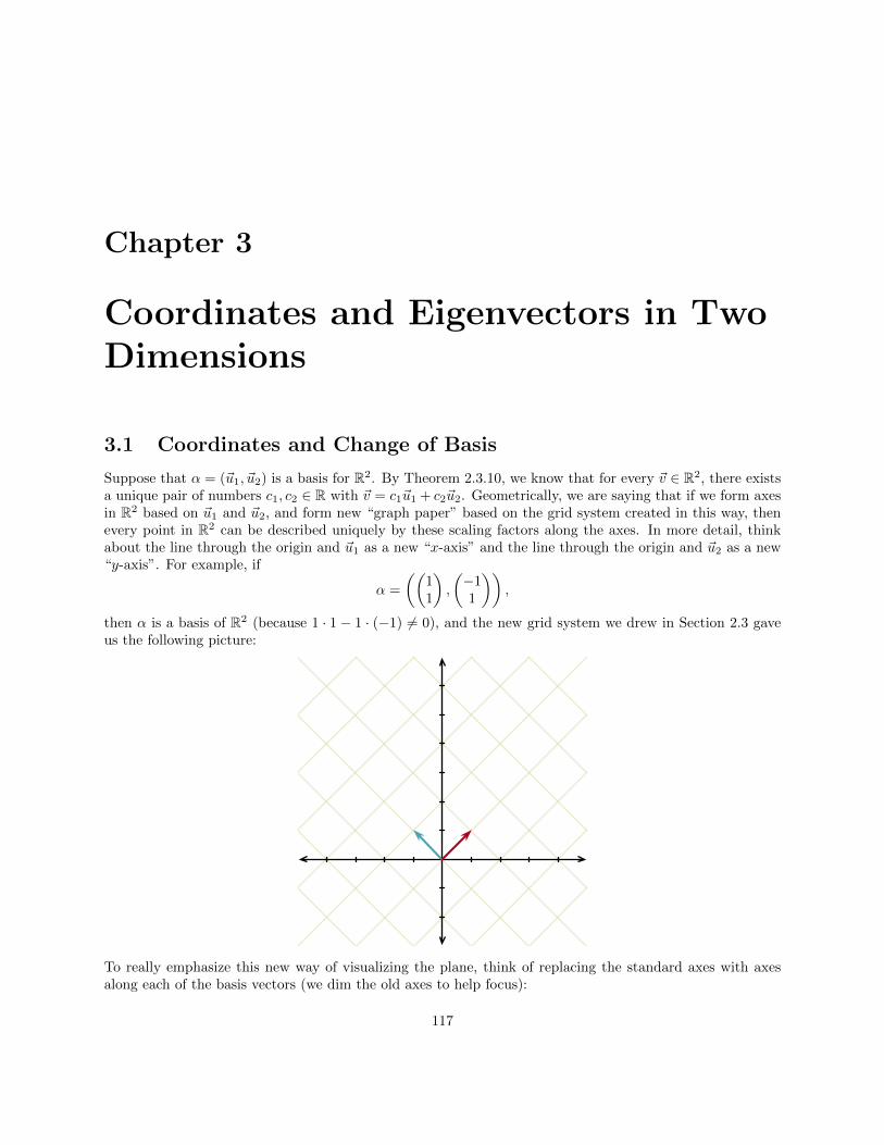
Chapter 3
Coordinates and Eigenvectors in TwoDimensions
3.1 Coordinates and Change of Basis
Suppose that α = (~u1, ~u2) is a basis for R2. By Theorem 2.3.10, we know that for every ~v ∈ R2, there existsa unique pair of numbers c1, c2 ∈ R with ~v = c1~u1 + c2~u2. Geometrically, we are saying that if we form axesin R2 based on ~u1 and ~u2, and form new “graph paper” based on the grid system created in this way, thenevery point in R2 can be described uniquely by these scaling factors along the axes. In more detail, thinkabout the line through the origin and ~u1 as a new “x-axis” and the line through the origin and ~u2 as a new“y-axis”. For example, if
α =
((11
),
(−11
)),
then α is a basis of R2 (because 1 · 1− 1 · (−1) 6= 0), and the new grid system we drew in Section 2.3 gaveus the following picture:
To really emphasize this new way of visualizing the plane, think of replacing the standard axes with axesalong each of the basis vectors (we dim the old axes to help focus):
117
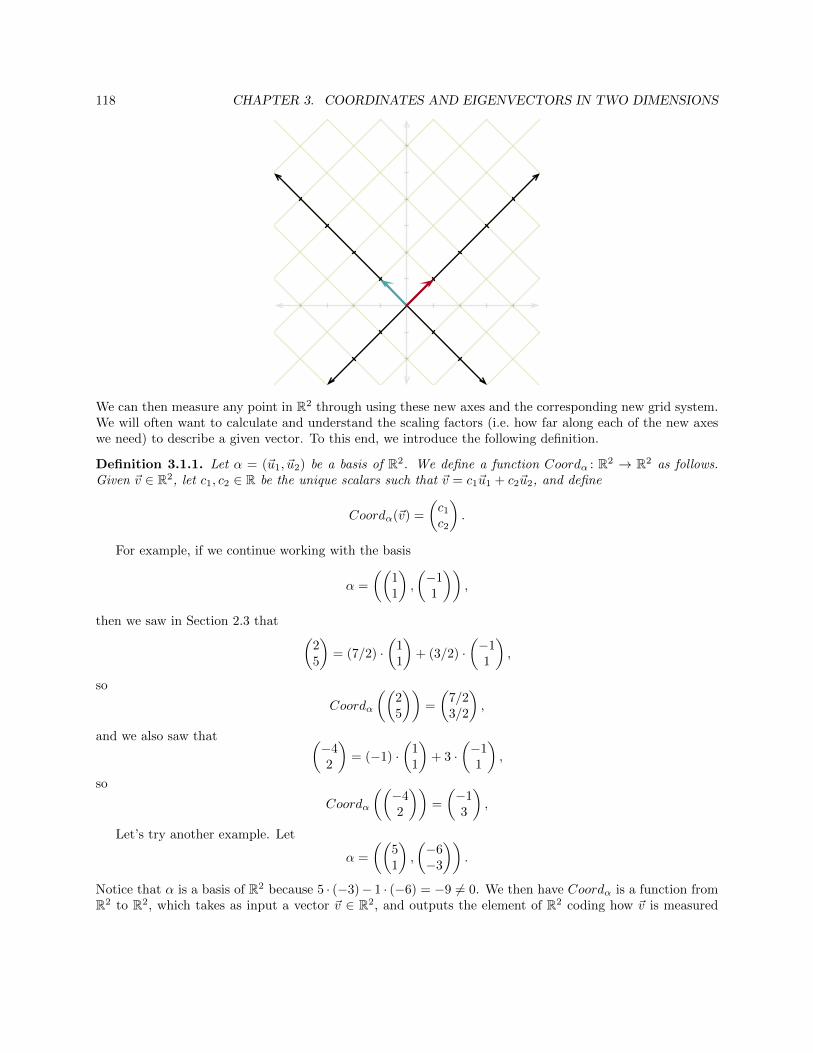
118 CHAPTER 3. COORDINATES AND EIGENVECTORS IN TWO DIMENSIONS
We can then measure any point in R2 through using these new axes and the corresponding new grid system.We will often want to calculate and understand the scaling factors (i.e. how far along each of the new axeswe need) to describe a given vector. To this end, we introduce the following definition.
Definition 3.1.1. Let α = (~u1, ~u2) be a basis of R2. We define a function Coordα : R2 → R2 as follows.Given ~v ∈ R2, let c1, c2 ∈ R be the unique scalars such that ~v = c1~u1 + c2~u2, and define
Coordα(~v) =
(c1c2
).
For example, if we continue working with the basis
α =
((11
),
(−11
)),
then we saw in Section 2.3 that (25
)= (7/2) ·
(11
)+ (3/2) ·
(−11
),
so
Coordα
((25
))=
(7/23/2
),
and we also saw that (−42
)= (−1) ·
(11
)+ 3 ·
(−11
),
so
Coordα
((−42
))=
(−13
),
Let’s try another example. Let
α =
((51
),
(−6−3
)).
Notice that α is a basis of R2 because 5 · (−3)− 1 · (−6) = −9 6= 0. We then have Coordα is a function fromR2 to R2, which takes as input a vector ~v ∈ R2, and outputs the element of R2 coding how ~v is measured
3.1. COORDINATES AND CHANGE OF BASIS 119
in the coordinate system based on α, i.e. how much along the ~u1-axis we need to go (measured in steps oflength equal to the length of ~u1) and how much along the ~u2-axis we need to go. Suppose that we want tocompute
Coordα
((120
)).
In order to do this, we need to find the unique c1, c2 ∈ R with(120
)= c1 ·
(51
)+ c2 ·
(−6−3
).
We find these values by solving the following linear system:
5x − 6y = 12x − 3y = 0.
Solving this system directly, or just applying Proposition 2.1.1, we see that the unique solution is (4, 43 ).Therefore, we have (
120
)= 4 ·
(51
)+ (4/3) ·
(−6−3
).
and hence
Coordα
((120
))=
(4
4/3
).
Using this idea, we can obtain a formula for the function Coordα by applying Proposition 2.1.1.
Proposition 3.1.2. Let α = (~u1, ~u2) be a basis of R2. Fix a, b, c, d ∈ R with
~u1 =
(ac
)and ~u2 =
(bd
).
For any j, k ∈ R, we have
Coordα
((jk
))=
(dj−bkad−bcak−cjad−bc
)
=1
ad− bc·(dj − bkak − cj
)Proof. Let j, k ∈ R be arbitrary. To calculate
Coordα
((jk
)),
we need to find the unique r1, r2 ∈ R with(jk
)= r1 ·
(ac
)+ r2 ·
(bd
).
Finding these values in the same thing as solving the following linear system:
ax + by = jcx + dy = k
120 CHAPTER 3. COORDINATES AND EIGENVECTORS IN TWO DIMENSIONS
Since α is a basis of R2, we know that ad − bc 6= 0 by Theorem 2.3.10. Using Proposition 2.1.1, we knowthat this system has a unique solution, namely(
dj − bkad− bc
,ak − cjad− bc
).
Therefore, we have
Coordα
((jk
))=
(dj−bkad−bcak−cjad−bc
)
=1
ad− bc·(dj − bkak − cj
).
Although this formula certainly works, and is often convenient for short calculations, it is typically bestnot to think of the function Coordα as given by some ugly formula. We will discuss the advantages and dis-advantages of viewing these coordinate changes geometrically, algebraically, and computational throughoutthe course.
Proposition 3.1.3. Let α = (~u1, ~u2) be a basis of R2. The function Coordα : R2 → R2 is a linear transfor-mation.
One way to see this is to use the formula we developed for Coordα in Proposition 3.1.2.
Proof 1 of Proposition 3.1.3. Fix a, b, c, d ∈ R with
~u1 =
(ac
)and ~u2 =
(bd
).
Since α is a basis of R2, we know from Theorem 2.3.10 that ad− bc 6= 0. Now we know that Coordα can bedescribed by the following formula:
Coordα
((xy
))=
(dx−byad−bcay−cxad−bc
).
Rewriting this formula as
Coordα
((xy
))=
(d
ad−bc · x+ −bad−bc · y
−cad−bc · x+ a
ad−bc · y
)= x ·
(d
ad−bc−c
ad−bc
)+ y ·
(−b
ad−bca
ad−bc
),
we can apply Proposition 2.4.3 to immediately conclude that Coordα is a linear transformation.
Although this works, there is a more elegant way to prove this result which avoids ugly formulas and“opening up” the vectors ~u1 and ~u2.
Proof 2 of Proposition 3.1.3. We first check that Coordα preserves addition. Let ~v1, ~v2 ∈ R2 be arbitrary.Since α is a basis of R2, we can apply Theorem 2.3.10 and fix the unique pair of numbers c1, c2 ∈ R and theunique pair of numbers d1, d2 ∈ R with
~v1 = c1~u1 + c2~u2
and~v2 = d1~u1 + d2~u2.
3.1. COORDINATES AND CHANGE OF BASIS 121
By definition of Coordα, we have
Coordα(~v1) =
(c1c2
)and Coordα(~v2) =
(d1d2
).
Notice that
~v1 + ~v2 = c1~u1 + c2~u2 + d1~u1 + d2~u2
= c1~u1 + d1~u1 + c2~u2 + d2~u2
= (c1 + d1)~u1 + (c2 + d2)~u2.
Since c1 +d1 ∈ R and c2 +d2 ∈ R, we have found the (necessarily unique by Theorem 2.3.10) pair of numbersthat express ~v1 + ~v2 as a linear combination of ~u1 and ~u2. Therefore, we have
Coordα(~v1 + ~v2) =
(c1 + d1c2 + d2
)=
(c1c2
)+
(d1d2
)= Coordα(~v1) + Coordα(~v2).
Since ~v1, ~v2 ∈ R2 were arbitrary, it follows that Coordα preserves addition.We now check that Coordα preserves scalar multiplication. Let ~v ∈ R2 and c ∈ R be arbitrary. Since α
is a basis of R2, we can apply Theorem 2.3.10 and fix the unique pair of numbers d1, d2 ∈ R2 with
~v = d1~u1 + d2~u2
By definition of Coordα, we have
Coordα(~v) =
(d1d2
).
Notice that
c~v = c · (d1~u1 + d2~u2)
= c · (d1~u1) + c · (d2~u2)
= (cd1)~u1 + (cd2)~u2.
Since cd1 ∈ R and cd2 ∈ R, we have found the (necessarily unique by Theorem 2.3.10) pair of numbers thatexpress c~v as a linear combination of ~u1 and ~u2. Therefore, we have
Coordα(c~v) =
(cd1cd2
)= c ·
(d1d2
)= c · Coordα(~v).
Since ~v ∈ R2 and c ∈ R were arbitrary, it follows that Coordα preserves scalar multiplication.We’ve shown that Coordα preserves both addition and scalar multiplication, so Coordα is a linear trans-
formation.
For example, since we computed a formula for the functions Coordα, we can immediately determine thestandard matrix of these linear transformations.
122 CHAPTER 3. COORDINATES AND EIGENVECTORS IN TWO DIMENSIONS
Proposition 3.1.4. Let α = (~u1, ~u2) be a basis of R2. If
~u1 =
(ac
)and ~u2 =
(bd
),
then
[Coordα] =
(d
ad−bc−b
ad−bc−c
ad−bca
ad−bc
).
Thus, if we let
P =
(a bc d
),
then [Coordα] = P−1.
Proof. We proved in Proposition 3.1.3 that Coordα is a linear transformation. We also developed a formulafor Coordα in Proposition 3.1.2:
Coordα
((xy
))=
(dx−byad−bcay−cxad−bc
)
=
(d
ad−bc · x+ −bad−bc · y
−cad−bc · x+ a
ad−bc · y
).
Therefore, using Proposition 2.5.8, we can immediately conclude that
[Coordα] =
(d
ad−bc−b
ad−bc−c
ad−bca
ad−bc
).
The last statement is now immediate from Proposition 2.7.9.
For example, suppose that
~u1 =
(12
)and ~u2 =
(37
).
We then have that
[Coordα] =
(1 32 7
)−1=
1
7 · 1− (−3) · (−2)
(7 −3−2 1
)=
(7 −3−2 1
),
so we can compute values of Coordα by simply multiplying by this matrix. In other words, we have
Coordα
((49
))=
(7 −3−2 1
)(49
)=
(7 · 4 + (−3) · 9(−2) · 4 + 1 · 9
)=
(11
).
3.1. COORDINATES AND CHANGE OF BASIS 123
Since we will be changing coordinates a lot in the coming sections, and since the notation Coordα(~v) willbecome cumbersome, we introduce some simplified notation.
Notation 3.1.5. Let α = (~u1, ~u2) be a basis of R2. Given ~v ∈ R2, we use the notation [~v]α as shorthandfor Coordα(~v).
Thus, working with the basis
α =
((11
),
(−11
)),
we can write [(25
)]α
=
(7/23/2
)and [(
−42
)]α
=
(−13
),
With this new notation, we can summarize Proposition 3.1.4 as follows. Given any basis α = (~u1, ~u2) of R2,say
~u1 =
(ac
)and ~u2 =
(bd
),
and we let
P =
(a bc d
),
then we have
[~v]α = P−1~v
for all ~v ∈ R2. In hindsight, we can understand the appearance of the inverse of P both algebraically andgeometrically:
• Algebraic Approach: Suppose that we have a basis α described above, are given some ~v ∈ R2, and are
trying to compute [~v]α. If ~v =
(jk
), then we are tying to find the unique x, y ∈ R with
x ·(ac
)+ y ·
(bd
)=
(jk
),
which means that we are trying to solve the following system of equations:
ax + by = jcx + dy = k.
Using our notation P above for the corresponding matrix, we are trying to find the unique vector~x ∈ R2 with P~x = ~v. As described at the end of Section 2.7, the unique such vector is ~x = P−1~v.Thus, we have [~v]α = P−1~v for all ~v ∈ R2.
• Geometric Approach: Consider the situation from the point of view of the new coordinate system.Suppose we have a vector ~v ∈ R2, and we happen to know for some reason that
[~v]α =
(r1r2
).
124 CHAPTER 3. COORDINATES AND EIGENVECTORS IN TWO DIMENSIONS
Geometrically, we are saying that you get ~v by using r1 and r2 as the scaling factors on each of theaxes in the new coordinate system. More formally, we are saying that
~v = r1 ·(ac
)+ r2 ·
(bd
)=
(a bc d
)(r1r2
).
Thus, for any ~v ∈ R2, we have ~v = P [~v]α. Multiplying both sides by P−1 on the left, it follows that[~v]α = P−1~v for all ~v ∈ R2.
Before moving on, let’s take a moment to reflect on this situation and compare it to similar situationsin the past. In Calculus 2, you saw a different way to describe points in R2 by using polar coordinates.For example, the point (1, 1) in the Cartesian plane can be described by the polar point (
√2, π4 ). In other
words, you already have some experience labeling points in the plane using a pair of numbers different fromthe usual Cartesian pair of numbers. We are doing the same thing now, except in this setting we now haveinfinitely many different coordinate changes: one for each choice of basis α = (~u1, ~u2). However, in manyways our coordinate changes are much better behaved than the polar coordinate changes:
• Geometrically, the grid system formed by our new coordinates consist entirely of parallelograms. Incontrast, in the polar system, the “regions” that we obtain are cut out between circles (for constantvalue of r) and rays from the origin (for constant values of θ). Thus, some of the boundaries in thepolar system are curves rather than straight lines.
• Not only are the regions of the grid system in our new coordinates parallelograms, but in fact theyconsist of repeating parallelograms of precisely the same size and shape throughout the plane. In thepolar system, the regions become larger (for fixed change in r and θ) as we move further from theorigin. In other words, there is a distortion in the polar system that does not arise in our new systems.This “area distortion” is at the root of the r that must be inserted when performing double integralsin polar coordinates, because the regions become scaled by a factor of r depending on the distancefrom the origin. We will begin to discuss this general idea of area distortion when we talk aboutdeterminants.
• In our new coordinate systems, every point can be described by a unique pair of numbers. In contrast,every point has infinitely many polar descriptions. For example, in addition to representing (1, 1) bythe polar point (
√2, π4 ), we can also represent it by the polar point (
√2, 9π4 ), or even by (−
√2, 5π4 ).
Now if we restrict to r ≥ 0 and 0 ≤ θ < 2π, then we fix most of these issues, but the origin can still bedescribed in the infinitely many ways (0, θ) for any value of θ.
3.2 Matrices with Respect to Other Coordinates
Consider the unique linear transformation T : R2 → R2 with standard matrix
[T ] =
(2 11 2
).
Unlike some of the simpler examples that we have seen so far, it is not immediately clear how this transfor-mation acts geometrically on the plane. We can try to plug in points, and perhaps with enough such valueswe might see a pattern. However, it turns out that this linear transformation T can be best understood andvisualized by changing coordinates. That is, instead of looking at the plane as demarcated using the usualCartesian grid system based on ~e1 and ~e2, we can get a much better sense of what is happening by lookingthrough the eyes of somebody using a different grid system.
3.2. MATRICES WITH RESPECT TO OTHER COORDINATES 125
Recall that in our definition of the standard matrix of a linear transformation T , we coded the actionof T based on the values on ~e1 and ~e2. However, if (~u1, ~u2) is a basis of R2, then by Proposition 2.4.4,we know that T is completely determined by its action on ~u1 and ~u2 as well. Furthermore, in conjunctionwith Theorem 2.4.5, we can pick T (~u1) and T (~u2) arbitrarily and there will then be exactly one lineartransformation sending ~u1 and ~u2 to these values. Imagine living a world that has a grid system based on~u1 and ~u2 as the foundation. How would the people living in this world code T as a matrix?
For example, suppose that in this world they are using the two vectors
~u1 =
(3−1
)and ~u2 =
(21
)as the basis of their coordinates. Notice that 3 ·1− (−1) ·2 = 5, which is nonzero, so (~u1, ~u2) is indeed a basisof R2. To us, these two vectors may look like a strange choice, but to the person living in this world theyare simply their versions of ~e1 and ~e2, and they view our choice of two vectors as bizarre. Now if the peoplein this world knew the values T (~u1) and T (~u2), then they could determine the value of T on everything else.More specifically, given ~v ∈ R2, in order to determine T (~v), they would start by finding c1, c2 ∈ R with
~v = c1~u1 + c2~u2.
In other words, they would first determine [~v]α, the coordinates of ~v in their system. Moreover, they wouldliterally view ~v as the vector (
c1c2
)even though we would look at its entries differently (we would open up ~u1 and ~u2, multiply by the constants,and add to obtain the standard coordinates of ~v). From here, they would compute
T (~v) = T (c1~u1 + c2~u2)
= c1 · T (~u1) + c2 · T (~u2)
in order to determine T (~v). Now in our above example with the given T , ~u1, and ~u2, then you might imaginethat such a person would compute as follows:
T (~u1) =
(2 11 2
)(3−1
)=
(51
)T (~u2) =
(2 11 2
)(21
)=
(54
)However, be careful here! We computed these values using the standard matrix of T , which is the matrixof T relative to our coordinates. Just like we do not do yet know the matrix of the people working in adifferent grid system, they do not know our (standard) matrix, so they certainly would not compute in thisway. Moreover, when we write the vectors on the right, we are really thinking about them as(
51
)= 5 · ~e1 + 1 · ~e2,
so by “opening up” these outputs we are looking at them through the tainted eyes of our coordinates!Although the people in this world would not follow our computations, we can still figure out their answer.
How? Well, they are looking to find d1, d2 ∈ R with
T (~u1) = d1~u1 + d2~u2,
126 CHAPTER 3. COORDINATES AND EIGENVECTORS IN TWO DIMENSIONS
i.e. from our perspective they are trying to calculate [T (~u1)]α. Notice that(51
)=
3
5·(
3−1
)+
8
5·(
21
),
or in other words
T (~u1) =3
5· ~u1 +
8
5· ~u2.
Thus, in their coordinates, they would view T (~u1) as the vector(3585
).
Now we also have (54
)= −3
5·(
3−1
)+
17
5·(
21
),
or in other words
T (~u2) = −3
5· ~u1 +
17
5· ~u2.
Thus, in their coordinates, they would view T (~u2) as the vector(− 3
5175
)
Putting it all together, if the people in this world used their coordinates throughout, it looks like they wouldcode T with the matrix (
35 − 3
585
175
).
Here is the general definition.
Definition 3.2.1. Let α = (~u1, ~u2) be a basis of R2, and let T : R2 → R2 be a linear transformation. Fixa, b, c, d ∈ R with
[T (~u1)]α =
(ac
)and
[T (~u2)]α =
(bd
).
We define the matrix of T relative to α to be (a bc d
).
We denote this matrix by [T ]α. In other words, we let the first column of [T ]α be the coordinates of T (~u1)relative to α, and we let the second column of [T ]α be the coordinates of T (~u2) relative to α.
We now prove the following analogue of Proposition 2.5.4 which says that the matrix [T ]α really does codethe transformation correctly from the point of view of people working with α-coordinates throughout. Tosee how these relate, notice that if we let ε = (~e1, ~e2), then we have [~v]ε = ~v for all ~v ∈ R2 and [T ]ε = [T ] forall linear transformations T : R2 → R2, so we can rewrite Proposition 2.5.4 as saying that [T (~v)]ε = [T ]ε · [~v]εfor all linear transformations T : R2 → R2 and all ~v ∈ R2. We now generalize this to any coordinate system.
3.2. MATRICES WITH RESPECT TO OTHER COORDINATES 127
Proposition 3.2.2. Let α = (~u1, ~u2) be a basis of R2, and let T : R2 → R2 be a linear transformation. Wehave
[T (~v)]α = [T ]α · [~v]α
for all ~v ∈ R2.
Proof. Fix a, b, c, d ∈ R with
[T ]α =
(a bc d
).
Now let ~v ∈ R2 be arbitrary. Fix r1, r2 ∈ R with
[~v]α =
(r1r2
).
By definition, we then have ~v = r1 · ~u1 + r2 · ~u2. Since T is a linear transformation, notice that
T (~v) = T (r1 · ~u1 + r2 · ~u2)
= r1 · T (~u1) + r2 · T (~u2).
Now using the fact that Coordα is a linear transformation from Proposition 3.1.3, we have
[T (~v)]α = [r1 · T (~u1) + r2 · T (~u2)]α
= r1 · [T (~u1)]α + r2 · [T (~u2)]α
= r1 ·(ac
)+ r2 ·
(bd
)=
(a bc d
)(r1r2
)= [T ]α · [~v]α.
Let’s see this result in action with the T and α = (~u1, ~u2) that we have been using, i.e. with
[T ] =
(2 11 2
), ~u1 =
(3−1
), and ~u2 =
(21
).
Let
~v =
(105
).
In the standard coordinate system, we have
T (~v) =
(2 11 2
)(105
)=
(2520
).
Now notice that
~v = 0 · ~u1 + 5 · ~u2,
so in α coordinate system, we have
[~v]α =
(05
).
128 CHAPTER 3. COORDINATES AND EIGENVECTORS IN TWO DIMENSIONS
Thus, to determine [T (~v)]α, people living in the α-coordinate world would compute
[T (~v)]α =
(35 − 3
585
175
)(0
5
)=
(−3
17
).
Don’t be alarmed that these results look different! After all, we have
−3 ·(
3−1
)+ 17 ·
(21
)=
(2520
)= 25 ·
(10
)+ 20 ·
(01
),
so we of course get the same answer, just viewed through the lens of different coordinate systems.
Let’s recap the process for computing [T ]α given a basis α = (~u1, ~u2). Compute T (~u1), but rather thanuse the two numbers inside this vector (which are really the coordinates relative to ~e1 and ~e2), instead findthe unique c1, c2 ∈ R with
T (~u1) = c1~u1 + c2~u2.
Similarly, find the unique d1, d2 ∈ R with
T (~u2) = d1~u1 + d2~u2.
We then have that
[T ]α =
(c1 d1c2 d2
).
At this point, you may ask yourself a very reasonable question. We started with a linear transformationT : R2 → R2 with
[T ] =
(2 11 2
).
We looked at a new coordinate system α and found that
[T ]α =
(35 − 3
585
175
).
So we replaced a matrix that we did not understand geometrically by a much uglier matrix that we do notunderstand geometrically. What progress! In this case, it is correct to say that this coordinate system madethings worse. However, let’s try a different coordinate system. Suppose that we let
~w1 =
(11
)and ~w2 =
(−11
),
and let β = (~w1, ~w2). We have that β is a basis of R2 because 1 · 1− 1 · (−1) = 2 is nonzero. Notice that
T (~w1) =
(2 11 2
)(11
)=
(33
)= 3 ·
(11
)+ 0 ·
(−11
)= 3 · ~w1 + 0 · ~w2
3.2. MATRICES WITH RESPECT TO OTHER COORDINATES 129
so
[T (~w1)]β =
(30
).
Also, we have
T (~w2) =
(2 11 2
)(−11
)=
(−11
)= 0 ·
(11
)+ 1 ·
(−11
)= 0 · ~w1 + 1 · ~w2,
so
[T (~w2)]β =
(01
).
It follows that
[T ]β =
(3 00 1
).
Now this is a much simpler matrix to think about! In the standard coordinates, this matrix expands theplane horizontally by a factor of 3 because(
3 00 1
)(c1c2
)=
(3c1c2
)for all c1, c2 ∈ R. In other words, if a point is a distance of c1 away from the y-axis, then it stays on thesame horizontal line but is now 3 times as far from the y-axis. The same matrix-vector calculation applieshere, but we just need to interpret it differently. Instead of thinking about c1 and c2 as the distances alongthe x-axis and y-axis that we travel (i.e. the amount we scale ~e1 and ~e2 by), we instead think about them asthe amount we scale ~w1 and ~w2 by. In other words, we have
T (c1 · ~w1 + c2 · ~w2) = 3c1 · ~w1 + c2 · ~w2
for all c1, c2 ∈ R. It follows that our transformation is an expansion by a factor of 3, but parallel to adifferent line than the x-axis. Notice that Span(~w1) is the solution set to y = x, and Span(~w2) is the solutionset to y = −x. Thus, our grid system consists of lines parallel to y = x or y = −x. From this perspective,our transformation takes a point, and triples the amount it has along the line y = x, while keeping the sameamount it has along the line y = −x. Since y = x and y = −x are perpendicular, we can view T as simplyexpanding the plane by a factor of 3 in a perpendicular direction away from the line y = −x.
As we’ve just witnessed, by using a change in coordinates, we can sometime understand the action ofa linear transformation more deeply. However, there are several questions that remain. How do we find agood coordinate system so that the matrix is “simple”? How are the matrices between different coordinatesystems related? Can we compute these matrices more quickly? We will answer the latter two questions inthis section, and begin to answer the first (and probably most important) question in the next section. Itturns out that answering the first question definitively is quite difficult, and the situation in more than twodimensions is beyond the scope of a first course.
Suppose then that T : R2 → R2 is a linear transformation. Let α = (~u1, ~u2) be a basis of R2. For somesimplified notation without square brackets, let A = [T ], let B = [T ]α, and let C = [Coordα]. How do
130 CHAPTER 3. COORDINATES AND EIGENVECTORS IN TWO DIMENSIONS
A and B relate to each other? The matrix C takes a vector in standard coordinates and converts it intoα-coordinates, and we can then feed that output into B to get the result of T (~v) in α-coordinates (usingProposition 3.2.2). In other words, BC takes a vector ~v and outputs [T (~v)]α. For the other product, A takesa vector in standard coordinates and outputs T (~v) in standard coordinates, which we can feed into C to getthe α coordinates of T (~v), i.e. to get [T (~v)]α. Since these are the same, it looks like given any ~v ∈ R2, wecan follow the diagram below in either direction to arrive at the same result:
~v → C → [~v]α↓ ↓A B↓ ↓
T (~v) → C → [T (~v)]α
In other words, it appears that (CA)~v = (BC)~v for all ~v ∈ R2. We now prove this.
Proposition 3.2.3. Let α = (~u1, ~u2) be a basis of R2 and let T : R2 → R2 be a linear transformation. LetA = [T ], let B = [T ]α, and let C = [Coordα]. We then have that (CA)~v = (BC)~v for all ~v ∈ R2.
Proof. For any ~v ∈ R2, we have
(CA)~v = C(A~v)
= C · T (~v)
= [T (~v)]α
= [T ]α · [~v]α (by Proposition 3.2.2)
= B · [~v]α
= B(C~v)
= (BC)~v.
In general, if two matrices act the same on all vectors, they they must be the same matrix.
Proposition 3.2.4. Let A and B be 2× 2 matrices. If A~v = B~v for all ~v ∈ R2, then A = B.
Proof. Exercise.
Corollary 3.2.5. Let α = (~u1, ~u2) be a basis of R2 and let T : R2 → R2 be a linear transformation. LetA = [T ], let B = [T ]α, and let C = [Coordα]. We then have that CA = BC.
Proof. This follows immediately from Proposition 3.2.3 and Proposition 3.2.4.
We can now use the formula for [Coordα] that we developed in Proposition 3.1.4 in order to establish astraightforward way to compute [T ]α from [T ].
Proposition 3.2.6. Let α = (~u1, ~u2) be a basis of R2 and let T : R2 → R2 be a linear transformation. Fixa, b, c, d ∈ R with
~u1 =
(ac
)and ~u2 =
(bd
)and notice that ad− bc 6= 0 (because α is a basis of R2). Let
P =
(a bc d
).
We then have that P is invertible and[T ]α = P−1[T ]P.
3.2. MATRICES WITH RESPECT TO OTHER COORDINATES 131
Proof. Let A = [T ], let B = [T ]α, and let C = [Coordα]. We know Corollary 3.2.5 that CA = BC. NowProposition 3.1.4 tells us that C = P−1, so P−1A = BP−1. Multiplying both sides of this equation on theright by P , we conclude that P−1AP = B, i.e. that [T ]α = P−1[T ]P .
Let’s take a step back and interpret what this is saying. Suppose that α = (~u1, ~u2) and P are as in thesetup of the proposition. We are claiming that
[T ]α =
(a bc d
)−1· [T ] ·
(a bc d
).
How does this work? Suppose that we are given a vector ~v and its α-coordinates are
[~v]α =
(xy
).
When we feed this vector [~v]α as input to the matrix P on the right, we get as output
(a bc d
)(xy
)= x ·
(ac
)+ y ·
(bd
),
which when expanded out will give us the standard coordinates for ~v. When we feed this result into thematrix [T ], we see that it gets transformed into T (~v) in standard coordinates. We then go ahead and feedthis result into the matrix P−1 = C on the left, which takes T (~v) in standard coordinates and turns into[T (~v)]α, i.e. the α-coordinates of T (~v). In other words, the chaining of three matrices on the right convertsα-coordinates to standard coordinates, then transforms this result in standard coordinates, then convertsfrom standard coordinates to α-coordinates, and this three-step process can also be accomplished by justusing the matrix [T ]α alone.
With this result in hand, we now have a significantly easier way to compute the matrix [T ]α using [T ]and the two vectors ~u1 and ~u2. To see this in action, let’s go back to our original example in this section.So let T : R2 → R2 be the unique linear transformation with
[T ] =
(2 11 2
)
and let α = (~u1, ~u2) where
~u1 =
(3−1
)and ~u2 =
(21
).
Letting
P =
(3 2−1 1
),
we have
P−1 =1
5
(1 −21 3
),
132 CHAPTER 3. COORDINATES AND EIGENVECTORS IN TWO DIMENSIONS
hence
[T ]α = P−1AP
=1
5
(1 −21 3
)(2 11 2
)(3 2−1 1
)=
1
5
(1 −21 3
)(5 51 4
)=
1
5
(3 −38 17
)=
(35
−35
85
175
),
as we calculated above. Again, the advantage of this approach over our previous methods is that we cansimply invert a matrix and perform a straightforward computation without having to think through theconcepts every single time.
For the other coordinate system, consider β = (~w1, ~w2) where
~w1 =
(11
)and ~w2 =
(−11
).
Letting
P =
(1 −11 1
),
we have
P−1 =1
2
(1 1−1 1
),
hence
[T ]β = P−1[T ]P
=1
2
(1 1−1 1
)(2 11 2
)(1 −11 1
)=
1
2
(1 1−1 1
)(3 −13 1
)=
1
2
(6 00 2
)=
(3 00 1
),
as we calculated above.
We end with a new example. Consider the unique linear transformation T : R2 → R2 with
[T ] =
(43
16
− 23
23
).
As in our previous example, this matrix is sufficiently complicated that it seems extremely difficult to viewthe corresponding action geometrically. However, consider the following coordinate system. Let α = (~u1, ~u2)where
~u1 =
(1−2
)and ~u2 =
(30
).
3.2. MATRICES WITH RESPECT TO OTHER COORDINATES 133
Letting
P =
(1 3−2 0
),
we have
P−1 =1
6
(0 −32 1
),
hence
[T ]α = P−1[T ]P
=1
6
(0 −32 1
)( 43
16
− 23
23
)(1 3
−2 0
)
=1
6
(0 −32 1
)(1 4−2 −2
)=
1
6
(6 60 6
)=
(1 10 1
).
Aha, this is a matrix that we understand! In standard coordinates, it represents a horizontal shear relativeto the x-axis, i.e. it shifts the half-plane above the x-axis to the right, and shifts the half-plane below thex-axis to the left. The underlying reason for this is that(
1 10 1
)(xy
)=
(x+ yy
)for all x, y ∈ R. Thus, every point on the line y = 0 (which is Span(~e1)) is fixed, the line y = 1 is shifted tothe right by 1, the line y = 3 is shifted to the right by 3, the line y = −2 is shifted to the left by 2, etc.
However, we have to geometrically interpret our matrix differently because it is in α-coordinates. Al-though the vectors ~u1 and ~u2 are not perpendicular, we still obtain a certain kind of shear transformation.Notice that the above matrix tells us that if ~v has α-coordinates(
c1c2
)then T (~v) will have α-coordinates (
c1 + c2c2
).
In other words, we have
T (c1 · ~u1 + c2 · ~u2) = (c1 + c2) · ~u1 + c2 · ~u2
for all c1, c2 ∈ R. Thus, instead of the shear being relative to the line y = 0, which is Span(~e1), it will berelative to Span(~u1), i.e. relative to the line y = −2x. All points on this line are fixed because the secondα-coordinate of such a point is 0. Every point with second α-coordinate equal to 1, i.e. every point that is 3to the right of the line y = −2x, will have its first α-coordinate shifted by 1. In other words, points on theline y = −2(x− 3) = −2x+ 6 will stay on this line, but will move down along it by adding ~u1. Continuingin this way, anything to the right of the line y = −2x will be sheared in the direction of ~u1 by an amountproportional to its horizontal distance from y = −2x, and anything to the left of the line y = −2x will besheared in the direction of −~u1 by an amount proportional to its horizontal distance from y = −2x.
134 CHAPTER 3. COORDINATES AND EIGENVECTORS IN TWO DIMENSIONS
3.3 Eigenvalues and Eigenvectors
In the previous section, we learned how a well-chosen change in coordinates can produce a simpler matrixfor a linear transformation T , which can lead to both geometric and algebraic understanding of how T acts.However, we gave no indication of how to choose α = (~u1, ~u2) in a way so that [T ]α is “nice”. In this section,we first define what we consider ”nice” behavior, and then explore how to find bases α such that [T ]α willbe as simple as possible.
In our first example in the previous section, where
[T ] =
(2 11 2
),
we worked with β = (~w1, ~w2) where
~w1 =
(11
)and ~w2 =
(−11
).
For this choice of coordinates, we have
[T ]β =
(3 00 1
).
In other words, we have T (~w1) = 3~w1 and T (~w2) = ~w2. This latter equation where we found a fixed pointof T looks ideal. What could be better than a point that is not moved by T? The former equation is almostas good. We have that T (~w1) is simply stretched, and so the result is that T (~w1) is still an element ofSpan(~w1). In other words, although ~w1 was moved, it was not rotated in any way, and hence was sent toanother point in Span(~w1). We now give a name to the points and scaling factors that arise in this way.
Definition 3.3.1. Let T : R2 → R2 be a linear transformation.
• An eigenvector of T is a nonzero vector ~v ∈ R2 such that there exists λ ∈ R with T (~v) = λ~v.
• An eigenvalue of T is a scalar λ ∈ R such that there exists a nonzero ~v ∈ R2 with T (~v) = λ~v.
When ~v ∈ R2 is nonzero and λ ∈ R are such that T (~v) = λ~v, we say that ~v is an eigenvector of Tcorresponding to the eigenvalue λ.
For example, suppose that T : R2 → R2 is the unique linear transformation with
[T ] =
(4 −21 1
).
Notice that
T
((21
))=
(4 −21 1
)(21
)=
(63
)= 3 ·
(21
),
so
(21
)is an eigenvector of T , 3 is an eigenvalue of T , and hence
(21
)is an eigenvector of T corresponding
to 3. In contrast, we have
T
((1−3
))=
(4 −21 1
)(1−3
)=
(10−2
).
3.3. EIGENVALUES AND EIGENVECTORS 135
Since there does not exist λ ∈ R with (10−2
)= λ ·
(1−3
)(by contradiction, since such a λ would have to satisfy both λ = 10 and λ = 2
3 ), it follows that
(1−3
)is not
an eigenvector of A.Notice that, in the definition, we insist that an eigenvector ~v is nonzero. One reason for this is that
T (~0) = ~0 for every linear transformation T , so always having a “trivial” eigenvector cheapens the name.More importantly, since T (~0) = ~0, we have that T (~0) = λ · ~0 for every λ ∈ R. Thus, if we do not rule outthe zero vector, then every real number would become an eigenvalue, which we certainly do not want to bethe case.
However, it is possible that 0 could be an eigenvalue for a linear transformation T : R2 → R2. For thisto happen, we just need there to exist a nonzero vector ~v ∈ R2 with T (~v) = ~0, which is the same thing assaying that Null(T ) 6= {~0}. For example, if T : R2 → R2 consider the unique linear transformation with
[T ] =
(1 11 1
).
Notice that Null(T ) 6= {~0} by Theorem 2.7.3 because 1 · 1− 1 · 1 = 0. In fact, we have
T
((1−1
))=
(1 11 1
)(1−1
)=
(00
)= 0 ·
(1−1
).
so
(1−1
)is an eigenvector corresponding to 0. We will see a close relationship between eigenvalues, eigen-
vectors, and null spaces more generally below.
Before moving on, we first show that every eigenvector corresponds to exactly one eigenvalue. As men-tioned above, for this to be true, it is essential that we not allow the zero vector in our definition ofeigenvector.
Proposition 3.3.2. Let T : R2 → R2 be a linear transformation. If ~v is an eigenvector of T , then thereexists a unique λ ∈ R such that ~v is an eigenvector of T corresponding to λ. In other words, if ~v is aneigenvector of T corresponding to both λ ∈ R and µ ∈ R, then λ = µ.
Proof. Let ~v be an eigenvector of T . Suppose that ~v is an eigenvector of T corresponding to both λ ∈ Rand µ ∈ R. By definition of an eigenvector, we then have that ~v 6= ~0, that T (~v) = λ~v, and that T (~v) = µ~v.Combining these latter two equalities, we have λ~v = µ~v, and subtracting µ~v from both sides, we concludethat λ~v − µ~v = ~0. It follows that (λ − µ)~v = ~0. Now if λ − µ 6= 0, then we can divide both sides by λ − µto conclude that ~v = ~0, which would be a contradiction. Therefore, we must have λ − µ = 0, and henceλ = µ.
We have defined eigenvalues and eigenvectors for a linear transformation T , but we can also definethem for matrices. Since matrices code linear transformations, you might think that there is no distinction.However, we do want to keep a sharp distinction between linear transformations and the matrices that codethem because we need both a linear transformation and an α to build a matrix. In particular, one lineartransformation can be represented by distinct matrices when we change the coordinate system. Nonetheless,we can also define these concepts for matrices in the completely analogous way.
136 CHAPTER 3. COORDINATES AND EIGENVECTORS IN TWO DIMENSIONS
Definition 3.3.3. Let A be a 2× 2 matrix.
• An eigenvector of A is a nonzero vector ~v ∈ R2 such that there exists λ ∈ R with A~v = λ~v.
• An eigenvalue of A is a scalar λ ∈ R such that there exists a nonzero ~v ∈ R2 with A~v = λ~v.
When ~v ∈ R2 is nonzero and λ ∈ R are such that A~v = λ~v, we say that ~v is an eigenvector of A correspondingto the eigenvalue λ.
Now if we work with the standard matrix of a linear transformation T : R2 → R2, then it is immediatefrom the definitions that ~v is an eigenvector of T corresponding to λ if and only if ~v an eigenvector of [T ]corresponding to λ. However, if we use a different matrix representation, then the eigenvectors might change.We will not dwell on these issues now, but they will a play a role later.
Let T : R2 → R2 be a linear transformation, and let A = [T ]. Given ~v ∈ R2 and λ ∈ R, it is easy todetermine if ~v is an eigenvector of T corresponding to λ: just calculate A~v and check if it equals λ~v. Now ifwe are only given ~v ∈ R2 (so no λ), it is still straightforward to determine if ~v is an eigenvector of T . Wejust need to compute A~v and then check if the result is some scalar multiple of ~v. However, given λ ∈ R, itis not obvious how we can check whether λ is an eigenvalue and, if so, find eigenvectors corresponding to it.In other words, we have the following two questions:
• Given a real number λ, how do we determine if λ is an eigenvalue of A?
• Given an eigenvalue λ of A, how do we determine the eigenvectors corresponding to λ?
Here is an idea for how to answer the first question. Given λ ∈ R, we want to know if there are any nonzerovectors ~v ∈ R2 such that A~v = λ~v. Intuitively, we want to “solve” for ~v here. To make this happen, we tryto bring the ~v’s together to the other side and instead work with A~v − λ~v = ~0. Now the natural idea is totry to fact out the common ~v, but A− λ does not make sense because we can not subtract a number from amatrix. However, there is a hack to get around this. We can view the scalar multiplication λ~v as a certainmatrix-vector product. For example, if we want to multiply ~v by 5, we can instead hit ~v by the matrix(
5 00 5
).
In other words, we can simply write λ~v as λI~v. Since I is the identity matrix, this is just like multiplyingby 1 in an algebraic equation. With this perspective, we can rewrite A~v − λ~v = ~0 as A~v − λI~v = ~0. Fromhere, we can factor out the ~v and rewrite this as (A−λI)~v = ~0. Thus, to determine if there are any nonzerovectors ~v with A~v = λ~v, we can instead determine if the matrix A−λI kills off any nonzero vectors. In otherwords, we are asking if the null space of the matrix A−λI is nontrivial. We now formalize this argument inthe following result.
Proposition 3.3.4. Let A be a 2 × 2 matrix, let ~v ∈ R2, and let λ ∈ R. We have that A~v = λ~v if andonly if ~v ∈ Null(A − λI). Therefore, ~v is an eigenvector of A corresponding to λ if and only if ~v 6= ~0 and~v ∈ Null(A− λI).
Proof. Suppose first that A~v = λ~v. Subtracting λ~v from both sides, we then have A~v − λ~v = ~0, and henceA~v − λI~v = ~0. We then have (A− λI)~v = ~0, and thus ~v ∈ Null(A− λI).
Conversely, suppose that ~v ∈ Null(A − λI). We then have (A − λI)~v = ~0, so A~v − λI~v = ~0, and henceA~v − λ~v = ~0. Adding λ~v to both sides, we conclude that A~v = λ~v.
From this result, we immediately obtain the following corollary.
Corollary 3.3.5. Let A be a 2× 2 matrix and let λ ∈ R. We have that λ is an eigenvalue of A if and onlyif Null(A− λI) 6= {~0}.
3.3. EIGENVALUES AND EIGENVECTORS 137
Combining this fact with Theorem 2.7.3, we obtain a method to determine if a given number λ ∈ R isan eigenvalue of a matrix A. For example, suppose that we are working with the matrix
A =
(4 −21 1
)as above. Is 5 an eigenvalue of A? We calculate
A− 5I =
(4 −21 1
)−(
5 00 5
)=
(−1 −21 −4
).
Notice that Null(A − 5I) = {~0} by Theorem 2.7.3 because (−1) · (−4) − (−2) · 1 = 6 is nonzero. UsingCorollary 3.3.5, it follows that 5 is not an eigenvalue of A. Now we noticed that 3 was an eigenvalue of Aabove by stumbling across a particular eigenvector corresponding to 3. We can see that 3 is an eigenvaluein another way now. Notice that
A− 3I =
(4 −21 1
)−(
3 00 3
)=
(1 −21 −2
).
Notice that Null(A − 3I) 6= {~0} by Theorem 2.7.3 because (−1) · (−2) − (−2) · 1 = 0. Therefore, 3 is aneigenvalue of A by Corollary 3.3.5. Now if we want to find all eigenvectors corresponding to 3, we just wantto find the null space of the matrix
A− 3I =
(1 −21 −2
).
Following the proof of Theorem 2.7.3 (in Case 3 at the end), we conclude that
Null(A− 3I) = Span
((21
)).
Thus, we rediscover the eigenvector (21
)that we stumbled across above, and in fact any constant multiple of this eigenvector is also an eigenvectorcorresponding to 3. In other words, every element of
Span
((21
))is an eigenvector of A corresponding to 3.
Given a matrix A and a scalar λ ∈ R, we now have a procedure to determine if λ is an eigenvalue of A.Using this, we can go through numbers one at time, and if we’re lucky, we might find eigenvalues. Is there abetter way to find all of the eigenvalues simultaneously? The key fact is that we perform the same procedureno matter what λ is, and so we can simply look at the matrix A − λI in general, and work with it (i.e. wedo not plug a specific value in for λ). Suppose then that
A =
(a bc d
)and we want to find all eigenvalues of A. In other words, we want to find those λ ∈ R such that Null(A−λI) 6={~0}. We have
A− λI =
(a bc b
)−(λ 00 λ
)=
(a− λ bc d− λ
).
138 CHAPTER 3. COORDINATES AND EIGENVECTORS IN TWO DIMENSIONS
Therefore, using Theorem 2.7.3, we have that Null(A − λI) 6= {~0} if and only if (a − λ)(d − λ) − bc = 0.When we expand this out, we obtain a degree two polynomial in the variable λ. We give this polynomial aspecial name.
Definition 3.3.6. Given a 2× 2 matrix
A =
(a bc d
),
we define the characteristic polynomial of A to be the following polynomial in variable λ:
(a− λ)(d− λ)− bc = λ2 − (a+ d)λ+ (ad− bc).
Let’s see a few examples.
Example 3.3.7. Let
A =
(4 −21 1
).
Find all eigenvalues of A, and then find at least one eigenvector of A corresponding to each eigenvalue.
Solution. For any λ ∈ R, we have
A− λI =
(4− λ −2
1 1− λ
),
so the characteristic polynomial of A is
(4− λ)(1− λ)− (−2) = 4− 5λ+ λ2 + 2
= λ2 − 5λ+ 6
= (λ− 3)(λ− 2).
Therefore, Null(A− λI) 6= {~0} if and only either λ = 3 or λ = 2. It follows that the eigenvalues of A are 3and 2. We have already seen that (
21
)is an eigenvector corresponding to 3, and that the set of all eigenvectors corresponding to 3 is
Null(A− 3I) = Span
((21
)).
Now consider λ = 2. We have
A− 2I =
(2 −21 −1
).
To find an eigenvector corresponding to 2, we need only find a nonzero element of the null space of thismatrix. One example is (
11
).
Following the proof of Theorem 2.7.3, we conclude that the set of all eigenvectors corresponding to 3 is
Null(A− 2I) = Span
((11
)).
3.3. EIGENVALUES AND EIGENVECTORS 139
Example 3.3.8. Let
A =
(5 4−7 −6
).
Find all eigenvalues of A, and then find at least one eigenvector of A corresponding to each eigenvalue.
Solution. For any λ ∈ R, we have
A− λI =
(5− λ 4−7 −6− λ
),
so the characteristic polynomial of A is
(5− λ)(−6− λ)− (−28) = −30 + λ+ λ2 + 28
= λ2 + λ− 2
= (λ− 1)(λ+ 2)
Therefore, Null(A− λI) 6= {~0} if and only if either λ = 1 or λ = −2. It follows that the eigenvalues of A are1 and −2. For λ = 1, we have
A− 1I =
(4 4−7 −7
).
To find an eigenvector corresponding to 1, we need only find a nonzero element of the null space of thismatrix. One example is (
−11
).
Following the proof of Theorem 2.7.3, we conclude that the set of all eigenvectors corresponding to 1 is
Null(A− 1I) = Span
((−11
)).
Now consider λ = −2. We have
A+ 2I =
(7 4−7 −4
).
To find an eigenvector corresponding to −2, we need only find a nonzero element of the null space of thismatrix. One example is (
−47
).
Again, following the proof of Theorem 2.7.3, we conclude that the set of all eigenvectors corresponding to−2 is
Null(A+ 2I) = Span
((− 4
71
)).
Example 3.3.9. Let
A =
(0 −11 0
).
Find all eigenvalues of A, and then find at least one eigenvector of A corresponding to each eigenvalue.
140 CHAPTER 3. COORDINATES AND EIGENVECTORS IN TWO DIMENSIONS
Solution. For any λ ∈ R, we have
A− λI =
(−λ −11 −λ
),
so the characteristic polynomial of A is
(−λ)(−λ)− (−1) = λ2 + 1.
Therefore, A has no eigenvalues because λ2 + 1 has no roots in R.
Example 3.3.10. Let
A =
(1 10 1
)Find all eigenvalues of A, and then find at least one eigenvector of A corresponding to each eigenvalue.
Solution. For any λ ∈ R, we have
A− λI =
(1− λ 1
0 1− λ
)so the characteristic polynomial of A is
(1− λ)2 − 0 = (λ− 1)2,
Therefore, 1 is the only eigenvalue of A. We have
A− 1I =
(0 10 0
),
Notice that (10
)is an element of Null(A− 1I), so is an eigenvector of A corresponding to 1. Following the proof of Theorem2.7.3, we conclude that the set of all eigenvectors corresponding to 1 is
Null(A− 1I) = Span
((10
)).
Let’s go back to our matrix
A =
(4 −21 1
).
We know that there exists a unique linear transformation T : R2 → R2 such that [T ] = A. Our originalmotivation for eigenvectors was that they appeared to be smart choices to use as vectors for a new coordinatesystem. Let’s go ahead and make use of that now. We know from Example 3.3.7 that the eigenvalues of Tare 3 and 2. We also know that (
21
)is an eigenvector corresponding to 3, and that (
11
)
3.3. EIGENVALUES AND EIGENVECTORS 141
is an eigenvector corresponding to 2. With this in mind, let α = (~u1, ~u2) where
~u1 =
(21
)and ~u2 =
(11
).
Since 2 · 1− 1 · 1 = 1 is nonzero, we know that (~u1, ~u2) is a basis of R2. Now using the fact that ~u1 and ~u2are eigenvectors of T , we have
T (~u1) = 3~u1
= 3 · ~u1 + 0 · ~u2,
so
[T (~u1)]α =
(30
).
We also have
T (~u2) = 2~u2
= 0 · ~u1 + 2 · ~u2.
so
[T (~u2)]α =
(02
).
It follows that
[T ]α =
(3 00 2
).
Thus, we have indeed found a coordinate system α where [T ]α is particularly nice. We can also compute[T ]α using Proposition 3.2.6. Letting
P =
(2 11 1
)we then have that P is invertible and that
P−1 =
(1 −1−1 2
).
Therefore, we have
[T ]α = P−1 · [T ] · P
=
(1 −1−1 2
)(4 −21 1
)(2 11 1
)=
(1 −1−1 2
)(6 23 2
)=
(3 00 2
).
The reason why we use eigenvectors of T for our choice of ~u1 and ~u2 in our basis α = (~u1, ~u2) is that wealways obtain a matrix that looks like this.
Definition 3.3.11. A diagonal 2× 2 matrix is a 2× 2 matrix D such that there exists a, d ∈ R with
D =
(a 00 d
)
142 CHAPTER 3. COORDINATES AND EIGENVECTORS IN TWO DIMENSIONS
In other words, a diagonal matrix is a matrix that has 0’s off of the main diagonal, but may have nonzeroentries on the main diagonal.
Definition 3.3.12. A linear transformation T : R2 → R2 is diagonalizable if there exists a basis α = (~u1, ~u2)of R2 such that [T ]α is a diagonal matrix.
For example, if T : R2 → R2 is the unique linear transformation with
[T ] =
(4 −21 1
)then we’ve just seen that T is diagonalizable. We now argue generally that a linear transformation isdiagonalizable if and only if we can find a basis of two eigenvectors.
Proposition 3.3.13. Let T : R2 → R2 be a linear transformation and let α = (~u1, ~u2) be a basis of R2. Thefollowing are equivalent:
1. [T ]α is a diagonal matrix.
2. ~u1 and ~u2 are eigenvectors of T .
Furthermore, in this case, the diagonal entries of [T ]α are the eigenvalues corresponding to ~u1 and ~u2, i.e. theupper left entry of [T ]α is the eigenvalue of [T ] corresponding to ~u1, and the lower right entry of [T ]α is theeigenvalue of T corresponding to ~u2.
Proof. Suppose first that [T ]α is a diagonal matrix. Fix a, d ∈ R with
[T ]α =
(a 00 d
).
By the definition of [T ]α, we then have that
T (~u1) = a · ~u1 + 0 · ~u2= a · ~u1,
so ~u1 is an eigenvector corresponding to a. Similarly, we have
T (~u2) = 0 · ~u1 + d · ~u2= d · ~u2,
so ~u2 is an eigenvector corresponding to d. Thus, we have shown that 2 is true, and also the additionalstatement.
Suppose now that ~u1 and ~u2 are eigenvectors of T . Fix λ1, λ2 ∈ R with T (~u1) = λ1 ·~u1 and T (~u2) = λ2 ·~u2.We then have
T (~u1) = λ1 · ~u1= λ1 · ~u1 + 0 · ~u2,
so
[T (~u1)]α =
(λ10
).
We also have
T (~u2) = λ2 · ~u2= 0 · ~u1 + λ2 · ~u2,
3.3. EIGENVALUES AND EIGENVECTORS 143
so
[T (~u1)]α =
(0λ2
).
Therefore, by then definition of [T ]α, we have
[T ]α =
(λ1 00 λ2
).
Thus, we have shown that 1 is true, and also the additional statement.
Corollary 3.3.14. A linear transformation T : R2 → R2 is diagonalizable if and only if there exists a basis(~u1, ~u2) of R2 such that both ~u1 and ~u2 are eigenvectors of T .
Proof. This follows immediately from Proposition 3.3.13.
Example 3.3.15. Let T : R2 → R2 be the unique linear transformation with
[T ] =
(2 −32 −5
).
Determine if T is diagonalizable, and if so, find α such that [T ]α is a diagonal matrix.
Solution. Let A = [T ]. For any λ ∈ R, we have
A− λI =
(2− λ −3
2 −5− λ
),
so the characteristic polynomial of A is
(2− λ)(−5− λ)− (−6) = −10 + 5λ− 2λ+ λ2 + 6
= λ2 + 3λ− 4
= (λ− 1)(λ+ 4).
Therefore, Null(A− λI) 6= {~0} if and only if either λ = 1 or λ = −4. It follows that the eigenvalues of A are1 and −4. Since
A− 1I =
(1 −32 −6
),
we have that one eigenvector of A corresponding to 1 is(31
)Since
A+ 4I =
(6 −32 −1
),
we have that one eigenvector of A corresponding to −4 is(12
).
Letting
~u1 =
(31
)and ~u2 =
(12
),
144 CHAPTER 3. COORDINATES AND EIGENVECTORS IN TWO DIMENSIONS
we have that ~u1 and ~u2 are eigenvectors of A and that (~u1, ~u2) is a bais of R2 (because 3 · 2 − 1 · 1 = 5 isnonzero). Therefore, if we let α = (~u1, ~u2), then using Proposition 3.3.13, we know that [T ]α is a diagonalmatrix and in fact
[T ]α =
(1 00 −4
).
Example 3.3.16. Let T : R2 → R2 be the unique linear transformation with
[T ] =
(0 1−1 0
).
Determine if T is diagonalizable, and if so, find α such that [T ]α is a diagonal matrix.
Solution. In Example 3.3.9, we showed that the characteristic polynomial of [T ] is λ2 + 1, so there are noeigenvalues of T . Thus, there are no eigenvectors of T , so T is not diagonalizable by Corollary 3.3.14.
Example 3.3.17. Let T : R2 → R2 be the unique linear transformation with
[T ] =
(1 10 1
).
Determine if T is diagonalizable, and if so, find α such that [T ]α is a diagonal matrix.
Solution. In Example 3.3.10, we showed that the characteristic polynomial of [T ] is (λ − 1)2, so the onlyeigenvalue of T is 1. We also alluded to the fact that the eigenvectors of T corresponding to 1 are exactlythe elements of Span(~e1) (without the zero vector), i.e. that the set of eigenvectors corresponding to 1 is{(
x0
): x ∈ R\{0}
}.
First notice that for any x ∈ R\{0}, we have(1 10 1
)(x0
)=
(x0
)= 1 ·
(x0
),
so every element of the given set is indeed an eigenvector corresponding to 1. Conversely, suppose that(xy
)is an eigenvector corresponding to 1. We then have that(
1 10 1
)(xy
)=
(xy
),
so (x+ yy
)=
(xy
).
It follows that we must have x+ y = x, so we must have y = 0, and thus our eigenvector is in the given set.Notice then that T does have infinitely many eigenvectors. However, given any two eigenvectors ~u1
and ~u2 of T , we have that each is a multiple of the other (geometrically they are on the same line), soSpan(~u1, ~u2) 6= R2. Therefore, T is not diagonalizable by Corollary 3.3.14.
3.3. EIGENVALUES AND EIGENVECTORS 145
We’ve just seen an example where the characteristic polynomial has a double root, and the correspondinglinear transformation is not diagonalizable. However, there also exist diagonalizable linear transformationsT where the characteristic polynomial of [T ] has a double root.
Example 3.3.18. Let T : R2 → R2 be the unique linear transformation with
[T ] =
(3 00 3
).
Determine if T is diagonalizable, and if so, find α such that [T ]α is a diagonal matrix.
Solution. We can quickly see that T is diagonalizable because [T ] itself is diagonal, i.e. if we let α = (~e1, ~e2),then [T ]α = [T ] is diagonal. However, we can also attack this problem the usual way. The characteristicpolynomial is (3− λ)2 = (λ− 3)2, so the only eigenvalue is 3. Now if we let A = [T ], then
A− 3I =
(0 00 0
).
Thus, Null(A− 3I) = R2, and hence every nonzero vector in R2 is an eigenvector of T . Therefore, given anybasis α = (~u1, ~u2) of R2, we have that
[T ]α =
(3 00 3
).
We can use these examples to state some general phenomena. Suppose that T : R2 → R2 is a lineartransformation, and let A = [T ]. If the characteristic polynomial of A has no real roots, then T has noeigenvalues, so T has no eigenvectors, and hence T is not diagonalizable by Corollary 3.3.14. Now if thecharacteristic polynomial of A has a repeated root, then we’ve just seen that sometimes T is diagonalizableand sometimes it is not, and so we have to handle those on a case-by-case basis. What happens if thecharacteristic polynomial of A has two distinct real roots? In this case, we know that T has 2 eigenvalues,and hence we can find an eigenvector for each of these eigenvalues. The only question is whether these twoeigenvectors will span R2. We now argue that this is always the case.
Proposition 3.3.19. Let T : R2 → R2 is a linear transformation. Suppose that ~u1, ~u2 are eigenvectors ofT corresponding to distinct eigenvalues λ1 and λ2 respectively. We then have that α = (~u1, ~u2) is a basis ofR2.
Proof. We give a proof by contradiction. Suppose instead that Span(~u1, ~u2) 6= R2. Since ~u1 and ~u2 are botheigenvectors, we know that ~u1 and ~u2 are both nonzero. Using Theorem 2.3.10, we then have that ~u2 is a amultiple of ~u1, so we can fix c ∈ R with ~u2 = c · ~u1. We now have
T (~u2) = T (c · ~u1)
= c · T (~u1)
= c · λ1~u1= λ1 · (c · ~u1)
= λ1~u2.
Thus, ~u2 is an eigenvector of T corresponding to λ1 as well. Using Proposition 3.3.2, it follows that λ1 = λ2,which is a contradiction. Therefore, it must be the case that (~u1, ~u2) is a basis of R2.
Corollary 3.3.20. If a linear transformation T : R2 → R2 has 2 distinct eigenvalues, then it is diagonaliz-able.
146 CHAPTER 3. COORDINATES AND EIGENVECTORS IN TWO DIMENSIONS
Proof. Suppose that T has 2 distinct eigenvalues λ1 and λ2. Fix eigenvectors ~u1 and ~u2 of T correspondingto λ1 and λ2 respectively. Using Proposition 3.3.19, we know that (~u1, ~u2) is a basis of R2. Therefore, T isdiagonalizable by Corollary 3.3.14.
Suppose that T : R2 → R2 is a diagonalizable linear transformation. Fix a basis α = (~u1, ~u2) of R2 whereboth ~u1 and ~u2 are eigenvectors of T . We then have that [T ]α is a diagonal matrix by Corollary 3.3.14.Furthermore, if we let P be the matrix whose first column is ~u1 and whose second column is ~u2, then usingProposition 3.2.6, we have that P is invertible and that
[T ]α = P−1 · [T ] · P.
Multiplying on the left by P and on the right by P−1, we conclude that
[T ] = P · [T ]α · P−1.
Thus, we can write [T ] = PDP−1 for some invertible matrix P and diagonal matrix D.
This setup works in the reverse direction as well. Suppose that there exists a invertible matrix P and adiagonal matrix D with
[T ] = PDP−1.
Multiplying on the left by P−1 and on the right by P , we then have that
D = P−1 · [T ] · P.
Letting ~u1 be the first column of P and ~u2 be the second column of P , we know that (~u1, ~u2) is a basisof R2 because P is invertible. Thus, if we let α = (~u1, ~u2), then we have that [T ]α = D, and hence T isdiagonalizable.
In other words, instead of thinking about a diagonalizable linear transformation as one that can berepresented by a diagonal matrix in some coordinate system, we can think about a diagonalizable lineartransformation as one whose standard matrix can be written as [T ] = PDP−1 where P is invertible and Dis diagonal.
Given a diagonalizable linear transformation T : R2 → R2, we’ve seen how we use a coordinate systemα with [T ]α diagonal to help understand the action of T geometrically on the plane. However, there aredirect computational benefits as well. Here’s one example. Suppose that we understand what happens whenwe repeatedly apply T to one point. That is, suppose that we have ~v ∈ R2, and we want to look at T (~v),then T (T (~v)), then T (T (T (~v))), etc. Situations like this arose in the introduction when we were studyingpopulation models and Monopoly (although those were happening in R4 and R40 rather than R2). Now ifwe let A = [T ], then we are trying to understand powers of the matrix A.
For a simple example, let
A =
(4 −21 1
).
Now we could simply compute powers of A directly. We have(4 −21 1
)2
=
(4 −21 1
)(4 −21 1
)=
(14 −105 −1
)and so (
4 −21 1
)3
=
(4 −21 1
)(14 −105 −1
)=
(46 −3819 −11
).
3.3. EIGENVALUES AND EIGENVECTORS 147
Although we can keep performing repeated multiplication directly, this process is tedious and it’s not clearwhether a pattern is emerging. However, we can use the fact that if T : R2 → R2 is the unique lineartransformation with [T ] = A, then T is diagonalizable. Recall that we showed that if
P =
(2 11 1
)and D =
(3 00 2
)then we have
D = P−1AP.
Multiplying on the left by P and on the right by P−1, we conclude that
A = PDP−1.
Written out with numbers, we have(4 −21 1
)=
(2 11 1
)(3 00 2
)(1 −1−1 2
).
It may appear that writing A as the product of three matrices will only make finding powers of A worse.However, let’s examine what happens. We have
A2 = PDP−1PDP−1
= PD2P−1,
and then
A3 = A2A
= PD2P−1PDP−1
= PD3P−1.
In general, we haveAn = PDnP−1
for all n ∈ N+. Of course, we still have to raise D to a power, but this is easy because D is diagonal! If
D =
(a 00 d
)then we have
D2 =
(a 00 d
)(a 00 d
)=
(a2 00 d2
)and then
D3 = D2D
=
(a2 00 d2
)(a 00 d
)=
(a3 00 d3
).
148 CHAPTER 3. COORDINATES AND EIGENVECTORS IN TWO DIMENSIONS
In general, we have
Dn =
(an 00 dn
)for all n ∈ N+.
Let’s go back to our example where we had A = PDP−1 as follows:(4 −21 1
)=
(2 11 1
)(3 00 2
)(1 −1−1 2
).
For any n ∈ N+, we have
An = PDnP−1
=
(2 11 1
)(3n 00 2n
)(1 −1−1 2
)=
(2 · 3n 2n
3n 2n
)(1 −1−1 2
)=
(2 · 3n − 2n 2n+1 − 2 · 3n
3n − 2n 2n+1 − 3n
).
Thus, we have a general formula that works for any n. It’s worthwhile to check that we get the same answerswhen n = 2 and n = 3 as the direct calculations above show.
Although most of the really interesting applications of this technique will have to wait until we extendour work into higher dimensions, we look at a toy example here. Suppose that we have two states that wesimply call state 1 and state 2. We think of time as happening in discrete increments, and as each tick oftime goes by, we either stay in the current state, or switch to another. Suppose that if we are currently instate 1, then there is a 60% chance that we will stay in state 1 and a 40% chance that we will switch overinto state 2 after the next tick. Suppose also that if we are currently in state 2, then there is a 10% chancethat we will switch to state 1 and a 90% chance that we will stay in state 2 after the next tick. We can codethis using the following matrix:
A =
(0.6 0.10.4 0.9
).
If we label the entries of A with
A =
(p1,1 p1,2p2,1 p2,2
)then we are interpreting pi,j as the probability that, starting in state j, we end in state i after 1 step. Noticethat the columns of A sum to 1, which they must because we need to move somewhere after each step.
For each i and j, let p(2)i,j be the probability that starting in state j, we end in state i after 2 steps. How
do we calculate p(2)i,j ? Now there are two ways to get to state i from state j in 2 steps, because each of the
two states can serve as the intermediate state. One way is to move from state j to state 1 after the firststep, and from there move to state i after the second step. The probability that this happens is pi,1p1,j . Theother possibility is to move from state j to state 2 after the first step, and from there move to state i afterthe second step. The probability that this happens is pi,2p2,j . Therefore, we have
p(2)i,j = pi,1 · p1,j + pi,2 · p2,j .
3.3. EIGENVALUES AND EIGENVECTORS 149
In other words, the number p(2)i,j that we are looking for is the dot product of row i of A with column j of A,
so it is the (i, j)-entry of A2! Thus, we could compute
A2 =
(0.6 0.10.4 0.9
)(0.6 0.10.4 0.9
)=
(0.6 · 0.6 + 0.1 · 0.4 0.6 · 0.1 + 0.1 · 0.90.4 · 0.6 + 0.9 · 0.4 0.4 · 0.1 + 0.9 · 0.9
)=
(0.4 0.150.6 0.85
).
Thus, p(2)1,2 = 0.15, which means that there is 15% chance that, starting in state 2, we end in state 1 after
exactly 2 steps. Again, notice that the columns of A2 sum to 1, because we need to move somewhere after2 steps.
Suppose now that we generalize this by defining p(n)i,j to be the probability that, starting in state j, we
end in state i after exactly n steps. How can we compute these numbers? Let’s start by thinking about p(3)i,j .
How can we get from state j to state i in 3 steps? We could think about all the possible 3 step routes thatwe can take, but there is a better way. We can either get from state j to state 1 in 2 steps, and then hop tostate i in 1 step from there. Or we can get from j to state 2 in 2 steps, and then hop to state i in 1 stepfrom there. In other words, we have
p(3)i,j = pi,1 · p(2)1,j + pi,2 · p(2)2,j .
Thus, p(3)i,j is the dot product of row i of A with column j of A2, so it is the (i, j)-entry of A3! Generalizing
this idea, we have that
p(n+1)i,j = pi,1 · p(n)1,j + pi,2 · p(n)2,j
for all i, j, and n, so if we want to know p(n)i,j , then we just need to compute An and read off the values. Thus,
if we want to know the long term behavior, we need to compute large powers of A. If we can diagonalize thecorresponding linear transformation, then we can do this quickly and easily!
Without working through all of the details here, it turns out that the characteristic polynomial of A is
λ2 − 1.5 · λ+ 0.5 = (λ− 1)(λ− 1/2)
Thus, the eigenvalues are 1 and 12 . An eigenvector corresponding to 1 is(
14
)and an eigenvector corresponding to 1
2 is (−11
).
Letting
P =
(1 −14 1
)and D =
(1 00 1
2
)we have
P−1 =
(15
15
− 45
15
)
150 CHAPTER 3. COORDINATES AND EIGENVECTORS IN TWO DIMENSIONS
andD = P−1AP.
It follows thatA = PDP−1.
Therefore, for any n ∈ N+, we have
An = PDnP−1
=
(1 −14 1
)(1 0
0 ( 12 )n
)(15
15
− 45
15
)
=
(1 −14 1
)( 15
15
− 45·2n
15·2n
)
=
(15 + 4
5·2n15 −
15·2n
45 −
45·2n
45 + 1
5·2n
).
Reading off the various entries, we conclude the following for every n ∈ N+:
p(n)1,1 =
1
5+
4
5 · 2n
p(n)1,2 =
1
5− 1
5 · 2n
p(n)2,1 =
4
5− 4
5 · 2n
p(n)2,2 =
4
5+
1
5 · 2n
We have now calculated the exact values for each n ∈ N+, but we obtain a clearer picture qualitatively if wethink about what happens in long run. If n ∈ N+ is reasonably large, then regardless of which state we startin, there is an approximately 20% chance that we are in state 1 after n steps, and there is an approximately80% chance that we are in state 2 after n steps.
We end this section with an application of diagonalization to solving a fundamental recurrence.
Example 3.3.21. Consider the Fibonacci numbers, defined by f0 = 0, f1 = 1, and fn = fn−1 + fn−2 for alln ∈ N with n ≥ 2. Find a general formula for fn.
Solution. Let
A =
(1 11 0
)and ~x0 =
(f1f0
)=
(10
)For any x, y ∈ R, we have
A
(xy
)=
(x+ yx
).
Thus, for all n ∈ N, we have
A
(fn+1
fn
)=
(fn+1 + fnfn+1
)=
(fn+2
fn+1
).
It follows that the second coordinate ofAn~x0
equals fn. Thus, to find a general formula for fn, we will first find a formula for An.
3.3. EIGENVALUES AND EIGENVECTORS 151
For any λ ∈ R, we have
A− λI =
(1− λ 1
1 −λ
)so the characteristic polynomial of A is
(1− λ)(−λ)− 1 = −λ+ λ2 − 1
= λ2 − λ− 1.
Using the quadratic formula, the eigenvalues of A are
1±√
5
2.
Let
λ1 =1 +√
5
2and λ2 =
1−√
5
2.
Working through the computations, we see that (λ11
)is an eigenvector of A corresponding to λ1, and (
λ21
)is an eigenvector of A corresponding to λ2. Letting
P =
(λ1 λ21 1
)and D =
(λ1 00 λ2
),
we have
P−1 =1√5·(
1 −λ2−1 λ1
).
Thus, we have
A = PDP−1
=
(λ1 λ21 1
)·(λ1 00 λ2
)· 1√
5·(
1 −λ2−1 λ1
).
Therefore, for any n ∈ N, we have
An~x0 = PDnP−1~x0
=
(λ1 λ21 1
)·(λn1 00 λn2
)· 1√
5·(
1 −λ2−1 λ1
)(10
)=
(λ1 λ21 1
)(λn1 00 λn2
)( 1√5−1√5
)
=
(λ1 λ21 1
)( 1√5· λn1
−1√5· λn2
)
=
(1√5· (λn+1
1 − λn+12 )
1√5· (λn1 − λn2 )
).
152 CHAPTER 3. COORDINATES AND EIGENVECTORS IN TWO DIMENSIONS
Now fn is the second coordinate of An~x0, so
fn =1√5· (λn1 − λn2 )
=1√5·
((1 +√
5
2
)n−
(1−√
5
2
)n)for all n ∈ N.
3.4 Determinants
Given two vectors in R2, how do we determine the area of the parallelogram that they form? We knowthat the area of a parallelogram equals the product of the base and the height, but it may be difficult tofind these, and may involved some trigonometry. We approach this question from a different perspective, bythinking about the properties of the corresponding function.
Consider then the function g : R2 × R2 → R defined by letting g(~v, ~w) be the area of the parallelogramdetermined by ~v and ~w. We consider a few properties of g:
1. g(~e1, ~e2) = 1 where ~e1 =
(10
)and ~e2 =
(01
).
2. g(~v,~v) = 0 for all ~v ∈ R2.
3. g(c · ~v, ~w) = c · g(~v, ~w) and g(~v, c · ~w) = c · g(~v, ~w) for all ~v, ~w ∈ R2 and all c ∈ R with c ≥ 0.
4. g(~v, ~u+ ~w) = g(~v, ~u) + g(~v, ~w) and g(~u+ ~w,~v) = g(~u,~v) + g(~w,~v) for all ~u,~v, ~w ∈ R2 such that ~u and~w are on the same “side” of ~v.
Property 1 simply asserts that the area of the unit square is 1. For property 2, notice that if we considerthe same vector twice, then the “parallelogram” they form is a degenerate 1-dimensional figure with nointerior, and hence has area equal to 0. For property 3, if we scale one of the vectors by a number c ≥ 0,then thinking of that vector as forming the base of the parallelogram, the resulting parallelogram will havea base c times as large but still have the same height. Notice that we need c ≥ 0 because we certainly wantthe area to be positive. If c < 0, then c · ~v points in the opposite direction of ~v, and we would want to put|c| in place of the c on the right of each equation. We’ll come back to this issue below.
Property 4 is the most interesting and subtle one. To see why it is true, consider first the special case
when ~v is on the positive x-axis, so ~v =
(r0
)with r ≥ 0. Suppose that
~u =
(ab
)~w =
(cd
)with both b ≥ 0 and d ≥ 0, so that both ~u and ~w are “above” the line spanned by vector ~v. Notice thatwe have g(~v, ~u) = rb because we can view the parallelogram as having base of length r (the vector ~v) andheight b (the y-component of ~u). Similarly, we have g(~v, ~w) = rd. Now
~u+ ~w =
(a+ cb+ d
)with b+ d ≥ 0, so by the same argument we have g(~v, ~u+ ~w) = r(b+ d). Since g(~v, ~u) + g(~v, ~w) = rb+ rd,we conclude that
g(~v, ~u+ ~w) = g(~v, ~u) + g(~v, ~w).
3.4. DETERMINANTS 153
Now in this example, we assumed that ~u and ~w both had positive y-components. If instead they both hadnegative y-components, then we can carry out a similar argument except that g(~v, ~u) = r · |b|, g(~v, ~w) = r · |d|,and
g(~v, ~u+ ~w) = r · |b+ d| = r · (|b|+ |d|)
where the last equality follows because b and d are both negative.However, things get interesting in the above example (still thinking of ~v as being on the positive x-axis)
when exactly one of b or d is positive, while the other is negative. For example, we have
g(~e1, ~e2) = 1
andg(~e1,−~e2) = 1,
butg(~e1, ~e2 + (−~e2)) = g(~e1,~0) = 0,
sog(~e1, ~e2 + (−~e2)) 6= g(~e1, ~e2) + g(~e1,−~e2).
The essential problem is that when ~u and ~w are on different sides of the x-axis, which is the line spanned by~v, their “heights” work in opposite directions and hence do not add as we would hope.
Now the above arguments assume that ~v was on the positive x-axis, but we certainly change axes bysetting up a different coordinate system. If we take an arbitrary ~v, then we could think of forming one axisas the line spanned by ~v. Now given ~u and ~w, the area of the corresponding parallelogram will equal thelength of ~v times the distance of ~u (respectively ~w) from this line. If ~u and ~w are on the same side of theline, then the distance from ~u+ ~w to this line will be the sum of the two distances. However, if they are ondifferent sides of this line, then this will not be true.
The restrictions on properties 3 and 4 are incredibly annoying from the perspective of computing g. Forexample, it is often not immediately obvious whether two vectors are on the same “side” of a given vector.Furthermore, the restrictions of 3 and 4 are not present in our much loved concept of linear transformations.So what do we do? We abandon the concept of area and move to a concept of signed area. That is, we wanta function that works without restrictions, and so we just interpret negative signs appropriately. Althoughthis looks like a hack, it’s actually brilliant because now the sign of the result will also give informationabout the orientation of the two vectors ~v and ~w with respect to each other. In other words, we will alsobe coding which “side” of the line spanned by ~v the vector ~w is on. More precisely, if ~w is on the side of ~vdescribed by rotating counterclockwise by less that 180o, then we will have a positive area, while if ~w is onthe side of ~v described by rotating clockwise by less that 1800, then we will have a negative area.
Therefore, we consider a function f : R2 × R2 → R with the following properties (notice that we haveabandoned the restrictions on 3 and 4):
1. f(~e1, ~e2) = 1 where ~e1 =
(10
)and ~e2 =
(01
).
2. f(~v,~v) = 0 for all ~v ∈ R2.
3. f(c · ~v, ~w) = c · f(~v, ~w) and f(~v, c · ~w) = c · f(~v, ~w) for all ~v, ~w ∈ R2 and all c ∈ R.
4. f(~v, ~u+ ~w) = f(~v, ~u) + f(~v, ~w) and f(~u+ ~w,~v) = f(~u,~v) + f(~w,~v) for all ~u,~v, ~w ∈ R2.
Before we try to compute f in general, we first examine the special case of f(~e2, ~e1). Of course, the twovectors ~e1 and ~e2 form a square with area 1, but let’s examine the difference in orientation when consideringthe ordered pair (~e1, ~e2) versus the ordered pair (~e2, ~e1). To think about this, consider starting at the firstvector, and rotating it counterclockwise around the origin until it becomes parallel to the second. When
154 CHAPTER 3. COORDINATES AND EIGENVECTORS IN TWO DIMENSIONS
working with the ordered pair (~e1, ~e2), we only have to rotate ~e1 counterclockwise by 90o (which is less than180o) to make this happen. In contrast, when we perform the same operation with the ordered pair (~e2, ~e1),we have to rotate ~e2 counterclockwise by 270o (which is more than 180o) in order to line it up with ~e1. Thus,while f(~e1, ~e2) = 1, we might expect that we can derive that f(~e2, ~e1) = −1 from the above properties.Instead of doing this one special case, we show that if we flip the arguments to f , then that affects the resultby introducing a negative sign.
Proposition 3.4.1. If f : R2 × R2 → R is a function with the above 4 properties, then f(~w,~v) = −f(~v, ~w)for all ~v, ~w ∈ R2.
Proof. Let ~v, ~w ∈ R2. We compute the value of f(~v + ~w,~v + ~w) in two different ways. On the one hand, weknow that
f(~v + ~w,~v + ~w) = 0
by Property 2. On the other hand, we have
f(~v + ~w,~v + ~w) = f(~v + ~w,~v) + f(~v + ~w, ~w) (by Property 4)
= f(~v,~v) + f(~w,~v) + f(~v, ~w) + f(~w, ~w) (by Property 4)
= 0 + f(~w,~v) + f(~v, ~w) + 0 (by Property 2)
= f(~w,~v) + f(~v, ~w).
Therefore, we havef(~w,~v) + f(~v, ~w) = 0.
We now obtain the result by subtracting f(~w,~v) from both sides.
As a consequence, if f satisfies the above 4 properties, then we have
f(~e2, ~e1) = −f(~e1, ~e2)
= −1.
We can use these ideas to develop a formula for f in general. The idea is to use the linearity in eachcoordinate to reduce the problem to situations involving ~e1 and ~e2, just as we do for linear transformations.
Proposition 3.4.2. If f : R2 × R2 → R is a function with the above 4 properties, then
f
((ac
),
(bd
))= ad− bc
for all a, b, c, d ∈ R.
Proof. Let a, b, c, d ∈ R be arbitrary. We have
f
((ac
),
(bd
))= f(a · ~e1 + c · ~e2, b · ~e1 + d · ~e2)
= f(a · ~e1 + c · ~e2, b · ~e1) + f(a · ~e1 + c · ~e2, d · ~e2) (by Property 4)
= f(a · ~e1, b · ~e1) + f(c · ~e2, b · ~e1) + f(a · ~e1, d · ~e2) + f(c · ~e2, d · ~e2) (by Property 4)
= ab · f(~e1, ~e1) + cb · f(~e2, ~e1) + ad · f(~e1, ~e2) + cd · f(~e2, ~e2) (by Property 2)
= ab · 0 + cb · (−1) + ad · 1 + cd · 0= ad− bc.
3.4. DETERMINANTS 155
We’ve shown that if f is a function with the above properties, then it must satisfy the given formula.However, we have not actually shown that this function does indeed have the required properties. We dothat now.
Proposition 3.4.3. If we define f : R2 × R2 → R by
f
((ac
),
(bd
))= ad− bc,
then f satisfies the above 4 properties.
Proof. We work through the 4 properties in turn.
1. We have
f(~e1, ~e2) = f
((10
),
(01
))= 1 · 1− 0 · 0= 1.
2. Let ~v ∈ R2 be arbitrary. Fix a, c ∈ R with
~v =
(ac
).
We then have
f(~v,~v) = f
((ac
),
(ac
))= a · c− c · a= 0.
3. Let ~v, ~w ∈ R2 and r ∈ R be arbitrary. Fix a, b, c, d ∈ R with
~v =
(ac
)and ~w =
(bd
).
We have
f(r · ~v, ~w) = f
(r ·(ac
),
(bd
))= f
((rarc
),
(bd
))= rad− rbc= r · (ad− bc)
= r · f((
ac
),
(bd
))= r · f(~v, ~w).
A similar argument shows that f(~v, r · ~w) = r · f(~v, ~w).
156 CHAPTER 3. COORDINATES AND EIGENVECTORS IN TWO DIMENSIONS
4. Let ~v, ~u, ~w ∈ R2 be arbitrary. Fix a, b, c, d, r, s ∈ R with
~v =
(ac
), ~u =
(bd
)and ~w =
(rs
)We have
f(~v, ~u+ ~w) = f
((ac
),
(bd
)+
(rs
))= f
((ac
),
(b+ rd+ s
))= a(d+ s)− (b+ r)c
= ad− bc+ as− rc
= f
((ac
),
(bd
))+ f
((ac
),
(rs
))= f(~v, ~u) + f(~v, ~w).
A similar argument shows that f(~u+ ~w,~v) = f(~u,~v) + f(~w,~v).
How do parallelograms relate to linear transformations? The key fact is that linear transformationstransform parallelograms into parallelograms. In other words, although a linear transformation can rotate,shear, etc., it will send straight lines to straight lines and hence not distort the plane through complicatedmeans. To see why this is true, let T : R2 → R2 be a linear transformation. Consider a parallelogram P , andassume for the moment that P is based at the origin and determined by the vectors ~v and ~w. We then havethat the vertices of P are ~0, ~v, ~w, and ~v + ~w. Letting [0, 1] = {x ∈ R : 0 ≤ x ≤ 1}, we can then describe theset of points in P set-theoretically as
P = {r · ~v + s · ~w : r, s ∈ [0, 1]}.
If we apply T to every point in P , we obtain the set
{T (r · ~v + s · ~w) : r, s ∈ [0, 1]}.
Now T is a linear transformation, so T (r~v + s~w) = r · T (~v) + s · T (~w) for all r, s ∈ [0, 1], and hence we canalso describe this set as
{r · T (~v) + s · T (~w) : r, s ∈ [0, 1]}.
Thus, T sends the parallelogram P with vertices ~0, ~v, ~w, and ~v+ ~w to the parallelogram with vertices ~0, T (~v),T (~w), and T (~v) + T (~w) = T (~v + ~w). In other words, T sends a parallelogram at the origin to a (possiblydifferent) parallelogram at the origin. From here, we can obtain general parallelograms by using an offset.Suppose then that ~p,~v, ~w ∈ R2 and consider the parallelogram
P = {~p+ r · ~v + s · ~w : r, s ∈ [0, 1]}.
As above, if we apply T to all elements of P and use the fact that T is a linear transformation, then we seethat P gets sent to the set
{T (~p) + r · T (~v) + s · T (~w) : r, s ∈ [0, 1]},
which is also a parallelogram (determined by the vectors T (~v) and T (~w), but offset by the vector T (~p)).
3.4. DETERMINANTS 157
Now although linear transformations send parallelograms to parallelograms, they may change the areaof these parallelograms. For example, consider the unique linear transformation T : R2 → R2 with
[T ] =
(1 −11 1
).
We’ve seen before that this linear transformation rotates the plane by 45o counterclockwise and scales theplane by a factor of
√2. Consider the unit square, i.e. the parallelogram formed by ~e1 and ~e2, which clearly
has area 1. Now since
T (~e1) =
(11
)and T (~e2) =
(−11
)the above argument shows that T maps the unit square to the parallelogram determined by(
11
)and
(−11
).
Since
f
((11
),
(−11
))= 1 · 1− (−1) · 1 = 2,
it follows that T turns the unit square of area 1 into a parallelogram (in fact a square) with area 2. We alsocould have realized this geometrically, by noticing that the side lengths of the resulting square are
√2. Now
it turns out that T will double the area of every parallelogram. One can argue this geometrically using thefact that T scales by
√2, but in fact this is not special to this particular T at all, as we now show.
Let T : R2 → R2 be a linear transformation. Let ~p,~v, ~w ∈ R2, and consider the parallelogram
P = {~p+ r~v + s~w : r, s ∈ [0, 1]}.
Since ~p is just serving as an offset, we know that the signed area of this parallelogram is f(~v, ~w). Now weknow from above that T sends P to the parallelogram
{T (~p) + r · T (~v) + s · T (~w) : r, s ∈ [0, 1]},
and we know that the signed area of this parallelogram is f(T (~v), T (~w)). Can we determine how this numberrelates to the number f(~v, ~w)? Fixing v1, v2, w1, w2 ∈ R with
~v =
(v1v2
)and ~w =
(w1
w2
),
and using the properties of f , we have
f(T (~v), T (~w)) = f(T (v1 · ~e1 + v2 · ~e2), T (w1 · ~e1 + w2 · ~e2))
= f(v1 · T (~e1) + v2 · T (~e2), w1 · T (~e1) + w2 · T (~e2))
= v1w1 · f(T (~e1), T (~e1)) + v1w2 · f(T (~e1), T (~e2))
+ v2w1 · f(T (~e2), T (~e1)) + v2w2 · f(T (~e2), T (~e2))
= v1w1 · 0 + v1w2 · f(T (~e1), T (~e2))− v2w1 · f(T (~e1), T (~e2)) + v2w2 · 0= (v1w2 − v2w1) · f(T (~e1), T (~e2))
= f(~v, ~w) · f(T (~e1), T (~e2)).
Now if we fix a, b, c, d ∈ R with
[T ] =
(a bc d
),
158 CHAPTER 3. COORDINATES AND EIGENVECTORS IN TWO DIMENSIONS
then we have
f(T (~e1), T (~e2)) = f
((ac
),
(bd
))= ad− bc,
and hencef(T (~v), T (~w)) = f(~v, ~w) · (ad− bc).
for all ~v, ~w ∈ R2. Therefore, T sends any parallelogram with signed area r to a parallelogram with signedarea r · (ad− bc). In other words, this number ad− bc gives the (signed) area distortion factor of the lineartransformation T . The sign here represents orientation. If ad − bc is positive, then T will preserve theorientation of two input vectors. If ad − bc is negative, then T will reverse the orientation of two inputvectors. We give this numerical distortion factor a special name.
Definition 3.4.4. Given a matrix
A =
(a bc d
)we define det(A) = ad− bc and call this number the determinant of A. We also write∣∣∣∣a b
c d
∣∣∣∣for the determinant of A.
Always remember that the determinant of a matrix is not just some random number, but gives the(signed) area distortion factor of the corresponding linear transformation. With this perspective, we cannow geometrically interpret why a matrix A is not invertible when det(A) = 0, because in this case thecorresponding linear transformation will collapse parallelograms with positive area onto degenerate parallel-ograms, and hence the corresponding linear transformation will not be injective.
Chapter 4
Beyond Two Dimensions
Now that we have a solid understanding of the linear algebra of R2, it’s time to move on to higher dimensions.A natural approach would be to generalize everything to the setting of Rn for an arbitrary n ∈ N+. Althoughseveral of the concepts, and much of the work, that we developed in R2 carry over naturally to this setting,it turns out that some wrinkles arise. For example, in two dimensions, if we have two nonzero vectors~u1, ~u2 ∈ R2 that are not multiples of each other, then Span(~u1, ~u2) = R2, i.e. we can reach everything in R2
by using only scalar multiplication and addition on ~u1 and ~u2. In contrast, given two vectors in R3 that arenot multiples of each other, their span geometrically appears to be a plane through the origin, so it looks asthough we can not reach everything in R3. If we have three nonzero vectors ~u1, ~u2, ~u3 ∈ R3 such that none isa multiple of another, do we necessarily have Span(~u1, ~u2, ~u3) = R3? This generalization may seem natural,but unfortunately it is false, because the three vectors may still all lie in the same plane through the origin.For example, if
~u1 =
100
, ~u2 =
010
, and ~u3 =
110
,
then Span(~u1, ~u2, ~u3) 6= R3 (because every element of the span will lie in the xy-plane). Thus, the addeddimension adds a new level of complexity.
When we move beyond three dimensions, we lose much of our geometric intuition, and certain questionsthat seem visibly clear in two or three dimensions become opaque. For example, we just gave an intuitivegeometric argument that we can not reach everything in R3 by just scaling and adding 2 vectors. Is itpossible to find 6 vectors in R7 such that we can reach everything in R7 by just scaling and adding these 6vectors? It is natural to hope that since we are in R7, we might need 7 vectors to reach everything. However,this is far from obvious, and our inability to visualize R7 makes this question particularly tricky. We willsoon work to develop algebraic techniques to answer these questions.
Before jumping into a general study of Rn, let’s take a step back. All of the linear algebra of R2
relied on two fundamental operations: vector addition and scalar multiplication. We can certainly definethese operations in Rn, but there are many other types of mathematical objects that we can add togetherand multiply by scalars. In fact, whenever we were able to avoid “opening up” an element of R2 into itscomponents, all that we were using was the fact that these operations satisfied certain basic rules, so thosearguments should carry over to any situation where we can add and scalar multiply coherently.
4.1 Vector Spaces and Subspaces
We begin by defining the abstract concept of a vector space, which is a world where we can both addelements and multiply elements by scalars. In other words, a vector space is any place where we can take
159
160 CHAPTER 4. BEYOND TWO DIMENSIONS
linear combinations of its elements in a natural way. Although vector space has the word vector in its name,the elements of it need not be “vectors” in any traditional algebraic or geometric sense. In other words,they need not have qualities like magnitude or direction. All that matters is that we can add the elementstogether and multiply the elements by scalars. For every positive natural number n, the set Rn will be avector space, but we will see many other examples as well.
One of the most important examples is functions. For example, if f : R → R is the function f(x) =x2 + 2x − 5, and g : R → R is the function g(x) = x + 9, then we can add f and g to form the functionf + g : R→ R given by (f + g)(x) = f(x) + g(x) = x2 + 3x+ 4. We can also multiply functions by scalars. Iff : R→ R is the function f(x) = x2 + 2x− 5, then we can multiply f by 7 to form the function 7 · f : R→ Rgiven by (7 · f)(x) = 7 · f(x) = 7x2 + 14x − 35. Now functions may appear to be fundamentally differentobjects than elements of Rn, but it turns out that addition and scalar multiplication of functions behaves inmany ways just like addition and scalar multiplication of elements of Rn.
Is this level of generality useful? Why would we want to apply the ideas of linear algebra to functions?One natural place where linear algebra on functions arises is in the study of differential equations. Unlikealgebraic equations where we want to find which numbers x ∈ R making the equation true, in differentialequations we want to find which functions we can plug in to get a true statement. For example, supposethat we want to determine all functions f : R→ R such that f ′′ + f = 0, where f ′′ is the second derivativeof f . In other words, we want to determine all functions f : R→ R such that f ′′(x) + f(x) = 0 for all x ∈ R.With some thought, you might stumble on the solution f(x) = sinx and the solution f(x) = cosx. Arethere any others? It turns out that we can build new solutions from old solutions. Suppose that g1 and g2are arbitrary solutions, and that c1, c2 ∈ R are arbitrary. For any x ∈ R, we have
(c1g1 + c2g2)′′(x) + (c1g1 + c2g2)(x) = c1g′′1 (x) + c2g
′′2 (x) + c1g1(x) + c2g2(x)
= c1g′′1 (x) + c1g1(x) + c2g
′′2 (x) + c2g2(x)
= c1 · (g′′1 (x) + g1(x)) + c2 · (g′′2 (x) + g2(x))
= c1 · 0 + c2 · 0= 0.
In other words, if g1 and g2 are both solutions to f ′′ + f = 0, then any linear combination of g1 and g2 isalso a solution to f ′′+f = 0. In particular, the function h(x) = 2 sinx−5 cosx is also is a solution, as is anylinear combination of sinx and cosx. Thus, we see how linear combinations of functions can arise naturallywhen trying to find solutions to these differential equations.
As we progress, we will see many other places where linear algebra ideas can be applied to functions inorder to solve fundamental problems. In order to include these examples (and many others to come in futuremath courses), we define the following very general concept.
Definition 4.1.1. A vector space is a nonempty set V of objects, called vectors, equipped with operationsof addition and scalar multiplication, along with an element ~0, such that the following properties hold:
1. For all ~v, ~w ∈ V , we have ~v + ~w ∈ V (closure under addition).
2. For all ~v ∈ V and all c ∈ R, we have c · ~v ∈ V (closure under scalar multiplication).
3. For all ~v, ~w ∈ V , we have ~v + ~w = ~w + ~v (commutativity of addition).
4. For all ~u,~v, ~w ∈ V , we have (~u+ ~v) + ~w = ~u+ (~v + ~w) (associativity of addition).
5. For all ~v ∈ V , we have ~v +~0 = ~v (~0 is an additive identity).
6. For all ~v ∈ V , there exists ~w ∈ V such that ~v + ~w = ~0 (existence of additive inverses).
7. For all ~v, ~w ∈ V and all c ∈ R, we have c · (~v + ~w) = c · ~v + c · ~w.
4.1. VECTOR SPACES AND SUBSPACES 161
8. For all ~v ∈ V and all c, d ∈ R, we have (c+ d) · ~v = c · ~v + d · ~v.
9. For all ~v ∈ V and all c, d ∈ R, we have c · (d · ~v) = (cd) · ~v.
10. For all ~v ∈ V , we have 1 · ~v = ~v.
Read the above definition carefully. A vector space is a world where we can add elements and multiplyby scalars. However, we don’t necessarily know how these operations are calculated, only that they satisfycertain fundamental properties. Also, even though we call the elements of V vectors, they may not be vectorsin any traditional sense. In particular, they may not have anything resembling “magnitude” or “direction”that we are used to. Furthermore, we may not be able to break them into “components” like we do in R2,and moreover we may not be able to visualize the elements of V at all. A vector space is any collection ofobjects where we have operations of addition and scalar multiplication that satisfy the above properties.
We now give a few important examples of vector spaces. Notice that Proposition 2.2.1 exactly saysthat R2, with the normal operations of addition and scalar multiplication, is a vector space. We can easilygeneralize this to any Rn.
Example 4.1.2. Let n ∈ N+. Consider the set Rn of all n-tuples of real numbers. Define addition andscalar multiplication on Rn by letting
a1a2...an
+
b1b2...bn
=
a1 + b1a2 + b2
...an + bn
and c ·
a1a2...an
=
ca1ca2
...can
.
Finally,let
~0 =
00...0
.
With these operations, Rn is a vector space.
To verify that Rn with these operations is indeed a vector space, we need to check that all 10 of the aboveaxioms are true. The first two are trivial. For the third, notice that for any a1, a2, . . . , an, b1, b2, . . . , bn ∈ R,we have
a1a2...an
+
b1b2...bn
=
a1 + b1a2 + b2
...an + bn
and
b1b2...bn
+
a1a2...an
=
b1 + a1b2 + a2
...bn + an
,
so a1a2...an
+
b1b2...bn
=
b1b2...bn
+
a1a2...an
162 CHAPTER 4. BEYOND TWO DIMENSIONS
because + is commutative on R. Working through all of the other properties, we see that since additionand scalar multiplication happens component-wise, each of these properties follow from the fact that sim-ilar properties hold for the real numbers. The other properties can all be verified in a similar way, andfundamentally all boil down to the fact that R with the usual operations have the necessary properties.
Example 4.1.3. Consider the set F of all functions f : R→ R (e.g. the function f(x) = sinx is an elementof F , the function g(x) = |x| is an element of F , etc.). Define addition and scalar multiplication on F inthe usual way:
• Given f, g : R→ R, let f + g : R→ R be the function defined by (f + g)(x) = f(x) + g(x) for all x ∈ R.
• Given f : R → R and c ∈ R, let c · f : R → R be the function defined by (c · f)(x) = c · f(x) for allx ∈ R.
Finally, let ~0 be the zero function, i.e. ~0 is the function z : R → R given by z(x) = 0 for all x ∈ R. Withthese operations, F is a vector space.
Since functions addition and scalar operation happens “pointwise”, we can check each of the 10 axiomsby referencing the fact that R satisfies the necessary properties. For example, consider Property 4. Letf, g, h : R→ R be arbitrary functions. For any x ∈ R, we have
(f + (g + h))(x) = f(x) + (g + h)(x)
= f(x) + (g(x) + h(x))
= (f(x) + g(x)) + h(x) (since + is associative on R)
= (f + g)(x) + h(x)
= ((f + g) + h)(x).
Since x ∈ R was arbitrary, we conclude that f + (g + h) = (f + g) + h. The other axioms are similar.
Example 4.1.4. Let M2×2 be the set of all 2× 2 matrices Define addition and scalar multiplication on Mas we defined them earlier:(
a1 b1c1 d1
)+
(a2 b2c2 d2
)=
(a1 + a2 b1 + b2c1 + c2 d1 + d2
)and r ·
(a bc d
)=
(ra rbrc rd
).
Finally, let ~0 be the zero matrix, i.e. ~0 is the matrix(0 00 0
).
With these operations, M2×2 is a vector space.
In this case, most of the vector space axioms follow from Proposition 2.6.6 and Proposition 2.6.8.
Example 4.1.5. Let S be the set of all infinite sequences of real numbers. For example, (1, 12 ,13 ,
14 , . . . ) is
an element of S, and a general element of S can be written as (a1, a2, a3, a4, . . . ) where each ai ∈ R. Defineaddition and scalar multiplication on S as follows:
• (a1, a2, a3, a4, . . . ) + (b1, b2, b3, b4, . . . ) = (a1 + b1, a2 + b2, a3 + b3, a4 + b4, . . . ).
• c · (a1, a2, a3, a4, . . . ) = (ca1, ca2, ca3, ca4, . . . ).
Finally, let ~0 be the sequence of all zeros, i.e. ~0 = (0, 0, 0, 0, . . . ). With these operations, S is a vector space.
4.1. VECTOR SPACES AND SUBSPACES 163
The verification of the axioms here is very similar to the verification of the axioms for Rn. In fact, anelement of S is just like an element of Rn, except the entries go on forever. We end with a more bizarreexample.
Example 4.1.6. Let V = {x ∈ R : x > 0} be the set of all positive real numbers. We will define a strange“addition” and “scalar multiplication” on V , and to avoid confusion, we use ⊕ for our definition of addition,and � for our definition of scalar multiplication.
• Given a, b ∈ V , let a⊕ b = a · b, i.e. a⊕ b is usual product of a and b.
• Given a ∈ V and c ∈ R, let c� a = ac (notice that ac > 0 because a > 0).
Finally, let ~0 = 1. With these operations, V is a vector space.
Let’s verify Property 7. Let a, b ∈ V and c ∈ R be arbitrary. We have
c� (a⊕ b) = c� (ab)
= (ab)c
and
(c� a)⊕ (c� b) = ac ⊕ bc
= acbc,
so since (ab)c = acbc, we conclude that c � (a ⊕ b) = acbc. The others follow from similar properties ofmultiplication and exponentiation.
We have now seen several examples of vector spaces, but we will see that there are many others. Moreover,you will see more exotic example of vectors spaces in later courses. For example, in quantum mechanics,one can view the possible quantum states as elements of a certain vector space. In fact, in that setting, youwill use complex numbers as scalars in place of real numbers. Linear combinations of these quantum statesusing complex scalars are at the heart of many of the strange and counterintuitive features of the quantumworld, such as quantum entanglement and quantum computation.
The beauty of encapsulating many very different concrete realizations into the one abstract concept ofa vector space is that we can prove theorems about general vector spaces, and then use such theorems ineach particular manifestation. We start this process now by proving several additional algebraic propertiesof vector spaces that one might have considered including in the above 10, but were omitted because theycan be derived from the others.
Proposition 4.1.7. Let V be a vector space.
1. For all ~v ∈ V , we have ~0 + ~v = ~v.
2. For all ~v, ~w ∈ V , if ~v + ~w = ~0, then ~w + ~v = ~0.
Proof. 1. Let ~v ∈ V be arbitrary. We have
~0 + ~v = ~v +~0 (by Property 3)
= ~v (by Property 5).
2. Let ~v, ~w ∈ V be arbitrary with ~v + ~w = ~0. We then have
~w + ~v = ~v + ~w (by Property 3)
= ~0.
164 CHAPTER 4. BEYOND TWO DIMENSIONS
Proposition 4.1.8. Suppose that V is a vector space, and let ~u,~v, ~w ∈ V .
1. If ~v + ~u = ~w + ~u, then ~v = ~w.
2. If ~u+ ~v = ~u+ ~w, then ~v = ~w.
Proof. 1. Let ~u,~v, ~w ∈ V be arbitrary with ~v+~u = ~w+~u. By Property 6, we can fix ~z ∈ V with ~u+~z = ~0.We then have
~v = ~v +~0 (by Property 5)
= ~v + (~u+ ~z)
= (~v + ~u) + ~z (by Property 4)
= (~w + ~u) + ~z (by assumption)
= ~w + (~u+ ~z) (by Property 4)
= ~w +~0
= ~w (by Property 5),
so ~v = ~w.
2. Let ~u,~v, ~w ∈ V be arbitrary with ~u + ~v = ~u + ~w. Using Property 3 on both sides, we then have~v + ~u = ~w + ~u. Using the first part of this proposition, we conclude that ~v = ~w.
Proposition 4.1.9. Let V be a vector space.
1. If ~z ∈ V and ~v + ~z = ~v for all ~v ∈ V , then ~z = ~0, i.e. ~0 is the only additive identity.
2. For all ~v ∈ V , there is a unique ~w ∈ V with ~v + ~w = ~0, i.e. additive inverses are unique.
Proof. 1. Let ~z ∈ V , and suppose that ~v + ~z = ~v for all ~v ∈ V . We have
~z = ~z +~0 (by Property 5)
= ~0 + ~z (by Property 3)
= ~0 (by assumption with ~v = ~0).
2. Let ~v ∈ V be arbitrary, and suppose that ~u and ~w are both inverses. We then have both ~v + ~u = ~0and also ~v + ~w = ~0. It follows that ~v + ~u = ~v + ~w, so ~u = ~w.
Definition 4.1.10. Let V be a vector space.
1. Given ~v ∈ V , we denote the unique additive inverse of ~v by −~v.
2. Given ~v, ~w ∈ V , we define ~v − ~w to be ~v + (−~w), i.e. ~v − ~w is the sum of ~v and the unique additiveinverse of ~w.
Proposition 4.1.11. Let V be a vector space.
1. 0 · ~v = ~0 for all ~v ∈ V .
2. c ·~0 = ~0 for all c ∈ R.
3. (−1) · ~v = −~v for all ~v ∈ V .
4.1. VECTOR SPACES AND SUBSPACES 165
Proof. 1. Let ~v ∈ V be arbitrary. We have
0 · ~v +~0 = 0 · ~v (by Property 5)
= (0 + 0) · ~v= 0 · ~v + 0 · ~v (by Property 8),
so 0 · ~v +~0 = 0 · ~v + 0 · ~v. Using Proposition 4.1.8, it follows that 0 · ~v = ~0.
2. Let c ∈ R be arbitrary. We have
c ·~0 +~0 = c ·~0 (by Property 5)
= c · (~0 +~0) (by Property 5)
= c ·~0 + c ·~0 (by Property 7),
so c ·~0 +~0 = c ·~0 + c ·~0. Using Proposition 4.1.8, it follows that c ·~0 = ~0.
3. Let ~v ∈ V be arbitrary. We have
~v + (−1) · ~v = 1 · ~v + (−1) · ~v (by Property 10)
= (1 + (−1)) · ~v (by Property 8)
= 0 · ~v= ~0 (by part 1),
so (−1) · ~v is the additive inverse for ~v. Therefore, (−1) · ~v = −~v by definition of −~v.
Suppose that V is a vector space, and that W is an arbitrary subset of V , i.e. that W ⊆ V . Can we viewW as a vector space in its own right by “inheriting” the operations of addition and scalar multiplicationfrom V , i.e. by using the addition and scalar multiplication that V provides? Given any ~w1, ~w2 ∈ W , weautomatically know that ~w1 + ~w2 = ~w2 + ~w1 because this is true in V , and we are using the same additionthat we are using in V (this is what we mean by “inheriting” the operation). We also have associativityof addition and Properties 7 through 10 for similar reasons. However, some of the other properties are lessclear. It certainly seems possible that given ~w1, ~w2 ∈ W , we might have that ~w1 + ~w2 /∈ W , i.e. although~w1 + ~w2 must be an element of V (because V is a vector space), there is no reason to believe that it falls intoour subset W . For example, if V = R and W = {2, 3}, then 2 + 3 /∈ W even though 2 + 3 ∈ V . Similarly,there is no reason to believe that Property 2 and Property 5 hold in W either. Subsets of W where thesethree properties do hold are given a special name.
Definition 4.1.12. Let V be a vector space. A subspace of V is a subset W ⊆ V with the followingproperties:
• ~0 ∈W .
• For all ~w1, ~w2 ∈W , we have ~w1 + ~w2 ∈W .
• For all ~w ∈W and all c ∈ R, we have c · ~w ∈W .
You may rightly point out that Property 6 does not look like it will hold automatically either. However,if W is a subspace of V , then given any ~w ∈ W , we have that (−1) · ~w ∈ W because −1 ∈ R, and since−~w = (−1)~w by Proposition 4.1.11, we conclude that the additive inverse of ~w is in W as well. Therefore, ifW is a subspace of V , then we can view W as a vector space in its own right under the inherited operationsfrom V .
166 CHAPTER 4. BEYOND TWO DIMENSIONS
For an example of a subspace, we claim that the set
W =
{(a2a
): a ∈ R
}is a subspace of R2. To see this, we check the three properties.
• First notice that ~0 ∈W by taking a = 0.
• Let ~w1, ~w2 ∈W be arbitrary. By definition, we can fix a1, a2 ∈ R with
~w1 =
(a12a1
)and ~w2 =
(a22a2
).
We have
~w1 + ~w2 =
(a12a1
)+
(a22a2
)=
(a1 + a2
2a1 + 2a2
)=
(a1 + a2
2(a1 + a2)
),
so since a1 + a2 ∈ R, it follows that ~w1 + ~w2 ∈W .
• Let ~w ∈W and c ∈ R be arbitrary. By definition, we can fix a ∈ R with
~w =
(a2a
).
We have
c · ~w = c ·(a2a
)=
(ac
2 · (ac)
),
so since ac ∈ R, it follows that c · ~w ∈W .
Therefore, W is a subspace of R2.
For another example, given any vector space V , we have that {~0} is a subspace of V . To see this, firstnotice that ~0 ∈ {~0} trivially. We also have ~0 + ~0 ∈ {~0} by definition of ~0 and c · ~0 ∈ {~0} for all c ∈ R byProposition 4.1.11.
For an interesting example of a subset of a vector space that is not a subspace, consider the vector spaceV = R2, and let
W =
{(ab
)∈ R2 : a ∈ Z and b ∈ Z
}.
To see that W is not a subspace of R2, notice that(11
)∈W,
4.1. VECTOR SPACES AND SUBSPACES 167
but1
2·(
11
)=
(1/21/2
)/∈W,
so W is not closed under scalar multiplication. Since we have found a counterexample to the third property,it follows that W is not a subspace of R2. However, it is straightforward to check that W satisfies the firsttwo properties.
Let F be the vector space of all functions f : R→ R. There are many interesting examples of subspacesof F . For example, we have that following.
• Let C be the subset of F consisting of all continuous functions, i.e.
C = {f ∈ F : f is continuous at every x ∈ R}.
Now the function f(x) = 0 (which is the zero vector of F) is continuous, the sum of two continuousfunctions is continuous, and a scalar multiple of a continuous function is continuous (the latter twostatements are established in Calculus). Therefore, C is a subspace of F .
• Let D be the subset of F consisting of all differentiable functions, i.e.
D = {f ∈ F : f is differentiable at every x ∈ R}.
Now the function f(x) = 0 (which is the zero vector of F) is differentiable, the sum of two differentiablefunctions is differentiable, and a scalar multiple of a differentiable function is differentiable (the lattertwo statements are established in Calculus). Therefore, D is a subspace of F . In fact, since everydifferentiable function is continuous, we can view D as a subspace of C.
We can obtain other examples of subspaces of F , indeed of D, by considering certain special functions.
Definition 4.1.13. A function f : R → R is called a polynomial function if there exists an n ∈ N anda0, a1, . . . , an−1, an ∈ R such that f(x) = anx
n + an−1xn−1 + · · ·+ a1x+ a0 for all x ∈ R.
Recall that the degree of a polynomial is the largest power of x having a nonzero coefficient (and we donot define the degree of the zero polynomial because it has no nonzero coefficients). Using these polynomials,we have the following additional subspaces of F .
• Let P be the subset of F consisting of all polynomial functions. Since the zero function is a polynomialfunction, the sum of two polynomial functions is a polynomial function, and a scalar multiple of apolynomial function is a polynomial function, it follows that P is a subspace of F . In fact, since allpolynomials are differentiable, we have that P is a subspace of D.
• Fix n ∈ N, and let Pn be the subset of F consisting of all polynomial functions of degree at most n(together with the zero function). Thus, for this fixed n ∈ N, we consider those functions f such thatthere exists a0, a1, . . . , an−1, an ∈ R with f(x) = anx
n + an−1xn−1 + · · · + a1x + a0 for all x ∈ R. As
above, it is straightforward to check that Pn is a subspace of F . In fact, each Pn is a subspace of P.
For example, the function f : R→ R given by f(x) = x2 + 3x− 7 is an element of P2, as is the functiong : R→ R given by g(x) = 5x− 2 (because we can write it as g(x) = 0x2 + 5x− 2).
We now expand our definition of linear combinations and spans to general vector spaces and an arbitraryfinite number of vectors.
Definition 4.1.14. Let V be a vector space and let ~u1, ~u2, . . . , ~un, ~v ∈ V . We say that ~v is a linear combi-nation of ~u1, ~u2, . . . , ~un if there exists c1, c2, . . . , cn ∈ R with ~v = c1~u1 + c2~u2 + · · ·+ cn~un.
168 CHAPTER 4. BEYOND TWO DIMENSIONS
Definition 4.1.15. Let V be a vector space,and let ~u1, ~u2, . . . , ~un ∈ V . We define
Span(~u1, ~u2, . . . , ~un) = {c1~u1 + c2~u2 + · · ·+ cn~un : c1, c2, . . . , cn ∈ R}.
In other words, Span(~u1, ~u2, . . . , ~un) is the set of all linear combinations of ~u1, ~u2, . . . , ~un.
One reason why we like taking the span of a finite collection of vectors in a vectors space is that theresulting set is always a subspace of the vector space (not just a subset), as we now show.
Proposition 4.1.16. Let V be a vector space and let ~u1, ~u2, . . . , ~un ∈ V . The set Span(~u1, ~u2, . . . , ~un) is asubspace of V .
Proof. We check the three properties.
• Notice that
0 · ~u1 + 0 · ~u2 + · · ·+ 0 · ~un = ~0 +~0 + · · ·+~0 (by Proposition 4.1.11)
= ~0,
so ~0 ∈ Span(~u1, ~u2, . . . , ~un).
• Let ~w1, ~w2 ∈ Span(~u1, ~u2, . . . , ~un) be arbitrary. By definition, we can fix c1, c2, . . . , cn ∈ R with
~w1 = c1~u1 + c2~u2 + · · ·+ cn~un,
and we can fix d1, d2, . . . , dn ∈ R with
~w2 = d1~u1 + d2~u2 + · · ·+ dn~un.
Using properties 3, 4, and 8 of vector spaces, we then have
~w1 + ~w2 = (c1~u1 + c2~u2 + · · ·+ cn~un) + (d1~u1 + d2~u2 + · · ·+ dn~un)
= (c1~u1 + d1~u1) + (c2~u2 + d2~u2) + · · ·+ (cn~un + dn~un)
= (c1 + d1)~u1 + (c2 + d2)~u2 + · · ·+ (cn + dn)~un.
Since ci + di ∈ R for all i, we conclude that ~w1 + ~w2 ∈ Span(~u1, ~u2, . . . , ~un).
• Let ~w ∈ Span(~u1, ~u2, . . . , ~un) and r ∈ R be arbitrary. By definition, we can fix c1, c2, . . . , cn ∈ R with
~w = c1~u1 + c2~u2 + · · ·+ cn~un.
Using properties 7 and 9 of vector spaces, we have
r · ~w = r · (c1~u1 + c2~u2 + · · ·+ cn~un)
= r · (c1~u1) + r · (c2~u2) + · · ·+ r · (cn~un)
= (rc1) · ~u1 + (rc2) · ~u2 + · · ·+ (rcn) · ~un.
Since rci ∈ R for all i, we conclude that r · ~w ∈ Span(~u1, ~u2, . . . , ~un).
We have shown that Span(~u1, ~u2, . . . , ~un) contains the zero vector, is closed under addition, and is closedunder scalar multiplication. Therefore, Span(~u1, ~u2, . . . , ~un) is a subspace of V .
4.1. VECTOR SPACES AND SUBSPACES 169
Notice that this result generalizes Proposition 2.3.2 and Proposition 2.3.6 by extending them to arbitraryvector spaces and arbitrary finite collections of vectors. In fact, using this proposition, we can easily see that{(
a2a
): a ∈ R
}is a subspace of R2, which we argued directly above, by simply noticing that it equals
Span
((12
)).
Using this proposition, we can immediately form subspaces of some vector spaces. For example, we havethat
W = Span
12−5
,
−2−38
is a subspace of R3. Geometrically, by taking the span of two vectors in R3 that are not scalar multiples ofeach other, we are sweeping out a plane in R3 through the origin. Is−3
−27
∈W?
To answer this question, we want to know whether there exists c1, c2 ∈ R with
c1 ·
12−5
+ c2 ·
−2−38
=
−3−27
.
In other words, we want to know if the system of equations
x − 2y = −32x − 3y = −2−5x + 8y = 7
has a solution. Subtracting twice the first equation from the second, we conclude that any solution mustsatisfy y = 4. Plugging this into the first equation tells us that any solution must satisfy x − 8 = −3, andhence x = 5. It follows that (5, 4) is the only possible solution, and by plugging this in we can indeed verifythat it satisfies all three equations. Therefore, −3
−27
∈W.However, notice that −3
−28
/∈W
because again the only possible solution to the new system obtained by replacing 7 by 8 is (5, 4) (because thelogic above only used the first two equations), but (5, 4) would not be a solution to the new last equation.Generalizing this idea, if we are working in Rn, then determining if a given vector is in a span of m vectors,we will have to determine if a certain system of n equations in m variables has a solution. We will develop
170 CHAPTER 4. BEYOND TWO DIMENSIONS
general techniques for this problem in the next section.
Although not obvious, it turns out that systems of equations can naturally arise even when workingin vector spaces other than Rn. For example, let D be the vector space of all differentiable functions, letf1 : R → R be the function f1(x) = ex, and let f2 : R → R be the function f2(x) = e−x. Notice thatf1, f2 ∈ D and that
W = Span(f1, f2)
is a subspace of D by Proposition 4.1.16. Let g : R → R be the function g(x) = x2. Is g ∈ W? We want toknow whether there exists c1, c2 ∈ R with g = c1f1 + c2f2. In other words, we want to know if the followingstatement is true:
“There exists c1, c2 ∈ R such that for all x ∈ R, we have g(x) = c1f1(x) + c2f2(x)”.
In other words, we want to know whether the following statement is true:
“There exists c1, c2 ∈ R such that for all x ∈ R, we have x2 = c1ex + c2e
−x”.
We show this is false by giving a proof by contradiction. Suppose instead that the statement is true, and fixc1, c2 ∈ R such that x2 = c1e
x + c2e−x for all x ∈ R. The key idea is to avoid thinking about all x, and plug
in particular values of x to obtain information about c1 and c2 (since, after all, we are assuming that thisholds for all x ∈ R). Plugging in x = 0, x = 1, and x = −1, we then must have
0 = c1 + c21 = c1 · e + c2 · 1e1 = c1 · 1e + c2 · e.
Taking the second of these equations and subtracting e times the first, we conclude that c1 and c2 mustsatisfy
1 = c2 ·(
1
e− e).
Similarly, taking the third of these equations and subtracting 1e times the first, we conclude that c1 and c2
must satisfy
1 = c2 ·(e− 1
e
).
Finally, adding these latter two equations, we conclude that we must have 2 = 0. This is a contradiction, soour original assumption that such c1 and c2 exist must be false. It follows that g /∈ Span(f1, f2), i.e. thatg /∈W .
Notice that there was no guiding reason why we plugged in 0, 1,−1 into the above equations. We couldcertainly have plugged in other values. However, the idea was to try to plug in enough values to obtain asystem of equations that does not have a solution. If we instead noticed that there was a solution to thesethree equations, then we could try plugging in more points. If we still had a solution for more and morepoints, we might expect that g was really an element of Span(f1, f2), and we might end up with a candidatechoice for c1 and c2. At this point, we would still need to show that x2 = c1e
x + c2e−x for all x ∈ R, which
can not be accomplished by merely plugging in values. However, with a candidate choice of c1 and c2 inhand, we can try to give an algebraic argument that works for all x ∈ R.
As we are seeing, solving systems of equations seems to come up in many of these types of problems. Wenow turn to a general method to solve these systems.
4.2. SOLVING LINEAR SYSTEMS 171
4.2 Solving Linear Systems
Consider the following system of equations:
x + 2y + z = 33x − y − 3z = −12x + 3y + z = 4.
Suppose that we want to determine if this system has a solution, i.e. whether there exists an (x, y, z) ∈ R3
that makes all three equations simultaneously true. Geometrically, each equation represents a plane in R3,so asking if the system has a solution is the same as asking if the three planes intersect. Instead of lookingat each equation as describing a plane, we can write the system by looking vertically:
x ·
132
+ y ·
2−13
+ z ·
1−31
=
3−14
.
In other words, asking if this system has a solution is the same as asking whether 3−14
∈ Span
132
,
2−13
,
1−31
.
Therefore, we can interpret our one system of such equations in many ways.
How then could we determine if the system has a solution? The idea is to derive new equations fromthese three that any solution must also satisfy. Ideally, we seek to find “simpler” equations, such as onesthat do not have all three variables simultaneously. Although there are many different possibilities for howto eliminate a variable, let’s consider starting at the top left. The coefficient of x in the first equation is 1,and we can use this value to eliminate the x in the second equation. If we take the second equation andsubtract off 3 times the first, then we arrive at the equation
−7y − 6z = −10,
which is really shorthand for
0x − 7y − 6z = −10.
What does this operation mean in terms of solutions? If we have a solution (x, y, z) of the original system,then our (x, y, z) must also satisfy this equation. We can continue on in this way to derive other new equationsthat our (x, y, z) must satisfy, but in the process we will likely build many new equations. If instead of 3equations in 3 variables, we had 8 equations in 7 variables, then the number of equations would balloon, andit would be difficult to keep track of them all.
Is it possible to ignore some of our old equations now that we have a new one? It’s certainly not true thatwe can ignore them all, because a solution to this one little equation might not be a solution to the originalthree. For example, (0, 0, 53 ) is a solution to our new equation, but is certainly not a solution to the system.However, is it possible to replace one of our original equations with this new one, so that we can prevent thisexplosive growth of equations? Since we adjusted the second equation, let’s think about replacing it withthe new one. Consider then the two systems
x + 2y + z = 33x − y − 3z = −12x + 3y + z = 4
172 CHAPTER 4. BEYOND TWO DIMENSIONS
andx + 2y + z = 3
−7y − 6z = −102x + 3y + z = 4.
Remember that the logic goes forward, so any solution of the first system will indeed be a solution to thesecond (for the first and third equations this is trivial, and for the second this follows from the fact that itwas derived from the original system by subtracting 3 times the first equation from the second). However,can we reverse the logic to argue that any solution to the second system will also be a solution to the firstsystem? Since the first and third equations are the same, the fundamental question is whether we can derivethe old second equation from the new system. Since the process of going from the old system to the newsystem was that we subtracted 3 times the first equation from the old second, we can go backwards by addingthree times the first equation to the new second in order to recover the old second. Check that it works inthis instance! This logic shows that any solution to the new system will also be a solution to the old system.In other words, the solution sets of the two systems are the same, and so we have transformed our originalsystem into a slightly easier new system.
We want to generalize this situation and develop some simple rules that we can apply to similar situationswithout affecting the solution set. We first define the types of systems of equations that we will focus on.
Definition 4.2.1. A linear equation in the variables x1, x2, . . . , xn is an equation of the form
a1x1 + a2x2 + · · ·+ anxn = b,
where a1, a2, . . . , an, b are fixed real numbers.
For example
4x1 − 9x2 + 0x3 + 7x4 = 0
is a linear equation in x1, x2, x3, x4. However, x2 + y − 7z = 12 is not a linear equation in x, y, z because ofthe presence of x2. Also, 3x+xy+2y = −4 is not a linear equation in x, y, z because of the multiplication ofx and y. In other words, a linear equation is about the most basic type of equation involving x1, x2, . . . , xnbecause all that we can do is multiply by constants and add.
Definition 4.2.2. A system of linear equations, or a linear system, is a finite collection of linear equationsin the same variables:
a1,1x1 + a1,2x2 + . . . + a1,nxn = b1a2,1x1 + a2,2x2 + . . . + a2,nxn = b2
......
......
am,1x1 + am,2x2 + . . . + am,nxn = bm.
A solution to this system of linear equations is an n-tuple of numbers (s1, s2, . . . , sn) ∈ Rn which makes eachof the above m equations true. The solution set of the system is the subset of Rn consisting of all solutionsto the system.
We now codify the basic moves that we will use to eliminate variables like we did in the example above.
Definition 4.2.3. An elementary row operation on a system of equations is one of following:
• Swapping the position of two equations in the list (swapping).
• Multiplying an equation by a nonzero constant (rescaling).
• Replacing one equation by the sum of itself and a multiple of another equation (row combination).
4.2. SOLVING LINEAR SYSTEMS 173
As we saw in our example, if we replaced an equation by a suitable combination, we were able togo backwards and recover the old system. We now argue that this is always possible when we apply anelementary row operation to a linear system.
Proposition 4.2.4 (Elementary Row Operations are Reversible). Suppose that we have a linear system,and we apply one elementary row operation to obtain a new system. We can then apply one elementary rowoperation to the new system in order to recover the old system.
Proof. Let A1 be the original system, and let A2 be the system that we obtain after applying one elementaryrow operation.
• If the elementary row operation was swapping row i and row j, then we can obtain A1 from A2 byswapping row i and row j.
• If the elementary row operation was multiplying row i by the nonzero number c ∈ R, then we canobtain A2 from A1 by multiplying row i by the nonzero number 1
c .
• If the elementary row operation was replacing row i with the sum of row i and c times row j (wherec ∈ R and j 6= i), then we can obtain A2 from A1 by replacing row i with the sum of row i and −ctimes row j.
Therefore, in all cases, we can obtain the old system from the new system using one elementary row operation.
Corollary 4.2.5. Suppose that we have a linear system A1, and we apply one elementary row operation toobtain a new system A2. If S1 is the solution set to the original system, and S2 is the solution set to thenew system, then S1 = S2.
Proof. Since A2 is derived from A1, any solution to A1 will be a solution to A2, hence S1 ⊆ S2. Sinceelementary row operations are reversible, we can derive A1 from A2, so any solution to A2 will be a solutionto A1, and hence S2 ⊆ S1. It follows that S1 = S2.
This corollary generalizes our earlier example where we argued that the system
x + 2y + z = 33x − y − 3z = −12x + 3y + z = 4
has the same solution set as the system
x + 2y + z = 3−7y − 6z = −10
2x + 3y + z = 4.
Now we can continue to apply elementary row operations to further simplify this system without changingthe solution set. The idea is to continue by eliminating the x in the third equation, and then moving on to
174 CHAPTER 4. BEYOND TWO DIMENSIONS
eliminate a y as follows:
x + 2y + z = 33x − y − 3z = −12x + 3y + z = 4
→x + 2y + z = 3
−7y − 6z = −102x + 3y + z = 4
(−3R1 +R3)
→x + 2y + z = 3
−7y − 6z = −10−y − z = −2 (−2R1 +R3)
→x + 2y + z = 3
−y − z = −2−7y − 6z = −10
(R2 ↔ R3)(R2 ↔ R3)
→x + 2y + z = 3
−y − z = −2z = 4 (−7R2 +R3).
Notice that at each step, we notate to the right of each system which elementary row operation we areapplying. Furthermore, once we have finished using the first equation to eliminate all x’s below it, we movedover to y’s. We did not use the y in the first equation to eliminate below, because adding a multiple of thefirst equation to an equation below it would reintroduce an x there, and hence undo our progress. Instead,we want to use a y in an equation that no longer contains an x to help do the elimination. Although wecould have kept the equation with −7y in place and used that to eliminate the y below, it is easier to havea simple coefficient on a y to use for row combination operations. We also could have multiplied the −7yequation by ± 1
7 , but it seemed cleaner to swap the equation in order to avoid fractions.
In this case, the final system has a nice “staircase” structure and is much easier to understand. Moreover,by repeatedly applying Corollary 4.2.5, we know that the solution set of the original system is the same asthe solution set of the final system. Looking at the final system, we realize that any solution (x, y, z) musthave the property that z = 4. Back-substituting into the second equation gives −y− z = −2, so we concludethat any solution must have −y− 4 = −2, hence must have y = −2. Back-substituting these values of z andy into the first equation, we see that we must have x− 4 + 4 = 3, so x = 3. Thus, the only possible solutionis (3,−2, 4).
Is (3,−2, 4) actually a solution of the system? We can indeed argue that it will be a solution (withoutjust plugging it in) as follows. Notice that anything of the form (∗, ∗, 4) is a solution to the last equation.Following the back-substitution process, anything of the form (∗,−2, 4) is a solution to the second equation.By back-substitution again, anything of the form (3,−2, 4) is a solution to the first equation. Therefore,(3,−2, 4) is a solution to each equation, and hence the whole system. Therefore, the solution set of the finalsystem is {(3,−2, 4)}, and hence the solution set of the original system is {(3,−2, 4)}.
Although this method works well, carrying around the variables is cumbersome and annoying. Noticethat the variable names do not matter, and that they line up throughout. In other words, we can code thecoefficients of the variables and the constants on the right by placing them into a matrix. For now, thematrices will simply serve as bookkeeping devices to keep everything lined up. Also, to speed up the processa bit more, we can do all of the elimination steps for one variable at once because the corresponding rows
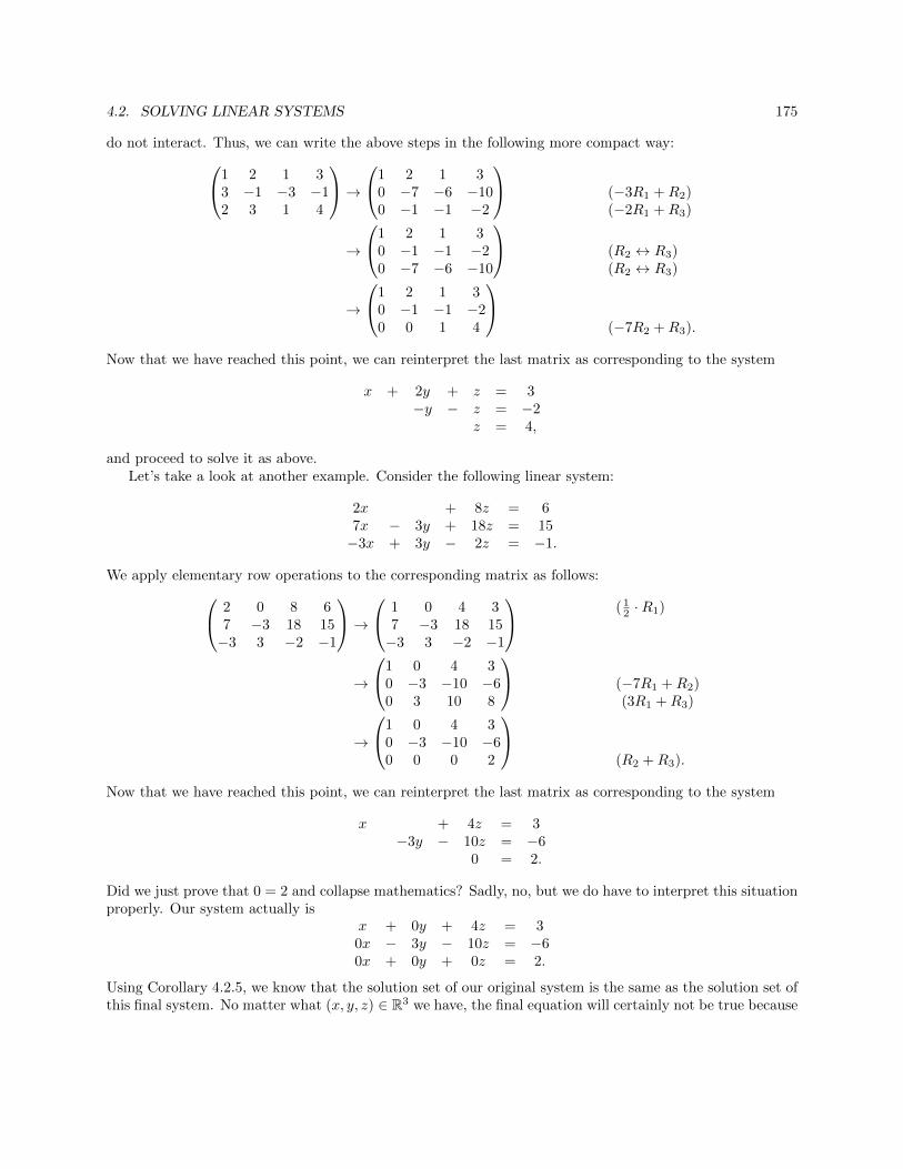
4.2. SOLVING LINEAR SYSTEMS 175
do not interact. Thus, we can write the above steps in the following more compact way:1 2 1 33 −1 −3 −12 3 1 4
→1 2 1 3
0 −7 −6 −100 −1 −1 −2
(−3R1 +R2)(−2R1 +R3)
→
1 2 1 30 −1 −1 −20 −7 −6 −10
(R2 ↔ R3)(R2 ↔ R3)
→
1 2 1 30 −1 −1 −20 0 1 4
(−7R2 +R3).
Now that we have reached this point, we can reinterpret the last matrix as corresponding to the system
x + 2y + z = 3−y − z = −2
z = 4,
and proceed to solve it as above.Let’s take a look at another example. Consider the following linear system:
2x + 8z = 67x − 3y + 18z = 15−3x + 3y − 2z = −1.
We apply elementary row operations to the corresponding matrix as follows: 2 0 8 67 −3 18 15−3 3 −2 −1
→ 1 0 4 3
7 −3 18 15−3 3 −2 −1
( 12 ·R1)
→
1 0 4 30 −3 −10 −60 3 10 8
(−7R1 +R2)(3R1 +R3)
→
1 0 4 30 −3 −10 −60 0 0 2
(R2 +R3).
Now that we have reached this point, we can reinterpret the last matrix as corresponding to the system
x + 4z = 3−3y − 10z = −6
0 = 2.
Did we just prove that 0 = 2 and collapse mathematics? Sadly, no, but we do have to interpret this situationproperly. Our system actually is
x + 0y + 4z = 30x − 3y − 10z = −60x + 0y + 0z = 2.
Using Corollary 4.2.5, we know that the solution set of our original system is the same as the solution set ofthis final system. No matter what (x, y, z) ∈ R3 we have, the final equation will certainly not be true because
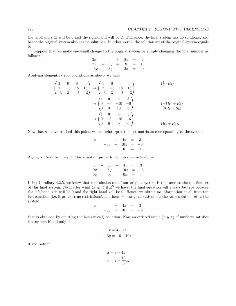
176 CHAPTER 4. BEYOND TWO DIMENSIONS
the left-hand side will be 0 and the right-hand will be 2. Therefore, the final system has no solutions, andhence the original system also has no solutions. In other words, the solution set of the original system equals∅.
Suppose that we make one small change to the original system by simply changing the final number asfollows:
2x + 8z = 67x − 3y + 18z = 15−3x + 3y − 2z = −3.
Applying elementary row operations as above, we have 2 0 8 67 −3 18 15−3 3 −2 −3
→ 1 0 4 3
7 −3 18 15−3 3 −2 −3
( 12 ·R1)
→
1 0 4 30 −3 −10 −60 3 10 6
(−7R1 +R2)(3R1 +R3)
→
1 0 4 30 −3 −10 −60 0 0 0
(R2 +R3).
Now that we have reached this point, we can reinterpret the last matrix as corresponding to the system
x + 4z = 3−3y − 10z = −6
0 = 0.
Again, we have to interpret this situation properly. Our system actually is
x + 0y + 4z = 30x − 3y − 10z = −60x + 0y + 0z = 0.
Using Corollary 4.2.5, we know that the solution set of our original system is the same as the solution setof this final system. No matter what (x, y, z) ∈ R3 we have, the final equation will always be true becausethe left-hand side will be 0 and the right-hand will be 0. Hence, we obtain no information at all from thelast equation (i.e. it provides no restrictions), and hence our original system has the same solution set as thesystem
x + 4z = 3−3y − 10z = −6
that is obtained by omitting the last (trivial) equation. Now an ordered triple (x, y, z) of numbers satisfiesthis system if and only if
x = 3− 4z
−3y = −6 + 10z,
if and only if
x = 3− 4z
y = 2− 10
3z.
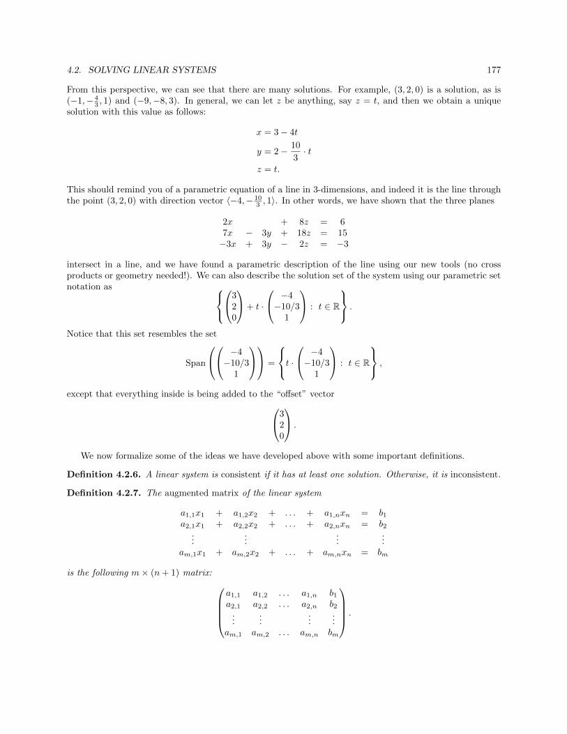
4.2. SOLVING LINEAR SYSTEMS 177
From this perspective, we can see that there are many solutions. For example, (3, 2, 0) is a solution, as is(−1,− 4
3 , 1) and (−9,−8, 3). In general, we can let z be anything, say z = t, and then we obtain a uniquesolution with this value as follows:
x = 3− 4t
y = 2− 10
3· t
z = t.
This should remind you of a parametric equation of a line in 3-dimensions, and indeed it is the line throughthe point (3, 2, 0) with direction vector 〈−4,− 10
3 , 1〉. In other words, we have shown that the three planes
2x + 8z = 67x − 3y + 18z = 15−3x + 3y − 2z = −3
intersect in a line, and we have found a parametric description of the line using our new tools (no crossproducts or geometry needed!). We can also describe the solution set of the system using our parametric setnotation as
320
+ t ·
−4−10/3
1
: t ∈ R
.
Notice that this set resembles the set
Span
−4−10/3
1
=
t · −4−10/3
1
: t ∈ R
,
except that everything inside is being added to the “offset” vector320
.
We now formalize some of the ideas we have developed above with some important definitions.
Definition 4.2.6. A linear system is consistent if it has at least one solution. Otherwise, it is inconsistent.
Definition 4.2.7. The augmented matrix of the linear system
a1,1x1 + a1,2x2 + . . . + a1,nxn = b1a2,1x1 + a2,2x2 + . . . + a2,nxn = b2
......
......
am,1x1 + am,2x2 + . . . + am,nxn = bm
is the following m× (n+ 1) matrix: a1,1 a1,2 . . . a1,n b1a2,1 a2,2 . . . a2,n b2
......
......
am,1 am,2 . . . am,n bm
.
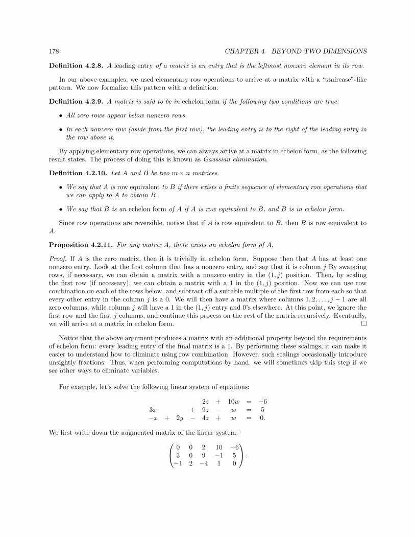
178 CHAPTER 4. BEYOND TWO DIMENSIONS
Definition 4.2.8. A leading entry of a matrix is an entry that is the leftmost nonzero element in its row.
In our above examples, we used elementary row operations to arrive at a matrix with a “staircase”-likepattern. We now formalize this pattern with a definition.
Definition 4.2.9. A matrix is said to be in echelon form if the following two conditions are true:
• All zero rows appear below nonzero rows.
• In each nonzero row (aside from the first row), the leading entry is to the right of the leading entry inthe row above it.
By applying elementary row operations, we can always arrive at a matrix in echelon form, as the followingresult states. The process of doing this is known as Gaussian elimination.
Definition 4.2.10. Let A and B be two m× n matrices.
• We say that A is row equivalent to B if there exists a finite sequence of elementary row operations thatwe can apply to A to obtain B.
• We say that B is an echelon form of A if A is row equivalent to B, and B is in echelon form.
Since row operations are reversible, notice that if A is row equivalent to B, then B is row equivalent toA.
Proposition 4.2.11. For any matrix A, there exists an echelon form of A.
Proof. If A is the zero matrix, then it is trivially in echelon form. Suppose then that A has at least onenonzero entry. Look at the first column that has a nonzero entry, and say that it is column j By swappingrows, if necessary, we can obtain a matrix with a nonzero entry in the (1, j) position. Then, by scalingthe first row (if necessary), we can obtain a matrix with a 1 in the (1, j) position. Now we can use rowcombination on each of the rows below, and subtract off a suitable multiple of the first row from each so thatevery other entry in the column j is a 0. We will then have a matrix where columns 1, 2, . . . , j − 1 are allzero columns, while column j will have a 1 in the (1, j) entry and 0’s elsewhere. At this point, we ignore thefirst row and the first j columns, and continue this process on the rest of the matrix recursively. Eventually,we will arrive at a matrix in echelon form.
Notice that the above argument produces a matrix with an additional property beyond the requirementsof echelon form: every leading entry of the final matrix is a 1. By performing these scalings, it can make iteasier to understand how to eliminate using row combination. However, such scalings occasionally introduceunsightly fractions. Thus, when performing computations by hand, we will sometimes skip this step if wesee other ways to eliminate variables.
For example, let’s solve the following linear system of equations:
2z + 10w = −63x + 9z − w = 5−x + 2y − 4z + w = 0.
We first write down the augmented matrix of the linear system: 0 0 2 10 −63 0 9 −1 5−1 2 −4 1 0
.
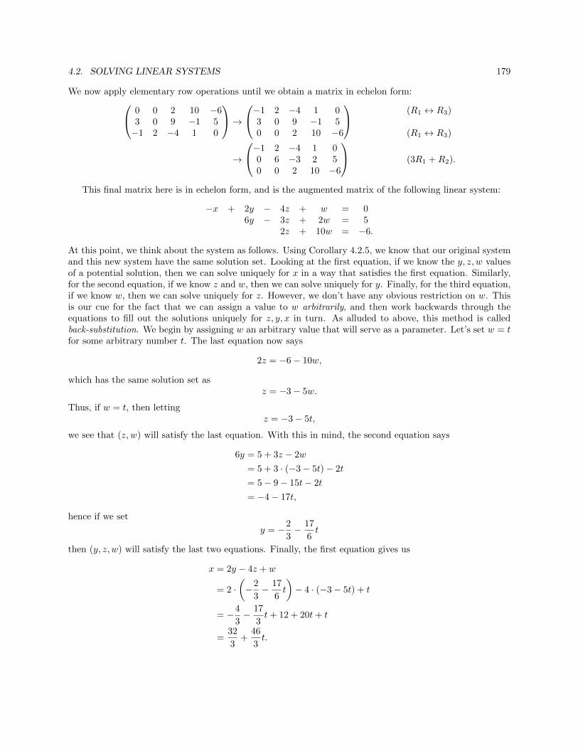
4.2. SOLVING LINEAR SYSTEMS 179
We now apply elementary row operations until we obtain a matrix in echelon form: 0 0 2 10 −63 0 9 −1 5−1 2 −4 1 0
→−1 2 −4 1 0
3 0 9 −1 50 0 2 10 −6
(R1 ↔ R3)
(R1 ↔ R3)
→
−1 2 −4 1 00 6 −3 2 50 0 2 10 −6
(3R1 +R2).
This final matrix here is in echelon form, and is the augmented matrix of the following linear system:
−x + 2y − 4z + w = 06y − 3z + 2w = 5
2z + 10w = −6.
At this point, we think about the system as follows. Using Corollary 4.2.5, we know that our original systemand this new system have the same solution set. Looking at the first equation, if we know the y, z, w valuesof a potential solution, then we can solve uniquely for x in a way that satisfies the first equation. Similarly,for the second equation, if we know z and w, then we can solve uniquely for y. Finally, for the third equation,if we know w, then we can solve uniquely for z. However, we don’t have any obvious restriction on w. Thisis our cue for the fact that we can assign a value to w arbitrarily, and then work backwards through theequations to fill out the solutions uniquely for z, y, x in turn. As alluded to above, this method is calledback-substitution. We begin by assigning w an arbitrary value that will serve as a parameter. Let’s set w = tfor some arbitrary number t. The last equation now says
2z = −6− 10w,
which has the same solution set asz = −3− 5w.
Thus, if w = t, then lettingz = −3− 5t,
we see that (z, w) will satisfy the last equation. With this in mind, the second equation says
6y = 5 + 3z − 2w
= 5 + 3 · (−3− 5t)− 2t
= 5− 9− 15t− 2t
= −4− 17t,
hence if we set
y = −2
3− 17
6t
then (y, z, w) will satisfy the last two equations. Finally, the first equation gives us
x = 2y − 4z + w
= 2 ·(−2
3− 17
6t
)− 4 · (−3− 5t) + t
= −4
3− 17
3t+ 12 + 20t+ t
=32
3+
46
3t.
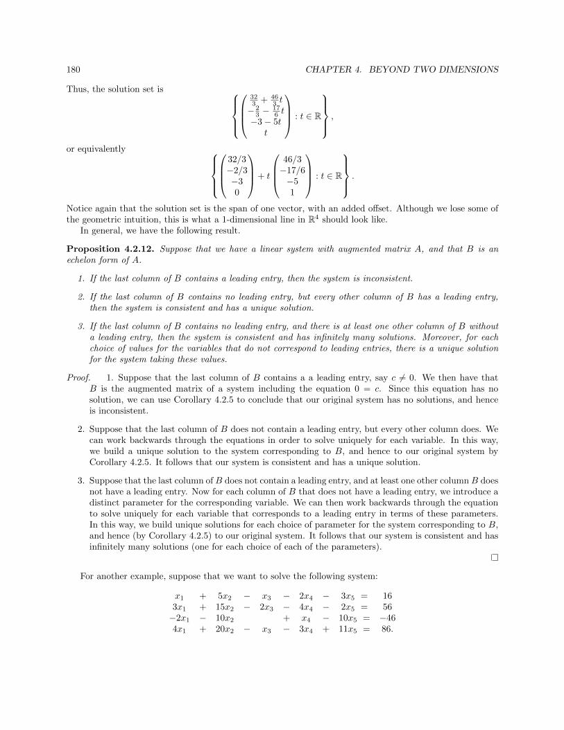
180 CHAPTER 4. BEYOND TWO DIMENSIONS
Thus, the solution set is
323 + 46
3 t− 2
3 −176 t
−3− 5tt
: t ∈ R
,
or equivalently
32/3−2/3−30
+ t
46/3−17/6−51
: t ∈ R
.
Notice again that the solution set is the span of one vector, with an added offset. Although we lose some ofthe geometric intuition, this is what a 1-dimensional line in R4 should look like.
In general, we have the following result.
Proposition 4.2.12. Suppose that we have a linear system with augmented matrix A, and that B is anechelon form of A.
1. If the last column of B contains a leading entry, then the system is inconsistent.
2. If the last column of B contains no leading entry, but every other column of B has a leading entry,then the system is consistent and has a unique solution.
3. If the last column of B contains no leading entry, and there is at least one other column of B withouta leading entry, then the system is consistent and has infinitely many solutions. Moreover, for eachchoice of values for the variables that do not correspond to leading entries, there is a unique solutionfor the system taking these values.
Proof. 1. Suppose that the last column of B contains a a leading entry, say c 6= 0. We then have thatB is the augmented matrix of a system including the equation 0 = c. Since this equation has nosolution, we can use Corollary 4.2.5 to conclude that our original system has no solutions, and henceis inconsistent.
2. Suppose that the last column of B does not contain a leading entry, but every other column does. Wecan work backwards through the equations in order to solve uniquely for each variable. In this way,we build a unique solution to the system corresponding to B, and hence to our original system byCorollary 4.2.5. It follows that our system is consistent and has a unique solution.
3. Suppose that the last column ofB does not contain a leading entry, and at least one other columnB doesnot have a leading entry. Now for each column of B that does not have a leading entry, we introduce adistinct parameter for the corresponding variable. We can then work backwards through the equationto solve uniquely for each variable that corresponds to a leading entry in terms of these parameters.In this way, we build unique solutions for each choice of parameter for the system corresponding to B,and hence (by Corollary 4.2.5) to our original system. It follows that our system is consistent and hasinfinitely many solutions (one for each choice of each of the parameters).
For another example, suppose that we want to solve the following system:
x1 + 5x2 − x3 − 2x4 − 3x5 = 163x1 + 15x2 − 2x3 − 4x4 − 2x5 = 56−2x1 − 10x2 + x4 − 10x5 = −464x1 + 20x2 − x3 − 3x4 + 11x5 = 86.
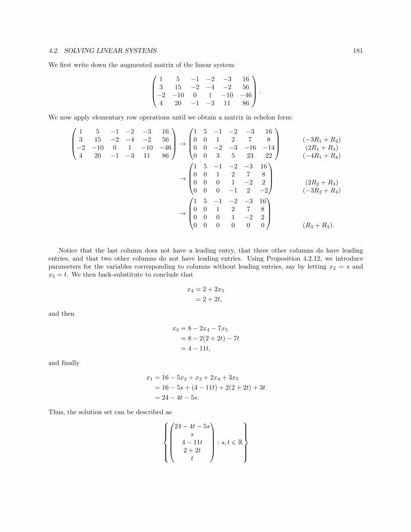
4.2. SOLVING LINEAR SYSTEMS 181
We first write down the augmented matrix of the linear system:1 5 −1 −2 −3 163 15 −2 −4 −2 56−2 −10 0 1 −10 −464 20 −1 −3 11 86
.
We now apply elementary row operations until we obtain a matrix in echelon form:1 5 −1 −2 −3 163 15 −2 −4 −2 56−2 −10 0 1 −10 −464 20 −1 −3 11 86
→
1 5 −1 −2 −3 160 0 1 2 7 80 0 −2 −3 −16 −140 0 3 5 23 22
(−3R1 +R2)(2R1 +R3)
(−4R1 +R4)
→
1 5 −1 −2 −3 160 0 1 2 7 80 0 0 1 −2 20 0 0 −1 2 −2
(2R2 +R3)(−3R2 +R4)
→
1 5 −1 −2 −3 160 0 1 2 7 80 0 0 1 −2 20 0 0 0 0 0
(R3 +R4).
Notice that the last column does not have a leading entry, that three other columns do have leadingentries, and that two other columns do not have leading entries. Using Proposition 4.2.12, we introduceparameters for the variables corresponding to columns without leading entries, say by letting x2 = s andx5 = t. We then back-substitute to conclude that
x4 = 2 + 2x5
= 2 + 2t,
and then
x3 = 8− 2x4 − 7x5
= 8− 2(2 + 2t)− 7t
= 4− 11t,
and finally
x1 = 16− 5x2 + x3 + 2x4 + 3x5
= 16− 5s+ (4− 11t) + 2(2 + 2t) + 3t
= 24− 4t− 5s.
Thus, the solution set can be described as
24− 4t− 5s
s4− 11t2 + 2tt
: s, t ∈ R

182 CHAPTER 4. BEYOND TWO DIMENSIONS
which we can equivalently write as:
240420
+ s
−51000
+ t
−40−11
21
: s, t ∈ R
.
Notice in this case that the solution set can be written as the span of 2 vectors, plus an offset. Geometrically,this feels like a 2-dimensional “plane” in R5, where the offset moves the plane off of the origin. We will discussthese geometric ideas in more detail soon.
By the way, we can continue to perform elementary row operations to simplify the matrix further andavoid back-substitution:
1 5 −1 −2 −3 160 0 1 2 7 80 0 0 1 −2 20 0 0 0 0 0
→
1 5 −1 0 −7 200 0 1 0 11 40 0 0 1 −2 20 0 0 0 0 0
(2R3 +R1)
(−2R3 +R2)
→
1 5 0 0 4 240 0 1 0 11 40 0 0 1 −2 20 0 0 0 0 0
(R2 +R1).
From here, we can obtain the equations we did above with less algebra. Matrices with these additionalproperties are given a special name.
Definition 4.2.13. A matrix is said to be in reduced echelon form if the following conditions are true:
• It is in echelon form.
• The leading entry of every nonzero row is a 1.
• In each column containing a leading entry, all numbers other than this entry are 0.
Although back-substitution from a matrix in echelon will typically be adequate for our current purposes,we will see situations later where it is advantageous to continue on to reduced echelon form.