Embed Size (px)
Citation preview

Linear Algebra II
Course No. 100 222
Spring 2007
Michael Stoll
With some additions by Ronald van Luijk, 2017


Contents
1. Review of Eigenvalues, Eigenvectors and Characteristic Polynomial 22. Direct Sums of Subspaces 33. The Cayley-Hamilton Theorem and the Minimal Polynomial 94. The Structure of Nilpotent Endomorphisms 145. The Jordan Normal Form Theorem 266. The Dual Vector Space 397. Norms on Real Vector Spaces 498. Bilinear Forms 529. Inner Product Spaces 6510. Orthogonal Diagonalization 7711. External Direct Sums 8312. The Tensor Product 8413. Symmetric and Alternating Products 93
Bibliography 101
Index of notation 103
Index 105
1

2 CONTENTS
1. Review of Eigenvalues, Eigenvectors and Characteristic Polynomial
Recall the topics we finished Linear Algebra I with. We were discussing eigenvaluesand eigenvectors of endomorphisms and square matrices, and the question whenthey are diagonalizable. For your convenience, I will repeat here the most relevantdefinitions and results.
Let V be a finite-dimensional F -vector space, dimV = n, and let f : V → V bean endomorphism. Then for λ ∈ F , the λ-eigenspace of f was defined to be
Eλ(f) = {v ∈ V : f(v) = λv} = ker(f − λ idV ) .
λ is an eigenvalue of f if Eλ(f) 6= {0}, i.e., if there is 0 6= v ∈ V such thatf(v) = λv. Such a vector v is called an eigenvector of f for the eigenvalue λ.
The eigenvalues are exactly the roots (in F ) of the characteristic polynomial of f ,
Pf (x) = det(x idV −f) ,
which is a monic polynomial of degree n with coefficients in F .
The geometric multiplicity of λ as an eigenvalue of f is defined to be the dimensionof the λ-eigenspace, whereas the algebraic multiplicity of λ as an eigenvalue of fis defined to be its multiplicity as a root of the characteristic polynomial.
The endomorphism f is said to be diagonalizable if there exists a basis of Vconsisting of eigenvectors of f . The matrix representing f relative to this basis isthen a diagonal matrix, with the various eigenvalues appearing on the diagonal.
Since n× n matrices can be identified with endomorphisms F n → F n, all notionsand results makes sense for square matrices, too. A matrix A ∈ Mat(n, F ) isdiagonalizable if and only if it is similar to a diagonal matrix, i.e., if there is aninvertible matrix P ∈ Mat(n, F ) such that P−1AP is diagonal.
It is an important fact that the geometric multiplicity of an eigenvalue cannotexceed its algebraic multiplicity. An endomorphism or square matrix is diagonal-izable if and only if the sum of the geometric multiplicities of all eigenvalues equalsthe dimension of the space. This in turn is equivalent to the two conditions (a)the characteristic polynomial is a product of linear factors, and (b) for each eigen-value, algebraic and geometric multiplicities agree. For example, both conditionsare satisfied if Pf is the product of n distinct monic linear factors.
Exercises.
(1) Are the vectors
2−1−2
,
−111
, and
4−1−4
linearly independent?
(2) Are the vectors
2−1−2
,
−111
, and
4−1−5
linearly independent?
(3) For which x ∈ R are the vectors
1x0
,
−101
and
11x
linearly depen-
dent?

2. DIRECT SUMS OF SUBSPACES 3
(4) Compute det(M) for
M =
−3 −1 0 −2
0 −2 0 01 0 −1 11 1 0 0
.
(5) Give the kernel and the image of the map R5 → R3 given by x 7→ Axwith
A =
1 −1 1 2 12 −1 4 3 3−1 0 −3 −1 1
.
(6) For any square matrix M show that rk(M2) ≤ rk(M).(7) Compute the characteristic polynomial, the complex eigenvalues and the
complex eigenspaces of the matrix
(0 −11 0
)viewed as a matrix over C.
(8) Find the eigenvalues and eigenspaces of the matrix A =
(11 9−12 −10
).
Is A diagonalizable?
(9) Same question for A =
(3 1−1 1
).
(10) Show that A =
(1 10 1
)is not diagonalizable.
(11) Consider the map f : R2 → R2 given by x 7→ Ax where A =
(3 1−2 0
).
Show that R2 has a basis consisting of eigenvectors of f , and given thematrix of f with respect to this basis. For any positive integer n give aformula for the matrix representation of fn, first with repect to the basisof eigenvectors, and then with repect to the standard basis.
(12) Suppose that M is a diagonalizable matrix. Show that M2 + M is diag-onalizable.
(13) Is every 3×3 matrix whose characteristic polynomial is X3−X diagonal-izable? Is every 3× 3 matrix whose characteristic polynomial is X3−X2
diagonalizable?(14) Let the map f : R3 → R3 be the reflection in the plane x + 2y + z = 0.
What are the eigenvalues and eigenspaces of f?(15) What is the characteristic polynomial of the rotation map R3 → R3 which
rotates space around the line through the origin and the point (1, 2, 3))by 180 degrees? Same question if we rotate by 90 degrees?
2. Direct Sums of Subspaces
The proof of the Jordan Normal Form Theorem, which is one of our goals, uses theidea to split the vector space V into subspaces on which the endomorphism canbe more easily described. In order to make this precise, we introduce the notionof direct sum of linear subspaces of V .
2.1. Definition. Suppose I is an index set and Ui ⊂ V (for i ∈ I) are linearsubspaces of a vector space V satisfying
(1) Uj ∩
∑i∈I\{j}
Ui
= {0}

4 CONTENTS
for all j ∈ I. Then we write⊕
i∈I Ui for the subspace∑
i∈I Ui of V , and we callthis sum the direct sum of the subspaces Ui. Whenever we use this notation, thehypothesis (1) is implied. If I = {1, 2, . . . , n}, then we also write U1⊕U2⊕· · ·⊕Un.
2.2. Lemma. Let V be a vector space, and Ui ⊂ V (for i ∈ I) linear sub-spaces. Then the following statements are equivalent.
(1) Every v ∈ V can be written uniquely as v =∑
i∈I ui with ui ∈ Ui for alli ∈ I (and only finitely many ui 6= 0).
(2)∑
i∈I Ui = V , and for all j ∈ I, we have Uj ∩∑
i∈I\{j} Ui = {0}.(3) If we have any basis Bi of Ui for each i ∈ I, then these bases Bi are
pairwise disjoint, and the union⋃i∈I Bi forms a basis of V.
(4) There exists a basis Bi of Ui for each i ∈ I such that these bases Bi arepairwise disjoint, and the union
⋃i∈I Bi forms a basis of V.
By statement (2) of this lemma, if these conditions are satisfied, then V is thedirect sum of the subspaces Ui, that is, we have V =
⊕i∈I Ui.
Proof. “(1) ⇒ (2)”: Since every v ∈ V can be written as a sum of elementsof the Ui, we have V =
∑i∈I Ui. Now assume that v ∈ Uj ∩
∑i 6=j Ui. This gives
two representations of v as v = uj =∑
i 6=j ui. Since there is only one way ofwriting v as a sum of ui’s, this is only possible when v = 0.
“(2)⇒ (3)”: Since the elements of any basis are nonzero, and Bi is contained in Uifor all i, it follows from Uj ∩
∑i∈I\{j} Ui = {0} that Bi ∩Bj = ∅ for all i 6= j. Let
B =⋃i∈I Bi. Since Bi generates Ui and
∑i Ui = V , we find that B generates V .
To show that B is linearly independent, consider a linear combination∑i∈I
∑b∈Bi
λi,bb = 0 .
For any fixed j ∈ I, we can write this as
Uj 3 uj =∑b∈Bj
λj,bb = −∑i 6=j
∑b∈Bi
λi,bB ∈∑i 6=j
Ui .
By (2), this implies that uj = 0. Since Bj is a basis of Uj, this is only possible whenλj,b = 0 for all b ∈ Bj. Since j ∈ I was arbitrary, this shows that all coefficientsvanish.
“(3) ⇒ (4)”: This follows by choosing any basis Bi for Ui (see Remark 2.3).
“(4) ⇒ (1)”: Take a basis Bi for Ui for each i ∈ I. Write v ∈ V as a linearcombination of the basis elements in
⋃iBi. Since Bi is a basis of Ui, we may write
the part of the linear combination coming from Bi as ui, which yields v =∑
i uiwith ui ∈ Ui. To see that the ui are unique, we note that the ui can be writtenas linear combinations of elements in Bi; the sum v =
∑i ui is then a linear
combination of elements in⋃iBi, which has to be the same as the original linear
combination, because⋃iBi is a basis for V . It follows that indeed all the ui are
uniquely determined. �
2.3. Remark. The proof of the implication (3) ⇒ (4) implicitly assumes theexistence of a basis Bi for each Ui. The existence of a basis Bi for Ui is clearwhen Ui is finite-dimensional, but for infinite-dimensional vector spaces this ismore subtle. Using Zorn’s Lemma, which is equivalent to the Axiom of Choice

2. DIRECT SUMS OF SUBSPACES 5
of Set Theory, one can prove that all vector spaces do indeed have a basis. SeeAppendix D of Linear Algebra I, 2015 edition (or later). We will use this moreoften.
2.4. Remark. If U1 and U2 are linear subspaces of the vector space V, thenstatement V = U1⊕U2 is equivalent to U1 and U2 being complementary subspaces.
2.5. Lemma. Suppose V is a vector space with subspaces U and U ′ such thatV = U⊕U ′. If U1, . . . , Ur are subspaces of U with U = U1⊕· · ·⊕Ur and U ′1, . . . , U
′s
are subspaces of U ′ with U ′ = U ′1 ⊕ · · · ⊕ U ′s, then we have
V = U1 ⊕ · · · ⊕ Ur ⊕ U ′1 ⊕ · · · ⊕ U ′s.
Proof. This follows most easily from part (1) of Lemma 2.2. �
The converse of this lemma is trivial in the sense that if we have
V = U1 ⊕ · · · ⊕ Ur ⊕ U ′1 ⊕ · · · ⊕ U ′s,
then apparently the r + s subspaces U1, . . . , Ur, U′1, . . . , U
′s satisfy the hypothesis
(1), which implies that also the r subspaces U1, . . . , Ur satisfy this hypothesis, aswell as the subspaces U ′1, . . . , U
′s; then also the two subspaces U = U1 ⊕ · · · ⊕ Ur
and U ′ = U ′1 ⊕ . . .⊕ U ′s together satisfy the hypothesis and we have V = U ⊕ U ′.
In other words, we may write
(U1 ⊕ · · · ⊕ Ur)⊕ (U ′1 ⊕ · · · ⊕ U ′s) = U1 ⊕ · · · ⊕ Ur ⊕ U ′1 ⊕ · · · ⊕ U ′sin the sense that if all the implied conditions of the form (1) are satisfied for oneside of the equality, then the same holds for the other side, and the (direct) sumsare then equal. In particular, we have U1 ⊕ (U2 ⊕ · · · ⊕ Ur) = U1 ⊕ · · · ⊕ Ur.
The following lemma states that if two subspaces intersect each other trivially,then one can be extended to a complementary space of the other. Its proof alsosuggests how we can do the extension explicitly.
2.6. Lemma. Let U and U ′ be subspaces of a finite-dimensional vector spaceV satisfying U ∩ U ′ = {0}. Then there exists a subspace W ⊂ V with U ′ ⊂ Wthat is a complementary subspace of U in V .
Proof. Let (u1, . . . , ur) be a basis for U and (v1, . . . , vs) a basis for U ′. ThenLemma 2.2 we have a basis (u1, . . . , ur, v1, . . . , vs) for U + U ′ = U ⊕ U ′. By theBasis Extension Theorem of Linear Algebra 1, we may extend this to a basis(u1, . . . , ur, v1, . . . , vs, w1, . . . , wt) for V . We now let W be the subspace generatedby v1, . . . , vs, w1, . . . , wt. Then (v1, . . . , vs, w1, . . . , wt) is a basis for W and clearlyW contains U ′. By Lemma 2.2 we conclude that U and W are complementaryspaces. �
Next, we discuss the relation between endomorphisms of V and endomorphismsbetween the Ui.

6 CONTENTS
2.7. Lemma and Definition. Let V be a vector space with linear subspacesUi (i ∈ I) such that V =
⊕i∈I Ui. For each i ∈ I, let fi : Ui → Ui be an
endomorphism. Then there is a unique endomorphism f : V → V such thatf |Ui = fi for all i ∈ I.
We call f the direct sum of the fi and write f =⊕
i∈I fi.
Proof. Let v ∈ V . Then we have v =∑
i ui as above, therefore the only wayto define f is by f(v) =
∑i fi(ui). This proves uniqueness. Since the ui in the
representation of v above are unique, f is a well-defined map, and it is clear thatf is linear, so f is an endomorphism of V. �
2.8. Remark. If in the situation of Definition 2.7, V is finite-dimensional andwe choose a basis B of V that is the concatenation of bases Bi of the Ui, thenthe matrix representing f relative to B will be a block diagonal matrix, wherethe diagonal blocks are the matrices representing the fi relative to the bases Bi ofthe Ui. In this finite-dimensional case the number of indices i ∈ I for which Ui isnonzero is finite, and it follows that the characteristic polynomial Pf equals
Pf =∏i∈I
Pfi .
In particular, we have det f =∏
i∈I det fi, and Tr f =∑
i∈I Tr fi for the determi-nant and the trace.
2.9. Remark. An endomorphism f : V → V is diagonalisable if and only ifV is the direct sum of the eigenspaces of f .
2.10. Lemma. Let V be a vector space with linear subspaces Ui (i ∈ I) suchthat V =
⊕i∈I Ui. Let f : V → V be an endomorphism. Then there are endo-
morphims fi : Ui → Ui for i ∈ I such that f =⊕
i∈I fi if and only if each Ui isinvariant under f (or f -invariant), i.e., f(Ui) ⊂ Ui.
Proof. If f =⊕
i fi, then fi = f |Ui , hence f(Ui) = f |Ui(Ui) = fi(Ui) ⊂ Ui.Conversely, suppose that f(Ui) ⊂ Ui. Then we can define fi : Ui → Ui to bethe restriction of f to Ui; it is then clear that fi is an endomorphism of Ui andthat f equals
⊕i fi, as the two coincide on all the subspaces Ui, which together
generate V . �
2.11. Example. Consider the linear map f : R3 → R3 that sends (x, y, z)to (y, z, x). This describes rotation over 2π/3 around the line U1 = L
(a)
witha = (1, 1, 1). The line U1 is point-wise fixed by f , so it is f -invariant. Theorthogonal complement U2 = a⊥ is an f -invariant plane, so we have R3 = U1⊕U2
and f = f1 ⊕ f2 with fi = f |Ui . The vector v1 = a gives a basis for the line U1.The vectors v2 = (1,−1, 0) and v3 = (−1, 0, 1) form a basis (v2, v3) for the planeU2. Putting these two bases together, we obtain a basis B = (v1, v2, v3) for R3 andby the Remark 2.8, the associated matrix [f ]BB is a block diagonal matrix. Indeed,from f(v1) = v1 and f(v2) = v3 and f(v3) = −v2 − v3 we find
[f ]BB =
1 0 00 0 −10 1 −1
.

2. DIRECT SUMS OF SUBSPACES 7
Recall that if V is a vector space over a field F and f : V → V is an endomorphism,then we write
fn = f ◦ f ◦ · · · ◦ f︸ ︷︷ ︸n
.
More generally, if p =∑d
i=0 aixi ∈ F [x] is a polynomial, then we define p(f) =∑d
i=0 aifi. Note that for two polynomials p, q ∈ F [x], we have (p · q)(f) =
p(f) ◦ q(f). We now come to a relation between splittings of f as a directsum and polynomials that vanish on f , that is, polynomials p with p(f) = 0(where 0 denotes the zero endomorphism). We will see later that this includes thecharacteristic and the minimal polynomial of f (see Theorem 3.1 and Lemma 3.4).
We call two polynomials p1(x) and p2(x) coprime if there are polynomials a1(x)and a2(x) such that a1(x)p1(x) + a2(x)p2(x) = 1.
2.12. Lemma. Let V be a vector space and f : V → V an endomorphism.Let p(x) = p1(x)p2(x) be a polynomial such that p(f) = 0 and such that p1(x) andp2(x) are coprime. Let Ui = ker
(pi(f)
), for i = 1, 2. Then V = U1 ⊕ U2 and the
Ui are f -invariant. In particular, f = f1⊕f2, where fi = f |Ui. Moreover, we haveU1 = im
(p2(f)
)and U2 = im
(p1(f)
).
Proof. Set K1 = im(p2(f)
)and K2 = im
(p1(f)
). We first show that Ki ⊂ Ui
for i = 1, 2. Let v ∈ K1 = im(p2(f)
), so v =
(p2(f)
)(u) for some u ∈ V . Then(
p1(f))(v) =
(p1(f)
)((p2(f)
)(u))
=(p1(f)p2(f)
)(u) =
(p(f)
)(u) = 0 ,
so K1 = im(p2(f)
)⊂ ker
(p1(f)
)= U1. The statement for i = 2 follows by
symmetry.
Now we show that U1 ∩ U2 = {0}. So let v ∈ U1 ∩ U2. Then(p1(f)
)(v) =(
p2(f))(v) = 0. Let a1(x), a2(x) be such that a1(x)p1(x) + a2(x)p2(x) = 1. Using
idV = 1(f) =(a1(x)p1(x) + a2(x)p2(x)
)(f) = a1(f) ◦ p1(f) + a2(f) ◦ p2(f) ,
we see that
v =(a1(f)
)((p1(f)
)(v))
+(a2(f)
)((p2(f)
)(v))
=(a1(f)
)(0) +
(a2(f)
)(0) = 0 .
Next, we show that K1 + K2 = V . Using the same relation above, and the factthat pi(f) and ai(f) commute, we find for v ∈ V arbitrary that
v =(p1(f)
)((a1(f)
)(v))
+(p2(f)
)((a2(f)
)(v))∈ im
(p1(f)
)+ im
(p2(f)
).
These statements together imply that Ki = Ui for i = 1, 2, and V = U1 ⊕ U2.Indeed, let v ∈ U1. We can write v = v1 + v2 with vi ∈ Ki. Then U1 3 v − v1 =v2 ∈ U2, but U1 ∩ U2 = {0}, so v = v1 ∈ K1.
Finally, we have to show that U1 and U2 are f -invariant. So let (e.g.) v ∈ U1.Since f commutes with p1(f), we have(p1(f)
)(f(v)
)=(p1(f) ◦ f
)(v) =
(f ◦ p1(f)
)(v) = f
((p1(f)
)(v))
= f(0) = 0 ,
(since v ∈ U1 = ker(p1(f)
)), hence f(v) ∈ U1 as well. �

8 CONTENTS
2.13. Example. Consider the linear map f : R3 → R3 from Example 2.11.Because f 3 = id, we find that the polynomial p = x3−1 vanishes on f , that is, wehave p(f) = 0. We can factor p as p = p1p2 with p1 = x− 1 and p2 = x2 + x+ 1.The polynomials p1 and p2 are coprime, as we have
1 = −13(x+ 2) · p1 + 1
3· p2;
it also follows from Lemma 2.15. We recover U1 and U2 from Example 2.11 asfollows. The linear map p1(f) = f − id sends (x, y, z) to (y−x, z− y, x− z), so wefind ker
(p1(f)
)= L((1, 1, 1)) = U1. The linear map p2(f) = f ◦ f + f + id sends
(x, y, z) to (x+ y + z, x+ y + z, x+ y + z), so we find ker(p1(f)
)= U2.
2.14. Proposition. Let V be a vector space and f : V → V an endomor-phism. Let p(x) = p1(x)p2(x) · · · pk(x) be a polynomial such that p(f) = 0 andsuch that the factors pi(x) are coprime in pairs. Let Ui = ker
(pi(f)
). Then
V = U1 ⊕ · · · ⊕ Uk and the Ui are f -invariant. In particular, f = f1 ⊕ · · · ⊕ fk,where fi = f |Ui.
Proof. We proceed by induction on k. The case k = 1 is trivial. So let k ≥ 2,and denote q(x) = p2(x) · · · pk(x). Then I claim that p1(x) and q(x) are coprime.To see this, note that by assumption, we can write, for i = 2, . . . , k,
ai(x)p1(x) + bi(x)pi(x) = 1 .
Multiplying these equations, we obtain
A(x)p1(x) + b2(x) · · · bk(x)q(x) = 1 ;
note that all the terms except b2(x) · · · bk(x)q(x) that we get when expanding theproduct of the left hand sides contains a factor p1(x).
We can then apply Lemma 2.12 to p(x) = p1(x)q(x) and find that V = U1 ⊕ U ′and f = f1 ⊕ f ′ with U1 = ker
(p1(f)
), f1 = f |U1 , and U ′ = ker
(q(f)
), f ′ = f |U ′ .
In particular, q(f ′) = 0. By induction, we then know that U ′ = U2⊕· · ·⊕Uk withUj = ker
(pj(f
′))
and f ′ = f2⊕· · ·⊕fk, where fj = f ′|Uj , for j = 2, . . . , k. Finally,
ker(pj(f
′))
= ker(pj(f)
)(since the latter is contained in U ′) and fj = f ′|Uj = f |Uj ,
so that we obtain the desired conclusion from Lemma 2.5. �
The following little lemma about polynomials is convenient if we want to applyLemma 2.12.
2.15. Lemma. If p(x) is a polynomial (over F ) and λ ∈ F such that p(λ) 6=0, then (x− λ)m and p(x) are coprime for all m ≥ 1.
Proof. First, consider m = 1. Let
q(x) =p(x)
p(λ)− 1 ;
this is a polynomial such that q(λ) = 0. Therefore, we can write q(x) = (x−λ)r(x)with some polynomial r(x). This gives us
−r(x)(x− λ) +1
p(λ)p(x) = 1 .
Now, taking the mth power on both sides, we obtain an equation(−r(x)
)m(x− λ)m + a(x)p(x) = 1 .
�

3. THE CAYLEY-HAMILTON THEOREM AND THE MINIMAL POLYNOMIAL 9
Exercises. You may use Theorem 3.1 (Cayley-Hamilton) for these exercises.
(1) Let φ : R3 → R3 be a rotation around the line through the origin andthe point (1, 1, 1) by 120 degrees. Decompose R3 as a direct sum of twosubspaces that are each stable under φ.
(2) Consider the vector space V = R3 with the linear map φ : V → V givenby the matrix −1 0 1
−2 −1 1−3 −1 2
Decompose R3 as a direct sum of two subspaces that are each stableunder φ.
(3) Same question for 0 1 15 −4 −3−6 6 5
(4) Consider the vector space V = R4 with the linear map φ : V → V that
permutes the standard basis vectors in a cycle of length 4. What is thecharacteristic polynomial of φ? Decompose R4 into a direct sum of 3subspaces that are all stable under φ.
(5) A nonzero endomorphism f of a vector space V is said to be a projectionif f 2 = f . Suppose f is such a projection.(a) Show that the image of f is equal to the kernel of f − idV , i.e., the
eigenspace E1 at eigenvalue 1.(b) Show that V is the direct sum of the kernel E0 of f and E1.(c) Show that f = f0 ⊕ f1 where f0 is the zero-map on E0 and f1 is the
identity map on E1.(6) An endomorphism f of a vector space V is said to be a reflection if f 2
is the identity on V . Suppose f is such a reflection. Show that V is thedirect sum of two subspaces U and W for which f = idU ⊕(− idW ).
3. The Cayley-Hamilton Theorem and the Minimal Polynomial
Let A ∈ Mat(n, F ). We know that Mat(n, F ) is an F -vector space of dimension n2.
Therefore, the elements I, A,A2, . . . , An2
cannot be linearly independent (becausetheir number exceeds the dimension). If we define p(A) in the obvious way for pa polynomial with coefficients in F (as we already did in the previous chapter),then we can deduce that there is a (non-zero) polynomial p of degree at most n2
such that p(A) = 0 (0 here is the zero matrix). In fact, much more is true.
Consider a diagonal matrix D = diag(λ1, λ2, . . . , λn). (This notation is supposedto mean that λj is the (j, j) entry of D; the off-diagonal entries are zero, of course.)Its characteristic polynomial is
PD(x) = (x− λ1)(x− λ2) · · · (x− λn) .
Since the diagonal entries are roots of PD, we also have PD(D) = 0. More generally,consider a diagonalizable matrix A. Then there is an invertible matrix Q suchthat D = Q−1AQ is diagonal. Since (Exercise!) p(Q−1AQ) = Q−1p(A)Q for p apolynomial, we find
0 = PD(D) = Q−1PD(A)Q = Q−1PA(A)Q =⇒ PA(A) = 0 .
(Recall that PA = PD — similar matrices have the same characteristic polynomial.)

10 CONTENTS
The following theorem states that this is true for all square matrices (or endomor-phisms of finite-dimensional vector spaces).
3.1. Theorem (Cayley-Hamilton). Let A ∈ Mat(n, F ). Then PA(A) = 0.
Proof. Here is a simple, but wrong “proof”. By definition, PA(x) = det(xI−A), so, plugging in A for x, we have PA(A) = det(AI−A) = det(A−A) = det(0) =0. (Exercise: find the mistake!)
For the correct proof, we need to consider matrices whose entries are polynomials.Since polynomials satisfy the field axioms except for the existence of inverses, wecan perform all operations that do not require divisions. This includes addition,multiplication and determinants; in particular, we can use the adjugate matrix.
Let B = xI−A, then det(B) = PA(x). Let B be the adjugate matrix; then we stillhave BB = det(B)I. The entries of B come from determinants of (n−1)× (n−1)submatrices of B, therefore they are polynomials of degree at most n− 1. We canthen write
B = xn−1Bn−1 + xn−2Bn−2 + · · ·+ xB1 +B0 ,
and we have the equality (of matrices with polynomial entries)
(xn−1Bn−1 +xn−2Bn−2 + · · ·+B0)(xI−A) = PA(x)I = (xn+bn−1xn−1 + · · ·+b0)I ,
where we have set PA(x) = xn + bn−1xn−1 + · · ·+ b0. Expanding the left hand side
and comparing coefficients of like powers of x, we find the relations
Bn−1 = I, Bn−2 −Bn−1A = bn−1I, . . . , B0 −B1A = b1I, −B0A = b0I .
We multiply these from the right by An, An−1, . . . , A, I, respectively, and add:
Bn−1An = An
Bn−2An−1 − Bn−1A
n = bn−1An−1
......
...B0A − B1A
2 = b1A− B0A = b0I
0 = PA(A)
�
3.2. Remarks.
(1) The reason why we cannot simply plug in A for x in the identity
B · (xI − A) = PA(x)I
is that whereas x (as a scalar) commutes with the matrices occurring ascoefficients of powers of x, it is not a priori clear that A does so, too.
(2) Another idea of proof (and maybe easier to grasp) is to say that a ‘generic’matrix is diagonalizable (if we assume F to be algebraically closed. . . ),hence the statement holds for ‘most’ matrices. Since it is just a bunch ofpolynomial relations between the matrix entries, it then must hold for allmatrices. This can indeed be turned into a proof, but unfortunately, thisrequires rather advanced tools from algebra.
(3) Of course, the statement of the theorem remains true for endomorphisms.Let f : V → V be an endomorphism of the finite-dimensional F -vectorspace V , then Pf (f) = 0 (which is the zero endomorphism in this case).For evaluating the polynomial at f , we have to interpret fn as the n-foldcomposition f ◦ f ◦ · · · ◦ f , and f 0 = idV .

3. THE CAYLEY-HAMILTON THEOREM AND THE MINIMAL POLYNOMIAL 11
Our next goal is to define the minimal polynomial of a matrix or endomorphism,as the monic polynomial of smallest degree that has the matrix or endomorphismas a “root”. However, we need to know a few more facts about polynomials inorder to see that this definition makes sense.
3.3. Lemma (Polynomial Division). Let f and g be polynomials, with gmonic. Then there are unique polynomials q and r such that r = 0 or deg(r) <deg(g) and such that
f = qg + r .
Proof. We first prove existence, by induction on the degree of f . If deg(f) <deg(g), then we take q = 0 and r = f . So we now assume that m = deg(f) ≥deg(g) = n, f = amx
m+ · · ·+a0. Let f ′ = f −amxm−ng, then (since g = xn+ . . . )deg(f ′) < deg(f). By the induction hypothesis, there are q′ and r such thatdeg(r) < deg(g) or r = 0 and such that f ′ = q′g+r. Then f = (q′+amx
m−n)g+r.(This proof leads to the well-known algorithm for polynomial long division.)
As to uniqueness, suppose we have f = qg + r = q′g + r′, with r and r′ both ofdegree less than deg(g) or zero. Then
(q − q′)g = r′ − r .If q 6= q′, then the degree of the left hand side is at least deg(g), but the degree ofthe right hand side is smaller, hence this is not possible. So q = q′, and thereforer = r′, too. �
Taking g = x− α, this provides a different proof for case k = 1 of Example 8.4 ofLinear Algebra I, 2015 edition (or later).
3.4. Lemma and Definition. Let A ∈ Mat(n, F ). There is a unique monicpolynomial MA of minimal degree such that MA(A) = 0. If p is any polynomialsatisfying p(A) = 0, then p is divisible by MA (as a polynomial).
This polynomial MA is called the minimal (or minimum) polynomial of A. Sim-ilarly, we define the minimal polynomial Mf of an endomorphism f of a finite-dimensional vector space.
Proof. It is clear that monic polynomials p with p(A) = 0 exist (by theCayley-Hamilton Theorem 3.1, we can take p = PA). So there will be such apolynomial of minimal degree. Now assume p and p′ were two such monic polyno-mials of (the same) minimal degree with p(A) = p′(A) = 0. Then we would have(p− p′)(A) = p(A)− p′(A) = 0. If p 6= p′, then we can divide p− p′ by its leadingcoefficient, leading to a monic polynomial q of smaller degree than p and p′ withq(A) = 0, contradicting the minimality of the degree.
Now let p be any polynomial such that p(A) = 0. By Lemma 3.3, there arepolynomials q and r, deg(r) < deg(MA) or r = 0, such that p = qMA + r.Plugging in A, we find that
0 = p(A) = q(A)MA(A) + r(A) = q(A) · 0 + r(A) = r(A) .
If r 6= 0, then deg(r) < deg(MA), but the degree of MA is the minimal possibledegree for a polynomial that vanishes on A, so we have a contradiction. Thereforer = 0 and hence p = qMA. �

12 CONTENTS
3.5. Remark. In Introductory Algebra, you will learn that the set of polyno-mials as discussed in the lemma forms an ideal and that the polynomial ring is aprincipal ideal domain, which means that every ideal consists of the multiples ofsome fixed polynomial. The proof is exactly the same as for the lemma.
By Lemma 3.4, the minimal polynomial divides the characteristic polynomial. Asa simple example, consider the identity matrix In. Its characteristic polynomial is(x− 1)n, whereas its minimal polynomial is x− 1. In some sense, this is typical,as the following result shows.
3.6. Proposition. Let A ∈ Mat(n, F ) and λ ∈ F . If λ is a root of thecharacteristic polynomial of A, then it is also a root of the minimal polynomialof A. In other words, both polynomials have the same linear factors.
Proof. If PA(λ) = 0, then λ is an eigenvalue of A, so there is 0 6= v ∈ F n
such that Av = λv. Setting MA(x) = amxm + · · ·+ a0, we find
0 = MA(A)v =m∑j=0
ajAjv =
m∑j=0
ajλjv = MA(λ)v .
(Note that the terms in this chain of equalities are vectors.) Since v 6= 0, thisimplies MA(λ) = 0.
By Lemma 3.4, we know that each root of MA is a root of PA, and we have justshown the converse. So both polynomials have the same linear factors. �
3.7. Remark. If F is algebraically closed (i.e., every non-zero polynomial isa product of linear factors), this shows that PA is a multiple of MA, and Mk
A isa multiple of PA when k is large enough. In fact, the latter statement is true forgeneral fields F (and can be interpreted as saying that both polynomials have thesame irreducible factors). For the proof, one replaces F by a larger field F ′ suchthat both polynomials split into linear factors over F ′. That this can always bedone is shown in Introductory Algebra.
One nice property of the minimal polynomial is that it provides another criterionfor diagonalizability.
3.8. Proposition. Let A ∈ Mat(n, F ). Then A is diagonalizable if and onlyif its minimal polynomial MA is a product of distinct monic linear factors.
Proof. First assume that A is diagonalizable. It is easy to see that similarmatrices have the same minimal polynomial (Exercise), so we can as well assumethat A is already diagonal. But for a diagonal matrix, the minimal polynomialis just the product of factors x − λ, where λ runs through the distinct diagonalentries. (It is the monic polynomial of smallest degree that has all diagonal entriesas roots.)
Conversely, assume that MA(x) = (x − λ1) · · · (x − λm) with λ1, . . . , λm ∈ Fdistinct. The polynomials qi = x − λi (with 1 ≤ i ≤ m) are pairwise coprime, soby Proposition 2.14 the eigenspaces
Ui = Eλi(A) = ker(A− λiI) = ker qi(A)
satisfy F n = U1 ⊕ · · · ⊕ Um. This implies n =∑m
i=1 dimEλi(A), which in turn(by Cor. 11.24 of Linear Algebra I, 2015 edition) implies that A is diagonalizable.
�

3. THE CAYLEY-HAMILTON THEOREM AND THE MINIMAL POLYNOMIAL 13
3.9. Example. Consider the matrix
A =
1 1 10 1 10 0 1
.
Is it diagonalizable?
Its characteristic polynomial is clearly PA(x) = (x−1)3, so its minimal polynomialmust be (x− 1)m for some m ≤ 3. Since A− I 6= 0, m > 1 (in fact, m = 3), henceA is not diagonalizable.
On the other hand, the matrix (for F = R, say)
B =
1 2 30 4 50 0 6
has MB(x) = PB(x) = (x− 1)(x− 4)(x− 6); therefore, B is diagonalizable.
Exercise: what happens for fields F of small characteristic?
3.10. Corollary. Let f : V → V be a diagonalisable endomorphism of afinite-dimensional vector space V . Let U ⊂ V be an f -invariant subspace. Thenthe restriction f |U is also diagonalisable.
Proof. By Proposition 3.8, the minimal polynomial Mf of f is the productof distinct linear factors. The endomorphism Mf (f |U) is the restriction to U ofMf (f) = 0, so the minimal polynomial of f |U divides Mf by Lemma 3.4, and istherefore also the product of distinct linear factors. Proposition 3.8 then impliesthat f |U is diagonalisable. �
Exercises.
(1) What is the remainder when one divides the polynomial x5 +x by x2 +1?(2) Give the minimal polynomial and the characteristic polynomial of the
matrices 2 −3 33 −4 33 −3 2
,
0 −1 31 −2 33 −3 2
.
(3) Suppose that a 2×2 matrix A has two distinct eigenvalues λ and µ. Showthat the image of the matrix A− λ is the eigenspace with eigenvalue µ.
(4) Is the matrix
0 0 −31 0 00 1 0
diagonalizable over R? And over C?
(5) If f : R3 → R3 is the projection on a plane, what is the minimum poly-nomial of f? What is the minimum polynomial of relection in a plane?
(6) Compute the characteristic polynomial of the matrix
A =
1 −9 41 −4 11 −7 3
.
Compute A3 (use Cayley-Hamilton!)(7) Let V be the 4 dimensional vector space of polynomial functions R→ R of
degree at most 3. Let T : V → V be the map that sends a polynomial p toits derivative T (p) = p′. Show that T is a linear map. Is T diagonalizable?

14 CONTENTS
(8) For each α ∈ R, determine the characteristic and minimal polynomials of
Aα =
1− α α 02− α α− 1 α
0 0 −1
.
For which values of α is Aα diagonalizable?(9) Let M be a square matrix satisfying M3 = M . What can you say about
the eigenvalues of M? Show that M is diagonalizable.
4. The Structure of Nilpotent Endomorphisms
4.1. Definition. A matrix A ∈ Mat(n, F ) is said to be nilpotent, if Am = 0for some m ≥ 1. Similarly, if V is a finite-dimensional vector space and f : V → Vis an endomorphism, then f is said to be nilpotent if fm = f ◦ f ◦ · · · ◦ f︸ ︷︷ ︸
m times
= 0 for
some m ≥ 1.
It follows that the minimal polynomial of A or f is of the form xm, where m isthe smallest number that has the property required in the definition.
4.2. Proposition. A nilpotent matrix or endomorphism is diagonalizable ifand only if it is zero.
Proof. The minimal polynomial is xm. Prop. 3.6 then implies that the matrixor endomorphism is diagonalizable if and only if m = 1. But then the minimalpolynomial is x, which means that the matrix or endomorphism is zero. �
Theorem 4.7 tells us more about the structure of nilpotent endomorphisms. It isthe main ingredient to proving the existence of the Jordan Normal Form. We firststate some lemmas that will be useful for the proof of Theorem 4.7.
4.3. Lemma. Let V be a vector space and f : V → V an endomorphism.Suppose m > 0 is an integer such that fm = 0. If for each j ∈ {0, 1, . . . ,m − 1}we have a complementary subspace Xj of ker f j inside ker f j+1, then we have
V = X0 ⊕X1 ⊕X2 ⊕ . . .⊕Xm−1.
Proof. Note that we have ker fm = V and ker f 0 = {0}. For all j ∈{0, 1, . . . ,m− 1}, we have ker f j+1 = ker f j ⊕Xj, so we find
V = ker fm = ker fm−1 ⊕Xm−1 = (ker fm−2 ⊕Xm−2)⊕Xm−1 =
= ker fm−2 ⊕Xm−2 ⊕Xm−1 = · · · = ker f 0 ⊕X0 ⊕X1 ⊕ . . .⊕Xm−1 =
= X0 ⊕X1 ⊕ . . .⊕Xm−1.
�

4. THE STRUCTURE OF NILPOTENT ENDOMORPHISMS 15
4.4. Lemma. Let f : V → W be a linear map of vector spaces, and X ⊂ Vand Y ⊂ W subspaces such that X ∩ f−1(Y ) = {0}. Then f restricts to aninjective map X ↪→ W , and we have f(X) ∩ Y = {0}.
Proof. The kernel of the restriction f = f |X : X → W satisfies
ker f = X ∩ ker f ⊂ X ∩ f−1(Y ) = {0},so f is injective. The last part of the statement follows from the fact that, moregenerally, the restriction X∩f−1(Y )→ f(X)∩Y of f is surjective (the verificationof this fact is left as an exercise for the reader). �
4.5. Lemma. Let V be a vector space and f : V → V an endomorphism. Letj ≥ 1 be an integer. If X is a complementary space of ker f j inside ker f j+1, thenf restricts to an injective map X ↪→ ker f j and we have f(X) ∩ ker f j−1 = {0}.
Proof. Note that for every i ≥ 0, we have f−1(ker f i) = ker f i+1. For i = j,this implies that f restricts to a linear map f ′ : ker f j+1 → ker f j. For i = j − 1and Y = ker f j−1, it implies f−1(Y ) = ker f j, so we get
X ∩ f ′−1(Y ) ⊂ X ∩ f−1(Y ) = {0}.Hence, the statement follows directly from Lemma 4.4, applied to f ′, X, and Y .
�
4.6. Remark. In terms of quotient spaces, Lemma 4.4 can be phrased by say-ing that f induces an injective map V/f−1(Y )→ W/Y , which follows from one ofthe isomorphism theorems (analogous to those from group theory), applied to thelinear map V → W/Y with kernel f−1(Y ). Similarly, Lemma 4.5 can be phrasedby saying that f induces an injective map ker f j+1/ ker f j ↪→ ker f j/ ker f j−1.
4.7. Theorem. Let V be an F -vector space, dimV = n, and let f : V → Vbe a nilpotent endomorphism. Then V has a basis (v1, v2, . . . , vn) such that f(vj)is either zero or vj+1.
Proof. Let m be a positive integer such that fm = 0. In each of m steps,numbered j = m,m − 1, . . . , 2, 1, we will construct an integer tj and vectorswj1, . . . , wjtj ∈ ker f j such that the elements
(2)(fk−j(wkl)
)j≤k≤m1≤l≤tk
form a basis for a complementary space Xj−1 of ker f j−1 inside ker f j. For j = m,we take any basis (wm1, . . . , wmtm) for a complementary subspace of ker fm−1 insideker fm = V . Assume 1 ≤ j < m and suppose that we have already constructedintegers and vectors as above in all steps m,m− 1, . . . , j + 1. Then the elements
(3)(fk−(j+1)(wkl)
)j+1≤k≤m1≤l≤tk
form a basis for a complementary space Xj of ker f j inside ker f j+1. The map frestricts to an injective map Xj → ker f j by Lemma 4.5. This implies that theimages
(4)(fk−j(wkl)
)j+1≤k≤m1≤l≤tk
of the elements in (3) form a basis for the subspace f(Xj) ⊂ ker f j (see Lemma 7.13of Linear Algebra I, 2015 edition (or later) for linear independence), which againby Lemma 4.5 satisfies f(Xj) ∩ ker f j−1 = {0}. By Lemma 2.6 we can extend
16 CONTENTS
the basis (4) for f(Xj) to a basis for a complementary subspace Xj−1 of ker f j−1
inside ker f j; we denote the added basis vectors by wj1, wj2, . . . , wjtj . Adding theseelements to (4) gives (2), with the new elements corresponding to k = j.
By Lemma 4.3, we have V = X0 ⊕ X1 ⊕ X2 ⊕ . . . ⊕ Xm−1, so the bases (2) forthe Xj are disjoint and their union forms a basis for V (see Lemma 2.2). Writingi = k − j, this union consists of the elements
(5)(f i(wkl)
)1≤k≤m1≤l≤tk0≤i<k
.
Note that for any indices 1 ≤ k ≤ m and 1 ≤ l ≤ tk, we have wkl ∈ ker fk, sof(fk−1(wkl)) = 0. Hence, if we order the elements of (5) lexicographically by theirindex triples (k, l, i), then we obtain a basis as mentioned in the theorem. �
Although the following proof is called an alternative proof, it is essentially the sameas the proof above, but it has Lemmas 4.3 and 4.5 incorporated. The subspace Ujfrom this proof is the subpace Xj ⊕Xj+1 ⊕ · · · ⊕Xm from the proof above.
Alternative proof. Let m be an integer such that fm = 0. Note that wehave a chain of inclusions
{0} = ker f 0 ⊂ ker f 1 ⊂ ker f 2 ⊂ · · · ⊂ ker fm−1 ⊂ ker fm = V.
We prove by descending induction that for all j ∈ {0, 1, . . . ,m} there are elementsw1, . . . , ws ∈ V and non-negative integers e1, . . . , es, such that the sequence
(6)(w1, f(w1), . . . , f
e1(w1), w2, f(w2), . . . , fe2(w2), . . . , ws, f(ws), . . . , f
es(ws))
is a basis of a complementary space Uj of ker f j inside V and the elementsf e1+1(w1), . . . , f
es+1(ws) are contained in ker f j.
For j = m we have ker fm = V , so we may take s = 0 and Um = {0}. Suppose0 ≤ j < m and suppose that we have elements w1, . . . , wr ∈ V and integersd1, . . . , dr, such that the sequence analogous to (6), with r instead of s and withdi instead of ei, is a basis for a complementary subspace Uj+1 of ker f j+1 inside V ,and the elements fd1+1(w1), . . . , f
dr+1(wr) are contained in ker f j+1.
We claim that if any scalars λ1, . . . , λr satisfy∑r
i=1 λifdi+1(wi) ∈ ker f j, then we
have λ1 = · · · = λr = 0. Indeed, set z =∑r
i=1 λifei(wi). Then the assumption
states that f(z) ∈ ker f j, so we have z ∈ ker f j+1. But z is also a linear combi-nation of elements in a basis for Uj+1, so we have z ∈ Uj+1 ∩ ker f j+1 = {0} andthus z = 0, which in turn implies λ1 = · · · = λr = 0. This proves the claim.
The claim implies in particular that the elements fdi+1(wi) for i = 1, . . . , r arelinearly independent, so they form a basis for the subspace Wj ⊂ ker f j+1 thatthey generate. The claim also implies Wj ∩ ker f j = {0}, so Wj can be extendedto a complementary space Xj of ker f j inside ker f j+1, and the basis for Wj canbe extended to a basis (fd1+1(w1), . . . , f
dr+1(wr), wr+1, . . . , ws) for Xj. Set Uj =Uj+1 ⊕Xj. Then we have
V = Uj+1 ⊕ ker f j+1 = Uj+1 ⊕ (Xj ⊕ ker f j) = (Uj+1 ⊕Xj)⊕ ker f j = Uj ⊕ ker f j,
so Uj is a complementary space of ker f j in V . The union of the two bases forUj+1 and Xj gives a basis for Uj. If we set ei = di + 1 for 1 ≤ i ≤ r and ei = 0for r < i ≤ s, then we can rearrange this basis to (6), which finishes the inductionstep.

4. THE STRUCTURE OF NILPOTENT ENDOMORPHISMS 17
The statement of the Theorem now follows from the case j = 0, as the onlycomplementary subspace of ker f 0 = {0} is V , and we may denote the elements of(6) for j = 0 by v1, v2, . . . , vn. �
4.8. Remark. If (v1, . . . , vn) is a basis as in Theorem 4.7, then the matrixA = (aij) representing f with respect to (vn, . . . , v2, v1), has all entries zero exceptaj,j+1 = 1 if f(vn−j) = vn+1−j. Therefore A is a block diagonal matrix
A =
B1 0 · · · 0
0 B2 · · · 0...
.... . .
...
0 0 · · · Bk
where for each i there is an integer m ≥ 1 such that the i-th block Bi is the m×mblock
B(m) =
0 1 0 · · · 00 0 1 · · · 0...
......
. . ....
0 0 0 · · · 10 0 0 · · · 0
with all zeroes except for ones just above the diagonal. Note that we reversedthe order of the basis elements! Also note that B(m)m = 0, and for each integer1 ≤ s < m, the matrix B(m)s is the m×m matrix with all zeroes, except for oneson the diagonal that is s positions above the main diagonal.
4.9. Corollary. Every nilpotent matrix is similar to a matrix of the form justdescribed.
Proof. This is clear from our discussion. �
4.10. Corollary. A matrix A ∈ Mat(n, F ) is nilpotent if and only if its char-acteristic polynomial is PA(x) = xn.
Proof. If PA(x) = xn, then An = 0 by the Cayley-Hamilton Theorem 3.1,hence A is nilpotent. Conversely, if A is nilpotent, then it is similar to a matrixof the form above, which visibly has characteristic polynomial xn. �
4.11. Remark. The statement of Cor. 4.10 would also follow from the factthat PA(x) divides some power of MA(x) = xm, see Remark 3.7. However, wehave proved this only in the case that PA(x) splits into linear factors (which weknow is true, but only after the fact).
4.12. Remark. The proof of Theorem 4.7 gives an efficient algorithm to con-struct such a special basis. In terms of the alternative proof, we can state it asfollows.
(1) Compute an m with fm = 0.(2) Start with j = m and Xm = {0} and tm = 0 and the empty basis for Xm.(3) Decrease j by 1.

18 CONTENTS
• We now have a basis(f e1(w1), f
e2(w2), . . . , fes(ws)
)for a complement Xj+1 of ker f j+1 in ker f j+2.
(4) Extend f e1+1(w1), . . . , fes+1(ws) to a basis
f e1+1(w1), . . . , fes+1(ws), ws+1, . . . , wt
of a complementary space Xj of ker f j in ker f j+1 (see Lemma 2.6).(5a) For 1 ≤ i ≤ s, increase ei by 1.(5b) For s < i ≤ t, set ei = 0.(5c) Set s equal to t.(6a) If j > 0, go back to (3).(6b) If j = 0, then we are done: the union of the bases of X0, . . . , Xm−1 can
be reordered to give a basis for V as in Theorem 4.7.
4.13. Example. Consider
A =
3 4 −71 2 −32 3 −5
∈ Mat(3,R) .
We find
A2 =
−1 −1 2−1 −1 2−1 −1 2
and A3 = 0, so A is nilpotent. Let us find a basis as given in Theorem 4.7.The first step in the process comes down to finding a complementary subspaceof ker(A2) = L
((2, 0, 1)>, (−1, 1, 0)>
). We can take (1, 0, 0)>, for example, as the
basis of a complement. This will be w1 in the notation of the proof above. Wethen have Aw1 = (3, 1, 2)> and A2w1 = (−1,−1,−1)>, and these three alreadyform a basis. Reversing the order, we get−1 3 1
−1 1 0−1 2 0
−13 4 −71 2 −32 3 −5
−1 3 1−1 1 0−1 2 0
=
0 1 00 0 10 0 0
.
The following proposition tells us how many blocks of each size to expect.
4.14. Proposition. Let f : V → V be a nilpotent endomorphism of a finite-dimensional vector space V . Let B = (vn, . . . , v1) be a basis for V such that itsreverse is a basis as in Theorem 4.7. Let A = [f ]BB be the associated matrix. Forevery integer j ≥ 0 we set rj = dim ker f j, and for every integer j ≥ 1 we setsj = rj − rj−1 and tj = sj − sj+1. Then for every integer j ≥ 1 there are exactly tjblocks of the form B(j) of size j × j along the diagonal of A.
Proof. The matrix A is described in Remark 4.8. Let m1,m2, . . . ,mk ≥ 0 beintegers such that the blocks along the diagonal of A are B(m1), . . . , B(mk). Foreach integer j ≥ 0, the matrix Aj is a block matrix with blocks B(m1)
j, . . . , B(mk)j
along the diagonal. Therefore, the matrixAj is in row echelon form, and for every i,the first min(mi, j) columns corresponding to the i-th block B(mi)
j do not containa pivot, while the other columns do contain pivots. Hence, the kernel of Aj hasdimension
rj =k∑i=1
min(mi, j)
4. THE STRUCTURE OF NILPOTENT ENDOMORPHISMS 19
and we find
sj = rj − rj−1 =k∑i=1
(min(mi, j)−min(mi, j − 1)
).
As for integers a, b the value min(a, b) − min(a, b − 1) equals 0 for a < b and itequals 1 otherwise, we conclude that sj equals the number of blocks of size atleast j. Therefore, the number of blocks of size exactly j is sj − sj+1 = tj. �
4.15. Remark. The tk from the proof of Theorem 4.7 are the same as thetk from the proof of Proposition 4.14. Indeed, for fixed integers 1 ≤ k ≤ m and1 ≤ l ≤ tk, with tk as in the proof of Theorem 4.7, the k elements f i(wkl) with0 ≤ i < k in (5) correspond to a block of size k × k, so there are tk such blocks.Moreover, with rk and sk as in Proposition 4.14, the proof of Theorem 4.7 shows
dimXk−1 = dim ker fk − dim ker fk−1 = rk − rk−1 = sk.
This also implies for tk as defined in the proof of Theorem 4.7 that we have
tk = dimXk−1 − dim f(Xk) = dimXk−1 − dimXk = sk − sk+1.
While this seems to give another proof of Proposition 4.14, this argument a priorionly holds for bases that are obtained as in the proof of Theorem 4.7. It is howevernot hard to show that every basis as mentioned in Theorem 4.7 can indeed beobtained through the construction in the proof of Theorem 4.7, so it does yield asecond proof.
4.16. Example. In Example 4.13, we have rkA = 2 and rkA2 = 1 andA3 = 0, so we get the following table.
j rj sj tj0 01 1 1 02 2 1 03 3 1 14 3 0 05 3 0
We conclude, as we have seen in the example above, that there is an invertiblematrix Q such that Q−1AQ consists of one block B(3).
4.17. Corollary. Let A,A′ ∈ Mat(n, F ) be two nilpotent matrices. Then Aand A′ are similar if and only if for each integer 1 ≤ j < n we have dim kerAj =dim kerA′j.
Proof. For every integer j ≥ 0, and every square matrix M , set rj(M) =kerM j. For j ≥ 1, also set sj(M) = rj(M) − rj−1(M) and tj(M) = sj(M) −sj+1(M). Of course, if A and A′ are similar, then rj(A) = rj(A
′) for each j.Conversely, suppose that for each integer 1 ≤ j < n we have rj(A) = rj(A
′). ByCayley-Hamilton, we have An = A′n = 0, so for j ≥ n we have rj(A) = rj(A
′) aswell, as both equal n. For j = 0 both equal 0, so we have rj(A) = rj(A
′) for allj ≥ 0. This implies that for all j ≥ 1 we have sj(A) = sj(A
′) and tj(A) = tj(A′),
so by Proposition 4.14, both A and A′ are similar to a block diagonal matrix withtj(A) = tj(A
′) blocks of the form B(j) along the diagonal for every j ≥ 1. Anytwo such matrices are similar to each other; in fact they can be obtained fromeach other by a permutation of the basis. By transitivity of similarity, also A andA′ are similar. �

20 CONTENTS
4.18. Example. Consider the real matrix
A =
−5 10 −8 4 1−4 8 −10 8 2−3 6 −12 12 3−2 4 −8 4 10−1 2 −4 2 5
.
We compute
A2 =
0 0 0 −18 360 0 0 −36 720 0 0 −54 1080 0 0 −36 720 0 0 −18 36
and A3 =
0 0 0 0 00 0 0 0 00 0 0 0 00 0 0 0 00 0 0 0 0
,
so we can start the algorithm of Remark 4.12 with m = 3. The kernel kerA isgenerated by
x = (−3, 0, 3, 2, 1) and x′ = (2, 1, 0, 0, 0).
(We urge the reader to verify this, either by bringing A into row echelon formby elementary row operations, or by verifying that A has rank 3, concludingthat kerA has dimension 2, and checking that x and x′ are linearly independentelements contained in kerA.) The kernel kerA2 is generated by
e1 = (1, 0, 0, 0, 0), e2 = (0, 1, 0, 0, 0), e3 = (0, 0, 1, 0, 0), and y = (0, 0, 0, 2, 1).
Clearly, we have kerA3 = R5. In terms of Proposition 4.14, with rj = dim kerAj,we find r0 = 0 and r1 = 2 and r2 = 4 and rn = 5 for n ≥ 3; this yields s1 = 2 ands2 = 2 and s3 = 1 and s4 = 0. Finally, we obtain t1 = 0 and t2 = 1 and t3 = 1,so we already find that the standard nilpotent form consists of one block of size 2and one block of size 3.
To find an appropriate basis, we start with picking a complementary space X2
of kerA2 inside kerA3 = R5. Since dim kerA3 − dim kerA2 = 3 − 2 = 1, itsuffices to pick any element of R5 that is not contained in kerA2. We choose w1 =e5 = (0, 0, 0, 0, 1), which gives Aw1 = (1, 2, 3, 10, 5) and A2w1 = 36(1, 2, 3, 2, 1)en A3w1 = 0. This gives X2 = 〈w1〉. In the next step, we are looking for acomplementary space X1 of kerA inside kerA2 such that f(X2) ⊂ X1. In otherwords, we want to extend f(X2) = 〈Aw1〉 to a complementary space of kerA insidekerA2. In order to do this, we follow the proof of Lemma 2.6 in the book: take abasis for kerA and for f(X2) and put the elements of these two bases as columnsin a matrix; we also take generators for kerA2 and add these as columns to thematrix. We obtain
−3 2 1 1 0 0 00 1 2 0 1 0 03 0 3 0 0 1 02 0 10 0 0 0 21 0 5 0 0 0 1
.
A row echelon form for this matrix is1 0 5 0 0 0 10 1 2 0 1 0 00 0 12 0 0 −1 30 0 0 1 −2 1 00 0 0 0 0 0 0
,

4. THE STRUCTURE OF NILPOTENT ENDOMORPHISMS 21
which has pivots in the first three columns as expected. Of the last four columns,only the first contains a pivot, so in order to extend f(X2) to a complementaryspace X1 as mentioned, it suffices to add the first generator for kerA2, so we takew2 = (1, 0, 0, 0, 0), which gives Aw2 = −(5, 4, 3, 2, 1). The last step, namely findinga complementary space X0 for kerA0 = {0} inside kerA which contains f(X1), istrivial, as f(X1) is generated by A2w1 and Aw2, so dim f(X1) = 2 = dim kerA,so we have X0 = f(X1) and we do not need to extend.
Hence, we obtain a basis B = (A2w1, Aw1, w1, Aw2, w2) (note the order of theelements). If we denote the standard basis for R5 by E, the basis transformationmatrix
P = [id]BE =
36 1 0 −5 172 2 0 −4 0108 3 0 −3 072 10 0 −2 036 5 1 −1 0
satisfies
P−1AP =
0 1 0 0 00 0 1 0 00 0 0 0 00 0 0 0 10 0 0 0 0
.
4.19. Example. From small examples one does not always get a good ideaof the general case, so we now do a bigger example. If the reader wishes to verifythe calculations, we recommend using a computer.
Let M be the 11× 11 real matrix
M =
14 15 0 8 −40 32 −2 −72 −8 0 −20−29 −34 −7 −16 55 −64 14 137 16 0 31
6 10 2 4 −18 15 −2 −33 −5 0 −10−3 −2 2 −1 −10 0 −2 3 0 1 −6−6 −7 0 −4 24 −15 −1 34 4 0 1214 7 −4 6 −28 24 5 −56 −4 0 −12−3 −4 −1 −2 9 −8 2 17 2 0 510 7 −2 5 −26 20 2 −46 −4 0 −12−67 −77 −14 −38 130 −148 30 319 36 1 72−53 −54 −2 −28 102 −108 10 241 26 1 5212 15 2 8 −42 30 −1 −66 −8 0 −22
.
One checks that M4 = 0, so M is nilpotent.
Moreover, one checks that M , M2, and M3 have rank 7, 4, and 1, respectively.This gives the following table.
j rj sj tj0 01 4 4 12 7 3 03 10 3 24 11 1 15 11 0 06 11 0

22 CONTENTS
We conclude that there is an invertible matrix Q such that QMQ−1 is a blockmatrix consisting of one block B(1), two blocks B(3), and one block B(4) alongits diagonal.
To find such a matrix Q, we will construct a basis (v1, v2, . . . , v11) as in Theo-rem 4.7. As in the proof of that theorem, we note that Mm = 0 for m = 4, sowe start with j = m − 1 = 3 (having trivially taken care of j = m). We want topick a basis for a complementary space U3 of kerM3 inside kerM4 = R11; giventhat we have dim kerM3 = 10, we find dimU3 = 1, so it suffices to find a vectorv1 ∈ R11 that is not contained in kerM3. The 3-rd, 7-th, and 10-th column ofM3 are the only zero columns, so the standard basis vector ej is not containedin kerM3 for j 6∈ {3, 7, 10}. Because the fourth column of M3 contains relativelysmall numbers, we choose v1 = e4, and define vj = Mvj−1 for 2 ≤ j ≤ 4. Thisgives
v1 =
00010000000
, v2 =
8−16
4−1−46−25−38−28
8
, v3 =
4−730−20−11−15−11
4
, v4 =
1−20−20201−5−60
.
These vectors correspond to a block of the form B(4). To check consistency, onecould verify that indeed we have Mv4 = 0. Note that Mv3 = v4, so M2v3 = 0,which implies v3 ∈ kerM2 \ kerM . Similarly, we have Mv2 = v3, from which weconclude v2 ∈ kerM3 \ kerM2.
We continue with j = 2. We want to pick a basis for some complementary spaceU2 of kerM2 inside kerM3 that contains v2 (this is the only vector of the fourthat we already found that is contained in kerM3 but not in kerM2). This willrequire some computation and then we use Lemma 2.6. One computes that thekernel kerM2 is generated by the columns of the matrix
K2 =
1 0 0 0 0 0 00 1 0 0 0 0 00 0 1 0 0 0 00 0 0 1 0 0 00 0 0 0 1 0 00 0 0 0 0 1 02 3 0 0 0 0 44 5 −1 0 −1 0 7−32 −41 9 1 9 4 −61−7 −7 1 1 1 0 −11−1 −1 0 0 −2 0 −1
.

4. THE STRUCTURE OF NILPOTENT ENDOMORPHISMS 23
Moreover, the kernel kerM3 is generated by the columns of the matrix
K3 =
1 0 0 0 0 0 0 0 0 00 1 0 0 0 0 0 0 0 00 0 1 0 0 0 0 0 0 00 0 0 1 0 0 0 0 0 00 0 0 0 1 0 0 0 0 00 0 0 0 0 1 0 0 0 00 0 0 0 0 0 1 0 0 00 0 0 0 0 0 0 1 0 00 0 0 1 0 0 0 1 2 00 0 0 0 0 0 0 0 0 11 1 0 0 −2 2 0 −5 −1 0
Lemma 2.6 tells us that in order to extend v2 to a basis of a complementary spaceof kerM2 inside kerM3, we take the columns of K2 together with v2, and extendthis to a basis of kerM3 by adding some of the columns of K3. We do this bytaking the extended matrix
(K1|v2|K2)
and using elementary row operations to bring this into (reduced) row echelon form.This yields
1 0 0 0 0 0 0 0 0 0 −18 7 −18 −4 24 −15 2 −70 1 0 0 0 0 0 0 0 3 36 −12 36 8 −50 28 −4 120 0 1 0 0 0 0 0 0 2 −7 4 −8 0 10 −12 0 −40 0 0 1 0 0 0 0 0 2 3 1 3 2 −5 −2 −1 00 0 0 0 1 0 0 0 0 3 10 −2 11 4 −15 2 −2 20 0 0 0 0 1 0 0 0 3 −12 6 −12 1 15 −18 0 −60 0 0 0 0 0 1 0 0 0 −16 6 −16 −2 22 −17 1 −60 0 0 0 0 0 0 1 0 2 3 0 3 2 −5 −2 −1 00 0 0 0 0 0 0 0 1 4 2 1 2 4 −4 −9 −2 −10 0 0 0 0 0 0 0 0 5 2 2 2 4 −5 −10 −2 −20 0 0 0 0 0 0 0 0 0 0 0 0 0 0 0 0 0
.
Since the first two columns of the right part of this matrix are the ones that containa pivot, we see that we may add the corresponding first two columns of K3 to v2to obtain a complementary space of kerM2 inside kerM3. The first two columnsof K3 are e1 + e11 and e1 + e11, so we find
U2 = L(v2, e1 + e11, e2 + e11
).
Note, as a consistency check, that indeed we have dimU2+dim kerM2 = dim kerM3,that is, 3 + 7 = 10. Write v5 = e1 + e11 and v6 = Mv5 and v7 = Mv6, as well asv8 = e2 + e11, and v9 = Mv8 and v10 = Mv9. Then we have v7, v10 ∈ kerM . Thevectors v5, v6, v7 correspond to a block of the form B(3), and so do v8, v9, v10.
We proceed with j = 1. We want to pick a basis for some complementary spaceU1 of kerM inside kerM2 that contains v3, v6, v9 (these are the only vectors of theten that we found so far that are contained in kerM2 but not in kerM). FromdimU1 = kerM2 − dim kerM = 7− 4 = 3, we find that the linearly independentvectors v3, v6, and v9 already span U1. This corresponds to the fact that there areno blocks of the form B(2), as we had already seen.
Finally, for j = 0, we want to pick a basis for some complementary space U0
of kerM0 = ker I11 = {0} inside kerM that contains v4, v7, v10 (these are thevectors among those that we found so far that are contained in kerM but not in

24 CONTENTS
kerM0 = {0}). We do this by writing down an extended matrix with v4, v7, v10 ascolumns on the left, and four generators for kerM on the right, say
1 −2 −1 1 0 0 0−2 4 2 2 4 0 00 −1 1 0 0 1 0−2 4 2 −4 −2 0 00 2 3 0 0 0 12 −6 −10 0 −2 −2 −20 0 0 0 0 0 01 −3 −5 0 −1 −1 −1−5 11 9 4 9 1 1−6 13 10 −3 3 1 10 −4 −6 −1 −1 0 −2
.
The associated reduced row echelon form is
1 0 2 0 −1 0 10 1 4 0 0 1 10 0 5 0 0 2 10 0 0 1 1 0 00 0 0 0 0 0 00 0 0 0 0 0 00 0 0 0 0 0 00 0 0 0 0 0 00 0 0 0 0 0 00 0 0 0 0 0 00 0 0 0 0 0 0
.
Since the first column on the right is the only column on the right with a pivot,we add only the first of the four chosen generators for kerM , so
v11 =
120−400004−3−1
.
We conclude that (v1, v2, . . . , v11) is a basis as in Theorem 4.7. Putting the elevenvectors in reverse order, we obtain the basis B = (v11, . . . , v2, v1). If we let E

4. THE STRUCTURE OF NILPOTENT ENDOMORPHISMS 25
denote the standard basis, and we set
Q = [id]BE =
1 −1 −5 0 −2 −6 1 1 4 8 02 2 −3 1 4 2 0 −2 −7 −16 00 1 0 0 −1 −4 0 0 3 4 0−4 2 −8 0 4 −9 0 −2 0 −1 10 3 5 0 2 6 0 0 −2 −4 00 −10 −5 0 −6 2 0 2 0 6 00 0 1 0 0 2 0 0 −1 −2 00 −5 −5 0 −3 −2 0 1 1 5 04 9 −5 0 11 5 0 −5 −15 −38 0−3 10 −2 0 13 −1 0 −6 −11 −28 0−1 −6 −7 1 −4 −10 1 0 4 8 0
,
then we find
Q−1MQ = [id]EB[fM ]EE[id]BE = [fM ]BB =
0 0 0 0 0 0 0 0 0 0 00 0 1 0 0 0 0 0 0 0 00 0 0 1 0 0 0 0 0 0 00 0 0 0 0 0 0 0 0 0 00 0 0 0 0 1 0 0 0 0 00 0 0 0 0 0 1 0 0 0 00 0 0 0 0 0 0 0 0 0 00 0 0 0 0 0 0 0 1 0 00 0 0 0 0 0 0 0 0 1 00 0 0 0 0 0 0 0 0 0 10 0 0 0 0 0 0 0 0 0 0
.
Exercises.
(1) Let A be a nilpotent n× n matrix. Show that idn +A is invertible.(2) Let A be a nilpotent n× n matrix. Show that An = 0.(3) Let N be a 9× 9 matrix for which N3 = 0. Suppose that N2 has rank 3.
Prove that N has rank 6.(4) Let N be a 12× 12 matrix for which N4 = 0.
(a) Show that the kernel of N2 contains the image of N2.(b) Show that the rank of N is at most 9.(c) Show that the rank of N is equal to 9 if the kernel of N2 is equal to
the image of N2.(5) For which x ∈ R is the following matrix nilpotent? 2x x −1
−4 −1 −35 2 3
(6) For each of the matrices 4 −4 12
1 −1 3−1 1 −3
2 0 80 1 1−1 1 −3
give a basis of R3 for which the matrix sends each basis vector either to0 or to the next basis vector in the basis.

26 CONTENTS
(7) Do the same for the matrix1 1 0 0−5 −2 2 −1−3 0 2 −1−5 −2 2 −1
5. The Jordan Normal Form Theorem
In this section, we will formulate and prove the Jordan Normal Form Theorem,which will tell us that any matrix whose characteristic polynomial is a product oflinear factors is similar to a matrix of a very special near-diagonal form.
Now we can feed this into Prop. 2.14.
5.1. Theorem. Let V be a finite-dimensional vector space, and let f : V → Vbe an endomorphism whose characteristic polynomial splits into linear factors:
Pf (x) = (x− λ1)m1 · · · (x− λk)mk ,where the λi are distinct. Then for the generalized λi-eigenspaces
Ui = ker(f − λi idV )mi
of f we have V = U1⊕· · ·⊕Uk and f = f |U1⊕· · ·⊕f |Uk . Moreover, dimUi = mi,and for all k ≥ mi we have ker(f − λi idV )k = Ui.
Proof. Write Pf (x) = p1(x) · · · pk(x) with pi(x) = (x−λi)mi . By the Cayley-Hamilton Theorem 3.1, we know that Pf (f) = 0. By Lemma 2.15, we know thatthe pi(x) are coprime in pairs. The first result then follows from Prop. 2.14. Setfi = f |Ui . For the dimension of Ui, we note that the characteristic polynomial Pfiof fi is a divisor of Pf that only has λi as eigenvalue, as fi−λi idUi is nilpotent. ByRemark 2.8, we have Pf =
∏i Pfi , so we conclude Pfi = (x− λi)mi , which implies
dimUi = mi. Finally, as the map (f − λi idV )mi kills Ui, its image is the same asits image on
⊕j 6=i Uj. By Lemma 2.12 this image is
⊕j 6=i Uj itself, so the map is
an isomorphism on⊕
j 6=i Uj, and hence so is f − λi idV as well as any power of it.
Since (f −λi idV )k for k ≥ mi also kills Ui, this implies that (f −λi idV )k also hasthe same image, and thus the same rank and nullity (dimension of the kernel) as(f − λi idV )mi . Hence, the inclusion Ui ⊂ ker(f − λi idV )k is an equality. �
5.2. Theorem (Jordan Normal Form). Let V be a finite-dimensional vec-tor space, and let f : V → V be an endomorphism whose characteristic polynomialsplits into linear factors:
Pf (x) = (x− λ1)m1 · · · (x− λk)mk ,where the λi are distinct. Then there is a basis of V such that the matrix repre-senting f with respect to that basis is a block diagonal matrix with blocks of theform
B(λ,m) =
λ 1 0 · · · 0 00 λ 1 · · · 0 00 0 λ · · · 0 0...
......
. . ....
...0 0 0 · · · λ 10 0 0 · · · 0 λ
∈ Mat(F,m)
where λ ∈ {λ1, . . . , λk}.

5. THE JORDAN NORMAL FORM THEOREM 27
Proof. We keep the notations of Theorem 5.1. We know that on Ui, (f −λi id)mi = 0, so f |Ui = λi idUi + gi, where gmii = 0, i.e., gi is nilpotent. ByTheorem 4.7, there is a basis of Ui such that gi is represented by a block diagonalmatrix Bi with blocks of the form B(0,m) (such that the sum of the m’s is mi).Therefore, f |Ui is represented by Bi + λiIdimUi , which is a block diagonal matrixcomposed of blocks B(λi,m) (with the same m’s as before). The basis of V that isthe concatenation of the various bases of the Ui then does what we want, compareRemark 2.8. �
We say that a matrix is in Jordan normal form if it is a diagonal block matrixwith all blocks along the diagonal of the form B(λ,m) for some λ ∈ F and someinteger m ≥ 0.
5.3. Remark. Let V , f , and λ1, . . . , λk ∈ F be as in Theorem 5.2. Let B bea basis as is claimed to exist, and let A = [f ]BB be the matrix associated to f withrespect to B. Take any element λ ∈ F . For every integer i ≥ 0 we set rj(λ) =dim ker(f − λ idV )j, and for every integer j ≥ 1 we set sj(λ) = rj(λ) − rj−1(λ)and tj(λ) = sj(λ)− sj+1(λ). Then for every integer j ≥ 1 there are exactly tj(λ)blocks of the form B(λ, j) along the diagonal of A.
Indeed, for λ not a root of the characteristic polynomial Pf , we get rj(λ) =sj(λ) = tj(λ) = 0 for all j, and no blocks of the form B(λ, j) for any j. If λ = λifor some i, then in terms of the notation of the proof of Theorem 5.2, we can applyProposition 4.14 to the nilpotent endomorphisn gi = f |Ui − λ idUi , which satisfiesgmii = 0. Note that for every integer j ≥ 0 the kernel ker(f − λi idV )j is contained
in ker(f − λi idV )mi = Ui by Theorem 5.1. Hence this kernel equals ker gji , and we
find rj(λi) = dim ker gji . Proposition 4.14 the states that there are tj(λi) blocks ofthe form B(0, j) in a diagonal block matrix for gi, and these blocks correspond toblocks in A of the form B(λi, j).
5.4. Corollary. Let A,A′ ∈ Mat(n, F ) be two square matrices such that thecharacteristic polynomial of A splits into linear factors, that is,
PA(x) = (x− λ1)m1 · · · (x− λk)mk .Then A and A′ are similar if and only if for each index 1 ≤ i ≤ k and each integer1 ≤ j ≤ mi we have dim ker(A− λiI)j = dim ker(A′ − λiI)j.
Proof. If A and A′ are similar, then the claimed equality of dimensions holds.For the converse, assume that for every index 1 ≤ i ≤ k and for each integer1 ≤ j ≤ mi we have dim ker(A − λiI)j = dim ker(A′ − λiI)j. Then in particular,this holds for j = mi. Since ker(A−λi)mi is the generalised eigenspace associatedto λi for A, we find that for each i, the dimension of the generalised eigenspaceassociated to λi is at least as large for A′ as for A. Since the sum of the dimensionsof all generalised eigenspaces for A and for A′ are both equal to n, we find thatequality holds for each i, and furthermore, A′ has no other eigenvalues. It followsthat the characteristic polynomials of A and A′ are the same. From Remark 5.3we conclude that A and A′ are both similar to a block diagonal matrices B and B′,respectively, where B and B′ have the same blocks along the diagonal. For details,compare to the proof of Corollary 4.17. Then B and B′ are similar, as they canbe obtained from each other by a permutation of the basis. So by transitivity ofsimilarity, also A and A′ are similar. �
Here is a less precise, but for many applications sufficient version of Theorem 5.2.

28 CONTENTS
5.5. Corollary. Let V be a finite-dimensional vector space, and let f : V →V be an endomorphism whose characteristic polynomial splits into linear factors,as above. Then we can write f = d + n, with endomorphisms d and n of V, suchthat d is diagonalizable, n is nilpotent, and d and n commute: d ◦ n = n ◦ d.
Proof. We just take d to be the endomorphism corresponding to the ‘diagonalpart’ of the matrix given in Theorem 5.2 and n to be that corresponding to the‘nilpotent part’ (obtained by setting all diagonal entries equal to zero). Since thetwo parts commute within each ‘Jordan block,’ the two endomorphisms commute.
�
5.6. Example. Let us compute the Jordan Normal Form and a suitable basisfor the endomorphism f : R3 → R3 given by the matrix
A =
0 1 00 0 1−4 0 3
.
We first compute the characteristic polynomial:
Pf (x) =
∣∣∣∣∣∣x −1 00 x −14 0 x− 3
∣∣∣∣∣∣ = x2(x− 3) + 4 = x3 − 3x2 + 4 = (x− 2)2(x+ 1) .
We see that it splits into linear factors, which is good. We now have to find thegeneralized eigenspaces. We have a simple eigenvalue −1; the eigenspace is
E−1(f) = ker
1 1 00 1 1−4 0 4
= L((1,−1, 1)>
),
so for a basis we can choose w1 = (1,−1, 1)>. The other eigenspace is
E2(f) = ker
−2 1 00 −2 1−4 0 1
= L((1, 2, 4)>
).
This space has only dimension 1, so f is not diagonalizable, and we have to lookat the generalized eigenspace:
ker((f − 2 id)2
)= ker
4 −4 1−4 4 −14 −4 1
= L((1, 1, 0)>, (1, 0,−4)>
).
As a basis for this generalised eigenspace, we start with a basis for a complementaryspace of ker(f−2 id) inside ker(f−2 id)2. Such a complementary space has dimen-sion dim ker(f − 2 id)2−dim ker(f − 2 id) = 2− 1 = 1, so we can take any elementin ker(f−2 id)2 that is not contained in ker(f−2 id), say w2 = (1, 1, 0)>. As basisfor this generalised eigenspace, we then obtain w2, (f−2 id)(w2) = (−1,−2,−4)>.Reversing the order we get a basis for R3 consisting of the elements
(−1,−2,−4)>, (1, 1, 0)>, (1,−1, 1)> ,
and we find−1 1 1−2 1 −1−4 0 1
−1 0 1 00 0 1−4 0 3
−1 1 1−2 1 −1−4 0 1
=
2 1 00 2 00 0 −1
.

5. THE JORDAN NORMAL FORM THEOREM 29
As mentioned in Example 4.19, from small examples one does not always get anidea of the general case, so at the end of this chapter, we will do some biggerexamples.
5.7. Application. One important application of the Jordan Normal FormTheorem is to the explicit solution of systems of linear first-order differential equa-tions with constant coefficients. Such a system can be written
d
dty(t) = A · y(t) ,
where y is a vector-valued function and A is a matrix. One can then show (Exer-cise) that there is a unique solution with y(0) = y0 for any specified initial value y0,and it is given by
y(t) = exp(tA) · y0with the matrix exponential
exp(tA) =∞∑n=0
tn
n!An .
If A is in Jordan Normal Form, the exponental can be easily determined. Ingeneral, A can be transformed into Jordan Normal Form, the exponential can beevaluated for the transformed matrix, then we can transform it back — note that
exp(tP−1AP ) = P−1 exp(tA)P .
5.8. Remark. Writing an endomorphism f : V → V as f = n + d with ddiagonalisable and n nilpotent and d ◦ n = n ◦ d is very useful for computingpowers of f , as for every positive integer k, we have
fk =k∑i=0
(k
i
)dk−ini,
and if nm = 0 for some integer m, then all terms with i ≥ m vanish.
5.9. Remark. What can we do when the characteristic polynomial does notsplit into linear factors (which is possible when the field F is not algebraicallyclosed)? In this case, we have to use a weaker notion than that of diagonalizability.Define the endomorphism f : V → V to be semi-simple if every f -invariantsubspace U ⊂ V has an f -invariant complementary subspace in V . One can show(exercise) that if the characteristic polynomial of f splits into linear factors, thenf is semi-simple if and only if it is diagonalizable. The general version of theJordan Normal Form Theorem then is as follows.
Let V be a finite-dimensional vector space, f : V → V an endomorphism. Thenf = s + n with endomorphisms s and n of V such that s is semi-simple, n isnilpotent, and s ◦ n = n ◦ s.
Unfortunately, we do not have the means and time to prove this result here.
However, we can state the result we get over F = R.

30 CONTENTS
5.10. Theorem (Real Jordan Normal Form). Let V be a finite-dimensionalreal vector space, f : V → V an endomorphism. Then there is a basis of V suchthat the matrix representing f with respect to this basis is a block diagonal matrixwith blocks of the form B(λ,m) and of the form (with µ > 0)
B′(λ, µ,m) =
λ −µ 1 0 · · · 0 0 0 0µ λ 0 1 · · · 0 0 0 00 0 λ −µ · · · 0 0 0 00 0 µ λ · · · 0 0 0 0...
......
.... . .
......
......
0 0 0 0 · · · λ −µ 1 00 0 0 0 · · · µ λ 0 10 0 0 0 · · · 0 0 λ −µ0 0 0 0 · · · 0 0 µ λ
∈ Mat(R, 2m) .
Blocks B(λ,m) occur for eigenvalues λ of f ; blocks B′(λ, µ,m) occur if Pf (x) isdivisible by x2 − 2λx+ λ2 + µ2.
Proof. Here is a sketch that gives the main ideas. First choose any basisB = (x1, . . . , xn) for V , so that ϕB : Rn → V given by (λ1, . . . , λn) 7→
∑i λixi
is an isomorphism. Identifying V with Rn through this isomorphism reduces theproblem to the case V = Rn, which is naturally contained in Cn, and f : Rn → Rn
being given by a real n× n matrix A.
Over C, the characteristic polynomial Pf = PA will split into linear factors. Someof them will be of the form x − λ with λ ∈ R, the others will be of the formx− (λ+ µi) with λ, µ ∈ R and µ 6= 0. These latter ones occur in pairs
(x− (λ+ µi))(x− (λ− µi)) = x2 − 2λx+ λ2 + µ2 .
If v1, . . . , vm ∈ Cn is a basis of the generalized eigenspace (over C) for the eigen-value λ+µi, then v1, . . . , vm is a basis of the generalized eigenspace for the eigen-value λ− µi, where v denotes the vector obtained from v ∈ Cn by replacing eachcoordinate with its complex conjugate. If we now consider
(v1 + v1), i(v1 − v1), . . . , (vm + vm), i(vm − vm) ,
then these vectors are in Rn and form a basis of the sum of the two generalizedeigenspaces. If (v1, . . . , vm) gives rise to a Jordan block B(λ+µi,m), then we have
f(vi + vi) = f(vi) + f(vi) = f(vi) + f(vi)
= (λ+ µi)vi + v′i−1 + (λ− µi)vi + v′i−1
= λ(vi + vi) + µi(vi − vi) + v′i−1 + v′i−1,
f(i(vi − vi)) = if(vi)− if(vi) = i · f(vi)− i · f(vi)
= i(λ+ µi)vi + iv′i−1 − i(λ− µi)vi − iv′i−1= λi(vi − vi)− µ(vi + vi) + i(v′i−1 − v′i−1),
for v′i−1 = 0 if i = 1 and v′i−1 = vi−1 if i > 1, so the new basis gives rise to a blockof the form B′(λ, µ,m). �

5. THE JORDAN NORMAL FORM THEOREM 31
5.11. Theorem. Let V be a finite-dimensional vector space, f1, . . . , fk : V →V diagonalizable endomorphisms that commute in pairs. Then f1, . . . , fk are si-multaneously diagonalizable, i.e., there is a basis of V consisting of vectors thatare eigenvectors for all the fj at the same time. In particular, any linear combi-nation of the fj is again diagonalizable.
Proof. First note that if f and g are commuting endomorphisms and v is aλ-eigenvector of f , then g(v) is again a λ-eigenvector of f (or zero):
f(g(v)
)= g(f(v)
)= g(λv) = λg(v) .
We now proceed by induction on k. For k = 1, there is nothing to prove. So assumek ≥ 2. We can write V = U1⊕· · ·⊕Ul, where the Ui are the nontrivial eigenspacesof fk. By the observation just made, we have splittings, for j = 1, . . . , k − 1,
fj = f(1)j ⊕ · · · ⊕ f
(l)j with f
(i)j : Ui → Ui.
By Corollary 3.10, the restrictions f(i)j : Ui → Ui are diagonalisable, so by the
induction hypothesis, f(i)1 , . . . , f
(i)k−1 are simultaneously diagonalizable on Ui, for
each i. Since Ui consists of eigenvectors of fk, any basis of Ui that consists ofeigenvectors of all the fj, j < k, will also consist of eigenvectors for all the fj,j ≤ k. To get a suitable basis of V , we take the union of the bases of thevarious Ui. �
To finish this section, here is a uniqueness statement related to Cor. 5.5.
5.12. Theorem. The diagonalizable and nilpotent parts of f in Cor. 5.5 areuniquely determined.
Proof. Let f = d + n = d′ + n′, where d and n are constructed as in theJordan Normal Form Theorem 5.2 and d ◦ n = n ◦ d, and d′ ◦ n′ = n′ ◦ d′. Thend′ and n′ commute with f (d′ ◦ f = d′ ◦ d′ + d′ ◦ n′ = d′ ◦ d′ + n′ ◦ d′ = f ◦ d′,same for n′). Now let g be any endomorphism commuting with f , and considerv ∈ Uj = ker((f − λj id)mj). Then
(f − λj id)mj(g(v)
)= g((f − λj id)mj(v)
)= g(0) = 0 ,
so g(v) ∈ Uj, i.e., Uj is g-invariant. So g = g1 ⊕ · · · ⊕ gk splits as a direct sumof endomorphisms of the generalized eigenspaces Uj of f . Since on Uj, we havef |Uj = λj id +n|Uj and g commutes with f , we find that gj commutes with n|Ujfor all j, hence g commutes with n (and also with d).
Applying this to d′ and n′, we see that d and d′ commute, and that n and n′
commute. We can write
d− d′ = n′ − n ;
then the right hand side is nilpotent (for this we need that n and n′ commute!).By Theorem 5.11, the left hand side is diagonalizable, so we can assume it isrepresented by a diagonal matrix. But the only nilpotent diagonal matrix is thezero matrix, therefore d− d′ = n′ − n = 0, i.e., d′ = d and n′ = n. �
As promised, we will now give some bigger examples of matrices that we will putin Jordan normal form.

32 CONTENTS
5.13. Example. Consider the matrix
A =
2 3 3 3 30 −1 0 −1 −10 0 −1 1 00 0 0 −1 10 0 0 0 −1
.
We want an invertible matrix Q and a matrix J in Jordan normal form suchthat A = QJQ−1. The characteristic polynomial of A is (x − 2)(x + 1)4, so theeigenvalues are 2 and −1. The dimensions of the generalised eigenspaces equal thealgebraic multiplicities, so they equal 1 and 4, respectively.
The dimension of the eigenspace associated to an eigenvalue is at least 1, so forthe eigenvalue λ = 2 the associated eigenspace ker(A − 2I) is the whole gener-alised eigenspace, as both have dimension 1. The element e1 is contained in theeigenspace, so w0 = e1 generates this subspace.
For the eigenvalue λ = −1, we have
A+ I =
3 3 3 3 30 0 0 −1 −10 0 0 1 00 0 0 0 10 0 0 0 0
, (A+ I)2 =
9 9 9 9 90 0 0 0 −10 0 0 0 10 0 0 0 00 0 0 0 0
and
(A+ I)3 =
27 27 27 27 270 0 0 0 00 0 0 0 00 0 0 0 00 0 0 0 0
.
Because (A+I)3 has rank 1 we have dim ker(A+I)3 = 5−1 = 4. As the generalisedeigenspace has dimension 4, the subspace U = ker(A+I)3 is the whole generalisedeigenspace. The kernels ker(A + I)n for n = 1, 2, 3 are easy to determine, since(A+ I)n is already in row echelon form. We find
ker(A+ I) = L((−1, 1, 0, 0, 0), (−1, 0, 1, 0, 0)
),
ker(A+ I)2 = L((−1, 1, 0, 0, 0), (−1, 0, 1, 0, 0), (−1, 0, 0, 1, 0)
),
ker(A+ I)3 = L((−1, 1, 0, 0, 0), (−1, 0, 1, 0, 0), (−1, 0, 0, 1, 0), (−1, 0, 0, 0, 1)
).
Hence, for the dimension rj(−1) = dim(A+I)n we have r1(−1) = 2 and r2(−1) = 3and r3(−1) = 4. We get s1(−1) = 2 and s2(−1) = 1 and s3(−1) = 1. We also gett1(−1) = 1 and t2(−1) = 0 and t3(−1) = 1, so there are two Jordan blocks, oneof size 1× 1 and one of size 3× 3.
For the largest block, we choose a complementary subspace of ker(A + I)2 insideker(A + I)3; this complementary space has dimension r3 − r2 = 1, so it sufficesto pick on vector: a vector in ker(A + I)3 \ ker(A + I)2, so for example w1 =(−1, 0, 0, 0, 1). The other two vectors associated to the 3×3 block are (A+I)w1 =(0,−1, 0, 1, 0) and (A+ I)2w1 = (0,−1, 1, 0, 0).
A complementary subspace for ker(A + I) inside ker(A + I)2 also has dimensionr2−r1 = 1 and it is therefore generated by (A+ I)w1. A complementary subspacefor ker(A+I)0 = {0} inside ker(A+I) is equal to ker(A+I), which has dimension2; we already have a vector, namely (A + I)2w1 = (0,−1, 1, 0, 0), so in order to

5. THE JORDAN NORMAL FORM THEOREM 33
generate ker(A + I), it suffices to add a vector from ker(A + I) that is not amultiple of (A + I)2w1. For example, we may choose w2 = (−1, 1, 0, 0, 0). Thisvector corresponds to the 1× 1 blok.
The vectors w0, (A+I)2w1, (A+I)w1, w1, w2 form a basis B. If we put the vectorsin this order in a matrix, then we get
Q = [id]BE =
1 0 0 −1 −10 −1 −1 0 10 1 0 0 00 0 1 0 00 0 0 1 0
,
where E d is the standard basis. The associated Jordan normal for is then
J = [fA]BB =
2 0 0 0 00 −1 1 0 00 0 −1 1 00 0 0 −1 00 0 0 0 −1
.
Indeed, one verifies QJQ−1 = [id]BE · [fA]BB · [id]EB = [fA]EE = A.
5.14. Example. We consider the real matrix
M =
−1 1 −1 1 −1 1 −1 1 −1 10 −1 3 −3 3 −3 3 −3 3 −30 0 2 0 1 −1 1 −1 1 −10 0 0 2 1 −1 1 −1 1 −10 0 0 0 2 0 1 −1 1 −10 0 0 0 0 2 1 −1 1 −10 0 0 0 0 0 2 0 1 −10 0 0 0 0 0 0 2 1 00 0 0 0 0 0 0 0 2 10 0 0 0 0 0 0 0 0 2
,
which has characteristic polynomial (x + 1)2(x − 2)8. Therefore, we have to dealwith the two generalised eigenspaces
U1 = ker(M + I)2 and U2 = ker(M − 2I)8
of dimensions 2 and 8, respectively. Indeed, by Theorem 5.1, we have R10 =U1 ⊕ U2. Let e1, . . . , e10 ∈ R10 denote the standard basis vectors.
We start with the larger case, namely U2. By definition of U2, the restriction ofM − 2I to U2 is nilpotent, as (M − 2I)8 restricts to 0 on U2. By finding a rowechelon form for (M − 2I)n for 1 ≤ n ≤ 3, we find r1(2) = dim ker(M − 2I) = 4and r2(2) = dim ker(M − 2I)2 = 7 and r3(2) = dim ker(M − 2I)3 = 8. For n > 3we have
8 = dim ker(M − 2I)3 ≤ dim ker(M − 2I)n ≤ dimU2 = 8,
so we conclude ker(M − 2I)3 = U2 and rn(2) = dim ker(M − 2I)n = 8 for n > 3.This yields the following table for sn(2) = rn(2) − rn−1(2) and tn(2) = sn(2) −

34 CONTENTS
sn+1(2).
n rn(2) sn(2) tn(2)0 01 4 4 12 7 3 23 8 1 14 8 0 05 8 0 0
We conclude that in any Jordan Normal Form for M , there is one Jordan blockfor eigenvalue 2 of size 1, there are two of size 2, and there is one of size 3.
To find a corresponding basis for U2, we consider the filtration
{0} ⊂ ker(M − 2I) ⊂ ker(M − 2I)2 ⊂ ker(M − 2I)3 = U2
and we will construct subspaces X0, X1, X2 with explicit bases C0, C1, C2, respec-tively, such that
(1) Xj is a complementary space of ker(M − 2I)j inside ker(M − 2I)j+1;(2) (M − 2I)(Xj) ⊂ Xj−1;(3) if Cj = (u1, u2, . . . , uk), then Cj−1 starts with the sequence
((M − 2I)u1, (M − 2I)u2, . . . , (M − 2I)uk).
We had already brought (M − 2I)n into row echelon form before and we can usethat to find explicit bases for ker(M − 2I)n for 1 ≤ n ≤ 3. We find
ker(M − 2I) = 〈x1, x2, x3, x4〉,ker(M − 2I)2 = 〈y1, y2, y3, y4, y5, y6, y7〉,ker(M − 2I)3 = 〈z1, z2, z3, z4, z5, z6, z7, z8〉,
with
x1 = (0, 1, 0,−1, 0, 0, 0, 0, 0, 0),
x2 = (0, 0, 1, 1, 0, 0, 0, 0, 0, 0),
x3 = (0, 0, 0, 0, 1, 1, 0, 0, 0, 0),
x4 = (0, 0, 0, 0, 0, 0, 1, 1, 0, 0),
y1 = (0, 1, 0, 0, 0, 0, 0, 0, 1, 0),
y2 = (0, 0, 1, 0, 0, 0, 0, 0,−1, 0),
y3 = (0, 0, 0, 1, 0, 0, 0, 0, 1, 0),
y4 = (0, 0, 0, 0, 1, 0, 0, 0,−1, 0),
y5 = (0, 0, 0, 0, 0, 1, 0, 0, 1, 0),
y6 = (0, 0, 0, 0, 0, 0, 1, 0,−1, 0),
y7 = (0, 0, 0, 0, 0, 0, 0, 1, 1, 0),
z1 = (0, 1, 0, 0, 0, 0, 0, 0, 0,−1),
z2 = (0, 0, 1, 0, 0, 0, 0, 0, 0, 1),
z3 = (0, 0, 0, 1, 0, 0, 0, 0, 0,−1),
z4 = (0, 0, 0, 0, 1, 0, 0, 0, 0, 1),
z5 = (0, 0, 0, 0, 0, 1, 0, 0, 0,−1),
z6 = (0, 0, 0, 0, 0, 0, 1, 0, 0, 1),
z7 = (0, 0, 0, 0, 0, 0, 0, 1, 0,−1),
z8 = (0, 0, 0, 0, 0, 0, 0, 0, 1, 1).
In step 1, we want a complementary subspace X2 of ker(M − 2I)2 inside ker(M −2I)3. One way to do this is to put the basis elements y1, . . . , y7 for ker(M−2I)2 ascolumns in a matrix, and add the generators z1, . . . , z8 for ker(M − 2I)3 as more

5. THE JORDAN NORMAL FORM THEOREM 35
columns to the right:
0 0 0 0 0 0 0 0 0 0 0 0 0 0 01 0 0 0 0 0 0 1 0 0 0 0 0 0 00 1 0 0 0 0 0 0 1 0 0 0 0 0 00 0 1 0 0 0 0 0 0 1 0 0 0 0 00 0 0 1 0 0 0 0 0 0 1 0 0 0 00 0 0 0 1 0 0 0 0 0 0 1 0 0 00 0 0 0 0 1 0 0 0 0 0 0 1 0 00 0 0 0 0 0 1 0 0 0 0 0 0 1 01 −1 1 −1 1 −1 1 0 0 0 0 0 0 0 10 0 0 0 0 0 0 −1 1 −1 1 −1 1 −1 1
.
The reduced row echelon form for this matrix is
1 0 0 0 0 0 0 0 1 −1 1 −1 1 −1 10 1 0 0 0 0 0 0 1 0 0 0 0 0 00 0 1 0 0 0 0 0 0 1 0 0 0 0 00 0 0 1 0 0 0 0 0 0 1 0 0 0 00 0 0 0 1 0 0 0 0 0 0 1 0 0 00 0 0 0 0 1 0 0 0 0 0 0 1 0 00 0 0 0 0 0 1 0 0 0 0 0 0 1 00 0 0 0 0 0 0 1 −1 1 −1 1 −1 1 −10 0 0 0 0 0 0 0 0 0 0 0 0 0 00 0 0 0 0 0 0 0 0 0 0 0 0 0 0
.
Of the added columns to the right, only the first has a pivot. This implies thatthe first of the added generators, namely z1, generates a complementary space ofker(M − 2I)2 inside ker(M − 2I)3. [Of course, we could have seen this withoutany computation. From the last coordinate, we see that no zi is contained inker(M − 2I)2, as the last coordinate of all the yi is 0; since ker(M − 2I)2 hascodimension 1 inside ker(M − 2I)3 (meaning the difference of their dimensions is1), any element in ker(M − 2I)3 that is not contained in ker(M − 2I)2 generates acomplementary space of ker(M − 2I)2 inside ker(M − 2I)3.] So, we take w1 = z1and X2 = 〈w1〉 and C2 = (w1).
In step 2, we want to extend (M − 2I)(X2), that is, the image of X2 undermultiplication by M − 2I, to a complementary subspace X1 of ker(M − 2I) insideker(M−2I)2. We follow the proof of Lemma 2.6. First, note that (M−2I)(X2) hasbasis (M−2I)w1 = (0, 0, 1, 1, 1, 1, 1, 0,−1, 0). We put the basis elements x1, . . . , x4for ker(M − 2I) as columns in a matrix, we add (M − 2I)w1 as a column to theright, and we finally add the generators y1, . . . , y7 for ker(M − 2I)2 as columns tothe far right:
0 0 0 0 0 0 0 0 0 0 0 01 0 0 0 0 1 0 0 0 0 0 00 1 0 0 1 0 1 0 0 0 0 0−1 1 0 0 1 0 0 1 0 0 0 00 0 1 0 1 0 0 0 1 0 0 00 0 1 0 1 0 0 0 0 1 0 00 0 0 1 1 0 0 0 0 0 1 00 0 0 1 0 0 0 0 0 0 0 10 0 0 0 −1 1 −1 1 −1 1 −1 10 0 0 0 0 0 0 0 0 0 0 0
.

36 CONTENTS
The reduced row echelon form for this matrix is
1 0 0 0 0 0 1 −1 0 0 0 00 1 0 0 0 0 1 0 0 0 −1 10 0 1 0 0 0 0 0 0 1 −1 10 0 0 1 0 0 0 0 0 0 0 10 0 0 0 1 0 0 0 0 0 1 −10 0 0 0 0 1 −1 1 0 0 0 00 0 0 0 0 0 0 0 1 −1 0 00 0 0 0 0 0 0 0 0 0 0 00 0 0 0 0 0 0 0 0 0 0 00 0 0 0 0 0 0 0 0 0 0 0
.
So of the last seven columns, the first and the fourth contain a pivot. This meansthat if we add y1 and y4 to (M−2I)w1, then we obtain a basis for a complementaryspace of ker(M − 2I) inside ker(M − 2I)2. Hence, we set w2 = y1 and w3 = y4,and C1 = ((M − 2I)w1, w2, w3) and we denote the space 〈C1〉 by X1.
In step 3, we construct a complementary space X0 of ker(M−2I)0 inside ker(M−2I). Since we have (M − 2I)0 = I, we find ker(M − 2I)0 = {0}, so X0 =ker(M − 2I). We already have the elements (M − 2I)u in X0 for u ∈ C1; theseequal
(M − 2I)2w1 = (0, 0, 0, 0, 0, 0,−1,−1, 0, 0),
(M − 2I)w2 = (0, 0, 1, 1, 1, 1, 1, 1, 0, 0),
(M − 2I)w3 = (0, 0, 0, 0,−1,−1,−1,−1, 0, 0).
We put these as columns in a matrix and add columns for the generators x1, . . . , x4for ker(M − 2I).
0 0 0 0 0 0 00 0 0 1 0 0 00 1 0 0 1 0 00 1 0 −1 1 0 00 1 −1 0 0 1 00 1 −1 0 0 1 0−1 1 −1 0 0 0 1−1 1 −1 0 0 0 10 0 0 0 0 0 00 0 0 0 0 0 0
.
The reduced row echelon form for this matrix is
1 0 0 0 0 1 −10 1 0 0 1 0 00 0 1 0 1 −1 00 0 0 1 0 0 00 0 0 0 0 0 00 0 0 0 0 0 00 0 0 0 0 0 00 0 0 0 0 0 00 0 0 0 0 0 00 0 0 0 0 0 0
.
Since only the first of the right-most four columns has a pivot, it suffices to add x1to the elements we already had in order to get a basis for ker(M − 2I). In otherwords, we set w4 = x1 and C0 = ((M − 2I)2w1, (M − 2I)w2, (M − 2I)w3, w4).

5. THE JORDAN NORMAL FORM THEOREM 37
Then C0 is a basis for X0 = ker(M − 2I). We now reorder the elements of thebases C0, C1, C2 for X0, X1, X2 to get a basis
C =((M − 2I)2w1, (M − 2I)w1, w1, (M − 2I)w2, w2, (M − 2I)w3, w3, w4
)for the generalised eigenspace X0 ⊕X1 ⊕X2 = U2.
We continue with the generalised eigenspace U1. By definition of U1, the restrictionof M + I to U1 is nilpotent, as (M + I)2 restricts to 0 on U1. It is easy to verifythat ker(M + I) is generated by e1, while ker(M + I)2 is generated by e1 and e2.We proceed exactly the same as for U2, but everything is so much easier in thiscase, that we leave it to the reader to identify the analogues of Xj and Cj. Thevector e2 generates a complementary space of ker(M + I) inside ker(M + I)2, sowe set w5 = e2. Its image under M + I is (M + I)w5 = e1, which, as we said,generates ker(M + I). Together, w5 and (M + I)w5 = e1 form a basis D for thegeneralised eigenspace U1.
The bases C and D together yield the basis
B =((M−2I)2w1, (M−2I)w1, w1, (M−2I)w2, w2, (M−2I)w3, w3, w4, (M+I)w5, w5
)for U1 ⊕U2 = R10. If we let E denote the standard basis for R10, then the matrixP = [id]BE has the elements of B as columns, that is,
P =
0 0 0 0 0 0 0 0 1 00 0 1 0 1 0 0 1 0 10 1 0 1 0 0 0 0 0 00 1 0 1 0 0 0 −1 0 00 1 0 1 0 −1 1 0 0 00 1 0 1 0 −1 0 0 0 0−1 1 0 1 0 −1 0 0 0 0−1 0 0 1 0 −1 0 0 0 00 −1 0 0 1 0 −1 0 0 00 0 −1 0 0 0 0 0 0 0
.
We now already know that [fM ]BB = [id]EB[fM ]EE[id]BE = P−1MP is a matrixin Jordan Normal Form, with Jordan blocks B(2, 3), B(2, 2), B(2, 2), B(2, 1) andB(−1, 2) in this order along the diagonal (for this notation, see Theorem 5.2).Indeed, a simple but tedious calculation shows
P−1MP =
2 1 0 0 0 0 0 0 0 00 2 1 0 0 0 0 0 0 00 0 2 0 0 0 0 0 0 00 0 0 2 1 0 0 0 0 00 0 0 0 2 0 0 0 0 00 0 0 0 0 2 1 0 0 00 0 0 0 0 0 2 0 0 00 0 0 0 0 0 0 2 0 00 0 0 0 0 0 0 0 −1 10 0 0 0 0 0 0 0 0 −1
.
Exercises.
(1) In each of the following cases indicate whether there exists a real 4 × 4-matrix A with the given properties. Here I denotes the 4 × 4 identitymatrix.(a) A2 = 0 and A has rank 1;(b) A2 = 0 and A has rank 2;

38 CONTENTS
(c) A2 = 0 and A has rank 3;(d) A has rank 2, and A− I has rank 1;(e) A has rank 2, and A− I has rank 2;(f) A has rank 2, and A− I has rank 3.
(2) For the following matrices A, B give their Jordan normal forms, anddecide if they are similar.
A =
2 0 0 00 2 2 01 1 2 −10 0 2 2
B =
2 0 0 −21 2 1 00 0 2 20 0 0 2
(3) Give the Jordan normal form of the matrix
2 2 0 −10 0 0 11 5 2 −20 −4 0 4
(4) Give the Jordan normal form of the matrix
1 0 1 01 1 1 00 0 1 00 0 1 1
(5) Let A be the 3× 3 matrix
A =
1 1 20 1 30 0 1
.
Compute A100.
(6) Consider the matrix A =
(1 4−1 5
).
(a) Give the eigenvalues and eigenspaces of A.(b) Give a diagonal matrix D and a nilpotent matrix N for which D +
N = A and DN = ND.(c) Give a formula for An when n = 1, 2, 3, . . .
(7) For the matrix
A =
2 1 10 1 10 0 1
give a diagonalizable matixD and a nilpotent matrixN so that A = D+Nand ND = DN .
(8) For A =
2 1 −10 4 −20 2 0
compute the matrix eA.
(9) Let φ : R3 → R3 be the linear map given by φ(x) = Ax where A is thematrix 3 1 0
0 3 00 0 1
.
6. THE DUAL VECTOR SPACE 39
We proved in class that generalized eigenspaces for φ are φ-invariant.What are these spaces in this case? Give all other φ-invariant subspacesof R3.
(10) Compute the characteristic polynomial of the matrix
A =
1 −2 2 −21 −1 2 00 0 −1 20 0 −1 1
Does A have a Jordan normal form as 4× 4 matrix over R? What is theJordan normal form of A as a 4× 4 matrix over C?
(11) Suppose that for a 20×20 matrix A the rank of Ai for i = 0, 1, . . . 9 is givenby the sequence 20, 15, 11, 7, 5, 3, 1, 0, 0, 0. What sizes are the Jordan-blocks in the Jordan normal form of A? Can you prove the formula youuse for all matrices whose characteristic polynomial is a product of linearpolynomials?
6. The Dual Vector Space
6.1. Definition. Let V be an F -vector space. A linear form or linear func-tional on V is a linear map φ : V → F .
The dual vector space of V is V ∗ = Hom(V, F ), the vector space of all linear formson V .
Recall how the vector space structure on V ∗ = Hom(V, F ) is defined: for φ, ψ ∈ V ∗and λ, µ ∈ F , we have, for v ∈ V ,
(λφ+ µψ)(v) = λφ(v) + µψ(v) .
6.2. Example. Consider the standard example V = F n. Then the coordinatemaps
pj : (x1, . . . , xn) 7−→ xjare linear forms on V .
The following result is important.
6.3. Proposition and Definition. Let V be a finite-dimensional vector spacewith basis (v1, . . . , vn). Then V ∗ has a unique basis (v∗1, . . . , v
∗n) such that
v∗i (vj) = δij =
{1 if i = j
0 if i 6= j.
This basis (v∗1, . . . , v∗n) of V ∗ is called the dual basis of (v1, . . . , vn) or the basis dual
to (v1, . . . , vn).
Proof. Since linear maps are uniquely determined by their images on a basis,there certainly exist unique linear forms v∗i ∈ V ∗ with v∗i (vj) = δij. We have toshow that they form a basis of V ∗. First, it is easy to see that they are linearlyindependent, by applying a linear combination to the basis vectors vj:
0 = (λ1v∗1 + · · ·+ λnv
∗n)(vj) = λ1δ1j + · · ·+ λnδnj = λj .
It remains to show that the v∗i generate V ∗. So let φ ∈ V ∗. Then
φ = φ(v1)v∗1 + · · ·+ φ(vn)v∗n ,

40 CONTENTS
since both sides take the same values on the basis v1, . . . , vn. �
It is important to keep in mind that the dual basis vectors depend on all ofv1, . . . , vn — the notation v∗j is not intended to imply that v∗j depends only on vj!
Note that for φ ∈ V ∗, we have
φ =n∑j=1
φ(vj)v∗j ,
and for v ∈ V , we have
v =n∑i=1
v∗i (v)vi
(write v = λ1v1 + · · ·+ λnvn, then v∗i (v) = λi).
6.4. Example. Consider V = F n, with the canonical basis E = (e1, . . . , en).Then the dual basis is P = (p1, . . . , pn) consisting of the coordinate maps from inExample 6.2.
6.5. Corollary. If V is finite-dimensional, then dimV ∗ = dimV .
Proof. Clear from Prop. 6.3. �
6.6. Remark. The statement in Cor. 6.5 is actually an equivalence, if wedefine dimension to be the cardinality of a basis. If V has infinite dimension,then the dimension of V ∗ is “even more infinite”. This is related to the followingfact. Let B be a basis of V. Then the power set of B, i.e., the set of all subsetsof B, has larger cardinality than B. To each subset S of B, we can associate anelement ψS ∈ V ∗ such that ψS(b) = 1 for b ∈ S and ψS(b) = 0 for b ∈ B \ S.Now there are certainly linear relations between the ψS, but one can show thatno subset of {ψS : S ⊂ B} whose cardinality is that of B can generate all the ψS.Therefore any basis of V ∗ must be of strictly larger cardinality than B.
Note that again, we are implicitly assuming that every vector space has a basis(cf. Remark 2.3). Also, we are using the fact that for any basis B = (vi)i∈I of Vand any collection C = (wi)i∈I of elements in a vector space W , there is a linearmap ϕ : V → W that sends vi to wi for each i ∈ I. Indeed, this follows from thefact that the map ϕB : F (I) → V that sends (λi)i∈I to
∑i λivi is an isomorphism,
so the map ϕ : V → W is ϕC ◦ ϕ−1B . See Exercises 3.1.9, 4.3.7, 9.1.9, and 9.2.6 ofLinear Algebra I, 2015 edition, also to recall that F (I) denotes the vector space ofall functions from I → F that are zero for all but finitely many elements of I.
6.7. Example. If V = L(sin, cos) (a linear subspace of the real vector spaceof real-valued functions on R), then the basis dual to sin, cos is given by thefunctionals f 7→ f(π/2), f 7→ f(0).

6. THE DUAL VECTOR SPACE 41
6.8. Theorem. Let V be a vector space and V ∗∗ = (V ∗)∗ its bidual. Then themap αV : V → V ∗∗ that sends v ∈ V to the linear map αV (v) : V ∗ → F given byV ∗ 3 φ 7→ φ(v) is an injective homomorphism; moreover, αV is an isomorphismwhen V is finite-dimensional.
Proof. We sometimes denote the evaluation map αV (v) : V ∗ → F by evv,though this notation may also be used for any other evaluation map (cf. Ex-ample 6.10). Then αV (v) is a linear form on V ∗ by the definition of the linearstructure on V ∗. Also, αV is itself linear:
αV (λv + λ′v′)(φ) = φ(λv + λ′v′) = λφ(v) + λ′φ(v′)
= λαV (v)(φ) + λ′αV (v′)(φ) = (λαV (v) + λ′αV (v′))(φ) .
In order to prove that αV is injective, it suffices to show that its kernel is trivial.So let 0 6= v ∈ V . Using Zorn’s Lemma from Set Theory (cf. Remark 2.3 andsee Appendix D of Linear Algebra I, 2015 edition, or later),we can choose a basisof V containing v. Then there is a linear form φ on V such that φ(v) = 1 (andφ(w) = 0 on all the other basis elements, say). But this means αV (v)(φ) = 1, soαV (v) 6= 0 and v 6∈ kerαV .
Finally, if V is finite-dimensional, then by Cor. 6.5, we have dimV ∗∗ = dimV ∗ =dimV , so αV must be surjective as well (use dim im(αV ) = dimV −dim ker(αV ) =dimV ∗∗.) �
6.9. Corollary. Let V be a finite-dimensional vector space, and let (φ1, . . . , φn)be a basis of V ∗. Then there is a unique basis (v1, . . . , vn) of V with φi(vj) = δij.
Proof. By Prop. 6.3, there is a unique dual basis (φ∗1, . . . , φ∗n) of V ∗∗ = (V ∗)∗.
Since αV is an isomorphism, there are unique v1, . . . , vn in V such that αV (vj) = φ∗j .They form a basis of V , and
φi(vj) = evvj(φi) = αV (vj)(φi) = φ∗j(φi) = δij .
�
In other words, (φ1, . . . , φn) is the basis of V ∗ dual to (v1, . . . , vn).
6.10. Example. Let V be the vector space of polynomials of degree lessthan n; then dimV = n. For any α ∈ F , the evaluation map
evα : V 3 p 7→ p(α) ∈ Fis a linear form on V . Now pick α1, . . . , αn ∈ F distinct. Then evα1 , . . . , evαn ∈ V ∗are linearly independent, hence form a basis. (This comes from the fact that theVandermonde matrix (αji )1≤i≤n,0≤j≤n−1 has determinant
∏i<j(αj−αi) 6= 0.) What
is the basis of V dual to that? What we need are polynomials p1, . . . , pn of degreeless than n such that pi(αj) = δij. So pi(x) has to be a multiple of
∏j 6=i(x− αj).
We then obtain
pi(x) =∏j 6=i
x− αjαi − αj
,
these are exactly the Lagrange interpolation polynomials.
We then find that the unique polynomial of degree less than n that takes the valueβj on αj, for all j, is given by
p(x) =n∑j=1
βjpj(x) =n∑j=1
βj∏i 6=j
x− αiαj − αi
.

42 CONTENTS
So far, we know how to ‘dualize’ vector spaces (and bases). Now we will see howwe can also ‘dualize’ linear maps.
6.11. Definition. Let V and W be F -vector spaces, f : V → W a linearmap. Then the transpose or dual linear map of f is defined as
f> : W ∗ −→ V ∗ , ψ 7−→ f>(ψ) = ψ ◦ f .A diagram clarifies perhaps what is happening here.
Vf // W
ψ // F
The composition ψ ◦ f is a linear map from V to F , and is therefore an elementof V ∗. It is easy to see that f> is again linear: for ψ1, ψ2 ∈ W ∗ and λ1, λ2 ∈ F , wehave
f>(λ1ψ1+λ2ψ2) = (λ1ψ1+λ2ψ2)◦f = λ1ψ1◦f+λ2ψ2◦f = λ1f>(ψ1)+λ2f
>(ψ2) .
Also note that for linear maps f1, f2 : V → W and scalars λ1, λ2, we have
(λ1f1 + λ2f2)> = λ1f
>1 + λ2f
>2 ,
and for linear maps f1 : V1 → V2, f2 : V2 → V3, we obtain (f2 ◦ f1)> = f>1 ◦ f>2 —note the reversal.
Another simple observation is that id>V = idV ∗ .
6.12. Proposition. Let f : V → W be an isomorphism. Then f> : W ∗ → V ∗
is also an isomorphism, and (f>)−1 = (f−1)>.
Proof. We have f ◦ f−1 = idW and f−1 ◦ f = idV . This implies that
(f−1)> ◦ f> = idW ∗ and f> ◦ (f−1)> = idV ∗ .
The claim follows. �
We denote the standard scalar product (dot product) on Fm and F n by 〈 , 〉.While working with general vector spaces, it is often advisable to avoid choosinga basis, as there usually is no natural choice. However, the vector space F n comeswith a standard basis E = (e1, e2, . . . , en), and its dual (F n)∗ with the associateddual basis P = (p1, . . . , pn) of coordinate maps (see Example 6.2). We denote theassociated map ϕP : F n → (F n)∗ by ϕn; it sends ei to the linear form pi = 〈ei, 〉,which sends x ∈ F to 〈ei, x〉. We conclude that, in general, ϕn sends a ∈ F n tothe linear form 〈a, 〉. Indeed, ϕn and the map F n → (F n)∗ given by a 7→ 〈a, 〉coincide on a basis, so they are the same.
6.13. Lemma. Let V be a finite-dimensional F -vector space with basis B ofdimension n, and let B∗ be the corresponding dual basis of the dual space V ∗. LetϕB : F n → V and ϕB∗ : F n → V ∗ be the usual linear maps sending the i-th standardbasis vector to the i-th vector in B and B∗, respectively. Then the compositionϕ>B ◦ ϕB∗ : F n → (F n)∗ is ϕn.
Proof. It suffices to check that the two maps are the same on the standardbasis vectors ei ∈ F n. Write B = (v1, . . . , vn) and B∗ = (v∗1, . . . , v
∗n). Then for each
index 1 ≤ i ≤ n, we have ϕB∗(ei) = v∗i , and therefore (ϕ>B ◦ ϕB∗)(ei) = ϕ>B(v∗i ) =v∗i ◦ ϕB. For each index 1 ≤ j ≤ n we have (v∗i ◦ ϕB)(ej) = v∗i (vj) = δij = pi(ej),which implies that v∗i ◦ ϕB = pi = ϕn(ei). The statement follows. �
The reason for calling f> the “transpose” of f becomes clear through the followingresult.
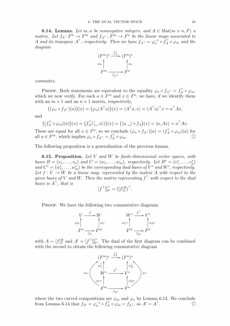
6. THE DUAL VECTOR SPACE 43
6.14. Lemma. Let m,n be nonnegative integers, and A ∈ Mat(m × n, F ) amatrix. Let fA : F n → Fm and fA> : Fm → F n be the linear maps associated toA and its transpose A>, respectively. Then we have fA> = ϕ−1n ◦ f>A ◦ ϕm and thediagram
(Fm)∗f>A // (F n)∗
Fm
fA>
//
ϕm
OO
F n
ϕn
OO
commutes.
Proof. Both statements are equivalent to the equality ϕn ◦ fA> = f>A ◦ ϕm,which we now verify. For each a ∈ Fm and x ∈ F n, we have, if we identify themwith an m× 1 and an n× 1 matrix, respectively,(
(ϕn ◦ fA>)(a))(x) =
(ϕn(A>a)
)(x) = 〈A>a, x〉 = (A>a)>x = a>Ax,
and((f>A ◦ ϕm)(a)
)(x) =
(f>A (〈 , a〉)
)(x) =
(〈a, 〉 ◦ fA
)(x) = 〈a,Ax〉 = a>Ax.
These are equal for all x ∈ F n, so we conclude (ϕn ◦ fA>)(a) = (f>A ◦ ϕm)(a) forall a ∈ Fm, which implies ϕn ◦ fA> = f>A ◦ ϕm. �
The following proposition is a generalisation of the previous lemma.
6.15. Proposition. Let V and W be finite-dimensional vector spaces, withbases B = (v1, . . . , vn) and C = (w1, . . . , wm), respectively. Let B∗ = (v∗1, . . . , v
∗n)
and C∗ = (w∗1, . . . , w∗m) be the corresponding dual bases of V ∗ and W ∗, respectively.
Let f : V → W be a linear map, represented by the matrix A with respect to thegiven bases of V and W. Then the matrix representing f> with respect to the dualbases is A>, that is
[f>]C∗
B∗ = ([f ]BC)>.
Proof. We have the following two commutative diagrams
Vf // W W ∗ f> // V ∗
F n
fA
//
ϕB
OO
Fm
ϕC
OO
Fm
fA′//
ϕC∗
OO
F n
ϕB∗
OO
with A = [f ]BC and A′ = [f>]C∗
B∗ . The dual of the first diagram can be combinedwith the second to obtain the following commutative diagram
(Fm)∗f>A // (F n)∗
W ∗ f> //
ϕ>C
OO
V ∗
ϕ>B
OO
Fm
ϕm
::
fA′//
ϕC∗
OO
F n
ϕB∗
OOϕn
dd
where the two curved compositions are ϕm and ϕn by Lemma 6.13. We concludefrom Lemma 6.14 that fA′ = ϕ−1n ◦ f>A ◦ ϕm = fA> , so A′ = A>. �
44 CONTENTS
Alternative proof. Let A = (aij)1≤i≤m,1≤j≤n; then
f(vj) =m∑i=1
aijwi .
We then have(f>(w∗i )
)(vj) = (w∗i ◦ f)(vj) = w∗i
(f(vj)
)= w∗i
( m∑k=1
akjwk
)= aij .
Since we always have, for φ ∈ V ∗, that φ =∑n
j=1 φ(vj)v∗j , this implies that
f>(w∗i ) =n∑j=1
aijv∗j .
Therefore the columns of the matrix representing f> with respect to the dualbases are exactly the rows of A. �
Note that for every invertible matrix P we have (P−1)> = (P>)−1; we will denotethis matrix by P−>.
6.16. Corollary. Let V be a finite-dimensional vector space, and let B =(v1, . . . , vn) and C = (w1, . . . , wn) be two bases of V. Let B∗ = (v∗1, . . . , v
∗n) and
C∗ = (w∗1, . . . , w∗n) be the corresponding dual bases. Then we have
[idV ∗ ]B∗
C∗ =([idV ]BC
)−>.
Proof. Using id>V = idV ∗ , we find from Proposition 6.15 that [idV ∗ ]C∗B∗ =(
[idV ]BC)>
. The statement now follows from the fact that the matrices [idV ∗ ]C∗B∗
and [idV ∗ ]B∗C∗ are each other’s inverses. �
This corollary is reflected in the matrices we use to change bases. If f : V → Vis an endomorphism and we set A = [f ]BB and A′ = [f ]CC , then for the matrixP = [idV ]BC we have A′ = PAP−1. The matrices A> = [f>]B
∗B∗ and A′> = [f>]C
∗C∗
are then related by A′> = (PAP−1)> = P−>A>P>.
As is to be expected, we have a compatibility between f>> and the canonicalmap αV .
6.17. Proposition. Let V and W be vector spaces, f : V → W a linear map.Then the following diagram commutes.
Vf //
αV��
W
αW��
V ∗∗f>> // W ∗∗
Proof. We have to show that f>> ◦αV = αW ◦ f . So let v ∈ V and ψ ∈ W ∗.Then
f>>(αV (v)
)(ψ) = (αV (v) ◦ f>)(ψ) = αV (v)
(f>(ψ)
)= αV (v)(ψ ◦ f) = (ψ ◦ f)(v)
= ψ(f(v)
)= αW
(f(v)
)(ψ) .
�

6. THE DUAL VECTOR SPACE 45
6.18. Proposition. Let V be a vector space. Then we have α>V ◦αV ∗ = idV ∗.If V is finite-dimensional, then α>V = α−1V ∗.
Proof. Let φ ∈ V ∗. Then for all v ∈ V we have
α>V(αV ∗(φ)
)(v) =
(αV ∗(φ) ◦ αV
)(v) = αV ∗(φ)
(αV (v)
)=(αV (v)
)(φ) = φ(v) ,
so α>V(αV ∗(φ)
)= φ, and α>V ◦ αV ∗ = idV ∗ .
Hence, αV ∗ is injective. If dimV <∞, then dimV ∗ = dimV <∞, and αV ∗ is anisomorphism; the relation we have shown then implies that α>V = α−1V ∗ . �
6.19. Corollary. Let V and W be finite-dimensional vector spaces. Then
Hom(V,W ) 3 f 7−→ f> ∈ Hom(W ∗, V ∗)
is an isomorphism.
Proof. By the observations made in Definition 6.11, the map is linear. Notethat by Propositions 6.12 and 6.18, we have (α−1W )> = (α>W )−1 = αW ∗ . This allowsus to conclude from Proposition 6.17 that the map
Hom(W ∗, V ∗) 3 g 7−→ α−1W ◦ g> ◦ αV ∈ Hom(V,W ) ,
is the inverse of the given map. Indeed,
α−1W ◦ f>> ◦ αV = f
and
(α−1W ◦ g> ◦ αV )> = α>V ◦ g>> ◦ (α−1W )> = α−1V ∗ ◦ g
>> ◦ αW ∗ = g .
�
The following lemma states that every linear form on a subspace U of a vectorspace V can be extended to a linear form on V . Note that if j : U → V isan inclusion map, then j> : V ∗ → U∗ is the restriction map that sends ϕ ∈ V ∗
to ϕ|U .
6.20. Lemma. Let V be a vector space and U ⊂ V a subspace. Let j : U ↪→ Vdenote the inclusion map. Then j> : V ∗ → U∗ is surjective.
Proof. Let U ′ ⊂ V be a complementary space of U (using Zorn’s Lemma ifV is infinite-dimensional), and π : V → U the projection onto U along U ′. Thatis, for v = u + u′ with u ∈ U and u′ ∈ U ′, we have π(v) = u. Then we haveπ ◦ j = idU , so j> ◦ π> = (π ◦ j)> = idU∗ , which implies that j> is surjective. �
6.21. Proposition. Let f : U → V and g : V → W be two linear maps ofvector spaces.
(1) If we have im f ⊂ ker g, then we have im g> ⊂ ker f>.(2) If we have ker g ⊂ im f , then we have ker f> ⊂ im g>.(3) If we have im f = ker g, then we have im g> = ker f>.
Proof. (1) Suppose im f ⊂ ker g. Then the composition g ◦f is the zeromap. Hence so is the dual of this composition, which is the compositionf> ◦ g> of the duals. This implies im g> ⊂ ker f>.

46 CONTENTS
(2) Write g as the composition g = j ◦ g with g : V → im g and j : im g → Wthe inclusion map. Then we have ker g = ker g. From Lemma 6.20 wefind that j> is surjective, so from g> = g> ◦ j> we obtain im g = im g.Hence it suffices to prove the statement with g instead of g, so withoutloss of generality, we may and will assume g is surjective.
Suppose ker g ⊂ im f . Take any ϕ ∈ ker f>, so f>(ϕ) = 0, that is,for all u ∈ U we have ϕ(f(u)) = 0. For each w ∈ W , there is a v ∈ Vwith g(v) = w, since g is surjective; for v, v′ ∈ V with g(v) = g(v′) = w,we have v − v′ ∈ ker g ⊂ im f , so there is a u ∈ U with f(u) = v − v′,and therefore ϕ(v) = ϕ(v− v′) +ϕ(v′) = ϕ(f(u)) +ϕ(v′) = ϕ(v′). Hence,there is a well-defined map ψ : W → F with ψ(g(v)) = ϕ(v) for all v ∈ V .To verify that ψ is linear, note that if w = g(v) and w′ = g(v′), then wehave w + w′ = g(v + v′), so
ψ(w + w′) = ϕ(v + v′) = ϕ(v) + ϕ(v′) = ψ(w) + ψ(w′);
The fact that ψ respects scalar multiplication follows similarly. We con-clude that ψ ∈ W ∗, and ϕ = g>(ψ) ∈ im g>, so ker f> ⊂ im g>.
(3) This follows from the previous statements.
�
6.22. Definition. A sequence
V0f1−→ V1
f2−→ · · · fn−→ Vn
of composable linear maps is called exact if for all indices 1 ≤ i < n we haveim fi = ker fi+1.
Proposition 6.21 states that if U → V → W is an exact sequence, then the inducedsequence W ∗ → V ∗ → U∗ is exact as well. Note that a linear map f : V → W is
injective if and only if the sequence 0→ Vf→ W is exact, while f is surjective if
and only if the sequence Vf→ W → 0 is exact.
6.23. Corollary. Let f : V → W be a linear map of vector spaces. If f isinjective, then f> is surjective. If f is surjective, then f> is injective.
Proof. If f is injective, then the sequence 0 → Vf→ W is exact. Then by
Proposition 6.21 the sequence W ∗ f>→ V ∗ → 0 is exact, so f> is surjective. As an
alternative proof, we could have also written f as the composition f = j ◦ f of theisomorphism f : V → im f induced by f , and the inclusion j : im f → W ; then byProposition 6.12 and Lemma 6.20, the map f> = f> ◦ j> is the composition of asurjection and an isomorphism, and thus surjective.
If f is surjective, then the sequence Vf→ W → 0 is exact. Then by Proposi-
tion 6.21 the sequence 0→ W ∗ f>→ V ∗ is exact, so f> is injective. �
6.24. Definition. Let A ∈ Mat(m×n, F ) be a matrix. A kernel matrix of Ais a matrix whose columns span the kernel of A.
If B is a kernel matrix of A, then we have im fB = ker fA. By Proposition 6.21,this implies im f>A = ker f>B ⊂ (F n)∗. Applying ϕ−1n , we obtain the equalityim fA> = ker fB> by Lemma 6.14. This shows that A> is a kernel matrix of B>.

6. THE DUAL VECTOR SPACE 47
6.25. Proposition. Let f : V → W be a linear map of finite-dimensionalvector spaces. Then we have
dim im f = dim im f>
and
dimV − dim ker f = dimW − dim ker f>.
Proof. The map f is the composition of the surjection f : V → im f inducedby f and the inclusion j : im f → W . By Corollary 6.23, the dual map f> isthe composition of the surjective map j> : W ∗ → (im f)∗ and the injective map
f> : (im f)∗ → V ∗. We conclude im f> = im f> and hence
dim im f> = dim im f> = dim(im f)∗ = dim im f,
which proves the first equality. We also conclude ker f> = ker j>, so we find
dim ker f> = dim ker j> = dimW ∗ − dim(im f)∗
= dimW − dim im f = dimW − (dimV − dim ker f),
which proves the second equality. �
6.26. Remark. The equality of dimensions dim im(f>) = dim im(f) is, byProp. 6.15, equivalent to the statement “row rank equals column rank” for matri-ces.
Note that [BR2] claims (in Theorem 7.8) that we also have dim ker(f>) = dim ker(f).However, this is false unless dimV = dimW !
Next, we study how subspaces relate to dualization.
6.27. Definition. Let V be a vector space and S ⊂ V a subset. Then
S◦ = {φ ∈ V ∗ : φ(v) = 0 for all v ∈ S} ⊂ V ∗
is called the annihilator of S.
S◦ is a linear subspace of V ∗, since we can write
S◦ =⋂v∈S
ker(αV (v)
).
Trivial examples are {0V }◦ = V ∗ and V ◦ = {0V ∗}.
6.28. Remark. As we have seen before, if U is a subspace of a vector space V ,and j : U → V is the inclusion map, then j> : V ∗ → U∗ is the restriction map,which sends each linear form ψ ∈ V ∗ to its restriction ψ|U ; we have
U◦ = ker j>.

48 CONTENTS
6.29. Theorem. Let V be a finite-dimensional vector space, U ⊂ V a linearsubspace. Then we have
dimU + dimU◦ = dimV and αV (U) = U◦◦ .
Proof. As in Remark 6.28, the dual of the inclusion j : U ↪→ V is a surjectivemap V ∗ → U∗, of which the kernel is U◦. Hence, we have dimU◦ + dimU∗ =dimV ∗, even if V were not finite-dimensional. Because V is finite-dimensional, wehave dimV = dimV ∗ and dimU = dimU∗, so the first equality follows. Applyingit to U◦, we obtain dimU = dimU◦◦.
For the second equality, note that U◦ consists of all the linear forms on V thatvanish on U . Hence, for every u ∈ U , the evaluation map evu : V ∗ → F sendingϕ ∈ V ∗ to ϕ(u) sends all of U◦ to 0. This implies that the element αV (u) =evu ∈ V ∗∗ is contained in U◦◦, so we have αV (U) ⊂ U◦◦, even if V were not finite-dimensional. Because V is finite-dimensional, we have dimαV (U) = dimU =dimU◦◦, so the inclusion αV (U) ⊂ U◦◦ is an equality. �
The theorem implies that we have U◦◦ = U if we identify V and V ∗∗ via αV .
6.30. Theorem. Let f : V → W be a linear map of vector spaces. Then wehave (
ker(f))◦
= im(f>) and(im(f)
)◦= ker(f>).
Proof. Let j : ker f → V be the inclusion map. Apply Proposition 6.21 tothe exact sequence
ker fj→ V
f→ W
to get the exact sequence
W ∗ f>−→ V ∗j>−→ (ker f)∗ ,
which implies im f> = ker j> = (ker f)◦, which proves the first equality. For thesecond equality, let i : im f → W denote the inclusion map, and write f as thecomposition f = i ◦ f with f : V → im f induced by f . Then f> = f> ◦ i>, andsince f> is injective, we obtain ker f> = ker i> = (im f)◦. �
6.31. Interpretation in Terms of Matrices. Let us consider the vectorspaces V = F n and W = Fm and a linear map f : V → W . Then f is representedby a matrix A, and the image of f is the column space of A, i.e., the subspaceof Fm spanned by the columns of A. We identify V ∗ = (F n)∗ and W ∗ = (Fm)∗
with F n and Fm via the dual bases consisting of the coordinate maps (see thetext above Lemma 6.13). Then for x ∈ W ∗, we have x ∈ (im(f))◦ if and only ifx>y = 〈x, y〉 = 0 for all columns y of A, which is the case if and only if x>A = 0.This is equivalent to A>x = 0, which says that x ∈ ker(f>) — remember that A>
represents f> : W ∗ → V ∗.

7. NORMS ON REAL VECTOR SPACES 49
Exercises.
(1) Define φi : Rn → R by φi(x1, . . . , xn) = x1+x2+ · · ·+xi for i = 1, 2, . . . n.Show that φ1, . . . , φn is a basis of (Rn)∗, and compute its dual basis ofRn.
(2) Let V be an n-dimensional vector space, let v1, . . . , vn ∈ V and letφ1, . . . , φn ∈ V ∗. Show that det((φi(vj))i,j) is non-zero if and only ifv1, . . . , vn is a basis of V and φ1, . . . , φn is a basis of V ∗.
(3) Let V be the 3-dimensional vector space of polynomial functions R→ Rof degree at most 2. In each of the following cases, we define φi ∈ V ∗ fori = 0, 1, 2. In each case, indicate whether φ0, φ1, φ2 is a basis of V ∗, andif so, give the dual basis of V .(a) φi(f) = f(i)(b) φi(f) = f (i)(0), i.e., the ith derivative of f evaluated at 0.(c) φi(f) = f (i)(1)
(d) φi(f) =∫ i−1 f(x)dx
(4) For each positive integer n show that there are constants a1, a2, . . . , an sothat
1∫0
f(x)exdx =n∑i=1
aif(i)
for all polynomial functions f : R→ R of degree less than n.(5) Suppose V is a finite dimensional vector space and W is a subspace. Let
f : V → V be a linear map so that f(w) = w for w ∈ W . Show thatfT (v∗)− v∗ ∈ W o for all v∗ ∈ V ∗.
Conversely, if you assume that fT (v∗)− v∗ ∈ W o for all v∗ ∈ V ∗, canyou show that f(w) = w for w ∈ W?
(6) * Let V be a finite-dimensional vector space and let U ⊂ V and W ⊂ V ∗
be subspaces. We identify V and V ∗∗ via αV (so W ◦ ⊂ V ). Show that
dim(U◦ ∩W ) + dimU = dim(U ∩W ◦) + dimW .
(7) Let φ1, . . . , φn ∈ (Rn)∗. Prove that the solution set C of the linear in-equalities φ1(x) ≥ 0, . . . , φn(x) ≥ 0 has the following properties:(a) α, β ∈ C =⇒ α + β ∈ C .
(b) α ∈ C, t ∈ R≥0 =⇒ tα ∈ C.
(c) If φ1, . . . , φn form a basis of (Rn)∗, then
C ={t1α1 + . . .+ tnαn : ti ∈ R≥0,∀i ∈ {1, . . . , n}
},
where α1, . . . , αn is the basis of Rn dual to φ1, . . . , φn.
7. Norms on Real Vector Spaces
The following has some relevance for Analysis.
7.1. Definition. Let V be a real vector space. A norm on V is a map V → R,usually written x 7→ ‖x‖, such that
(i) ‖x‖ ≥ 0 for all x ∈ V , and ‖x‖ = 0 if and only if x = 0;
(ii) ‖λx‖ = |λ|‖x‖ for all λ ∈ R, x ∈ V ;
(iii) ‖x+ y‖ ≤ ‖x‖+ ‖y‖ for all x, y ∈ V (triangle inequality).

50 CONTENTS
7.2. Examples. If V = Rn, then we have the following standard examples ofnorms.
(1) The maximum norm:
‖(x1, . . . , xn)‖∞ = max{|x1|, . . . , |xn|} .
(2) The euclidean norm (see Section 9 below):
‖(x1, . . . , xn)‖2 =√x21 + . . . x2n .
(3) The sum norm (or 1-norm):
‖(x1, . . . , xn)‖1 = |x1|+ · · ·+ |xn| .
7.3. Remark. A norm on a real vector space V induces a metric: we set
d(x, y) = ‖x− y‖ ,
then the axioms of a metric (positivity, symmetry, triangle inequality) follow fromthe properties of a norm.
Recall that the usual Euclidean topology on Rn is induced by the Euclidean metricgiven by d(x, y) = ‖x − y‖2 for all x, y ∈ Rn. With respect to this topology, wehave the following result.
7.4. Lemma. Every norm on Rn is continuous (as a map from Rn to R).
Proof. Note that the maximum norm on Rn is bounded from above by theEuclidean norm:
max{|xj| : j ∈ {1, . . . , n}} ≤√x21 + · · ·+ x2n .
Let ‖ · ‖ be a norm, and set C =∑n
j=1 ‖ej‖, where e1, . . . , en is the canonical basis
of Rn. Then for x = (x1, . . . , xn) ∈ Rn we have
‖x‖ = ‖(x1, . . . , xn)‖ = ‖x1e1 + · · ·+ xnen‖ ≤ ‖x1e1‖+ · · ·+ ‖xnen‖= |x1|‖e1‖+ · · ·+ |xn|‖en‖ ≤ max{|x1|, . . . , |xn|} · C ≤ ‖x‖2 · C .
From the triangle inequality, we then get∣∣‖x‖ − ‖y‖∣∣ ≤ ‖x− y‖ ≤ C · ‖x− y‖2 .
So for any ε > 0, if ‖x− y‖2 < ε/C, then∣∣‖x‖ − ‖y‖∣∣ < ε. �
7.5. Definition. Let V be a real vector space, x 7→ ‖x‖1 and x 7→ ‖x‖2 twonorms on V (any norms, not necessarily those of Example 7.2!). The two normsare said to be equivalent, if there are C1, C2 > 0 such that
C1‖x‖1 ≤ ‖x‖2 ≤ C2‖x‖1 for all x ∈ V .
7. NORMS ON REAL VECTOR SPACES 51
7.6. Theorem. On a finite-dimensional real vector space, all norms are equiv-alent.
Proof. Without loss of generality, we can assume that our space is Rn, andwe can assume that one of the norms is the euclidean norm ‖ · ‖2 defined above.Let S ⊂ Rn be the unit sphere, i.e., S = {x ∈ Rn : ‖x‖2 = 1}. We know fromAnalysis that S is compact (it is closed as the zero set of the continuous functionx 7→ x21 + · · · + x2n − 1 and bounded). Let ‖ · ‖ be another norm on Rn. Thenx 7→ ‖x‖ is continuous by Lemma 7.4, hence it attains a maximum C2 and aminimum C1 on S. Then C2 ≥ C1 > 0 (since 0 /∈ S). Now let 0 6= x ∈ V , andlet e = ‖x‖−12 x; then ‖e‖2 = 1, so e ∈ S. This implies that C1 ≤ ‖e‖ ≤ C2, andtherefore
C1‖x‖2 ≤ ‖x‖2 · ‖e‖ ≤ C2‖x‖2 .From ‖x‖2 · ‖e‖ =
∥∥‖x‖2e∥∥ = ‖x‖ we conclude C1‖x‖2 ≤ ‖x‖ ≤ C2‖x‖2. So everynorm is equivalent to ‖ · ‖2, which implies the claim, since equivalence of norms isan equivalence relation. �
7.7. Examples. If V is infinite-dimensional, then the statement of the theo-rem is no longer true. As a simple example, consider the space of finite sequences(an)n≥0 (such that an = 0 for n sufficiently large). Then we can define norms ‖·‖1,‖·‖2, ‖·‖∞ as in Examples 7.2, but they are pairwise inequivalent now — considerthe sequences sn = (1, . . . , 1, 0, 0, . . . ) with n ones, then ‖sn‖1 = n, ‖sn‖2 =
√n
and ‖sn‖∞ = 1.
Here is a perhaps more natural example. Let V be the vector space C([0, 1]) ofreal-valued continuous functions on the unit interval. We can define norms
‖f‖1 =
1∫0
|f(x)| dx , ‖f‖2 =
√√√√√ 1∫0
f(x)2 dx , ‖f‖∞ = max{|f(x)| : x ∈ [0, 1]}
in a similar way as in Examples 7.2, and again they are pairwise inequivalent.Taking f(x) = xn, we have
‖f‖1 =1
n+ 1, ‖f‖2 =
1√2n+ 1
, ‖f‖∞ = 1 .
Exercises.
Let V and W be normed vector spaces over R. For a linear map f : V → W set
‖f‖ = supx∈V, ‖x‖=1
‖f(x)‖ .
(1) Consider V = Rn with the standard inner product and the norm ‖ · ‖2.Suppose that f : V → V is a diagonalizable map whose eigenspaces areorthogonal (i.e., V has an orthogonal basis consisting of eigenvectors off). Show that ‖f‖ as defined above is equal to the largest absolute valueof an eigenvalue of f .
(2) (a) Show that B(V,W ) = {f ∈ Hom(V,W ) : ‖f‖ < ∞} is a subspaceof Hom(V,W ), and that ‖ · ‖ is a norm on B(V,W ).
(b) Show that B(V,W ) = Hom(V,W ) if V is finite-dimensional.(c) Taking V = W above, we obtain a norm on B(V, V ). Show that‖f ◦ g‖ ≤ ‖f‖ · ‖g‖ for all f, g ∈ B(V, V ).

52 CONTENTS
(3) Consider the rotation map f : R2 → R2 which rotates the plane by 45degrees. For any norm on R2 the previous exercise defines a norm ‖f‖.Show that ‖f‖ = 1 when we take the standard euclidean norm ‖ · ‖2 onR2. What is ‖f‖ when we take the maximum norm ‖ · ‖∞ on R2?
(4) Consider the vector space V of polynomial functions [0, 1]→ R with thesup-norm: ‖f‖ = sup0≤x≤1 |f(x)|. Consider the functional φ ∈ V ∗ definedby φ(f) = f ′(0). Show that φ 6∈ B(V,R). [Hint: consider the polynomials(1− x)n for n = 1, 2, . . ..]
(5) What is the sine of the matrix
(π π0 π
)?
8. Bilinear Forms
We have already seen multilinear maps when we were discussing the determinantin Linear Algebra I. Let us remind ourselves of the definition in the special casewhen we have two arguments.
8.1. Definition. Let V1, V2 and W be F -vector spaces. A map φ : V1×V2 →W is bilinear if it is linear in both arguments, i.e.
∀λ, λ′ ∈ F, x, x′ ∈ V1, y ∈ V2 : φ(λx+ λ′x′, y) = λφ(x, y) + λ′φ(x′, y) and
∀λ, λ′ ∈ F, x ∈ V1, y, y′ ∈ V2 : φ(x, λy + λ′y′) = λφ(x, y) + λ′φ(x, y′) .
When W = F is the field of scalars, φ is called a bilinear form.
If V1 = V2 = V and W = F , then φ is a bilinear form on V. It is symmetric ifφ(x, y) = φ(y, x) for all x, y ∈ V , and alternating if φ(x, x) = 0 for all x ∈ V . Thelatter property implies that φ is skew-symmetric, i.e. φ(x, y) = −φ(y, x) for allx, y ∈ V. To see this, consider
0 = φ(x+ y, x+ y) = φ(x, x) + φ(x, y) + φ(y, x) + φ(y, y) = φ(x, y) + φ(y, x) .
The converse holds if char(F ) 6= 2, since (taking x = y)
0 = φ(x, x) + φ(x, x) = 2φ(x, x) .
We denote by Bil(V,W ) the set of all bilinear forms V ×W → F , and by Bil(V )the set of all bilinear forms on V. These sets are F -vector spaces in the usual way,by defining addition and scalar multiplication point-wise.
8.2. Examples. The standard ‘dot product’ on Rn is a symmetric bilinearform on Rn.
The map that sends(( ab ) , ( cd )
)∈ R2 × R2 to | a cb d | = ad − bc is an alternating
bilinear form on R2.
The map (A,B) 7→ Tr(A>B) is a symmetric bilinear form on Mat(m× n, F ).
If K : [0, 1]2 → R is continuous, then the following defines a bilinear form on thespace of continuous real-valued functions on [0, 1]:
(f, g) 7−→1∫
0
1∫0
K(x, y)f(x)g(y) dx dy .
Evaluation defines a bilinear form on V × V ∗: (v, φ) 7−→ φ(v).

8. BILINEAR FORMS 53
8.3. Definition. A bilinear form φ : V ×W → F induces linear maps
φL : V −→ W ∗, v 7→(w 7→ φ(v, w)
)and φR : W −→ V ∗, w 7→
(v 7→ φ(v, w)
).
The subspace ker(φL) ⊂ V is called the left kernel of φ; it is the set of all v ∈ Vsuch that φ(v, w) = 0 for all w ∈ W . Similarly, the subspace ker(φR) ⊂ W iscalled the right kernel of φ. The bilinear form φ is said to be nondegenerate if φLand φR are isomorphisms.
8.4. Remark. If φ : V ×W → F is a nondegenerate bilinear form, then Vand W have the same finite dimension (Exercise, cf. Remark 6.6).
8.5. Lemma. Let φ : V ×W → F be a bilinear form with V or W finite-dimensional. Then φ is nondegenerate if and only if both its left and right kernelare trivial.
Proof. First, by the definition of bilinear forms, the maps w 7→ φ(v, w) (forany fixed v ∈ V ) and v 7→ φ(v, w) (for any fixed w ∈ W ) are linear, so φL and φRare well-defined as maps into W ∗ and V ∗, respectively. Then using the definitionof bilinearity again, we see that φL and φR are themselves linear maps.
To prove the last statement, first observe that the left and right kernels are cer-tainly trivial when φL and φR are isomorphisms. For the converse statement,first suppose that W is finite-dimensional. Assume that the left and right kernelsare trivial. Then φL is injective, and since W is finite-dimensional, we obtaindimV ≤ dimW ∗ = dimW , so V is finite-dimensional as well. From φR beinginjective, we similarly get dimW ≤ dimV , so dimV = dimW and φL and φR areisomorphisms. The case that V is finite-dimensional works analogously. �
8.6. Example. For the ‘evaluation pairing’ ev : V × V ∗ → F , we find thatthe map evL : V → V ∗∗ is αV , and evR : V ∗ → V ∗ is the identity. So this bilinarform ev is nondegenerate if and only if αV is an isomorphism, which is the case ifand only if V is finite-dimensional (see Remark 6.6).
8.7. Example. The standard scalar (dot) product φ on F n given by φ(v, w) =〈v, w〉 is a nondegenerate symmetric bilinear form. In fact, here φL equals ϕn asdefined in the paragraph above Lemma 6.13: it sends the standard basis vector ejto the jth coordinate map in (F n)∗, so it maps a basis to a basis and is thereforean isomorphism.
8.8. Remarks.
(1) The bilinear form φ : V × V → F is symmetric if and only if φR = φL.
(2) Suppose V and W have the same finite dimension. If φ : V ×W → Fis a bilinear form, then φ is nondegenerate if and only if its left kernel istrivial (if and only if its right kernel is trivial).
Indeed, in this case, dimW ∗ = dimV , so if φL is injective, it is alsosurjective, hence an isomorphism. But then the identity φR = φ>L ◦ αW(which we leave as an exercise for the reader) is an isomorphism as well.If φR is injective, then we use the identity φL = φ>R ◦ αV instead.
In fact, we can say a little bit more.

54 CONTENTS
8.9. Proposition. Let V and W be F -vector spaces. There is an isomor-phism
βV,W : Bil(V,W ) −→ Hom(V,W ∗) , φ 7−→ φL
with inverse given by
f 7−→((v, w) 7→ (f(v))(w)
).
Proof. We leave the (by now standard) proof that the given maps are linearas an exercise. It remains to check that they are inverses of each other. Call thesecond map γV,W . So let φ : V × W → F be a bilinear form. Then γV,W (φL)sends (v, w) to (φL(v))(w) = φ(v, w), so γV,W ◦ βV,W is the identity. Conversely,let f ∈ Hom(V,W ∗), and set φ = γV,W (f). Then for v ∈ V , the linear form φL(v)sends w to (φL(v))(w) = φ(v, w) = (f(v))(w), so φL(v) = f(v) for all v ∈ V , henceφL = f . This shows that βV,W ◦ γV,W is also the identity map. �
If V = W , we write βV : Bil(V )→ Hom(V, V ∗) for this isomorphism.
8.10. Example. Let V now be finite-dimensional. We see that a nondegener-ate bilinear form φ on V allows us to identify V with V ∗ via the isomorphism φL.Conversely, if we fix a basis B = (v1, . . . , vn), we also obtain an isomorphismι : V → V ∗ by sending vj to v∗j , where B∗ = (v∗1, . . . , v
∗n) is the dual basis of V ∗.
What is the bilinear form φ : V × V → F corresponding to this map? We have,for v =
∑nj=1 λjvj, w =
∑nj=1 µjvj,
φ(v, w) =(ι(v)
)(w) =
(ι( n∑j=1
λjvj
))( n∑k=1
µkvk
)=( n∑j=1
λjv∗j
)( n∑k=1
µkvk
)=
n∑j,k=1
λiµk v∗j (vk) =
n∑j,k=1
λiµkδjk =n∑j=1
λjµj .
This is just the standard dot product if we identify V with F n using the givenbasis; it is a symmetric bilinear form on V.
Alternatively, we note that ϕB∗ = ι ◦ϕB, so we obtain the following commutativediagram by Lemma 6.13.
Vι // V ∗
ϕ>B��
F n
ϕB
OOϕB∗
;;
ϕn// (F n)∗
Hence, indeed, if we identify V with F n through ϕB (and likewise V ∗ with (F n)∗
through ϕ>B), then ι : V → V ∗ corresponds to the map ϕn : F n → (F n)∗, whichsends a ∈ F n to the linear form 〈 , a〉. As we have seen in Example 8.7, this mapcorresponds to the bilinear form that is the usual scalar (dot) product.
8.11. Proposition. Let V,W be a F -vector spaces, and let φ : V ×W → Fbe a nondegenerate bilinear form. Then for every linear form ψ ∈ W ∗ there is aunique v ∈ V such that for every w ∈ W we have ψ(w) = φ(v, w).
Proof. The condition that for every w ∈ W we have ψ(w) = φ(v, w) isequivalent with the equality ψ = φ(v, ·), which means that ψ = φL(v). The claimnow follows from the fact that φL : V → W ∗ is an isomorphism. �

8. BILINEAR FORMS 55
8.12. Example. Let V be the real vector space of polynomials of degree atmost 2. Then
φ : V × V → R, (p, q) 7−→1∫
0
p(x)q(x) dx
is a bilinear form on V. It is nondegenerate since for p 6= 0, we have φ(p, p) > 0.Evaluation at zero p 7→ p(0) defines a linear form on V, which by Proposition 8.11must be representable in the form p(0) = φ(q, p) for some q ∈ V. To find q, wehave to solve a linear system:
φ(a0 + a1x+ a2x2, b0 + b1x+ b2x
2)
= a0b0 +1
2(a0b1 + a1b0) +
1
3(a0b2 + a1b1 + a2b0) +
1
4(a1b2 + a2b2) +
1
5a2b2 ,
and we want to find a0, a1, a2 such that this is always equal to b0. This leads to
a0 +1
2a1 +
1
3a2 = 1 ,
1
2a0 +
1
3a1 +
1
4a2 = 0 ,
1
3a0 +
1
4a1 +
1
5a2 = 0
so q(x) = 9− 36x+ 30x2, and
p(0) =
1∫0
(9− 36x+ 30x2)p(x) dx .
8.13. Representation by Matrices. Let φ : F n × Fm → F be a bilinearform. Then we can represent φ by a matrix A = (aij) ∈ Mat(m × n, F ), withentries aij = φ(ej, ei). In terms of column vectors x ∈ F n and y ∈ Fm, we have
φ(x, y) = y>Ax .
Similarly, if V and W are finite-dimensional F -vector spaces, and we fix basesB = (v1, . . . , vn) and C = (w1, . . . , wm) of V and W , respectively, then any bilinearform φ : V ×W → F is given by a matrix relative to these bases, by identifyingV and W with F n and Fm in the usual way, that is, through the isomorphismsϕB : F n → V and ϕC : Fm → W . If A = (aij) is the matrix as above, thenaij = φ(vj, wi). If v = x1v1 + · · ·+ xnvn and w = y1w1 + · · ·+ ymwm, then
φ(v, w) =m∑i=1
n∑j=1
aijxjyi .
8.14. Proposition. Let V and W be finite-dimensional F -vector spaces. Picktwo bases B = (v1, . . . , vn) and B′ = (v′1, . . . , v
′n) of V and two bases C =
(w1, . . . , wm) and C ′ = (w′1, . . . , w′m) of W . Let A be the matrix representing the
bilinear form φ : V ×W → F with respect to B and C, and let A′ be the matrixrepresenting φ with respect to B′ and C ′. Then for P = [idV ]B
′B and Q = [idW ]C
′C
we haveA′ = Q>AP .
Proof. Let x′ ∈ F n be the coefficients of v ∈ V w.r.t. the new basis B′. Thenx = Px′, where x represents v w.r.t. the old basis B. Similary for y′, y ∈ Fm
representing w ∈ W w.r.t. the two bases, we have y = Qy′. So
y′>A′x′ = φ(v, w) = y>Ax = y′
>Q>APx′ ,
which implies the claim. �

56 CONTENTS
V ×W φ // F 3 y>Ax = y′>A′x′
F n × Fm
(ϕB ,ϕC)
OO 99
(x, y)6
::
A′ = Q>AP
F n × Fm
(P,Q)
OO(ϕB′ ,ϕC′ )
;; BB
(x′, y′)2
88
_
OO
A =(φ(vj, wi)
)i,j
In particular, if φ is a bilinear form on the n-dimensional vector space V, then φis represented (w.r.t. any given basis) by a square matrix A ∈ Mat(n, F ). If wechange the basis, then the new matrix will be B = P>AP , with P ∈ Mat(n, F )invertible. Matrices A and B such that there is an invertible matrix P ∈ Mat(n, F )such that B = P>AP are called congruent.
8.15. Remark. Let A be an m × n matrix over F . Then the associatedbilinear form
F n × Fm → F, (x, y) 7→ y>Ax
can also be expressed using the standard dot products on Fm and F n, both denotedby 〈 , 〉, as we have
〈y, Ax〉 = y>Ax = (A>y)>x = 〈A>y, x〉.
8.16. Example. Let V be the real vector space of polynomials of degree lessthan n, and consider again the symmetric bilinear form
φ(p, q) =
1∫0
p(x)q(x) dx .
With respect to the standard basis (1, x, . . . , xn−1), it is represented by the “Hilbertmatrix” Hn =
(1
i+j−1
)1≤i,j≤n.
For completeness, we summarize in one commutative diagram the ways to associatea matrix to linear maps and bilinear forms. Let V and W be finite-dimensionalvector spaces, with bases B and C, respectively. Let C∗ denote the dual basisof W ∗. Also set ι = ϕC∗ ◦ ϕ−1C : W → W ∗, which sends the i-th basis vector of Cto the i-th basis vector of C∗. Recall that ϕm = ϕ>C ◦ ϕC∗ : Fm → (Fm)∗ sendsa ∈ Fm to 〈a, 〉. Then all maps in the following diagram are isomorphisms.
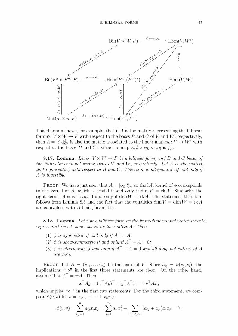
8. BILINEAR FORMS 57
Bil(V ×W,F ) Hom(V,W ∗)
Bil(F n × Fm, F ) Hom(F n, (Fm)∗) Hom(V,W )
Mat(m× n, F ) Hom(F n, Fm)
φ 7−→ φL
φ ◦(ϕB
,ϕC) ←−[ φ
ϕ>C◦h◦ϕB←−
[ h
ϕ−1
C∗◦h◦ϕB←−[h
φ 7−→ φL
ϕ−1C
◦ g◦ϕB←−
[ g
g7−→
ι◦g
A 7−→ (x 7→Ax)
A7−→
(x7→〈Ax, 〉)
A7−→
((x,y)7→
y> Ax)
f7−→
ϕm◦f
This diagram shows, for example, that if A is the matrix representing the bilinearform φ : V ×W → F with respect to the bases B and C of V and W , respectively,then A = [φL]BC∗ is also the matrix associated to the linear map φL : V → W ∗ withrespect to the bases B and C∗, since the map ϕ−1C∗ ◦ φL ◦ ϕB is fA.
8.17. Lemma. Let φ : V ×W → F be a bilinear form, and B and C bases ofthe finite-dimensional vector spaces V and W , respectively. Let A be the matrixthat represents φ with respect to B and C. Then φ is nondegenerate if and only ifA is invertible.
Proof. We have just seen that A = [φL]BC∗ , so the left kernel of φ correspondsto the kernel of A, which is trivial if and only if dimV = rkA. Similarly, theright kernel of φ is trivial if and only if dimW = rkA. The statement thereforefollows from Lemma 8.5 and the fact that the equalities dimV = dimW = rkAare equivalent with A being invertible. �
8.18. Lemma. Let φ be a bilinear form on the finite-dimensional vector space V,represented (w.r.t. some basis) by the matrix A. Then
(1) φ is symmetric if and only if A> = A;
(2) φ is skew-symmetric if and only if A> + A = 0;
(3) φ is alternating if and only if A> + A = 0 and all diagonal entries of Aare zero.
Proof. Let B = (v1, . . . , vn) be the basis of V. Since aij = φ(vj, vi), theimplications “⇒” in the first three statements are clear. On the other hand,assume that A> = ±A. Then
x>Ay = (x>Ay)> = y>A>x = ±y>Ax ,which implies “⇐” in the first two statements. For the third statement, we com-pute φ(v, v) for v = x1v1 + · · ·+ xnvn:
φ(v, v) =n∑
i,j=1
aijxixj =n∑i=1
aiix2i +
∑1≤i<j≤n
(aij + aji)xixj = 0 ,

58 CONTENTS
since the assumption implies that both aii and aij + aji vanish. �
8.19. Definition. Let φ : V ×W → F be a bilinear form. For any subspaceU ⊂ W we set
U⊥ = {v ∈ V : φ(v, u) = 0 for all u ∈ U} .
For any subspace U ⊂ V we set
U⊥ = {w ∈ W : φ(u,w) = 0 for all u ∈ U} .
In both cases we call U⊥ the subspace orthogonal to U (with respect to φ).
8.20. Remark. Note that for a subspace U ⊂ W , the set U⊥ is indeed asubspace, as it is the kernel of the composition of φL : V → W ∗ with the restrictionmap resWU : W ∗ → U∗ that sends ψ ∈ W ∗ to the restriction ψ|U . Similarly, for asubspace U ⊂ V , the subspace U⊥ is the kernel of the composition of φR : W → V ∗
with the restriction map resVU : V ∗ → U∗. Moreover, as the kernel of resVU is theannihilator U◦, we also find U⊥ = φ−1R (U◦).
8.21. Example. Let V be a vector space over F , and consider the bilinearform ev : V × V ∗ → F of Example 8.6. Let U ⊂ V be a subspace. Then theorthogonal subspace U⊥ with respect to ev consists of all f ∈ V ∗ that satisfyf(u) = ev(u, f) = 0 for all u ∈ U . This means that the subspace U⊥ = U◦ isthe annihilator of U . Note that this is a special case of Remark 8.20, as we haveevR = idV ∗ (see Example 8.6).
8.22. Lemma. Let φ : V ×W → F be a nondegenerate bilinear form, with V ,W finite-dimensional vector spaces. Let U be a subspace of either V or W . Thenwe have dimU + dimU⊥ = dimV = dimW . Moreover, we have (U⊥)⊥ = U .
Proof. From Remark 8.4 we recall dimV = dimW . First suppose U ⊂ W .By Remark 6.28, the restriction map resWU : W ∗ → U∗ is surjective. So is the mapφL : V → W ∗, and therefore so is the composition V → U∗. The kernel of thiscomposition is U⊥, so we obtain dimV = dimU⊥ + dimU∗ = dimU⊥ + dimU .The case U ⊂ V follows similarly by considering the composition of φR with therestriction map resVU , thus proving the identity dimU + dimU⊥ = dimV in allcases. Applying this identity to U⊥ as well, we find dim(U⊥)⊥ = dimU . For allu ∈ U and all w ∈ U⊥, we have φ(u,w) = 0, so there is an inclusion U ⊂ (U⊥)⊥ ofsubspaces of the same finite dimension. Hence, this inclusion is an equality. �
We leave it to the reader to find an example of a bilinear form φ on a finite-dimensional vector space V that is degenerate and for which there is a subspaceU ⊂ V with (U⊥)⊥ 6= U .
As with endomorphisms, we can also split bilinear forms into direct sums in somecases.

8. BILINEAR FORMS 59
8.23. Definition. If V = U ⊕ U ′, φ is a bilinear form on V , ψ and ψ′ arebilinear forms on U and U ′, respectively, and for u1, u2 ∈ U , u′1, u
′2 ∈ U ′, we have
φ(u1 + u′1, u2 + u′2) = ψ(u1, u2) + ψ′(u′1, u′2) ,
then φ is the orthogonal direct sum of ψ and ψ′.
Given V = U⊕U ′ and φ, this is the case if and only if φ(u, u′) = 0 and φ(u′, u) = 0for all u ∈ U , u′ ∈ U ′ (and then ψ = φ|U×U , ψ′ = φ|U ′×U ′).This can be generalized to an arbitrary number of summands.
If V is finite-dimensional and we represent φ by a matrix with respect to a basisthat is compatible with the splitting, then the matrix will be block diagonal.
8.24. Proposition. Let φ be a symmetric bilinear form on V, and let U ⊂ Vbe a linear subspace such that φ|U×U is nondegenerate. Then V = U ⊕ U⊥, and φsplits accordingly as an orthogonal direct sum.
When the restriction of φ to U × U is nondegenerate, we call U⊥ the orthogonalcomplement of U .
Proof. We have to check a number of things. First, U ∩ U⊥ = {0} sincev ∈ U ∩ U⊥ implies φ(v, u) = 0 for all u ∈ U , but φ is nondegenerate on U , so vmust be zero. Second, U + U⊥ = V : let v ∈ V, then U 3 u 7→ φ(v, u) is a linearform on U , and since φ is nondegenerate on U , by Proposition 8.11 there must beu′ ∈ U such that φ(v, u) = φ(u′, u) for all u ∈ U . This means that φ(v−u′, u) = 0for all u ∈ U , hence v − u′ ∈ U⊥, and we see that v = u′ + (v − u′) ∈ U + U⊥ asdesired. So we have V = U ⊕U⊥. The last statement is clear, since by definition,φ is zero on U × U⊥. �
Here is a first and quite general classification result for symmetric bilinear forms:they can always be diagonalized.
8.25. Lemma. Assume that char(F ) 6= 2, let V be an F -vector space and φ asymmetric bilinear form on V. If φ 6= 0, then there is v ∈ V such that φ(v, v) 6= 0.
Proof. If φ 6= 0, then there are v, w ∈ V such that φ(v, w) 6= 0. Note thatwe have
0 6= 2φ(v, w) = φ(v, w) + φ(w, v) = φ(v + w, v + w)− φ(v, v)− φ(w,w) ,
so at least one of φ(v, v), φ(w,w) and φ(v + w, v + w) must be nonzero. �
8.26. Theorem. Assume that char(F ) 6= 2, let V be a finite-dimensionalF -vector space and φ a symmetric bilinear form on V. Then there is a basis(v1, . . . , vn) of V such that φ is represented by a diagonal matrix with respect tothis basis.
Equivalently, every symmetric matrix A ∈ Mat(n, F ) is congruent to a diagonalmatrix.
Proof. If φ = 0, there is nothing to prove. Otherwise, we proceed by induc-tion on the dimension n. Since φ 6= 0, by Lemma 8.25, there is v1 ∈ V such thatφ(v1, v1) 6= 0 (in particular, n ≥ 1). Let U = L(v1), then φ is nondegenerate on U .By Prop. 8.24, we have an orthogonal splitting V = L(v1) ⊕ U⊥. By induction(dimU⊥ = n−1), U⊥ has a basis v2, . . . , vn such that φ|U⊥×U⊥ is represented by adiagonal matrix. But then φ is also represented by a diagonal matrix with respectto the basis v1, v2, . . . , vn. �

60 CONTENTS
8.27. Remark. The entries of the diagonal matrix are not uniquely deter-mined. For example, we can always scale the basis elements; this will multiply theentries by arbitrary nonzero squares in F . But this is not the only ambiguity. Forexample, we have (
2 00 2
)=
(1 −11 1
)(1 00 1
)(1 1−1 1
).
On the other hand, the number of nonzero entries is uniquely determined, since itis the rank of the matrix, which does not change when we multiply on the left orright by an invertible matrix.
8.28. Example. Let us see how we can find a diagonalizing basis in practice.Consider the bilinear form on F 3 (with char(F ) 6= 2) given by the matrix
A =
0 1 11 0 11 1 0
.
Following the proof above, we first have to find an element v1 ∈ F 3 such thatv>1 Av1 6= 0. Since the diagonal entries of A are zero, we cannot take one ofthe standard basis vectors. However, the proof of Lemma 8.25 tells us that (forexample) v1 = (1, 1, 0)> will do. So we make a first change of basis to obtain
A′ =
1 1 00 1 00 0 1
A
1 0 01 1 00 0 1
=
2 1 21 0 12 1 0
.
Now we have to find a basis of the orthogonal complement L(v1)⊥. This can be
done by adding suitable multiples of v1 to the other basis elements, in order tomake the off-diagonal entries in the first row and column of the matrix zero. Herewe have to add −1/2 times the first basis vector to the second, and add −1 timesthe first basis vector to the third. This gives
A′′ =
1 0 0−1
21 0
−1 0 1
A′
1 −12−1
0 1 00 0 1
=
2 0 00 −1
20
0 0 −2
.
We are lucky: this matrix is already diagonal. (Otherwise, we would have tocontinue in the same way with the 2 × 2 matrix in the lower right.) The totalchange of basis is indicated by the product of the two P ’s that we have used:
P =
1 0 01 1 00 0 1
1 −12−1
0 1 00 0 1
=
1 −12−1
1 12−1
0 0 1
so the desired basis is v1 = (1, 1, 0)>, v2 = (−1
2, 12, 0)>, v3 = (−1,−1, 1)>.
8.29. Example. Consider the bilinear form φ on R3 given by (x, y) 7→ y>Axwith
A =
0 1 01 1 10 1 1
.
First we switch the first two basis vectors to get a 1 in the top left. This yields
A′ = P>1 AP1 =
1 1 11 0 01 0 1
, with P1 =
0 1 01 0 00 0 1
.

8. BILINEAR FORMS 61
From the new basis (e2, e1, e3), in order to get generators for e⊥2 , we subtract e2from the other two to get (e2, e1 − e2, e3 − e2). This corresponds to
A′′ = P>2 A′P2 =
1 0 00 −1 −10 −1 0
, with P2 =
1 −1 −10 1 00 0 1
.
The middle vector e1 − e2 is not orthogonal to itself, as the corresponding entryalong the diagonal of A′ is nonzero, so we keep it as second vector. In order tofind generators for the orthogonal complement of the subspace spanned by e2 ande1 − e2, we subtract this middle vector e1 − e2 from the last vector to obtain thebasis (e2, e1 − e2, e3 − e1). This corresponds to
A′′′ = P>3 A′′P3 =
1 0 00 −1 00 0 1
, with P3 =
1 0 00 1 −10 0 1
.
Setting
P = P1P2P3 =
0 1 −11 −1 00 0 1
,
we find P>AP = A′′′. Note that indeed the basis vectors e2, e1−e2, and e3−e1, orbetter said, their coefficients with respect to the standard basis, are in the columnsof P .
For algebraically closed fields like C, we get a very nice result.
8.30. Theorem (Classification of Symmetric Bilinear Forms Over C).Let F be algebraically closed, for example F = C. Then every symmetric matrixA ∈ Mat(n, F ) is congruent to a matrix(
Ir 00 0
),
and the rank 0 ≤ r ≤ n is uniquely determined.
Proof. By Theorem 8.26, A is congruent to a diagonal matrix, and we canassume that all zero diagonal entries come at the end. Let ajj be a non-zerodiagonal entry. Then we can scale the corresponding basis vector by 1/
√ajj (which
exists in F , since F is algebraically closed); in the new matrix we get, this entryis then 1.
The uniqueness statement follows from the fact that n− r is the dimension of the(left or right) kernel of the associated bilinear form. �
If F = R, we have a similar statement. Let us first make a definition.
8.31. Definition. Let V be a real vector space, φ a symmetric bilinear formon V. Then φ is positive definite if
φ(v, v) > 0 for all v ∈ V \ {0}.
8.32. Remark. A positive definite symmetric bilinear form on a finite-dimensionalreal vector space is nondegenerate: if v 6= 0, then φ(v, v) > 0, so φ(v, v) 6= 0. Hencev is not in the (left or right) kernel of v. For example, this implies that the Hilbertmatrix from Example 8.16 is invertible.
62 CONTENTS
8.33. Theorem (Classification of Symmetric Bilinear Forms Over R).Every symmetric matrix A ∈ Mat(n,R) is congruent to a unique matrix of theform Ir 0 0
0 −Is 00 0 0
.
The number r + s is the rank of A or of the corresponding bilinear form, thenumber r − s is called the signature of A or of the corresponding bilinear form.
Proof. By Theorem 8.26, A is congruent to a diagonal matrix, and we canassume that the diagonal entries are ordered in such a way that we first havepositive, then negative and then zero entries. If aii is a non-zero diagonal entry,we scale the corresponding basis vector by 1/
√|aii|. Then the new diagonal matrix
we get has positive entries 1 and negative entries −1, so it is of the form given inthe statement.
The number r + s is the rank of the form as before, and the number r is themaximal dimension of a subspace on which the bilinear form is positive definite,therefore r and s only depend on the bilinear form, hence are uniquely determined.
�
8.34. Example. Let V be again the real vector space of polynomials of degree≤ 2. Consider the symmetric bilinear form on V given by
φ(p, q) =
1∫0
(2x− 1)p(x)q(x) dx .
What are the rank and signature of φ?
We first find the matrix representing φ with respect to the standard basis 1, x, x2.Using
∫ 1
0(2x− 1)xn dx = 2
n+2− 1
n+1= n
(n+1)(n+2), we obtain
A =
0 16
16
16
16
320
16
320
215
=1
60
0 10 1010 10 910 9 8
.
The rank of this matrix is 2 (the kernel is generated by 10x2− 10x+ 1). We havethat φ(x, x) = 1
6> 0 and φ(x− 1, x− 1) = 1
6− 21
6+ 0 = −1
6< 0, so r and s must
both be at least 1. The only possibility is then r = s = 1, so the rank is 2 and thesignature is 0. In fact, we have φ(x, x− 1) = 0, so
√6x ,
√6(x− 1) , 10x2 − 10x+ 1
is a basis such that the matrix representing φ is1 0 00 −1 00 0 0
.
8. BILINEAR FORMS 63
8.35. Theorem (Criterion for Positive Definiteness). Let A ∈ Mat(n,R)be symmetric. Let Aj be the submatrix of A consisting of the upper left j× j block.Then (the bilinear form given by) A is positive definite if and only if detAj > 0for all 1 ≤ j ≤ n.
Proof. First observe that if a matrix B represents a positive definite sym-metric bilinear form, then detB > 0: by Theorem 8.33, there is an invertiblematrix P such that P>BP is diagonal with entries 1, −1, or 0, and the bilinearform is positive definite if and only if all diagonal entries are 1, i.e., P>BP = I.But this implies 1 = det(P>BP ) = detB(detP )2, and since (detP )2 > 0, thisimplies detB > 0.
Now if A is positive definite, then all Aj are positive definite, since they representthe restriction of the bilinear form to subspaces. So detAj > 0 for all j.
Conversely, assume that detAj > 0 for all j. We use induction on n. For n = 1(or n = 0), the statement is clear. For n ≥ 2, we apply the induction hypothesisto An−1 and obtain that An−1 is positive definite. Then there is an invertiblematrix P ∈ Mat(n− 1,R) such that(
P> 00 1
)A
(P 00 1
)=
(I b
b> α
)=: B ,
with some vector b ∈ Rn−1 and α ∈ R. Setting
Q =
(I −b0 1
),
we get
Q>BQ =
(I 00 β
),
and so A is positive definite if and only if β > 0. But we have (note detQ = 1)
β = det(Q>BQ) = detB = det(P>) detA detP = (detP )2 detA ,
so β > 0, since detA = detAn > 0, and A is positive definite. �
Exercises.
(1) Let V1, V2, U,W be vector spaces over a field F , and let b : V1×V2 → U bea bilinear map. Show that for each linear map f : U → W the compositionf ◦ b is bilinear.
(2) Let V,W be vector spaces over a field F . If b : V × V → W is bothbilinear and linear, show that b is the zero map.
(3) Give an example of two vector spaces V,W over a field F and a bilinearmap b : V × V → W for which the image of b is not a subspace of W .
(4) Let V,W be two 2-dimensional subspaces of the standard R-vector spaceR3. The restriction of the standard inner product R3×R3 → R to R3×Wis a bilinear map b : R3 ×W → R.(a) What is the left kernel of b? And the right kernel?(b) Let b′ : V ×W → R be the restriction of b to V ×W . Show that b′
is degenerate if and only if the angle between V and W is 90◦.(5) Let V be a vector space over R, and let b : V × V → R be a sym-
metric bilinear map. Let the “quadratic form” associated to b be themap q : V → R that sends x ∈ V to b(x, x). Show that b is uniquelydetermined by q.

64 CONTENTS
(6) Let V be a vector space over R, and let b : V × V → R be a bilinearmap. Show that b can be uniquely written as a sum of a symmetric anda skew-symmetric bilinear form.
(7) Let V be the 3-dimensional vector space of polynomials of degree at most 2with coefficients in R. For f, g ∈ V define the bilinear form φ : V ×V → Rby
φ(f, g) =
1∫−1
xf(x)g(x)dx.
(a) Is φ non-degenerate or degenerate?(b) Give a basis of V for which the matrix associated to φ is diagonal.(c) Show that V has a 2-dimensional subspace U for which U ⊂ U⊥.
(8) Let e1, . . . , en be the standard basis of V = Rn, and define a symmetricbilinear form φ on V by φ(ei, ej) = 2 for all i, j ∈ {1, . . . , n}. Give thesignature of φ and a diagonalizing basis for φ.
(9) Suppose V is a vector space over R of finite dimension n with a symmetricnon-degenerate bilinear form φ : V × V → R, and suppose that U is asubspace of V with U ⊂ U⊥. Then show that the dimension of U is atmost n/2.
(10) For x ∈ R consider the matrix
Ax =
(x −1−1 x
)(a) What is the signature of A1 and A−1?(b) For which x is Ax positive definite?
(c) For which x is
x −1 1−1 x 1
1 1 1
positive definite?
(11) Let V be a vector space over R, let b : V ×V → R be an skew-symmetricbilinear form, and let x ∈ V be an element that is not in the left kernelof b.(a) Show that there exist y ∈ V such that b(x, y) = 1 and a linear
subspace U ⊂ V such that V = 〈x, y〉 ⊕ U is an orthogonal directsum with respect to b.Remark. The notation 〈x, y〉 denotes the subspace spanned by xand y, and of course has nothing to do with an inner product.Hint. Take U = 〈x, y〉⊥ = {v ∈ V : b(x, v) = b(y, v) = 0}.
(b) Conclude that if dimV <∞, then then there exists a basis of V suchthat the matrix representing b with respect to this basis is a blockdiagonal matrix with blocks B1, . . . , Bl of the form(
0 1−1 0
)and zero blocks Bl+1, . . . , Bk.
(12) Let V1, V2 be vector spaces over F . Let φ : V1 × V2 → F be a bilinearform. Show that there is a commutative diagram
V1 × V ∗1ev
##V1 × V2
φ//
(idV1 ,φR)
OO
F

9. INNER PRODUCT SPACES 65
which shows that if φ is nondegenerate, and we use φR to identify V2with V ∗1 , then φ corresponds to the evaluation pairing.
9. Inner Product Spaces
In many applications, we want to measure distances and angles in a real vectorspace. For this, we need an additional structure, a so-called inner product.
9.1. Definition. Let V be a real vector space. An inner product on V is apositive definite symmetric bilinear form on V . It is usually written in the form(x, y) 7→ 〈x, y〉 ∈ R. Recall the defining properties:
(1) 〈λx+ λ′x′, y〉 = λ〈x, y〉+ λ′〈x′, y〉;(2) 〈y, x〉 = 〈x, y〉;(3) 〈x, x〉 > 0 for x 6= 0.
A real vector space together with an inner product on it is called a real innerproduct space.
Recall that an inner product on V induces an injective homomorphism V → V ∗,given by sending x ∈ V to the linear form y 7→ 〈x, y〉; this homomorphism isan isomorphism when V is finite-dimensional, in which case the inner product isnondegenerate.
Frequently, it is necessary to work with complex vector spaces. In order to havea similar structure there, we cannot use a bilinear form: if we want to have 〈x, x〉to be real and positive, then we would get
〈ix, ix〉 = i2〈x, x〉 = −〈x, x〉 ,which would be negative. The solution to this problem is to consider Hermit-ian forms instead of symmetric bilinear forms. The difference is that they areconjugate-linear in the second argument.
9.2. Definition. Let V be a complex vector space. A sesquilinear form on Vis a map φ : V × V → C that is linear in the first and conjugate-linear in thesecond argument (“sesqui” means 11
2):
φ(λx+ λ′x′, y) = λφ(x, y) + λ′φ(x′, y) , φ(x, λy + λ′y′) = λφ(x, y) + λ′φ(x, y′) .
A Hermitian form on V is a sesquilinear form φ on V such that φ(y, x) = φ(x, y)for all x, y ∈ V . Note that this implies φ(x, x) ∈ R. The Hermitian form φ ispositive definite if φ(x, x) > 0 for all x ∈ V \ {0}. A positive definite Hermitianform on the complex vector space V is also called an inner product on V ; in thiscontext, the form is usually again written as (x, y) 7→ 〈x, y〉 ∈ C.
Warning: this means that from now on, the notation 〈x, y〉 may refer to otherpairings than the ordinary scalar (dot) product.
For an inner product on V , we have
(1) 〈λx+ λ′x′, y〉 = λ〈x, y〉+ λ′〈x′, y〉;(2) 〈y, x〉 = 〈x, y〉;(3) 〈x, x〉 > 0 for x 6= 0.
A complex vector space together with an inner product on it is called a complexinner product space or Hermitian inner product space. A real or complex vectorspace with an inner product on it is an inner product space.

66 CONTENTS
9.3. Definition. If V is a complex vector space, we denote by V the complexvector space with the same underlying set and addition as V , but with scalarmultiplication modified by taking the complex conjugate: λ · v = λv, where onthe left, we have scalar multiplication on V , and on the right, we have scalarmultiplication on V . We call V the complex conjugate of V . If V is a real vectorspace, then we set V = V .
9.4. Remark. Let V be a complex vector space. Note that any basis for Vis also a basis for V , so we have dimV = dim V . Note that if f : V → W is alinear map, then it is also linear as a map from V to W . If we denote this (same)map by f ′ : V → W to distinguish it from f , which has a different vector spacestructure on its domain and codomain, and B and C are finite bases for V and W ,
respectively, then we have [f ′]BC = [f ]BC .
We denote by V ∗ = (V )∗ the dual of this complex conjugate space. If V is acomplex inner product space, then the sesquilinear form φ : V×V → C correspondsto a bilinear form V × V → C, and we get again homomorphisms
V −→ V ∗ , x 7−→ (y 7→ 〈x, y〉) = 〈x, 〉and
V −→ V ∗ , y 7−→ (x 7→ 〈x, y〉) = 〈 , y〉 .These maps are injective because we have 〈x, x〉 6= 0 for x 6= 0. This implies thatthey are isomorphisms when V is finite-dimensional, that is, the bilinear formV × V → C is nondegenerate.
9.5. Remark. Note that the dual V ∗ of V is not the same as V ∗, which is thedual of V with the modified scalar multiplication. In fact, the map V ∗ → V ∗ thatsends f ∈ V ∗ to the function f that sends x ∈ V to f(x) is a homomorphism.
9.6. Examples. We have seen some examples of real inner product spacesalready: the space Rn together with the usual scalar (dot) product is the standardexample of a finite-dimensional real inner product space. An example of a differentnature, important in analysis, is the space of continuous real-valued functions onan interval [a, b], with the inner product
〈f, g〉 =
b∫a
f(x)g(x) dx .
For complex inner product spaces, the finite-dimensional standard example is Cn
with the standard (Hermitian) inner product
〈(z1, . . . , zn), (w1, . . . , wn)〉 = z1w1 + · · ·+ znwn ,
so 〈z, w〉 = z · w in terms of the usual scalar (dot) product. Note that
〈z, z〉 = |z1|2 + · · ·+ |zn|2 ≥ 0 .
The complex version of the function space example is the space of complex-valuedcontinuous functions on [a, b], with inner product
〈f, g〉 =
b∫a
f(x)g(x) dx .

9. INNER PRODUCT SPACES 67
9.7. Definition. Let V be an inner product space.
(1) For x ∈ V , we set ‖x‖ =√〈x, x〉 ≥ 0. The vector x is a unit vector if
‖x‖ = 1.
(2) We say that x, y ∈ V are orthogonal, x ⊥ y, if 〈x, y〉 = 0.
(3) A subset S ⊂ V is orthogonal if x ⊥ y for all x, y ∈ S such that x 6= y.The set S is an orthonormal set if in addition, ‖x‖ = 1 for all x ∈ S.
(4) A sequence (v1, . . . , vk) of elements in V is orthogonal if vi ⊥ vj for all1 ≤ i < j ≤ k. The sequence is orthonormal if in addition, ‖vi‖ = 1 forall 1 ≤ i ≤ k.
(5) An orthonormal basis or ONB of V is a basis of V that is orthonormal.
(6) For any set S ⊂ V , we define S⊥ as
S⊥ = {v ∈ V : v ⊥ s for all s ∈ S }.
Note that being perpendicular is symmetric, that is, we have x ⊥ y if and onlyif y ⊥ x. Also note that, as mentioned before, the inner product corresponds toa bilinear pairing V × V → F where F is R or C. If U ⊂ V is a subspace, thenthe definition of U⊥ above coincides with the one given in Definition 8.19 withrespect to this bilinear pairing. If V is finite-dimensional, then the bilinear pairingV×V → F is nondegenerate, so from Lemma 8.22 we find dimU+dimU⊥ = dimVand (U⊥)⊥ = U .
9.8. Proposition. Let V be an inner product space.
(1) For x ∈ V and a scalar λ, we have ‖λx‖ = |λ| · ‖x‖.(2) (Cauchy-Schwarz inequality) For x, y ∈ V , we have |〈x, y〉| ≤ ‖x‖ ·‖y‖, with equality if and only if x and y are linearly dependent.
(3) (Triangle inequality) For x, y ∈ V , we have ‖x+ y‖ ≤ ‖x‖+ ‖y‖.
Note that these properties imply that ‖·‖ is a norm on V in the sense of Section 7.In particular,
d(x, y) = ‖x− y‖defines a metric on V ; we call d(x, y) the distance between x and y. If V = Rn
with the standard inner product, then this is just the usual Euclidean distance.
Proof.
(1) We have
‖λx‖ =√〈λx, λx〉 =
√λλ〈x, x〉 =
√|λ|2〈x, x〉 = |λ|
√〈x, x〉 = |λ| ‖x‖ .
(2) This is clear when y = 0, so assume y 6= 0. Consider
z = x− 〈x, y〉‖y‖2
y ;
then 〈z, y〉 = 0 (in fact z is the projection of x on y⊥). We find that
0 ≤ 〈z, z〉 = 〈z, x〉 = 〈x, x〉 − 〈x, y〉‖y‖2
〈y, x〉 = ‖x‖2 − |〈x, y〉|2
‖y‖2,
which implies the inequality. If x = λy, we have equality by the first partof the proposition. Conversely, if we have equality, we must have z = 0,hence x = λy (with λ = 〈x, y〉/‖y‖2).

68 CONTENTS
(3) We have
‖x+ y‖2 = 〈x+ y, x+ y〉 = 〈x, x〉+ 〈x, y〉+ 〈y, x〉+ 〈y, y〉= ‖x‖2 + 2 Re〈x, y〉+ ‖y‖2 ≤ ‖x‖2 + 2|〈x, y〉|+ ‖y‖2
≤ ‖x‖2 + 2‖x‖ ‖y‖+ ‖y‖2 = (‖x‖+ ‖y‖)2 ,
using the Cauchy-Schwarz inequality.
�
Next we show that given any basis of a finite-dimensional inner product space,we can modify it in order to obtain an orthonormal basis. In particular, everyfinite-dimensional inner product space has orthonormal bases.
9.9. Theorem (Gram-Schmidt Orthonormalization Process). Let Vbe an inner product space. Let x1, . . . , xk ∈ V be linearly independent, and define
y1 = x1
y2 = x2 −〈x2, y1〉〈y1, y1〉
y1
y3 = x3 −〈x3, y1〉〈y1, y1〉
y1 −〈x3, y2〉〈y2, y2〉
y2
...
yk = xk −〈xk, y1〉〈y1, y1〉
y1 − · · · −〈xk, yk−1〉〈yk−1, yk−1〉
yk−1 .
Finally, set zi = yi/‖yi‖ for i = 1, . . . , k. Then (z1, . . . , zk) is an orthonormalbasis of L(x1, . . . , xk).
Proof. We first prove by induction on k that (y1, . . . , yk) is an orthogonalbasis for L(x1, . . . , xk). The case k = 1 (or k = 0) is clear — x1 6= 0, so it is abasis for L(x1).
If k ≥ 2, we know by the induction hypothesis that y1, . . . , yk−1 is an orthogonalbasis of L(x1, . . . , xk−1). In particular, y1, . . . , yk−1 are nonzero, so yk is well de-fined. Since y1, . . . , yk−1 are pairwise orthogonal, that is, 〈yi, yj〉 = 0 for i 6= j, wefind for 1 ≤ j ≤ k − 1 that
〈yk, yj〉 = 〈xk, yj〉 −k−1∑i=1
〈xk, yi〉〈yi, yi〉
· 〈yi, yj〉 = 〈xk, yj〉 − 〈xk, yj〉 = 0.
Hence, in fact y1, . . . , yk are pairwise orthogonal. By construction, we have aninclusion L(y1, . . . , yk) ⊂ L(x1, . . . , xk). As it is also clear that xk can be expressedin y1, . . . , yk, the opposite inclusion also holds. In particular, this implies thatL(y1, . . . , yk) has dimension k, so (y1, . . . , yk) is linearly independent and hence anorthogonal basis for L(x1, . . . , xk).
Since y1, . . . , yk are linearly independent, they are nonzero, so we may indeednormalise and set zi = yi/‖yi‖ for i = 1, . . . , k. After normalising, we have‖zi‖ = 1 and 〈zi, zj〉 = 0 for i 6= j. Clearly, we have L(z1, . . . , zk) = L(y1, . . . , yk) =L(x1, . . . , xk), so (z1, . . . , zk) is an orthonormal basis for L(x1, . . . , xk). �

9. INNER PRODUCT SPACES 69
9.10. Corollary. Every finite-dimensional inner product space has an ONB.
Proof. Apply Theorem 9.9 to a basis of the space. �
9.11. Proposition. Let V be an inner product space.
(1) If (v1, v2, . . . , vk) is an orthogonal sequence of nonzero elements in V , thenv1, . . . , vk are linearly independent.
(2) If S ⊂ V is an orthogonal set of nonzero vectors, then S is linearlyindependent.
Proof.
(1) Let (v1, v2, . . . , vk) be an orthogonal sequence of nonzero elements in V ,and assume we have a linear combination
k∑i=1
λivi = 0 .
Now we take the inner product with vj for a fixed j:
0 =⟨ k∑
i=1
λivi, vj
⟩=
k∑i=1
λi〈vi, vj〉 = λj〈vj, vj〉 .
Since vj 6= 0, we have 〈vj, vj〉 6= 0, therefore we must have λj = 0. Sincethis is true for every index 1 ≤ j ≤ k, the linear combination is trivial.
(2) By part (1), every finite subset of S is linearly independent, which makesthe set S linearly independent by definition.
�
9.12. Proposition. Suppose V is an n-dimensional inner product space. Thenfor every orthonormal sequence (e1, . . . , ek) of elements in V , there are elementsek+1, . . . , en ∈ V such that (e1, . . . , en) is an ONB of V.
Proof. By Proposition 9.11, the elements e1, . . . , ek are linearly independent.Extend e1, . . . , ek to a basis of V in some way and apply Theorem 9.9 to thisbasis. This will not change the first k basis elements, since they are alreadyorthonormal. �
Orthonormal bases are rather nice, as we will see.
9.13. Theorem (Bessel’s Inequality). Let V be an inner product space,and let (e1, . . . , en) be an orthonormal sequence of elements in V . Then for allx ∈ V , we have the inequality
n∑j=1
∣∣〈x, ej〉∣∣2 ≤ ‖x‖2 .Let U = L(e1, . . . , en) be the subspace spanned by e1, . . . , en. Then for x ∈ V , thefollowing statements are equivalent.
(1) x ∈ U ;
(2)n∑j=1
∣∣〈x, ej〉∣∣2 = ‖x‖2;

70 CONTENTS
(3) x =n∑j=1
〈x, ej〉ej;
(4) for all y ∈ V , 〈x, y〉 =n∑j=1
〈x, ej〉〈ej, y〉.
In particular, statements (2) to (4) hold for all x ∈ V when (e1, . . . , en) is anONB of V . When (e1, . . . , en) is an ONB, then (4) (and also (2)) is calledParseval’s Identity. The relation in (3) is sometimes called the Fourier expansionof x relative to the given ONB.
Proof. Let z = x−∑n
j=1〈x, ej〉ej. Then for any 1 ≤ k ≤ n we have
〈z, ek〉 = 〈x, ek〉 −n∑j=1
〈x, ej〉 · 〈ej, ek〉 = 〈x, ek〉 − 〈x, ek〉 = 0.
This implies 〈z, z〉 = 〈z, x〉, so we find
0 ≤ 〈z, z〉 = 〈z, x〉 = 〈x, x〉 −n∑j=1
〈x, ej〉 · 〈ej, x〉 = ‖x‖2 −n∑j=1
∣∣〈x, ej〉∣∣2 .This implies the inequality and also gives the implication (2)⇒ (3), as equality in(2) implies 〈z, z〉 = 0, so z = 0. The implication (3)⇒ (4) is a simple calculation,and (4) ⇒ (2) follows by taking y = x. (3) ⇒ (1) is trivial. Finally, to show(1) ⇒ (3), let
x =n∑j=1
λjej .
Then
〈x, ek〉 =n∑j=1
λj〈ej, ek〉 = λk ,
which gives the relation in (3). �
Next, we want to discuss linear maps on inner product spaces.
9.14. Theorem. Let V and W be two inner product spaces over the samefield (R or C), and let f : V → W be linear. Then there is at most one mapf ∗ : W → V such that
〈f(v), w〉 = 〈v, f ∗(w)〉for all v ∈ V , w ∈ W . If such a map exists, then it is linear. Moreover, if V isfinite-dimensional, then such a map does exist.
Proof. Recall that we have an injective linear map V → V ∗ that sendsx ∈ V to 〈 , x〉, and where we use V = V if the base field is R. This injectivemap is an isomorphism if V is finite-dimensional. For w ∈ W fixed, the mapV 3 v 7→ 〈f(v), w〉 is a linear form on V, so there is at most one element x ∈ Vsuch that 〈f(v), w〉 = 〈v, x〉 for all v ∈ V ; if such an element exists, which isthe case if V is finite-dimensional, then we set f ∗(w) = x. Assume that f ∗(w)is defined for all w ∈ W . Now consider w + w′. We find that f ∗(w + w′) andf ∗(w)+f ∗(w′) both satisfy the relation, so by uniqueness, f ∗ is additive. Similary,considering λw, we see that f ∗(λw) and λf ∗(w) must agree. Hence f ∗ is actuallya linear map. �
9. INNER PRODUCT SPACES 71
Alternative proof. Let F be the field over which V and W are inner prod-uct spaces. Let φ : V × V → F and ψ : W × W → F be the bilinear formsthat correspond to the inner products on V and W , respectively. Then we have〈f(v), w〉 = 〈v, f ∗(w)〉 for all v ∈ V and all w ∈ W if and only if we haveφR ◦ f ∗ = f> ◦ ψR, that is, the diagram
(7) W ∗ f> // V ∗
Wf∗//
ψR
OO
V
φR
OO
commutes. Note that φR is injective, so there is at most one such map f ∗. Alsobecause of injectivity, and the fact that the composition f> ◦ψR is linear, the mapf ∗ is linear if it exists. If V is finite-dimensional, then φR is an isomorphism, sothere is such a map, as we can take f ∗ = φ−1R ◦ f> ◦ ψR. �
9.15. Definition. Let V and W be inner product spaces over the same field.
(1) Let f : V → W be linear. If f ∗ exists with the property given in Theo-rem 9.14 (which is always the case when dimV < ∞), then f ∗ is calledthe adjoint of f .
(2) If f : V → V has an adjoint f ∗, and f = f ∗, then f is self-adjoint.
(3) If f : V → V has an adjoint f ∗ and f ◦ f ∗ = f ∗ ◦ f , then f is normal.
(4) A linear map f : V → W is an isometry if it is an isomorphism and〈f(v), f(v′)〉 = 〈v, v′〉 for all v, v′ ∈ V.
9.16. Examples. If f : V → V is self-adjoint or an isometry, then f isnormal. For the second claim, note that an automorphism f is an isometry if andonly if f ∗ = f−1. (See also Proposition 9.20 below; its proof includes a proof ofthis statement that does not rely on finite-dimensionality.)
9.17. Remark. While the property of the adjoint given in Theorem 9.14 mayseem asymmetric, we also have
〈w, f(v)〉 = 〈f(v), w〉 = 〈v, f ∗(w)〉 = 〈f ∗(w), v〉
for all v ∈ V and all w ∈ W , which is equivalent with φL ◦ f ∗ = f> ◦ ψL.
9.18. Example. Consider the standard inner product on F n and Fm (forF = R or F = C). Let A ∈ Mat(m × n, F ) be a matrix and let f : F n → Fm bethe linear map given by multiplication by A. We denote the conjugate transposeA> by A∗. Then for every v ∈ F n and w ∈ Fm, we have
〈f(v), w〉 = 〈Av,w〉 = (Av)> · w = v> · A> · w = v> · A>w = 〈v, A∗w〉
(where the dot denotes matrix multiplication), so the adjoint f ∗ : Fm → F n of fis given by multiplication by the matrix A∗.
72 CONTENTS
9.19. Proposition (Properties of the Adjoint). Let V1, V2, V3 be finite-dimensional inner product spaces over the same field, and let f, g : V1 → V2,h : V2 → V3 be linear. Then
(1) (f + g)∗ = f ∗ + g∗, (λf)∗ = λf ∗;
(2) (h ◦ f)∗ = f ∗ ◦ h∗;(3) (f ∗)∗ = f .
Proof.
(1) We have for v ∈ V1, v′ ∈ V2〈v, (f + g)∗(v′)〉 = 〈(f + g)(v), v′〉 = 〈f(v), v′〉+ 〈g(v), v′〉
= 〈v, f ∗(v′)〉+ 〈v, g∗(v′)〉 = 〈v, (f ∗ + g∗)(v′)〉and
〈v, (λf)∗(v′)〉 = 〈(λf)(v), v′〉 = 〈λf(v), v′〉 = λ〈f(v), v′〉= λ〈v, f ∗(v′)〉 = 〈v, λf ∗(v′)〉 = 〈v, (λf ∗)(v′)〉 .
The claim follows from the uniqueness of the adjoint.(2) We argue in a similar way. For v ∈ V1, v′ ∈ V3,〈v, (h ◦ f)∗(v′)〉 = 〈(h ◦ f)(v), v′〉 = 〈h
(f(v)
), v′〉
= 〈f(v), h∗(v′)〉 = 〈v, f ∗(h∗(v′)
)〉 = 〈v, (f ∗ ◦ h∗)(v′)〉 .
Again, the claim follows from the uniqueness of the adjoint.(3) For all v ∈ V1, v′ ∈ V2, we have
〈v′, f(v)〉 = 〈f(v), v′〉 = 〈v, f ∗(v′)〉 = 〈f ∗(v′), v〉 = 〈v′, (f ∗)∗(v)〉 ,which implies 〈v′, (f ∗)∗(v)− f(v)〉 = 0. For v′ = (f ∗)∗(v)− f(v), we find‖v′‖ = 0, so v′ = 0, and therefore (f ∗)∗(v) = f(v) for all v, so f = (f ∗)∗.
�
Now we characterize isometries.
9.20. Proposition. Let V and W be inner product spaces of the same finitedimension over the same field. Let f : V → W be linear. Then the following areequivalent.
(1) f is an isometry;
(2) f is an isomorphism and f−1 = f ∗;
(3) f ◦ f ∗ = idW ;
(4) f ∗ ◦ f = idV .
Proof. To show (1) ⇒ (2), we observe that for an isometry f and v ∈ V ,w ∈ W , we have
〈v, f ∗(w)〉 = 〈f(v), w〉 = 〈f(v), f(f−1(w)
)〉 = 〈v, f−1(w)〉 ,
which implies f ∗ = f−1. The implications (2)⇒ (3) and (2)⇒ (4) are clear. Nowassume (say) that (4) holds (the argument for (3) is similar). Then f is injective,hence an isomorphism, and we get (2). Now assume (2), and let v, v′ ∈ V . Then
〈f(v), f(v′)〉 = 〈v, f ∗(f(v′)
)〉 = 〈v, v′〉 ,
so f is an isometry. �

9. INNER PRODUCT SPACES 73
9.21. Lemma. Let V be a finite-dimensional inner product space over F withan orthonormal basis B = (v1, . . . , vn). Consider the standard inner product onF n. Then the isomorphism
ϕB : F n → V, (λ1, . . . , λn) 7→ λ1v1 + · · ·+ λnvn
is an isometry.
Proof. We denote the standard inner product on F n by 〈 , 〉 as well. Notethat if v, v′ ∈ V have coordinates x = (x1, . . . , xn), x′ = (x′1, . . . , x
′n) ∈ F n with
respect to B (so that ϕB(x) = v and ϕB(x′) = v′), then we have xi = 〈x, vi〉 andx′i = 〈x′, vi〉 by Theorem 9.13, which therefore also implies
〈v, v′〉 = x1x′1 + · · ·+ xnx′n = 〈x, x′〉 .
This shows that ϕB is indeed an isometry. �
9.22. Theorem. Let f : V → W be a linear map of finite-dimensional innerproduct spaces. Then we have
im(f ∗) =(ker(f)
)⊥and ker(f ∗) =
(im(f)
)⊥.
Proof. Let F be the field over which V and W are inner product spaces. Letφ : V ×V → F and ψ : W×W → F be the bilinear forms that correspond to the in-ner products on V and W , respectively. Because V and W are finite-dimensional,the maps φR and ψR in the commutative diagram (7) are isomorphisms. Hence,they restrict to isomorphisms im f ∗ → im f> and ker f ∗ → ker f>, respectively.By Remark 8.20, they also restrict to isomorphisms (ker f)⊥ → (ker f)◦ and(im f)⊥ → (im f)◦, respectively. Hence, the claimed identities follow after ap-plying φR and ψR to the identities of Theorem 6.30, respectively. �
Alternative proof. We first show the inclusion im(f ∗) ⊂(ker(f)
)⊥. So
let z ∈ im(f ∗), say z = f ∗(y). Let x ∈ ker(f), then
〈x, z〉 = 〈x, f ∗(y)〉 = 〈f(x), y〉 = 〈0, y〉 = 0 ,
so z ∈(ker(f)
)⊥. This inclusion implies
dim im f ≤ dim(ker f ∗)⊥ = dimW − dim ker f ∗ = dim im f ∗.
The analogous inequality for f ∗ instead of f is
dim im f ∗ ≤ dim im(f ∗)∗ = dim im f,
where we used (f ∗)∗ = f (see Proposition 9.19). Combining these inequalities
shows that all inequalities are equalities, so im(f ∗) =(ker(f)
)⊥. Applying this
to f ∗ instead of f yields im(f) =(ker(f ∗)
)⊥, which is equivalent to the second
identity claimed in the theorem. �
Now we relate the notions of adjoint etc. to matrices representing the linear mapswith respect to orthonormal bases.

74 CONTENTS
9.23. Proposition. Let V and W be two inner product spaces over the samefield, let B = (v1, . . . , vn) and C = (w1, . . . , wm) be orthonormal bases of V and W ,respectively, and let f : V → W be linear. If f is represented by the matrix Arelative to the given bases, then the adjoint map f ∗ is represented by the conjugatetranspose matrix A∗ = A> with respect to the same bases, that is
[f ∗]CB = ([f ]BC)∗.
Note that when we have real inner product spaces, then A∗ = A> is simply thetranspose.
Proof. Let F = R or C be the field of scalars. Let ϕB : F n → V andϕC : Fm → W be the usual maps associated to the bases B and C, respectively. ByLemma 9.21, these two maps are isometries, so we have ϕ∗B = ϕ−1B and ϕ∗C = ϕ−1C .By definition, the map ϕ−1C ◦ f ◦ ϕB : F n → Fm is given by multiplication by thematrix A = [f ]BC . By Example 9.18, multiplication by the conjugate transpose A∗
of A gives the adjoint of this map, which equals(ϕ−1C ◦ f ◦ ϕB
)∗= ϕ∗B ◦ f ∗ ◦ (ϕ−1C )∗ = ϕ−1B ◦ f
∗ ◦ ϕC .By definition, this map is also given by multiplication by [f ∗]C
∗B∗ , so we conclude
([f ]BC)∗ = A∗ = [f ∗]C∗
B∗ . In other words, the matrix A> = A∗ represents f ∗. �
Alternative proof. To distinguish between the linear map f ∗ : W → Vand the same map between the associated complex conjugate spaces, we writef ∗′ : W → V for the latter. Set A′ = [f ∗′]CB. Let B∗ and C∗ be the bases of V andW dual to B and C, respectively. Let φ : V × V → F and ψ : W ×W → F denotethe bilinear forms associated to the inner products on V and W , respectively. SinceφR : V → V ∗ and ψR : W → W ∗ send orthonormal bases to their duals (exercise),we have ϕB∗ = φR ◦ ϕB and ϕC∗ = ψR ◦ ϕC . Then the commutative diagram (7)extends to the following commutative diagram.
W ∗ f> // V ∗
Wf∗′
//
ψR
OO
V
φR
OO
Fm
ϕC∗
::
fA′//
ϕC
OO
F n
ϕB
OOϕB∗
dd
We conclude A′ = [f>]C∗
B∗ , so from Proposition 6.15 we find A′ = A>. From
Remark 9.4 we then conclude [f ∗]CB = [f ∗′]CB = A′ = A> = A∗. �
Warning. If the given bases are not orthonormal, then the statement is wrongin general.
9.24. Corollary. In the situation above, with A = [f ]BC , we have the follow-ing.
(1) The map f is an isometry if and only if A∗ = A−1.
(2) Suppose V = W and B = C. Then f is self-adjoint if and only if A∗ = A.
(3) Suppose V = W and B = C. Then f is normal if and only if A∗A = AA∗.
Proof. Exercise. �

9. INNER PRODUCT SPACES 75
9.25. Definition. A matrix A ∈ Mat(n,R) is
(1) symmetric if A> = A;
(2) normal if AA> = A>A;
(3) orthogonal if AA> = In.
A matrix A ∈ Mat(n,C) is
(1) Hermitian if A∗ = A;
(2) normal if AA∗ = A∗A;
(3) unitary if AA∗ = In.
These properties correspond to the properties “self-adjoint”, “normal”, “isometry”of the linear map given by A on the standard inner product space Rn or Cn.Correspondingly, isometries of real inner product spaces are also called orthogonalmaps, and isometries of complex inner product spaces are also called unitarymaps.
9.26. Example. Lemma 9.21 was used to prove Proposition 9.23, and we canrecover Lemma 9.21 from Proposition 9.23. Indeed, suppose V is an n-dimensionalinner product space over F with F = R or F = C, and let B = (v1, . . . , vn) be anorthonormal basis. Let E denote the standard (orthonormal) basis for F n. LetϕB : F n → V be the map that sends (λ1, . . . , λn) to
∑i λivi. Then the associated
matrix A = [ϕB]EB is the identity, which is unitary, so ϕB is an isometry.
9.27. Example. Suppose V is an n-dimensional inner product space over Fwith F = R or F = C, and let B and B′ be two orthonormal bases for V . Thenthe base change matrix P = [idV ]B
′B is unitary, because the identity map is an
isometry.
Exercises.
(1) Let V be the vector space of continuous complex-valued functions defined
on the interval [0, 1], with the inner product 〈f, g〉 =∫ 1
0f(x)g(x) dx. Show
that the set {x 7→ e2πikx : k ∈ Z} ⊂ V is orthonormal. Is it a basis of V ?(2) Give an orthonormal basis for the 2-dimensional complex subspace V3 of
C3 given by the equation x1 − ix2 + ix3 = 0.(3) For the real vector space V of polynomial functions [−1, 1] → R with
inner product given by
〈f, g〉 =
1∫−1
f(x)g(x)dx,
apply the Gram-Schmidt procedure to the elements 1, x, x2, x3.(4) For the real vector space V of continuous functions [−π, π] → R with
inner product given by
〈f, g〉 =1
π
π∫−π
f(x)g(x)dx
show that the functions
1/√
2, sinx, cosx, sin 2x, cos 2x, . . .

76 CONTENTS
form an orthonormal set. [Note: for any function f the inner productswith this list of functions is the sequence of Fourier coefficients of f .]
(5) Let F be R or C, and let V be an inner product space over F . If F = C,then let V be as before. If F = R, then set V = V . Let φ : V × V → F bethe bilinear form corresponding to the inner product, and let φL : V → V ∗
and φR : V → V ∗ be the usual induced linear maps. Show that φL andφR send every orthonormal basis to its dual basis.
(6) Show that an endomorphism f of an inner product space V is normal ifand only if f has an adjoint f ∗ and for all v, v′ ∈ V we have
〈f(v), f(v′)〉 = 〈f ∗(v), f ∗(v′)〉.(7) Let A be an orthogonal n × n matrix with entries in R. Show that
detA = ±1. If A is be an orthogonal 2× 2 matrix with entries in R and
detA = 1, show that A is a rotation matrix
(cos θ − sin θsin θ cos θ
)for
some θ ∈ R.
(8) For which values of α ∈ C is the matrix
(α 1
212
α
)unitary?
(9) Show that the matrix of a normal transformation of a 2-dimensional realinner product space with respect to an orthonormal basis has one of theforms (
α β−β α
)or
(α ββ δ
).
(10) Let V be the vector space of infinitely differentiable functions f : R→ Csatisfying f(x + 2) = f(x) for all x ∈ R. Consider the inner product on
V given by 〈p, q〉 =∫ 1
−1 p(x)q(x)dx. Show that the operator D : p 7→ p′′
is self-adjoint.(11) Let n be a positive integer. Show that there exists an orthogonal anti-
symmetric n× n-matrix with real coefficients if and only if n is even.(12) Consider Rn with the standard inner product, and let V ⊂ Rn be a
subspace. Let A be the n × n-matrix of orthogonal projection on V .Show that A is symmetric.
(13) Give an alternative proof of Proposition 9.19 that follows the ideas of thealternative proof of Theorem 9.14. (Hint: For (3), use Remark 9.17, theidentity φL = φ>R ◦ αV and its equivalent for W , and Proposition 6.17.)
(14) Let V be an inner product space and U ⊂ V a finite-dimensional subspace.Let the inclusion map be denoted by ι : U ↪→ V . Show that we haveker ι∗ = U⊥.
(15) Suppose
Uf−→ V
g−→ W
is an exact sequence of linear maps between finite-dimensional inner prod-uct spaces. Show that there is an induced exact sequence
Wg∗−→ V
f∗−→ U .
(16) Check for all finite-dimensional inner product spaces in the results andexercises of this chapter whether the assumption of finite-dimensionalitycan be left out (possibly by replacing it by the assumption that certainadjoint maps exist). If so, give a proof of the stronger statement. If not,give a counter example.
(17) Let V1, V2,W1, and W2 be vector spaces, and let φ : V1 × V2 → F andψ : W1 ×W2 → F be two nondegenerate bilinear forms.

10. ORTHOGONAL DIAGONALIZATION 77
(a) Show that for every linear map f : V1 → W1 there is a unique mapf † : W2 → V2 such that for all x ∈ V1 and all y ∈ W2 we have
φ(x, f †(y)) = ψ(f(x), y).
(b) Show that we have
im f † = (ker f)⊥ and ker f † = (im f)⊥.
(18) Let f, g : V → W be a linear map of inner product spaces. Show that thefollowing two conditions are equivalent.(a) For all v ∈ V we have ‖f(v)‖ = ‖g(v)‖.(b) For all v, v′ ∈ V we have 〈f(v), f(v′)〉 = 〈g(v), g(v′)〉.
10. Orthogonal Diagonalization
In this section, we discuss the following question. Let V be an inner product spaceand f : V → V an endomorphism. When is it true that f has an orthonormalbasis of eigenvectors (so can be orthogonally diagonalized or is orthodiagonalizable— nice word!)?
After a few general lemmas, we will first consider the case of complex inner productspaces, for which, as we will see, f has an orthonormal basis of eigenvectors if andonly if f is normal.
10.1. Lemma. Let V be an inner product space and f : V → V an endomor-phism. If f is orthodiagonalizable, then f is normal.
Proof. If f is orthodiagonalizable, then there is an orthonormal basis e1, . . . , enof V such that f is represented by a diagonal matrix D with respect to this basis.Now D is normal, hence so is f , by Cor. 9.24. �
The proof of the other direction is a little bit more involved. We begin with thefollowing partial result.
10.2. Lemma. Let V be an inner product space, and let f : V → V benormal.
(1) ‖f ∗(v)‖ = ‖f(v)‖.(2) If f(v) = λv for some v ∈ V , then f ∗(v) = λv.
(3) If f(v) = λv and f(w) = µw with λ 6= µ, then v ⊥ w (i.e., 〈v, w〉 = 0).
Proof. For the first statement, note that
‖f ∗(v)‖2 = 〈f ∗(v), f ∗(v)〉 = 〈f(f ∗(v)
), v〉
= 〈f ∗(f(v)
), v〉 = 〈f(v), f(v)〉 = ‖f(v)‖2 .
For the second statement, note that
〈f ∗(v), f ∗(v)〉 = 〈f(v), f(v)〉 = |λ|2〈v, v〉〈λv, f ∗(v)〉 = λ〈f(v), v〉 = λ〈λv, v〉 = |λ|2〈v, v〉〈f ∗(v), λv〉 = λ〈v, f(v)〉 = λ〈v, λv〉 = |λ|2〈v, v〉〈λv, λv〉 = |λ|2〈v, v〉
and so
〈f ∗(v)− λv, f ∗(v)− λv〉 = 〈f ∗(v), f ∗(v)〉−〈λv, f ∗(v)〉−〈f ∗(v), λv〉+ 〈λv, λv〉 = 0 .

78 CONTENTS
For the last statement, we compute
λ〈v, w〉 = 〈f(v), w〉 = 〈v, f ∗(w)〉 = 〈v, µw〉 = µ〈v, w〉 .Since λ 6= µ by assumption, we must have 〈v, w〉 = 0. �
This result shows that the various eigenspaces are orthogonal in pairs, and weconclude that when f is a normal endomorphism of a complex inner productspace, it is orthodiagonalizable if it is just diagonalizable. It remains to provethat this is the case.
10.3. Lemma. Let V be an inner product space over the field F = R or C,let f : V → V be normal, and let p ∈ F [X] be a polynomial. Then p(f) is alsonormal.
Proof. Let p(x) = amxm + · · ·+ a0. Then by Prop. 9.19,
p(f)∗ = (amfm + · · ·+ a1f + a0 idV )∗ = am(f ∗)m + · · ·+ a1f
∗ + a0 idV = p(f ∗) ,
where p is the polynomial whose coefficients are the complex conjugates of thoseof p. (If F = R, then p(f)∗ = p(f ∗).) Now p(f) and p(f)∗ = p(f ∗) commute sincef and f ∗ do, hence p(f) is normal. �
10.4. Lemma. Let V be a finite-dimensional inner product space, and letf : V → V be normal. Then V = ker(f)⊕ im(f) is an orthogonal direct sum.
Proof. Let v ∈ ker(f) and w ∈ im(f). We have f(v) = 0, so f ∗(v) = 0 byLemma 10.2, and w = f(u) for some u ∈ V . Then
〈v, w〉 = 〈v, f(u)〉 = 〈f ∗(v), u〉 = 〈0, u〉 = 0 ,
so v ⊥ w. In particular, we have ker f ∩ im f = {0}, because the inner product ispositive definite. From dim ker(f) + dim im(f) = dimV , we conclude
dim(ker(f) + im(f)) = dim ker(f) + dim im(f)− dim(ker f ∩ im f) = dimV,
so ker(f) + im(f) = V , which finishes the proof. �
10.5. Lemma. Let V be a finite-dimensional complex inner product space,andlet f : V → V be normal. Then f is diagonalizable.
Proof. We will show that the minimal polynomial of f does not have multipleroots. So assume the contrary, namely that
Mf (x) = (x− α)2g(x)
for some α ∈ C and some polynomial g. We know that f − α idV is normal. Letv ∈ V and consider w = (f − α idV )
(g(f)(v)
). Obviously w ∈ im(f − α idV ),
but also (f − α idV )(w) = Mf (f)(v) = 0, so w ∈ ker(f − α idV ). By the previouslemma, w = 0. Hence, f is already annihilated by the polynomial (x− α)g(x) ofdegree smaller than Mf (x), a contradiction. �
Alternative proof. We proceed by induction on dimV . The base casedimV = 1 (or = 0) is trivial. So assume dimV ≥ 2. Then f has at least oneeigenvector v, say with eigenvalue λ. Let U = ker(f−λ idV ) 6= 0 be the eigenspaceand W = im(f − λ idV ). We know that V = U ⊕W is an orthogonal direct sumby Lemma 10.4. Because f commutes with f − λ idV , we have that f(U) ⊂ Uand f(W ) ⊂ W , so f is the direct sum of its restrictions to U and W . Thenby uniqueness, f ∗ is also the direct sum of the adjoints of these restrictions, so

10. ORTHOGONAL DIAGONALIZATION 79
normality of f implies normality of of its restrictions. In particular, f |W : W → Wis again a normal map. By induction, f |W is diagonalizable. Since f |U = λ idUis trivially diagonalizable, f is diagonalizable. (The same proof would also provedirectly that f is orthodiagonalizable.) �
So we have now proved the following statement, which is often referred to as theSpectral Theorem (though this may also refer to some other related theorems).
10.6. Theorem. Let V be a finite-dimensional complex inner product space,and let f : V → V be a linear map. Then V has an orthonormal basis of eigen-vectors for f if and only if f is normal.
Proof. Indeed, Lemma 10.1 states the “only if”-part. For the converse, as-sume f is normal. Then f is diagonalizable by Lemma 10.5, which means that theconcatenation of any bases for the eigenspaces yields a basis for V . Lemma 10.2shows that if we take the bases of the eigenspaces to be orthonormal, which wecan do by applying Gram-Schmidt orthonormalization (Theorem 9.9) to any basis,then the concatenation is orthonormal as well, so f has an orthonormal basis ofeigenvectors. �
This nice result leaves one question open: what is the situation for real innerproduct spaces? The key to this is the following observation.
10.7. Proposition. Let V be a finite-dimensional complex inner product space,and let f : V → V be a linear map. Then f is normal with all eigenvalues real ifand only if f is self-adjoint.
Proof. We know that a self-adjoint map is normal. So assume now that f isnormal. Then there is an ONB of eigenvectors, and with respect to this basis, fis represented by a diagonal matrix D, so we have D∗ = D> = D. Obviously, wehave that f is self-adjoint if and only if D = D∗, which reduces to D = D, whichhappens if and only if all entries of D (i.e., the eigenvalues of f) are real. �
This implies the following.
10.8. Theorem. Let V be a finite-dimensional real inner product space, andlet f : V → V be linear. Then V has an orthonormal basis of eigenvectors for fif and only if f is self-adjoint.
Proof. If f has an ONB of eigenvectors, then its matrix with respect to thisbasis is diagonal and so symmetric, hence f is self-adjoint.
For the converse, choose any orthonormal basis B for V and suppose that fis self-adjoint. Then the associated real matrix A = [f ]BB satisfies A∗ = A byCorollary 9.24. Hence, the associated map fA : Cn → Cn is self-adjoint withrespect to the standard Hermitian inner product (see Example 9.6). Therefore,the matrix A, viewed over C, is normal and has all its eigenvalues (over C) real byProposition 10.7. This implies that A is diagonalizable over C by Theorem 10.6.By Proposition 3.8 this is means that the minimal polynomial MA of A as a matrixover C is the product of distinct linear factors, which has the real eigenvalues asroots. Since MA is a real polynomial, it is also the minimal polynomial of A asa matrix over R (any factor over R is also a factor over C) and also splits as aproduct of distinct linear factors over R. Applying Proposition 3.8 again shows

80 CONTENTS
that A, and thus f , is also diagonalisable over R. Lemma 10.2, (3) then shows thatthe eigenspaces are orthogonal in pairs. Hence, concatenating orthonormal basesfor the different eigenspaces, obtainable with Gram-Schmidt orthonormalization(Theorem 9.9), yields an orthonormal basis of eigenvectors for V . �
In terms of matrices, this reads as follows.
10.9. Theorem. Let A be a square matrix with real entries. Then A is or-thogonally similar to a diagonal matrix (i.e., there is an orthogonal matrix P :PP> = I, such that P−1AP is a diagonal matrix) if and only if A is symmetric.In this case, we can choose P to be orientation-preserving, i.e., to have detP = 1(and not −1).
Proof. The first statement follows from the previous theorem. To see that wecan take P with detP = 1, assume that we already have an orthogonal matrix Qsuch that Q−1AQ = D is diagonal, but with detQ = −1. The diagonal matrix Twith diagional entries (−1, 1, . . . , 1) is orthogonal and detT = −1, so P = QT isalso orthogonal, and detP = 1. Furthermore,
P−1AP = T−1Q−1AQT = TDT = D ,
so P has the required properties. �
This statement has a geometric interpretation. If A is a symmetric 2× 2-matrix,then the equation
(8) x>Ax = 1
defines a conic section in the plane. Our theorem implies that there is a rotationP such that P−1AP is diagonal. This means that in a suitably rotated coordinatesystem, our conic section has an equation of the form
a x2 + b y2 = 1 ,
where a and b are the eigenvalues of A. We can use their signs to classify thegeometric shape of the conic section (ellipse, hyperbola, empty, degenerate).
The directions given by the eigenvectors of A are called the principal axes of theconic section (or of A), and the coordinate change given by P is called the principalaxes transformation. Similar statements are true for higher-dimensional quadricsgiven by equation (8) when A is a larger symmetric matrix.
10.10. Example. Let us consider the conic section given by the equation
5x2 + 4xy + 2 y2 = 1 .
The matrix is
A =
(5 22 2
).
We have to find its eigenvalues and eigenvectors. The characteristic polynomialis (X − 5)(X − 2) − 4 = X2 − 7X + 6 = (X − 1)(X − 6), so we have the twoeigenvalues 1 and 6. This already tells us that we have an ellipse. To find theeigenvectors, we have to determine the kernels of A− I and A− 6I. We get
A− I =
(4 22 1
)and A− 6I =
(−1 22 −4
),
so the eigenvectors are multiples of (1 −2)> and of (2 1)>. To get an orthonormalbasis, we have to scale them appropriately; we also need to check whether we
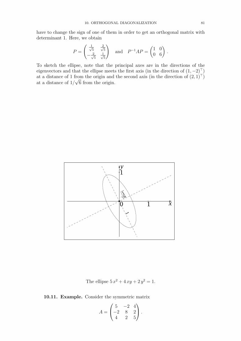
10. ORTHOGONAL DIAGONALIZATION 81
have to change the sign of one of them in order to get an orthogonal matrix withdeterminant 1. Here, we obtain
P =
(1√5
2√5
− 2√5
1√5
)and P−1AP =
(1 00 6
).
To sketch the ellipse, note that the principal axes are in the directions of theeigenvectors and that the ellipse meets the first axis (in the direction of (1,−2)>)at a distance of 1 from the origin and the second axis (in the direction of (2, 1)>)at a distance of 1/
√6 from the origin.
x
y
0 1
1
1
61
The ellipse 5x2 + 4xy + 2 y2 = 1.
10.11. Example. Consider the symmetric matrix
A =
5 −2 4−2 8 24 2 5
.

82 CONTENTS
We will determine an orthogonal matrix Q and a diagonal matrix D such thatA = QDQ>. The characteristic polynomial of A is the determinant of
tI − A =
t− 5 2 −42 t− 8 −2−4 −2 t− 5
,
which is easily determined to be PA(t) = t(t−9)2, so we have eigenvalues 0 and 9.The eigenspace for eigenvalue λ = 0 is the kernel kerA. From a row echelonform for A, which we will leave out here, we find that this kernel is generated by(2, 1,−2). Normalising gives the unit vector v1 = 1
3(2, 1,−2), which forms a basis
for the eigenspace for λ = 0. The eigenspace for eigenvalue λ = 9 is the kernel of
A− 9I =
−4 −2 4−2 −1 24 2 −4
.
A row echelon form for this matrix is2 1 −20 0 00 0 0
,
from which we find that this eigenspace is generated by w1 = (1, 0, 1) and w2 =(1,−2, 0). Within this eigenspace we apply Gram-Schmidt orthonormalisation tofind an orthonormal basis for the eigenspace. We find w1 and
w2 −〈w2, w1〉w1, w1
w1 = w2 − 12w1 = 1
2(1,−4,−1).
After normalising this yields v2 = 1√2(1, 0, 1) and v3 = 1
3√2(1,−4,−1).
Our new basis becomes B = (v1, v2, v3). By Lemma 10.2, the two eigenspaces areorthogonal to each other, so B is an orthonormal basis of eigenvectors. Hence, thematrix Q = [id]BE is orthogonal, that is, Q−1 = Q>. For the diagonal matrix
D = [fA]BB =
0 0 00 9 00 0 9
we find
A = [fA]EE = [id]BE · [fA]BB · [id]EB = QDQ−1 = QDQ>.
The matrix Q = [id]BE has the basis vectors of B as columns, so we have
Q =
23
1√2
13√2
13
0 −23
√2
−23
1√2− 1
3√2
.
Exercises.
(1) Suppose that A is a symmetric 2 × 2 matrix of determinant 2 for which(1−2
)is an eigenvector with eigenvalue −1.
(a) What is the other eigenvalue of A?(b) What is the other eigenspace?(c) Determine A.
(2) Consider the quadratic form q(x, y) = 11x2 − 16xy − y2.

11. EXTERNAL DIRECT SUMS 83
(a) Find a symmetric matrix A for which
q(x, y) = (x y) · A ·(xy
).
(b) Find real numbers a, b and an orthogonal map f : R2 → R2 so thatq(f(u, v)) = au2 + bv2 for all u, v ∈ R.
(c) What values does q(x, y) assume on the unit circle x2 + y2 = 1?(3) What values does the quadratic form q(x, y, z) = 2xy+2xz+y2−2yz+z2
assume when (x, y, z) ranges over the unit sphere x2 + y2 + z2 = 1 in R3?(4) Suppose that A is an anti-symmetric n×n matrix over the real numbers.
(a) Show that every eigenvalue of A over the complex numbers lies iniR.
(b) If n is odd, show that 0 is an eigenvalue of A.
11. External Direct Sums
Earlier in this course, we have discussed direct sums of linear subspaces of a vectorspace. In this section, we discuss a way to contruct a vector space out of a givenfamily of vector spaces in such a way that the given spaces can be identified withlinear subspaces of the new space, which becomes their direct sum.
11.1. Definition. Let F be a field, and let (Vi)i∈I be a family of F -vectorspaces. The (external) direct sum of the spaces Vi is the vector space
V =⊕i∈I
Vi ={
(vi) ∈∏i∈I
Vi : vi = 0 for all but finitely many i ∈ I}.
Addition and scalar multiplication in V are defined component-wise.
If I is finite, say I = {1, 2, . . . , n}, then we also write
V = V1 ⊕ V2 ⊕ · · · ⊕ Vn ;
as a set, it is just the cartesian product V1 × · · · × Vn.
11.2. Proposition. Let (Vi)i∈I be a family of F -vector spaces, and V =⊕i∈I⊕
Vj their direct sum.
(1) There are injective linear maps ιj : Vj → V given by
ιj(vj) = (0, . . . , 0, vj, 0, . . . ) with vj in the jth position
such that with Vj = ιj(Vj), we have V =⊕
j∈I Vj as a direct sum ofsubspaces.
(2) If Bj is a bais of Vj, then B =⋃j∈I ιj(Bj) is a basis of V.
(3) If W is another F -vector space, and φj : Vj → W are linear maps, thenthere is a unique linear map φ : V → W such that φj = φ ◦ ιj for allj ∈ I.
Proof.
(1) This is clear from the definitions, compare 2.2.
(2) This is again clear from 2.2.
(3) A linear map is uniquely determined by its values on a basis. Let B be abasis as in (2). The only way to get φj = φ◦ιj is to define φ(ιj(b)) = φj(b)for all b ∈ Bj; this gives a unique linear map φ : V → W .

84 CONTENTS
�
Statement (3) above is called the universal property of the direct sum. It is essen-tially the only thing we have to know about
⊕i∈I Vi; the explicit construction is
not really relevant (except to show that such an object exists).
12. The Tensor Product
As direct sums allow us to “add” vector spaces in a way (which corresponds to“adding” their bases by taking the disjoint union), the tensor product allows us to“multiply” vector spaces (“multiplying” their bases by taking a cartesian product).The main purpose of the tensor product is to “linearize” multilinear maps.
You may have heard of “tensors”. They are used in physics (there is, for example,the “stress tensor” or the “moment of inertia tensor”) and also in differentialgeometry (the “curvature tensor” or the “metric tensor”). Basically a tensor isan element of a tensor product (of vector spaces), like a vector is an element ofa vector space. You have seen special cases of tensors already. To start with, ascalar (element of the base field F ) or a vector or a linear form are trivial examplesof tensors. More interesting examples are given by linear maps, endomorphisms,bilinear forms and multilinear maps in general.
The vector space of m×n matrices over F can be identified in a natural way withthe tensor product (F n)∗⊗Fm. This identification corresponds to the interpreta-tion of matrices as linear maps from F n to Fm. The vector space of m×n matricesover F can also identified in a (different) natural way with (Fm)∗ ⊗ (F n)∗; thiscorresponds to the interpretation of matrices as bilinear forms on Fm × F n.
In these examples, we see that (for example), the set of all bilinear forms has thestructure of a vector space. The tensor product generalizes this. Given two vectorspaces V1 and V2, it produces a new vector space V1 ⊗ V2 such that we have anatural identification
Bil(V1 × V2,W ) ∼= Hom(V1 ⊗ V2,W )
for all vector spaces W . Here Bil(V1 × V2,W ) denotes the vector space of bilinearmaps from V1 × V2 to W . The following definition states the property we wantmore precisely.
12.1. Definition. Let V1 and V2 be two vector spaces. A tensor product ofV1 and V2 is a vector space V , together with a bilinear map φ : V1 × V2 → V ,satisfying the following “universal property”:
For every vector space W and bilinear map ψ : V1 × V2 → W , there is a uniquelinear map f : V → W such that ψ = f ◦ φ.
V1 × V2φ
//
ψ $$
V
f~~
W
In other words, the canonical linear map
Hom(V,W ) −→ Bil(V1 × V2,W ) , f 7−→ f ◦ φis an isomorphism.
It is easy to see that there can be at most one tensor product in a very specificsense.

12. THE TENSOR PRODUCT 85
12.2. Lemma. Any two tensor products (V, φ), (V ′, φ′) are uniquely isomor-phic in the following sense: There is a unique isomorphism ι : V → V ′ such thatφ′ = ι ◦ φ.
V
ι
��
V1 × V2
φ::
φ′ ##V ′
Proof. Since φ′ : V1×V2 → V ′ is a bilinear map, there is a unique linear mapι : V → V ′ making the diagram above commute. For the same reason, there is aunique linear map ι′ : V ′ → V such that φ = ι′ ◦ φ′. Now ι′ ◦ ι : V → V is a linearmap satisfying (ι′ ◦ ι) ◦ φ = φ, and idV is another such map. But by the universalproperty, there is a unique such map, hence ι′ ◦ ι = idV . In the same way, we seethat ι ◦ ι′ = idV ′ , therefore ι is an isomorphism. �
Beacuse of this uniqueness, it is allowable to simply speak of “the” tensor productof V1 and V2 (provided it exists! — but see below). The tensor product is denotedV1 ⊗ V2, and the bilinear map φ is written (v1, v2) 7→ v1 ⊗ v2.
It remains to show existence of the tensor product.
12.3. Proposition. Let V1 and V2 be two vector spaces; choose bases B1 of V1and B2 of V2. Let V be the vector space with basis B = B1 × B2, and define abilinear map φ : V1 × V2 → V via φ(b1, b2) = (b1, b2) ∈ B for b1 ∈ B1, b2 ∈ B2.Then (V, φ) is a tensor product of V1 and V2.
Proof. Let ψ : V1 × V2 → W be a bilinear map. We have to show that thereis a unique linear map f : V → W such that ψ = f ◦ φ. Now if this relation is tobe satisfied, we need to have f((b1, b2)) = f(φ(b1, b2)) = ψ(b1, b2). This fixes thevalues of f on the basis B, hence there can be at most one such linear map. Itremains to show that the linear map thus defined satisfies f(φ(v1, v2)) = ψ(v1, v2)for all v1 ∈ V1, v2 ∈ V2. But this is clear since ψ and f ◦ φ are two bilinear mapsthat agree on pairs of basis elements. �
12.4. Remark. This existence proof does not use that the bases are finiteand so also works for infinite-dimensional vector spaces (given the fact that everyvector space has a basis).
There is also a different construction that does not require the choice of bases. Theprice one has to pay is that one first needs to construct a gigantically huge space V(with basis V1×V2), which one then divides by another huge space (incorporatingall relations needed to make the map V1 × V2 → V bilinear) to end up with therelatively small space V1 ⊗ V2. This is a kind of “brute force” approach, but itworks.
Note that by the uniqueness lemma above, we always get “the same” tensor prod-uct, no matter which bases we choose.

86 CONTENTS
12.5. Elements of V1⊗V2. What do the elements of V1⊗V2 look like? Someof them are values of the bilinear map φ : V1 × V2 → V1 ⊗ V2, so are of the formv1 ⊗ v2. But these are not all! However, elements of this form span V1 ⊗ V2, andsince
λ(v1 ⊗ v2) = (λv1)⊗ v2 = v1 ⊗ (λv2)
(this comes from the bilinearity of φ), every element of V1 ⊗ V2 can be written asa (finite) sum of elements of the form v1 ⊗ v2.
The following result gives a more precise formulation that is sometimes useful.
12.6. Lemma. Let V and W be two vector spaces, and let w1, . . . , wn be abasis of W. Then every element of V ⊗W can be written uniquely in the form
n∑i=1
vi ⊗ wi = v1 ⊗ w1 + · · ·+ vn ⊗ wn
with v1, . . . , vn ∈ V.
Proof. Let x ∈ V ⊗W ; then by the discussion above, we can write
x = y1 ⊗ z1 + · · ·+ ym ⊗ zm
for some y1, . . . , ym ∈ V and z1, . . . , zm ∈ W. Since w1, . . . , wn is a basis of W, wecan write
zj = αj1w1 + · · ·+ αjnwn
with scalars αjk. Using the bilinearity of the map (y, z) 7→ y ⊗ z, we find that
x = y1 ⊗ (α11w1 + · · ·+ α1nwn) + · · ·+ ym ⊗ (αm1w1 + · · ·+ αmnwn)
= (α11y1 + · · ·+ αm1ym)⊗ w1 + · · ·+ (α1ny1 + · · ·+ αmnym)⊗ wn ,
which is of the required form.
For uniqueness, it suffices to show that
v1 ⊗ w1 + · · ·+ vn ⊗ wn = 0 =⇒ v1 = · · · = vn = 0 .
Assume that vj 6= 0. There is a bilinear form ψ on V ×W such that ψ(vj, wj) = 1and ψ(v, wi) = 0 for all v ∈ V and i 6= j. By the universal property of the tensorproduct, there is a linear form f on V ⊗W such that f(v⊗w) = ψ(v, w). Applyingf to both sides of the equation, we find that
0 = f(0) = f(v1 ⊗ w1 + · · ·+ vn ⊗ wn) = ψ(v1, w1) + · · ·+ ψ(vn, wn) = 1 ,
a contradiction. �
In this context, one can think of V ⊗W as being “the vector space W with scalarsreplaced by elements of V .” This point of view will be useful when we want toenlarge the base field, e.g., in order to turn a real vector space into a complexvector space of the same dimension.

12. THE TENSOR PRODUCT 87
12.7. Basic Properties of the Tensor Product. Recall the axioms satis-fied by a commutative “semiring” like the natural numbers:
a+ (b+ c) = (a+ b) + c
a+ b = b+ a
a+ 0 = a
a · (b · c) = (a · b) · ca · b = b · aa · 1 = a
a · (b+ c) = a · b+ a · c
(The name “semi”ring refers to the fact that we do not require the existence ofadditive inverses.)
All of these properties have their analogues for vector spaces, replacing additionby direct sum, zero by the zero space, multiplication by tensor product, one bythe one-dimensional space F , and equality by natural isomorphism:
U ⊕ (V ⊕W ) ∼= (U ⊕ V )⊕WU ⊕ V ∼= V ⊕ UU ⊕ 0 ∼= U
U ⊗ (V ⊗W ) ∼= (U ⊗ V )⊗WU ⊗ V ∼= V ⊗ UU ⊗ F ∼= U
U ⊗ (V ⊕W ) ∼= U ⊗ V ⊕ U ⊗W
There is a kind of “commutative diagram”:
(Finite Sets,∐,×,∼=)B 7→ #B
//
B 7→ FB++
(N,+, ·,=)
(Finite-dim. Vector Spaces,⊕,⊗,∼=)
dim
44
Let us prove some of the properties listed above.
Proof. We show that U ⊗ V ∼= V ⊗ U . We have to exhibit an isomorphism,or equivalently, linear maps going both ways that are inverses of each other. Bythe universal property, a linear map from U ⊗ V into any other vector space Wis “the same” as a bilinear map from U × V into W . So we get a linear mapf : U⊗V → V ⊗U from the bilinear map U×V → V ⊗U that sends (u, v) to v⊗u.So we have f(u⊗ v) = v ⊗ u. Similarly, there is a linear map g : V ⊗ U → U ⊗ Vthat satisfies g(v ⊗ u) = u ⊗ v. Since f and g are visibly inverses of each other,they are isomorphisms. �
Before we go on to the next statement, let us make a note of the principle we haveused.
12.8. Note. To give a linear map f : U ⊗ V → W, it is enough to specifyf(u ⊗ v) for u ∈ U , v ∈ V . The map U × V → W , (u, v) 7→ f(u ⊗ v) must bebilinear.

88 CONTENTS
Proof. We now show that U⊗(V ⊗W ) ∼= (U⊗V )⊗W . First fix u ∈ U . Thenby the principle above, there is a linear map fu : V ⊗W → (U⊗V )⊗W such thatfu(v⊗w) = (u⊗v)⊗w. Now the map U×(V ⊗W )→ (U⊗V )⊗W that sends (u, x)to fu(x) is bilinear (check!), so we get a linear map f : U⊗(V ⊗W )→ (U⊗V )⊗Wsuch that f(u⊗ (v ⊗ w)) = (u⊗ v)⊗ w. Similarly, there is a linear map g in theother direction such that g((u⊗ v)⊗w) = u⊗ (v⊗w). Since f and g are inversesof each other (this needs only be checked on elements of the form u⊗ (v ⊗ w) or(u⊗ v)⊗ w, since these span the spaces), they are isomorphisms. �
We leave the remaining two statements involving tensor products for the exercises.
Now let us look into the interplay of tensor products with linear maps.
12.9. Definition. Let f : V → W and f ′ : V ′ → W ′ be linear maps. ThenV × V ′ → W ⊗W ′, (v, v′) 7→ f(v) ⊗ f ′(v′) is bilinear and therefore correspondsto a linear map V ⊗ V ′ → W ⊗W ′, which we denote by f ⊗ f ′. I.e., we have
(f ⊗ f ′)(v ⊗ v′) = f(v)⊗ f ′(v′) .
12.10. Lemma. idV ⊗ idW = idV⊗W .
Proof. Obvious (check equality on elements v ⊗ w). �
12.11. Lemma. Let Uf−→ V
g−→ W and U ′f ′−→ V ′
g′−→ W ′ be linear maps.Then
(g ⊗ g′) ◦ (f ⊗ f ′) = (g ◦ f)⊗ (g′ ◦ f ′) .
Proof. Easy — check equality on u⊗ u′. �
12.12. Lemma. Hom(U,Hom(V,W )) ∼= Hom(U ⊗ V,W ).
Proof. Let f ∈ Hom(U,Hom(V,W )) and define f(u ⊗ v) =(f(u)
)(v) (note
that f(u) ∈ Hom(V,W ) is a linear map from V to W ). Since(f(u)
)(v) is bilinear
in u and v, this defines a linear map f ∈ Hom(U ⊗ V,W ). Conversely, givenϕ ∈ Hom(U ⊗ V,W ), define ϕ(u) ∈ Hom(V,W ) by
(ϕ(u)
)(v) = ϕ(u ⊗ v). Then
ϕ is a linear map from U to Hom(V,W ), and the two linear(!) maps f 7→ f andϕ 7→ ϕ are inverses of each other. �
In the special case W = F , the statement of the lemma reads
Hom(U, V ∗) ∼= Hom(U ⊗ V, F ) = (U ⊗ V )∗ .
The following result is important, as it allows us to replace Hom spaces by tensorproducts (at least when the vector spaces involved are finite-dimensional).

12. THE TENSOR PRODUCT 89
12.13. Proposition. Let V and W be two vector spaces. There is a naturallinear map
φ : V ∗ ⊗W −→ Hom(V,W ) , l ⊗ w 7−→(v 7→ l(v)w
),
which is an isomorphism when V or W is finite-dimensional.
Proof. We will give the proof here for the case that W is finite-dimensional,and leave the case “V finite-dimensional” for the exercises.
First we should check that φ is a well-defined linear map. By the general principleon maps from tensor products, we only need to check that (l, w) 7→
(v 7→ l(v)w
)is bilinear. Linearity in w is clear; linearity in l follows from the definition of thevector space structure on V ∗:
(α1l1 + α2l2, w) 7−→(v 7→ (α1l1 + α2l2)(v)w = α1l1(v)w + α2l2(v)w
)To show that φ is bijective when W is finite-dimensional, we choose a basisw1, . . . , wn of W . Let w∗1, . . . , w
∗n be the basis of W ∗ dual to w1, . . . , wn. Define a
map
φ′ : Hom(V,W ) −→ V ∗ ⊗W , f 7−→n∑i=1
(w∗i ◦ f)⊗ wi .
It is easy to see that φ′ is linear. Let us check that φ and φ′ are inverses. Recallthat for all w ∈ W , we have
w =n∑i=1
w∗i (w)wi .
Now,
φ′(φ(l ⊗ w)
)=
n∑i=1
(w∗i ◦ (v 7→ l(v)w)
)⊗ wi
=n∑i=1
(v 7→ l(v)w∗i (w))⊗ wi =n∑i=1
w∗i (w)l ⊗ wi
= l ⊗n∑i=1
w∗i (w)wi = l ⊗ w .
On the other hand,
φ(φ′(f)
)= φ
( n∑i=1
(w∗i ◦ f)⊗ wi)
=n∑i=1
(v 7→ w∗i
(f(v)
)wi
)=(v 7→
n∑i=1
w∗i (f(v))wi
)=(v 7→ f(v)
)= f .
�
Now assume that V = W is finite-dimensional. Then by the above,
Hom(V, V ) ∼= V ∗ ⊗ V
in a natural way. But Hom(V, V ) contains a special element, namely idV . Whatis the element of V ∗ ⊗ V that corresponds to it?

90 CONTENTS
12.14. Remark. Let v1, . . . , vn be a basis of V, and let v∗1, . . . , v∗n be the basis
of V ∗ dual to it. Then, with φ the canonical map from above, we have
φ( n∑i=1
v∗i ⊗ vi)
= idV .
Proof. Apply φ′ as defined above to idV . �
On the other hand, there is a natural bilinear form on V ∗×V , given by evaluation:(l, v) 7→ l(v). This gives the following.
12.15. Lemma. Let V be a finite-dimensional vector space. There is a linearform T : V ∗ ⊗ V → F given by T (l ⊗ v) = l(v). It makes the following diagramcommutative.
V ∗ ⊗ V φ//
T##
Hom(V, V )
Tryy
F
Proof. That T is well-defined is clear by the usual princpiple. (The vectorspace structure on V ∗ is defined in order to make evaluation bilinear!) We have tocheck that the diagram commutes. Fix a basis v1, . . . , vn, with dual basis v∗1, . . . , v
∗n,
and let f ∈ Hom(V, V ). Then φ−1(f) =∑
i(v∗i ◦ f) ⊗ vi, hence T (φ−1(f)) =∑
i v∗i (f(vi)). The terms in the sum are exactly the diagonal entries of the matrix A
representing f with respect to v1, . . . , vn, so T (φ−1(f)) = Tr(A) = Tr(f). �
The preceding operation is called “contraction”. More generally, it leads to linearmaps
U1 ⊗ · · · ⊗ Um ⊗ V ∗ ⊗ V ⊗W1 ⊗ · · · ⊗Wn −→ U1 ⊗ · · · ⊗ Um ⊗W1 · · · ⊗Wn .
This in turn is used to define “inner multiplication”
(U1 ⊗ · · · ⊗ Um ⊗ V ∗)× (V ⊗W1 ⊗ · · · ⊗Wn) −→ U1 ⊗ · · · ⊗ Um ⊗W1 · · · ⊗Wn
(by first going to the tensor product). The roles of V and V ∗ can also be reversed.This is opposed to “outer multiplication”, which is just the canonical bilinear map
(U1 ⊗ · · · ⊗ Um)× (W1 ⊗ · · · ⊗Wn) −→ U1 ⊗ · · · ⊗ Um ⊗W1 · · · ⊗Wn .
An important example of inner multiplication is composition of linear maps.
12.16. Lemma. Let U, V,W be vector spaces. Then the following diagramcommutes.
(l⊗v,l′⊗w)_
��
(U∗ ⊗ V )× (V ∗ ⊗W )
��
φ×φ// Hom(U, V )× Hom(V,W )
��
(f,g)_
��l′(v) l⊗w U∗ ⊗W φ
// Hom(U,W ) g◦f

12. THE TENSOR PRODUCT 91
Proof. We have
φ(l′ ⊗ w) ◦ φ(l ⊗ v) =(v′ 7→ l′(v′)w
)◦(u 7→ l(u)v
)=(u 7→ l′
(l(u)v
)w = l′(v)l(u)w
)= φ
(l′(v)l ⊗ w
).
�
12.17. Remark. Identifying Hom(Fm, F n) with the space Mat(n×m,F ) ofn×m-matrices over F , we see that matrix multiplication is a special case of innermultiplication of tensors.
12.18. Remark. Another example of inner multiplication is given by evalu-ation of linear maps: the following diagram commutes.
(l ⊗ w, v)_
��
(V ∗ ⊗W )× V φ×idV//
��
Hom(V,W )× V
��
(f, v)_
��
l(v)w W W f(v)
Complexification of Vector Spaces. Now let us turn to another use of thetensor product. There are situations when one has a real vector space, whichone would like to turn into a complex vector space with “the same” basis. Forexample, suppose that VR is a real vector space and WC is a complex vector space(writing the field as a subscript to make it clear what scalars we are considering),then W can also be considered as a real vector space (just by restricting the scalarmultiplication to R ⊂ C). We write WR for this space. Note that dimRWR =2 dimCWC — if b1, . . . , bn is a C-basis of W , then b1, ib1, . . . , bn, ibn is an R-basis.Now we can consider an R-linear map f : VR → WR. Can we construct a C-vectorspace VC out of V in such a way that f extends to a C-linear map f : VC → WC?(Of course, for this to make sense, VR has to sit in VR as a subspace.)
It turns out that we can use the tensor product to do this.
12.19. Lemma and Definition. Let V be a real vector space. The real vectorspace V = C⊗R V can be given the structure of a complex vector space by definingscalar multiplication as follows.
λ(α⊗ v) = (λα)⊗ v
V is embedded into V as a real subspace via ι : v 7→ 1⊗ v.
This C-vector space V is called the complexification of V .
Proof. We first have to check that the equation above leads to a well-definedR-bilinear map C× V → V . But this map is just
C× (C⊗R V ) −→ C⊗R (C⊗R V ) ∼= (C⊗R C)⊗R Vm⊗idV−→ C⊗R V ,
where m : C⊗RC→ C is induced from multiplication on C (which is certainly anR-bilinear map). Since the map is in particular linear in the second argument, wealso have the “distributive laws”
λ(x+ y) = λx+ λy , (λ+ µ)x = λx+ µx

92 CONTENTS
for λ, µ ∈ C, x, y ∈ V . The “associative law”
λ(µx) = (λµ)x
(for λ, µ ∈ C, x ∈ V ) then needs only to be checked for x = α ⊗ v, in which casewe have
λ(µ(α⊗ v)) = λ((µα)⊗ v) = (λµα)⊗ v = (λµ)(α⊗ v) .
The last statement is clear. �
If we apply the representation of elements in a tensor product given in Lemma 12.6to V , we obtain the following.
Suppose V has a basis v1, . . . , vn. Then every element of V can be written uniquelyin the form
α1 ⊗ v1 + · · ·+ αn ⊗ vn for some α1, . . . , αn ∈ C.
In this sense, we can consider V to have “the same” basis as V, but we allowcomplex coordinates instead of real ones.
On the other hand, we can consider the basis 1, i of C as a real vector space, thenwe see that every element of V can be written uniquely as
1⊗ v + i⊗ v′ = ι(v) + i · ι(v′) for some v, v′ ∈ V .
In this sense, elements of V have a real and an imaginary part, which live in V(identifying V with its image under ι in V ).
12.20. Proposition. Let V be a real vector space and W a complex vectorspace. Then for every R-linear map f : VR → WR, there is a unique C-linear mapf : VC → WC such that f ◦ ι = f (where ι : VR → VR is the map defined above).
V
f
��
V
ι
>>
f
W
Proof. The map C×V → W , (α, v) 7→ αf(v) is R-bilinear. By the universalproperty of the tensor product V = C ⊗R V , there is a unique R-linear mapf : V → W such that f(α⊗ v) = αf(v). Then we have
f(ι(v)) = f(1⊗ v) = f(v) .
We have to check that f is in fact C-linear. It is certainly additive (being R-linear),and for λ ∈ C, α⊗ v ∈ V ,
f(λ(α⊗ v)) = f((λα)⊗ v) = λαf(v) = λf(α⊗ v) .
Since any C-linear map f having the required property must be R-linear andsatisfy
f(α⊗ v) = f(α(1⊗ v)) = αf(1⊗ v) = αf(v) ,
and since there is only one such map, f is uniquely determined. �
13. SYMMETRIC AND ALTERNATING PRODUCTS 93
12.21. Remark. The proposition can be stated in the form that
HomR(V,W )∼=−→ HomC(V ,W ) , f 7−→ f ,
is an isomorphism. (The inverse is F 7→ F ◦ ι.)
We also get that R-linear maps between R-vector spaces give rise to C-linear mapsbetween their complexifications.
12.22. Lemma. Let f : V → W be an R-linear map between two R-vectorspaces. Then idC⊗f : V → W is C-linear, extends f , and is the only such map.
Proof. Consider the following diagram.
Vf//
ιV��
F
W
ιW��
VF
// W
Here, F = ιW ◦f is an R-linar map from V into the C-vector space W , hence thereis a unique C-linear map F : V → W such that the diagram is commutative. Weonly have to verify that F = idC⊗f . But
(idC⊗f)(α⊗ v) = α⊗ f(v) = α(1⊗ f(v)) = α(ιW ◦ f)(v) = αF (v) = F (α⊗ v) .
�
13. Symmetric and Alternating Products
Note. The material in this section is not required for the final exam.
Now we want to generalize the tensor product construction (in a sense) in orderto obtain similar results for symmetric and skew-symmetric (or alternating) bi-and multilinear maps.
13.1. Reminder. Let V and W be vector spaces. A bilinear map f : V ×V → W is called symmetric if f(v, v′) = f(v′, v) for all v, v′ ∈ V . f is calledalternating if f(v, v) = 0 for all v ∈ V ; this imples that f is skew-symmetric, i.e.,f(v, v′) = −f(v′, v) for all v, v′ ∈ V . The converse is true if the field of scalars isnot of characteristic 2.
Let us generalize these notions to multilinear maps.
13.2. Definition. Let V and W be vector spaces, and let f : V n → W be amultilinear map.
(1) f is called symmetric if
f(vσ(1), vσ(2), . . . , vσ(n)) = f(v1, v2, . . . , vn)
for all v1, . . . , vn ∈ V and all σ ∈ Sn.
The symmetric multilinear maps form a linear subspace of the space ofall multilinear maps V n → W , denoted Sym(V n,W ).

94 CONTENTS
(2) f is called alternating if
f(v1, v2, . . . , vn) = 0
for all v1, . . . , vn ∈ V such that vi = vj for some 1 ≤ i < j ≤ n.
The alternating multilinear maps form a linear subspace of the space ofall multilinear maps V n → W , denoted Alt(V n,W ).
13.3. Remark. Since transpositions generate the symmetric group Sn, wehave the following.
(1) f is symmetric if and only if it is a symmetric bilinear map in all pairs ofvariables, the other variables being fixed.
(2) f is alternating if and only if it is an alternating bilinear map in all pairsof variables, the other variables being fixed.
(3) Assume that the field of scalars has characteristic 6= 2. Then f is alter-nating if and only if
f(vσ(1), vσ(2), . . . , vσ(n)) = ε(σ)f(v1, v2, . . . , vn)
for all v1, . . . , vn ∈ V and all σ ∈ Sn, where ε(σ) is the sign of thepermutation σ.
13.4. Example. We know from earlier that the determinant can be inter-preted as an alternating multilinear map V n → F , where V is an n-dimensionalvector space — consider the n vectors in V as the n columns in a matrix. More-over, we had seen that up to scaling, the determinant is the only such map. Thismeans that
Alt(V n, F ) = F det .
13.5. We have seen that we can express multilinear maps as elements of suit-able tensor products: Assuming V and W to be finite-dimensional, a multilinearmap f : V n → W lives in
Hom(V ⊗n,W ) ∼= (V ∗)⊗n ⊗W .
Fixing a basis v1, . . . , vm of V and its dual basis v∗1, . . . , v∗n, any element of this
tensor product can be written uniquely in the form
f =m∑
i1,...,in=1
v∗i1 ⊗ · · · ⊗ v∗in ⊗ wi1,...,in
with suitable wi1...in ∈ W . How can we read off whether f is symmetric or alter-nating?
13.6. Definition. Let x ∈ V ⊗n.
(1) x is called symmetric if sσ(x) = x for all σ ∈ Sn, where sσ : V ⊗n → V ⊗n
is the automorphism given by
sσ(v1 ⊗ v2 ⊗ · · · ⊗ vn) = vσ(1) ⊗ vσ(2) ⊗ · · · ⊗ vσ(n) .
We will write Sym(V ⊗n) for the subspace of symmetric tensors.
(2) x is called skew-symmetric if sσ(x) = ε(σ)x for all σ ∈ Sn.We will write Alt(V ⊗n) for the subspace of skew-symmetric tensors.

13. SYMMETRIC AND ALTERNATING PRODUCTS 95
13.7. Proposition. Let f : V n → W be a multilinear map, indentified withits image in (V ∗)⊗n ⊗W . The following statements are equivalent.
(1) f is a symmetric multilinear map.
(2) f ∈ (V ∗)⊗n ⊗W lies in the subspace Sym((V ∗)⊗n)⊗W .
(3) Fixing a basis as above in 13.5, in the representation of f as given there,we have
wiσ(1),...,iσ(n) = wi1,...,in
for all σ ∈ Sn.
Note that in the case W = F and n = 2, the equivalence of (1) and (3) is just thewell-known fact that symmetric matrices encode symmetric bilinear forms.
Proof. Looking at (3), we have that wi1,...,in = f(vi1 , . . . , vin). So symmetryof f (statement (1)) certainly implies (3). Assuming (3), we see that f is a linearcombination of terms of the form(∑
σ∈Sn
vdiσ(1) ⊗ · · · ⊗ vdiσ(n)
)⊗ w
(with w = wi1,...,in), all of which are in the indicated subspace Sym((V ∗)⊗n)⊗Wof (V ∗)⊗n ⊗ W , proving (2). Finally, assuming (2), we can assume f = x ⊗ wwith x ∈ Sym((V ∗)⊗n) and w ∈ W . For y ∈ V ⊗n and z ∈ (V ∗)⊗n ∼= (V ⊗n)∗,we have (sσ(z))(sσ(y)) = z(y). Since sσ(x) = x, we get x(sσ(y)) = x(y) for allσ ∈ Sn, which implies that f(sσ(y)) = x(sσ(y)) ⊗ w = x(y) ⊗ w = f(y). So f issymmetric. �
13.8. Proposition. Let f : V n → W be a multilinear map, indentified withits image in (V ∗)⊗n ⊗W . The following statements are equivalent.
(1) f is an alternating multilinear map.
(2) f ∈ (V ∗)⊗n ⊗W lies in the subspace Alt((V ∗)⊗n)⊗W .
(3) Fixing a basis as above in 13.5, in the representation of f as given there,we have
wiσ(1),...,iσ(n) = ε(σ)wi1,...,in
for all σ ∈ Sn.
The proof is similar to the preceding one.
The equivalence of (2) and (3) in the propositions above, in the special case W = Fand replacing V ∗ by V , gives the following. (We assume that F is of characteristiczero, i.e., that Q ⊂ F .)
13.9. Proposition. Let V be an m-dimensional vector space with basis v1, . . . , vm.
(1) The elements ∑σ∈Sn
viσ(1) ⊗ · · · ⊗ viσ(n)
for 1 ≤ i1 ≤ i2 ≤ · · · ≤ in ≤ m form a basis of Sym(V ⊗n). In particular,
dim Sym(V ⊗n) =
(m+ n− 1
n
).

96 CONTENTS
(2) The elements ∑σ∈Sn
ε(σ)viσ(1) ⊗ · · · ⊗ viσ(n)
for 1 ≤ i1 < i2 < · · · < in ≤ m form a basis of Alt(V ⊗n). In particular,
dim Alt(V ⊗n) =
(m
n
).
Proof. It is clear that the given elements span the spaces. They are linearlyindependent since no two of them involve the same basis elements of V ⊗n. (In thealternating case, note that the element given above vanishes if two of the ij areequal.) �
The upshot of this is that (taking W = F for simplicity) we have identified
Sym(V n, F ) = Sym((V ∗)⊗n) ⊂ (V ∗)⊗n = (V ⊗n)∗
and
Alt(V n, F ) = Alt((V ∗)⊗n) ⊂ (V ∗)⊗n = (V ⊗n)∗
as subspaces of (V ⊗n)∗. But what we would like to have are spaces Symn(V ) andAltn(V ) such that we get identifications
Sym(V n, F ) = Hom(Symn(V ), F ) = (Symn(V ))∗
and
Alt(V n, F ) = Hom(Altn(V ), F ) = (Altn(V ))∗ .
Now there is a general principle that says that subspaces are “dual” to quotientspaces: If W is a subspace of V , then W ∗ is a quotient space of V ∗ in a naturalway, and if W is a quotient of V , then W ∗ is a subspace of V ∗ in a natural way. Soin order to translate the subspace Sym(V n, F ) (or Alt(V n, F )) of the dual spaceof V ⊗n into the dual space of something, we should look for a suitable quotientof V ⊗n!
13.10. Definition. Let V be a vector space, n > 0 an integer.
(1) Let W ⊂ V ⊗n be the subspace spanned by all elements of the form
v1 ⊗ v2 ⊗ · · · ⊗ vn − vσ(1) ⊗ vσ(2) ⊗ · · · ⊗ vσ(n)for v1, v2, . . . , vn ∈ V and σ ∈ Sn. Then the quotient space
Symn(V ) = Sn(V ) = V ⊗n/W
is called the nth symmetric tensor power of V . The image of v1 ⊗ v2 ⊗· · · ⊗ vn in Sn(V ) is denoted v1 · v2 · · · vn.
(2) Let W ⊂ V ⊗n be the subspace spanned by all elements of the form
v1 ⊗ v2 ⊗ · · · ⊗ vnfor v1, v2, . . . , vn ∈ V such that vi = vj for some 1 ≤ i < j ≤ n. Then thequotient space
Altn(V ) =∧n(V ) = V ⊗n/W
is called the nth alternating tensor power of V . The image of v1 ⊗ v2 ⊗· · · ⊗ vn in
∧n(V ) is denoted v1 ∧ v2 ∧ · · · ∧ vn.

13. SYMMETRIC AND ALTERNATING PRODUCTS 97
13.11. Theorem.
(1) The map
ϕ : V n −→ Sn(V ) , (v1, v2, . . . , vn) 7−→ v1 · v2 · · · vnis multilinear and symmetric. For every multilinear and symmetric mapf : V n → U , there is a unique linear map g : Sn(V ) → U such thatf = g ◦ ϕ.
(2) The map
ψ : V n −→∧n(V ) , (v1, v2, . . . , vn) 7−→ v1 ∧ v2 ∧ · · · ∧ vn
is multilinear and alternating. For every multilinear and alternating mapf : V n → U , there is a unique linear map g :
∧n(V ) → U such thatf = g ◦ ψ.
These statements tell us that the spaces we have defined do what we want: Weget identifications
Sym(V n, U) = Hom(Sn(V ), U) and Alt(V n, U) = Hom(∧n(V ), U) .
Proof. We prove the first part; the proof of the second part is analogous.First, it is clear that ϕ is multilinear: it is the composition of the multilinear map(v1, . . . , vn) 7→ v1 ⊗ · · · ⊗ vn and the linear projection map from V ⊗n to Sn(V ).We have to check that ϕ is symmetric. But
ϕ(vσ(1), . . . , vσ(n))− ϕ(v1, . . . , vn) = vσ(1) · · · vσ(n) − v1 · · · vn = 0 ,
since it is the image in Sn(V ) of vσ(1) ⊗ · · · ⊗ vσ(n) − v1 ⊗ · · · ⊗ vn ∈ W . Now letf : V n → U be multilinear and symmetric. Then there is a unique linear mapf ′ : V ⊗n → U corresponding to f , and by symmetry of f , we have
f ′(vσ(1) ⊗ · · · ⊗ vσ(n) − v1 ⊗ · · · ⊗ vn) = 0 .
So f ′ vanishes on all the elements of a spanning set of W . Hence it vanishes on Wand therefore induces a unique linear map g : Sn(V ) = V ⊗n/W → U .
V n
f""
//
ϕ
))
V ⊗n
f ′
��
// // Sn(V )
gzz
U
�
The two spaces Sym(V ⊗n) and Sn(V ) (resp., Alt(V ⊗n) and∧n(V )) are closely
related. We assume that F is of characteristic zero.
13.12. Proposition.
(1) The maps Sym(V ⊗n) ⊂ V ⊗n → Sn(V ) and
Sn(V ) −→ Sym(V ⊗n) , v1 · v2 · · · vn 7−→1
n!
∑σ∈Sn
vσ(1) ⊗ vσ(2) ⊗ · · · ⊗ vσ(n)
are inverse isomorphisms. In particular, if b1, . . . , bm is a basis of V , thenthe elements
bi1 · bi2 · · · bin with 1 ≤ i1 ≤ i2 ≤ · · · ≤ in ≤ m
form a basis of Sn(V ), and dimSn(V ) =(m+n−1
n
).

98 CONTENTS
(2) The maps Alt(V ⊗n) ⊂ V ⊗n →∧n(V ) and∧n(V ) −→ Alt(V ⊗n) , v1∧v2∧· · ·∧vn 7−→
1
n!
∑σ∈Sn
sign(σ)vσ(1)⊗vσ(2)⊗· · ·⊗vσ(n)
are inverse isomorphisms. In particular, if b1, . . . , bm is a basis of V , thenthe elements
bi1 ∧ bi2 ∧ · · · ∧ bin with 1 ≤ i1 < i2 < · · · < in ≤ m
form a basis of∧n(V ), and dim
∧n(V ) =(mn
).
Proof. It is easy to check that the specified maps are well-defined linear mapsand inverses of each other, so they are isomorphisms. The other statements thenfollow from the description in Prop. 13.9. �
Note that if dimV = n, then we have∧n(V ) = F (v1 ∧ · · · ∧ vn)
for any basis v1, . . . , vn of V .
13.13. Corollary. Let v1, . . . , vn ∈ V . Then v1, . . . , vn are linearly indepen-dent if and only if v1 ∧ · · · ∧ vn 6= 0.
Proof. If v1, . . . , vn are linearly dependent, then we can express one of them,say vn, as a linear combination of the others:
vn = λ1v1 + · · ·+ λn−1vn−1 .
Then
v1 ∧ · · · ∧ vn−1 ∧ vn = v1 ∧ · · · ∧ vn−1 ∧ (λ1v1 + · · ·+ λn−1vn−1)
= λ1(v1 ∧ · · · ∧ vn−1 ∧ v1) + · · ·+ λn−1(v1 ∧ · · · ∧ vn−1 ∧ vn−1)= 0 + · · ·+ 0 = 0 .
On the other hand, when v1, . . . , vn are linearly independent, they form part ofa basis v1, . . . , vn, . . . , vm, and by Prop. 13.12, v1 ∧ · · · ∧ vn is a basis element of∧n(V ), hence nonzero. �
13.14. Lemma and Definition. Let f : V → W be linear. Then f induceslinear maps Sn(f) : Sn(V )→ Sn(W ) and
∧n(f) :∧n(V )→
∧n(W ) satisfying
Sn(f)(v1 · · · vn) = f(v1) · · · f(vn) ,∧n(f)(v1 ∧ · · · ∧ vn) = f(v1) ∧ · · · ∧ f(vn) .
Proof. The map V n → Sn(W ), (v1, . . . , vn) 7→ f(v1) · · · f(vn), is a symmetricmultilinear map and therefore determines a unique linear map Sn(f) : Sn(V ) →Sn(W ) with the given property. Similarly for
∧n(f). �

13. SYMMETRIC AND ALTERNATING PRODUCTS 99
13.15. Proposition. Let f : V → V be a linear map, with V an n-dimensionalvector space. Then
∧n(f) :∧n(V )→
∧n(V ) is multiplication by det(f).
Proof. Since∧n(V ) is a one-dimensional vector space,
∧n(f) must be multi-plication by a scalar. We pick a basis v1, . . . , vn of V and represent f by a matrix Awith respect to this basis. The scalar in question is the element δ ∈ F such that
f(v1) ∧ f(v2) ∧ · · · ∧ f(vn) = δ (v1 ∧ v2 ∧ · · · ∧ vn) .
The vectors f(v1), . . . , f(vn) correspond to the columns of the matrix A, and δ isan alternating multilinear form on them. Hence δ must be det(A), up to a scalarfactor. Taking f to be idV , we see that the scalar factor is 1. �
13.16. Corollary. Let V be a finite-dimensional vector space, f, g : V → Vtwo endomorphisms. Then det(g ◦ f) = deg(g) det(f).
Proof. Let n = dimV. We have∧n(g ◦f) =
∧n g ◦∧n f , and the map on the
left is multiplication by det(g ◦ f), whereas the map on the right is multiplicationby det(g) det(f). �
We see that, similarly to the trace Hom(V, V ) ∼= V ∗ ⊗ V → F , our constructionsgive us a natural (coordinate-free) definition of the determinant of an endomor-phism.


Bibliography
[BR1] T.S. Blyth and E.F. Robertson: Basic Linear Algebra. Springer UndergraduateMathematics Series, 2002.
[BR2] T.S. Blyth and E.F. Robertson: Further Linear Algebra. Springer UndergraduateMathematics Series, 2002.
[J] K. Janich: Linear Algebra. Springer Undergraduate Texts in Mathematics, 1994[KM] A. Kostrykin and Y. Manin: Linear Algebra and Geometry. Gordan and Breach,
1988.
101


Index of notation
Eλ(f), 2Pf , 2⊕
i∈I Ui, 4⊕, 4⊕
i∈I fi, 6fn, 7p(f), 7diag, 9Mf , 11B(m), 17B(λ,m), 26exp, 29B′(λ, µ,m), 30V ∗, 39(v∗1 , . . . , v
∗n), 39
V ∗∗, 41αV , 41evv, 41evα, 41f>, 42〈 , 〉, 42ϕn, 42P−>, 44S◦, 47‖ · ‖, 49‖ · ‖∞, 50‖ · ‖2, 50‖ · ‖1, 50d(·, ·), 50Bil(V,W ), 52Bil(V ), 52φL, 53φR, 53βV,W , 54〈·, ·〉, 65V , 66‖ · ‖, 66⊥, 66d(·, ·), 67f∗, 70A∗, 73⊕
i∈I Vi, 83⊕, 83ιj , 83ι, 85V1 ⊗ V2, 86v1 ⊗ v2, 86f ⊗ f ′, 88
V , 91f , 92Sym(V n,W ), 93Alt(V n,W ), 94Sym(V ⊗n), 94Alt(V ⊗n), 94Sn, 96v1 · v2, 96∧n
, 96v1 ∧ v2, 96Sn(f), 98∧n
(f), 98
103


Index
adjoint, 71image, 73kernel, 73matrix representation, 73properties, 71
algebraic multiplicity, 2algebraically closed, 12alternating bilinear form, 52, 57alternating bilinear map, 93alternating multilinear map, 93
equivalent statements, 95alternating tensor power, 96
basis, 97dimension, 97linear map, 98
nth alternating tensor power, 96annihilator, 47
dimension formula, 47Axiom of Choice, 4
basisdual, 39
basis changebilinear form, 55dual, 44
Bessel’s inequality, 69bidual, 40
relation to αV , 44bilinear form, 52
alternating, 52, 57basis change, 55isomorphism Bil(V,W )→ Hom(V,W ∗),
53matrix representation, 55nondegenerate, 53, 57rank, 62represents linear form, 54signature, 62skew-symmetric, 52, 57symmetric, 52, 57
can be diagonalized, 59classification, 59classification over C, 61classification over R, 61
bilinear map, 52alternating, 93skew-symmetric, 93symmetric, 93
block diagonal matrix, 6, 17
canonical map αVrelation to f>>, 44
canonical map αv, 40Cauchy-Schwarz inequality, 67Cayley-Hamilton Theorem, 10characteristic polynomial, 2classification of symmetric bilinear forms,
59classification of symmetric bilinear forms
over C, 61classification of symmetric bilinear forms
over R, 61complex conjugate space, 66complex inner product space, 65complexification, 91
linear map, 92congruent matrices, 56conic section, 80conjugate-linear, 65contraction, 90coordinate map, 39coprime polynomials, 7criterion for positive definiteness, 62
determinantis multiplicative, 99of direct sum, 6
diagonal part endomorphism, 27uniqueness, 31
diagonalizable, 2minimal polynomial, 12nilpotent matrix/endomorphism is zero,
14simultaneously, 30
diagonalize a matrix, 60differential equations
linear, first-order with constantcoefficients, 29
direct sumdeterminant, 6external, 83of endomorphisms, 5
relation to characteristic polynomial, 7relation to minimal polynomial, 7
of subspaces, 4orthogonal, 58
105

106 INDEX
trace, 6universal property, 84
distance, 67division of polynomials, 11dot product, 42dual
basis, 39uniqueness, 39
basis change, 44linear map, 42
inverse, 42matrix representation, 43
of canonical map αV , 44vector space, 39
dimension, 40
eigenspace, 2generalized, 26
λ-eigenspace, 2eigenvalue, 2eigenvector, 2endomorphism ring
is isomorphic to V ∗ ⊗ V , 89equivalent norms, 50euclidean norm, 50evaluation map, 41evaluation paring, 52exact, 46exponential
matrix, 29external direct sum, 83
Fourier expansion, 70
generalized eigenspace, 26geometric multiplicity, 2Gram-Schmidt Orthonormalization
Process, 68
Hermitian inner product, 65Hermitian matrix, 74Hilbert matrix, 56
ideal, 12inner multiplication, 90
composition, 90evaluation, 91
inner product, 65inner product space, 65
complex, 65real, 65
invariant subspace, 6f -invariant subspace, 6isometry, 71
characterization, 72
Jordan Normal Form, 26, 27general version, 29real, 29
kernel matrix, 46
Lagrange interpolation polynomials, 41left kernel, 53linear form, 39linear functional, 39
matrix exponential, 29matrix representation
adjoint, 73dual linear map, 43of bilinear forms, 55
maximum norm, 50metric, 50minimal polynomial, 11
of diagonalizable matrix/endomorphism,12
of nilpotent matrix/endomorphism, 14uniqueness, 11
minimum polynomial, see also minimalpolynomial, 11
multilinear mapalternating, 93
equivalent statements, 95symmetric, 93
equivalent statements, 94multiplicity
algebraic, 2geometric, 2
nilpotent, 14nilpotent matrix/endomorphism
characteristic polynomial, 17diagonalizable iff zero, 14minimal polynomial, 14structure of, 15, 17
nilpotent part endomorphism, 27uniqueness, 31
nondegenerate bilinear form, 53, 57norm, 49, 67
equivalent, 50is continuous, 50
normal, 71normal endomorphism
complex inner product spaceis orthodiagonalizable, 79
is self-adjoint iff all eigenvalues are real,79
properties, 77normal matrix, 74
ONB, 66orientation preserving, 80orthodiagonalizable, 77
criterion complex inner product space, 79criterion real inner product space, 79
orthogonal, 66subspace, 58
orthogonal complement, 59orthogonal direct sum, 58, 78orthogonal map, 75orthogonal matrix, 74

INDEX 107
orthogonal set, 66is linearly independent, 69
orthogonally diagonalized, 77orthogonally similar, 80orthonormal, 66orthonormal basis, 66
equivalent statements, 69orthonormal set, 66orthonormalization, 68outer multiplication, 90
Parseval’s identity, 70polynomial
characteristic, 2coprime, 7division (algorithm), 11minimal, 11
positive definite, 61positive definiteness
criterion, 62principal axes, 80
transformation, 80principal ideal domain, 12
quadric, 80
rank of a bilinear form, 62real inner product space, 65Real Jordan Normal Form, 29right kernel, 53
scalar product, 42self-adjoint, 71self-adjoint endomorphism
real inner product spaceis orthodiagonalizable, 79
semi-simple, 29semiring, 86semiring of vector spaces, 87sesquilinear form, 65signature of a bilinear form, 62simultaneously diagonalizable, 30skew-symmetric bilinear form, 52, 57skew-symmetric bilinear map, 93skew-symmetric tensor, 94Spectral Theorem, 79subspace of alternating tensors
dimension, 95subspace of symmetric tensors
dimension, 95sum norm, 50symmetric bilinear form, 52, 57
can be diagonalized, 59classification, 59classification over C, 61classification over R, 61
symmetric bilinear map, 93symmetric matrix, 74
is diagonalizable, 80symmetric multilinear map, 93
equivalent statements, 94
symmetric tensor, 94symmetric tensor power, 96
basis, 97dimension, 97linear map, 98
nth symmetric tensor power, 96
tensor product, 84elements, 86existence, 85linear map, 87, 88of finite dimensional vector spaces
is isomorphic to Hom(V,W ), 88uniqueness, 84
traceof direct sum, 6
transpose linear map, see also dual linearmap
triangle inequality, 49, 67
unit vector, 66unitary map, 75unitary matrix, 74
Vandermonde Matrix, 41
Zorn’s Lemma, 4, 41