Embed Size (px)
Citation preview
Chapter 4
Linear Algebra I, Theoryand Conditioning
61
62 CHAPTER 4. LINEAR ALGEBRA I, THEORY AND CONDITIONING
4.1 Introduction
Linear algebra and calculus are the basic tools of quantitative science. The oper-ations of linear algebra include solving systems of equations, finding subspaces,solving least squares problems, factoring matrices, and computing eigenvaluesand eigenvectors. In practice most of these operations will be done by soft-ware packages that you buy or download. This chapter discusses formulationand condition number of the main problems in computational linear algebra.Chapter 5.1 discusses algorithms.
Conditioning is the primary concern in many practical linear algebra com-putations. Easily available linear algebra software is stable in the sense thatthe results are as accurate as the conditioning of the problem allows. Unfor-tunately, condition numbers as large as 1018 occur in not terribly large or rarepractical problems. The results of such a calculation in double precision wouldbe completely unreliable.
If a computational method for a well conditioned problem is unstable (muchless accurate than its conditioning allows), it is likely because one of the sub-problems is ill conditioned. For example, the problem of computing the matrixexponential, eA, may be well conditioned while the problem of computing theeigenvalues and eigenvectors of A is ill conditioned. A stable algorithm for com-puting eA in that case must avoid using the eigenvalues and eigenvectors of A,see Exercise 12.
The condition number measures how small perturbations in the data affectthe answer. This is called perturbation theory in linear algebra. Suppose1 A is amatrix and f(A) is the solution of a linear algebra problem involving A, such asx that satisfies Ax = b, or λ and v that satisfies Av = λv. Perturbation theoryseeks to estimate ∆f = f(A + ∆A) − f(A) when ∆A is small. Usually, thisamounts to calculating the derivative of f with respect to A. We often do thisby applying implicit differentiation to the relevant equations (such as Ax = b).
It often is helpful to simplify the results of perturbation calculations usingsimple bounds that involve vector or matrix norms. For example, suppose wewant to say that all the entries in ∆A or ∆v are small. For a vector, v, or amatrix, A, the norm, ‖v‖ or ‖A‖, is a number that characterizes the size of vor A. Using norms, we can say that the relative size of a perturbation in A is‖∆A‖ / ‖A‖.
The condition number of a problem involving A depends on the problem aswell as on A. For example, the condition number of f(A) = A−1b, the problemof finding x so that Ax = b, informally2 is given by
∥∥A∥∥∥∥A−1
∥∥ . (4.1)
The problem of finding the eigenvectors of A has a condition number that does
1This notation replaces our earlier A(x). In linear algebra, A always is a matrix and xnever is a matrix.
2To get this result, we not only maximize over ∆A but also over b. If the relative error
really were increased by a factor on the order of ‖A‖∥∥A−1
∥∥ the finite element method, which
is the main computational technique for structural analysis, would not work.
4.1. INTRODUCTION 63
not resemble (4.1). For example, finding eigenvectors of A can be well condi-tioned even when
∥∥A−1∥∥ is infinite (A is singular).
There are several ways to represent an n × n matrix in the computer. Thesimplest is to store the n2 numbers in an n × n array. If this direct storage isefficient, we say A is dense. Much of the discussion here and in Chapter 5.1applies mainly to dense matrices. A matrix is sparse if storing all its entriesdirectly is inefficient. A modern (2006) desktop computer has enough memoryfor n2 numbers if if n is less than about3 50, 000. This makes dense matrixmethods impractical for solving systems of equations with more than 50, 000variables. The computing time solving n = 50, 000 linear equations in this waywould be about a day. Sparse matrix methods can handle larger problems andoften give faster methods even for problems that can be handled using densematrix methods. For example, finite element computations often lead to sparsematrices with orders of magnitude larger n that can be solved in minutes
One way a matrix can be sparse is for most of its entries to be zero. Forexample, discretizations of the Laplace equation in three dimensions have asfew as seven non-zero entries per row, so that 7/n is the fraction of entries of Athat are not zero. Sparse matrices in this sense also arise in circuit problems,where a non-zero entry in A corresponds to a direct connection between twoelements in the circuit. Such matrices may be stored in sparse matrix format,in which we keep lists noting which entries are not zero and the values of thenon-zero elements. Computations with such sparse matrices try to avoid fill in.For example, they would avoid explicit computation of A−1 because most of itsentries are not zero. Sparse matrix software has heuristics that often do verywell in avoiding fill in. The interested reader should consult the references.
In some cases it is possible to compute the matrix vector product y = Ax fora given x efficiently without calculating the entries of A explicitly. One exampleis the discrete Fourier transform (DFT) described in Chapter 1. This is a fullmatrix (every entry different from zero) with n2 non-zero entries, but the FFT(fast Fourier transform) algorithm computes y = Ax in O(n log(n)) operations.Another example is the fast multipole method that computes forces from mutualelectrostatic interaction of n charged particles with b bits of accuracy in O(nb)work. Many finite element packages never assemble the stiffness matrix, A.
Computational methods can be direct or iterative. A direct method would getthe exact answer in exact arithmetic using a predetermined number of arithmeticoperations. For example, Gauss elimination computes the LU factorization of Ausing O(n3) operations. Iterative methods produce a sequence of approximatesolutions that converge to the exact answer as the number of iterations goes toinfinity. They usually are faster than direct methods for very large problems,particularly when A is sparse.
3With n2 floating point numbers and 8 bytes per number (double precision), we need50, 0002 × 8 = 2 · 1010 bytes, which is 20GBytes.
64 CHAPTER 4. LINEAR ALGEBRA I, THEORY AND CONDITIONING
4.2 Review of linear algebra
This section recalls some aspects of linear algebra we make use of later. It is nota substitute for a course on linear algebra. We make use of many things fromlinear algebra, such as matrix inverses, without explanation. People come toscientific computing with vastly differing points of view in linear algebra. Thissection should give everyone a common language.
4.2.1 Vector spaces
Linear algebra gets much of its power through the interaction between the ab-stract and the concrete. Abstract linear transformations are represented byconcrete arrays of numbers forming a matrix. The set of solutions of a homo-geneous system of equations forms an abstract subspace of Rn that we can tryto characterize. For example, a basis for such a subspace may be computed byfactoring a matrix in a certain way.
A vector space is a set of elements that may be added and multiplied byscalar numbers4 (either real or complex numbers, depending on the application).Vector addition is commutative (u + v = v + u) and associative ((u + v) + w =u + (v + w)). Multiplication by scalars is distributive over vector addition(a(u + v) = au + av and (a + b)u = au + bu for scalars a and b and vectors uand v). There is a unique zero vector, 0, with 0 + u = u for any vector u.
The standard vector spaces are Rn (or Cn), consisting of column vectors
u =
u1
u2
··
un
where the components, uk, are arbitrary real (or complex) numbers. Vectoraddition and scalar multiplication are done componentwise.
If V is a vector space and V ′ ⊂ V , then we say that V ′ is a subspace of V ifV ′ is also a vector space with the same vector addition and scalar multiplicationoperations. We may always add elements of V ′ and multiply them by scalars,but V ′ is a subspace if the result always is an element of V ′. We say V ′ isa subspace if it is closed under vector addition and scalar multiplication. Forexample, suppose V = Rn and V ′ consists of all vectors whose components sumto zero (
∑nk=1 uk = 0). If we add two such vectors or multiply by a scalar, the
result also has the zero sum property. On the other hand, the set of vectorswhose components sum to one (
∑nk=1 uk = 1) is not closed under vector addition
or scalar multiplication.
4Physicists use the word “scalar” in a different way. For them, a scalar is a number thatis the same in any coordinate system. The components of a vector in a particular basis arenot scalars in this sense.
4.2. REVIEW OF LINEAR ALGEBRA 65
A basis for vector space V is a set of vectors f1, . . ., fn so that any u ∈ Vmay be written in a unique way as a linear combination of the vectors fk:
u = u1f1 + · · ·+ unfn ,
with scalar expansion coefficients uk. The standard vector spaces Rn and Cn
have standard bases ek, the vector with all zero components but for a single 1in position k. This is a basis because
u =
u1
u2
··
un
= u1
10··0
+ u2
01··0
+ · · ·+ un
00··1
=
n∑
k=1
ukek .
In view of this, there is little distinction between coordinates, components, andexpansion coefficients, all of which are called uk. If V has a basis with n ele-ments, we say the dimension of V is n. It is possible to make this definitionbecause of the theorem that states that every basis of V has the same numberof elements. A vector space that does not have a finite basis is called infinite di-mensional5. The vector space of all polynomials (with no limit on their degree)is infinite dimensional.
Polynomials provide other examples of vector spaces. A polynomial in thevariable x is a linear combination of powers of x, such as 2 + 3x4, or 1, or13 (x − 1)2(x3 − 3x)6. We could multiply out the last example to write it as alinear combination of powers of x. The degree of a polynomial is the highestpower that it contains. The complicated product above has degree 20. Onevector space is the set, Pd, of all polynomials of degree not more than d. Thisspace has a basis consisting of d + 1 elements:
f0 = 1 , f1 = x , . . . , fd = xd .
Another basis of P3 consists of the “Hermite” polynomials
H0 = 1 , H1 = x , H2 = x2 − 1 , H3 = x3 − 3x .
These are useful in probability because if x is a standard normal random vari-able, then they are uncorrelated:
E [Hj(X)Hk(X)] =1√2π
∫ ∞
−∞Hj(x)Hk(x)e−x2/2dx = 0 if j 6= k.
Still another basis of P3 consists of Lagrange interpolating polynomials for thepoints 1, 2, 3, and 4:
l1 =(x− 2)(x− 3)(x− 4)
(1− 2)(1− 3)(1− 4), l2 =
(x − 1)(x− 3)(x− 4)
(2 − 1)(2− 3)(2− 4),
5An infinite dimensional vector space might have an infinite basis, whatever that mightmean.
66 CHAPTER 4. LINEAR ALGEBRA I, THEORY AND CONDITIONING
l3 =(x− 1)(x− 2)(x− 4)
(3− 1)(3− 2)(3− 4), l4 =
(x− 1)(x− 2)(x− 3)
(3− 1)(3− 2)(3− 4).
These are useful for interpolation because, for example, l1(1) = 1 while l2(1) =l3(1) = l4(1) = 0. If we want u(x) to be a polynomial of degree 3 taking specifiedvalues u(1) = u1, u(2) = u2, u(3) = u3, and u(4) = u4, the answer is
u(x) = u1l1(x) + u2l2(x) + u3l3(x) + u4l4(x) .
For example, at x = 2, the l2 term takes the value u2 while the other threeterms are zero. The Lagrange interpolating polynomials are linearly indepen-dent because if 0 = u(x) = u1l1(x) + u2l2(x) + u3l3(x) + u4l4(x) for all x thenin particular u(x) = 0 at x = 1, 2, 3, and 4, so u1 = u2 = u3 = u4 = 0.
If V ′ ⊂ V is a subspace of dimension m of a vector space of dimension n,then it is possible to find a basis, fk, of V so that the first m of the fk form abasis of V ′. For example, if V = P3 and V ′ is the polynomials that vanish atx = 2 and x = 3, we can take
f1 = (x− 2)(x− 3) , f2 = x(x− 2)(x− 3) , f3 = 1 , f4 = x .
Note the general (though not universal) rule that the dimension of V ′ is equalto the dimension of V minus the number of constraints or conditions that defineV ′. Whenever V ′ is a proper subspace of V , there is some u ∈ V that is not inV ′, m < n. One common task in computational linear algebra is finding a wellconditioned basis for a subspace specified in some way.
4.2.2 Matrices and linear transformations
Suppose V and W are vector spaces. A linear transformation from V to W is afunction that produces an element of W for any element of V , written w = Lv,that is linear. Linear means that L(v1 + v2) = Lv1 + Lv2 for any two vectorsin V , and Lxv = xLv for any scalar x and vector v ∈ V . By convention wewrite Lv instead of L(v) even though L represents a function from V to W .This makes algebraic manipulation with linear transformations look just likealgebraic manipulation of matrices, deliberately blurring the distinction betweenlinear transformations and matrix multiplication. The simplest example is thesituation of V = Rn, W = Rm, and Lu = A · u, for some m× n matrix A. Thenotation A · u means that we should multiply the vector u by the matrix A.Most of the time we leave out the dot.
Any linear transformation between finite dimensional vector spaces may berepresented by a matrix. Suppose f1, . . ., fn is a basis for V , and g1, . . ., gm isa basis for W . For each k, the linear transformation of fk is an element of Wand may be written as a linear combination of the gj :
Lfk =m∑
j=1
ajkgj .

4.2. REVIEW OF LINEAR ALGEBRA 67
Because the transformation is linear, we can calculate what happens to a vectoru ∈ V in terms of its expansion u =
∑k ukfk. Let w ∈ W be the image of u,
w = Lu, written as w =∑
j wjgj. We find
wj =
n∑
k=1
ajkuk ,
which is ordinary matrix-vector multiplication.The matrix that represents L depends on the basis. For example, suppose
V = P3, W = P2, and L represents differentiation:
L(p0 + p1x + p2x
2 + p3x3)
=d
dx
(p0 + p1x + p2x
2 + p3x3)
= p1+2p2x+3p3x2 .
If we take the basis 1, x, x2, x3 for V , and 1, x, x2 for W , then the matrix is
0 1 0 00 0 2 00 0 0 3
The matrix would be different if we used the Hermite polynomial basis for V .(See Exercise 1).
Conversely, an m×n matrix, A, represents a linear transformation from Rn
to Rm (or from Cn to Cm). We denote this transformation also by A. If v ∈ Rm
is an m component column vector, then w = Av, the matrix vector product,determines w ∈ Rn, a column vector with n components. As before, the notationdeliberately is ambiguous. The matrix A is the matrix that represents the lineartransformation A using standard bases of Rn and Rm.
A matrix also may represent a change of basis within the same space V .If f1, . . ., fn, and g1, . . ., gn are different bases of V , and u is a vector withexpansions u =
∑k vkfk and u =
∑j wjgj , then we may write
v1
··
vn
=
a11 a12 · a1n
a21 a22 · a2n
· · · ·an1 an2 · ann
w1
··
wn
As before, the matrix elements ajk are the expansion coefficients of gj withrespect to the fk basis6. For example, suppose u ∈ P3 is given in terms ofHermite polynomials or simple powers: u =
∑3j=0 vjHj(x) =
∑3k=0 wjx
j , then
v0
v1
v2
v3
=
1 0 −1 00 1 0 −30 0 1 00 0 0 1
w0
w1
w2
w3
6We write ajk for the (j, k) entry of A.
68 CHAPTER 4. LINEAR ALGEBRA I, THEORY AND CONDITIONING
We may reverse the change of basis by using the inverse matrix:
w1
··
wn
=
a11 a12 · a1n
a21 a22 · a2n
· · · ·an1 an2 · ann
−1
v1
··
vn
Two bases must have the same number of elements because only square matricescan be invertible.
Composition of linear transformations corresponds to matrix multiplication.If L is a linear transformation from V to W , and M is a linear transformationfrom W to a third vector space, Z, then ML is the composite tranformationthat takes V to7 W . The composite of L and M is defined if the target (orrange) of L, is the same as the source (or domain) of M , W in this case. If Ais an m × n matrix and and B is p × q, then the target of A is W = Rn andthe source of B is Rq. Therefore, the composite AB is defined if n = p. Thisis the condition for the matrix product A ·B (usually written without the dot)to be defined. The result is a transformation from V = Rm to Z = Rp, i.e., them× p matrix AB.
For vector spaces V and W , the set of linear transformations from V to Wforms a vector space. We can add two linear transformations and multiply alinear transformation by a scalar. This applies in particular to m× n matrices,which represent linear transformations from Rn to Rm. The entries of A + Bare ajk + bjk. An n × 1 matrix has a single column and may be thought of asa column vector. The product Au is the same whether we consider u to be acolumn vector or an n × 1 matrix. A 1 × n matrix has a single row and maybe thought of as a row vector. If r is such a row vector, the product rA makessense, but Ar does not. It is useful to distinguish between row and columnvectors although both are determined by n components. The product ru is a1× 1 matrix ((1 × n) · (n× 1) gives 1× 1), i.e., a scalar.
If the source and targets are the same, V = W , or n = m = p = q, thenboth composites LM and ML both are defined, but they probably are notequal. Similarly, if A and B are n× n matrices, then AB and BA are defined,but AB 6= BA in general. If A, B, and C are matrices so that the productsAB and BC both are defined, then the products A · (BC) and (AB) · C alsoare defined. The associative property of matrix multiplication is the fact thatthese are equal: A(BC) = (AB)C. In actual computations it may be better tocompute AB first then multiply by C than to compute BC first the computeA(BC). For example suppose u is a 1 × n row vector, and B and C are n× nmatrices. Then uB = v is the product of a row vector and a square matrix, whichtakes O(n2) additions and multiplications (flops) to compute, and similarly forvC = (uB)C. On the other hand, BC is the product of n× n matrices, whichtakes O(n3) flops to compute. Thus (uB)C takes an order of magnitude fewerflops to compute than u(BC).
7First v goes to w = Lv, then w goes to z = Mw. In the end, v has gone to M(Lv).
4.2. REVIEW OF LINEAR ALGEBRA 69
If A is an m×n matrix with real entries ajk, the transpose of A, written A∗,is the n ×m matrix whose (j, k) entry is a∗
jk = akj . If A has complex entries,then A∗, the adjoint of A, is the n ×m matrix wth entries a∗
jk = akj (a is thecomplex conjugate of a.). If the entries of A are real, the adjoint and transposeare the same. The transpose often is written At, but we use the same notationfor adjoint and transpose. The transpose or adjoint of a column vector is a rowvector with the same number of entries, and vice versa. By convention, thevector spaces Rn and Cn consist of n component column vectors. A real square(n = m) matrix is symmetric if A = A∗. A complex square matrix is self-adjointif A∗ = A. We often use the term “self-adjoint” for either case.
If u and v are n component column vectors (u ∈ Cn, v ∈ Cn), their standardinner product is
〈u, v〉 = u∗v =
n∑
k=1
ukvk . (4.2)
The inner product is antilinear in its first argument, which means that
〈xu + yv, w〉 = x〈u, w〉+ y〈v, w〉 ,
for complex numbers x and y. It is linear in the second argument:
〈u, xv + yw〉 = x〈u, w〉y + 〈v, w〉 .
It determines the standard euclidean norm ‖u‖ = 〈u, u〉1/2. The complex con-jugates are not needed when the entries of u and v are real. The reader shouldcheck that 〈u, v〉 = 〈v, u〉. The adjoint of A is determined by the requirementthat 〈A∗u, v〉 = 〈u, Av〉 for all u and v.
4.2.3 Vector norms
A norm is a way to describe the size of a vector. It is a single number extractedfrom the information describing u, which we write ‖u‖ (read “the norm of u”).There are several different norms that are useful in scientific computing. We say‖u‖ is a norm if it has the following properties. First, ‖u‖ ≥ 0, with ‖u‖ = 0only when u = 0. Second, it should be homogeneous: ‖xu‖ = |x| ‖u‖ for anyscalar, x. Third, it should satisfy the triangle inequality, ‖u + v‖ ≤ ‖u‖ + ‖v‖,for any two vectors u and v.
There are several simple norms for Rn or Cn that have names. One is thel1 norm
‖u‖1 = ‖u‖l1 =
n∑
k=1
|uk| .
Another is the l∞ norm, also called the sup norm or the max norm:
‖u‖∞ = ‖u‖l∞ = maxk=1,...,n
|uk| .
70 CHAPTER 4. LINEAR ALGEBRA I, THEORY AND CONDITIONING
Another is the l2 norm, also called the Euclidian norm
‖u‖2 = ‖u‖l2 =
(n∑
k=1
|uk|2)1/2
= 〈u, u〉1/2 .
The l2 norm is natural for vectors representing positions or velocities in threedimensional space. If the components of u ∈ Rn represent probabilities, the l1
norm might be more appropriate. In some cases we may have a norm definedindirectly or with a definition that is hard to turn into a number. For examplein the vector space P3 of polynomials of degree 3, we can define a norm
‖p‖ = maxa≤x≤b
|p(x)| . (4.3)
There is no simple formula for ‖p‖ in terms of the coefficients of p.The notion of vector norms is not perfect. For one thing, the choice of norm
seems arbitrary in many cases . For example, what norm should we use forthe two dimensional subspace of P3 consisting of polynomials that vanish whenx = 2 and x = 3? Another criticism is that norms may not make dimensionalsense if the different components of u have different units. This might happen,for example, if the components of u represent different factors (or variables) in alinear regression. The first factor, u1, might be age of a person, the second, u2,income, the third the number of children. In some units, we might get (becausethe computer stores only numbers, not units)
u =
4550000
2
(4.4)
In situations like these we can define for example, a dimensionless version of thel1 norm:
‖u‖ =n∑
k=1
1
uk· |uk| ,
where uk is a typical value of a quantity with the units of uk in the problem athand.
We can go further and use the basis
fk = ukek (4.5)
of Rn. In this basis, the components of u are uk = 1uk
uk, which are dimension-less. This is balancing or diagonal scaling. For example, if we take a typicalage to be u1 = 40(years), a typical salary to be u2 = 60, 000(dollars/year),and a typical number of children to be u3 = 2.3 (US national average), thenthe normalized components are comparable well scaled numbers: (f1, f2, f3) =(1.125, .833, .870). The matrix representing a linear transformation in the fk
basis is likely to be better conditioned than the one using the ek basis.
4.2. REVIEW OF LINEAR ALGEBRA 71
4.2.4 Norms of matrices and linear transformations
Suppose L is a linear transformation from V to W . If we have norms for thespaces V and W , we can define a corresponding norm of L, written ‖L‖, as thelargest amount by which it stretches a vector:
‖L‖ = maxu6=0
‖Lu‖‖u‖ . (4.6)
The norm definition (4.6) implies that for all u,
‖Lu‖ ≤ ‖L‖ · ‖u‖ . (4.7)
Moreover, ‖L‖ is the sharp constant in the inequality (4.7) in the sense that if‖Lu‖ ≤ C · ‖u‖ for all u, then C ≥ ‖L‖. Thus, (4.6) is equivalent to saying that‖L‖ is the sharp constant in (4.7).
The different vector norms give rise to different matrix norms. The ma-trix norms corresponding to certain standard vector norms are written withcorresponding subscripts, such as
‖L‖l2 = maxu6=0
‖Lu‖l2‖u‖l2
. (4.8)
For V = W = Rn, it turns out that (for the linear transformation representedin the standard basis by A)
‖A‖l1 = maxk
∑
j
|ajk| ,
and‖A‖l∞ = max
j
∑
k
|ajk| .
Thus, the l1 matrix norm is the maximum column sum while the max norm isthe maximum row sum. Other norms are hard to compute explicitly in terms ofthe entries of A. People often say that ‖L‖l2 is the largest singular value of L,but this is not too helpful because (4.8) is the definition of the largest singularvalue of L.
Any norm defined by (4.6) in terms of vector norms has several propertiesderived from corresponding properties of vector norms. One is homogeneity:‖xL‖ = |x| ‖L‖. Another is that ‖L‖ ≥ 0 for all L, with ‖L‖ = 0 only for L = 0.The triangle inequality for vector norms implies that if L and M are two lineartransformations from V to W , then ‖L + M‖ ≤ ‖L‖ + ‖M‖. Finally, we have‖LM‖ ≤ ‖L‖ ‖M‖. This is because the composite transformation stretches nomore than the product of the individual maximum stretches:
‖M(Lu)‖ ≤ ‖M‖ ‖Lu‖ ≤ ‖M‖ ‖L‖ ‖u‖ .
Of course, all these properties hold for matrices of the appropriate sizes.
72 CHAPTER 4. LINEAR ALGEBRA I, THEORY AND CONDITIONING
All of these norms have uses in the theoretical parts of scientific comput-ing, the l1 and l∞ norms because they are easy to compute and the l2 normbecause it is invariant under orthogonal transformations such as the discreteFourier transform. The norms are not terribly different from each other. Forexample, ‖A‖l1 ≤ n ‖A‖l∞ and ‖A‖l∞ ≤ n ‖A‖l1 . For n ≤ 1000, this factor ofn may not be so important if we are asking, for example, about catastrophicill-conditioning.
4.2.5 Eigenvalues and eigenvectors
Let A be an n×n matrix, or a linear transformation from V to V . We say thatλ is an eigenvalue, and r 6= 0 the corresponding (right) eigenvector if
Ar = λr .
Eigenvalues and eigenvectors are useful in understanding dynamics related to A.For example, the differential equation du
dt = u = Au has solutions u(t) = eλtr.Moreover, eigenvalues and their relatives, singular values, are the basis of prin-cipal component analysis in statistics. In general, eigenvalues and eigenvectorsmay be complex even though A is real. This is one reason people work withcomplex vectors in Cn, even for applications that seem to call for Rn.
Although their descriptions seem similar, the symmetric eigenvalue problem(A symmetric for real A or self-adjoint for complex A), is vastly different fromthe general, or unsymmetric problem. This contrast is detailed below. Here Iwant to emphasize the differences in conditioning. In some sense, the eigenvaluesof a symmetric matrix are always well-conditioned functions of the matrix –a rare example of uniform good fortune. By contrast, the eigenvalues of anunsymmetric matrix may be so ill-conditioned, even for n as small as 20, thatthey are not computable (in double precision arithmetic) and essentially useless.Eigenvalues of unsymmetric matrices are too useful to ignore, but we can getinto trouble if we ignore their potential ill-conditioning. Eigenvectors, evenfor symmetric matrices, may be ill-conditioned, but the consequences of thisill-conditioning seem less severe.
We begin with the unsymmetric eigenvalue problem. Nothing we say iswrong if A happens to be symmetric, but some of the statements might bemisleading. An n× n matrix may have as many as n eigenvalues, denoted λk,k = 1, . . . , n. If all the eigenvalues are distinct, the corresponding eigenvectors,denoted rk, with Ark = λkrk must be linearly independent, and therefore forma basis for Rn. These n linearly independent vectors can be assembled to formthe columns of an n × n eigenvector matrix that we call the right eigenvectormatrix.
R =
......
r1 · · · rn
......
. (4.9)
4.2. REVIEW OF LINEAR ALGEBRA 73
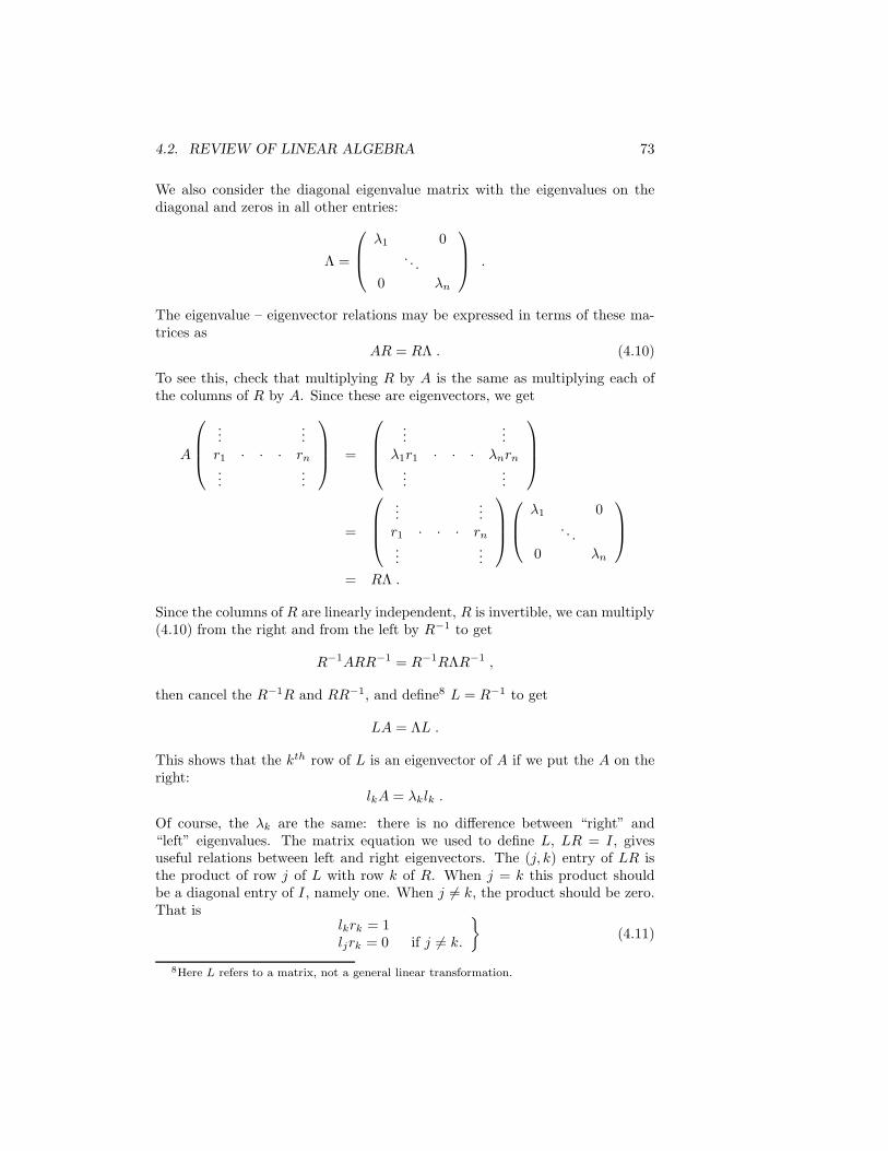
We also consider the diagonal eigenvalue matrix with the eigenvalues on thediagonal and zeros in all other entries:
Λ =
λ1 0. . .
0 λn
.
The eigenvalue – eigenvector relations may be expressed in terms of these ma-trices as
AR = RΛ . (4.10)
To see this, check that multiplying R by A is the same as multiplying each ofthe columns of R by A. Since these are eigenvectors, we get
A
......
r1 · · · rn
......
=
......
λ1r1 · · · λnrn
......
=
......
r1 · · · rn
......
λ1 0. . .
0 λn
= RΛ .
Since the columns of R are linearly independent, R is invertible, we can multiply(4.10) from the right and from the left by R−1 to get
R−1ARR−1 = R−1RΛR−1 ,
then cancel the R−1R and RR−1, and define8 L = R−1 to get
LA = ΛL .
This shows that the kth row of L is an eigenvector of A if we put the A on theright:
lkA = λklk .
Of course, the λk are the same: there is no difference between “right” and“left” eigenvalues. The matrix equation we used to define L, LR = I, givesuseful relations between left and right eigenvectors. The (j, k) entry of LR isthe product of row j of L with row k of R. When j = k this product shouldbe a diagonal entry of I, namely one. When j 6= k, the product should be zero.That is
lkrk = 1ljrk = 0 if j 6= k.
}(4.11)
8Here L refers to a matrix, not a general linear transformation.
74 CHAPTER 4. LINEAR ALGEBRA I, THEORY AND CONDITIONING
These are called biorthogonality relations. For example, r1 need not be orthog-onal to r2, but it is orthogonal to l2. The set of vectors rk is not orthogonal,but the two sets lj and rk are biorthogonal. The left eigenvectors are sometimescalled adjoint eigenvectors because their transposes form right eigenvectors forthe adjoint of A:
A∗l∗j = λj l∗j .
Still supposing n distinct eigenvalues, we may take the right eigenvectors tobe a basis for Rn (or Cn if the entries are not real). As discussed in Section2.2, we may express the action of A in this basis. Since Arj = λjrj , the matrixrepresenting the linear transformation A in this basis will be the diagonal matrixΛ. In the framework of Section 2.2, this is because if we expand a vector v ∈ Rn
in the rk basis, v = v1r1 + · · · + vnrn, then Av = λ1v1r1 + · · · + λnvnrn.For this reason finding a complete set of eigenvectors and eigenvalues is calleddiagonalizing A. A matrix with n linearly independent right eigenvectors isdiagonalizable.
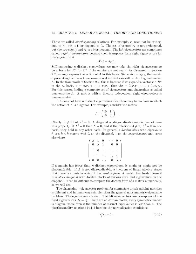
If A does not have n distinct eigenvalues then there may be no basis in whichthe action of A is diagonal. For example, consider the matrix
J =
(0 10 0
).
Clearly, J 6= 0 but J2 = 0. A diagonal or diagonalizable matrix cannot havethis property: if Λ2 = 0 then Λ = 0, and if the relations A 6= 0, A2 = 0 in onebasis, they hold in any other basis. In general a Jordan block with eigenvalueλ is a k × k matrix with λ on the diagonal, 1 on the superdiagonal and zeroselsewhere:
λ 1 0 · · · 00 λ 1 0 0... 0
. . .. . .
......
.... . . λ 1
0 0 · · · 0 λ
.
If a matrix has fewer than n distinct eigenvalues, it might or might not bediagonalizable. If A is not diagonalizable, a theorem of linear algebra statesthat there is a basis in which A has Jordan form. A matrix has Jordan form ifit is block diagonal with Jordan blocks of various sizes and eigenvalues on thediagonal. It can be difficult to compute the Jordan form of a matrix numerically,as we will see.
The eigenvalue – eigenvector problem for symmetric or self-adjoint matricesis different and in many ways simpler than the general nonsymmetric eigenvalueproblem. The eigenvalues are real. The left eigenvectors are transposes of theright eigenvectors: lk = r∗k. There are no Jordan blocks; every symmetric matrixis diagonalizable even if the number of distinct eigenvalues is less than n. Thebiorthogonality relations (4.11) become the normalization conditions
r∗j rj = 1 , (4.12)
4.2. REVIEW OF LINEAR ALGEBRA 75
and the orthogonality relations
r∗j rk = 0 (4.13)
A set of vectors satisfying both (4.12) and (4.13) is called orthonormal. Acomplete set of eigenvectors of a symmetric matrix forms an orthonormal basis.It is easy to check that the orthonormality relations are equivalent to the matrixR in (4.9) satisfying R∗R = I, or, equivalently, R−1 = R∗. Such a matrix iscalled orthogonal. The matrix form of the eigenvalue relation (4.10) may bewritten R∗AR = Λ, or A = RΛR∗, or R∗A = ΛR∗. The latter shows (yetagain) that the rows of R∗, which are r∗k, are left eigenvectors of A.
4.2.6 Differentiation and perturbation theory
The main technique in the perturbation theory of Section 4.3 is implicit dif-ferentiation. We use the formalism of virtual perturbations from mechanicalengineering, which is related to tangent vectors in differential geometry. It mayseem roundabout at first, but it makes actual calculations quick.
Suppose f(x) represents m functions, f1(x), . . . , fm(x) of n variables, x1, . . . , xn.The Jacobian matrix9, f ′(x), is the m×n matrix of partial derivatives f ′
jk(x) =∂xk
fj(x). If f is differentiable (and f ′ is Lipschitz continuous), then the firstderivative approximation is (writing x0 for x to clarify some discussion below)
f(x0 + ∆x) − f(x0) = ∆f = f ′(x0)∆x + O(‖∆x‖2
). (4.14)
Here ∆f and ∆x are column vectors.
Suppose s is a scalar “parameter” and x(s) is a differentiable curve in Rn withx(0) = x0. The function f(x) then defines a curve in Rm with f(x(0)) = f(x0).We define two vectors, called virtual perturbations,
x =dx(s)
ds(0) , f =
df(x(s))
ds(0) .
The multivariate calculus chain rule implies the virtual perturbation formula
f = f ′(x0)x . (4.15)
This formula is nearly the same as (4.14). The virtual perturbation strategy is tocalculate the linear relationship (4.15) between virtual perturbations and use itto find the approximate relation (4.14) between actual perturbations. For this,it is important that any x ∈ Rn can be the virtual perturbation correspondingto some curve: just take the straight “curve” x(s) = x0 + sx.
The Leibnitz rule (product rule) for matrix multiplication makes virtualperturbations handy in linear algebra. Suppose A(s) and B(s) are differentiable
9See any good book on multivariate calculus.
76 CHAPTER 4. LINEAR ALGEBRA I, THEORY AND CONDITIONING
curves of matrices and compatible for matrix multiplication. Then the virtualperturbation of AB is given by the product rule
d
dsAB
∣∣∣∣s=0
= AB + AB . (4.16)
To see this, note that the (jk) entry of A(s)B(s) is∑
l ajl(s)blk(s). Differenti-ating this using the ordinary product rule then setting s = 0 yields
∑
l
ajlblk +∑
l
ajl blk .
These terms correspond to the terms on the right side of (4.16). We can differ-entiate products of more than two matrices in this way.
As an example, consider perturbations of the inverse of a matrix, B = A−1.The variable x in (4.14) now is the matrix A, and f(A) = A−1. Apply implicitdifferentiation to the formula AB = I, use the fact that I is constant, and weget AB + AB = 0. Then solve for B (and use A−1 = B, and get
B = −A−1AA−1 .
The corresponding actual perturbation formula is
∆(A−1
)= −A−1 ∆A A−1 + O
(‖∆A‖2
). (4.17)
This is a generalization of the fact that the derivative of 1/x is −1/x2, so∆(1/x) ≈ −1/x2∆x. When x is replaced by A and ∆A does not commute withA, we have to worry about the order of the factors. The correct order is (4.17).
For future reference we comment on the case m = 1, which is the case ofone function of n variables. The 1 × n Jacobian matrix may be thought of asa row vector. We often write this as ▽f , and calculate it from the fact thatf = ▽f(x) · x for all x. In particular, x is a stationary point of f if ▽f(x) = 0,which is the same as f = 0 for all x. For example, suppose f(x) = x∗Ax forsome n×n matrix A. This is a product of the 1×n matrix x∗ with A with then× 1 matrix x. The Leibnitz rule (4.16) gives, if A is constant,
f = x∗Ax + x∗Ax .
Since the 1× 1 real matrix x∗Ax is equal to its transpose, this is
f = x∗(A + A∗)x .
This implies that (both sides are row vectors)
▽ ( x∗Ax ) = x∗(A + A∗) . (4.18)
If A∗ = A, we recognize this as a generalization of n = 1 formula ddx(ax2) = 2ax.
4.2. REVIEW OF LINEAR ALGEBRA 77
4.2.7 Variational principles for the symmetric eigenvalueproblem
A variational principle is a way to find something by solving a maximization orminimization problem. The Rayleigh quotient for an n× n matrix is
Q(x) =x∗Ax
x∗x=〈x, Ax〉〈x, x〉 . (4.19)
If x is real, x∗ is the transpose of x, which is a row vector. If x is complex, x∗
is the adjoint. In either case, the denominator is x∗x =∑n
k=1 |xk|2 = ‖x‖2l2 .The Rayleigh quotient is defined for x 6= 0. A vector r is a stationary point if▽Q(r) = 0. If r is a stationary point, the corresponding value λ = Q(r) is astationary value.
Theorem 1 If A is a real symmetric or a complex self-adjoint matrix, eacheigenvector of A is a stationary point of the Rayleigh quotient and the cor-responding eigenvalue is the corresponding stationary value. Conversely, eachstationary point of the Rayleigh quotient is an eigenvector and the correspondingstationary value the corresponding eigenvalue.
Proof: We give the proof for real x and real symmetric A. The complex self-adjoint case is an exercise. Underlying the theorem is the calculation (4.18) thatif A∗ = A (this is where symmetry matters) then ▽ ( x∗Ax ) = 2x∗A. Withthis we calculate (using the quotient rule and (4.18) with A = I)
▽Q = 2
(1
x∗x
)x∗A− 2
(x∗Ax
(x∗x)2
)x∗ .
If x is a stationary point (▽Q = 0), then x∗A =(
x∗Axx∗x
)x∗, or, taking the
transpose,
Ax =
(x∗Ax
x∗x
)x .
This shows that x is an eigenvector with
λ =x∗Ax
x∗x= Q(x)
as the corresponding eigenvalue. Conversely if Ar = λr, then Q(r) = λ and thecalculations above show that ▽Q(r) = 0. This proves the theorem.
A simple observation shows that there is at least one stationary point of Qfor Theorem 1 to apply to. If α is a real number, then Q(αx) = Q(x). We maychoose α so that10 ‖αx‖ = 1. This shows that
maxx 6=0
Q(x) = max‖x‖=1
Q(x) = max‖x‖=1
x∗Ax .
10In this section and the next, ‖x‖ = ‖x‖l2 .
78 CHAPTER 4. LINEAR ALGEBRA I, THEORY AND CONDITIONING
A theorem of analysis states that if Q(x) is a continuous function on a compactset, then there is an r so that Q(r) = maxx Q(x) (the max is attained). Theset of x with ‖x‖ = 1 (the unit sphere) is compact and Q is continuous. Clearlyif Q(r) = maxx Q(x), then ▽Q(r) = 0, so r is a stationary point of Q and aneigenvector of A.
The key to finding the other n − 1 eigenvectors is a simple orthogonalityrelation. The principle also is the basis of the singular value decomposition. Ifr is an eigenvector of A and x is orthogonal to r, then x also is orthogonal toAr. Since Ar = λr, and x is orthogonal to r if x∗r = 0, this implies x∗Ar =x∗λr = 0. More generally, suppose we have m < n and eigenvectors r1, . . . , rm.eigenvectors r1, . . . , rm with m < n. Let Vm ⊆ Rn be the set of x ∈ Rn withx∗rj = 0 for j = 1, . . . , m. It is easy to check that this is a subspace of Rn. Theorthogonality principle is that if x ∈ Vm then Ax ∈ Vm. That is, if x∗rj = 0 forall j, then (Ax)∗rj = 0 for all j. But (Ax)∗rj = x∗A∗rj = x∗Arj = x∗λjrj = 0as before.
The variational and orthogonality principles allow us to find n−1 additionalorthonormal eigenvectors as follows. Start with r1, a vector that maximizes Q.Let V1 be the vector space of all x ∈ Rn with r∗1x = 0. We just saw that V1 isan invariant subspace for A, which means that Ax ∈ V1 whenever x ∈ V1. ThusA defines a linear transformation from V1 to V1, which we call A1. Chapter 5.1gives a proof that A1 is symmetric in a suitable basis. Therefore, Theorem 1implies that A1 has at least one real eigenvector, r2, with real eigenvalue λ2.Since r2 ∈ V1, the action of A and A1 on r2 is the same, which means thatAr2 = λ2r2. Also since r2 ∈ V1, r2 is orthogonal to r1. Now let V2 ⊂ V1 be theset of x ∈ V1 with x∗r2 = 0. Since x ∈ V2 means x∗r1 = 0 and x∗r2 = 0, V2 is aninvariant subspace. Thus, there is an r3 ∈ V2 with Ar3 = A1r3 = A2r3 = λ3r3.And again r3 is orthogonal to r2 because r3 ∈ V2 and r3 is orthogonal to r1
because r3 ∈ V2 ⊂ V1. Continuing in this way, we eventually find a full set of northogonal eigenvectors.
4.2.8 Least squares
Suppose A is an m× n matrix representing a linear transformation from Rn toRm, and we have a vector b ∈ Rm. If n < m the linear equation system Ax = bis overdetermined in the sense that there are more equations than variables tosatisfy them. If there is no x with Ax = b, we may seek an x that minimizesthe residual
r = Ax− b . (4.20)
This linear least squares problem
minx‖Ax− b‖l2 , (4.21)
is the same as finding x to minimize the sum of squares
SS =n∑
j=1
r2j .
4.2. REVIEW OF LINEAR ALGEBRA 79
Linear least squares problems arise through linear regression in statistics.A linear regression model models the response, b, as a linear combination ofm explanatory vectors, ak, each weighted by a regression coefficient, xk. Theresidual, R = (
∑mk=1 akxk)−b, is modeled as a Gaussian random variable11 with
mean zero and variance σ2. We do n experiments. The explanatory variables andresponse for experiment j are ajk, for k = 1. . . . , m, and bj , and the residual (forgiven regression coefficients) is rj =
∑mk=1 ajkxk−bj. The log likelihood function
is (r depends on x through (4.20) f(x) = −σ2∑n
j=1 r2j . Finding regression
coefficients to maximize the log likelihood function leads to (4.21).The normal equations give one approach to least squares problems. We
calculate:
‖r‖2l2 = r∗r
= (Ax− b)∗ (Ax− b)
= x∗A∗Ax− 2x∗A∗b + b∗b .
Setting the gradient to zero as in the proof of Theorem 1 leads to the normalequations
A∗Ax = A∗b , (4.22)
which can be solved byx = (A∗A)
−1A∗b . (4.23)
The matrix M = A∗A is the moment matrix or the Gram matrix. It is sym-metric, and positive definite if A has rank m, so the Choleski decomposition ofM (see Chapter 5.1) is a good way to solve (4.22). The matrix (A∗A)−1 A∗
is the pseudoinverse of A. If A were square and invertible, it would be A−1
(check this). The normal equation approach is the fastest way to solve denselinear least squares problems, but it is not suitable for the subtle ill-conditionedproblems that arise often in practice.
The singular value decomposition in Section 4.2.9 and the QR decompositionfrom Section 5.4 give better ways to solve ill-conditioned linear least squaresproblems.
4.2.9 Singular values and principal components
Eigenvalues and eigenvectors of a symmetric matrix have at many applications.They can be used to solve dynamical problems involving A. Because the eigen-vectors are orthogonal, they also determine the l2 norm and condition number ofA. Eigenvalues and eigenvectors of a non-symmetric matrix are not orthogonalso the eigenvalues do not determine the norm or condition number. Singularvalues for non-symmetric or even non-square matrices are a partial substitute.
Let A be an m× n matrix that represents a linear transformation from Rn
to Rm. The right singular vectors, vk ∈ Rn form an orthonormal basis for
11See any good book on statistics for definitions of Gaussian random variable and the loglikelihood function. What is important here is that a systematic statistical procedure, themaximum likelihood method, tells us to minimize the sum of squares of residuals.
80 CHAPTER 4. LINEAR ALGEBRA I, THEORY AND CONDITIONING
Rn. The left singular vectors, uk ∈ Rm, form an orthonormal basis for Rm.Corresponding to each vk and uk pair is a non-negative singular value, σk with
Avk = σkuk . (4.24)
By convention these are ordered so that σ1 ≥ σ2 ≥ · · · ≥ 0. If n < m weinterpret (4.24) as saying that σk = 0 for k > n. If n > m we say σk = 0 fork > m.
The non-zero singular values and corresponding singular vectors may befound one by one using variational and orthogonality principles similar to thosein Section 4.2.7. We suppose A is not the zero matrix (not all entries equal tozero). The first step is the variational principle:
σ1 = maxx 6=0
‖Ax‖‖x‖ . (4.25)
As in Section 4.2.7, the maximum is achieved, and σ1 > 0. Let v1 ∈ Rn be amaximizer, normalized to have ‖v1‖ = 1. Because ‖Av1‖ = σ1, we may writeAv1 = σ1u1 with ‖u1‖ = 1. This is the relation (4.24) with k = 1.
The optimality condition calculated as in the proof of Theorem 1 impliesthat
u∗1A = σ1v
∗1 . (4.26)
Indeed, since σ1 > 0, (4.25) is equivalent to12
σ21 = max
x 6=0
‖Ax‖2
‖x‖2
= maxx 6=0
(Ax)∗(Ax)
x∗x
σ21 = max
x 6=0
x∗(A∗A)x
x∗x. (4.27)
Theorem 1 implies that the solution to the maximization problem (4.27), whichis v1, satisfies σ2v1 = A∗Av1. Since Av1 = σu1, this implies σ1v1 = A∗u1, whichis the same as (4.26).
The analogue of the eigenvalue orthogonality principle is that if x∗v1 = 0,then (Ax)
∗u1 = 0. This is true because
(Ax)∗u1 = x∗ (A∗u1) = x∗σ1v1 = 0 .
Therefore, if we define V1 ⊂ Rn by x ∈ V1 if x∗v1 = 0, and U1 ⊂ Rm by y ∈ U1
if y∗u1 = 0, then A also defines a linear transformation (called A1) from V1 toU1. If A1 is not identically zero, we can define
σ2 = maxx∈V1x 6=0
‖Ax‖2
‖x‖2= max
x∗v1=0x 6=0
‖Ax‖2
‖x‖2,
12These calculations make constant use of the associativity of matrix multiplication, evenwhen one of the matrices is a row or column vector.
4.3. CONDITION NUMBER 81
and get Av2 = σ2u2 with v∗2v1 = 0 and u∗2u1 = 0. This is the second step
constructing orthonormal bases satisfying (4.24). Continuing in this way, wecan continue finding orthonormal vectors vk and uk that satisfy (4.24) untilreach Ak = 0 or k = m or k = n. After that point, the may complete the v andu bases arbitrarily as in Chapter 5.1 with remaining singular values being zero.
The singular value decomposition (SVD) is a matrix expression of the rela-tions (4.24). Let U be the m ×m matrix whose columns are the left singularvectors uk (as in (4.9)). The orthonormality relations u∗
juk = δjk are equivalentto U being an orthogonal matrix: U∗U = I. Similarly, we can form the orthog-onal n× n matrix, V , whose columns are the right singular vectors vk. Finally,the m × n matrix, Σ, has the singular values on its diagonal (with somewhatunfortunate notation), σjj = σj , and zeros off the diagonal, σjk = 0 if j 6= k.With these definitions, the relations (4.24) are equivalent to AV = UΣ, whichmore often is written
A = UΣV ∗ . (4.28)
This the singular value decomposition. Any matrix may be factored, or decom-posed, into the product of the form (4.28) where U is an m × m orthogonalmatrix, Σ is an m × n diagonal matrix with nonnegative entries, and V is ann× n orthogonal matrix.
A calculation shows that A∗A = V Σ∗ΣV ∗ = V ΛV ∗. This implies that theeigenvalues of A∗A are given by λj = σ2
j and the right singular vectors of A
are the eigenvectors of A∗A. It also implies that κl2(A∗A) = κl2(A)2. This
means that the condition number of solving the normal equations (4.22) is thesquare of the condition number of the original least squares problem (4.21).If the condition number of a least squares problem is κl2(A) = 105, even thebest solution algorithm can amplify errors by a factor of 105. Solving using thenormal equations can amplify rounding errors by a factor of 1010.
Many people call singular vectors uk and vk principal components. Theyrefer to the singular value decomposition as principal component analysis, orPCA. One application is clustering, in which you have n objects, each with mmeasurements, and you want to separate them into two clusters, say “girls”and “boys”. You assemble the data into a matrix, A, and compute, say, thelargest two singular values and corresponding left singular vectors, u1 ∈ Rm
and u2 ∈ Rm. The data for object k is ak ∈ Rm, and you compute zk ∈ R2 byzk1 = u∗
1ak and zk2 = u∗2ak, the components of ak in the principal component
directions. You then plot the n points zk in the plane and look for clusters, ormaybe just a line that separates one group of points from another. Surprisingas may seem, this simple procedure does identify clusters in practical problems.
4.3 Condition number
Ill-conditioning can be a serious problem in numerical solution of problems inlinear algebra. We take into account possible ill-conditioning when we choosecomputational strategies. For example, the matrix exponential exp(A) (seeexercise 12) can be computed using the eigenvectors and eigenvalues of A. We
82 CHAPTER 4. LINEAR ALGEBRA I, THEORY AND CONDITIONING
will see in Section 4.3.3 that the eigenvalue problem may be ill conditioned evenwhen the problem of computing exp(A) is fine. In such cases we need a way tocompute exp(A) that does not use the eigenvectors and eigenvalues of A.
As we said in Section 2.7 (in slightly different notation), the condition num-ber is the ratio of the change in the answer to the change in the problem data,with (i) both changed measured in relative terms, and (ii) the change in theproblem data being small. Norms allow us to make this definition more precisein the case of multivariate functions and data. Let f(x) represent m functionsof n variables, with ∆x being a change in x and ∆f = f(x + ∆x) − f(x) thecorresponding change in f . The size of ∆x, relative to x is ‖∆x‖ / ‖x‖, andsimilarly for ∆f . In the multivariate case, the size of ∆f depends not only onthe size of ∆x, but also on the direction. The norm based condition numberseeks the worst case ∆x, which leads to
κ(x) = limǫ→0
max‖∆x‖=ǫ
‖f(x+∆x)−f(x)‖‖f(x)‖‖∆x‖‖x‖
. (4.29)
Except for the maximization over directions ∆x with ‖∆x‖ = ǫ, this is the sameas the earlier definition 2.8.
Still following Section 2.7, we express (4.29) in terms of derivatives of f . Welet f ′(x) represent the m×n Jacobian matrix of first partial derivatives of f , as in
Section 4.2.6, so that, ∆f = f ′(x)∆x+O(‖∆x‖2
). Since O
(‖∆x‖2
)/ ‖∆x‖ =
O (‖∆x‖), the ratio in (4.29) may be written
‖∆f‖‖∆x‖ ·
‖x‖‖f‖ =
‖f ′(x)∆x‖‖∆x‖ · ‖x‖‖f‖ + O (‖∆x‖) .
The second term on the right disappears as ∆x→ 0. Maximizing the first termon the right over ∆x yields the norm of the matrix f ′(x). Altogether, we have
κ(x) = ‖f ′(x)‖ · ‖x‖‖f(x)‖ . (4.30)
This differs from the earlier condition number definition (2.10) in that it usesnorms and maximizes over ∆x with ‖∆x‖ = ǫ.
In specific calculations we often use a slightly more complicated way of stat-ing the definition (4.29). Suppose that P and Q are two positive quantities andthere is a C so that P ≤ C · Q. We say that C is the sharp constant if thereis no C′ with C′ < C so that P ≤ C′ ·Q. For example, we have the inequalitysin(2ǫ) ≤ 3 · ǫ for all x. But C = 3 is not the sharp constant because the in-equality also is true with C′ = 2, which is sharp. But this definition is clumsy,for example, if we ask for the sharp constant in the inequality tan(ǫ) ≤ C · ǫ.For one thing, we must restrict to ǫ→ 0. The sharp constant should be C = 1because if C′ > 1, there is an ǫ0 so that if ǫ ≤ ǫ0, then tan(ǫ) ≤ C′ · ǫ. But theinequality is not true with C = 1 for any ǫ. Therefore we write
P (ǫ)≤∼CQ(ǫ) as ǫ→ 0 (4.31)
4.3. CONDITION NUMBER 83
if
limǫ→0
P (ǫ)
Q(ǫ)≤ C .
In particular, we can seek the sharp constant, the smallest C so that
P (ǫ) ≤ C ·Q(ǫ) + O(ǫ) as ǫ→ 0.
The definition (??) is precisely that κ(x) is the sharp constant in the inequality
‖∆f‖‖f‖
≤∼‖∆x‖‖x‖ as ‖x‖ → 0. (4.32)
4.3.1 Linear systems, direct estimates
We start with the condition number of calculating b = Au in terms of u with Afixed. This fits into the general framework above, with u playing the role of x,and Au of f(x). Of course, A is the Jacobian of the function u→ Au, so (4.30)gives
κ(A, u) = ‖A‖ · ‖u‖‖Au‖ . (4.33)
The condition number of solving a linear system Au = b (finding u as a functionof b) is the same as the condition number of the computation u = A−1b. Theformula (4.33) gives this as
κ(A−1, b) =∥∥A−1
∥∥ · ‖b‖‖A−1b‖ = ‖A−1‖ · ‖Au‖
‖u‖ .
For future reference, not that this is not the same as (4.33).The traditional definition of the condition number of the Au computation
takes the worst case relative error not only over perturbations ∆u but also overvectors u. Taking the maximum over ∆u led to (4.33), so we need only maximizeit over u:
κ(A) = ‖A‖ ·maxu6=0
‖u‖‖Au‖ . (4.34)
Since A(u + ∆u)−Au = A∆u, and u and ∆u are independent variables, this isthe same as
κ(A) = maxu6=0
‖u‖‖Au‖ · max
∆u6=0
‖A∆u‖‖∆u‖ . (4.35)
To evaluate the maximum, we suppose A−1 exists.13 Substituting Au = v,u = A−1v, gives
maxu6=0
‖u‖‖Au‖ = max
v 6=0
∥∥A−1v∥∥
‖v‖ =∥∥A−1
∥∥ .
13See exercise 8 for a the l2 condition number of the u → Au problem with singular ornon-square A.
84 CHAPTER 4. LINEAR ALGEBRA I, THEORY AND CONDITIONING
Thus, (4.34) leads to
κ(A) = ‖A‖∥∥A−1
∥∥ (4.36)
as the worst case condition number of the forward problem.
The computation b = Au with
A =
(1000 0
0 10
)
illustrates this discussion. The error amplification relates ‖∆b‖ / ‖b‖ to ‖∆u‖ / ‖u‖.The worst case would make ‖b‖ small relative to ‖u‖ and ‖∆b‖ large relativeto ‖∆u‖: amplify u the least and ∆u the most. This is achieved by taking
u =
(01
)so that Au =
(0
10
)with amplification factor 10, and ∆u =
(ǫ0
)
with A∆u =
(1000ǫ
0
)and amplification factor 1000. This makes ‖∆b‖ / ‖b‖
100 times larger than ‖∆u‖ / ‖u‖. For the condition number of calculating
u = A−1b, the worst case is b =
(01
)and ∆b =
(ǫ0
), which amplifies the error
by the same factor of κ(A) = 100.
The informal condition number (4.34) has advantages and disadvantages overthe more formal one (4.33). At the time we design a computational strategy,it may be easier to estimate the informal condition number than the formalone, as we may know more about A than u. If we have no idea what u willcome up, we have a reasonable chance of getting something like the worst one.Moreover, κ(A) defined by (4.34) determines the convergence rate of iterativestrategies for solving linear systems involving A. On the other hand, there arecases, particularly when solving partial differential equations, where κ(A) ismuch more pessimistic than κ(A, u). For example, in Exercise 11, κ(A) is onthe order of n2, where n is the number of unknowns. The truncation error forthe second order discretization is on the order of 1/n2. A naive estimate using(4.34) might suggest that solving the system amplifies the O(n−2) truncationerror by a factor of n2 to be on the same order as the solution itself. This doesnot happen because the u we seek is smooth, and not like the worst case.
The informal condition number (4.36) also has the strange feature than
κ(A) = κ(A−1), since(A−1
)−1= A. For one thing, this is not true, even using
informal definitions, for nonlinear problems. Moreover, it is untrue in importantlinear problems, such as the heat equation.14 Computing the solution at timet > 0 from “initial data” at time zero is a linear process that is well conditionedand numerically stable. Computing the solution at time zero from the solutionat time t > 0 is so ill conditioned as to be essentially impossible. Again, themore precise definition (4.33) does not have this drawback.
14See, for example, the book by Fritz John on partial differential equations.
4.3. CONDITION NUMBER 85
4.3.2 Linear systems, perturbation theory
If Au = b, we can study the dependence of u on A through perturbation theory.The starting point is the perturbation formula (4.17). Taking norms gives
‖∆u‖ <≈∥∥A−1
∥∥ ‖∆A‖ ‖u‖ , (for small ∆A), (4.37)
so‖∆u‖‖u‖
<≈∥∥A−1
∥∥ ‖A‖ · ‖∆A‖‖A‖ (4.38)
This shows that the condition number satisfies κ ≤∥∥A−1
∥∥ ‖A‖. The condition
number is equal to∥∥A−1
∥∥ ‖A‖ if the inequality (4.37) is (approximately for small∆A) sharp, which it is because we can take ∆A = ǫI and u to be a maximumstretch vector for A−1.
We summarize with a few remarks. First, the condition number formula(4.36) applies to the problem of solving the linear system Au = b both when weconsider perturbations in b and in A, though the derivations here are different.However, this is not the condition number in the strict sense of (4.29) and(4.30) because the formula (4.36) assumes taking the worst case over a family ofproblems (varying b in this case), not just over all possible small perturbations inthe data. Second, the formula (4.36) is independent of the size of A. ReplacingA with cA leaves κ(A) unchanged. What matters is the ratio of the maximumto minimum stretch, as in (4.35).
4.3.3 Eigenvalues and eigenvectors
The eigenvalue relationship is Arj = λjrj . Perturbation theory allows to esti-mate the changes in λj and rj that result from a small ∆A. These perturbationresults are used throughout science and engineering. We begin with the sym-metric or self-adjoint case, it often is called Rayleigh Schodinger perturbationtheory15 Using the virtual perturbation method of Section 4.2.6, differentiatingthe eigenvalue relation using the product rule yields
Arj + Arj = λjrj + λj rj . (4.39)
Multiply this from the left by r∗j and use the fact that r∗j is a left eigenvector16
givesr∗j Ajrj = λlr
∗j rj .
If rj is normalized so that r∗j rj = ‖rj‖2l2 = 1, then the right side is just λj .Trading virtual perturbations for actual small perturbations turns this into thefamous formula
∆λj = r∗j ∆A rj + O(‖∆A‖2
). (4.40)
15Lord Rayleigh used it to study vibrational frequencies of plates and shells. Later ErwinSchrodinger used it to compute energies (which are eigenvalues) in quantum mechanics.
16Arj = λjrj ⇒ (Arj)∗ = (λjrj)
∗ ⇒ r∗jA = λjr∗
jsince A∗ = A and λj is real.
86 CHAPTER 4. LINEAR ALGEBRA I, THEORY AND CONDITIONING
We get a condition number estimate by recasting this in terms of rela-tive errors on both sides. The important observation is that ‖rj‖l2 = 1, so‖∆A · rj‖l2 ≤ ‖∆A‖l2 and finally
∣∣r∗j ∆A rj
∣∣ ≤≈ ‖∆A‖l2 .
This inequality is sharp because we can take ∆A = ǫrjr∗j , which is an n × n
matrix with (see exercise 7)∥∥ǫrjr
∗j
∥∥l2
= |ǫ|. Putting this into (4.40) gives thealso sharp inequality, ∣∣∣∣
∆λj
λj
∣∣∣∣ ≤‖A‖l2|λj |
‖∆A‖l2‖A‖l2
.
We can put this directly into the abstract condition number definition (4.29) toget the conditioning of λj :
κj(A) =‖A‖l2|λj |
=|λ|max
|λj |(4.41)
Here, κj(A) denotes the condition number of the problem of computing λj ,which is a function of the matrix A, and ‖A‖l2 = |λ|max refers to the eigenvalueof largest absolute value.
The condition number formula (4.41) predicts the sizes of errors we get inpractice. Presumably λj depends in some way on all the entries of A and theperturbations due to roundoff will be on the order of the entries themselves,multiplied by the machine precision, ǫmach, which are on the order of ‖A‖. Onlyif λj is very close to zero, by comparison with |λmax|, will it be hard to computewith high relative accuracy. All of the other eigenvalue and eigenvector problemshave much worse condition number difficulties.
The eigenvalue problem for non-symmetric matrices can by much more sen-sitive. To derive the analogue of (4.40) for non-symmetric matrices we startwith (4.39) and multiply from the left with the corresponding left eigenvector,lj . After simplifying, the result is
λj = ljArj , ∆λj = lj∆Arj + O(‖∆A‖2
). (4.42)
In the non-symmetric case, the eigenvectors need not be orthogonal and theeigenvector matrix R need not be well conditioned. For this reason, it is possiblethat lk, which is a row of R−1 is very large. Working from (4.42) as we did forthe symmetric case leads to
∣∣∣∣∆λj
λj
∣∣∣∣ ≤ κLS(R)‖A‖|λj |‖∆A‖‖A‖ .
Here κLS(R) =∥∥R−1
∥∥ ‖R‖ is the linear systems condition number of the righteigenvector matrix. Therefore, the condition number of the non-symmetriceigenvalue problem is (again because the inequalities are sharp)
κj(A) = κLS(R)‖A‖|λj |
. (4.43)
4.4. SOFTWARE 87
Since A is not symmetric, we cannot replace ‖A‖ by |λ|max as we did for (4.41).In the symmetric case, the only reason for ill-conditioning is that we are lookingfor a (relatively) tiny number. For non-symmetric matrices, it is also possiblethat the eigenvector matrix is ill-conditioned. It is possible to show that ifa family of matrices approaches a matrix with a Jordan block, the conditionnumber of R approaches infinity. For a symmetric or self-adjoint matrix, R isorthogonal or unitary, so that ‖R‖l2 = ‖R∗‖l2 = 1 and κLS(R) = 1.
The eigenvector perturbation theory uses the same ideas, with the extratrick of expanding the derivatives of the eigenvectors in terms of the eigenvectorsthemselves. We expand the virtual perturbation rj in terms of the eigenvectorsrk. Call the expansion coefficients mjk, and we have
rj =
n∑
l=1
mjlrl .
For the symmetric eigenvalue problem, if all the eigenvalues are distinct, theformula follows from multiplying (4.39) from the left by r∗k:
mjk =r∗kArj
λj − λk,
so that
∆rj =∑
k 6=j
r∗k∆Arj
λj − λk+ O
(‖∆A‖2
).
(The term j = k is omitted because mjj = 0: differentiating r∗j rj = 1 givesr∗j rj = 0.) This shows that the eigenvectors have condition number “issues”even when the eigenvalues are well-conditioned, if the eigenvalues are close toeach other. Since the eigenvectors are not uniquely determined when eigenvaluesare equal, this seems plausible. The unsymmetric matrix perturbation formulais
mkj =ljArk
λj − λk.
Again, we have the potential problem of an ill-conditioned eigenvector basis,combined with the possibility of close eigenvalues. The conclusion is that theeigenvector conditioning can be problematic, even though the eigenvalues arefine, for closely spaced eigenvalues.
4.4 Software
4.4.1 Software for numerical linear algebra
There have been major government-funded efforts to produce high quality soft-ware for numerical linear algebra. This culminated in the public domain softwarepackage LAPack. LAPack is a combination and extension of earlier packagesEispack, for solving eigenvalue problems, and Linpack, for solving systems of
88 CHAPTER 4. LINEAR ALGEBRA I, THEORY AND CONDITIONING
equations. Many of the high quality components of Eispack and Linpack alsowere incorporated into Matlab, which accounts for the high quality of Matlablinear algebra routines.
Our software advice is to use LAPack or Matlab software for computationallinear algebra whenever possible. It is worth the effort in coax the LAPack make
files to work in a particular computing environment. You may avoid wastingtime coding algorithms that have been coded thousands of times before, oryou may avoid suffering from the subtle bugs of the codes you got from nextdoor that came from who knows where. The professional software often does itbetter, for example using balancing algorithms to improve condition numbers.The professional software also has clever condition number estimates that oftenare more sophisticated than the basic algorithms themselves.
4.4.2 Test condition numbers
Part of the error flag in linear algebra computation is the condition number.Accurate computation of the condition number may be more expensive thanthe problem at hand. For example, computing ‖A‖
∥∥A−1∥∥ is more several times
more expensive than solving Ax = b. However, there are cheap heuristics thatgenerally are reliable, at least for identifying severe ill-conditioning. If the con-dition number is so large that all relative accuracy in the data is lost, the routineshould return an error flag. Using such condition number estimates makes thecode slightly slower, but it makes the computed results much more trustworthy.
4.5 Resources and further reading
If you need to review linear algebra, the Schaum’s Outline review book on Lin-ear Algebra may be useful. For a practical introduction to linear algebra writtenby a numerical analyst, try the book by Gilbert Strang. More theoretical treat-ments may be found in the book by Peter Lax or the one by Paul Halmos.An excellent discussion of condition number is given in the SIAM lecture notesof Lloyd N. Trefethen. Beresford Parlett has a nice but somewhat out-of-datebook on the theory and computational methods for the symmetric eigenvalueproblem. The Linear Algebra book by Peter Lax also has a beautiful discussionof eigenvalue perturbation theory and some of its applications. More applica-tions may be found in the book Theory of Sound by Lord Rayleigh (reprintedby Dover Press) and in any book on quantum mechanics. I do not know an ele-mentary book that covers perturbation theory for the non-symmetric eigenvalueproblem in a simple way.
The software repository Netlib, http://netlib.org, is a source for LAPack.Other sources of linear algebra software, including Mathematica and Numeri-cal Recipes, are not recommended. Netlib also has some of the best availablesoftware for solving sparse linear algebra problems.
4.6. EXERCISES 89
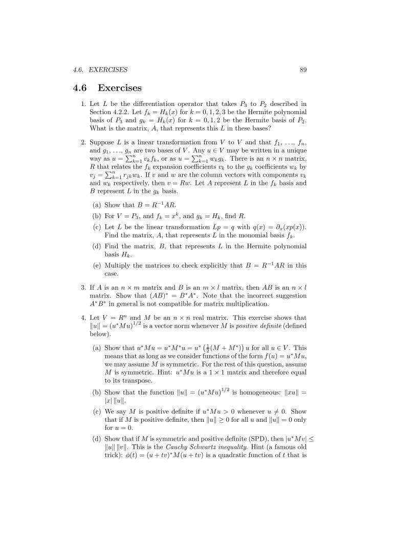
4.6 Exercises
1. Let L be the differentiation operator that takes P3 to P2 described inSection 4.2.2. Let fk = Hk(x) for k = 0, 1, 2, 3 be the Hermite polynomialbasis of P3 and gk = Hk(x) for k = 0, 1, 2 be the Hermite basis of P2.What is the matrix, A, that represents this L in these bases?
2. Suppose L is a linear transformation from V to V and that f1, . . ., fn,and g1, . . ., gn are two bases of V . Any u ∈ V may be written in a uniqueway as u =
∑nk=1 vkfk, or as u =
∑nk=1 wkgk. There is an n× n matrix,
R that relates the fk expansion coefficients vk to the gk coefficients wk byvj =
∑nk=1 rjkwk. If v and w are the column vectors with components vk
and wk respectively, then v = Rw. Let A represent L in the fk basis andB represent L in the gk basis.
(a) Show that B = R−1AR.
(b) For V = P3, and fk = xk, and gk = Hk, find R.
(c) Let L be the linear transformation Lp = q with q(x) = ∂x(xp(x)).Find the matrix, A, that represents L in the monomial basis fk.
(d) Find the matrix, B, that represents L in the Hermite polynomialbasis Hk.
(e) Multiply the matrices to check explicitly that B = R−1AR in thiscase.
3. If A is an n ×m matrix and B is an m × l matrix, then AB is an n × lmatrix. Show that (AB)∗ = B∗A∗. Note that the incorrect suggestionA∗B∗ in general is not compatible for matrix multiplication.
4. Let V = Rn and M be an n × n real matrix. This exercise shows that‖u‖ = (u∗Mu)
1/2is a vector norm whenever M is positive definite (defined
below).
(a) Show that u∗Mu = u∗M∗u = u∗ ( 12 (M + M∗)
)u for all u ∈ V . This
means that as long as we consider functions of the form f(u) = u∗Mu,we may assume M is symmetric. For the rest of this question, assumeM is symmetric. Hint: u∗Mu is a 1 × 1 matrix and therefore equalto its transpose.
(b) Show that the function ‖u‖ = (u∗Mu)1/2
is homogeneous: ‖xu‖ =|x| ‖u‖.
(c) We say M is positive definite if u∗Mu > 0 whenever u 6= 0. Showthat if M is positive definite, then ‖u‖ ≥ 0 for all u and ‖u‖ = 0 onlyfor u = 0.
(d) Show that if M is symmetric and positive definite (SPD), then |u∗Mv| ≤‖u‖ ‖v‖. This is the Cauchy Schwartz inequality. Hint (a famous oldtrick): φ(t) = (u + tv)∗M(u + tv) is a quadratic function of t that is
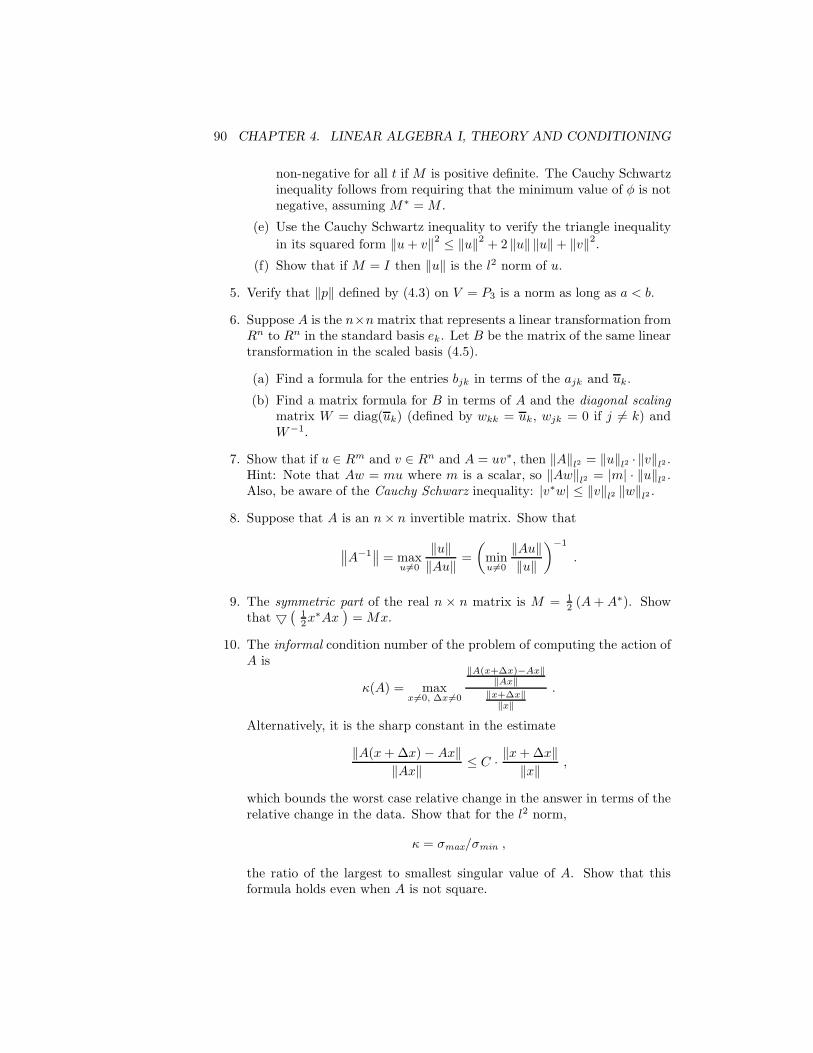
90 CHAPTER 4. LINEAR ALGEBRA I, THEORY AND CONDITIONING
non-negative for all t if M is positive definite. The Cauchy Schwartzinequality follows from requiring that the minimum value of φ is notnegative, assuming M∗ = M .
(e) Use the Cauchy Schwartz inequality to verify the triangle inequality
in its squared form ‖u + v‖2 ≤ ‖u‖2 + 2 ‖u‖ ‖u‖+ ‖v‖2.(f) Show that if M = I then ‖u‖ is the l2 norm of u.
5. Verify that ‖p‖ defined by (4.3) on V = P3 is a norm as long as a < b.
6. Suppose A is the n×n matrix that represents a linear transformation fromRn to Rn in the standard basis ek. Let B be the matrix of the same lineartransformation in the scaled basis (4.5).
(a) Find a formula for the entries bjk in terms of the ajk and uk.
(b) Find a matrix formula for B in terms of A and the diagonal scalingmatrix W = diag(uk) (defined by wkk = uk, wjk = 0 if j 6= k) andW−1.
7. Show that if u ∈ Rm and v ∈ Rn and A = uv∗, then ‖A‖l2 = ‖u‖l2 · ‖v‖l2 .Hint: Note that Aw = mu where m is a scalar, so ‖Aw‖l2 = |m| · ‖u‖l2 .Also, be aware of the Cauchy Schwarz inequality: |v∗w| ≤ ‖v‖l2 ‖w‖l2 .
8. Suppose that A is an n× n invertible matrix. Show that
∥∥A−1∥∥ = max
u6=0
‖u‖‖Au‖ =
(minu6=0
‖Au‖‖u‖
)−1
.
9. The symmetric part of the real n × n matrix is M = 12 (A + A∗). Show
that ▽(
12x∗Ax
)= Mx.
10. The informal condition number of the problem of computing the action ofA is
κ(A) = maxx 6=0, ∆x 6=0
‖A(x+∆x)−Ax‖‖Ax‖
‖x+∆x‖‖x‖
.
Alternatively, it is the sharp constant in the estimate
‖A(x + ∆x) −Ax‖‖Ax‖ ≤ C · ‖x + ∆x‖
‖x‖ ,
which bounds the worst case relative change in the answer in terms of therelative change in the data. Show that for the l2 norm,
κ = σmax/σmin ,
the ratio of the largest to smallest singular value of A. Show that thisformula holds even when A is not square.
4.6. EXERCISES 91
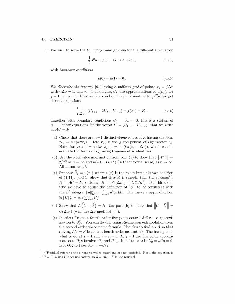
11. We wish to solve the boundary value problem for the differential equation
1
2∂2
xu = f(x) for 0 < x < 1, (4.44)
with boundary conditions
u(0) = u(1) = 0 . (4.45)
We discretize the interval [0, 1] using a uniform grid of points xj = j∆xwith n∆x = 1. The n− 1 unknowns, Uj , are approximations to u(xj), forj = 1, . . . , n− 1. If we use a second order approximation to 1
2∂2xu, we get
discrete equations
1
2
1
∆x2(Uj+1 − 2Uj + Uj−1) = f(xj) = Fj . (4.46)
Together with boundary conditions U0 = Un = 0, this is a system ofn − 1 linear equations for the vector U = (U1, . . . , Un−1)
∗ that we writeas AU = F .
(a) Check that there are n−1 distinct eigenvectors of A having the formrkj = sin(kπxj). Here rkj is the j component of eigenvector rk.Note that rk,j+1 = sin(kπxj+1) = sin(kπ(xj + ∆x)), which can beevaluated in terms of rkj using trigonometric identities.
(b) Use the eigenvalue information from part (a) to show that∥∥A−1
∥∥→2/π2 as n→∞ and κ(A) = O(n2) (in the informal sense) as n→∞.All norms are l2.
(c) Suppose Uj = u(xj) where u(x) is the exact but unknown solutionof (4.44), (4.45). Show that if u(x) is smooth then the residual17,
R = AU − F , satisfies ‖R‖ = O(∆x2) = O(1/n2). For this to betrue we have to adjust the definition of ‖U‖ to be consistent with
the L2 integral ‖u‖2L2 =∫ 1
x=0u2(x)dx. The discrete approximation
is ‖U‖2l2 = ∆x∑n
k=1 U2j .
(d) Show that A(U − U
)= R. Use part (b) to show that
∥∥∥U − U∥∥∥ =
O(∆x2) (with the ∆x modified ‖·‖).(e) (harder) Create a fourth order five point central difference approxi-
mation to ∂2xu. You can do this using Richardson extrapolation from
the second order three point formula. Use this to find an A so thatsolving AU = F leads to a fourth order accurate U . The hard part iswhat to do at j = 1 and j = n− 1. At j = 1 the five point approxi-mation to ∂2
xu involves U0 and U−1. It is fine to take U0 = u(0) = 0.Is it OK to take U−1 = −U1?
17Residual refers to the extent to which equations are not satisfied. Here, the equation is
AU = F , which U does not satisfy, so R = AU − F is the residual.
92 CHAPTER 4. LINEAR ALGEBRA I, THEORY AND CONDITIONING
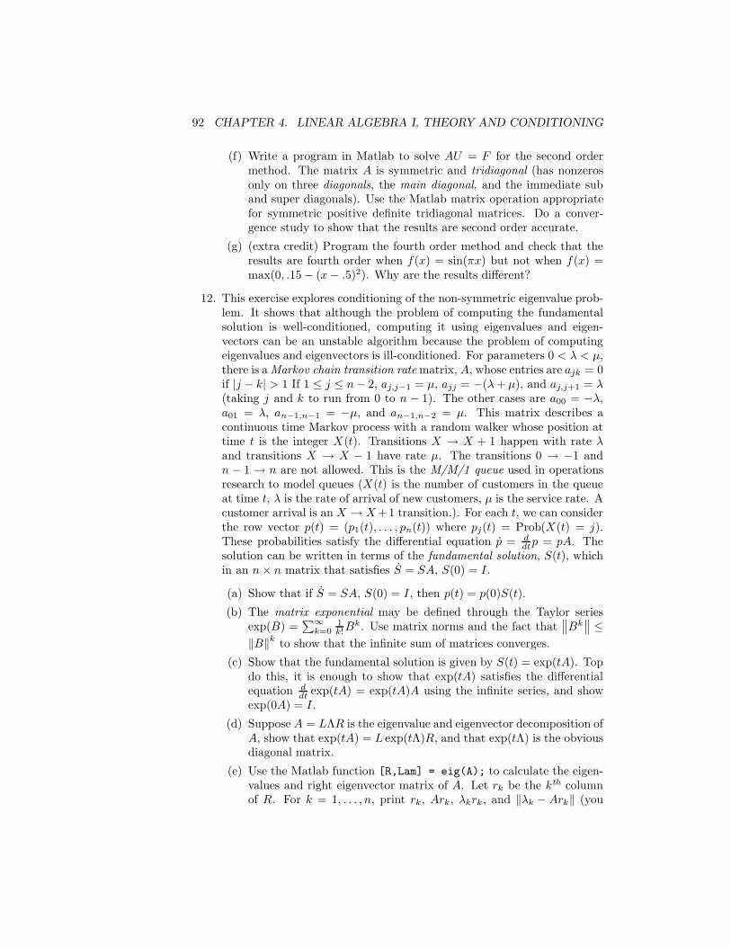
(f) Write a program in Matlab to solve AU = F for the second ordermethod. The matrix A is symmetric and tridiagonal (has nonzerosonly on three diagonals, the main diagonal, and the immediate suband super diagonals). Use the Matlab matrix operation appropriatefor symmetric positive definite tridiagonal matrices. Do a conver-gence study to show that the results are second order accurate.
(g) (extra credit) Program the fourth order method and check that theresults are fourth order when f(x) = sin(πx) but not when f(x) =max(0, .15− (x− .5)2). Why are the results different?
12. This exercise explores conditioning of the non-symmetric eigenvalue prob-lem. It shows that although the problem of computing the fundamentalsolution is well-conditioned, computing it using eigenvalues and eigen-vectors can be an unstable algorithm because the problem of computingeigenvalues and eigenvectors is ill-conditioned. For parameters 0 < λ < µ,there is a Markov chain transition rate matrix, A, whose entries are ajk = 0if |j − k| > 1 If 1 ≤ j ≤ n− 2, aj,j−1 = µ, ajj = −(λ + µ), and aj,j+1 = λ(taking j and k to run from 0 to n − 1). The other cases are a00 = −λ,a01 = λ, an−1,n−1 = −µ, and an−1,n−2 = µ. This matrix describes acontinuous time Markov process with a random walker whose position attime t is the integer X(t). Transitions X → X + 1 happen with rate λand transitions X → X − 1 have rate µ. The transitions 0 → −1 andn − 1 → n are not allowed. This is the M/M/1 queue used in operationsresearch to model queues (X(t) is the number of customers in the queueat time t, λ is the rate of arrival of new customers, µ is the service rate. Acustomer arrival is an X → X +1 transition.). For each t, we can considerthe row vector p(t) = (p1(t), . . . , pn(t)) where pj(t) = Prob(X(t) = j).These probabilities satisfy the differential equation p = d
dtp = pA. Thesolution can be written in terms of the fundamental solution, S(t), whichin an n× n matrix that satisfies S = SA, S(0) = I.
(a) Show that if S = SA, S(0) = I, then p(t) = p(0)S(t).
(b) The matrix exponential may be defined through the Taylor seriesexp(B) =
∑∞k=0
1k!B
k. Use matrix norms and the fact that∥∥Bk
∥∥ ≤‖B‖k to show that the infinite sum of matrices converges.
(c) Show that the fundamental solution is given by S(t) = exp(tA). Topdo this, it is enough to show that exp(tA) satisfies the differentialequation d
dt exp(tA) = exp(tA)A using the infinite series, and showexp(0A) = I.
(d) Suppose A = LΛR is the eigenvalue and eigenvector decomposition ofA, show that exp(tA) = L exp(tΛ)R, and that exp(tΛ) is the obviousdiagonal matrix.
(e) Use the Matlab function [R,Lam] = eig(A); to calculate the eigen-values and right eigenvector matrix of A. Let rk be the kth columnof R. For k = 1, . . . , n, print rk, Ark, λkrk, and ‖λk −Ark‖ (you
4.6. EXERCISES 93
choose the norm). Mathematically, one of the eigenvectors is a mul-tiple of the vector 1 defined in part h. The corresponding eigenvalueis λ = 0. The computed eigenvalue is not exactly zero. Take n = 4for this, but do not hard wire n = 4 into the Matlab code.
(f) Let L = R−1, which can be computed in Matlab using L=R^(-1);.Let lk be the kth row of L, check that the lk are left eigenvectors ofA as in part e. Corresponding to λ = 0 is a left eigenvector that is amultiple of p∞ from part h. Check this.
(g) Write a program in Matlab to calculate S(t) using the eigenvalues andeigenvectors of A as above. Compare the results to those obtainedusing the Matlab built in function S = expm(t*A);. Use the valuesλ = 1, µ = 4, t = 1, and n ranging from n = 4 to n = 80. Comparethe two computed S(t) (one using eigenvalues, the other just usingexpm) using the l1 matrix norm. Use the Matlab routine cond(R) tocompute the condition number of the eigenvector matrix, R. Printthree columns of numbers, n, error, condition number. Comment onthe quantitative relation between the error and the condition number.
(h) Here we figure out which of the answers is correct. To do this, use theknown fact that limt→∞ S(t) = S∞ has the simple form S∞ = 1p∞,where 1 is the column vector with all ones, and p∞ is the row vectorwith p∞,j = ((1 − r)/(1 − rn))rj , with r = λ/µ. Take t = 3 ∗ n(which is close enough to t = ∞ for this purpose) and the samevalues of n and see which version of S(t) is correct. What can yousay about the stability of computing the matrix exponential usingthe ill conditioned eigenvalue/eigenvector problem?
13. This exercise explores eigenvalue and eigenvector perturbation theory forthe matrix A defined in exercise 12. Let B be the n × n matrix withbjk = 0 for all (j, k) except b00 = −1 and b1,n−1 = 1 (as in exercise 12,indices run from j = 0 to j = n − 1). Define A(s) = A + sB, so that
A(0) = A and dA(s)ds = B when s = 0.
(a) For n = 20, print the eigenvalues of A(s) for s = 0 and s = .1.What does this say about the condition number of the eigenvalueeigenvector problem? All the eigenvalues of a real tridiagonal matrixare real18 but that A(s = .1) is not tridiagonal and its eigenvaluesare not real.
(b) Use first order eigenvalue perturbation theory to calculate λk = ddsλk
when s = 0. What size s do you need for ∆λk to be accuratelyapproximated by sλk? Try n = 5 and n = 20. Note that first orderperturbation theory always predicts that eigenvalues stay real, sos = .1 is much too large for n = 20.
18It is easy to see that if A is tridiagonal then there is a diagonal matrix, W , so that WAW−1
is symmetric. Therefore, A has the same eigenvalues as the symmetric matrix WAW−1.

94 CHAPTER 4. LINEAR ALGEBRA I, THEORY AND CONDITIONING