Embed Size (px)
Citation preview
1st
Semester
Linear Algebra I
Prepared by
Modern University
for Technology &Information
Faculty of Computers & Artificial
Intelligence
Prof. Dr. Eiman Abou El-Dahab
Level One
Modern University for Technology
&Information
Faculty of Computers & Artificial Intelligence
Department of Basic Science
Linear Algebra I
Prof. Dr. Eiman Taha Abou El Dahab
Table of content
I
Table of Contents
C H A P T E R ONE ........................................................................................................ - 1 -
1.2 Gaussian Elimination ........................................................................................... - 16 -
Exercise Set 1.2 .......................................................................................................... - 21 -
1.3 Matrices and Matrix Operations ......................................................................... - 26 -
Exercise set 1.3 .......................................................................................................... - 35 -
1.4 Inverses; Algebraic Properties of Matrices ......................................................... - 39 -
Exercise Set 1.4 .......................................................................................................... - 51 -
1.5- Elementary Matrices and a Method for Finding A−1
......................................... - 55 -
Exercise set 1.5 .......................................................................................................... - 63 -
1.6. More on Linear Systems and Invertible Matrices ............................................... - 66 -
Exercise Set 1.6 .......................................................................................................... - 72 -
1.7 Diagonal, Triangular, and Symmetric Matrices .................................................. - 76 -
Exercise Set 1.7 .......................................................................................................... - 81 -
1.8 Matrix Transformations ....................................................................................... - 83 -
Exercise Set 1.8 .......................................................................................................... - 92 -
C H A P T E R TWO ................................................................................................... - 96 -
2.1 Determinants by Cofactor Expansion .................................................................. - 97 -
Exercise Set 2.1 ........................................................................................................ - 104 -
2.2 Evaluating Determinants by Row Reduction ..................................................... - 108 -
Exercise Set 2.2 ........................................................................................................ - 112 -
2.3 Properties of Determinants; Cramer’s Rule ...................................................... - 115 -
Exercise set 2.3 ........................................................................................................ - 121 -
2.4 Vectors in 2-Space, 3-Space, and n-Space ........................................................ - 125 -
Exercise set 2.4 ........................................................................................................ - 131 -

Table of content
II
2.5 Norm, Dot Product, and Distance in Rn ............................................................ - 134 -
Exercise set 2.5 ........................................................................................................ - 141 -
2.6 Cross Product .................................................................................................... - 143 -
Exercise set 2.6 ........................................................................................................ - 149 -
Assignments .............................................................................................................. - 155 -
CHAPTER ONE
- 1 -
C H A P T E R ONE
Systems of Linear Equations and Matrices

CHAPTER ONE
- 2 -
1.1 Introduction to Systems of Linear Equations
Recall that in two dimensions a line in a rectangular xy-coordinate system
can be represented by an equation of the form ax + by =c (a, b not both 0)
and in three dimensions a plane in a rectangular xyz-coordinate system can
be represented by an equation of the form ax + by + cz =d (a, b, c not all
0). These are examples of “linear equations,” the first being a linear
equation in the variables
x and y and the second a linear equation in the variables x, y, and z.
More generally, we define a linear equation in the n variables x1, x2, . . . ,
xn to be one that can be expressed in the form
a1x1 + a2x2 +· · ·+anxn = b, (1)
where a1, a2, . . . , an and b are constants, and the a’s are not all zero.
In the special cases where n = 2 or n = 3, we will often use variables
without subscripts and write linear equations as
a1x + a2y = b (a1, a2 not both 0) (2)
a1x + a2y + a3z = b (a1, a2, a3 not all 0) (3)
In the special case where b = 0, Equation (1) has the form
a1x1 + a2x2 +· · ·+anxn = 0 (4)
which is called a homogeneous linear equation in the variables x1, x2, . . .
, xn.
EXAMPLE 1 Linear Equations
Observe that a linear equation does not involve any products or roots of
variables. All variables occur only to the first power and do not appear, for
example, as arguments of trigonometric, logarithmic, or exponential
functions. The following are linear equations:
x + 3y = 7 x1 − 2x2 − 3x3 + x4 = 0
2 x − y + 3z = −1 x1 + x2 +· · ·+xn = 1
CHAPTER ONE
- 3 -
The following are not linear equations:
x + 3y2 =4 3x + 2y − xy = 5
sin x + y = 0 √x1+ 2x2 + x3 = 1
A finite set of linear equations is called a system of linear equations or,
more briefly, a linear system. The variables are called unknowns. For
example, system (5) that follows has unknowns x and y, and system (6)
has unknowns x1, x2, and x3.
5x + y = 3 4x1 − x2 + 3x3 = −1 (5)
2x − y = 4 3x1 + x2 + 9x3 = −4 (6)
A general linear system of m equations in the n unknowns x1, x2, . . . , xn
can be written as
a11x1 + a12x2 + · · · + a1nxn = b1
a21x1 + a22x2 + · · · + a2nxn = b2
... (7)
...
...
am1x1 + am2x2 + · · · + amnxn = bm
A solution of a linear system in n unknowns x1, x2, . . . , xn is a sequence of
n numbers s1, s2, . . . , sn for which the substitution x1 = s1, x2 = s2, . . . , xn =
sn makes each equation a true statement. For example, the system in (5) has
the solution
x = 1, y = −2
and the system in (6) has the solution
CHAPTER ONE
- 4 -
x1 = 1, x2 = 2, x3 = −1
This notation allows us to interpret these solutions geometrically as points
in two-dimensional and three-dimensional space.
More generally, a solution x1 = s1, x2 = s2, . . . , xn = sn of a linear system in
n unknowns can be written as (s1, s2, . . . , sn) which is called an ordered n-
tuple. With this notation, it is understood that all variables appear in the
same order in each equation. If n = 2, then the n-tuple is called an ordered
pair, and if n = 3, then it is called an ordered triple.
Linear systems in two unknowns arise in connection with intersections of
lines. For example, consider the linear system
a1x + b1y = c1
a2x + b2y = c2
in which the graphs of the equations are lines in the xy-plane. Each solution
(x, y) of this system corresponds to a point of intersection of the lines, so
there are three possibilities (Figure 1):
1. The lines may be parallel and distinct, in which case there is no
intersection and consequently no solution.
2. The lines may intersect at only one point, in which case the system
has exactly one solution.
3. The lines may coincide, in which case there are infinitely many points of
intersection (the points on the common line) and consequently infinitely
many solutions.
In general, we say that a linear system is consistent if it has at least one
solution and inconsistent if it has no solutions. Thus, a consistent linear
system of two equations in two unknowns has either one solution or
infinitely many solutions—there are no other possibilities.

CHAPTER ONE
- 5 -
Infinitely many
solutions
(coincident
lines)
Figure 1
Every system of linear equations has zero, one, or infinitely many solutions.
There are no other possibilities.
EXAMPLE 2 A Linear System with One Solution
Solve the linear system
x − y = 1
2x + y = 6
Solution.
We can eliminate x from the second equation by adding −2 times the first
equation to the second. This yields the simplified system
x − y = 1
3y = 4
From the second equation we obtain y = 4/3, and on substituting this value
in the first equation we obtain x = 1 + y = 7/3. Thus, the system has the
unique solution
x = 7/3, y= 4/3
No solution One solution
x
x x

CHAPTER ONE
- 6 -
EXAMPLE 3 A Linear System with No Solutions
Solve the linear system
x + y = 4
3x + 3y = 6
Solution
We can eliminate x from the second equation by adding −3 times the first
equation to the second equation. This yields the simplified system
x + y = 4
0 = −6
The second equation is contradictory, so the given system has no solution.
EXAMPLE 4 A Linear System with Infinitely Many Solutions
Solve the linear system
4x − 2y = 1
16x − 8y = 4
Solution. We can eliminate x from the second equation by adding −4 times
the first equation to the second. This yields the simplified system
4x − 2y = 1
0 = 0
The second equation does not impose any restrictions on x and y and hence
can be omitted. Thus, the solutions of the system are those values of x and
y that satisfy the single equation
CHAPTER ONE
- 7 -
4x − 2y = 1
One way to describe the solution set is to solve this equation for x in terms
of y to obtain x = 1/4+ 1/2 y and then assign an arbitrary value t (called a
parameter) to y. This allows us to express the solution by the pair of
equations (called parametric equations) x = 1/4+ 1/2 t, y = t
For example, t = 0 yields the solution (1/4, 0), t = 1 yields the solution
(3/4, 1), and t = −1 yields the solution (−1/4, −1).
EXAMPLE 5 A Linear System with Infinitely Many Solutions
Solve the linear system
x − y + 2z = 5
2x − 2y + 4z = 10
3x − 3y + 6z = 15
Solution This system can be solved by inspection, since the second and
third equations are multiples of the first. Geometrically, this means that the
three planes coincide and that those values of x, y, and z that satisfy the
equation
x − y + 2z = 5
automatically satisfy all three equations. Thus, it suffices to find the
solutions of (9). We can do this by first solving this equation for x in terms
of y and z, then assigning arbitrary values r and s (parameters) to these two
variables, and then expressing the solution by the three parametric
equations
x = 5 + r − 2s, y = r, z = s.

CHAPTER ONE
- 8 -
Specific solutions can be obtained by choosing numerical values for the
parameters r and s. For example, taking r = 1 and s = 0 yields the solution
(6, 1, 0).
As the number of equations and unknowns in a linear system increases, so
does the complexity of the algebra involved in finding solutions. The
required computations can be made more manageable by simplifying
notation and standardizing procedures. For example, by mentally keeping
track of the location of the +’s, the x’s, and the =’s in the linear system
a11x1 + a12x2 + · · · + a1nxn = b1
a21x1 + a22x2 + · · · + a2nxn = b2
...
…
am1x1 + am2x2 + · · · + amnxn = bm.
We can abbreviate the system by writing only the rectangular array of
numbers
[a11 ⋯ b1⋮ ⋱ ⋮am1 ⋯ bm
].
This is called the augmented matrix for the system. For example, the
augmented matrix for the system of equations
x1 + x2 + 2x3 = 9
2x1 + 4x2 − 3x3 = 1 is
[1 1 2 92 4 −3 13 6 −5 0
].
3x1 + 6x2 − 5x3 = 0

CHAPTER ONE
- 9 -
The basic method for solving a linear system is to perform algebraic
operations on the system that do not alter the solution set and that produce a
succession of increasingly simpler systems, until a point is reached where it
can be ascertained whether the system is consistent, and if so, what its
solutions are. Typically, the algebraic operations are:
1. Multiply an equation through by a nonzero constant.
2. Interchange two equations.
3. Add a constant times one equation to another.
Since the rows (horizontal lines) of an augmented matrix correspond to the
equations in the associated system, these three operations correspond to the
following operations on the rows of the augmented matrix:
1. Multiply a row through by a nonzero constant.
2. Interchange two rows.
3. Add a constant times one row to another.
These are called elementary row operations on a matrix.
In the following example, we will illustrate how to use elementary row
operations and an augmented matrix to solve a linear system in three
unknowns. Since a systematic procedure for solving linear systems will be
developed in the next section, do not worry about how the steps in the
example were chosen. Your objective here should be simply to understand
the computations.
EXAMPLE 6 Using Elementary Row Operations
In the left column we solve a system of linear equations by operating on the
equations in the system, and in the right column we solve the same system
by operating on the rows of the augmented matrix.

CHAPTER ONE
- 10 -
x + y + 2z = 9
2x + 4y − 3z = 1 [1 1 2 92 4 −3 13 6 −5 0
]
3x + 6y − 5z = 0
Add −2 times the first equation to the second to obtain Add −2 times the first row to the
second to obtain
x + y + 2z = 9
2y − 7z = −17 [1 1 2 90 2 −7 − 173 6 −5 0
]
3x + 6y − 5z = 0
Add −3 times the first row to the third to obtain Add−3 times the first row to the
third to obtain
x + y + 2z = 9
2y − 7z = −17 [1 1 2 90 2 −7 − 170 3 −11 − 27
]
3y − 11z = −27
Multiply the second equation by 1/2 to obtain Multiply the second row by 1/2 to obtain
x + y + 2z = 9
y – 7/2 z = −17/2 [1 1 2 90 1 −7/2 − 17/20 3 −11 − 27
]
3y − 11z = −27
Add −3 times the second equation to the third to obtain Add −3 times the second row to the third to
obtain
x + y + 2z = 9

CHAPTER ONE
- 11 -
y – 7/2 z = −17/2 [
1 1 2 90 1 −7/2 − 17/20 0 −1/2 − 3/2
]
− 1/2 z= −3/2
Multiply the third equation by −2 to obtain Multiply the third row by −2 to
obtain
x + y + 2z = 9
y – 7/2 z = −17/2 [1 1 2 90 1 −7/2 − 17/20 0 1 3
]
z = 3
Add −1 times the second equation to the first to obtain Add −1 times the second row to
the first to obtain
x + 11/2 z = 35/2
y – 7/2 z = −17/2 [1 0 11/2 35/20 1 −7/2 − 17/20 0 1 3
]
z = 3
Add −11/2 times the third equation to the first and 7/2 Add −11/2 times the third row to
the first and
times the third equation to the second to obtain 7/2 times the third row to the
second to obtain
x = 1
y = 2 [1 0 0 10 1 0 20 0 1 3
]
z = 3
The solution x = 1, y = 2, z = 3 is now evident.

CHAPTER ONE
- 12 -
Exercise Set 1.1
1. In each part, determine whether the equation is linear in x1,
x2, and x3.
a) x1 + 5x2 −√2 x3 = 1 b) x1 + 3x2 + x1x3 = 2
c) x1 = −7x2 + 3x3 d) x1−2
+ x2 + 8x3 = 5
e) x15/3
− 2x2 + x3 =4 f) πx1 − √2 x2 = 71/3
2. In each part, determine whether the equation is linear in x and y.
(a) 21/3
x +√3y = 1 (b) 2x1/3
+ 3√y = 1
(c) cos (π/7) x − 4y = log 3 (d) π/7 cos x − 4y = 0
(e) xy =1 (f) y + 7 = x
In each part of Exercises 3–4, find a linear system in the unknowns x1,
x2, x3, . . . , that corresponds to the given augmented matrix.
3. (a) [2 0 03 −4 00 1 1
], (b) [3 0 −2 57 1 4 − 30 −2 1 7
].
4. (a) [0 3 −1 − 1 − 15 2 0 − 3 − 6
]
(b)[
3 0 1 − 4 3−4 0 4 1 − 3−1 3 0 2 9 0 0 0 − 1 − 2
].
In each part of Exercises, 5–6, find the augmented matrix for the linear
system.
5. (a) −2x1 = 6 (b) 6x1 − x2 + 3x3 = 4
3x1 = 8 5x2 − x3 = 1
9x1 = −3
(c) 2x2 − 3x4 + x5 = 0
−3x1 − x2 + x3 = −1

CHAPTER ONE
- 13 -
6x1 + 2x2 − x3 + 2x4 − 3x5 = 6.
6. (a) 3x1−2x2 = −1 (b) 2x1 + 2x3 = 1
4x1 + 5x2 = 3 3x1 − x2 + 4x3 = 7
7x1 + 3x2 = 2 6x1 + x2 − x3 = 0
7. In each part, determine whether the given 3-tuple is a solution of the
linear system
2x1− 4x2− x3 = 1
x1 − 3x2 + x3 = 1
3x1− 5x2−3x3 = 1
(a) (3, 1, 1) (b) (3,−1, 1) (c) (13, 5, 2)
(d) (13/2, 5/2, 2) (e) (17, 7, 5)
8. In each part, determine whether the given 3-tuple is a solution of the
linear system
x +2y −2 z = 3
3x – y+ z = 1
–x + 5y – 5z = 5
(a) (5/7, 8/7, 1) (b) (5/7, 8/7, 0) (c) (5, 8, 1)
(d) (5/7, 10/7, 2/7) (e) (5/7, 22/7, 2)
9. In each part, solve the linear system, if possible, and use the result to
determine whether the lines represented by the equations in the system
have zero, one, or infinitely many points of intersection. If there is a
single point of intersection, give its coordinates, and if there are infinitely
many, find parametric equations for them.
(a) 3x − 2y = 4 (b) 2x − 4y = 1 (c) x − 2y = 0
6x − 4y = 9 4x − 8y = 2 x − 4y = 8
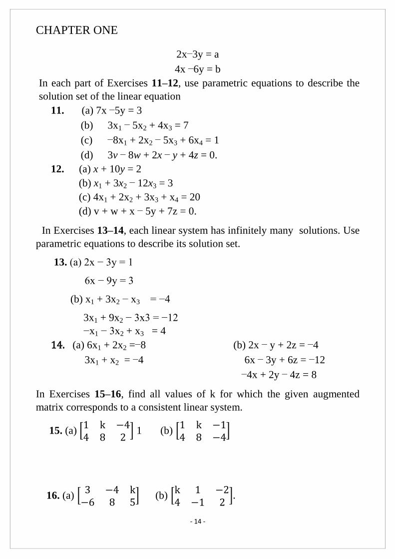
10. Under what conditions on a and b will the following linear system
have no solutions, one solution, and infinitely many solutions?
CHAPTER ONE
- 14 -
2x−3y = a
4x −6y = b
In each part of Exercises 11–12, use parametric equations to describe the
solution set of the linear equation
11. (a) 7x −5y = 3
(b) 3x1 − 5x2 + 4x3 = 7
(c) −8x1 + 2x2 − 5x3 + 6x4 = 1
(d) 3v − 8w + 2x − y + 4z = 0.
12. (a) x + 10y = 2
(b) x1 + 3x2 − 12x3 = 3
(c) 4x1 + 2x2 + 3x3 + x4 = 20
(d) v + w + x − 5y + 7z = 0.
In Exercises 13–14, each linear system has infinitely many solutions. Use
parametric equations to describe its solution set.
13. (a) 2x − 3y = 1
6x − 9y = 3
(b) x1 + 3x2 − x3 = −4
3x1 + 9x2 − 3x3 = −12
−x1 − 3x2 + x3 = 4
14. (a) 6x1 + 2x2 =−8 (b) 2x − y + 2z = −4
3x1 + x2 = −4 6x − 3y + 6z = −12
−4x + 2y − 4z = 8
In Exercises 15–16, find all values of k for which the given augmented
matrix corresponds to a consistent linear system.
15. (a) [1 k −44 8 2
] 1 (b) [1 k −14 8 −4
]
16. (a) [3 −4 k−6 8 5
] (b) [k 1 −24 −1 2
].

CHAPTER ONE
- 15 -
In Exercises, 17–18, find a single elementary row operation that will create
a 1 in the upper left corner of the given augmented matrix and will not
create any fractions in its first row.
17. (a) [−3 −1 2 42 −3 3 20 2 −3 1
] (b) [0 −1 −5 02 −9 3 21 4 −3 3
]
18. (a) [2 4 −6 87 1 4 3−5 4 2 7
] (b) [7 −4 −2 23 −1 8 1−6 3 −1 4
]
CHAPTER ONE
- 16 -
1.2 Gaussian Elimination
DEFINITION 1 If a linear system has infinitely many solutions, then a set
of parametric equations from which all solutions can be obtained by
assigning numerical values to the parameters is called a general solution of
the system.
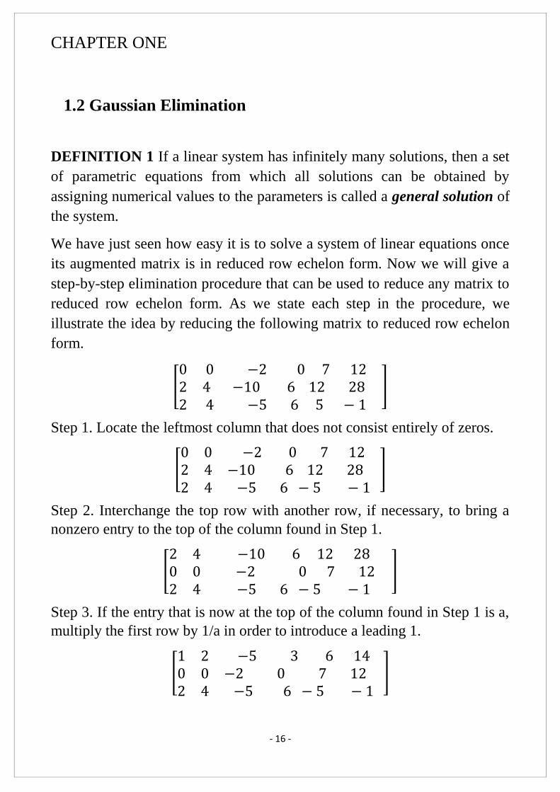
We have just seen how easy it is to solve a system of linear equations once
its augmented matrix is in reduced row echelon form. Now we will give a
step-by-step elimination procedure that can be used to reduce any matrix to
reduced row echelon form. As we state each step in the procedure, we
illustrate the idea by reducing the following matrix to reduced row echelon
form.
[0 0 −2 0 7 122 4 −10 6 12 28 2 4 −5 6 5 − 1
]
Step 1. Locate the leftmost column that does not consist entirely of zeros.
[0 0 −2 0 7 122 4 −10 6 12 28 2 4 −5 6 − 5 − 1
]
Step 2. Interchange the top row with another row, if necessary, to bring a
nonzero entry to the top of the column found in Step 1.
[2 4 −10 6 12 280 0 −2 0 7 12 2 4 −5 6 − 5 − 1
]
Step 3. If the entry that is now at the top of the column found in Step 1 is a,
multiply the first row by 1/a in order to introduce a leading 1.
[1 2 −5 3 6 140 0 −2 0 7 12 2 4 −5 6 − 5 − 1
]
CHAPTER ONE
- 17 -
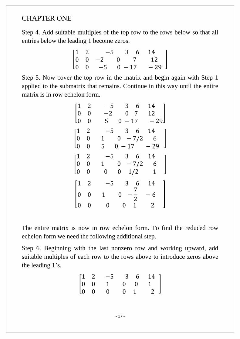
Step 4. Add suitable multiples of the top row to the rows below so that all
entries below the leading 1 become zeros.
[1 2 −5 3 6 140 0 −2 0 7 12 0 0 −5 0 − 17 − 29
]
Step 5. Now cover the top row in the matrix and begin again with Step 1
applied to the submatrix that remains. Continue in this way until the entire
matrix is in row echelon form.
[1 2 −5 3 6 140 0 −2 0 7 12 0 0 5 0 − 17 − 29
]
[1 2 −5 3 6 140 0 1 0 − 7/2 6 0 0 5 0 − 17 − 29
]
[1 2 −5 3 6 140 0 1 0 − 7/2 6 0 0 0 0 1/2 1
]
[
1 2 −5 3 6 14
0 0 1 0 −7
2 − 6
0 0 0 0 1 2
]
The entire matrix is now in row echelon form. To find the reduced row
echelon form we need the following additional step.
Step 6. Beginning with the last nonzero row and working upward, add
suitable multiples of each row to the rows above to introduce zeros above
the leading 1’s.
[1 2 −5 3 6 140 0 1 0 0 1 0 0 0 0 1 2
]
CHAPTER ONE
- 18 -
[1 2 −5 3 0 20 0 1 0 0 1 0 0 0 0 1 2
]
[1 2 0 3 0 70 0 1 0 0 1 0 0 0 0 1 2
]
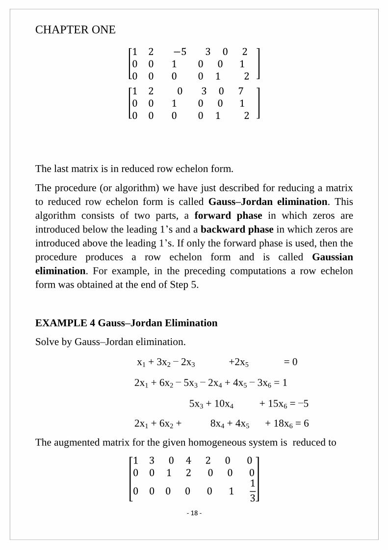
The last matrix is in reduced row echelon form.
The procedure (or algorithm) we have just described for reducing a matrix
to reduced row echelon form is called Gauss–Jordan elimination. This
algorithm consists of two parts, a forward phase in which zeros are
introduced below the leading 1’s and a backward phase in which zeros are
introduced above the leading 1’s. If only the forward phase is used, then the
procedure produces a row echelon form and is called Gaussian
elimination. For example, in the preceding computations a row echelon
form was obtained at the end of Step 5.
EXAMPLE 4 Gauss–Jordan Elimination
Solve by Gauss–Jordan elimination.
x1 + 3x2 − 2x3 +2x5 = 0
2x1 + 6x2 − 5x3 − 2x4 + 4x5 − 3x6 = 1
5x3 + 10x4 + 15x6 = −5
2x1 + 6x2 + 8x4 + 4x5 + 18x6 = 6
The augmented matrix for the given homogeneous system is reduced to
[
1 3 0 4 2 0 00 0 1 2 0 0 0
0 0 0 0 0 1 1
3
]
CHAPTER ONE
- 19 -
The corresponding system of equations is
x1 + 3x2 + 4x4 + 2x5 = 0
x3 + 2x4 = 0
x6 = 1/3
Solving for the leading variables, we obtain
x1 = −3x2 − 4x4 − 2x5
x3 = −2x4
x6 = 1/3.
Finally, we express the general solution of the system Parametrically by
assigning the free variables x2, x4, and x5 arbitrary values r, s, and t,
respectively. This yield
x1 = −3r − 4s − 2t, x2 = r, x3 = −2s, x4 = s, x5 = t, x6 = 1/3.
EXAMPLE 5 A Homogeneous System
Use Gauss–Jordan elimination to solve the homogeneous linear system
x1 + 3x2 − 2x3 +2x5 = 0
2x1 + 6x2 − 5x3 − 2x4 + 4x5 − 3x6 = 0
5x3 + 10x4 + 15x6 = 0
2x1 + 6x2 + 8x4 + 4x5 + 18x6 = 0
The augmented matrix for the given homogeneous system is reduced to
[1 3 0 4 2 0 00 0 1 2 0 0 00 0 0 0 0 1 0
]
The corresponding system of equations is
CHAPTER ONE
- 20 -
x1 + 3x2 + 4x4 + 2x5 = 0
x3 + 2x4 = 0
x6 = 0
Solving for the leading variables, we obtain
x1 = −3x2 − 4x4 − 2x5
x3 = −2x4
x6 = 0.
If we now assign the free variables x2, x4, and x5 arbitrary values r, s, and t,
respectively, then we can express the solution set parametrically as
x1 = −3r − 4s − 2t, x2 = r, x3 = −2s, x4 = s, x5 = t, x6 = 0
Note that the trivial solution results when r = s = t = 0.
CHAPTER ONE
- 21 -
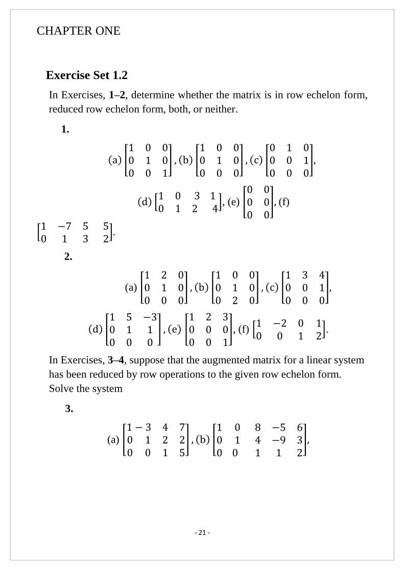
Exercise Set 1.2
In Exercises, 1–2, determine whether the matrix is in row echelon form,
reduced row echelon form, both, or neither.
1.
(a) [1 0 00 1 00 0 1
] , (b) [1 0 00 1 00 0 0
] , (c) [0 1 00 0 10 0 0
],
(d) [1 0 3 10 1 2 4
], (e) [0 00 00 0
], (f)
[1 −7 5 50 1 3 2
].
2.
(a) [1 2 00 1 00 0 0
] , (b) [1 0 00 1 00 2 0
] , (c) [1 3 40 0 10 0 0
],
(d) [1 5 −30 1 10 0 0
] , (e) [1 2 30 0 00 0 1
], (f) [1 −2 0 10 0 1 2
].
In Exercises, 3–4, suppose that the augmented matrix for a linear system
has been reduced by row operations to the given row echelon form.
Solve the system
3.
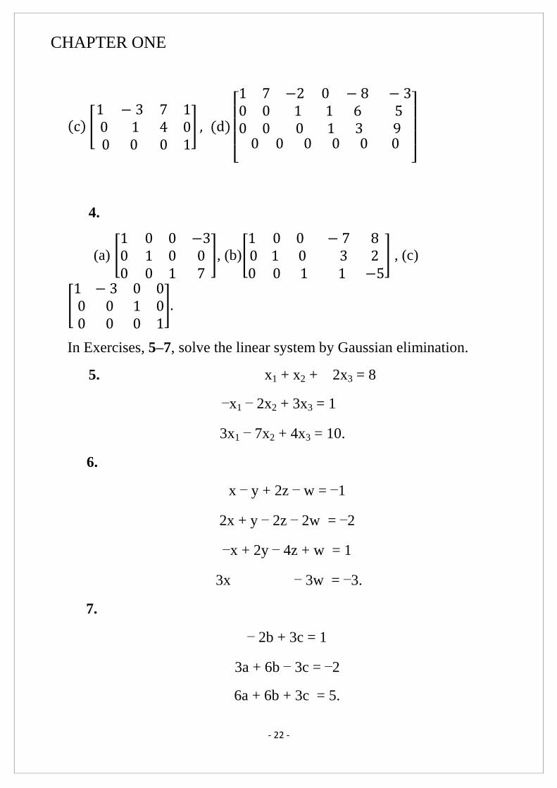
(a) [1 − 3 4 70 1 2 20 0 1 5
] , (b) [1 0 8 −5 60 1 4 −9 30 0 1 1 2
],
CHAPTER ONE
- 22 -
(c) [1 − 3 7 10 1 4 0 0 0 0 1
] , (d)
[ 1 7 −2 0 − 8 − 30 0 1 1 6 50 0 0 1 3 90 0 0 0 0 0
]
4.
(a) [1 0 0 −30 1 0 00 0 1 7
], (b)[1 0 0 − 7 80 1 0 3 20 0 1 1 −5
] , (c)
[1 − 3 0 00 0 1 00 0 0 1
].
In Exercises, 5–7, solve the linear system by Gaussian elimination.
5. x1 + x2 + 2x3 = 8
−x1 − 2x2 + 3x3 = 1
3x1 − 7x2 + 4x3 = 10.
6.
x − y + 2z − w = −1
2x + y − 2z − 2w = −2
−x + 2y − 4z + w = 1
3x − 3w = −3.
7.
− 2b + 3c = 1
3a + 6b − 3c = −2
6a + 6b + 3c = 5.
CHAPTER ONE
- 23 -
In Exercises, 8–10, solve the linear system by Gauss–Jordan
elimination.
8. Exercise 5 9. Exercise 6 10. Exercise 7
In Exercises, 11–12, determine whether the homogeneous system
has nontrivial solutions by inspection (without pencil and paper).
11. 2x1 − 3x2 + 4x3 − x4 = 0
7x1 + x2 − 8x3 + 9x4 = 0
2x1 + 8x2 + x3 − x4 = 0
12. x1 + 3x2 − x3 = 0
x2 − 8x3 = 0
4x3 = 0
In Exercises, 13–17, solve the given linear system by any method.
13. 2x1 + x2 + 3x3 = 0
x1 + 2x2 = 0
x2 + x3 = 0.
14. 2x − y − 3z = 0
−x + 2y − 3z = 0
x + y + 4z = 0.
15. 3x1 + x2 + x3 + x4 = 0
5x1 − x2 + x3 − x4 = 0.
16. v + 3w − 2x = 0
2u + v − 4w + 3x = 0
2u + 3v + 2w − x = 0

CHAPTER ONE
- 24 -
−4u − 3v + 5w − 4x = 0.
17. 2x + 2y + 4z = 0
w − y − 3z = 0
2w + 3x + y + z = 0
−2w + x + 3y − 2z = 0.
In Exercises, 18–19, determine the values of a for which the system has no
solutions, exactly one solution, or infinitely many solutions
18. x + 2y − 3z = 4
3x − y + 5z = 2
4x + y + (a2 − 14) z = a + 2.
19. x + 2y + z = 2
2x − 2y + 3z = 1
x + 2y − (a2 – 3) z = a.
In Exercises, 20-21, solve the following systems, where a, b, and c are
constants
20.
2x + y = a
3x + 6y = b.
21.
x1 + x2 + x3 = a
2x1 + 2x3 = b
3x2 + 3x3 = c.
In Exercises, 22–23, what condition, if any, must a, b, and c satisfy for the
linear system to be consistent

CHAPTER ONE
- 25 -
22. x + 3y − z = a
x + y + 2z = b
2y − 3z = c.
23. x + 3y + z = a
−x − 2y + z = b
3x + 7y − z = c.
24. Solve the following system of nonlinear equations for x, y, and z.
x2 + y
2 + z
2 = 6
x2 − y
2 + 2z
2 = 2
2x2 + y
2 − z
2 = 3
25. Solve the following system for x, y, and z.
1/x + 2/y− 4/z = 1
2/x + 3/y + 8/z = 0
−1/x + 9/y + 10/z = 5

CHAPTER ONE
- 26 -
1.3 Matrices and Matrix Operations
DEFINITION 1 A matrix is a rectangular array of numbers. The numbers in
the array are called the entries in the matrix.
EXAMPLE 1 Examples of Matrices
Some examples of matrices are
[1 23 0−1 4
], [2 1 0], [e π −√20 1/2 10 0 0
], [13], [4].
The size of a matrix is described in terms of the number of rows (horizontal
lines) and columns (vertical lines) it contains. For example, the first matrix
in Example 1 has three rows and two columns, so its size is 3 by 2 (written
3 × 2). In a size description, the first number always denotes the number of
rows, and the second denotes the number of columns. The remaining
matrices in Example 1 have sizes 1 × 4, 3 × 3, 2 × 1, and 1 × 1,
respectively.
A matrix with only one row, such as the second in Example 1, is called a
row vector (or a row matrix), and a matrix with only one column, such as
the fourth in that example, is called a column vector (or a column matrix).
The fifth matrix in that example is both a row vector and a column vector.
We will use capital letters to denote matrices and lowercase letters to
denote numerical quantities; thus, we might write
A = [2 1 73 4 2
], or C = [a b cd e f
].
The entry that occurs in row i and column j of a matrix A will be denoted
by aJJ.

CHAPTER ONE
- 27 -
Thus, a general 3 × 4 matrix might be written as
A = [
a11 a12 a13 a14a21 a22 a23 a24a31 a32 a33 a34
],
and a general m × n matrix as
A = [
a11 a12… a1na21 a22… a2n
am1 am2 amn
].
When a compact notation is desired, the preceding matrix can be written as
[aij]m×n or [aij],
the first notation being used when it is important in the discussion to know
the size, and the second when the size need not be emphasized. Usually, we
will match the letter denoting a matrix with the letter denoting its entries;
thus, for a matrix B we would generally use bij for the entry in row i and
column j , and for a matrix C we would use the notation cij.
The entry in row i and column j of a matrix A is also commonly denoted by
the symbol (A)ij. Thus, for matrix (1) above, we have
(A)ij = aij,
and for the matrix
A = [2 −37 0
],
we have (A)11 = 2, (A)12 = −3, (A)21 = 7, and (A)22 = 0.
Row and column vectors are of special importance, and it is common
practice to denote them by boldface lowercase letters rather than capital
letters. For such matrices, double subscripting of the entries is unnecessary.
Thus a general 1 × n row vector a and a general m × 1 column vector b
would be written as
CHAPTER ONE
- 28 -
[a1 a2 an],
[ b1b2
bm]
.
A matrix A with n rows and n columns is called a square matrix of order
n.
[ a11 a12 a1na21 a22 a2n
an1 an2 ann]
DEFINITION 2 Two matrices are defined to be equal if they have the
same size and their corresponding entries are equal.
EXAMPLE 2 Equality of Matrices
Consider the matrices
A = [2 13 x
] , B = [2 13 5
] , C = [2 1 03 4 0
].
If x = 5, then A = B, but for all other values of x the matrices A and B are
not equal, since not all of their corresponding entries are equal. There is no
value of x for which A = C since A and C have different sizes.
DEFINITION 3 If A and B are matrices of the same size, then the sum A
+ B is the matrix obtained by adding the entries of B to the corresponding
entries of A, and the difference A − B is the matrix obtained by subtracting
the entries of B from the corresponding entries of A. Matrices of different
sizes cannot be added or subtracted.

CHAPTER ONE
- 29 -
EXAMPLE 3 Addition and Subtraction
Consider the matrices
A = [2 1 0 3−1 0 2 44 −2 7 0
], B = [−4 3 5 12 2 0 − 13 2 −4 5
], C = [1 12 2
].
Then
A + B = [−2 4 5 41 2 2 37 0 3 5
], A – B = [6 −2 −5 2−3 −2 2 51 −4 11 − 5
].
The expressions A + C, B + C, A − C, and B − C are undefined.
DEFINITION 4 If A is any matrix and c is any scalar, then the product
cA is the matrix obtained by multiplying each entry of the matrix A by c.
The matrix cA is said to be a scalar multiple of A.
In matrix notation, if A = [aij ], then
(cA)ij = c(A)ij = caij
EXAMPLE 4 Scalar Multiples
For the matrices
A = [2 3 41 3 1
] , B = [0 2 7−1 3 −5
] , C = [9 −6 33 0 12
],
we have
2A = [4 6 82 6 2
] , (−1)B = [0 −2 −71 −3 5
] ,1
3 C = [
3 −2 11 0 4
].
It is common practice to denote (−1)B by −B.

CHAPTER ONE
- 30 -
DEFINITION 5 If A is an m × r matrix and B is an r × n matrix, then the
product AB is the m × n matrix whose entries are determined as follows:
To find the entry in row i and column j of AB, single out row i from the
matrix A and column j from the matrix B. Multiply the corresponding
entries from the row and column together, and then add up the resulting
products.
EXAMPLE 5 Multiplying Matrices
Consider the matrices
A = [1 2 42 6 0
], B = [4 1 4 30 −1 3 12 7 5 2
].
Since A is a 2 × 3 matrix and B is a 3 × 4 matrix, the product AB is a 2×
4 matrix. To determine, for example, the entry in row 2 and column 3 of
AB, we single out row 2 from A and column 3 from B. Then, as illustrated
below, we multiply corresponding entries together and add up these
products.
[1 2 42 6 0
] [4 1 4 30 −1 3 12 7 5 2
] = [26 ]
(2 · 4) + (6 · 3) + (0 · 5) = 26.
The entry in row 1 and column 4 of AB is computed as follows
[1 2 42 6 0
] [4 1 4 30 −1 3 12 7 5 2
] = [ 13]
(1 · 3) + (2 · 1) + (4 · 2) = 13.
The computations for the remaining entries are
(1 · 4) + (2 · 0) + (4 · 2) = 12
CHAPTER ONE
- 31 -
(1 · 1) − (2 · 1) + (4 · 7) = 27
(1 · 4) + (2 · 3) + (4 · 5) = 30 AB =[12 27 308 −4 26
1312].
(2 · 4) + (6 · 0) + (0 · 2) = 8
(2 · 1) − (6 · 1) + (0 · 7) = −4
(2 · 3) + (6 · 1) + (0 · 2) = 12
The definition of matrix multiplication requires that the number of columns
of the first factor A be the same as the number of rows of the second factor
B in order to form the product AB. If this condition is not satisfied, the
product is undefined. A convenient way to determine whether a product of
two matrices is defined is to write down the size of the first factor and, to
the right of it, write down the size of the second factor.
If the inside numbers are the same, then the product is defined. The outside
numbers then give the size of the product.
A B AB
m × r r × n m × n
EXAMPLE 6 Determining Whether a Product Is Defined
Suppose that A, B, and C are matrices with the following sizes:
A B C
3 ×4 4×7 7× 3
Then AB is defined and is a 3 × 7 matrix; BC is defined and is a 4 × 3
matrix; and CA is defined and is a 7 × 4 matrix. The products AC, CB,
and BA are all undefined.

CHAPTER ONE
- 32 -
DEFINITION 6 If A1, A2, . . . , Ar are matrices of the same size, and if c1,
c2, . . . , cr are scalars, then an expression of the form c1A1 + c2A2 +· · ·
+crAr is called a linear combination of A1, A2, . . . , Ar with coefficients c1,
c2, . . . , cr.
Matrix multiplication has an important application to systems of linear
equations. Consider a system of m linear equations in n unknowns:
a11x1 + a12x2 + · · · + a1nxn = b1
a21x1 + a22x2 + · · · + a2nxn = b2
...
...
...
am1x1 + am2x2 + · · · + amnxn = bm
Since two matrices are equal if and only if their corresponding entries are
equal, we can replace the m equations in this system by the single matrix
equation
[
a11x1 + a12x2 +⋯+ a1nxna21x1 + a22x2 +⋯+ a2nxn
am1x1 + am2x2 +⋯+ amnxn
] =
[ b1b2
bm]
.
The m × 1 matrix on the left side of this equation can be written as a
product to give
[
a11 a12 … a1na21 a22 … a2n
am1 am2 … amn
] [
x1x 2
xm
] =
[ b1b2
bm]
.
If we designate these matrices by A, x, and b, respectively, then we can
replace the original system of m equations in n unknowns by the single
matrix equation
CHAPTER ONE
- 33 -
Ax = b.
The matrix A in this equation is called the coefficient matrix of the system.
The augmented matrix for the system is obtained by adjoining b to A as the
last column; thus the augmented matrix [A | b] is
[A | b] =
[ a11 a12 … a1n | b1 a21 a22 … a2n |b2
am1 am2 … amn |bm ]
.
We conclude this section by defining two matrix operations that have no
analogs in the arithmetic of real numbers.
DEFINITION 7 If A is any m × n matrix, then the transpose of A,
denoted by AT, is defined to be the n × m matrix that results by
interchanging the rows and columns of A; that is, the first column of AT is
the first row of A, the second column of AT is the second row of A, and so
forth.
EXAMPLE 7 Some Transposes
The following are some examples of matrices and their transposes.
A = [
a11 a12 a13 a21 a22 a23 a31 a32 a33
] , B = [2 31 45 6
] , C = [1 3 5], D = [4]
AT = [
a11 a21 a31a12 a22 a32 a13 a23 a33
], BT = [2 1 53 4 6
] , CT = [135] , DT = [4].

CHAPTER ONE
- 34 -
DEFINITION 8 If A is a square matrix, then the trace of A, denoted by tr
(A), is defined to be the sum of the entries on the main diagonal of A. The
trace of A is undefined if A is not a square matrix.
EXAMPLE 8 Trace
The following are examples of matrices and their traces
A = [
a11 a12 a13a21 a22 a23a31 a32 a33
] , B = [
−1 2 7 03 5 −8 41 2 7 − 34 −2 1 0
],
Tr (A) = a11 + a22 + a33, Tr (B) = −1 +5 +7 + 0 = 11.

CHAPTER ONE
- 35 -
Exercise set 1.3
In Exercises, 1–2, suppose that A, B, C, D, and E are matrices with the
following sizes:
A B C D E
(4 × 5) (4 × 5) (5 × 2) (4 × 2) (5 × 4)
In each part, determine whether the given matrix expression is defined. For
those that are defined, give the size of the resulting matrix
1. (a) BA (b) ABT (c) AC + D (d) E(AC) (e) A − 3E
T (f) E(5B +
A)
2. (a) CDT (b) DC (c) BC − 3D (d) DT (BE) (e) B
TD + ED (f) BA
T + D
In Exercises, 3–6, use the following matrices to compute the indicated
expression if it is defined.
A = [3 0−1 21 1
] , B = [4 −10 2
] , C = [1 4 23 1 5
]
D = [1 5 2−1 0 13 2 4
] , E = [6 1 3−1 1 24 1 3
]
3. (a) D + E (b) D − E (c) 5A (d) −7C (e) 2B − C (f) 4E − 2D
(g) −3(D + 2E) (h) A – A (i) tr(D) ( j) tr(D − 3E) (k) 4 tr(7B) (l) tr(A)
4. (a) 2AT + C (b) D
T − E
T (c) (D − E)
T (d) B
T + 5C
T (e) 1/2C
T – 1/4A
(f) B − BT
(g) 2ET − 3D
T (h) (2E
T − 3D
T )
T (i) (CD)E (j) C(BA)
(k) tr(DET) (l) tr(BC)
5. (a) AB (b) BA (c) (3E)D (d) (AB)C (e) A(BC) (f ) CCT

CHAPTER ONE
- 36 -
(g) (DA)T (h) (C
TB)A
T (i) tr(DD
T ) ( j) tr(4E
T−D) (k) tr(CTA
T + 2E
T ) (l)
tr((ECT )
TA)
6. (a) (2DT − E)A (b) (4B)C + 2B (c) (−AC)
T + 5D
T (d) (BA
T − 2C)
T (e)
BT(CC
T − A
TA) (f) D
TE
T − (ED)
In each part of Exercises, 7–8, find matrices A, x, and b that express the
given linear system as a single matrix equation Ax = b, and write out this
matrix equation.
7. (a) 2x1 − 3x2 + 5x3 = 7
9x1 − x2 + x3 = −1
x1 + 5x2 + 4x3 = 0
(b) 4x1 − 3x3 + x4 = 1
5x1 + x2 − 8x4 = 3
2x1−5x2 + 9x3 − x4 = 0
3x2 − x3 + 7x4 = 2
8. (a) x1 − 2x2 + 3x3 = −3
2x1 + x2 = 0
− 3x2 + 4x3 = 1
x1 + x3 = 5
(b) 3x1 + 3x2 + 3x3 = −3
−x1−5x2−2x3 = 3
− 4x2 + x3 = 0

CHAPTER ONE
- 37 -
In each part of Exercises, 9–10, express the matrix equation as a system of
linear equations,
9. a) [5 6 −7−1 −2 30 4 −1
] [
x1x2x3] = [
203]
b) [1 1 12 3 05 −3 −6
] [xyz] = [
22−9]
10. a) [3 −1 24 3 7−2 1 5
] [
x1x2x3] = [
2−14]
b) [
3 − 2 0 15 0 2 − 23 1 4 7−2 5 1 6
] [
wxyz
] = [
0000
]
In Exercises, 11–12, find all values of k, if any, that satisfy the equation.
11. [k 1 1] [1 1 01 0 20 2 −3
] [k11] = 0
12. [2 2 k] [1 2 02 0 30 3 1
] [22k] = 0
In Exercises 13–14, solve the matrix equation for a, b, c, and d.
13. [a 3−1 a + b
] = [4 d − 2c
d + 2c −2]
14. [a − b b + a3d + c 2d − c
] = [8 17 6
]
15. A matrix B is said to be a square root of a matrix A if BB = A.

CHAPTER ONE
- 38 -
(a) Find two square roots of A = [2 22 2
].
CHAPTER ONE
- 39 -
1.4 Inverses; Algebraic Properties of Matrices
The following theorem lists the basic algebraic properties of the matrix
operations.
THEOREM 1.4.1 Properties of Matrix Arithmetic
Assuming that the sizes of the matrices are such that the indicated
operations can be performed, the following rules of matrix arithmetic are
valid.
(a) A + B = B + A [Commutative law for matrix addition]
(b) A + (B + C) = (A + B) + C [Associative law for matrix addition]
(c) A(BC) = (AB)C [Associative law for matrix multiplication]
(d ) A(B + C) = AB + AC [Left distributive law]
(e) (B + C)A = BA + CA [Right distributive law]
(f) A(B − C) = AB − AC
(g) (B − C)A = BA − CA
(h) a(B + C) = a B + a C
(i) a(B − C) = a B – a C
(j) (a + b)C = a C + b C
(k) (a − b)C = a C – b C
(l) a(b C) = (ab)C
(m) a(BC) = (a B)C = B(a C).
EXAMPLE 1 Associativity of Matrix Multiplication
As an illustration of the associative law for matrix multiplication, consider

CHAPTER ONE
- 40 -
A = [1 23 40 1
], B = [4 32 1
], C = [1 02 3
]
Then
AB = [1 23 40 1
] [4 32 1
] = [8 520 132 1
],
and BC = [4 32 1
] [1 02 3
] = [10 94 3
].
Thus (AB)C = [8 520 132 1
] [1 02 3
] =[18 1546 394 3
],
and A (BC) = [1 23 40 1
] [10 94 3
] = [18 1546 394 3
],
so (AB)C = A(BC), as guaranteed by Theorem 1.4.1(c).
Do not let Theorem 1.4.1 full you into believing that all laws of real
arithmetic carry over to matrix arithmetic. For example, you know that in
real arithmetic it is always true that ab = ba, which is called the
commutative law for multiplication. In matrix arithmetic, however, the
equality of AB and BA can fail for three possible reasons:
1. AB may be defined and BA may not (for example, if A is 2 × 3 and B is
3 × 4).
2. AB and BA may both be defined, but they may have different sizes (for
example, if A is 2 × 3 and B is 3 × 2).
3. AB and BA may both be defined and have the same size, but the two
products may be different (as illustrated in the next example).

CHAPTER ONE
- 41 -
EXAMPLE 2 Order Matters in Matrix Multiplication
Consider the matrices
A = [−1 02 3
], B = [1 23 0
]
Multiplying gives
AB = [−1 −211 4
] and BA = [3 6−3 0
].
Thus AB ≠ 𝐵𝐴.
Zero Matrices A matrix whose entries are all zero is called a zero matrix.
Some examples are
[0 00 0
] , [0 0 00 0 00 0 0
] , [0 0 00 0 0
], [0 00 00 0
], [0].
We will denote a zero matrix by 0 unless it is important to specify its size,
in which case we will denote the m × n zero matrix by 0m×n.
It should be evident that if A and 0 are matrices with the same size, then
A + 0 = 0 + A = A
Thus, 0 plays the same role in this matrix equation that the number 0 plays
in the numerical equation a + 0 = 0 + a = a.
The following theorem lists the basic properties of zero matrices. Since the
results should be self-evident, we will omit the formal proofs.
THEOREM 1.4.2 Properties of Zero Matrices

CHAPTER ONE
- 42 -
If c is a scalar, and if the sizes of the matrices are such that the operations
can be performed, then:
(a) A + 0 = 0 + A = A
(b) A − 0 = A
(c) A − A = A + (−A) = 0
(d) 0A = 0
(e) If c A = 0, then c = 0 or A = 0.
EXAMPLE 3 Failure of the Cancellation Law
Consider the matrices
A = [0 10 2
], B = [1 13 4
], C = [2 53 4
].
It is easy to show that
𝐴𝐵 = 𝐴𝐶 = [3 46 8
] .
Although A ≠ 0, canceling A from both sides of the equation AB = AC
would lead to the incorrect conclusion that B = C. Thus, the cancellation
law does not hold, in general, for matrix multiplication (though there may
be particular cases where it is true).
EXAMPLE 4 A Zero Product with Nonzero Factors
Here are two matrices for which AB = 0, but A≠0 and B≠ 0
A = [0 10 2
], B = [3 70 0
].
A square matrix with 1’s on the main diagonal and zeros elsewhere is
called an identity matrix. Some examples are

CHAPTER ONE
- 43 -
[1], [1 00 1
], [1 0 00 1 00 0 1
].
An identity matrix is denoted by the letter I . If it is important to emphasize
the size, we will write In for the n × n identity matrix.
To explain the role of identity matrices in matrix arithmetic, let us consider
the effect of multiplying a general 2 × 3 matrix A on each side by an
identity matrix. Multiplying on the right by the 3 × 3 identity matrix yields
AI3 = [𝑎11 𝑎12 𝑎13𝑎21 𝑎22 𝑎23
] [1 0 00 1 00 0 1
] = [𝑎11 𝑎12 𝑎13𝑎21 𝑎22 𝑎23
] = A
I2 A = [1 00 1
] [𝑎11 𝑎12 𝑎13𝑎21 𝑎22 𝑎23
] = [𝑎11 𝑎12 𝑎13𝑎21 𝑎22 𝑎23
] = A
The same result holds in general; that is, if A is any m × n matrix, then A In
= A and Im A = A. Thus, the identity matrices play the same role in matrix
arithmetic that the number 1plays in the numerical equation a · 1 = 1 · a =
a. As the next theorem shows, identity matrices arise naturally in studying
reduced row echelon forms of square matrices.
THEOREM 1,4.3 If R is the reduced row echelon form of an n × n matrix
A, then either R has a row of zeros or R is the identity matrix In.
Inverse of a Matrix In real arithmetic every nonzero number a has a
reciprocal a-1
(= 1/a) with the property a · a-1
= a-1
· a = 1. The number a-1
is sometimes called the multiplicative inverse of a. Our next objective is to
develop an analog of this result for matrix arithmetic. For this purpose we
make the following definition.

CHAPTER ONE
- 44 -
DEFINITION 1 If A is a square matrix, and if a matrix B of the same size
can be found such that AB = BA = I , then A is said to be invertible (or
nonsingular) and B is called an inverse of A. If no such matrix B can be
found, then A is said to be singular.
EXAMPLE 5 An Invertible Matrix
Let
A = [2 −5−1 3
] , and B = [3 51 2
]
Then
AB = [2 −5−1 3
] [3 51 2
] = [1 00 1
] = I
BA = [3 51 2
] [2 −5−1 3
] = [1 00 1
] = I
Thus, A and B are invertible and each is an inverse of the other
EXAMPLE 6 A Class of Singular Matrices
A square matrix with a row or column of zeros is singular. To help
understand why this is so, consider the matrix
A = [1 4 02 5 03 6 0
].
To prove that A is singular we must show that there is no 3 × 3 matrix B
such that AB = BA = I. For this purpose let c1, c2, 0 be the column vectors
of A. Thus, for any 3 × 3 matrix B we can express the product BA as
BA = B [𝑐1 𝑐2 0] = [𝐵𝑐1 𝐵𝑐2 0]
The column of zeros shows that BA ≠ I and hence that A is singular

CHAPTER ONE
- 45 -
It is reasonable to ask whether an invertible matrix can have more than one
inverse. The next theorem shows that the answer is no—an invertible
matrix has exactly one inverse.
THEOREM 1.4.4 If B and C are both inverses of the matrix A,
then B = C.
Proof Since B is an inverse of A, we have BA = I. Multiplying both sides
on the right by C gives (BA)C = IC = C. But it is also true that (BA)C =
B(AC) = BI = B, so C = B.
As a consequence of this important result, we can now speak of “the”
inverse of an invertible matrix. If A is invertible, then its inverse will be
denoted by the symbol A-1
.
Thus,
AA-1
= I and A-1
A = I 1)
The inverse of A plays much the same role in matrix arithmetic that the
reciprocal a-1
plays in the numerical relationships aa-1
= 1 and a-1
a = 1.
In the next section we will develop a method for computing the inverse of
an invertible matrix of any size. For now we give the following theorem
that specifies conditions under which a 2 × 2 matrix is invertible and
provides a simple formula for its inverse.
THEOREM 1.4.5 The matrix
A = [𝑎 𝑏𝑐 𝑑
],
is invertible if and only if ad-bc≠ 0 in which case the inverse is given by
the formula
A-1
= 1
𝑎𝑑−𝑏𝑐 [𝑑 −𝑏−𝑐 𝑎
]. 2)

CHAPTER ONE
- 46 -
EXAMPLE 7 Calculating the Inverse of a 2 × 2 Matrix
In each part, determine whether the matrix is invertible. If so, find its
inverse.
(a) A = [6 15 2
], (b) A = [−1 23 −6
].
Solution (a) The determinant of A is det(A) = (6)(2) − (1)(5) = 7, which is
nonzero. Thus, A is invertible, and its inverse is
A-1
= 1
7 [2 −1−5 6
] = [2/7 −1/7−5/7 6/7
]
Solution (b) The matrix is not invertible since det(A) = (−1)(−6) − (2)(3) =
0
EXAMPLE 8 Solution of a Linear System by Matrix Inversion
A problem that arises in many applications is to solve a pair of equations of
the form
u = ax + by
v = cx + dy
for x and y in terms of u and v. One approach is to treat this as a linear
system of two equations in the unknowns x and y and use Gauss–Jordan
elimination to solve for x and y. However, because the coefficients of the
unknowns are literal rather than numerical, this procedure is a little clumsy.
As an alternative approach, let us replace the two equations by the single
matrix equation
CHAPTER ONE
- 47 -
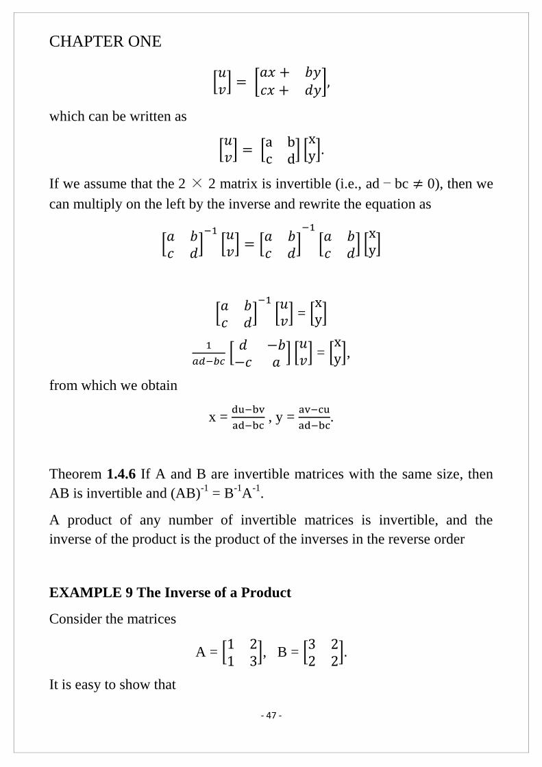
[𝑢𝑣] = [
𝑎𝑥 + 𝑏𝑦𝑐𝑥 + 𝑑𝑦
],
which can be written as
[𝑢𝑣] = [
a bc d
] [xy].
If we assume that the 2 × 2 matrix is invertible (i.e., ad − bc ≠ 0), then we
can multiply on the left by the inverse and rewrite the equation as
[𝑎 𝑏𝑐 𝑑
]−1
[𝑢𝑣] = [
𝑎 𝑏𝑐 𝑑
]−1
[𝑎 𝑏𝑐 𝑑
] [xy]
[𝑎 𝑏𝑐 𝑑
]−1
[𝑢𝑣] = [
xy]
1
𝑎𝑑−𝑏𝑐 [𝑑 −𝑏−𝑐 𝑎
] [𝑢𝑣] = [
xy],
from which we obtain
x = du−bv
ad−bc , y =
av−cu
ad−bc.
Theorem 1.4.6 If A and B are invertible matrices with the same size, then
AB is invertible and (AB)-1
= B-1
A-1
.
A product of any number of invertible matrices is invertible, and the
inverse of the product is the product of the inverses in the reverse order
EXAMPLE 9 The Inverse of a Product
Consider the matrices
A = [1 21 3
], B = [3 22 2
].
It is easy to show that

CHAPTER ONE
- 48 -
AB = [7 69 8
], (𝐴𝐵)−1= [4 −3
−9/2 7/2],
and also that
𝐴−1 = [3 −2−1 1
], 𝐵−1 = [1 −1−1 3/2
], 𝐵−1𝐴−1=[1 −1−1 3/2
] [3 −2−1 1
] =
[4 −3
−9/2 7/2]
Thus, 𝐵−1𝐴−1 = (𝐴𝐵)−1, as guaranteed by Theorem 1.4.6.
Powers of a Matrix If A is a square matrix, then we define the nonnegative
integer powers of A to be
𝐴0 = I, An = A.A….A [n factors],
and if A is invertible, then we define the negative integer powers of A to be
A−n = (A−1)n = A−1. A−1…A−1 [n factors].
Because these definitions parallel those for real numbers, the usual laws of
nonnegative exponents hold; for example,
Ar. As = Ar+s , (𝐴𝑟)𝑠 = Ars
In addition, we have the following properties of negative exponents.
THEOREM 1.4.7 If A is invertible and n is a nonnegative integer, then
(a) A-1
is invertible and (A-1
)-1
= A.
(b) An is invertible and (A
n)-1
= A-n
= (A-1
)n.
(c) kA is invertible for any nonzero scalar k, and (kA)-1
= k-1
A-1
.
EXAMPLE 10 Properties of Exponents
CHAPTER ONE
- 49 -
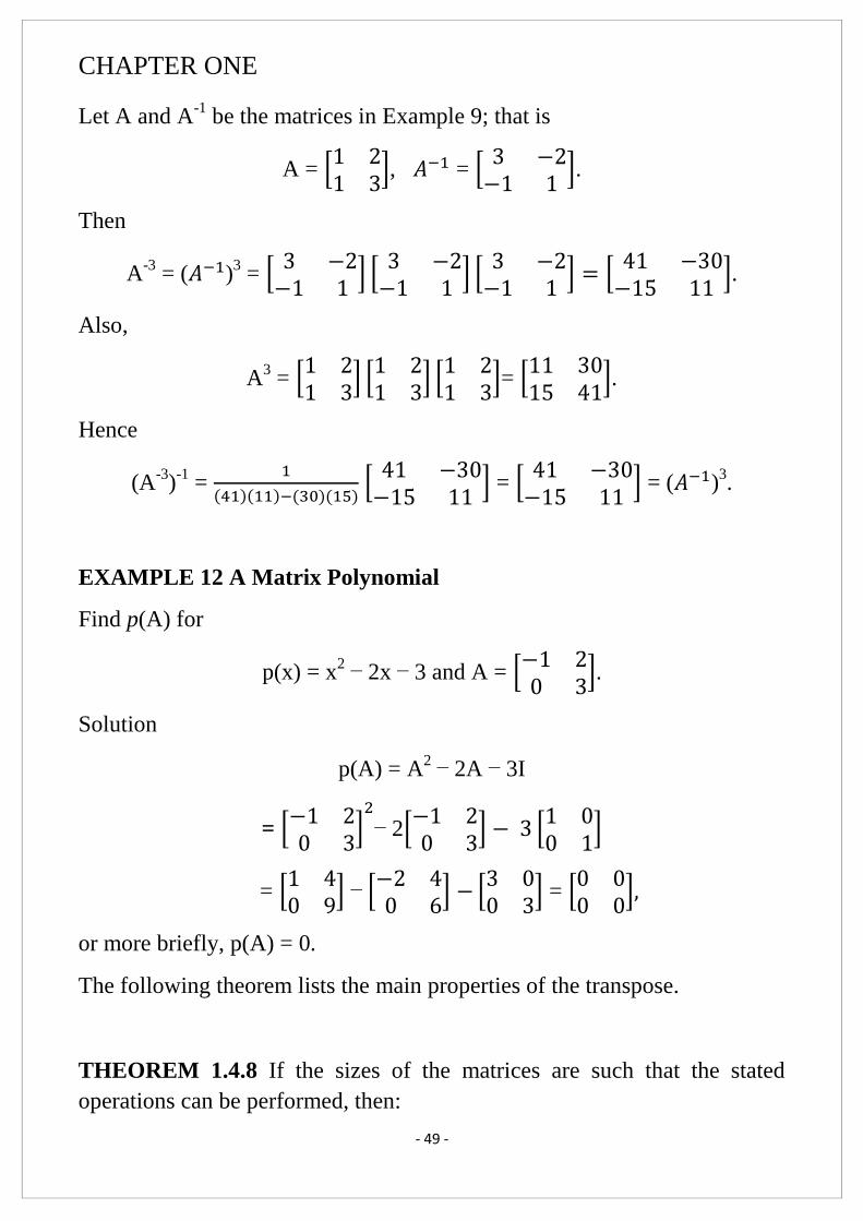
Let A and A-1
be the matrices in Example 9; that is
A = [1 21 3
], 𝐴−1 = [3 −2−1 1
].
Then
A-3
= (𝐴−1)3 = [
3 −2−1 1
] [3 −2−1 1
] [3 −2−1 1
] = [41 −30−15 11
].
Also,
A3 = [1 21 3
] [1 21 3
] [1 21 3
]= [11 3015 41
].
Hence
(A-3
)-1
= 1
(41)(11)−(30)(15) [41 −30−15 11
] = [41 −30−15 11
] = (𝐴−1)3.
EXAMPLE 12 A Matrix Polynomial
Find p(A) for
p(x) = x2 − 2x − 3 and A = [
−1 20 3
].
Solution
p(A) = A2 − 2A − 3I
= [−1 20 3
]2
− 2[−1 20 3
] − 3 [1 00 1
]
= [1 40 9
] − [−2 40 6
] −[3 00 3
] = [0 00 0
],
or more briefly, p(A) = 0.
The following theorem lists the main properties of the transpose.
THEOREM 1.4.8 If the sizes of the matrices are such that the stated
operations can be performed, then:

CHAPTER ONE
- 50 -
(a) (AT )
T = A
(b) (A + B)T = A
T + B
T
(c) (A − B)T = A
T − B
T
(d) (kA)T = k A
T
(e) (AB)T = B
TA
T
THEOREM 1.4.9 If A is an invertible matrix, then AT is also invertible
and (AT )
-1 = (A
-1)
T
EXAMPLE 13 Inverse of a Transpose
Consider a general 2 × 2 invertible matrix and its transpose:
A = [𝑎 𝑏𝑐 𝑑
], AT = [𝑎 𝑐𝑏 𝑑
]
Since A is invertible, its determinant ad − bc is nonzero. But the
determinant of AT is also ad – bc (verify), so A
T is also invertible. It follows
from Theorem 1.4.5 that
(AT)
-1 =
1
𝑎𝑑−𝑏𝑐[𝑑 −𝑐−𝑏 𝑎
],
which is the same matrix that results if A-1
is transposed (verify). Thus,
(AT )
-1 = (A
-1)T as guaranteed by Theorem 1.4.9.
CHAPTER ONE
- 51 -
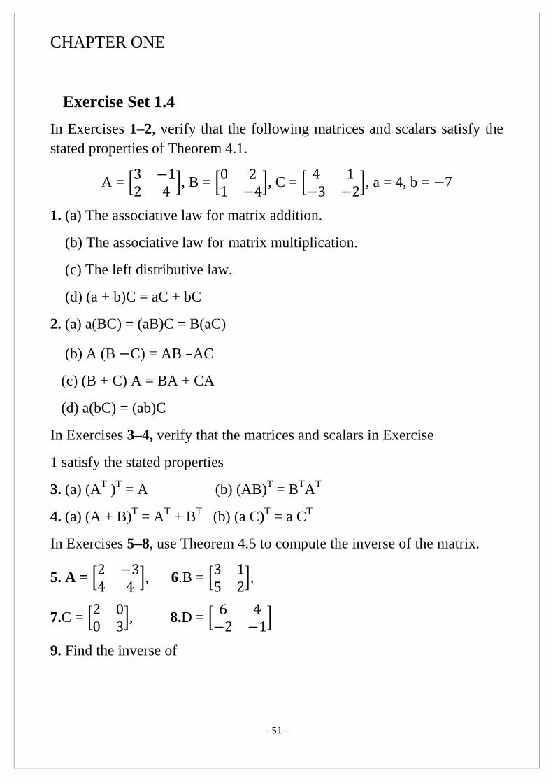
Exercise Set 1.4
In Exercises 1–2, verify that the following matrices and scalars satisfy the
stated properties of Theorem 4.1.
A = [3 −12 4
], B = [0 21 −4
], C = [4 1−3 −2
], a = 4, b = −7
1. (a) The associative law for matrix addition.
(b) The associative law for matrix multiplication.
(c) The left distributive law.
(d) (a + b)C = aC + bC
2. (a) a(BC) = (aB)C = B(aC)
(b) A (B −C) = AB –AC
(c) (B + C) A = BA + CA
(d) a(bC) = (ab)C
In Exercises 3–4, verify that the matrices and scalars in Exercise
1 satisfy the stated properties
3. (a) (AT )
T = A (b) (AB)
T = B
TA
T
4. (a) (A + B)T = A
T + B
T (b) (a C)
T = a C
T
In Exercises 5–8, use Theorem 4.5 to compute the inverse of the matrix.
5. A = [2 −34 4
], 6.B = [3 15 2
],
7.C = [2 00 3
], 8.D = [6 4−2 −1
]
9. Find the inverse of

CHAPTER ONE
- 52 -
[1/2(ex + e−x) 1/2(ex − e−x)
1/2(ex − e−x) 1/2(ex + e−x)].
10. Find the inverse of
[cos 𝜃 sin 𝜃− sin 𝜃 cos 𝜃
].
In Exercises 11–14, verify that the equations are valid for the matrices in
Exercises 5–8.
11. (AT )
-1 = (A
-1)T
12. (A-1
)-1
= A
13. (ABC)-1
= C-1
B-1
A-1
14. (ABC)T = C
TB
TA
T
In Exercises 15–18, use the given information to find A.
15. (7A)-1
= [−3 71 −2
] 16. (5AT )
-1 = [−3 −15 2
]
17. (I + 2A)-1
= [−1 24 5
] 18. A-1
= [2 −13 5
].
In Exercises 19–20, compute the following using the given matrix A.
(a) A3 (b) A
-3 (c) A
2 − 2A + I
19. A = [3 12 1
] 20. A = [2 04 1
].
In Exercises 21–22, compute p(A) for the given matrix A and the following
polynomials.
(a) p(x) = x − 2
(b) p(x) = 2x2 − x + 1
(c) p(x) = x3 − 2x + 1
21. A =[3 12 1
] 22. A = [2 04 1
].
In Exercises 23–24, let

CHAPTER ONE
- 53 -
A = [𝑎 𝑏𝑐 𝑑
] B = [0 10 0
] C = [0 01 0
]
23. Find all values of a, b, c, and d (if any) for which the matrices A and B
commute.
24. Find all values of a, b, c, and d (if any) for which the matrices A and C
commute.
In Exercises 25–28, use the method of Example 8 to find the unique
solution of the given linear system
25. 3x1 − 2x = −1
4x1 + 5x2 = 3
26. −x1 + 5x2 = 4
−x1 − 3x2 = 1
27. 6x1 + x2 = 0
4x1− 3x2 = −2
28. 2x1 − 2x2 = 4
x1 + 4x2 = 4.
If a polynomial p(x) can be factored as a product of lower degree
polynomials, say p(x) = p1(x)p2(x) and if A is a square matrix, then it can
be proved that p(A) = p1(A)p2(A).
In Exercises 29–30, verify this statement for the stated matrix A and
polynomials
p(x) = x2 − 9, p1(x) = x + 3, p2(x) = x − 3
29. The matrix A in Exercise 21.
30. An arbitrary square matrix A.
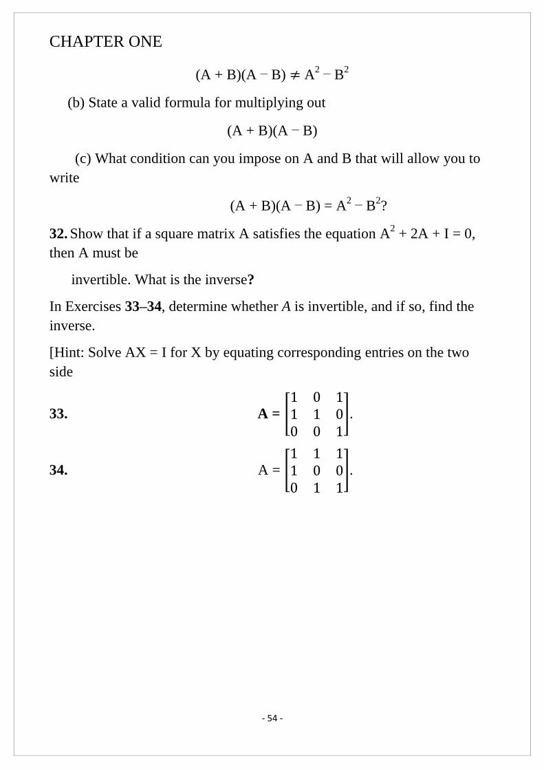
31. (a) Give an example of two 2 × 2 matrices such that
CHAPTER ONE
- 54 -
(A + B)(A − B) ≠ A2 − B
2
(b) State a valid formula for multiplying out
(A + B)(A − B)
(c) What condition can you impose on A and B that will allow you to
write
(A + B)(A − B) = A2 − B
2?
32. Show that if a square matrix A satisfies the equation A2 + 2A + I = 0,
then A must be
invertible. What is the inverse?
In Exercises 33–34, determine whether A is invertible, and if so, find the
inverse.
[Hint: Solve AX = I for X by equating corresponding entries on the two
side
33. A = [1 0 11 1 00 0 1
].
34. A = [1 1 11 0 00 1 1
].

CHAPTER ONE
- 55 -
1.5- Elementary Matrices and a Method for Finding A−1
In Section 1 we defined three elementary row operations on a matrix A:
1. Multiply a row by a nonzero constant c.
2. Interchange two rows.
3. Add a constant c times one row to another.
It should be evident that if we let B be the matrix that results from A by
performing one of the operations in this list, then the matrix A can be
recovered from B by performing the corresponding operation in the
following list:
1. Multiply the same row by 1/c.
2. Interchange the same two rows.
3. If B resulted by adding c times row ri of A to row rj , then add −c times rj
to ri .
It follows that if B is obtained from A by performing a sequence of
elementary row operations, then there is a second sequence of elementary
row operations, which when applied to B recovers A. Accordingly, we
make the following definition.
DEFINITION 1 Matrices A and B are said to be row equivalent if either
(hence each) can be obtained from the other by a sequence of elementary
row operations.
DEFINITION 2 A matrix E is called an elementary matrix if it can be
obtained from an identity matrix by performing a single elementary row
operation.

CHAPTER ONE
- 56 -
EXAMPLE 1 Elementary Matrices and Row Operations
Listed below are four elementary matrices and the operations that produce them.
[1 00 −3
], [1 0 30 1 00 0 1
] , [1 0 00 1 00 0 1
]
Multiply the second Add 3 times the third row of Multiply the first row
row of I2 by −3. I3 to the first row of I3 by 1
THEOREM 1.5.1 Row Operations by Matrix Multiplication
If the elementary matrix E results from performing a certain row operation
on Im and if A is an m × n matrix, then the product EA is the matrix that
results when this same row operation is performed on A.
EXAMPLE 2 Using Elementary Matrices
Consider the matrix
A = [1 0 2 32 −1 3 61 4 4 0
],
and consider the elementary matrix
E =[1 0 00 1 03 0 1
],
which results from adding 3 times the first row of I3 to the third row. The
product EA is
EA=[1 0 2 32 −1 3 64 4 10 9
],

CHAPTER ONE
- 57 -
which is precisely the matrix that results when we add 3 times the first row
of A to the third row.
We know from the discussion at the beginning of this section that if E is an
elementary matrix that results from performing an elementary row
operation on an identity matrix I, then there is a second elementary row
operation, which when applied to E produce I back again. Table 1 lists
these operations. The operations on the right side of the table are called the
inverse operations of the corresponding operations on the left.
Table 1
Row Operation on That Produces E Row Operation on E That
Reproduces I
Multiply row i by c ≠ 0 Multiply row i by 1/c
Interchange rows i and j Interchange rows i and j
Add c time row i to row j Add −c times row i to row j
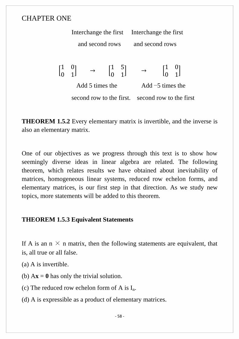
EXAMPLE 3 Row Operations and Inverse Row Operations
In each of the following, an elementary row operation is applied to the 2 ×
2 identity matrix to obtain an elementary matrix E, then E is restored to the
identity matrix by applying the inverse row operation.
[1 00 1
] → [1 00 7
] → [1 00 1
]
Multiply the second Multiply the second
row by 7. row by 1/7.
[1 00 1
] → [0 11 0
] → [1 00 1
]
CHAPTER ONE
- 58 -
Interchange the first Interchange the first
and second rows and second rows
[1 00 1
] → [1 50 1
] → [1 00 1
]
Add 5 times the Add −5 times the
second row to the first. second row to the first
THEOREM 1.5.2 Every elementary matrix is invertible, and the inverse is
also an elementary matrix.
One of our objectives as we progress through this text is to show how
seemingly diverse ideas in linear algebra are related. The following
theorem, which relates results we have obtained about inevitability of
matrices, homogeneous linear systems, reduced row echelon forms, and
elementary matrices, is our first step in that direction. As we study new
topics, more statements will be added to this theorem.
THEOREM 1.5.3 Equivalent Statements
If A is an n × n matrix, then the following statements are equivalent, that
is, all true or all false.
(a) A is invertible.
(b) Ax = 0 has only the trivial solution.
(c) The reduced row echelon form of A is In.
(d) A is expressible as a product of elementary matrices.

CHAPTER ONE
- 59 -
Inversion Algorithm To find the inverse of an invertible matrix A, find a
sequence of elementary row operations that reduces A to the identity and
then perform that same sequence of operations on In to obtain A-1
.
EXAMPLE 4 Using Row Operations to Find A-1
Find the inverse of
A = [1 2 32 5 31 0 8
].
To do this we will adjoin the identity matrix to the right side of A, thereby
producing a partitioned matrix of the form
[A | I]
Then we will apply row operations to this matrix until the left side is
reduced to I; these operations will convert the right side to A-1
, so the final
matrix will have the form
[I | A−1]
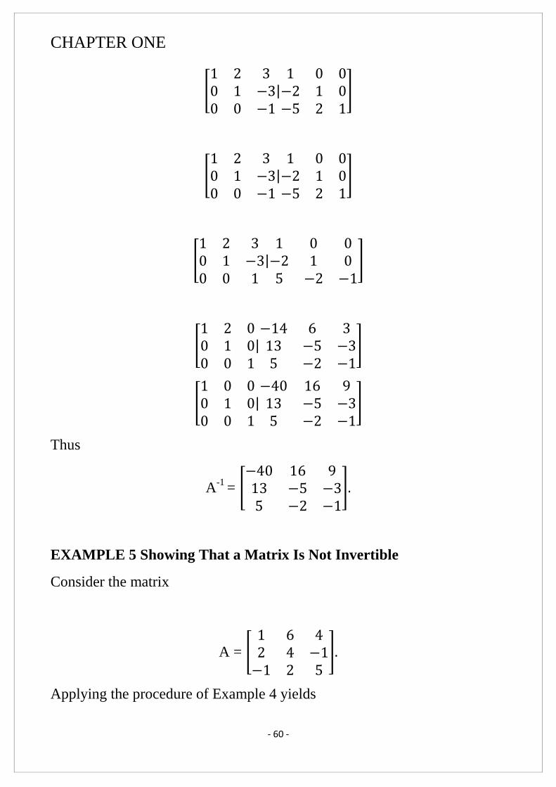
The computations are as follows:
[1 2 32 5 31 0 8
|1 0 00 1 00 0 1
]
[1 2 30 1 −30 −2 5
|1 0 0−2 1 0−1 0 1
]
CHAPTER ONE
- 60 -
[1 2 30 1 −30 0 −1
|1 0 0−2 1 0−5 2 1
]
[1 2 30 1 −30 0 −1
|1 0 0−2 1 0−5 2 1
]
[1 2 30 1 −30 0 1
|1 0 0−2 1 05 −2 −1
]
[1 2 00 1 00 0 1
|−14 6 313 −5 −35 −2 −1
]
[1 0 00 1 00 0 1
|−40 16 913 −5 −35 −2 −1
]
Thus
A-1
= [−40 16 913 −5 −35 −2 −1
].
EXAMPLE 5 Showing That a Matrix Is Not Invertible
Consider the matrix
A = [1 6 42 4 −1−1 2 5
].
Applying the procedure of Example 4 yields

CHAPTER ONE
- 61 -
[1 6 42 4 −1−1 2 5
|1 0 00 1 00 0 1
]
[1 6 40 −8 −90 8 9
|1 0 0−2 1 01 0 1
]
[1 6 40 −8 −90 0 0
|1 0 0−2 1 0−1 1 1
]
Since we have obtained a row of zeros on the left side, A is not invertible.
THEOREM 1.5.4
The matrix
A = [a bc d
]
is invertible if and only if ad − bc ≠ 0, in which case the inverse is given by
the formula−
𝐴−1 =1
𝑎𝑑 − 𝑏𝑐[𝑑 −𝑏−𝑐 𝑎
].
EXAMPLE 6 Analyzing Homogeneous Systems
a) x1 + 2 x2 + 3x3 = 0
2 x1 + 5 x2 + 3x3 = 0
x1 +8x3 = 0.

CHAPTER ONE
- 62 -
b) x1 + 6 x2 + 4x3 = 0
2x1 + 4 x2 − x3 = 0
− x1 + 2 x2 + 5x3 = 0.
From parts (a) and (b) of Theorem 5.3 a homogeneous linear system has
only the trivial solution if and only if its coefficient matrix is invertible.
From Examples 4 and 5 the coefficient matrix of system (a) is invertible
and that of system (b) is not. Thus, system (a) has only the trivial solution
while system (b) has nontrivial solutions.
CHAPTER ONE
- 63 -
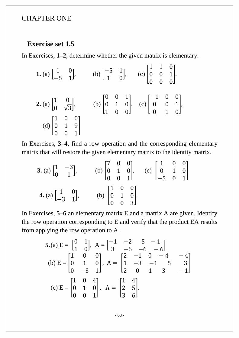
Exercise set 1.5
In Exercises, 1–2, determine whether the given matrix is elementary.
1. (a) [1 0−5 1
], (b) [−5 11 0
], (c) [1 1 00 0 10 0 0
].
2. (a) [1 0
0 √3], (b) [
0 0 10 1 01 0 0
], (c) [−1 0 00 0 10 1 0
],
(d) [1 0 00 1 90 0 1
]
In Exercises, 3–4, find a row operation and the corresponding elementary
matrix that will restore the given elementary matrix to the identity matrix.
3. (a) [1 −30 1
], (b) [7 0 00 1 00 0 1
], (c) [1 0 00 1 0−5 0 1
]
4. (a) [1 0−3 1
], (b) [1 0 00 1 00 0 3
].
In Exercises, 5–6 an elementary matrix E and a matrix A are given. Identify
the row operation corresponding to E and verify that the product EA results
from applying the row operation to A.
5. (a) E = [0 11 0
], A = [−1 −2 5 − 13 −6 −6 − 6
]
(b) E = [1 0 00 1 00 −3 1
] , A = [2 −1 0 − 4 − 41 −3 −1 5 32 0 1 3 − 1
]
(c) E = [1 0 40 1 00 0 1
] , A = [1 42 53 6
].

CHAPTER ONE
- 64 -
6. (a) E = [−6 00 1
], A = [−1 −2 5 − 13 −6 −6 − 6
]
(b) E = [1 0 0−4 1 00 0 1
] , 𝐴 = [2 −1 0 − 4 − 41 −3 −1 5 32 0 1 3 − 1
]
(c) E = [1 0 00 5 00 0 1
], 𝐴 = [1 42 53 6
].
In Exercises, 7–8, first use Theorem 5.4 and then use the inversion
algorithm to find A-1
, if it exists
7. (a) A = [1 42 7
] (b) A = [2 −4−4 8
].
8. (a) A = [1 −53 −16
] (b) A = [6 4−3 −2
].
In Exercises, 9–10, use the inversion algorithm to find the inverse of the
matrix (if the inverse exists).
9. (a) [1 2 32 5 31 0 8
] , (b) [−1 3 −42 4 1−4 2 −9
],
10. (a)
[ 1
5
1
5−2
51
5
1
5
1
101
5−4
5
1
10 ]
(b)
[ 1
5
1
5−2
52
5−3
5−
3
101
5−4
5
1
10 ]
.
In Exercises, 11–14, use the inversion algorithm to find the inverse of the
matrix (if the inverse exists).

CHAPTER ONE
- 65 -
11. [1 0 10 1 11 1 0
], 12. [√2 3√2 0
−4√2 √2 00 0 1
]
13. [2 6 62 7 62 7 7
] 14. [1 0 01 3 01 3 5
].
In Exercises, 15–16, find the inverse of each of the following 3 × 3
matrices, where k1, k2, k3, k4, and k are all nonzero.
15. (a) [
k1 0 0 0 k2 0 0 0 k3
], (b) [k 1 0 0 1 0 0 0 k
].
16. (a) [
0 0 k1 0 k2 0 k3 0 0
], (b) [k 0 0 1 k 0 0 1 k
].
In Exercises, 17–18, find all values of c, if any, for which the given matrix
is invertible.
17. [c c c 1 c c 1 1 c
] .
18. [c 1 0 1 c 1 0 1 c
].
CHAPTER ONE
- 66 -
1.6. More on Linear Systems and Invertible Matrices
THEOREM 1.6.1 A system of linear equations has zero, one, or infinitely
many solutions. There are no other possibilities.
THEOREM 1.6.2 If A is an invertible n × n matrix, then for each n × 1
matrix b, the system of equations Ax = b has exactly one solution, namely,
x = A-1
b.
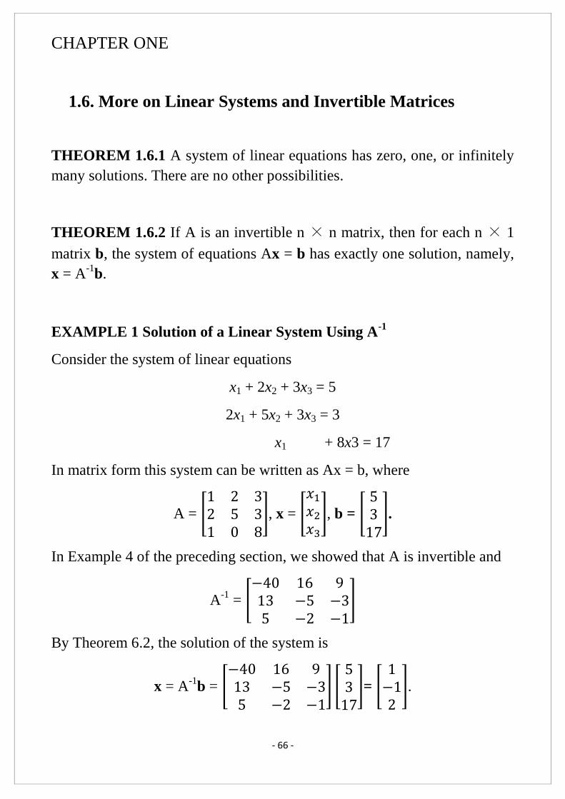
EXAMPLE 1 Solution of a Linear System Using A-1
Consider the system of linear equations
x1 + 2x2 + 3x3 = 5
2x1 + 5x2 + 3x3 = 3
x1 + 8x3 = 17
In matrix form this system can be written as Ax = b, where
A = [1 2 32 5 31 0 8
], x = [
𝑥1𝑥2𝑥3], b = [
5317].
In Example 4 of the preceding section, we showed that A is invertible and
A-1
= [−40 16 913 −5 −35 −2 −1
]
By Theorem 6.2, the solution of the system is
x = A-1
b = [−40 16 913 −5 −35 −2 −1
] [5317]= [
1−12].

CHAPTER ONE
- 67 -
or x1 = 1, x2 = −1, x3 = 2.
Frequently, one is concerned with solving a sequence of systems
Ax = b1, Ax = b2, Ax = b3, . . . , Ax = bk
each of which has the same square coefficient matrix A. If A is invertible,
then the solutions
x1 = A-1
b1, x2 = A-1
b2, x3 = A-1
b3, . . . , xk = A-1
bk
can be obtained with one matrix inversion and k matrix multiplications. An
efficient way to do this is to form the partitioned matrix
[⟨𝐴|𝑏1|𝑏𝑘⟩] (1)
in which the coefficient matrix A is “augmented” by all k of the matrices
b1, b2, . . . , bk, and then reduce (1) to reduced row echelon form by Gauss–
Jordan elimination. In this way we can solve all k systems at once. This
method has the added advantage that it applies even when A is not
invertible.
EXAMPLE 2 Solving Two Linear Systems at Once
Solve the systems
(a) x1 + 2x2 + 3x3 = 4
2x1 + 5x2 + 3x3 = 5
x1 + 8x3 = 9
(b) x1 + 2x2 + 3x3 = 1
2x1 + 5x2 + 3x3 = 6
x1 + 8x3 = −6
Solution The two systems have the same coefficient matrix. If we augment
this coefficient matrix with the columns of constants on the right sides of
these systems, we obtain
CHAPTER ONE
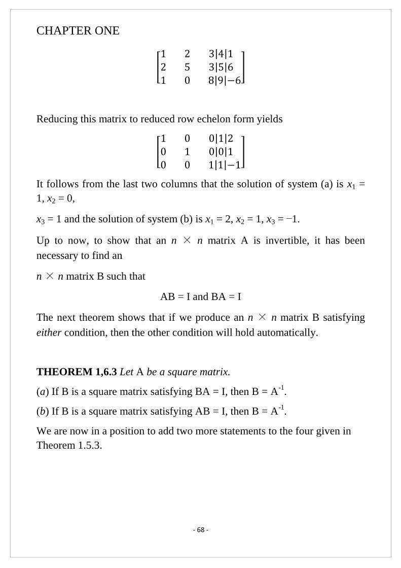
- 68 -
[1 2 3|4|12 5 3|5|61 0 8|9|−6
]
Reducing this matrix to reduced row echelon form yields
[1 0 0|1|20 1 0|0|10 0 1|1|−1
]
It follows from the last two columns that the solution of system (a) is x1 =
1, x2 = 0,
x3 = 1 and the solution of system (b) is x1 = 2, x2 = 1, x3 = −1.
Up to now, to show that an n × n matrix A is invertible, it has been
necessary to find an
n × n matrix B such that
AB = I and BA = I
The next theorem shows that if we produce an n × n matrix B satisfying
either condition, then the other condition will hold automatically.
THEOREM 1,6.3 Let A be a square matrix.
(a) If B is a square matrix satisfying BA = I, then B = A-1
.
(b) If B is a square matrix satisfying AB = I, then B = A-1
.
We are now in a position to add two more statements to the four given in
Theorem 1.5.3.
CHAPTER ONE
- 69 -
THEOREM 1.6.4 Equivalent Statements
If A is an n × n matrix, then the following are equivalent.
(a) A is invertible.
(b) Ax = 0 has only the trivial solution.
(c) The reduced row echelon form of A is In.
(d) A is expressible as a product of elementary matrices.
(e) Ax = b is consistent for every n × 1 matrix b.
( f ) Ax = b has exactly one solution for every n × 1 matrix b.
We know from earlier work that invertible matrix factors produce an
invertible product.
Conversely, the following theorem shows that if the product of square
matrices is invertible, then the factors themselves must be invertible.
THEOREM 1.6.5 Let A and B be square matrices of the same size. If AB
is invertible,
then A and B must also be invertible.
A Fundamental Problem Let A be a fixed m × n matrix. Find all m × 1
matrices b
such that the system of equations Ax = b is consistent.
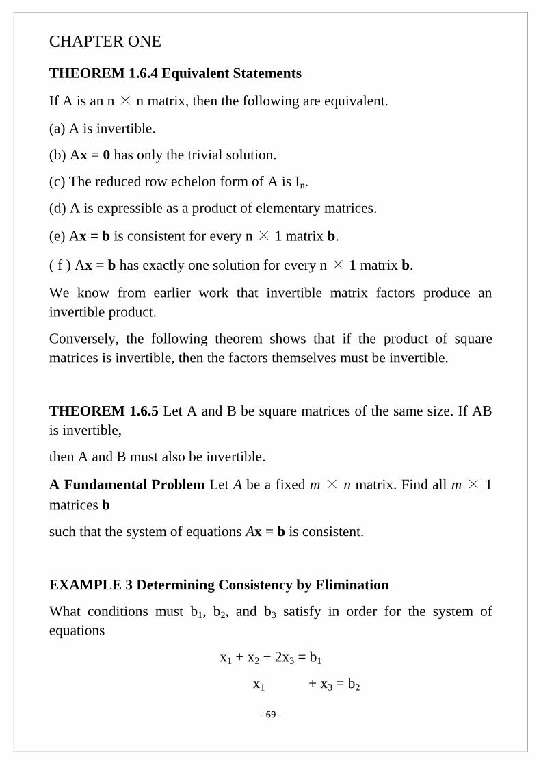
EXAMPLE 3 Determining Consistency by Elimination
What conditions must b1, b2, and b3 satisfy in order for the system of
equations
x1 + x2 + 2x3 = b1
x1 + x3 = b2
CHAPTER ONE
- 70 -
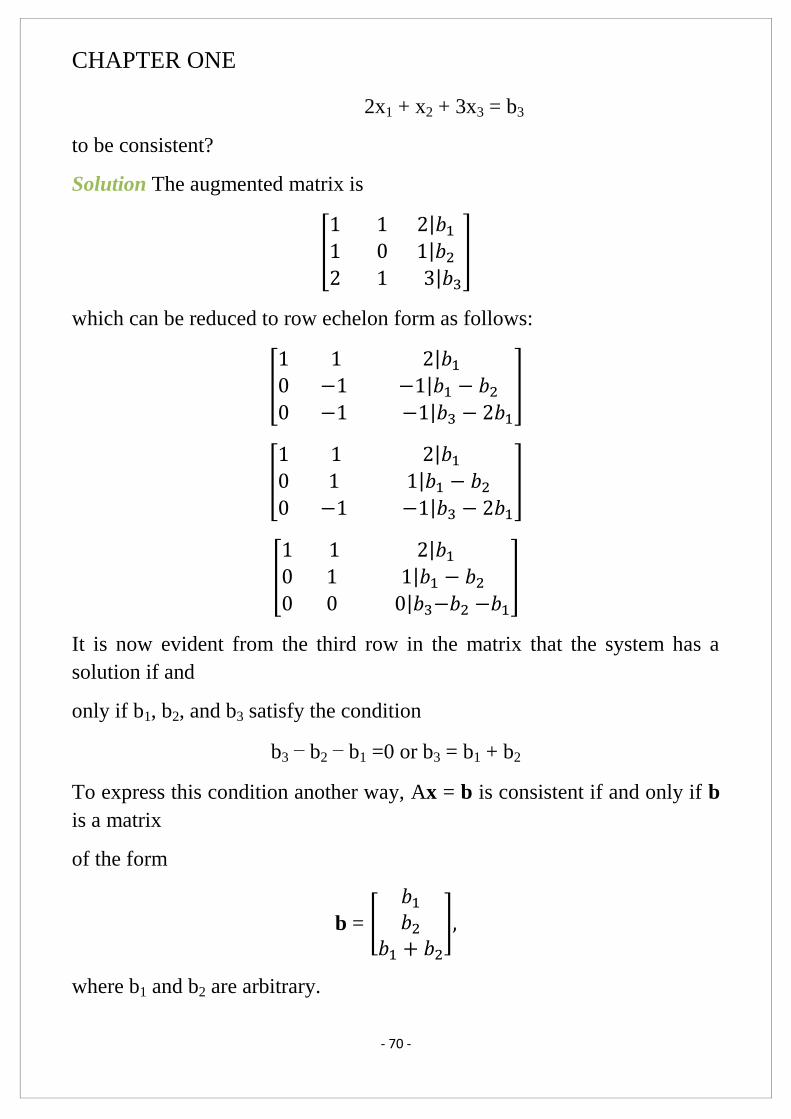
2x1 + x2 + 3x3 = b3
to be consistent?
Solution The augmented matrix is
[
1 1 2|𝑏11 0 1|𝑏22 1 3|𝑏3
]
which can be reduced to row echelon form as follows:
[
1 1 2|𝑏10 −1 −1|𝑏1 − 𝑏20 −1 −1|𝑏3 − 2𝑏1
]
[
1 1 2|𝑏10 1 1|𝑏1 − 𝑏20 −1 −1|𝑏3 − 2𝑏1
]
[
1 1 2|𝑏10 1 1|𝑏1 − 𝑏20 0 0|𝑏3−𝑏2 −𝑏1
]
It is now evident from the third row in the matrix that the system has a
solution if and
only if b1, b2, and b3 satisfy the condition
b3 − b2 − b1 =0 or b3 = b1 + b2
To express this condition another way, Ax = b is consistent if and only if b
is a matrix
of the form
b = [
𝑏1𝑏2
𝑏1 + 𝑏2
],
where b1 and b2 are arbitrary.
CHAPTER ONE
- 71 -
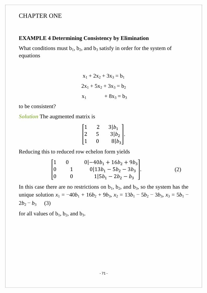
EXAMPLE 4 Determining Consistency by Elimination
What conditions must b1, b2, and b3 satisfy in order for the system of
equations
x1 + 2x2 + 3x3 = b1
2x1 + 5x2 + 3x3 = b2
x1 + 8x3 = b3
to be consistent?
Solution The augmented matrix is
[
1 2 3|𝑏12 5 3|𝑏21 0 8|𝑏3
].
Reducing this to reduced row echelon form yields
[
1 0 0|−40𝑏1 + 16𝑏2 + 9𝑏30 1 0|13𝑏1 − 5𝑏2 − 3𝑏30 0 1|5𝑏1 − 2𝑏2 − 𝑏3
]. (2)
In this case there are no restrictions on b1, b2, and b3, so the system has the
unique solution x1 = −40b1 + 16b2 + 9b3, x2 = 13b1 − 5b2 − 3b3, x3 = 5b1 −
2b2 − b3 (3)
for all values of b1, b2, and b3.

CHAPTER ONE
- 72 -
Exercise Set 1.6
In Exercises 1–7, solve the system by inverting the coefficient
matrix and using Theorem 1.6.2
1. x1 + x2 = 2
5x1 + 6x2 = 9.
2. 4x1 −3 x2 = −3
2x1 − 5x2 = 9.
3. x1 + 3x2 + x3 = 4
2x1 + 2x2 + x3 = −1
2x1 + 3x2 + x3 = 3.
4. x + y + z = 5
x + y − 4z = 10
−4x + y + z = 0.
5. x + y + z = 5
x + y − 4z = 10
−4x + y + z = 0.
6. 3x1 + 5x2 = b1
x1 + 2x2 = b2
7. x1 + 2x2 + 3x3 = b1
2x1 + 5x2 + 5x3 = b2
3x1 + 5x2 + 8x3 = b3

CHAPTER ONE
- 73 -
In Exercises 8–11, solve the linear systems together by reducing the
appropriate augmented matrix.
8. x1 − 5x2 = b1
3x1 + 2x2 = b2
(i) b1 = 1, b2 = 4 (ii) b1 = −2, b2 = 5.
9. −x1 + 4x2 + x3 = b1
x1 + 9x2 − 2x3 = b2
6x1 + 4x2 − 8x3 = b3
(i) b1 = 0, b2 = 1, b3 = 0
(ii) b1 = −3, b2 = 4, b3 = −5.
10. x1 + 3x2 + 5x3 = b1
−x1 − 2x2 = b2
2x1 + 5x2 + 4x3 = b3
(i) b1 = 1, b2 = 0, b3 = −1
(ii) b1 = 0, b2 = 1, b3 = 1
(iii) b1 = −1, b2 = −1, b3 = 0.
11. 4x1 − 7x2 = b1
x1 + 2x2 = b2
(i) b1 = 0, b2 = 1 (ii) b1 = −4, b2 = 6
(iii) b1 = −1, b2 =3 (iv)b1 = −5, b2 = 1.

CHAPTER ONE
- 74 -
In Exercises 12–15, determine conditions on the bi’s, if any, in order to
guarantee that the linear system is consistent.
12. x1 + 3x2 = b1
−2x1 + x2 = b2
13. 6x1 −4x2 = b1
3x1 −2 x2 = b2
14. x1 − 2x2 + 5x3 = b1
4x1 − 5x2 + 8x3 = b2
−3x1 + 3x2 − 3x3 = b3
15. x1 − x2 + 3x3 + 2x4 = b1
−2x1 + x2 + 5x3 + x4 = b2
−3x1 + 2x2 + 2x3 − x4 = b3
4x1 − 3x2 + x3 + 3x4 = b4
16.Consider the matrices
A = [2 1 22 2 −23 1 1
] and x = [
𝑥1x2𝑥3]
(a) Show that the equation Ax = x can be rewritten as (A − I)x = 0 and
use this result
to solve Ax = x for x.
(b) Solve Ax = 4x.

CHAPTER ONE
- 75 -
In Exercises 17–18, solve the matrix equation for X.
17. [1 −1 12 3 00 2 −1
] X = [2 −1 5 7 84 0 −3 0 13 5 −7 2 1
].
18. [−2 0 10 −1 −11 1 −4
] X = [4 3 2 16 7 8 91 3 7 9
].

CHAPTER ONE
- 76 -
1.7 Diagonal, Triangular, and Symmetric Matrices
A square matrix in which all the entries off the main diagonal are zero is
called a diagonal matrix. Here are some examples:
[2 00 −5
], [1 0 00 1 00 0 1
], [0 00 0
].
A general n × n diagonal matrix D can be written as
D = [
𝑑1 0 0 00 d2 0 00 0 d3 0
0 0 0 𝑑𝑛
]. (1)
A diagonal matrix is invertible if and only if all of its diagonal entries are
nonzero; in this case the inverse of (1) is
D-1
[
1/𝑑1 0 0 00 1/d2 0 00 0 1/d3 0 0 0 0 1/𝑑𝑛
]. (2)
Powers of diagonal matrices are easy to compute; we leave it for you to
verify that if D is the diagonal matrix (1) and k is a positive integer, then
Dk =
[ (𝑑1)
𝑘 0 0 0
0 (𝑑2)𝑘 0 0
0 0 (𝑑3)𝑘 0
0 0 0 (𝑑𝑛)𝑘]
. (3)
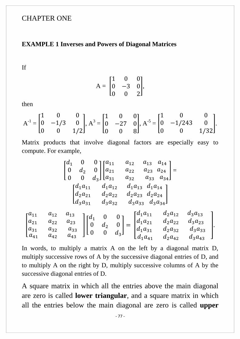
CHAPTER ONE
- 77 -
EXAMPLE 1 Inverses and Powers of Diagonal Matrices
If
A = [1 0 00 −3 00 0 2
],
then
A-1
= [
1 0 00 −1/3 00 0 1/2
], A3 = [1 0 00 −27 00 0 8
], A-5 = [
1 0 00 −1/243 00 0 1/32
].
Matrix products that involve diagonal factors are especially easy to
compute. For example,
[
𝑑1 0 00 𝑑2 00 0 𝑑3
] [
𝑎11 𝑎12 𝑎13 𝑎14𝑎21 𝑎22 𝑎23 𝑎24𝑎31 𝑎32 𝑎33 𝑎34
] =
[
𝑑1𝑎11 𝑑1𝑎12 𝑑1𝑎13 𝑑1𝑎14𝑑2𝑎21 𝑑2𝑎22 𝑑2𝑎23 𝑑2𝑎24𝑑3𝑎31 𝑑3𝑎32 𝑑3𝑎33 𝑑3𝑎34
]
[
𝑎11 𝑎12 𝑎13 𝑎21 𝑎22 𝑎23 𝑎31 𝑎32 𝑎33 𝑎41 𝑎42 𝑎43
] [
𝑑1 0 00 𝑑2 00 0 𝑑3
] = [
𝑑1𝑎11 𝑑2𝑎12 𝑑3𝑎13 𝑑1𝑎21 𝑑2𝑎22 𝑑3𝑎23 𝑑1𝑎31 𝑑2𝑎32 𝑑3𝑎33 𝑑1𝑎41 𝑑2𝑎42 𝑑3𝑎43
].
In words, to multiply a matrix A on the left by a diagonal matrix D,
multiply successive rows of A by the successive diagonal entries of D, and
to multiply A on the right by D, multiply successive columns of A by the
successive diagonal entries of D.
A square matrix in which all the entries above the main diagonal
are zero is called lower triangular, and a square matrix in which
all the entries below the main diagonal are zero is called upper

CHAPTER ONE
- 78 -
triangular. A matrix that is either upper triangular or lower
triangular is called triangular.
EXAMPLE 2 Upper and Lower Triangular Matrices
[
𝑎11 𝑎12 𝑎13 𝑎140 𝑎22 𝑎23 𝑎240 0 𝑎33 𝑎34 0 0 0 𝑎44
] general 4× 4 upper triangular matrix
[
𝑎11 0 0 0𝑎21 𝑎22 0 0𝑎31 𝑎32 𝑎33 0
𝑎41 𝑎42 𝑎43 𝑎44
] general 4× 4 lower triangular matrix
THEOREM 1.7.1
(a) The transpose of a lower triangular matrix is upper triangular, and the
transpose of an upper triangular matrix is lower triangular.
(b) The product of lower triangular matrices is lower triangular, and the
product of upper triangular matrices is upper triangular.
(c) A triangular matrix is invertible if and only if its diagonal entries are all
nonzero.
(d) The inverse of an invertible lower triangular matrix is lower triangular,
and the inverse of an invertible upper triangular matrix is upper triangular
EXAMPLE 3 Computations with Triangular Matrices
A = [1 3 −10 2 40 0 5
], B = [3 −2 20 0 −10 0 1
].
Then

CHAPTER ONE
- 79 -
A-1
= [
1 −3/2 7/50 1/2 −2/50 0 1/5
], AB = [3 −2 −20 0 20 0 5
], BA = [3 5 −10 0 −50 0 5
]
DEFINITION 1 A square matrix A is said to be symmetric if A = AT .
EXAMPLE 4 Symmetric Matrices
The following matrices are symmetric, since each is equal to its own
transpose.
[7 −3−3 5
] , [1 4 54 −3 05 0 7
], [
𝑑1 0 0 00 𝑑2 0 00 0 𝑑3 0
0 0 0 𝑑4
].
THEOREM 1.7.2 If A and B are symmetric matrices with the same size,
and if k is any scalar, then:
(a) AT is symmetric.
(b) A + B and A − B are symmetric.
(c) kA is symmetric
THEOREM 1.7.3 The product of two symmetric matrices is symmetric
if and only if the matrices commute.
EXAMPLE 5 Products of Symmetric Matrices
[1 22 3
] [−4 11 0
] = [−2 1−5 2
].
[1 22 3
] [4 33 −1
] = [2 11 3
].
The first matrix is not symmetric because the two matrices do not
commute.
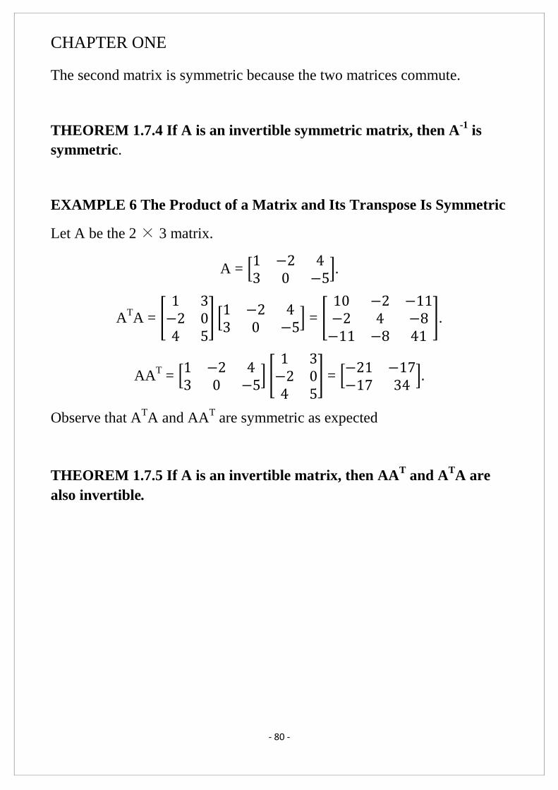
CHAPTER ONE
- 80 -
The second matrix is symmetric because the two matrices commute.
THEOREM 1.7.4 If A is an invertible symmetric matrix, then A-1
is
symmetric.
EXAMPLE 6 The Product of a Matrix and Its Transpose Is Symmetric
Let A be the 2 × 3 matrix.
A = [1 −2 43 0 −5
].
ATA = [
1 3−2 04 5
] [1 −2 43 0 −5
] = [10 −2 −11−2 4 −8−11 −8 41
].
AAT = [1 −2 43 0 −5
] [1 3−2 04 5
] = [−21 −17−17 34
].
Observe that ATA and AA
T are symmetric as expected
THEOREM 1.7.5 If A is an invertible matrix, then AAT and A
TA are
also invertible.

CHAPTER ONE
- 81 -
Exercise Set 1.7
In Exercises 1–2, classify the matrix as upper triangular, lower triangular,
or diagonal, and decide by inspection whether the matrix is invertible.
1. (a) [2 10 3
], (b) [0 04 0
], (c) [
−1 0 00 2 0
0 01
5
], (𝑑) [3 −2 70 0 30 0 8
].
2. (a) [4 01 7
], (b) [0 −30 0
] , (c) [4 0 00 3/5 00 0 −2
] , (𝑑) [3 0 03 1 07 0 0
].
In Exercises 3–6, find the product by inspection
𝟑. [3 0 03 −1 00 0 2
] [2 1−4 12 5
], 4. [1 2 −5−3 −1 0
] [−4 0 00 3 00 0 2
],
𝟓. [2 0 00 −1 00 0 4
] [4 −1 31 2 0−5 1 −2
] [2 0 00 −1 00 0 4
],
6. [5 0 00 2 00 0 −3
] [
1 2 0 41 5 3 06 2 2 2
].
In Exercises 7–9, find A2, A
-2, and A
-k (where k is any integer) by
inspection
7. A = [1 00 −2
], 8. A = [−6 0 00 3 00 0 5
], 9. A = [
1/2 0 00 1/3 00 0 1/4
].
In Exercises 10–11, compute the product by inspection
𝟏𝟎. [1 0 00 0 00 0 3
] [2 0 00 5 00 0 0
] [0 0 00 2 00 0 1
].

CHAPTER ONE
- 82 -
𝟏𝟏. [−1 0 00 2 00 0 4
] [3 0 00 5 00 0 7
] [5 0 00 −2 00 0 3
].
In Exercises 12–13, compute the indicated quantity.
12. [1 00 −1
]39
, 13. [1 00 −1
]1000
,
In Exercises 14–15, find all values of the unknown constant(s) for which
A is symmetric.
𝟏𝟒. [4 −3
a + 5 −1].
𝟏𝟓. [2 a − 2b + 2c 2a + b + c3 5 a + c0 −2 7
].
In Exercises 16–17, find all values of x for which A is invertible
16. A = [𝑥 − 1 𝑥2 𝑥4
0 𝑥 + 2 𝑥3
0 0 𝑥 − 4
].
17. A = [
𝑥 − 1/2 0 0𝑥 𝑥 − 1/3 0
x2 𝑥3 𝑥 + 1/4].
In Exercises 18–19, find a diagonal matrix A that satisfies the given
condition
18. A5 = [1 0 00 −1 00 0 −1
]. 19. A-2
=[9 0 00 4 00 0 1
].
20. Let A be an n × n symmetric matrix.
(a) Show that A2 is symmetric.
(b) Show that 2A2 − 3A + I is symmetric.
.

CHAPTER ONE
- 83 -
1.8 Matrix Transformations
Recall that in Section 1.1 we defined an “ordered n-tuple” to be a sequence
of n real numbers, and we observed that a solution of a linear system in n
unknowns, say
x1 = s1, x2 = s2, . . . , xn = sn can be expressed as the ordered n-tuple
(s1, s2, . . . , sn) (1)
Recall also that if n = 2, then the n-tuple is called an “ordered pair,” and if n
= 3, it is called an “ordered triple.” For two ordered n-tuples to be regarded
as the same, they must list the same numbers in the same order. Thus, for
example, (1, 2) and (2, 1) are different ordered pairs.
The set of all ordered n-tuples of real numbers is denoted by the symbol Rn.
The elements of Rn are called vectors and are denoted in boldface type,
such as a, b, v, w, and x. When convenient, ordered n-tuples can be denoted
in matrix notation as column vectors. For example, the matrix
[
s1s2...sn
] (2)
can be used as an alternative to (1). We call (1) the comma-delimited form
of a vector and (2) the column-vector form. For each i = 1, 2, . . . , n, let ei
denote the vector in Rn
with a 1 in the ith
position and zeros elsewhere. In
column form these vectors are
e1 = [ 100] , 𝑒2 = [
010], … en = [
001].
We call the vectors e1, e2, . . . , en the standard basis vectors for Rn. For
example, the vectors
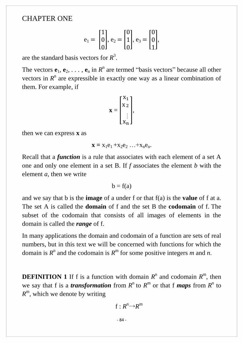
CHAPTER ONE
- 84 -
e1 = [100], e2 = [
010], e3 = [
001],
are the standard basis vectors for R3.
The vectors e1, e2, . . . , en in Rn are termed “basis vectors” because all other
vectors in Rn are expressible in exactly one way as a linear combination of
them. For example, if
x = [
x1x 2...xn
],
then we can express x as
x = x1e1 +x2e2 …+xnen.
Recall that a function is a rule that associates with each element of a set A
one and only one element in a set B. If f associates the element b with the
element a, then we write
b = f(a)
and we say that b is the image of a under f or that f(a) is the value of f at a.
The set A is called the domain of f and the set B the codomain of f. The
subset of the codomain that consists of all images of elements in the
domain is called the range of f.
In many applications the domain and codomain of a function are sets of real
numbers, but in this text we will be concerned with functions for which the
domain is Rn and the codomain is R
m for some positive integers m and n.
DEFINITION 1 If f is a function with domain Rn and codomain R
m, then
we say that f is a transformation from Rn
to Rm
or that f maps from Rn to
Rm
, which we denote by writing
f : Rn→R
m

CHAPTER ONE
- 85 -
In the special case where m = n, a transformation is sometimes called an
operator on Rn.
In this section we will be concerned with the class of transformations from
Rn to R
m that arise from linear systems. Specifically, suppose that we have
the system of linear equations
w1 = a11x1 + a12x2 + · · · + a1nxn
w2 = a21x1 + a22x2 + · · · + a2nxn
. . . .
. . . .
(3)
. . . .
wm = am1x1 + am2x2 + · · · + amnxn
which we can write in matrix notation as
[
w1w2...
wm
] = [
𝑎11 𝑎12 𝑎1𝑛𝑎21 𝑎22 𝑎2𝑛
𝑎𝑚1 𝑎𝑚2 𝑎𝑚𝑛
] [
x1x 2...xn
], (4)
or more briefly as
w = A x. (5)
Although we could view (5) as a compact way of writing linear system (3),
we will view it instead as a transformation that maps a vector x in Rn into
the vector w in Rm
by multiplying x on the left by A. We call this a matrix
transformation (or matrix operator in the special case where m = n). We
denote it by
TA: Rn → R
m

CHAPTER ONE
- 86 -
This notation is useful when it is important to make the domain and
codomain clear. The subscript on TA serves as a reminder that the
transformation results from multiplying vectors in Rn by the matrix A. In
situations where specifying the domain and codomain is not essential, we
will express (4) as
w = TA(x) (6)
We call the transformation TA multiplication by A. On occasion we will
find it convenient to express (6) in the schematic form
𝐱 𝑇𝐴→ 𝐰, (7)
which is read “TA maps x into w.”
EXAMPLE 1 A Matrix Transformation from R4 to R
3
The transformation from R4 to R
3 defined by the equations
w1 = 2x1 − 3x2 + x3 − 5x4
w2 = 4x1 + x2 − 2x3 + x4 (8)
w3 = 5x1 − x2 + 4x3,
can be expressed in matrix form as
[
w1w2w3] = [
2 −3 1 − 54 1 −2 15 −1 4 0
] [
𝑥1𝑥2𝑥3𝑥4
],
from which we see that the transformation can be interpreted as
multiplication by
A = [2 −3 1 − 54 1 −2 15 −1 4 0
]. (9)
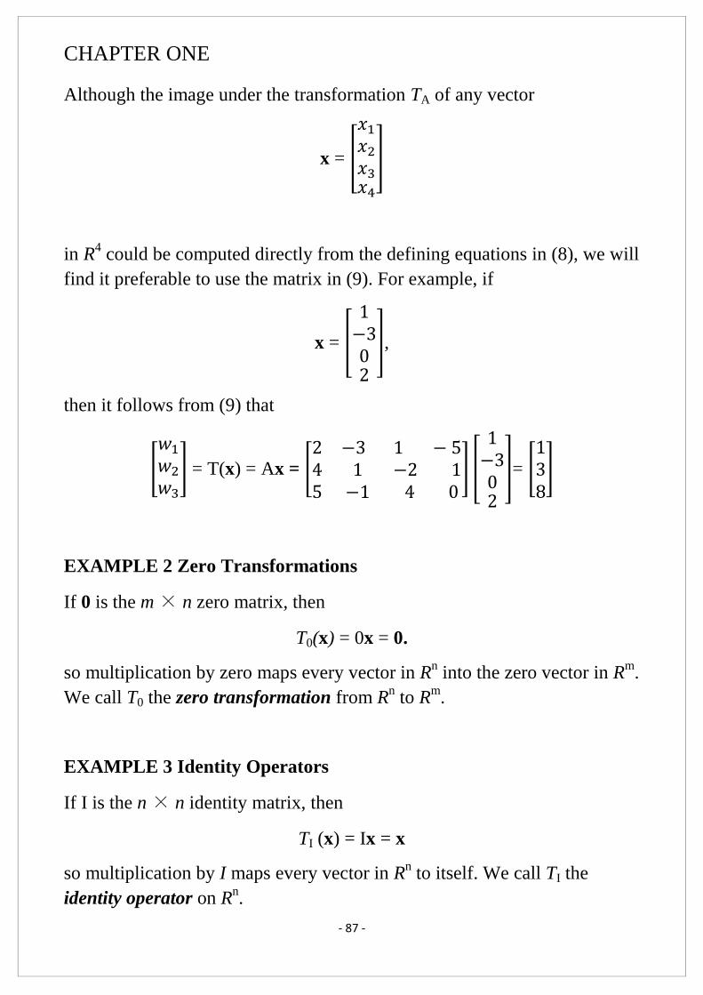
CHAPTER ONE
- 87 -
Although the image under the transformation TA of any vector
x = [
𝑥1𝑥2𝑥3𝑥4
]
in R4 could be computed directly from the defining equations in (8), we will
find it preferable to use the matrix in (9). For example, if
x = [
1−302
],
then it follows from (9) that
[
𝑤1𝑤2𝑤3] = T(x) = Ax = [
2 −3 1 − 54 1 −2 15 −1 4 0
] [
1−302
]= [138]
EXAMPLE 2 Zero Transformations
If 0 is the m × n zero matrix, then
T0(x) = 0x = 0.
so multiplication by zero maps every vector in Rn into the zero vector in R
m.
We call T0 the zero transformation from Rn to R
m.
EXAMPLE 3 Identity Operators
If I is the n × n identity matrix, then
TI (x) = Ix = x
so multiplication by I maps every vector in Rn to itself. We call TI the
identity operator on Rn.
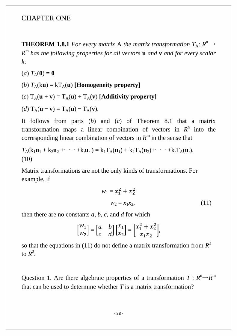
CHAPTER ONE
- 88 -
THEOREM 1.8.1 For every matrix A the matrix transformation TA: Rn →
Rm
has the following properties for all vectors u and v and for every scalar
k:
(a) TA(0) = 0
(b) TA(ku) = kTA(u) [Homogeneity property]
(c) TA(u + v) = TA(u) + TA(v) [Additivity property]
(d) TA(u − v) = TA(u) − TA(v).
It follows from parts (b) and (c) of Theorem 8.1 that a matrix
transformation maps a linear combination of vectors in Rn into the
corresponding linear combination of vectors in Rm
in the sense that
TA(k1u1 + k2u2 +· · ·+krur ) = k1TA(u1) + k2TA(u2)+· · ·+krTA(ur).
(10)
Matrix transformations are not the only kinds of transformations. For
example, if
w1 = 𝑥12 + 𝑥2
2
w2 = x1x2, (11)
then there are no constants a, b, c, and d for which
[𝑤1𝑤2] = [
𝑎 𝑏𝑐 𝑑
] [𝑥1𝑥2] = [
𝑥12 + 𝑥2
2
𝑥1𝑥2],
so that the equations in (11) do not define a matrix transformation from R2
to R2.
Question 1. Are there algebraic properties of a transformation T : Rn→R
m
that can be used to determine whether T is a matrix transformation?
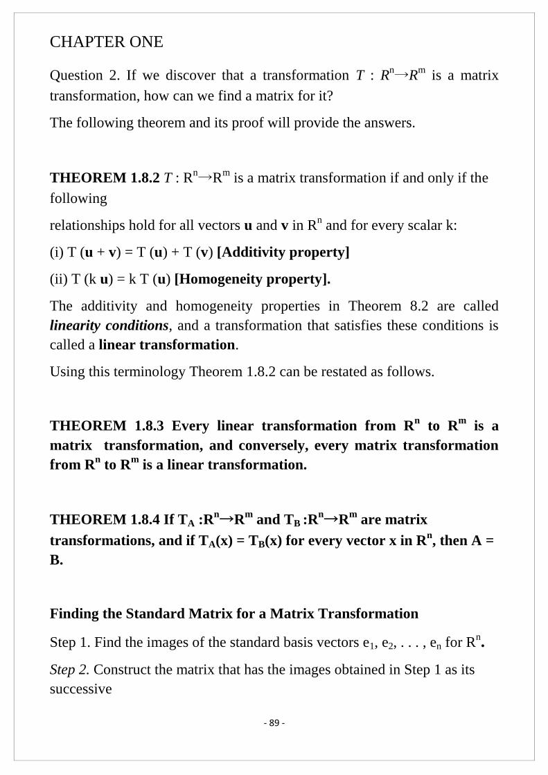
CHAPTER ONE
- 89 -
Question 2. If we discover that a transformation T : Rn→R
m is a matrix
transformation, how can we find a matrix for it?
The following theorem and its proof will provide the answers.
THEOREM 1.8.2 T : Rn→R
m is a matrix transformation if and only if the
following
relationships hold for all vectors u and v in Rn and for every scalar k:
(i) T (u + v) = T (u) + T (v) [Additivity property]
(ii) T (k u) = k T (u) [Homogeneity property].
The additivity and homogeneity properties in Theorem 8.2 are called
linearity conditions, and a transformation that satisfies these conditions is
called a linear transformation.
Using this terminology Theorem 1.8.2 can be restated as follows.
THEOREM 1.8.3 Every linear transformation from Rn to R
m is a
matrix transformation, and conversely, every matrix transformation
from Rn to R
m is a linear transformation.
THEOREM 1.8.4 If TA :Rn→R
m and TB :R
n→Rm
are matrix
transformations, and if TA(x) = TB(x) for every vector x in Rn, then A =
B.
Finding the Standard Matrix for a Matrix Transformation
Step 1. Find the images of the standard basis vectors e1, e2, . . . , en for Rn.
Step 2. Construct the matrix that has the images obtained in Step 1 as its
successive
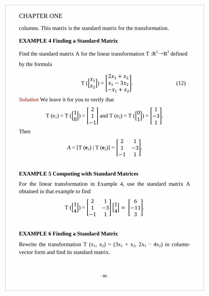
CHAPTER ONE
- 90 -
columns. This matrix is the standard matrix for the transformation.
EXAMPLE 4 Finding a Standard Matrix
Find the standard matrix A for the linear transformation T :R2→R
2 defined
by the formula
T ([𝑥1𝑥2]) = [
2𝑥1 + 𝑥2𝑥1 − 3𝑥2−𝑥1 + 𝑥2
]. (12)
Solution We leave it for you to verify that
T (e1) = T ([10]) = [
21−1] and T (e2) = T ([
01]) = [
1−31].
Then
A = [T (e1) | T (e2)] = [2 11 −3−1 1
].
EXAMPLE 5 Computing with Standard Matrices
For the linear transformation in Example 4, use the standard matrix A
obtained in that example to find
T ([14]) = [
2 11 −3−1 1
] [14] = [
6−113].
EXAMPLE 6 Finding a Standard Matrix
Rewrite the transformation T (x1, x2) = (3x1 + x2, 2x1 − 4x2) in column-
vector form and find its standard matrix.

CHAPTER ONE
- 91 -
Solution
T ([𝑥1𝑥2]) = [
3𝑥1 + 𝑥22𝑥1 − 4𝑥2
] = [3 12 −4
] [x1x2].
Thus, the standard matrix is
[3 12 −4
].

CHAPTER ONE
- 92 -
Exercise Set 1.8
In Exercises 1–2, find the domain and codomain of the transformation
TA(x) = Ax.
1. (a) A has size 3 × 2. (b) A has size 2 × 3.
(c) A has size 3 × 3. (d) A has size 1 × 6.
2. (a) A has size 4 × 5. (b) A has size 5 × 4.
(c) A has size 4 × 4. (d) A has size 3 × 1.
In Exercises 3–4, find the domain and codomain of the transformation
defined by the equations
3. (a) w1 = 4x1 + 5x2
w2 = x1 − 8x2
(b) w1 = 5x1 − 7x2
w2 = 6x1 + x2
w3 = 2x1 + 3x2.
4. (a) w1 = x1 − 4x2 + 8x3
w2 = −x1 + 4x2 + 2x3
w3 = −3x1 + 2x2 − 5x3
(b) w1 = 2x1 + 7x2 − 4x3
w2 = 4x1 − 3x2 + 2x3.
In Exercises 5–6, find the standard matrix for the transformation defined
by the equations
5. (a) [3 1 26 7 1
] [
𝑥1𝑥2𝑥3] (b) [
2 −14 32 −5
] [x1x2].
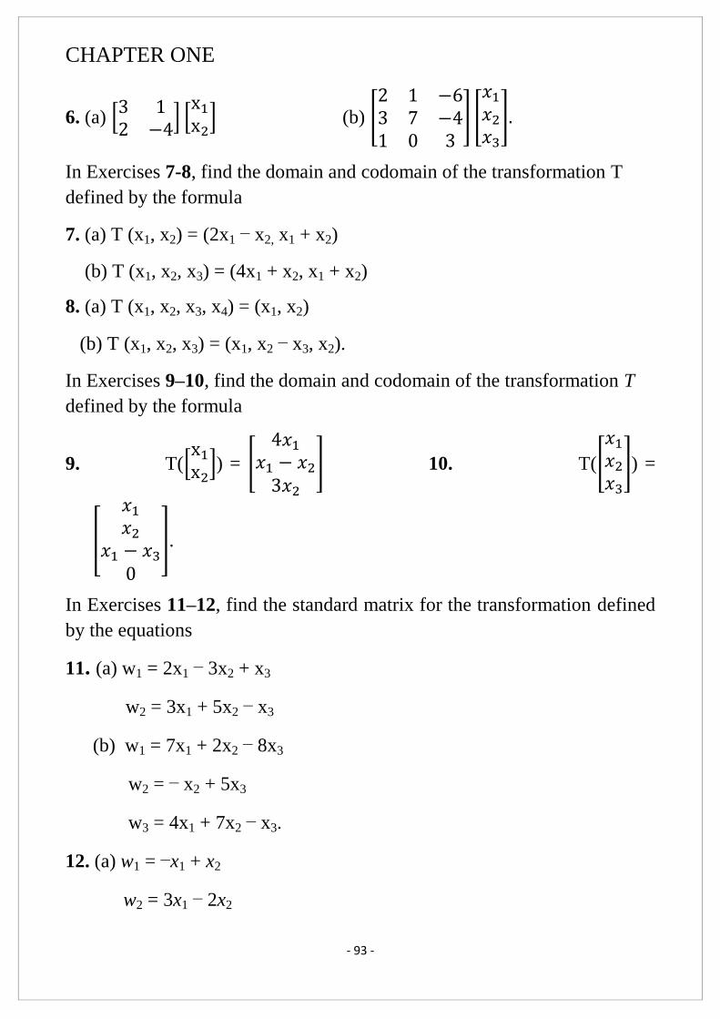
CHAPTER ONE
- 93 -
6. (a) [3 12 −4
] [x1x2] (b) [
2 1 −63 7 −41 0 3
] [
𝑥1𝑥2𝑥3].
In Exercises 7-8, find the domain and codomain of the transformation T
defined by the formula
7. (a) T (x1, x2) = (2x1 − x2, x1 + x2)
(b) T (x1, x2, x3) = (4x1 + x2, x1 + x2)
8. (a) T (x1, x2, x3, x4) = (x1, x2)
(b) T (x1, x2, x3) = (x1, x2 − x3, x2).
In Exercises 9–10, find the domain and codomain of the transformation T
defined by the formula
9. T([x1x2]) = [
4𝑥1𝑥1 − 𝑥23𝑥2
] 10. T([
𝑥1𝑥2𝑥3]) =
[
𝑥1𝑥2
𝑥1 − 𝑥30
].
In Exercises 11–12, find the standard matrix for the transformation defined
by the equations
11. (a) w1 = 2x1 − 3x2 + x3
w2 = 3x1 + 5x2 − x3
(b) w1 = 7x1 + 2x2 − 8x3
w2 = − x2 + 5x3
w3 = 4x1 + 7x2 − x3.
12. (a) w1 = −x1 + x2
w2 = 3x1 − 2x2
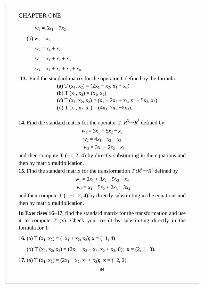
CHAPTER ONE
- 94 -
w3 = 5x1 − 7x2
(b) w1 = x1
w2 = x1 + x2
w3 = x1 + x2 + x3
w4 = x1 + x2 + x3 + x4.
13. Find the standard matrix for the operator T defined by the formula.
(a) T (x1, x2) = (2x1 − x2, x1 + x2)
(b) T (x1, x2) = (x1, x2)
(c) T (x1, x2, x3) = (x1 + 2x2 + x3, x1 + 5x2, x3)
(d) T (x1, x2, x3) = (4x1, 7x2,−8x3).
14. Find the standard matrix for the operator T :R3→R
3 defined by:
w1 = 3x1 + 5x2 − x3
w2 = 4x1 − x2 + x3
w3 = 3x1 + 2x2 − x3
and then compute T (−1, 2, 4) by directly substituting in the equations and
then by matrix multiplication.
15. Find the standard matrix for the transformation T :R4→R
2 defined by
w1 = 2x1 + 3x2 − 5x3 − x4
w2 = x1 − 5x2 + 2x3 − 3x4
and then compute T (1,−1, 2, 4) by directly substituting in the equations and
then by matrix multiplication.
In Exercises 16–17, find the standard matrix for the transformation and use
it to compute T (x). Check your result by substituting directly in the
formula for T.
16. (a) T (x1, x2) = (−x1 + x2, x2); x = (−1, 4)
(b) T (x1, x2, x3) = (2x1 − x2 + x3, x2 + x3, 0); x = (2, 1,−3).
17. (a) T (x1, x2) = (2x1 − x2, x1 + x2); x = (−2, 2)

CHAPTER ONE
- 95 -
(b) T (x1, x2, x3) = (x1, x2 − x3, x2); x = (1, 0, 5).
In Exercises 18–19, find TA(x), and express your answer in matrix form.
18. (a) A = [1 23 4
], x = [3−2]
(b) A = [−1 2 03 1 5
], x = [−113].
19. (a) A = [−2 1 43 5 76 0 −1
], x =[
x1x2x3]
(b)A = [−1 12 47 8
], x = [x1x2].

CHAPTER TWO
- 96 -
C H A P T E R TWO
Determinants

CHAPTER TWO
- 97 -
2.1 Determinants by Cofactor Expansion
Recall from Theorem 4.5 that the 2 × 2 matrix
A = [𝑎 𝑏𝑐 𝑑
],
is invertible if and only if ad−bc≠ 0, and the expansion ad−bc is called
the determinant of the matrix A. Recall also that this determinant is
denoted by writing
det (A) = ad−bc or |𝑎 𝑏𝑐 𝑑
| = ad−bc, (1)
and that the inverse of A can be expressed in terms of the determinant as
A-1
= 1
det (A) [𝑑 −𝑏−𝑐 𝑎
]. (2)
Thus, if we denote a 2 × 2 matrix as
A = [𝑎11 𝑎12𝑎21 𝑎22
],
then the two equations in (1) take the form
det (A) = |a11 a12a21 a22
| = 𝑎11𝑎22 − 𝑎12𝑎21. (3)
In situations where it is inconvenient to assign a name to the matrix, we
can express this formula as
det [𝑎11 𝑎12𝑎21 𝑎22
] = 𝑎11𝑎22 − 𝑎12𝑎21. (4)
To start the process, let us define the determinant of a 1 × 1 matrix [a11]
as
det [a11] = a11, (5)
from which it follows that Formula (4) can be expressed as

CHAPTER TWO
- 98 -
det [𝑎11 𝑎12𝑎21 𝑎22
] = det [𝑎11] det [𝑎22] − det [𝑎12]det [𝑎21].
DEFINITION 1 If A is a square matrix, then the minor of entry aij is
denoted by Mij and is defined to be the determinant of the submatrix that
remains after the ith row and jth column are deleted from A. The number (−
1)i+j
Mij is denoted by Cij and is called the cofactor of entry aij.
EXAMPLE 1 Finding Minors and Cofactors
Let
A = [3 1 −42 5 61 4 8
].
The minor of entry a11 is
M11 = [5 64 8
] = 16.
The cofactor of a11 is
C11 = (−1)1+1
M11 = M11 = 16.
Similarly, the minor of entry a32 is
M32 = [3 −42 6
] = 26.
The cofactor of a32 is
C32 = (−1)3+2
M32 = − M32 = −26.

CHAPTER TWO
- 99 -
EXAMPLE 2 Cofactor Expansions of a 2 × 2 Matrix
The checkerboard pattern for a 2 × 2 matrix A = [aij] is
[+ −− +
],
so that
C11 = M11 = a22 C12 = −M12 = −a21
C21 = −M21 = −a12 C22 = M22 = a11.
we leave it for you to use Formula (3) to verify that det(A) can be
expressed in terms of cofactors in the following four ways:
det(A) = |𝑎11 𝑎12𝑎21 𝑎22
|
= a11C11 + a12C12
= a21C21 + a22C22 (6)
= a11C11 + a21C21
= a12C12 + a22C22.
Each of the last four equations is called a cofactor expansion of det(A). In
each cofactor expansion the entries and cofactors all come from the same
row or same column of A. For example, in the first equation the entries and
cofactors all come from the first row of A, in the second they all come
from the second row of A, in the third they all come from the first column
of A, and in the fourth they all come from the second column of A.
THEOREM 2.1.1 If A is an n × n matrix, then regardless of which row
or column of A is chosen, the number obtained by multiplying the entries
in that row or column by the corresponding cofactors and adding the
resulting products is always the same.

CHAPTER TWO
- 100 -
DEFINITION 2 If A is an n × n matrix, then the number obtained by
multiplying the entries in any row or column of A by the corresponding
cofactors and adding the resulting products is called the determinant of A,
and the sums themselves are called cofactor expansions of A. That is,
det(A) = a1jC1j + a2jC2j +· · ·+anjCnj (7)
[cofactor expansion along the jth column]
and
det(A) = ai1Ci1 + ai2Ci2 +· · ·+ainCin (8)
[cofactor expansion along the ith row]
EXAMPLE 3 Cofactor Expansion Along the First Row
Find the determinant of the matrix
A = [3 1 0−2 −4 35 4 −2
],
by cofactor expansion along the first row.
Solution
det(A) = |3 1 0−2 −4 35 4 −2
| = 3|−4 34 −2
| − |−2 35 −2
| +0 |−2 −45 4
|
= 3(−4) −1(−11) +0 = −1.
EXAMPLE 4 Cofactor Expansion Along the First Column
Let A be the matrix in Example 3, and evaluate det(A) by cofactor
expansion along the first column of A.

CHAPTER TWO
- 101 -
Solution
det(A) = |3 1 0−2 −4 35 4 −2
| = 3|−4 34 −2
| −(−2) |1 04 −2
| + 5 |1 0−4 3
|
= 3(−4) − (−2)(−2) + 5(3) = −1
This agrees with the result obtained in Example 3.
EXAMPLE 5 Smart Choice of Row or Column
If A is the 4 × 4 matrix
A = [
1 0 0 − 13 1 2 21 0 −2 12 0 0 1
],
then to find det(A) it will be easiest to use cofactor expansion along the
second column, since it has the most zeros:
det (A) = 1|1 0 −11 −2 12 0 1
|.
For the 3 × 3 determinant, it will be easiest to use cofactor expansion
along its second column, since it has the most zeros:
det (A) = 1. −2 . |1 −12 1
|
= (−2)(1+2)
= −6.

CHAPTER TWO
- 102 -
EXAMPLE 6 Determinant of a Lower Triangular Matrix
The following computation shows that the determinant of a 4 × 4 lower
triangular matrix is the product of its diagonal entries. Each part of the
computation uses a cofactor expansion along the first row.
|
𝑎11 0 0 0𝑎21 𝑎22 0 0𝑎31 𝑎32 𝑎33 0𝑎41 𝑎42 𝑎43 𝑎44
| = 𝑎11𝑎22 |𝑎33 0𝑎43 a44
|
= 𝑎11𝑎22 𝑎33|𝑎44|
= 𝑎11𝑎22 𝑎33a44.
THEOREM 2.1.2 If A is an n × n triangular matrix (upper triangular,
lower triangular, or diagonal), then det(A) is the product of the entries on
the main diagonal of the matrix; that is, det(A) = a11a22 · · · ann.
Determinants of 2 × 2 and 3 × 3 matrices can be evaluated very
efficiently using the pattern suggested in Figure 2.1
[𝑎11 𝑎12𝑎21 𝑎22
] [
𝑎11 𝑎12 𝑎13𝑎21 𝑎22 𝑎23𝑎31 𝑎32 𝑎33
]
𝑎11 𝑎12𝑎22 𝑎22𝑎31 𝑎32
Figure 8.2.1
In the 2 × 2 case, the determinant can be computed by forming the
product of the entries on the rightward arrow and subtracting the product
of the entries on the leftward arrow. In the 3 × 3 case we first recopy the
first and second columns as shown in the figure, after which we can
compute the determinant by summing the products of the entries on the
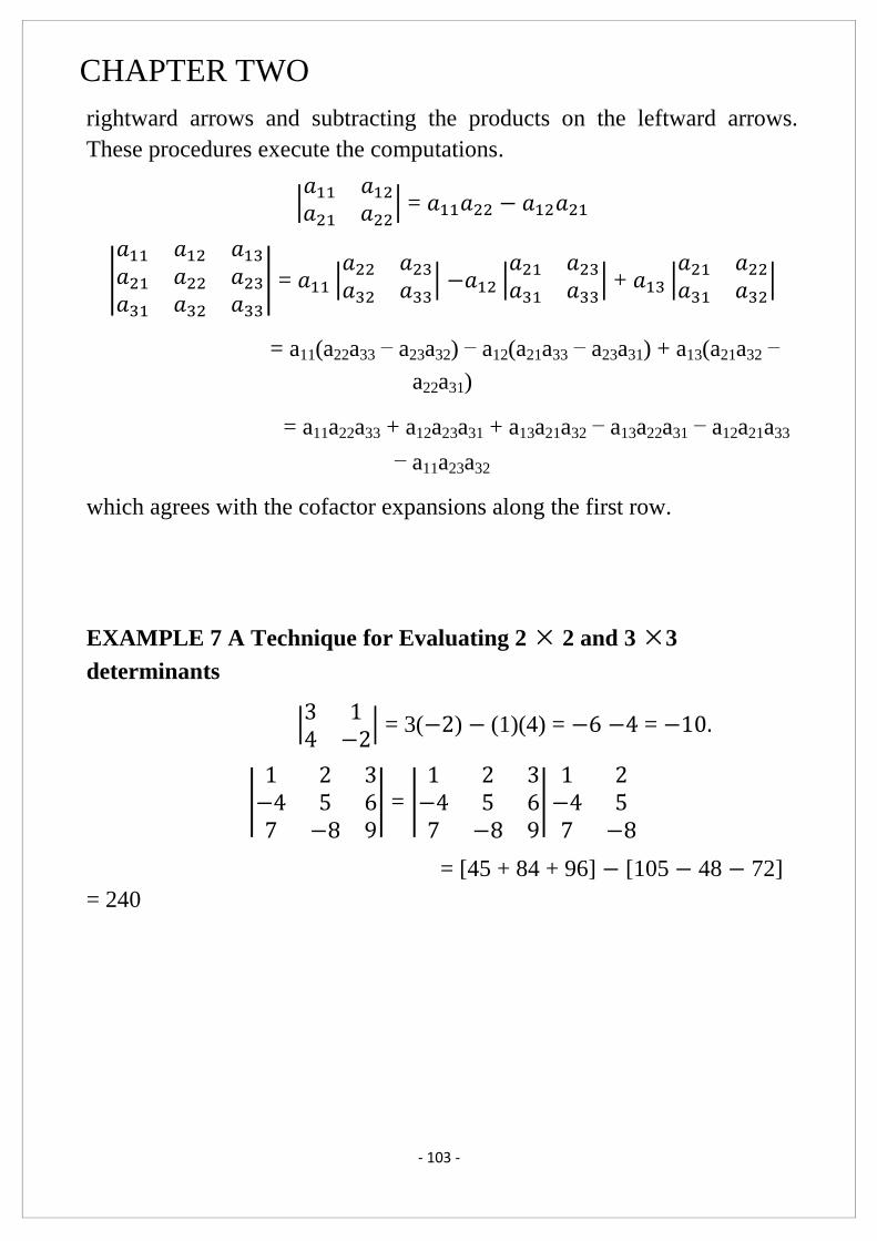
CHAPTER TWO
- 103 -
rightward arrows and subtracting the products on the leftward arrows.
These procedures execute the computations.
|𝑎11 𝑎12𝑎21 𝑎22
| = 𝑎11𝑎22 − 𝑎12𝑎21
|
𝑎11 𝑎12 𝑎13𝑎21 𝑎22 𝑎23𝑎31 𝑎32 𝑎33
| = 𝑎11 |𝑎22 𝑎23𝑎32 𝑎33
| −𝑎12 |𝑎21 𝑎23𝑎31 𝑎33
| + 𝑎13 |𝑎21 𝑎22𝑎31 𝑎32
|
= a11(a22a33 − a23a32) − a12(a21a33 − a23a31) + a13(a21a32 −
a22a31)
= a11a22a33 + a12a23a31 + a13a21a32 − a13a22a31 − a12a21a33
− a11a23a32
which agrees with the cofactor expansions along the first row.
EXAMPLE 7 A Technique for Evaluating 2 × 2 and 3 ×3
determinants
|3 14 −2
| = 3(−2) − (1)(4) = −6 −4 = −10.
|1 2 3−4 5 67 −8 9
| = |1 2 3−4 5 67 −8 9
|1 2−4 57 −8
= [45 + 84 + 96] − [105 − 48 − 72]
= 240

CHAPTER TWO
- 104 -
Exercise Set 2.1
In Exercises 1–2, find all the minors and cofactors of the matrix A.
1. A = [1 −2 36 7 −1−3 1 4
].
2. A = [1 1 23 3 60 1 4
].
3. Let A = [
4 −1 1 60 0 −3 34 1 0 144 1 3 2
].
Find
(a) M13 and C13. (b) M23 and C23.
(c) M22 and C22. (d) M21 and C21.
4. Let
A = [
2 3 −1 1−3 2 0 33 −2 1 03 − 2 1 4
].
Find
(a) M32 and C32. (b) M44 and C44.
(c) M41 and C41. (d) M24 and C24.
In Exercises 5–8, evaluate the determinant of the given matrix. If the
matrix is invertible, use Equation (2) to find its inverse
5. [3 5−2 4
], 6. [4 18 2
], 7. [−5 7−7 −2
], 8. [√2 √6
4 √3].
In Exercises 9–14, use the arrow technique to evaluate the determinant

CHAPTER TWO
- 105 -
𝟗. |𝑎 − 3 5−3 𝑎 − 2
|. 10. |−2 7 65 1 −23 8 4
|.
𝟏𝟏. |−2 1 43 5 −71 6 2
|. 12. |−1 1 23 0 −51 7 2
|.
𝟏𝟑. |3 0 02 −1 51 9 −4
|. 14. |c −4 32 1 𝑐2
4 c − 1 2|.
In Exercises 15–18, find all values of λ for which det(A) = 0.
𝟏𝟓. A = [λ − 2 1−5 λ + 4
]. 16. A = [λ − 4 0 00 λ 20 3 λ − 1
].
𝟏𝟕. A = [λ − 1 02 λ + 1
]. 18. A = [λ − 4 4 0−1 λ 00 0 λ − 5
].
19. Evaluate the determinant in Exercise 13 by a cofactor expansion along
(a) the first row. (b) the first column.
(c) the second row. (d) the second column.
(e) the third row. (f ) the third column.
20. Evaluate the determinant in Exercise 12 by a cofactor expansion along
(a) the first row. (b) the first column.
(c) the second row. (d) the second column.
(e) the third row. (f ) the third column.

CHAPTER TWO
- 106 -
In Exercises 21–25, evaluate det(A) by a cofactor expansion along
a row or column of your choice.
20. A = [−3 0 72 5 1−1 0 5
]. 22. A = [3 3 11 0 −41 −3 5
].
23. A = [1 𝑘 𝑘2
1 𝑘 𝑘2
1 𝑘 𝑘2]. 24. A = [
𝑘 + 1 𝑘 − 1 72 𝑘 − 3 45 𝑘 + 1 𝑘
].
25. A = [
3 3 0 52 2 0 − 24 1 −3 02 10 3 2
].
In Exercises 26–31, evaluate the determinant of the given matrix by
inspection.
26. [1 0 00 −1 00 0 1
]. 27. [2 0 00 2 00 0 2
].
28. [
0 0 0 01 2 0 00 4 3 01 2 3 8
]. 29. [
1 1 1 10 2 2 20 0 3 30 0 0 4
].
30. [
1 2 7 − 30 1 −4 10 0 2 70 0 0 3
]. 31.
[
−3 0 0 01 2 0 040 10 −1 0
100 200 − 23 3
].
32. In each part, show that the value of the determinant is independent of
θ.
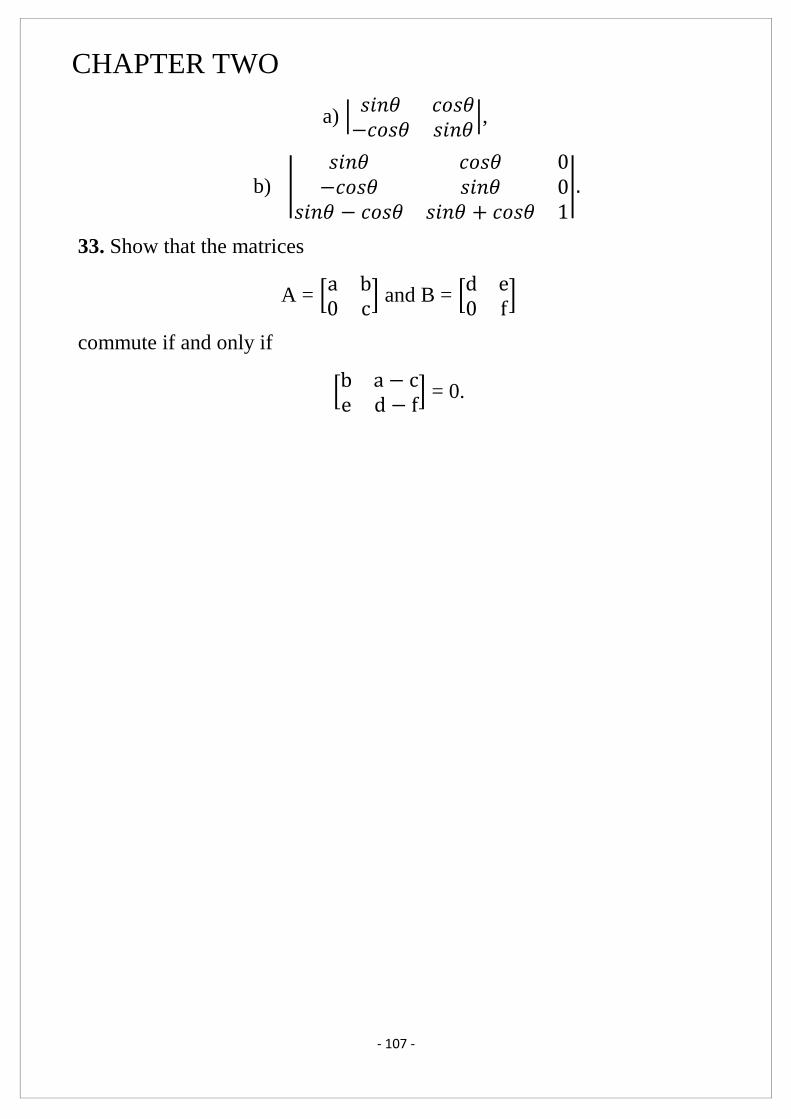
CHAPTER TWO
- 107 -
a) |𝑠𝑖𝑛𝜃 𝑐𝑜𝑠𝜃−𝑐𝑜𝑠𝜃 𝑠𝑖𝑛𝜃
|,
b) |𝑠𝑖𝑛𝜃 𝑐𝑜𝑠𝜃 0−𝑐𝑜𝑠𝜃 𝑠𝑖𝑛𝜃 0
𝑠𝑖𝑛𝜃 − 𝑐𝑜𝑠𝜃 𝑠𝑖𝑛𝜃 + 𝑐𝑜𝑠𝜃 1|.
33. Show that the matrices
A = [a b0 c
] and B = [d e0 f
]
commute if and only if
[b a − ce d − f
] = 0.

CHAPTER TWO
- 108 -
2.2 Evaluating Determinants by Row Reduction
THEOREM 2.2.1 Let A be a square matrix. If A has a row of zeros or a
column of
zeros, then det(A) = 0.
THEOREM 2.2.2 Let A be a square matrix. Then det(A) = det(AT ).
THEOREM 2.2.3 Let A be an n × n matrix.
(a) If B is the matrix that results when a single row or single column of A
is multiplied by a scalar k, then det(B) = k det(A).
(b) If B is the matrix that results when two rows or two columns of A are
interchanged, then det(B) = − det(A).
(c) If B is the matrix that results when a multiple of one row of A is added
to another or when a multiple of one column is added to another, then
det(B) = det(A).
THEOREM 2.2.4 Let E be an n × n elementary matrix.
(a) If E results from multiplying a row of In by a nonzero number k, then
det(E) = k.
(b) If E results from interchanging two rows of In, then det(E) = −1.
(c) If E results from adding a multiple of one row of In to another, then
det(E) = 1

CHAPTER TWO
- 109 -
EXAMPLE 1 Determinants of Elementary Matrices
|
1 0 0 00 3 0 00 0 1 00 0 0 1
| = 3, |
0 0 0 10 1 0 00 0 1 01 0 0 0
| = −1, |
1 0 0 70 1 0 00 0 1 00 0 0 1
| = 1.
THEOREM 2.2.5 If A is a square matrix with two proportional rows or
two proportional columns, then det(A) = 0.
EXAMPLE 2 Proportional Rows or Columns
Each of the following matrices has two proportional rows or columns;
thus, each has a determinant of zero.
[−1 4−2 8
], [1 −2 7−4 8 52 −4 3
], [
3 −1 4 − 56 −2 5 25 8 1 4
−9 3 − 12 15
].
EXAMPLE 3 Using Row Reduction to Evaluate a Determinant
Evaluate det(A) where
A = [0 1 53 −6 92 6 1
].
Solution We will reduce A to row echelon form (which is upper triangular)
and then apply Theorem 2.1.2.
det(A) = |0 1 53 −6 92 6 1
| = − |3 −6 90 1 52 6 1
|
= −3 |1 −2 30 1 52 6 1
|

CHAPTER TWO
- 110 -
= −3 |1 −2 30 1 50 10 −5
|
= −3 |1 −2 30 1 50 0 −55
|
= (−3)(−55) |1 −2 30 1 50 0 1
|
= (−3)(−55)(1) = −165.
EXAMPLE 4 Using Column Operations to Evaluate a Determinant
Compute the determinant of
A = [
1 0 0 32 7 0 60 6 3 0
7 3 1 − 5
].
Solution This determinant could be computed as above by using
elementary row operations to reduce A to row echelon form, but we can
put A in lower triangular form in one step by adding −3 times the first
column to the fourth to obtain
det(A) = det[
1 0 0 02 7 0 00 6 3 0
7 3 1 − 26
] = (1)(7)(3)( −26) = −546.
EXAMPLE 5 Row Operations and Cofactor Expansion
Evaluate det(A) where

CHAPTER TWO
- 111 -
A = [
3 5 −2 61 2 −1 12 4 1 53 7 5 3
].
Solution By adding suitable multiples of the second row to the remaining
rows, we
obtain
det(A) = |
0 −1 1 31 2 −1 10 0 3 30 1 8 0
|
= − |−1 1 30 3 31 8 0
|
= − |−1 1 30 3 30 9 3
|
= −(−1) |3 39 3
|
= −18.

CHAPTER TWO
- 112 -
Exercise Set 2.2
In Exercises 1–4, verify that det(A) = det(AT ).
1. A = [−2 31 4
] 2. A = [−6 12 −2
]
3.A = [2 −1 31 2 45 −3 6
] 4. A = [4 2 −10 2 −3−1 1 5
].
In Exercises 5–8, find the determinant of the given elementary matrix by
inspection
5. [
3 5 −2 61 2 −1 12 4 1 53 7 5 3
] 6. [1 0 00 1 0−5 0 1
]
7. [
1 0 0 00 0 1 00 1 0 00 0 0 1
] 8.
[
1 0 0 00 −1/3 0 00 0 1 00 0 0 1
].
In Exercises 9–13, evaluate the determinant of the matrix by first reducing
the matrix to row echelon form and then using some combination of row
operations and cofactor expansion
9. [3 −6 9−2 7 −20 1 5
] 10. [3 6 −90 0 −2−2 1 5
]
11. [
2 1 3 11 0 1 10 2 1 00 1 2 3
] 12. [1 −3 0−2 4 15 −2 2
]

CHAPTER TWO
- 113 -
13.
[ 1 3 1 5 3−2 −7 0 − 4 20 0 1 0 10 0 2 1 10 0 0 1 1]
.
In Exercises 14–21, evaluate the determinant, given that
|
𝑎 𝑏 𝑐𝑑 𝑒 𝑓𝑔 ℎ 𝑖
| = 6.
14. |d e fg h ia b c
| 15. |𝑔 ℎ 𝑖𝑑 𝑒 𝑓𝑎 𝑏 𝑐
|
16. |3a 3b 3c−d −e −f4g 4h 4i
| 17. |a + d b + e c + f−d −e −fg h i
|
18. |
a + g b + h c + id e fg h i
| 19. |
𝑎 𝑏 𝑐2𝑑 2𝑒 2𝑓
𝑔 + 3𝑎 ℎ + 3𝑏 𝑖 + 3𝑐|
20. |−3a −3b −3cd e f
g − 4d h − 4e i − 4f| 21. |
𝑎 𝑏 𝑐𝑑 𝑒 𝑓2𝑎 2𝑏 2𝑐
|.
22. Use row reduction to show that
|1 1 1𝑎 𝑏 𝑐𝑎2 𝑏2 𝑐2
| = (b−a)(c−a)(c−b).
23. Verify the formulas in parts (a) and (b) and then make a conjecture
about a general result of which these results are special cases

CHAPTER TWO
- 114 -
(a) det [0 0 𝑎130 𝑎22 𝑎23𝑎31 𝑎32 𝑎33
] = −𝑎13𝑎22𝑎31.
(b) det [
0 0 0 𝑎140 0 𝑎23 𝑎240 𝑎32 𝑎32 𝑎33𝑎41 𝑎42 𝑎43 𝑎44
] = 𝑎14𝑎23𝑎32𝑎41.
In Exercises 24–25, confirm the identities without evaluating the
determinants directly.
24. |
𝑎1 𝑏1 𝑎1 + 𝑏1 + 𝑐1𝑎2 𝑏2 𝑎2 + 𝑏2 + 𝑐2𝑎3 𝑏3 𝑎3 + 𝑏3 + 𝑐3
| = |
𝑎1 𝑏1 𝑐1𝑎2 𝑏2 𝑐2𝑎3 𝑏3 𝑐3
|.
25. |
𝑎1 + 𝑏1 𝑎1 − 𝑏1 𝑐1𝑎2 + 𝑏2 𝑎2 − 𝑏2 𝑐2𝑎3 + 𝑏3 𝑎3 − 𝑏3 𝑐3
| = −2|
𝑎1 𝑏1 𝑐1𝑎2 𝑏2 𝑐2𝑎3 𝑏3 𝑐3
|.

CHAPTER TWO
- 115 -
2.3 Properties of Determinants; Cramer’s Rule
Suppose that A and B are n × n matrices and k is any scalar. We
have
det (kA) = kn det(A).
EXAMPLE, 1 det (A + B) ≠ det (A) + det (B)
Consider
A = [1 22 5
], B = [3 11 3
], A + B =[4 33 8
].
We have det (A) = 1, det (B) = 8, det (A+B) = 23 ≠ det (A) + det (B).
THEOREM 2.3.1 Let A, B, and C be n × n matrices that differ only in a
single row, say the rth
, and assume that the rth
row of C can be obtained by
adding corresponding entries in the rth rows of A and B. Then
det(C) = det(A) + det(B)
The same result holds for columns.
EXAMPLE, 2 Sums of Determinants
det [1 7 52 0 3
1 + 0 4 + 1 7 + (−1)]= det [
1 7 52 0 31 4 7
]+ det [1 7 52 0 30 1 −1
]
THEOREM 2.3.2 A square matrix A is invertible if and only if det (A) ≠
0.
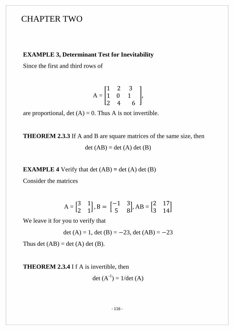
CHAPTER TWO
- 116 -
EXAMPLE 3, Determinant Test for Inevitability
Since the first and third rows of
A = [1 2 3 1 0 1 2 4 6
],
are proportional, det (A) = 0. Thus A is not invertible.
THEOREM 2.3.3 If A and B are square matrices of the same size, then
det (AB) = det (A) det (B)
EXAMPLE 4 Verify that det (AB) = det (A) det (B)
Consider the matrices
A = [3 12 1
] , B = [−1 35 8
], AB = [2 173 14
]
We leave it for you to verify that
det (A) = 1, det (B) = −23, det (AB) = −23
Thus det (AB) = det (A) det (B).
THEOREM 2.3.4 I f A is invertible, then
det (A-1
) = 1/det (A)

CHAPTER TWO
- 117 -
EXAMPLE 5 Entries and Cofactors from Different Rows
Let
A = [3 2 −1 1 6 3 2 −4 0
].
We leave it for you to verify that the cofactors of A are
C11 = 12, C12 = 6, C13 = −16
C21 = 4, C22 = 2, C23 = 16
C31 = 12, C32 = −10, C33 = 16.
So, for example, the cofactor expansion of det (A) along the first row is
det (A) = 3C11 + 2C12 + (−1)C13 = 36 + 12 + 16 = 64.
And along the first column is
det (A) = 3C11 + C21 + 2C31 = 36 + 4 + 24 = 64.
DEFINITION 1 If A is any n × n matrix and Cij is the cofactor of aij, then
the matrix
[ C11 C12 C1nC21 C22 C2n
Cn1 Cn2 Cnn] ,
is called the matrix of cofactors from A. The transpose of this matrix is
called the adjoint of A and is denoted by adj(A).
EXAMPLE 6 Adjoint of a 3 × 3 Matrix
Let

CHAPTER TWO
- 118 -
A = [3 2 −1 1 6 3 2 −4 0
].
As noted in Example 5, the cofactors of A are
C11 = 12, C12 = 6, C13 = −16
C21 = 4, C22 = 2, C23 = 16
C31 = 12, C32 = −10, C33 = 16,
so the matrix of cofactors is
[12 6 −16 4 2 16 12 −10 16
]
and the adjoint of A is
[12 4 12 6 2 −10 −16 16 16
].
THEOREM 2.3.5 Inverse of a Matrix Using Its Adjoint
If A is an invertible matrix, then
A-1
= 1
det(𝐴) adj (A)
EXAMPLE 7 Using the Adjoint to Find an Inverse Matrix
Find the inverse of the matrix A in Example 6.
We showed in Example 5 that det (A) = 64. Thus
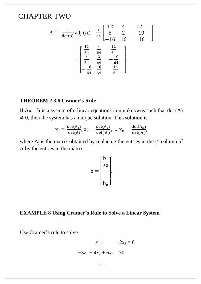
CHAPTER TWO
- 119 -
A-1
= 1
det(𝐴) adj (A) =
1
64 [12 4 12 6 2 −10 −16 16 16
]
=
[ 12
64
4
64
12
64
6
64
2
64 −
10
64
−16
64
16
64
16
64 ]
.
THEOREM 2.3.6 Cramer’s Rule
If Ax = b is a system of n linear equations in n unknowns such that det (A)
≠ 0, then the system has a unique solution. This solution is
x1 = det(A1)
det(A), x2 =
det(A2)
det( A ), … xn =
det(An)
det( A ),
where Aj is the matrix obtained by replacing the entries in the jth
column of
A by the entries in the matrix
b =
[ b1b2
bn ]
.
EXAMPLE 8 Using Cramer’s Rule to Solve a Linear System
Use Cramer’s rule to solve
x1+ +2x3 = 6
−3x1 + 4x2 + 6x3 = 30

CHAPTER TWO
- 120 -
−x1 − 2x2 + 3x3 = 8.
𝐴 = [1 0 2 −3 4 6 −1 −2 3
], A1 = [6 0 2 30 4 6 8 −2 3
]
A2 =[1 6 2 −3 30 6 −1 8 3
], A3 = [1 0 6 −3 4 30 −1 −2 8
].
x1 = det(A1)
det(A)=
−40
44=−10
11 , x2 =
det(A2)
det( A )=72
44=18
11,
x3 =det(A3)
det( A )=152
44 = 38
11.
THEOREM 2.3.7 Equivalent Statements
If A is an n × n matrix, then the following statements are equivalent.
(a) A is invertible.
(b) Ax = 0 has only the trivial solution.
(c) The reduced row echelon form of A is In.
(d) A can be expressed as a product of elementary matrices.
(e) Ax = b is consistent for every n × 1 matrix b.
(f) Ax = b has exactly one solution for every n × 1 matrix b.
(g) det (A) ≠ 0.
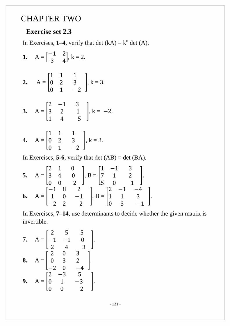
CHAPTER TWO
- 121 -
Exercise set 2.3
In Exercises, 1–4, verify that det (kA) = kn det (A).
1. A = [−1 23 4
], k = 2.
2. A = [1 1 1 0 2 3 0 1 −2
], k = 3.
3. A = [2 −1 3 3 2 1 1 4 5
], k = −2.
4. A = [1 1 1 0 2 3 0 1 −2
], k = 3.
In Exercises, 5-6, verify that det (AB) = det (BA).
5. A = [2 1 0 3 4 0 0 0 2
], B = [1 −1 3 7 1 2 5 0 1
].
6. A = [−1 8 2 1 0 −1 −2 2 2
], B = [2 −1 −4 1 1 3 0 3 −1
].
In Exercises, 7–14, use determinants to decide whether the given matrix is
invertible.
7. A = [2 5 5 −1 −1 0 2 4 3
].
8. A = [2 0 3 0 3 2 −2 0 −4
].
9. A = [2 −3 5 0 1 −3 0 0 2
].
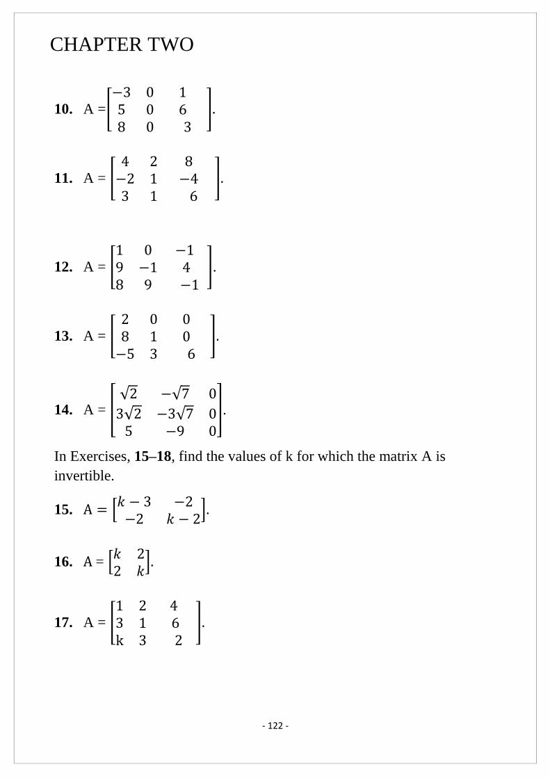
CHAPTER TWO
- 122 -
10. A =[−3 0 1 5 0 6 8 0 3
].
11. A = [4 2 8 −2 1 −4 3 1 6
].
12. A = [1 0 −1 9 −1 4 8 9 −1
].
13. A = [2 0 0 8 1 0 −5 3 6
].
14. A = [√2 −√7 0
3√2 −3√7 05 −9 0
].
In Exercises, 15–18, find the values of k for which the matrix A is
invertible.
15. A = [𝑘 − 3 −2−2 𝑘 − 2
].
16. A = [𝑘 22 𝑘
].
17. A = [1 2 4 3 1 6 k 3 2
].

CHAPTER TWO
- 123 -
18. A = [1 2 0 𝑘 1 𝑘 0 2 1
].
In Exercises, 19–22, decide whether the matrix is invertible, and if so, use
the adjoint method to find its inverse.
19. A = [2 5 5 −1 −1 0 2 4 3
].
20. A = [2 0 3 0 3 2 −2 0 −4
].
21. A = [2 −3 5 0 1 −3 0 0 2
].
22. A = [2 0 0 8 1 0 −5 3 6
].
In Exercises, 23–27, solve by Cramer’s rule, where it applies.
23. 7x1 – 2x2 =3 3x1 + x2 = 5.
24. x1 –3x2 +x3 = 4 2x1 –x2 = –2 4x1 –3x3 = 0.
25. 3x1 –x2 + x3 = 4 –x1 + 7x2 –2x3 = 1 2x1 +6x2 –x3 = 5.
26. 4x + 5y = 2 11x + y + 2z = 3 x + 5y + 2z = 1.
27. x − 4y + z = 6 4x − y + 2z = −1 2x + 2y − 3z = −20
28. Show that the matrix
[cos θ sin θ 0 −sinθ cos θ 0 0 0 1
],
is invertible for all values of θ; then find A-1
using the adjoint method.
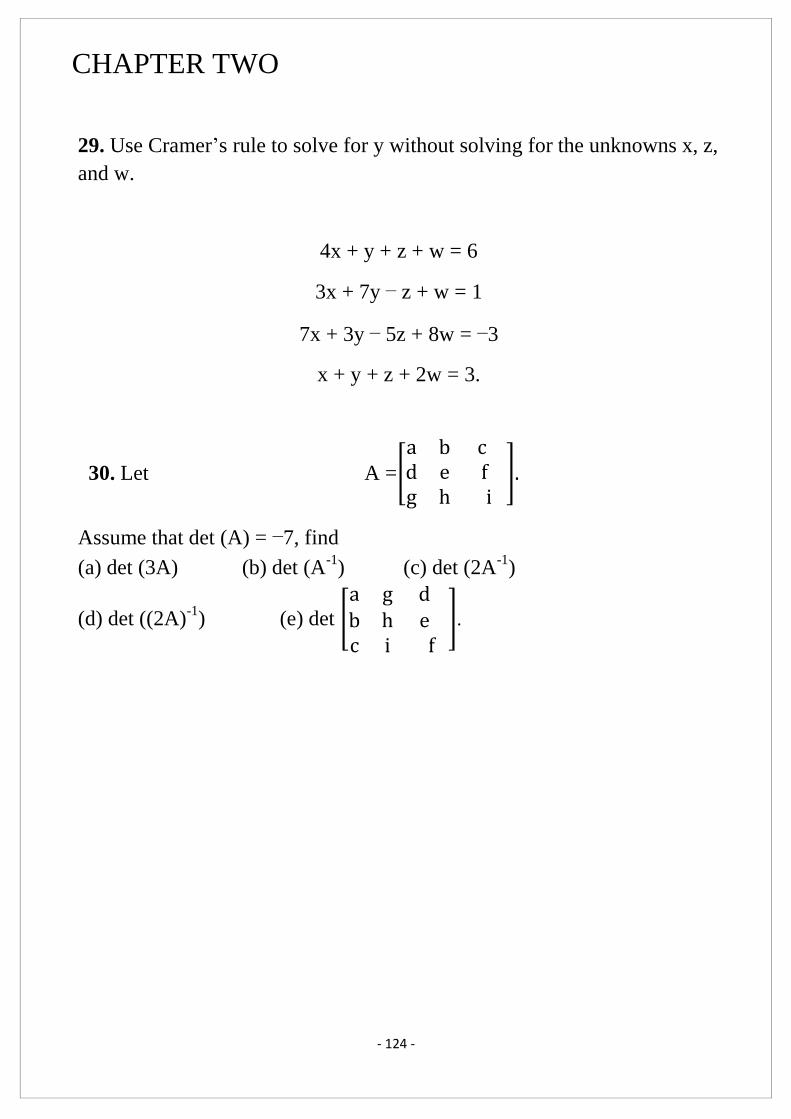
CHAPTER TWO
- 124 -
29. Use Cramer’s rule to solve for y without solving for the unknowns x, z,
and w.
4x + y + z + w = 6
3x + 7y − z + w = 1
7x + 3y − 5z + 8w = −3
x + y + z + 2w = 3.
30. Let A =[a b c d e f g h i
].
Assume that det (A) = −7, find
(a) det (3A) (b) det (A-1
) (c) det (2A-1
)
(d) det ((2A)-1
) (e) det [a g d b h e c i f
].

CHAPTER TWO
- 125 -
2.4 Vectors in 2-Space, 3-Space, and n-Space
Parallelogram Rule for Vector Addition If v and w are vectors in 2-
space or 3-space that are positioned so their initial points coincide, then the
two vectors form adjacent sides of a parallelogram, and the sum v + w is
the vector represented by the arrow from the common initial point of v and
w to the opposite vertex of the parallelogram (Figure 6.1a).
Triangle Rule for Vector Addition If v and w are vectors in 2-space or 3-
space that are positioned so the initial point of w is at the terminal point of
v, then the sum v + w is represented by the arrow from the initial point of v
to the terminal point of w (Figure 2.4.1b).
Figure 2.4.1
(a) (b)
Generally, v + w = w + v.
Vector Subtraction. The negative of a vector v, denoted by −v, is the vector
that has the same length as v but is oppositely directed (Figure 2.4.1a), and
the difference of v from w, denoted by w − v, is taken to be the sum w − v
= w + (−v).
The difference of v from w can be obtained geometrically by the
parallelogram method shown in Figure 2.4.1b.
v + w
w
w
v + w

CHAPTER TWO
- 126 -
Figure 2.4.2
(a) (b)
Scalar Multiplication If v is a nonzero vector in 2-space or 3-space, and if
k is a nonzero scalar, then we define the scalar product of v by k to be the
vector whose length is |k| times the length of v and whose direction is the
same as that of v if k is positive and opposite to that of v if k is negative. If
k = 0 or v = 0, then we define kv to be 0.
Note that
(−1) v = −v.
Vector addition satisfies the associative law for addition, meaning that
when we add three vectors, say u, v, and w, it does not matter which two
we add first; that is,
u + (v + w) = (u + v) + w
If a vector v in 2-space or 3-space is positioned with its initial point at the
origin of a rectangular coordinate system, then the vector is completely
determined by the coordinates of its terminal point (Figure 2.4.3). We call
these coordinates the components of v relative to the coordinate system.
We will write v = (v1, v2) to denote a vector v in 2-space with components
(v1, v2), and v = (v1, v2, v3) to denote a vector v in 3-space with
components (v1, v2, v3).
w – vThe
w

CHAPTER TWO
- 127 -
Figure 2.4.3
The vectors
v = (v1, v2, v3) and w = (w1, w2, w3)
in 3-space are equivalent if and only if
v1 = w1, v2 = w2, v3 = w3.
It is sometimes necessary to consider vectors whose initial points are not at
the origin. If 𝐩𝟏𝐩𝟐⃗⃗ ⃗⃗ ⃗⃗ ⃗⃗ ⃗⃗ denotes the vector with initial point P1(x1, y1) and
terminal point P2(x2, y2), then the components of this vector are given by
the formula
𝐩𝟏𝐩𝟐⃗⃗ ⃗⃗ ⃗⃗ ⃗⃗ ⃗⃗ = (x2 − x1, y2 − y1).
As you might expect, the components of a vector in 3-space that has initial
point p1(x1, y1, z1) and terminal point p2(x2, y2, z2) are given by
𝐩𝟏𝐩𝟐⃗⃗ ⃗⃗ ⃗⃗ ⃗⃗ ⃗⃗ = (x2 − x1, y2 − y1, z2 − z1).
EXAMPLE 1 Finding the Components of a Vector
The components of the vector v = 𝐩𝟏𝐩𝟐⃗⃗ ⃗⃗ ⃗⃗ ⃗⃗ ⃗⃗ with initial point P1(2,−1, 4) and
terminal point P2(7, 5,−8) are
(v1, v2)
v
x
v
z
(v1, v2, v3)
x

CHAPTER TWO
- 128 -
v = (7 − 2, 5 − (−1), (−8) − 4) = (5, 6,−12).
DEFINITION 1 If n is a positive integer, then an ordered n-tuple is a
sequence of n real numbers (v1, v2, . . . , vn). The set of all ordered n-tuples
is called n-space and is denoted by Rn.
Our next goal is to define useful operations on vectors in Rn. These
operations will all be natural extensions of the familiar operations on
vectors in R2 and R
3. We will denote a vector v in R
n using the notation
v = (v1, v2, . . . , vn),
and we will call 0 = (0, 0, . . . , 0) the zero vector.
DEFINITION 2 Vectors v = (v1, v2, . . . , vn) and w = (w1, w2, . . . , wn) in Rn
are said to be equivalent (also called equal) if
v1 = w1, v2 = w2, . . . , vn = wn
We indicate this by writing v = w.
EXAMPLE 2 Equality of Vectors
(a, b, c, d) = (1,−4, 2, 7),
if and only if a = 1, b = −4, c = 2, and d = 7.
DEFINITION 3 If v = (v1, v2, . . . , vn) and w = (w1, w2, . . . , wn) are
vectors in Rn, and if k is any scalar, then we define
v + w = (v1 + w1, v2 + w2, . . . , vn + wn).
kv = (kv1, kv2, . . . , kvn).

CHAPTER TWO
- 129 -
−v = (−v1,−v2, . . . ,−vn).
w − v = w + (−v) = (w1 − v1 , w2 − v2, . . . , wn − vn).
EXAMPLE 3 Algebraic Operations Using Components
If v = (1,−3, 2) and w = (4, 2, 1), then
v + w = (5,−1, 3), 2v = (2,−6, 4)
−w = (−4,−2,−1), v − w = v + (−w) = (−3,−5, 1).
THEOREM 2.4.1 If u, v, and w are vectors in Rn, and if k and m are scalars,
then:
(a) u + v = v + u
(b) (u + v) + w = u + (v + w)
(c) u + 0 = 0 + u = u
(d) u + (−u) = 0
(e) k(u + v) = ku + kv
(f) (k + m)u = ku + mu
(g) k(mu) = (km)u
(h) 1u = u.
THEOREM 2.4.2 If v is a vector in Rn and k is a scalar, then:
(a) 0v = 0
(b) k0 = 0
CHAPTER TWO
- 130 -
(c) 1 (−1)v = −v.
DEFINITION 4 If w is a vector in Rn, then w is said to be a linear
combination of the vectors v1, v2, . . . , vr in Rn if it can be expressed in the
form
w = k1v1 + k2v2 +· · ·+kr vr
where k1, k2, . . . , kr are scalars. These scalars are called the coefficients of
the linear combination. In the case where r = 1, the formula becomes w =
k1v1, so that a linear combination of a single vector is just a scalar multiple
of that vector.
Any vector v = (v1, v2, . . . , vn) can be written as
v = [v1, v2, . . . , vn],
which is called row-vector form, or as
v =
[ 𝑣1𝑣2
𝑣𝑛 ]
,
which is called column-vector form.

CHAPTER TWO
- 131 -
Exercise set 2.4
In Exercises, 1–2, find the components of the vector 𝐩𝟏𝐩𝟐⃗⃗ ⃗⃗ ⃗⃗ ⃗⃗ ⃗⃗ .
1. (a) P1(3, 5), P2(2, 8) (b) P1(5,−2, 1), P2(2, 4, 2)
2. (a) P1(−6, 2), P2(−4,−1) (b) P1(0, 0, 0), P2(−1, 6, 1).
3. (a) Find the terminal point of the vector that is equivalent to
u = (1, 2) and whose initial point is A(1, 1).
(b) Find the initial point of the vector that is equivalent to
u = (1, 1, 3) and whose terminal point is B(−1,−1, 2).
4. (a) Find the initial point of the vector that is equivalent to
u = (1, 2) and whose terminal point is B(2, 0).
(b) Find the terminal point of the vector that is equivalent to
u = (1, 1, 3) and whose initial point is A(0, 2, 0).
5. Find an initial point P of a nonzero vector u =𝑷𝐐⃗⃗⃗⃗⃗⃗ . with terminal
point Q(3, 0,−5) and such that
(a) u has the same direction as v = (4,−2,−1).
(b) u is oppositely directed to v = (4,−2,−1).
6. Find a terminal point Q of a nonzero vector u =𝑷𝑸⃗⃗⃗⃗⃗⃗ with initial point
P(−1, 3,−5) and such that
(a) u has the same direction as v = (6, 7,−3).
(b) u is oppositely directed to v = (6, 7,−3).
7. Let u = (4,−1), v = (0, 5), and w = (−3,−3). Find the components of

CHAPTER TWO
- 132 -
(a) u + w (b) v − 3u
(c) 2(u − 5w) (d) 3v − 2(u + 2w).
8. Let u = (−3, 1, 2), v = (4, 0, −8), and w = (6, −1, −4). Find the
components of
(a) v − w (b) 6u + 2v
(c) −3(v − 8w) (d) (2u − 7w) − (8v + u).
9. Let u = (−3, 2, 1, 0), v = (4, 7, −3, 2), and w = (5, −2, 8, 1). Find the
components of
(a) v − w (b) −u + (v − 4w)
(c) 6(u − 3v) (d) (6v − w) − (4u + v)
10. Let u = (1, 2, -3, 5, 0), v = (0, 4, -1, 1, 2), and w = (7, 1, −4−2, 3) be.
Find the components of
(a) v + w, (b) 3(2u − v)
(c) (3 u − v) − (2u + 4 w), (d) ½(w−5v+2u) + v
11. Let u, v, and w be the vectors in Exercise 9. Find the components of the
vector x that satisfies the equation
3u + v − 2w = 3x + 2w.
12.Let u, v, and w be the vectors in Exercise 10. Find the components of the
vector x that satisfies the equation
2u − v + x = 7x + w.
13. Which of the following vectors in R6, if any, are parallel to u = (−2,1, 0, 3,
5, 1)?
(a) (4, 2, 0, 6, 10, 2)
(b) (4, −2, 0, −6, −10, −2) (c) (0, 0, 0, 0, 0, 0).
14. For what value(s) of t, if any, is the given vector parallel to u = (4, −1)?

CHAPTER TWO
- 133 -
(a) (8t, −2) (b) (8t, 2t) (c) (1, t2).
15. Let u = (1, −1, 3, 5) and v = (2, 1, 0, −3). Find scalars a and b so that
au + bv = (1, −4, 9, 18).
In Exercises, 16–17, find scalars c1, c2, and c3 for which the equation is
satisfied
16.c1(1, −1, 0) + c2(3, 2, 1) + c3(0, 1, 4) = (−1, 1, 19).
17.c1(−1, 0, 2) + c2(2, 2, −2) + c3(1, −2, 1) = (−6, 12, 4).
18. Show that there do not exist scalars c1, c2, and c3 such that
c1(−2, 9, 6) + c2(−3, 2, 1) + c3(1, 7, 5) = (0, 5, 4).

CHAPTER TWO
- 134 -
2.5 Norm, Dot Product, and Distance in Rn
We will denote the length of a vector v by the symbol‖v‖, which is read as
the norm of v, the length of v, or the magnitude of v. the norm of a vector
(v1, v2) in R2 is
‖𝑣‖ = √𝑣12 + 𝑣2
2.
Similarly, for a vector (v1, v2, v3) in R3, we have
‖𝑣‖ = √𝑣12 + 𝑣2
2 + 𝑣32.
DEFINITION 1 If v = (v1, v2, . . . , vn) is a vector in Rn, then the norm of
v (also called the length of v or the magnitude of v) is denoted by‖𝐯‖,
and is defined by the formula
‖v‖ = √v12 + v2
2 +⋯+ vn2
EXAMPLE 1 Calculating Norms
The norm of the vector v = (−3, 2, 1) in R3 is
‖v‖ = √(−3)2 + 22 + 12 = √14.
The norm of the vector v = (2, −1, 3, −5) in R4 is
‖v‖ = √(2)2 + (−1)2 + 32 + (−5)2 = √39.
Our first theorem in this section will generalize to Rn the following three
familiar facts about vectors in R2 and R
3:
• Distances are nonnegative.
• The zero vector is the only vector of length zero.
• Multiplying a vector by a scalar multiplies its length by the absolute
value of that scalar
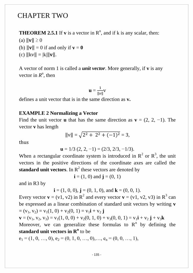
CHAPTER TWO
- 135 -
THEOREM 2.5.1 If v is a vector in Rn, and if k is any scalar, then:
(a) ‖𝐯‖ ≥ 0
(b) ‖𝐯‖ = 0 if and only if v = 0
(c) ‖kv‖ = |k|‖𝐯‖.
A vector of norm 1 is called a unit vector. More generally, if v is any
vector in Rn, then
u = 1
‖𝑣‖v
defines a unit vector that is in the same direction as v.
EXAMPLE 2 Normalizing a Vector
Find the unit vector u that has the same direction as v = (2, 2, −1). The
vector v has length
‖v‖ = √22 + 22 + (−1)2 = 3,
thus
u = 1/3 (2, 2, −1) = (2/3, 2/3, −1/3).
When a rectangular coordinate system is introduced in R2 or R
3, the unit
vectors in the positive directions of the coordinate axes are called the
standard unit vectors. In R2 these vectors are denoted by
i = (1, 0) and j = (0, 1)
and in R3 by
i = (1, 0, 0), j = (0, 1, 0), and k = (0, 0, 1).
Every vector v = (v1, v2) in R2 and every vector v = (v1, v2, v3) in R
3 can
be expressed as a linear combination of standard unit vectors by writing v
= (v1, v2) = v1(1, 0) + v2(0, 1) = v1i + v2 j
v = (v1, v2, v3) = v1(1, 0, 0) + v2(0, 1, 0) + v3(0, 0, 1) = v1i + v2 j + v3k
Moreover, we can generalize these formulas to Rn by defining the
standard unit vectors in Rn to be
e1 = (1, 0, …, 0), e2 = (0, 1, 0, …, 0),…, en = (0, 0, …, 1),
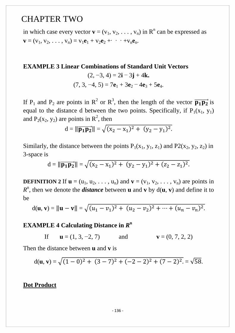
CHAPTER TWO
- 136 -
in which case every vector v = (v1, v2, . . . , vn) in Rn can be expressed as
v = (v1, v2, . . . , vn) = v1e1 + v2e2 +· · ·+vnen.
EXAMPLE 3 Linear Combinations of Standard Unit Vectors
(2, −3, 4) = 2i − 3j + 4k.
(7, 3, −4, 5) = 7e1 + 3e2 − 4e3 + 5e4.
If P1 and P2 are points in R2 or R
3, then the length of the vector 𝐩𝟏𝐩𝟐⃗⃗ ⃗⃗ ⃗⃗ ⃗⃗ ⃗⃗ is
equal to the distance d between the two points. Specifically, if P1(x1, y1)
and P2(x2, y2) are points in R2, then
d = ‖𝐩𝟏𝐩𝟐⃗⃗ ⃗⃗ ⃗⃗ ⃗⃗ ⃗⃗ ‖ = √(x2 − x1)2 + (y2 − y1)
2.
Similarly, the distance between the points P1(x1, y1, z1) and P2(x2, y2, z2) in
3-space is
d = ‖𝐩𝟏𝐩𝟐⃗⃗ ⃗⃗ ⃗⃗ ⃗⃗ ⃗⃗ ‖ = √(x2 − x1)2 + (y2 − y1)
2 + (𝑧2 − 𝑧1)2.
DEFINITION 2 If u = (u1, u2, . . . , un) and v = (v1, v2, . . . , vn) are points in
Rn, then we denote the distance between u and v by d(u, v) and define it to
be
d(u, v) = ‖𝐮 − 𝐯‖ = √(𝑢1 − 𝑣1)2 + (𝑢2 − 𝑣2)
2 +⋯+ (𝑢𝑛 − 𝑣𝑛)2.
EXAMPLE 4 Calculating Distance in Rn
If u = (1, 3, −2, 7) and v = (0, 7, 2, 2)
Then the distance between u and v is
d(u, v) = √(1 − 0)2 + (3 − 7)2 + (−2 − 2)2 + (7 − 2)2. = √58.
Dot Product

CHAPTER TWO
- 137 -
DEFINITION 3 If u and v are nonzero vectors in R2 or R
3, and if θ is the
angle between u and v, then the dot product (also called the Euclidean
inner product) of u and v is denoted by u ・ v and is defined as
u ・ v = ‖𝒖‖‖𝒗‖ cos θ
If u = 0 or v = 0, then we define u ・ v to be 0.
The sign of the dot product reveals information about the angle θ that we
can obtain by rewriting last equation as
cos θ = 𝒖 ・ 𝒗
‖𝒖‖‖𝒗‖.
The properties of the cosine function studied in trigonometry that
θ is acute if u ・ v ≥ 0, θ is obtuse if u ・ v ≤ 0, θ = π/2 if u ・ v =
0.
EXAMPLE 5 Dot Product
Find the dot product of the vectors whose lengths are ‖𝒖‖ = 1, ‖𝒗‖ = √8
= 2√2.
Moreover, the angle between them is θ = 45°.
u ・ v = ‖𝐮‖‖𝐯‖ cos θ = (1)(2√2)(1/√2) = 2.
Let u = (u1, u2, u3) and v = (v1, v2, v3) be two nonzero vectors. We can
prove
u ・ v = u1v1 + u2v2 + u3v3.
The companion formula for vectors in 2-space is
CHAPTER TWO
- 138 -
u ・ v = u1v1 + u2v2.
DEFINITION 4
If u = (u1, u2, . . . , un) and v = (v1, v2, . . . , vn) are vectors in Rn, then the
dot product (also called the Euclidean inner product) of u and v is
denoted by u ・ v and is defined by
u ・ v = u1v1 + u2v2 +· · ·+unvn.
EXAMPLE 6 Calculating Dot Products Using Components
Calculate u ・ v for the following vectors in R4:
u = (−1, 3, 5, 7), v = (−3, −4, 1, 0).
u ・ v = (−1)(−3) + (3)(−4) + (5)(1) + (7)(0) = −4.
In the special case where u = v in Definition 4, we obtain the relationship
v ・ v = 𝑣12 + 𝑣2
2 +⋯+ 𝑣𝑛2 = ‖𝐯‖2,
hence, we deduce
‖𝐯‖ = √𝐯 ・ 𝐯.
THEOREM 2.5.2 If u, v, and w are vectors in Rn, and if k is a scalar,
then:
(a) u ・ v = v ・ u
(b) u ・ (v + w) = u ・ v + u ・ w
(c) k(u ・ v) = (ku) ・ v
(d) v ・ v ≥ 0 and v ・ v = 0 if and only if v = 0.
THEOREM 2.5.3 If u, v, and w are vectors in Rn, and if k is a scalar,
then:
CHAPTER TWO
- 139 -
(a) 0 ・ v = v ・ 0 = 0
(b) (u + v) ・ w = u ・ w + v ・ w
(c) u ・ (v − w) = u ・ v − u ・ w
(d) (u − v) ・ w = u ・ w − v ・ w
(e) k(u ・ v) = u ・ (kv).
EXAMPLE 7 Calculating with Dot Products
(u − 2v) ・ (3u + 4v) = u ・ (3u + 4v) − 2v ・ (3u + 4v)
= 3(u ・ u) + 4(u ・ v) − 6(v ・ u) − 8(v ・ v)
= 3‖𝐮‖𝟐 − 2(u ・ v) – 8‖𝐯‖𝟐.
From the definition of dot product, we deduce
θ = cos-1
𝐮 ・ 𝐯
‖𝒖‖‖𝑣‖
THEOREM 2.5.4 Cauchy–Schwarz Inequality
If u = (u1, u2, . . . , un) and v = (v1, v2, . . . , vn) are vectors in Rn, then
| u ・ v |≤ ‖𝐮‖‖v‖,
or in terms of components
| u1v1 + u2v2 +· · ·+unvn.| ≤ (u12 + u2
2 +⋯+ un2)1/2(v1
2 + v22 +⋯+
vn2)1/2
THEOREM 2.5.5 If u, v, and w are vectors in Rn, then:
(a) ‖𝐮 + 𝐯‖ ≤ ‖𝐮‖ + ‖𝐯‖
CHAPTER TWO
- 140 -
(b) d(u, v) ≤ d(u, w) + d(w, v)
THEOREM 2.5.6 Parallelogram Equation for Vectors
If u and v are vectors in Rn, then
‖𝒖 + 𝐯‖𝟐 + ‖𝐮 − 𝐯‖𝟐 = 2(‖𝐮‖𝟐 + ‖𝒗‖𝟐)
THEOREM 7.7 If u and v are vectors in Rn with the Euclidean inner
product, then
u ・ v = ¼(‖𝒖 + 𝐯‖𝟐 −‖𝐮 − 𝐯‖𝟐).

CHAPTER TWO
- 141 -
Exercise set 2.5
In Exercises, 1–2, find the norm of v, and a unit vector that is oppositely
directed to v.
1. (a) v = (2, 2, 2) (b) v = (1, 0, 2, 1, 3).
2. (a) v = (1, − 1, 2) (b) v = (−2, 3, 3, −1).
In Exercises, 3–4, evaluate the given expression with u = (2, −2, 3), v = (1,
−3, 4), and w = (3, 6, −4).
3. (a) ‖𝐮 + 𝐯‖ (b) ‖𝐮‖ + ‖𝐯‖
(c) ‖−2𝐮 + 2𝐯‖ (d) ‖3𝐮 − 5𝐯 + 𝐰‖.
4. (a) ‖𝐮 + 𝐯 + 𝐰‖ (b) ‖𝐮 − 𝐯‖
(c) ‖3𝐯‖ -3 ‖𝐯‖ (d) ‖𝐮‖ – ‖𝐯‖.
In Exercises, 5–6, evaluate the given expression with
u = (−2,−1,4,5), v = (3,1,−5,7), and w = (−6,2,1,1).
5. (a) ‖3𝐮 − 5𝐯 + 𝐰‖ (b) ‖3𝐮‖ – 5‖𝐯‖ + ‖𝐰‖.
(c) ‖−‖𝐮‖𝒗‖.
6. (a) ‖𝐮‖ + ‖−2𝐯‖ + ‖−3𝐰‖.
(b) ‖‖𝐮 − 𝐯‖𝒘‖.
7. Let v = (−2, 3, 0, 6). Find all scalars k such that ‖k𝐯‖ = 5.
8. Let v = (1, 1, 2, −3, 1). Find all scalars k such that ‖k𝐯‖ = 4.
In Exercises, 9–10, find u ・ v, u ・ u, and v ・ v.
9. (a) u = (3, 1, 4), v = (2, 2,−4)
10. (a) u = (1, 1, −2, 3), v = (−1, 0, 5, 1)
(b) u = (2, −1, 1, 0, −2), v = (1, 2, 2, 2, 1).
CHAPTER TWO
- 142 -
In Exercises, 11–12, find the Euclidean distance between u and v and the
cosine of the angle between those vectors. State whether that angle is
acute, obtuse, or 90◦.
11. (a) u = (3, 3, 3), v = (1, 0, 4)
(b) u = (0, −2, −1, 1), v = (−3, 2, 4, 4).
12. (a) u = (1, 2, −3, 0), v = (5, 1, 2, −2)
(b) u = (0, 1, 1, 1, 2), v = (2, 1, 0, −1, 3).
In Exercises, 13–14, determine whether the expression makes sense
mathematically. If not, explain why.
13. (a) u ・ (v ・ w) (b) u ・ (v + w)
(c) ‖𝒖 . 𝐯‖ (d) u . v – ‖𝐮‖.
14. (a) ‖𝐮‖ . ‖𝐯‖ (b) u . v – w
(c) u . v – k (d) k . u.
In Exercises, 15–16, verify that the Cauchy–Schwarz inequality holds.
15. (a) u = (−3, 1, 0), v = (2, −1, 3)
(b) u = (0, 2, 2, 1), v = (1, 1, 1, 1).
16. (a) u = (4, 1, 1), v = (1, 2, 3)
(b) u = (1, 2, 1, 2, 3), v = (0, 1, 1, 5, −2).
17. For a vector v = (v1, v2, v3) in R3, let the direction cosines be defined as
cos 𝛼 = 𝑣1
‖𝒗‖, cos 𝛽 =
𝑣2
‖𝒗‖ , cos 𝛾 =
𝑣3
‖𝒗‖.
Show that
𝑐𝑜𝑠2 𝛼 + 𝑐𝑜𝑠2 𝛽 + 𝑐𝑜𝑠2 𝛾 = 1.
CHAPTER TWO
- 143 -
2.6 Cross Product
DEFINITION 1 If u = (u1, u2, u3) and v = (v1, v2, v3) are vectors in 3-
space, then the cross product u × v is the vector defined by
u × v = (u2v3 − u3v2, u3v1 − u1v3, u1v2 − u2v1),
or, in determinant notation,
u × v = (|𝑢2 𝑢3𝑣2 𝑣3
| , − |𝑢1 𝑢3𝑣1 𝑣3
| , |𝑢1 𝑢2𝑣1 𝑣2
|)
EXAMPLE 1 Calculating a Cross Product
Find u × v, where u = (1, 2, −2) and v = (3, 0, 1).
u × v = (|2 −20 1
| , − |1 −23 1
| , |1 23 0
|)
(2, −7, −6).
THEOREM 2.6.1 Relationships Involving Cross Product and Dot
Product
If u, v, and w are vectors in 3-space, then
(a) u ・ (u × v) = 0
(b) v ・ (u × v) = 0
(c) ‖𝒖 × 𝒗‖𝟐 = ‖𝒖 ‖𝟐‖ 𝐯‖𝟐 −(u ・ v)2 (Lagrange’s Identity)
(d) u × (v × w) = (u ・ w) v − (u ・ v) w (vector triple product)
(e) (u × v )× w = (u ・ w) v − (v ・ w) u (vector triple product)
CHAPTER TWO
- 144 -
EXAMPLE 2
u × v is Perpendicular to u and to v
Consider the vectors
u = (1, 2, −2) and v = (3, 0, 1)
In Example 1, we showed that
u × v = (2, −7, −6).
Since
u ・ (u × v) = (1)(2) + (2)(−7) + (−2)(−6) = 0,
and
v ・ (u × v) = (3)(2) + (0)(−7) + (1)(−6) = 0,
u × v is orthogonal to both u and v.
THEOREM 2.6.2 Properties of Cross Product
If u, v, and w are any vectors in 3-space and k is any scalar, then:
(a) u × v = −(v × u)
(b) u × (v + w) = (u × v) + (u × w)
(c) (u + v) × w = (u × w) + (v × w)
(d) k(u × v) = (ku) × v = u × (kv)
(e) u × 0 = 0 × u = 0, (f) u × u = 0
EXAMPLE 3 Cross Products of the Standard Unit Vectors
Recall from Section 7 that the standard unit vectors in 3-space are
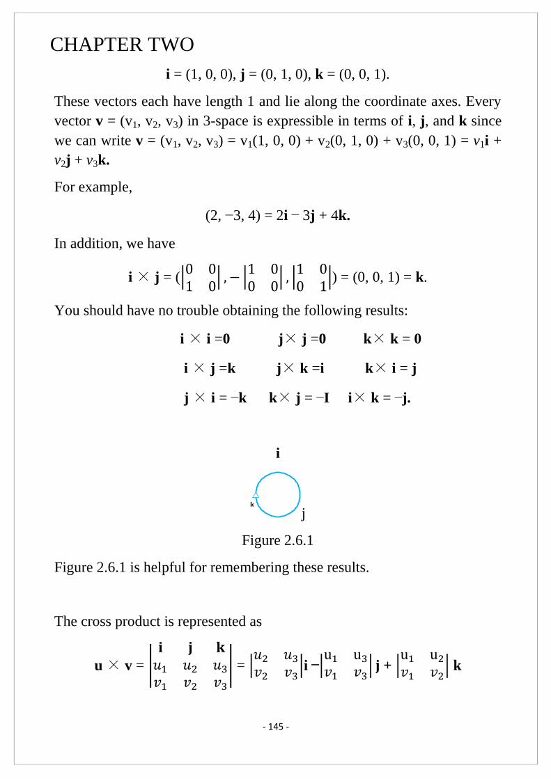
CHAPTER TWO
- 145 -
i = (1, 0, 0), j = (0, 1, 0), k = (0, 0, 1).
These vectors each have length 1 and lie along the coordinate axes. Every
vector v = (v1, v2, v3) in 3-space is expressible in terms of i, j, and k since
we can write v = (v1, v2, v3) = v1(1, 0, 0) + v2(0, 1, 0) + v3(0, 0, 1) = v1i +
v2j + v3k.
For example,
(2, −3, 4) = 2i − 3j + 4k.
In addition, we have
i × j = (|0 01 0
| , − |1 00 0
| , |1 00 1
|) = (0, 0, 1) = k.
You should have no trouble obtaining the following results:
i × i =0 j× j =0 k× k = 0
i × j =k j× k =i k× i = j
j × i = −k k× j = −I i× k = −j.
i
j
Figure 2.6.1
Figure 2.6.1 is helpful for remembering these results.
The cross product is represented as
u × v = |𝐢 𝐣 𝐤𝑢1 𝑢2 𝑢3𝑣1 𝑣2 𝑣3
| = |𝑢2 𝑢3𝑣2 𝑣3
|i −|u1 u3𝑣1 𝑣3
| 𝐣 + |u1 u2𝑣1 𝑣2
| k
k

CHAPTER TWO
- 146 -
For example, if u = (1, 2, −2) and v = (3, 0, 1), then
u × v = |𝐢 𝐣 𝐤1 2 −23 0 1
| = 2𝐢 – 7𝐣 – 6𝐤.
You may find it instructive to practice this rule with the products
i × j = k, j × k = i, k × i = j.
From Theorem (2.6.1) we have
‖𝒖 × 𝒗‖𝟐 = ‖𝒖 ‖𝟐‖ 𝐯‖𝟐 −(u ・ v)2 (I)
If θ denotes the angle between u and v, then u ・ v = ‖𝒖 ‖‖ 𝐯‖ cos θ, so
(I) can be written as
‖𝒖 × 𝒗‖𝟐 = ‖𝒖 ‖𝟐‖ 𝐯‖𝟐 −‖𝒖 ‖𝟐‖ 𝐯‖𝟐 cos2 θ
= ‖𝒖 ‖𝟐‖ 𝐯‖𝟐 (1−cos2 θ)
= ‖𝒖 ‖𝟐‖ 𝐯‖𝟐 sin2 θ,
which implies that
‖𝒖 × 𝒗‖ = ‖𝒖 ‖‖ 𝐯‖ sin θ.
THEOREM 2.6.3 Area of a Parallelogram
If u and v are vectors in 3-space, then ‖𝐮 × 𝐯‖ is equal to the area of the
parallelogram determined by u and v.
EXAMPLE 4 Area of a Triangle
Find the area of the triangle determined by the points P1(2, 2, 0), P2(−1, 0,
2), and P3(0, 4, 3).

CHAPTER TWO
- 147 -
The area A of the triangle is 1/2 the area of the parallelogram determined
by the vectors 𝐩𝟏𝐩𝟐⃗⃗ ⃗⃗ ⃗⃗ ⃗⃗ ⃗⃗ and 𝐩𝟏𝐩𝟑⃗⃗ ⃗⃗ ⃗⃗ ⃗⃗ ⃗⃗ ⃗. We have 𝐩𝟏𝐩𝟐⃗⃗ ⃗⃗ ⃗⃗ ⃗⃗ ⃗⃗ = (−3, −2, 2), 𝐩𝟏𝐩𝟑⃗⃗ ⃗⃗ ⃗⃗ ⃗⃗ ⃗⃗ ⃗ = (−2,
2, 3). It follows that
𝒑𝟏𝒑𝟐⃗⃗ ⃗⃗ ⃗⃗ ⃗⃗ ⃗⃗ × 𝒑𝟏𝒑𝟑⃗⃗ ⃗⃗ ⃗⃗ ⃗⃗ ⃗⃗ ⃗ = (−10, 5, −10),
and consequently that
A = ½ ‖𝒑𝟏𝒑𝟐⃗⃗ ⃗⃗ ⃗⃗ ⃗⃗ ⃗⃗ × 𝒑𝟏𝒑𝟑⃗⃗ ⃗⃗ ⃗⃗ ⃗⃗ ⃗⃗ ⃗ ‖ = 15/2.
DEFINITION 2 If u, v, and w are vectors in 3-space, then
u ・ (v × w),
is called the scalar triple product of u, v, and w.
The scalar triple product of u = (u1, u2, u3), v = (v1, v2, v3), and w = (w1,
w2, w3) can be calculated from the formula
u ・ (v × w) = |
u1 u2 u3𝑣1 𝑣2 𝑣3𝑤1 𝑤2 𝑤3
|.
EXAMPLE 5 Calculating a Scalar Triple Product
Calculate the scalar triple product u ・ (v × w) of the vectors
u = 3i − 2j − 5k, v = i + 4j − 4k, w = 3j + 2k
u ・ (v × w) = |3 −2 −51 4 −40 3 2
|,
= 3|4 −43 2
| − (−2) |1 −40 2
| + (−5) |1 40 3
|
= 60 + 4 − 15 = 49.

CHAPTER TWO
- 148 -
THEOREM 2.6.4
(a) The absolute value of the determinant
det [𝑢1 𝑢2𝑣1 𝑣2
],
is equal to the area of the parallelogram in 2-space determined by the
vectors u = (u1, u2) and v = (v1, v2).
(b) The absolute value of the determinant
det [
𝑢1 𝑢2 𝑢3𝑣1 𝑣2 𝑣3𝑤1 𝑤2 𝑤3
],
is equal to the volume of the parallelepiped in 3-space determined by the
vectors u = (u1, u2, u3), v = (v1, v2, v3), and w = (w1, w2, w3).

CHAPTER TWO
- 149 -
Exercise set 2.6
In Exercises 1–2, let u = (3, 2, −1), v = (0, 2, −3), and w = (2, 6, 7).
Compute the indicated vectors.
1. (a) v × w (b) w × v (c) (u + v) × w
(d) v ・ (v × w) (e) v × v (f) (u − 3w) × (u − 3w).
2. (a) u × v (b) −(u × v) (c) u × (v + w)
(d) w ・ (w × v) (e) w × w (f) (7v − 3u) × (7v − 3u).
In Exercises 3–4, let u, v, and w be the vectors in Exercises 1–2. Use
Lagrange’s identity to rewrite the expression using only dot products and
scalar multiplications, and then confirm your result by evaluating both
sides of the identity.
3. ‖𝒖 × 𝒘‖𝟐 4. ‖𝒗 × 𝒖‖𝟐.
In Exercises 5–6, let u, v, and w be the vectors in Exercises 1–2. Compute
the vector triple product directly, and check your result by using parts (d)
and (e) of theorem 8.1.
5. u × (v × w) 6. (u × v) × w.
In Exercises, 7–8, use the cross product to find a vector that is orthogonal
to both u and v.
7. u = (−6, 4, 2), v = (3, 1, 5).
8. u = (1, 1, −2), v = (2, −1, 2).
In Exercises, 9–10, find the area of the parallelogram determined by the
given vectors u and v.
9. u = (1, −1, 2), v = (0, 3, 1).
10. u = (3, −1, 4), v = (6, −2, 8).

CHAPTER TWO
- 150 -
In Exercises, 11–12, find the area of the parallelogram with the given
vertices.
11. P1(1, 2), P2(4, 4), P3(7, 5), P4(4, 3).
12. P1(3, 2), P2(5, 4), P3(9, 4), P4(7, 2).
In Exercises, 13–14, find the area of the triangle with the given vertices.
13. A(2, 0), B(3, 4), C(−1, 2).
14. A(1, 1), B(2, 2), C(3, −3).
In Exercises 15–16, find the area of the triangle in 3-space that has the
given vertices
15. P1(2, 6, −1), P2(1, 1, 1), P3(4, 6, 2).
16. P(1, −1, 2), Q(0, 3, 4), R(6, 1, 8).
In Exercises, 17–18, find the volume of the parallelepiped with sides u, v,
and w.
17. u = (2, −6, 2), v = (0, 4, −2), w = (2, 2, −4).
18. u = (3, 1, 2), v = (4, 5, 1), w = (1, 2, 4).
In Exercises, 19–22, compute the scalar triple product u ・ (v × w).
19.u = (−2, 0, 6), v = (1, −3, 1), w = (−5, −1, 1).
20.u = (a, 0, 0), v = (0, b, 0), w = (0, 0, c).
21.u = (−1, 2, 4), v = (3, 4,−2), w = (−1, 2, 5).
22.u = i, v = j, w = k.
In Exercises 23–24, suppose that u ・ (v × w) = 3. Find
23.(a) u ・ (w × v) (b) (v × w) ・ u (c) w ・ (u × v).
24.(a) v ・ (u × w) (b) (u × w) ・ v (c) v ・ (w × w).

CHAPTER TWO
- 151 -
25.Use the cross product to find the sine of the angle between the vectors u
= (2, 3, −6) and v = (2, 3, 6).
26.Find the area of the triangle having vertices A(1, 0, 1),B(0, 2, 3), and
C(2, 1, 0).
27.Prove: If θ is the angle between u and v and u ・ v ≠ 0, then
tan θ = ‖𝒖 × 𝒗‖
𝒖 ・ 𝒗.

Previous Exam
- 152 -
Previous Exam

Previous Exam
- 153 -
Modern University Academic Year: 2018/2019
For technology & Information Semester: Fall
Faculty of Computer and Information Specialization: General
Course: Linear Algebra (1) Time: 3 hours
Examiner: Prof .Dr. Eiman Taha Abou El Dahab
Questions for final Examination
Question (1): (12 points)
(a)Suppose that the augmented matrix for a system of linear equations has been
reduced to the given form.
Solve the system.
(𝑖) [
1 0 0 5
0 1 0 0
0 0 1 3
] (𝑖𝑖) [
1 0 0 −4 2
0 1 0 3 5
0 0 1 2 6
] (𝑖𝑖𝑖) [
1 0 0 1
0 1 0 −4
0 0 0 1
]
(b) Solve each of the following system of linear equations by gauss-Jordan
elimination.
(i) X1 +2 X2 - X3 = 0 (ii) X1 + 2X2 -3 X3 = 4
2X1 + 4X2 - 2 X3 = 0 - X2 + X3 = -1
2 X1 - X3 = 3
Question (2): (12 points)
(a) Find the inverse of each matrix if the matrix is invertible.
(i) [3 6
−1 −2] (Ii) [
1 0 1
−1 1 1
0 1 0
]
(b) Solve the following system of linear equations by matrix inversion:
X + 4Y = 2
2X + 7Y = -6
Question (3): (12 points)
Number of Question:(5) Number of Pages:2

Previous Exam
- 154 -
(a) Evaluate the determinant of each matrix:
(𝑖) [
−2 7 −2
0 1 5
3 −6 9
] (𝑖𝑖) [
1 3 4
−4 9 1
2 6 8
] (𝑖𝑖𝑖)
[ 1 3 4 1
0 −2 2 5
0 0 0 4
0 0 0 1]
(b) Let A be 3x3 matrix with det (A) = -3, find (i) det (AT )
(ii) det (A-1
) (iii) det (2A)
(c) Solve by Cramer’s rule, if it applies.
3x - y + z = 4
2x + y - z = 2
x +5y - 3z = 6
Question (4): (12 points)
Let u = (-1 , 2 , 3 ) , v = ( -3 , 2 , 0 ) and w = ( 7 , 6 , 2 ) .find
(a) 6 u – w (b) u x v (c) 𝑣
‖𝑣‖ (d) u . v
(e) The angle between u and v.
(f) The volume of parallelepiped with side’s u, v and w.
Question (5): (12 points)
(a) Let u and v vectors in R3 and 𝜃 is the angle between them show that
‖𝑢𝑥𝑣‖= (u . v) tan 𝜃
(b) Find the area of the triangle that has the vertices
P1 ( 2 , 6 , -1 ) , p2 ( 1 , 1 , 1 ) , p3 ( 4 , 6 , 2 )
Good luck.

ASSIGNMENT
- 155 -
Assignments
ASSIGNMENT
- 156 -
Assignment No:1
1. Solve the linear system by Gaussian elimination.
x1 + x2 + 2x3 = 8
−x1 − 2x2 + 3x3 = 1
3x1 − 7x2 + 4x3 = 10.
2. Determine the values of a for which the system has no solutions,
exactly one solution, or infinitely many solutions
x + 3y − z = a
x + y + 2z = b
2y − 3z = c.
3. Find all values of k for which the given augmented matrix
corresponds to a consistent linear system.
[1 k −44 8 2
].
4. Solve the following system of nonlinear equations for x, y, and z.
x2 + y
2 + z
2 = 6
x2 − y
2 + 2z
2= 2
2x2 + y
2 − z
2 = 3

ASSIGNMENT
- 157 -
Assignment No:2
1. Use the inversion algorithm to find the inverse of the matrix (if the
inverse exists).
(a) [1 2 32 5 31 0 8
] , (b) [−1 3 −42 4 1−4 2 −9
].
2. Find the inverse of each of the following 3 × 3 matrices, where k1, k2,
k3, k4, and k
are all nonzero.
(a) [
k1 0 0 0 k2 0 0 0 k3
], (b) [k 1 0 0 1 0 0 0 k
].
3. Find all values of c, if any, for which the given matrix is invertible.
(a) [c c c 1 c c 1 1 c
], (b) [c 1 0 1 c 1 0 1 c
].
4. Find the inverse of
[1/2(ex + e−x) 1/2(ex − e−x)
1/2(ex − e−x) 1/2(ex + e−x)]
In Exercises 5-6, use the given information to find A.
5. (5AT )
-1 = [−3 −15 2
],
6. (I + 2A)-1
= [−1 24 5
].
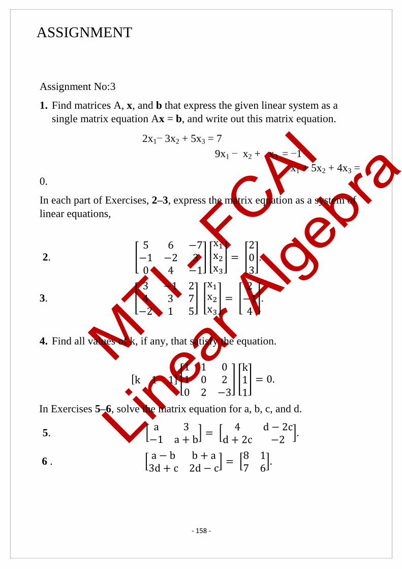
ASSIGNMENT
- 158 -
Assignment No:3
1. Find matrices A, x, and b that express the given linear system as a
single matrix equation Ax = b, and write out this matrix equation.
2x1− 3x2 + 5x3 = 7
9x1 − x2 + x3 = −1
x1 + 5x2 + 4x3 =
0.
In each part of Exercises, 2–3, express the matrix equation as a system of
linear equations,
2. [5 6 −7−1 −2 30 4 −1
] [
x1x2x3] = [
203].
3. [3 −1 24 3 7−2 1 5
] [
x1x2x3] = [
2−14].
4. Find all values of k, if any, that satisfy the equation.
[k 1 1] [1 1 01 0 20 2 −3
] [k11] = 0.
In Exercises 5–6, solve the matrix equation for a, b, c, and d.
5. [a 3−1 a + b
] = [4 d − 2c
d + 2c −2].
6 . [a − b b + a3d + c 2d − c
] = [8 17 6
].
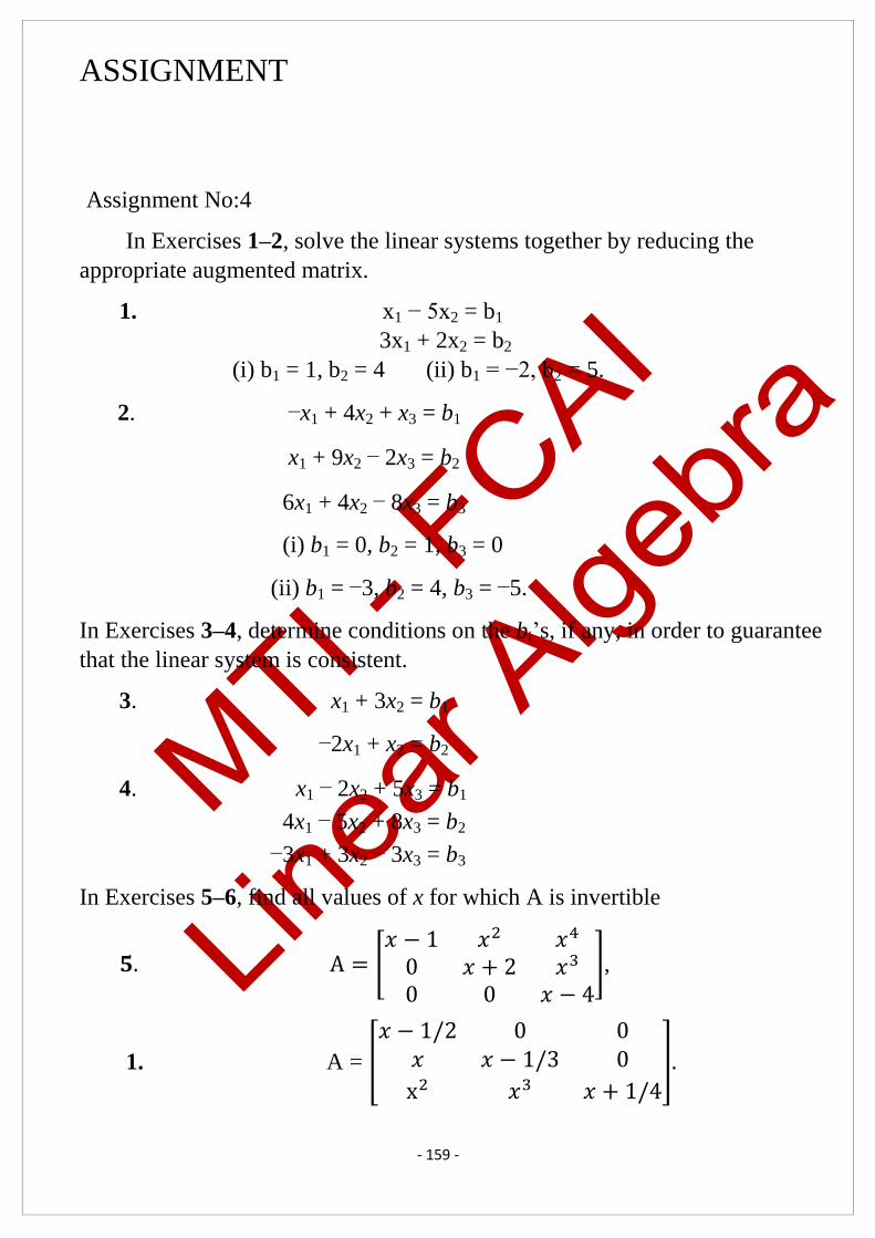
ASSIGNMENT
- 159 -
Assignment No:4
In Exercises 1–2, solve the linear systems together by reducing the
appropriate augmented matrix.
1. x1 − 5x2 = b1
3x1 + 2x2 = b2
(i) b1 = 1, b2 = 4 (ii) b1 = −2, b2 = 5.
2. −x1 + 4x2 + x3 = b1
x1 + 9x2 − 2x3 = b2
6x1 + 4x2 − 8x3 = b3
(i) b1 = 0, b2 = 1, b3 = 0
(ii) b1 = −3, b2 = 4, b3 = −5.
In Exercises 3–4, determine conditions on the bi’s, if any, in order to guarantee
that the linear system is consistent.
3. x1 + 3x2 = b1
−2x1 + x2 = b2
4. x1 − 2x2 + 5x3 = b1
4x1 − 5x2 + 8x3 = b2
−3x1 + 3x2 − 3x3 = b3
In Exercises 5–6, find all values of x for which A is invertible
𝟓. A = [𝑥 − 1 𝑥2 𝑥4
0 𝑥 + 2 𝑥3
0 0 𝑥 − 4
],
1. A = [
𝑥 − 1/2 0 0𝑥 𝑥 − 1/3 0
x2 𝑥3 𝑥 + 1/4].

ASSIGNMENT
- 160 -
Assignment No:5
In Exercises 1–2, find all values of λ for which det(A) = 0.
𝟏. A = [λ − 2 1−5 λ + 4
]. 2. A = [λ − 4 0 00 λ 20 3 λ − 1
].
In Exercises 3–4, evaluate det(A) by a cofactor expansion along a row or
column of your choice.
3. A = [1 𝑘 𝑘2
1 𝑘 𝑘2
1 𝑘 𝑘2]. 4. A = [
𝑘 + 1 𝑘 − 1 72 𝑘 − 3 45 𝑘 + 1 𝑘
].
In each part, show that the value of the determinant is independent of θ.
5. a) |𝑠𝑖𝑛𝜃 𝑐𝑜𝑠𝜃−𝑐𝑜𝑠𝜃 𝑠𝑖𝑛𝜃
|,
b) |𝑠𝑖𝑛𝜃 𝑐𝑜𝑠𝜃 0−𝑐𝑜𝑠𝜃 𝑠𝑖𝑛𝜃 0
𝑠𝑖𝑛𝜃 − 𝑐𝑜𝑠𝜃 𝑠𝑖𝑛𝜃 + 𝑐𝑜𝑠𝜃 1|.
In Exercises 6-7, evaluate the determinant, given that
|
𝑎 𝑏 𝑐𝑑 𝑒 𝑓𝑔 ℎ 𝑖
| = 6
𝟔. |3a 3b 3c−d −e −f4g 4h 4i
|,
2. |a b cd e f2a 2b 2c
|

ASSIGNMENT
- 161 -
Assignment No:6
1. Verify that det (AB) = det (BA).
A = [2 1 0 3 4 0 0 0 2
], B = [1 −1 3 7 1 2 5 0 1
].
2. Find the values of k for which the matrix A is invertible.
A = [1 2 0 𝑘 1 𝑘 0 2 1
].
3. Decide whether the matrix is invertible, and if so, use the adjoint
method to find its inverse.
A = [2 5 5 −1 −1 0 2 4 3
].
4. Solve by Cramer’s rule, where it applies.
x1 –3x2 +x3 = 4 2x1 –x2 = –2 4x1 –3x3 = 0.
5. Find scalars c1, c2, and c3 for which the equation is satisfied
c1(1, −1, 0) + c2(3, 2, 1) + c3(0, 1, 4) = (−1, 1, 19).
6. Let u = (1, −1, 3, 5) and v = (2, 1, 0, −3). Find scalars a and b so that
au + bv = (1, −4, 9, 18).

ASSIGNMENT
- 162 -
Assignment No:7
3. Let v = (−2, 3, 0, 6). Find all scalars k such that ‖kv‖ = 5.
4. Find the Euclidean distance between u and v and the cosine of the
angle between those vectors. State whether that angle is acute, obtuse,
or 90◦.
u = (3, 3, 3), v = (1, 0, 4).
5. Verify that the Cauchy–Schwarz inequality holds.
u = (−3, 1, 0), v = (2, −1, 3).
6. For a vector v = (v1, v2, v3) in R3, let the direction cosines be defined as
cos 𝛼 = 𝑣1
‖𝒗‖, cos 𝛽 =
𝑣2
‖𝒗‖ , cos 𝛾 =
𝑣3
‖𝒗‖.
Show that
𝑐𝑜𝑠2 𝛼 + 𝑐𝑜𝑠2 𝛽 + 𝑐𝑜𝑠2 𝛾 = 1.
7. Let u, v, and w be the vectors in Exercises 1–2. Compute the vector triple
product directly, and check your result by using parts (d) and (e) of theorem
8.1.
u × (v × w).
6. Find the area of the parallelogram determined by the given vectors u and v.
u = (1, −1, 2), v = (0, 3, 1).
7- Find the area of the triangle with the given vertices.
A(2, 0), B(3, 4), C(−1, 2).
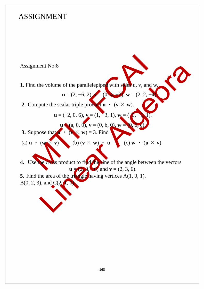
ASSIGNMENT
- 163 -
Assignment No:8
1. Find the volume of the parallelepiped with sides u, v, and w.
u = (2, −6, 2), v = (0, 4, −2), w = (2, 2, −4).
2. Compute the scalar triple product u ・ (v × w).
u = (−2, 0, 6), v = (1, −3, 1), w = (−5, −1, 1).
u = (a, 0, 0), v = (0, b, 0), w = (0, 0, c).
3. Suppose that u ・ (v × w) = 3. Find
(a) u ・ (w × v) (b) (v × w) ・ u (c) w ・ (u × v).
4. Use the cross product to find the sine of the angle between the vectors
u = (2, 3, −6) and v = (2, 3, 6).
5. Find the area of the triangle having vertices A(1, 0, 1),
B(0, 2, 3), and C(2, 1, 0).

ASSIGNMENT
- 164 -

Reference
- 165 -
References:
1- Fundamentals of Linear Algebra by J. S. Chahal, 2019.
2- Linear Algebra and Group Theory for Physicists and Engineers by Yair
Shapira, 2019.
3- Linear Algebra Done Right (3rd edition) by Sheldon Axler, 2019
4- Elementary Linear Algebra (11th
edition) by Howard Anton, and Chris Rorres,
2014.