Linear Algebra and its Applications - UMD Department of ...elman/papers/subsp_iter.pdf · Linear Algebra and its Applications 435 (2011) 601–622 Contents lists available at ScienceDirect

Linear Algebra and its Applications 435 (2011) 601–622

Contents lists available at ScienceDirect

Linear Algebra and its Applications

j ourna l homepage: www.e lsev ie r .com/ loca te / laa

Fast inexact subspace iteration for generalized eigenvalue

problems with spectral transformation�

Fei Xue a, Howard C. Elman b,∗a Applied Mathematics and Scientific Computation Program, Department of Mathematics, University of Maryland,

College Park, MD 20742, USAb Department of Computer Science and Institute for Advanced Computer Studies, University of Maryland,

College Park, MD 20742, USA

A R T I C L E I N F O A B S T R A C T

Submitted by V. Mehrmann

Dedicated to G.W. Stewart on the occasion of

his 70th birthday

Keywords:

Inexact subspace iteration

Tuned preconditioner

Deflation

Subspace recycling

Starting vector

We study inexact subspace iteration for solving generalized non-

Hermitian eigenvalue problems with spectral transformation, with

focus on a few strategies that help accelerate preconditioned

iterative solution of the linear systems of equations arising in

this context. We provide new insights into a special type of pre-

conditioner with “tuning” that has been studied for this algorithm

applied to standard eigenvalue problems. Specifically, we propose

an alternative way to use the tuned preconditioner to achieve

similar performance for generalized problems, and we show that

these performance improvements can also be obtained by solving

an inexpensive least squares problem. In addition, we show that

the cost of iterative solution of the linear systems can be further

reducedbyusingdeflationof convergedSchur vectors, special start-

ing vectors constructed from previously solved linear systems, and

iterative linear solvers with subspace recycling. The effectiveness

of these techniques is demonstrated by numerical experiments.

© 2010 Elsevier Inc. All rights reserved.

�This workwas supported by the U.S. Department of Energy under grant DEFG0204ER25619, and by the U.S. National Science

Foundation under grant CCF0726017.∗ Corresponding author.

E-mail addresses: [email protected] (F. Xue), [email protected] (H. Elman).

0024-3795/$ - see front matter © 2010 Elsevier Inc. All rights reserved.

doi:10.1016/j.laa.2010.06.021

http://www.sciencedirect.com/science/journal/00243795

mailto:[email protected]

mailto:[email protected]

602 F. Xue, H.C. Elman / Linear Algebra and its Applications 435 (2011) 601–622

1. Introduction

Inmany scientific applications, one needs to solve the generalized non-Hermitian eigenvalue prob-

lem Av = λBv for a small group of eigenvalues clustered around a given shift or with largest real parts.

Themost commonly used approach is to employ a spectral transformation tomap these eigenvalues to

extremal ones so that they can be easily captured by eigenvalue algorithms. Themajor difficulty of the

spectral transformation is that a linear system of equations involving a shiftedmatrix A − σBmust be

solved in each (outer) iteration of the eigenvalue algorithm. If the matrices are so large (for example,

those from discretization of three-dimensional partial differential equations) that direct linear solvers

based on factorization are too expensive to apply, we have to use iterative methods (inner iteration)

to solve these linear systems to some prescribed tolerances. Obviously, the effectiveness of the whole

algorithm with “inner–outer” structure depends strongly on that of the inner iteration. In this paper,

we study a few techniques that help accelerate the iterative solution of the linear systems that arise

when inexact subspace iteration is used to solve the generalized non-Hermitian eigenvalue problem

with spectral transformation.

In recent years, great progress has been made in analyzing inexact algorithms, especially inexact

inverse iteration, to compute a simple eigenvalue closest to some shift. Refs. [17,20] establish the

linear convergence of the outer iteration for non-Hermitian problems, assuming that the algorithm

uses a fixed shift and a sequence of decreasing tolerances for the solution of the linear systems. Inexact

Rayleigh quotient iteration for symmetric matrices is studied in [32,26], where the authors explore

how the inexactness of the solution to the linear systems affects the convergence of the outer iteration.

Systematic analysis of this algorithm is given by Spence and his collaborators (see [1–3,12,13]) on the

relation between the inner and the outer iterations, with different formulations of the linear systems,

and variable shifts and tolerances for solving the linear systems. To make the inner iteration converge

more quickly, [31] provides new perspectives on preconditioning by modifying the right hand side of

the preconditioned system. This idea is elaborated on in [1–3] and further refined in [12,13] where a

special type of preconditioner with “tuning” is defined and shown to greatly reduce the inner iteration

counts.

Inexact subspace iteration is a straightforward block extension of inexact inverse iteration with a

fixed shift. Robbé et al. [28] establish linear convergence of the outer iteration of this algorithm for

standard eigenvalue problems and show by the block-GMRES [30] convergence theory that tuning

keeps the block-GMRES iteration counts roughly constant for solving the block linear systems, though

the inner solve is required to be done with increasing accuracy as the outer iteration proceeds. In this

paper, this idea is extended to generalized problems and is improved by a new two-phase algorithm.

Specifically, we show that tuning can be limited to just one step of preconditioned block-GMRES to get

an approximate solution, after which a correction equation can be solved to a fixed relative tolerance

with proper preconditioned block linear solvers where tuning is not needed. We show that the effect

of tuning is to reduce the residual in a special way, and that this effect can be also achieved by other

means, in particular by solving a small least squares problem. Moreover, we show that the two-phase

strategy is closely related to an inverse correction scheme presented in [29,17] and the residual inverse

power method in [34].

The second phase of this algorithm, in addition to using a simplified preconditioning strategy, can

also be simplified in other ways to achieve additional reduction of inner iteration cost. We explore

three techniques to attain the extra speedup:

1. Deflation of converged Schur vectors (see [33]) – Once some Schur vectors have converged, they

are deflated from the block linear systems in subsequent outer iterations, so that the block

size becomes smaller. This approach is independent of the way the block linear systems are

solved.

2. Special starting vector –Wefind that the right hand sides of a few successive correction equations

are often close to being linearly dependent; therefore an appropriate linear combination of the

solutions to previously solved correction equations can be used as a good starting vector for

solving the current one.

F. Xue, H.C. Elman / Linear Algebra and its Applications 435 (2011) 601–622 603

3. Subspace recycling – Linear solvers with recycled subspaces (see [27]) can be used to solve the

sequence of correction equations, so that the search space for each solve does not need to be

built from scratch. In addition, if the same preconditioner is used for all correction equations, the

recycled subspaces available from solving one equation can be used directly for the next without

being transformed by additional preconditioned matrix–vector products.

We discuss the effectiveness of these ideas and show by numerical experiments that they generally

result in significant savings in the number of preconditioned matrix–vector products performed in

inner iterations.

An outline of the paper is as follows. In Section 2, we describe the inexact subspace iteration

for generalized non-Hermitian eigenvalue problems, restate some preliminary results taken from

[28] about block decomposition of matrices, and discuss a new tool for measuring closeness of two

subspaces. In Section 3,we briefly discuss the behavior of unpreconditioned andpreconditioned block-

GMRES without tuning for solving the block linear systems arising in inexact subspace iteration,

and present new insights into tuning that lead to our two-phase strategy to solve the block linear

systems. In Section 4, we discuss deflation of converged Schur vectors, special starting vector and

linear solvers with recycled subspaces and the effectiveness of the combined use of these techniques

for solving the block systems. Section 5 includes a series of numerical experiments to show the

performance of our algorithm for problems from Matrix Market [22] and those arising from linear

stability analysis of models of two-dimensional incompressible flows. We finally draw conclusions in

Section 6.

2. Inexact subspace iteration and preliminary results

In this section, we review inexact subspace iteration for the generalized non-Hermitian eigenvalue

problem Av = λBv (A, B ∈ Cn×n)with spectral transformation, block Schur and eigen-decomposition

of matrices, and metrics that measure the error of the current approximate invariant

subspace.

2.1. Spectral transformation and inexact subspace iteration

To better understand the algorithm, we start with the definition of the shift-invert and the gener-

alized Cayley transformation (see [23]) as follows:

Av = λBv ⇔ (A − σB)−1Bv = 1

λ − σv (shift�invert) (2.1)

Av = λBv ⇔ (A − σ1B)−1(A − σ2B)v = λ − σ2

λ − σ1

v (generalized Cayley)

The shift-invert transformation maps eigenvalues closest to σ to dominant eigenvalues of A = (A −σB)−1B; thegeneralizedCayley transformationmapseigenvalues to the rightof the line�(λ) = σ1+σ2

2

to eigenvalues ofA = (A − σ1B)−1(A − σ2B) outside the unit circle, and those to the left of this line to

ones inside the unit circle (assuming that σ1 > σ2). The eigenvalues of A with largest magnitude can

be easily found by iterative eigenvalue algorithms. Once the eigenvalues of the transformed problem

are found, they are transformed back to those of the original problem. Note that the eigenvectors do

not change with the transformation.

Without loss of generality, we consider using A = A−1B for inexact subspace iteration to compute

k eigenvalues of Av = λBv with smallest magnitude (i.e., k dominant eigenvalues of A = A−1B). This

notation covers both types of operators in (2.1) with arbitrary shifts. For example, one can let A =A − σ1B and B = A − σ2B, so that the generalized Cayley operator is A = A−1B. The algorithm is as

follows:


Algorithm 1. Inexact subspace iteration with A = A−1B.

Given δ � 0 and X(0) ∈ Cn×p with X(0)∗X(0) = I (k � p)For i = 0, 1, . . . , until k Schur vectors converge

1. Compute the error e(i) = sin∠(AX (i), BX (i))

2. Solve AY (i) = BX(i) inexactly such that the relative residual norm‖BX(i)−AY (i)‖

‖BX(i)‖ � δe(i)

3. Perform the Schur–Rayleigh–Ritz procedure to get X(i+1) with orthonormal columns

from Y (i) and test for convergence

End For

In Step 1, X (i) is the space spanned by the current outer iterate X(i). The error of X(i) is defined as

the sine of the largest principal angle between AX (i) and BX (i). It decreases to zero as X(i) converges

to an invariant subspace of the matrix pencil (A, B). This error can be computed by MATLAB’s function

subspace based on singular value decomposition (see Algorithm 12.4.3 of [16]), and will be discussed

in detail in Proposition 2.2.

The Schur–Rayleigh–Ritz (SRR) procedure (seeChapter 6.1 of [33]) in Step3will be applied todeflate

converged Schur vectors. The procedure and its use for deflationwill be explained in detail in Section 4.

Themost computationally expensive part of the algorithm is Step 2, which requires an inexact solve of

the block linear system AY (i) = BX(i). Themajor concern of this paper is to reduce the cost of this solve.

2.2. Block eigen-decomposition

To briefly review the basic notations and description of the generalized eigenvalue problem, we re-

state some results from [28] onblock eigen-decompositionofmatrices and study anew tool tomeasure

the error of X(i) for generalized problems. To simplify our exposition, we assume that B is nonsingular.

This assumption is valid for problems arising in a variety of applications. In addition, though B is only

positive semi-definite in linear stability analysis of incompressible flows, one can instead solve some

related eigenvalue problems with nonsingular B that share the same finite eigenvalues as the original

problem; see [4] for details.

As B is nonsingular, we assume that the eigenvalues of B−1A are ordered so that

0 < |λ1| � |λ2| � . . . � |λp| < |λp+1| � . . . � |λn|.The Schur decomposition of B−1A can be written in block form as

B−1A =[V1, V

⊥1

] [T11 T120 T22

] [V1, V

⊥1

]∗, (2.2)

where[V1, V

⊥1

]is a unitary matrix with V1 ∈ Cn×p and V⊥

1 ∈ Cn×(n−p), T11 ∈ Cp×p and T22 ∈C(n−p)×(n−p) are upper triangular, λ(T11) = {λ1, . . . , λp} and λ(T22) = {λp+1, . . . , λn}. Since T11 and

T22 have disjoint spectra, there is a unique solution Q ∈ Cp×(n−p) to the Sylvester equation QT22 −T11Q = T12 (see Section 1.5, Chapter 1 of [33]). Then B−1A can be transformed to block-diagonal form

as follows:

B−1A =[V1, V

⊥1

] [ I Q

0 I

] [T11 0

0 T22

] [I −Q

0 I

] [V1, V

⊥1

]∗=

[V1, (V1Q + V⊥

1 )] [T11 0

0 T22

] [(V1 − V⊥

1 Q∗), V⊥1

]∗=

[V1, (V1Q + V⊥

1 )Q−1D

] [T11 0

0 QDT22Q−1D

] [(V1 − V⊥

1 Q∗), V⊥1 QD

]∗= [V1, V2]

[K 0

0 M

][W1, W2]

∗ = [V1, V2]

[K 0

0 M

][V1, V2]

−1 , (2.3)


where QD = (I + Q∗Q)1/2, V2 = (V1Q + V⊥1 )Q−1

D with orthonormal columns, K = T11, M = QDT22

Q−1D with the same spectrum as T22, W1 = V1 − V⊥

1 Q∗ and W2 = V⊥1 QD such that [W1, W2]

∗ =[V1, V2]

−1. From the last expression of (2.3), we have

AV1 = BV1K, and AV2 = BV2M. (2.4)

Recall that we want to compute V1 and corresponding eigenvalues (the spectrum of K) by inexact

subspace iteration.

2.3. Tools to measure the error

The basic tool to measure the deviation of X (i) = span{X(i)} from V1 = span{V1} is the sine of the

largest principal angle between X (i) and V1 defined as (see [28] and references therein)

sin(X (i), V1)=‖(V⊥1 )∗X(i)‖ = ‖X(i)(X(i))∗ − V1V

∗1 ‖

= minZ∈Cp×p

‖X(i) − V1Z‖ = minZ∈Cp×p

‖V1 − X(i)Z‖. (2.5)

This definition depends on the fact that both X(i) and V1 have orthonormal columns.

We assume that X(i) has the following decomposition

X(i) = V1C(i) + V2S

(i) with ‖S(i)‖ < 1, (2.6)

where C(i) = W∗1 X

(i) ∈ Cp×p, S(i) = W∗2 X

(i) ∈ C(n−p)×p. Intuitively, ‖S(i)‖ → 0 as X (i) → V1. Prop-

erties of C(i) and the equivalence of several metrics are given in the following proposition.

Proposition2.1 (Proposition 2.1 in [28]). Suppose X(i) is decomposed as in (2.6). Let s(i) = ‖S(i)(C(i))−1‖and t(i) = s(i)‖C(i)‖. Then

(1) C(i) is nonsingular and thus t(i) is well-defined. The singular values of C(i) satisfy

0 < 1 − ‖S(i)‖ � σk(C(i)) � 1 + ‖S(i)‖, k = 1, 2, . . . , p (2.7)

and C(i) = U(i) + ϒ(i), where U(i) is unitary and ‖ϒ(i)‖ � ‖S(i)‖ < 1.

(2a) sin(X (i), V1) � ‖S(i)‖ � s(i) �(

1+‖S(i)‖1−‖S(i)‖

)‖S(i)‖.

(2b) sin(X (i), V1) � t(i) � ‖S(i)‖1−‖S(i)‖ .

(2c) ‖S(i)‖ �√1 + ‖Q‖2 sin(X (i), V1).

The proposition states that as X (i) → V1, C(i) gradually approximates a unitary matrix, and

sin(X (i), V1), ‖S(i)‖, s(i) and t(i) are essentially equivalent measures of the error. These quantities

are not computable since V1 is not available. However, the computable quantity sin(AX (i), BX (i)) in

Step 1 of Algorithm 1 is equivalent to ‖S(i)‖, as the following proposition shows.

Proposition 2.2. Let X(i) be decomposed as in (2.6). Then

c1‖S(i)‖ � sin(AX (i), BX (i)) � c2‖S(i)‖, (2.8)

where c1 and c2 are constants independent of the progress of subspace iteration.


Proof. We first show that as X (i) → V1, AX (i) ≈ BX (i). In fact, from (2.4) and (2.6) we have

BX(i) = BV1C(i) + BV2S

(i) = AV1K−1C(i) + AV2M

−1S(i)

= A(X(i) − V2S(i))(C(i))−1K−1C(i) + AV2M

−1S(i)

= AX(i)(C(i))−1K−1C(i) − AV2

(S(i)(C(i))−1K−1C(i) − M−1S(i)

). (2.9)

Roughly speaking,AX(i) and BX(i) can be transformed to each other by postmultiplying (C(i))−1K−1C(i)

or its inverse, with a small error proportional to ‖S(i)‖.Let D

(i)A = (X(i)∗A∗AX(i))−1/2, D

(i)B = (X(i)∗B∗BX(i))−1/2 ∈ Cp×p, so that both AX(i)D

(i)A and

BX(i)D(i)B have orthonormal columns. Then by (2.5)

sin∠(AX (i), BX (i))= minZ∈Cp×p

‖AX(i)D(i)A − BX(i)D

(i)B Z‖

�∥∥∥AX(i)D

(i)A − BX(i)D

(i)B

((D

(i)B )−1(C(i))−1KC(i)D

(i)A

)∥∥∥=∥∥∥(AX(i) − BX(i)(C(i))−1KC(i)

)D

(i)A

∥∥∥=∥∥∥BV2

(MS(i) − S(i)(C(i))−1KC(i)

)D

(i)A

∥∥∥ (see (2.9) and (2.4))

�‖BV2‖‖D(i)A ‖‖Si‖‖S(i)‖, (2.10)

where Si is the Sylvester operator G → Si(G) : MG − G(C(i))−1KC(i). Note that as i increases, ‖Si‖ →‖S‖ where S : G → S(G) = MG − GK . In fact,

‖Si‖ = supG

‖MG − G(C(i))−1KC(i)‖‖G‖ (G ∈ C(n−p)×p)

= supG

∥∥∥(M (G(C(i))−1

)−(G(C(i))−1

)K)C(i)

∥∥∥‖(G(C(i))−1

)C(i)‖ , (2.11)

and therefore

supG

‖MG − GK‖‖G‖κ(C(i))

� ‖Si‖ � supG

‖MG − GK‖κ(C(i))

‖G‖ (G ∈ C(n−p)×p)

or ‖S‖/κ(C(i)) � ‖Si‖ � ‖S‖κ(C(i)). (2.12)

As 1� κ(C(i)) � 1+‖S(i)‖1−‖S(i)‖ (Proposition 2.1, 2a) and ‖S(i)‖ → 0, ‖Si‖ → ‖S‖ follows. Also, note that the

extremal singular values ofD(i)A are bounded by those of (A∗A)−1/2 (equivalently, those of A−1), so that

in particular ‖D(i)A ‖ is bounded above by a constant independent of i. The upper bound in (2.8) is thus

established.

To study the lower bound, we have

sin∠(AX (i), BX (i))= minZ∈Cp×p

‖AX(i)D(i)A − BX(i)D

(i)B Z‖

= minZ∈Cp×p

∥∥∥B (B−1AX(i) − X(i)D(i)B Z(D

(i)A )−1

)D

(i)A

∥∥∥� min

Z∈Cp×p‖B−1AX(i) − X(i)Z‖σmin(B)σmin(D

(i)A ). (2.13)


Let σ (i) = σmin(B)σmin(D(i)A ) = σmin(B)‖X(i)∗A∗AX(i)‖−1/2. Again using the boundedness of the sin-

gular values of D(i)A , it follows that σ (i) is bounded below by a constant independent of i. Since the

minimizer Z in the inequality (2.13) is K(i) = X(i)∗B−1AX(i) (see Chapter 4, Theorem 2.6 of [33]), we

have

sin∠(AX (i), BX (i)) � σ (i)‖B−1AX(i) − X(i)K(i)‖� σ (i)‖(V⊥

1 )∗(B−1AX(i) − X(i)K(i))‖ ( ‖V⊥1 ‖ = 1 )

= σ (i)‖T22(V⊥1 )∗X(i) − (V⊥

1 )∗X(i)K(i)‖ ( (V⊥1 )∗B−1A = T22(V

⊥1 )∗; see (2.2))

� σ (i)sep(T22, K(i))‖(V⊥

1 )∗X(i)‖ = σ (i)sep(T22, K(i)) sin∠(V1,X (i))

� σ (i)sep(T22, K(i))(1 + ‖Q‖2)−1/2‖S(i)‖. (Proposition 2.1(2c)) (2.14)

Moreover, as X (i) → V1, K(i) = X(i)∗B−1AX(i) → K up to a unitary transformation, and hence

sep(T22, K(i)) → sep(T22, K) (see Chapter 4, Theorem 2.11 in [33]). This concludes the proof. �

Remark 2.1. In [28] the authors use ‖AX(i) − X(i)(X(i)∗AX(i))‖ to estimate the error ofX(i) for standard

eigenvalue problems, and show that this quantity is essentially equivalent to ‖S(i)‖. The p × pmatrix

X(i)∗AX(i) is called the (block) Rayleigh quotient of A (see Chapter 4, Definition 2.7 of [33]). For the

generalized eigenvalue problem, we have not seen an analogous quantity in the literature. However,

Proposition 2.2 shows that sin∠(AX (i), BX (i)) is a convenient error estimate.

3. Convergence analysis of inexact subspace iteration

We first demonstrate the linear convergence of the outer iteration of Algorithm 1, which follows

from Theorem 3.1 in [28]. In fact, replacing A−1 by A−1B in the proof therein, we have

t(i+1) � ‖K‖‖M−1‖ t(i) + ‖W∗2 B

−1‖ ‖(C(i))−1‖ ‖R(i)‖1 − ‖W∗

1 B−1‖ ‖(C(i))−1‖ ‖R(i)‖ , (3.1)

where ‖(C(i))−1‖ = 1/σmin(C(i)) → 1, and

‖R(i)‖=‖BX(i) − AY (i)‖ � δ‖BX(i)‖ sin∠(AX (i), BX (i))

�δC2‖BX(i)‖√1 + ‖Q‖2t(i). (see Proposition 2.1) (3.2)

Thus X (i) → V1 linearly for ‖K‖‖M−1‖ < 1 and small enough δ.In this section, we investigate the convergence of unpreconditioned and preconditioned block-

GMRES without tuning for solving AY (i) = BX(i) to the prescribed tolerance, and provide new per-

spectives on tuning that lead to a new two-phase strategy for solving this block system.

3.1. Unpreconditioned and preconditioned block-GMRES with no tuning

The block linear systems AY (i) = X(i) arising in inexact subspace iteration for standard eigenvalue

problems are solved to increasing accuracy as the outer iteration progresses. It is shown in [28] that

when unpreconditioned block-GMRES is used for these systems, iteration counts remain roughly con-

stant during the course of this computation, but for preconditioned block-GMRES without tuning, the

number of iterations increases with the outer iteration. The reason is that the right hand side X(i) is

an approximate invariant subspace of the system matrix A, whereas with preconditioning, there is

no reason for X(i) to bear such a relation to the preconditioned system matrix AP−1 (assuming right

preconditioning is used).


For generalized eigenvalue problems, however, both the unpreconditioned and preconditioned

block-GMRES iteration counts increase progressively. To see this point, we study the block spectral

decomposition of the system matrix and right hand side and review the block-GMRES convergence

theory. We present the analysis of the unpreconditioned solve; the results apply verbatim to the

preconditioned solve.

We first review a generic convergence result of block-GMRES given in [28]. Let G be a matrix of

order n where the p smallest eigenvalues are separated from its other n − p eigenvalues. As in (2.3),

we can block diagonalize G as

G = [VG1, VG2]

[KG 0

0 MG

][VG1, VG2]

−1 , (3.3)

where VG1 ∈ Cn×p and VG2 ∈ Cn×(n−p) have orthonormal columns, λ(KG) are the p smallest eigen-

values of G, and λ(MG) are the other eigenvalues of G. Recall the definitions of the numerical range

W(MG) ={z∗MGzz∗z : z ∈ Cn−p, z /= 0

}and the ε-pseudospectrumλε(MG) = {λ ∈ C : σmin(λI − MG)

� ε}. The role of the right hand side in the convergence of block-GMRES is described in the following

lemma, which follows immediately from Theorem 3.7 of [28].

Lemma 3.1. Assume the numerical range W(MG) or the ε-pseudospectrum λε(MG) is contained in a

convex closed bounded set E in the complex plane with 0 /∈ E. Suppose block-GMRES is used to solve

GY = Z where Z ∈ Cn×p can be decomposed as Z = VG1CG + VG2SG with VG1 and VG2 given in (3.3).

Here SG ∈ C(n−p)×p, and we assume CG ∈ Cp×p is nonsingular. Let Yk be the approximate solution of

GY = Z obtained in the k-th block-GMRES iteration with Y0 = 0. If

k � 1 + Ca

(Cb + log

‖CG‖‖SGC−1G ‖

‖Z‖τ), (3.4)

then‖Z−GYk‖‖Z‖ � τ. Here Ca and Cb are constants that depend on the spectrum of G.

Remark 3.1. For details about Ca and Cb, see [28,18,11]. These details have minimal impact on our

subsequent analysis.

Remark 3.2. This generic convergence result can be applied to any specific block linear systems with

or without preconditioning. For example, to study the behavior of unpreconditioned block-GMRES for

solvingAY (i) = BX(i), letG = A in (3.3) and Lemma3.1, and decompose relevant sets of columnvectors

in terms of VA1 and VA2.

In the following, we will assume that for nontrivial B (B /= I), there is no pathological or trivial

connectionbetween thedecompositionof (3.3) for the caseG = Aand that ofB−1A in (2.3). Specifically,

we assume there exist a nonsingular C1 ∈ Cp×p and a full rank S1 ∈ C(n−p)×p such that

V1 = VA1C1 + VA2S1. (3.5)

This assumption is generally far from stringent in practice. Similarly, let the decomposition of V2 be

V2 = VA1C2 + VA2S2 with C2 ∈ Cp×(n−p) and S2 ∈ C(n−p)×(n−p).

Lemma3.1 and theassumptions above lead to the following theorem,whichgivesqualitative insight

into the behavior of block-GMRES for solving AY (i) = BX(i).

Theorem 3.2. Assume that unpreconditioned block-GMRES is used to solve the linear system AY (i) =BX(i) to the prescribed tolerance in Step 2 of Algorithm 1. If the assumption (3.5) holds, and X (i) → V1

linearly, then the lower bound on block-GMRES iterations from Lemma 3.1 increases as the outer iteration

proceeds.


Proof. With (2.4), (2.6), (3.3) and (3.5), we have

BX(i) = BV1C(i) + BV2S

(i) = AV1K−1C(i) + AV2M

−1S(i)

= A(VA1C1 + VA2S1)K−1C(i) + A(VA1C2 + VA2S2)M

−1S(i)

= (VA1KAC1 + VA2MAS1)K−1C(i) + (VA1KAC2 + VA2MAS2)M

−1S(i)

= VA1KA(C1K−1C(i) + C2M

−1S(i)) + VA2MA(S1K−1C(i) + S2M

−1S(i))

= VA1C(i)A + VA2S

(i)A . (3.6)

Since ‖S(i)‖ → 0 and σk(C(i)) → 1(k = 1, 2, . . . , p) (see Proposition 2.1(1)), we have ‖C(i)

A ‖ →‖KAC1K

−1‖ and ‖S(i)A (C

(i)A )−1‖ → ‖MAS1C

−11 K

−1A ‖, both of which are nonzero under our assumption

(3.5).

From Step 2 of Algorithm 1 and (2.10), the relative tolerance for AY (i) = BX(i) is τ = δ sin(AX (i),

BX (i)) � δ‖BV2‖‖D(i)A ‖‖Si‖‖S(i)‖ → 0. Then from (3.4) and (3.6), the lower bound of the unprecondi-

tioned block-GMRES iteration counts needed for solving AY (i) = BX(i) to the prescribed tolerance is

k(i) � 1 + Ca

⎛⎝Cb + log‖C(i)

A ‖‖S(i)A (C

(i)A )−1‖

δ‖BX(i)‖‖BV2‖‖D(i)A ‖‖Si‖‖S(i)‖

⎞⎠ . (3.7)

Note that‖BX(i)‖ → ‖BV1‖,‖D(i)A ‖ → ‖(V1A

∗AV1)−1/2‖ and‖Si‖ → ‖S‖ (see the proof of Propo-

sition 2.2). Therefore all terms in the argument of the logarithm operator approach some nonzero

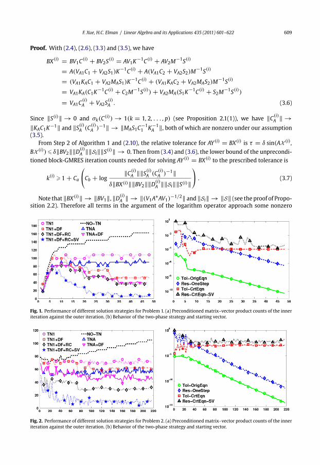
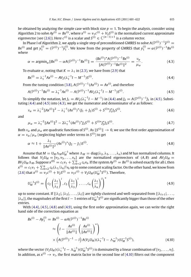
Fig. 1. Performance of different solution strategies for Problem 1. (a) Preconditioned matrix–vector product counts of the inner

iteration against the outer iteration. (b) Behavior of the two-phase strategy and starting vector.

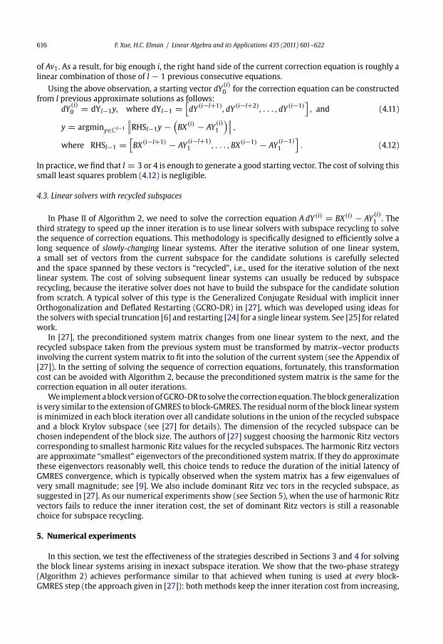
Fig. 2. Performance of different solution strategies for Problem 2. (a) Preconditionedmatrix–vector product counts of the inner

iteration against the outer iteration. (b) Behavior of the two-phase strategy and starting vector.


limit except ‖S(i)‖ → 0, and hence the expression on the right in (3.7) increases as the outer iteration

proceeds. �

Remark 3.3. This result only shows that a lower bound on k(i) increases; it does not establish that

there will be growth in actual iteration counts. However, numerical experiments described in [28] and

Section 5 (see Figs. 1 and 2) show that this result is indicative of performance. The fact that the bound

progressively increases depends on the assumption of (3.5) that V1 has “regular” components of VA1

and VA2. This assumption guarantees that BX (i) does not approximate the invariant subspace VA1 of A.

The proof also applies word for word to the preconditioned solve without tuning: one only needs to

replace (3.3) by the decomposition of the preconditioned systemmatrix AP−1 andwrite BX(i) in terms

of the invariant subspace of AP−1.

3.2. Preconditioned block-GMRES with tuning

To accelerate the iterative solution of the block linear system arising in inexact subspace iteration,

[28] proposes and analyzes a new type of preconditioner with tuning. Tuning constructs a special low-

rank update of the existing preconditioner, so that the right hand side of the preconditioned system is

an approximate eigenvector or invariant subspace of the preconditioned system matrix with tuning.

Specifically, the tuned preconditioner is

P(i) = P + (AX(i) − PX(i))X(i)∗, (3.8)

fromwhich follow P(i)X(i) = AX(i) and A(P(i))−1(AX(i)) = AX(i). In other words, AX (i) is an invariant

subspace of A(P(i))−1 with eigenvalue 1. Intuitively, as X (i) → V1, we have X (i) ≈ AX (i) for the

standard eigenvalue problem, or BX (i) ≈ AX (i) for the generalized problem. Therefore, the right hand

side of A(P(i))−1Y (i) = X(i) or A(P(i))−1Y (i) = BX(i) (with Y (i) = (P(i))−1Y (i)) spans an approximate

invariant subspace of A(P(i))−1. The difficulty of block-GMRESwithout tuning discussed in Section 3.1

is thus resolved, and the block-GMRES iteration counts with tuning do not increase with the progress

of the outer iteration (see Theorem 4.5 of [28]).

The matrix–vector product involving (P(i))−1 is built from that for P−1 using the Sherman–

Morrison–Woodbury formula as follows:

(P(i))−1 =(I − (P−1AX(i) − X(i))

(X(i)∗P−1AX(i)

)−1X(i)∗

)P−1. (3.9)

Note that P−1AX(i) − X(i) and X(i)∗P−1AX(i) can be computed before the block-GMRES iteration. In

each block-GMRES step, (P(i))−1 requires an additional p2 inner products of vectors of length n, a

dense matrix–matrix division of size p × p, and a multiplication of a dense matrix of size n × p with

a p × pmatrix. This extra cost is relatively small in general, but it is not free.

We now provide a new two-phase algorithm for solving AY (i) = BX(i), which essentially eliminates

the overhead of tuning but keeps the block-GMRES iteration counts from progressively increasing.

The strategy provides some new perspectives on the use of tuning. In addition, we will discuss some

connections between this algorithm and the methods in [29,17,34].

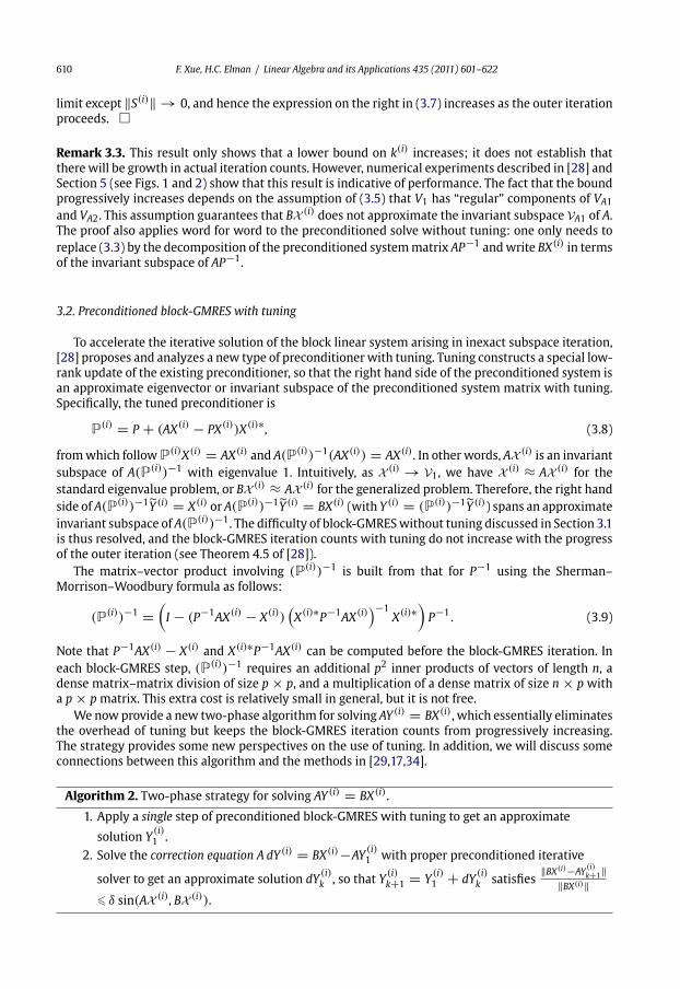
Algorithm 2. Two-phase strategy for solving AY (i) = BX(i).

1. Apply a single step of preconditioned block-GMRES with tuning to get an approximate

solution Y(i)1 .

2. Solve the correction equation A dY (i) = BX(i)−AY(i)1 with proper preconditioned iterative

solver to get an approximate solution dY(i)k , so that Y

(i)k+1 = Y

(i)1 + dY

(i)k satisfies

‖BX(i)−AY(i)k+1‖

‖BX(i)‖� δ sin(AX (i), BX (i)).


Note in particular that tuning need not be used to solve the correction equation, and thus we can

work with a fixed preconditioned system matrix for the correction equation in all outer iterations.

Obviously, Phase II can be equivalently stated as follows: solve AY (i) = BX(i) with proper precon-

ditioned iterative solver and starting vector Y(i)1 from Phase I. The phrasing in Algorithm 2 is intended

to illuminate the connection between this strategy and the methods in [29,17,34].

The analysis of Algorithm2 is given in the followingmain theorem. For this,wemake some assump-

tions concerning the right hand side of the correction equation analogous to the assumption made for

(3.5): with

BX(i) − AY(i)1 = VA1C

(i)ceq + VA2S

(i)ceq, (3.10)

where VA1 and VA2 have orthonormal columns,we assume that ‖S(i)ceq(C

−1ceq )

(i)‖ = O(1), and that ‖Cceq‖is proportional to ‖BX(i) − AY

(i)1 ‖. This implies that the term

‖C(i)ceq‖ ‖S(i)

ceq(C−1ceq )(i)‖

‖BX(i)−AY(i)1 ‖ , which appears in (3.4),

does not depend on i. We have no proof of these assumptions, but they are consistent with all our

numerical experience. In the subsequent derivation, let ej ∈ Rp be a standard unit basis vector with 1

in entry j and zero in other entries.

Theorem 3.3. Suppose the two-phase strategy (Algorithm 2) is used to solve AY (i) = BX(i). Then Y(i)1 =

X(i)(C(i))−1K−1C(i)F + (i) where F = [f1, . . . , fp] with fj = argminf∈Cp‖BX(i)ej − A(P(i))−1BX(i)f‖and ‖(i)‖ = O(‖S(i)‖). In addition, the residual norm ‖BX(i) − AY

(i)1 ‖ = O(‖S(i)‖). Thus, if block-

GMRES is used to solve the correction equation, the inner iteration countswill not increasewith the progress

of the outer iteration.

Proof. The approximate solution to A(P(i))−1Y = BX(i) in the k-th block-GMRES iteration starting

with zero starting vector is

Y(i)k ∈ span{BX(i), A(P(i))−1BX(i), . . . ,

(A(P(i))−1

)k−1BX(i)}. (3.11)

It follows from (2.9) and (P(i))−1AX(i) = X(i) that

Y(i)1 = (P(i))−1Y

(i)1 = (P(i))−1BX(i)F

= (P(i))−1(AX(i)(C(i))−1K−1C(i) − AV2

(S(i)(C(i))−1K−1C(i) − M−1S(i)

))F

= X(i)(C(i))−1K−1C(i)F + (P(i))−1AV2

(M−1S(i) − S(i)(C(i))−1K−1C(i)

)F

= X(i)(C(i))−1K−1C(i)F + (i), (3.12)

where the jth column of F ∈ Cp×p minimizes ‖BX(i)ej − A(P(i))−1BX(i)f‖, i.e., the residual norm of

the jth individual system (property of block-GMRES), and

‖(i)‖ � ‖(P(i))−1AV2‖‖F‖‖S i‖‖S(i)‖, (3.13)

where theSylvesteroperatorS i : G → S i(G) = M−1G − G(C(i))−1K−1C(i). Using the samederivation

as in the proof of Proposition 2.2, we can show ‖S i‖ → ‖S‖, where S : G → S(G) = M−1G − GK−1.

In addition, since X (i) → V1 in (3.8), it follows that P(i) → P ≡ P + (AV1 − PV1)V∗1 . Thus ‖(i)‖ =

O(‖S(i)‖) is established.We now investigate the residual norm ‖BX(i) − AY

(i)1 ‖ of the linear system after Phase I of

Algorithm 2. Recall the property of tuning that(I − A(P(i))−1

)AX(i) = 0, and the property of block-

GMRES that the approximate solution Y(i)1 ∈ span{BX(i)}. As block-GMRES minimizes the residual

norm of each individual linear system of the block system, the j-th column of the block residual is


∥∥∥(BX(i) − A(P(i))−1Y

(i)1

)ej

∥∥∥ = minf∈Cp

‖BX(i)ej − A(P(i))−1(BX(i)f )‖

�∥∥∥(I − A(P(i)

)−1)BX(i)ej

∥∥∥�∥∥∥(I − A(P(i)

)−1)BX(i)

∥∥∥=

∥∥∥(I − A(P(i))−1

)AV2

(S(i)(C(i))−1K−1C(i) − M−1S(i)

)∥∥∥ (see (2.9))

�∥∥∥(I − A(P(i)

)−1)AV2

∥∥∥ ‖S i‖‖S(i)‖ = O(‖S(i)‖), (3.14)

from which follows

‖BX(i) − AY(i)1 ‖ �

p∑j=1

∥∥∥(BX(i) − A(P(i))−1Y(i)1

)ej

∥∥∥ = O(‖S(i)‖). (3.15)

Finally in Phase II of Algorithm 2, Y(i)k+1 = Y

(i)1 + dY

(i)k , where dY

(i)k is an approximate solution of

the correction equation A dY (i) = BX(i) − AY(i)1 . The stopping criterion requires that

‖BX(i)−AY(i)k+1‖

‖BX(i)‖ = ‖BX(i) − A(Y(i)1 + dY

(i)k )‖

‖BX(i)‖= ‖(BX(i) − AY

(i)1 ) − A dY

(i)k ‖

‖BX(i) − AY(i)1 ‖

‖BX(i) − AY(i)1 ‖

‖BX(i)‖ � δ sin∠(AX (i), BX (i)). (3.16)

Note that‖(BX(i)−AY

(i)1 )−A dY

(i)k ‖

‖BX(i)−AY(i)1 ‖ is the relative residual norm of the correction equation for dY

(i)k , and

‖BX(i)−AY(i)1 ‖

‖BX(i)‖ is the relative residual norm of the original equation for Y(i)1 . It follows that the prescribed

stopping criterion of the inner iteration is satisfied if‖(BX(i)−AY

(i)1 )−A dY

(i)k ‖

‖BX(i)−AY(i)1 ‖ is bounded above by

δ‖BX(i)‖ sin(AX (i), BX (i))

‖BX(i) − AY(i)1 ‖

�δ‖BX(i)‖σ (i)sep(T22, K

(i))∥∥∥(I − A(P(i))−1)AV2

∥∥∥ ‖S i‖√1 + ‖Q‖2

≡ ρ(i), (3.17)

where we apply the lower bound of sin(AX (i), BX (i)) in (2.14) and the upper bound of ‖BX(i) − AY(i)1 ‖

in (3.15).

To study ρ(i), recall from the end of the proof of Proposition 2.2 that σ (i) = σmin(B)‖X(i)∗A∗AX(i)‖−1/2 → σmin(B)‖V∗

1 A∗AV1‖−1/2 > 0, and sep(T22, K

(i)) → sep(T22, K) > 0. In addition,∥∥∥(I − A(P(i))−1)AV2

∥∥∥ →∥∥∥(I − AP−1

)AV2

∥∥∥ and ‖S i‖ → ‖S‖. This means ρ(i), a lower bound of

the relative tolerance for the correction equation, can be fixed independent of i. It then follows from

Lemma 3.1 and our assumption concerning the decomposition (3.10) of BX(i) − AY(i)1 that if block-

GMRES is used to solve the correction equation, the inner iteration counts do not increase with the

progress of the outer iteration. �

3.3. A general strategy for the phase I computation

It can be seen from Theorem 3.3 that the key to the success of the two-phase strategy is that in

the first phase, an approximate solution Y(i)1 is obtainedwhose block residual norm ‖BX(i) − AY

(i)1 ‖ =

O(‖S(i)‖). It is shown in Section 3.2 that such a Y(i)1 can be constructed inexpensively from a single

step of block-GMRES with tuning applied to AY (i) = BX(i). In fact, a valid Y(i)1 can also be constructed

in other ways, in particular, by solving a set of least squares problems

minf∈Cp

‖BX(i)ej − AX(i)fj‖ 1� j � p. (3.18)


This is easily done using the QR factorization of AX(i). The solution fj satisfies

‖BX(i)ej − AX(i)fj‖ = minf∈Cp

‖BX(i)ej − AX(i)f‖� ‖BX(i)ej − AX(i)(C(i))−1K−1C(i)ej‖=

∥∥∥AV2

(S(i)(C(i))−1K−1C(i) − M−1S(i)

)ej

∥∥∥ (see (2.9))

� ‖AV2‖‖S i‖‖S(i)‖ = O(‖S(i)‖). (3.19)

Thus, with Y(i)1 = X(i)[f1, . . . , fp], it follows immediately that

‖BX(i) − AY(i)1 ‖ �

p∑j=1

‖BX(i)ej − AX(i)fj‖ �O(‖S(i)‖), (3.20)

so that the conclusion of Theorem 3.3 is also valid for this choice of Y(i)1 .

This discussion reveals a connection between the two-phase strategy and the inverse correction

method [29,17] and the residual inverse powermethod [34], where the authors independently present

essentially the samekey idea for inexact inverse iteration. For example [34], constructs x(i+1) by adding

a small correction z(i) to x(i). Here, z(i) is the solution of Az = μx(i) − Ax(i), whereμ = x(i)∗Ax(i) is the

Rayleigh quotient, and μx(i) − Ax(i) is the current eigenvalue residual vector that satisfies ‖μx(i) −Ax(i)‖ = minα∈C ‖αx(i) − Ax(i)‖. In Algorithm2,we compute Y

(i)k+1 by adding dY

(i)k to Y

(i)1 , where dY

(i)k

is an approximate solution of A dY (i) = BX(i) − AY(i)1 . Here Y

(i)1 satisfies span{Y (i)

1 } ≈ span{X(i)} (see(3.12)), and ‖BX(i) − AY

(i)1 ‖ is minimized by a single block-GMRES iteration. For both methods, the

relative tolerance of the correction equation can be fixed independent of the outer iteration. The least

squares formulation derived from (3.18) can be viewed as a generalization to subspace iteration of the

residual inverse power method of [34].

Remark 3.4. In fact, all these approaches are also similar to what is done by the Jacobi–Davidson

method. To be specific, the methods in [29,17,34] essentially compute a parameter β explicitly or

implicitly such that ‖B(βx(i)) − Ax(i)‖ is minimized or close to being minimized, then solve the cor-

rection equation Az(i) = B(βx(i)) − Ax(i) and get x(i+1) by normalizing x(i) + z(i). The right hand side

B(βx(i)) − Ax(i) is identical or similar to that of the Jacobi–Davidson correction equation, i.e., the cur-

rent eigenvalue residual vector. The difference is that the system solve required by the Jacobi–Davidson

method forces the correction direction to be orthogonal to the current approximate eigenvector x(i). In

addition [14], shows that for inexact Rayleigh quotient iteration, solving the equation (A − σ (i)I)y(i) =x(i) (σ (i) is the Rayleigh quotient) with preconditioned full orthogonalization method (FOM) with

tuning is equivalent to solving the simplified Jacobi–Davidson correction equation (I − x(i)x(i)∗)(A −σ (i)I)(I − x(i)x(i)∗)z(i) = −(A − σ (i))x(i) with preconditioned FOM, as both approaches give the same

inner iterate up to a constant.

4. Additional strategies to reduce inner iteration cost

In this section,wepropose and study theuseof deflationof convergedSchur vectors, special starting

vector for the correctionequation, and iterative linear solverswith recycled subspaces to further reduce

the cost of inner iteration.

4.1. Deflation of converged Schur vectors

With proper deflation of converged Schur vectors, we only need to apply matrix–vector products

involving A to the unconverged Schur vectors. This reduces the inner iteration cost because the right


hand side of the block linear system contains fewer columns. To successfully achieve this goal, two

issues must be addressed: (1) how to simplify the procedure to detect converged Schur vectors and

distinguish them from unconverged ones, and (2) how to apply tuning correctly to the block linear

systems with reduced size, so that the relative tolerance of the correction equation can be fixed as in

Theorem 3.3.

The first issue is handled by the Schur–Rayleigh–Ritz (SRR) procedure in Step 3 of Algorithm 1. The

SRR step recombines and reorders the columns of X(i+1), so that its leading (leftmost) columns are

approximate Schur vectors corresponding to the most dominant eigenvectors. Specifically, it forms

the approximate Rayleigh quotient (i) = X(i)∗Y (i) ≈ X(i)∗AX(i), computes the Schur decomposition

(i) = W(i)T(i)W(i)∗ where the eigenvalues are arranged in descending order of magnitude in T(i),

and orthogonalizes Y (i)W(i) into X(i+1) (see Chapter 6 of [33]). As a result, the columns of X(i+1) will

converge in order from left to right as the outer iteration proceeds. Then we only need to detect how

many leading columns ofX(i+1) have converged; the other columns are the unconverged Schur vectors.

To study the second issue, assume that X(i) =[X

(i)a , X

(i)b

]where X

(i)a has converged. Thenwe deflate

X(i)a and solve the smaller block system AY

(i)b = BX

(i)b . When a single step of preconditioned block-

GMRES with tuning is applied to this system (Phase I of Algorithm 2), it is important to not deflate X(i)a

in the tuned preconditioner (3.8). In particular, the effect of tuning (significant reduction of the linear

residual norm in the first block-GMRES step) depends on the fact that BX(i) is an approximate invariant

subspace of A(P(i))−1. This nice property is valid only if we use the whole X(i) to define tuning.

To see this point, recall the partial Schur decomposition B−1AV1 = V1T11 in (2.2). We can further

decompose this equality as

B−1AV1 = B−1A [V1a, V1b] = [V1a, V1b]

⎡⎣Tα11 T

β11

0 Tγ11

⎤⎦ = V1T11. (4.1)

It follows that AV1b = BV1aTβ11 + BV1bT

γ11, or equivalently(

−AV1a(Tα11)

−1Tβ11 + AV1b

)(T

γ11)

−1 = BV1b. (4.2)

In short, span{BV1b} ⊂ span{AV1a} ∪ span{AV1b} = span{AV1}, but span{BV1b}�span{AV1b}, becauseof the triangular structure of the partial Schur form in (4.1). If X

(i)a = V1a is the set of converged

dominantSchurvectors, andX(i)b ≈ V1b is thesetofunconvergedSchurvectors, then theseobservations

show that BX (i)b has considerable components in both AX (i)

a and AX (i)b . Therefore, when solving AY

(i)b =

BX(i)b , if we use only X

(i)b to define tuning in (3.8), so that AX (i)

a is not an invariant subspace of A(P(i))−1,

then the right hand side BX(i)b does not span an approximate invariant subspace of A(P(i))−1. Thus

the large one-step reduction of the linear residual norm (see (3.15)) will not occur, and many more

block-GMRES iterations would be needed for the correction equation.

4.2. Special starting vector for the correction equation

The second additional means to reduce the inner iteration cost is to choose a good starting vector

for the correction equation, so that the initial residual norm of the correction equation can be greatly

reduced.We find that a good starting vector for the current equation can be constructed from a proper

linear combination of the solutions of previously solved equations, because the right hand sides of

several consecutive correction equations are close to being linearly dependent. Note that the feasibility

of this construction of starting vector stems from the specific structure of the two-phase strategy: as

tuning defined in (3.8) need not be applied in Phase II of Algorithm 2, the preconditioner does not

depend on X(i), and thus we can work with preconditioned systemmatrices that are the same for the

correction equation in all outer iterations.

To understand the effectiveness of this special starting vector, we need to see why the right hand

sides of a few successive correction equations are close to being linearly dependent. Some insight can


be obtained by analyzing the simple case with block size p = 1. To begin the analysis, consider using

Algorithm 2 to solve Ay(i) = Bx(i), where x(i) = v1c(i) + V2S

(i) is the normalized current approximate

eigenvector (see (2.6)). Here c(i) is a scalar and S(i) ∈ C(n−1)×1 is a column vector.

In Phase I of Algorithm 2, we apply a single step of preconditioned GMRES to solve A(P(i))−1y(i) =Bx(i) and get y

(i)1 = (P(i))−1y

(i)1 . We know from the property of GMRES that y

(i)1 = α(P(i))−1Bx(i)

where

α = argminα‖Bx(i) − αA(P(i))−1Bx(i)‖ = (Bx(i))∗A(P(i))−1Bx(i)

‖A(P(i))−1Bx(i)‖2= να

μα

. (4.3)

To evaluate α, noting that K = λ1 in (2.3), we have from (2.9) that

Bx(i) = λ−11 Ax(i) − AV2(λ

−11 I − M−1)S(i). (4.4)

From the tuning condition (3.8), A(P(i))−1(Ax(i)) = Ax(i), and therefore

A(P(i))−1Bx(i) = λ−11 Ax(i) − A(P(i))−1AV2(λ

−11 I − M−1)S(i). (4.5)

To simplify the notation, let J1 = AV2(λ−11 I − M−1) in (4.4) and J2 = A(P(i))−1J1 in (4.5). Substi-

tuting (4.4) and (4.5) into (4.3), we get the numerator and denominator of α as follows:

να = λ−21 ‖Ax(i)‖2 − λ−1

1 (Ax(i))∗(J1 + J2)S(i) + S(i)∗J∗1 J2S(i), (4.6)

and

μα = λ−21 ‖Ax(i)‖2 − 2λ−1

1 (Ax(i))∗J2S(i) + S(i)∗J∗2 J2S(i). (4.7)

Both να and μα are quadratic functions of S(i). As ‖S(i)‖ → 0, we use the first order approximation of

α = να/μα (neglecting higher order terms in S(i)) to get

α ≈ 1 + λ1

‖Ax(i)‖2(Ax(i))∗(J2 − J1)S

(i). (4.8)

Assume thatM = UM�MU−1M where�M = diag(λ2, λ3, . . . , λn) andM has normalized columns. It

follows that V2UM = [v2, v3, . . . , vn] are the normalized eigenvectors of (A, B) and AV2UM =BV2UM�M . Suppose x(0) = c1v1 +∑n

k=2 ckvk . If the system Ay(i) = Bx(i) is solved exactly for all i, then

x(i) = c1v1 +∑nk=2 ck(λ1/λk)

ivk up to some constant scaling factor. On the other hand,we know from

(2.6) that x(i) = v1c(i) + V2S

(i) = v1c(i) + V2UM(U−1

M S(i)). Therefore,

U−1M S(i) =

⎛⎝c2

(λ1

λ2

)i

, c3

(λ1

λ3

)i

, . . . , cn

(λ1

λn

)i⎞⎠∗

(4.9)

up to some constant. If {|λ2|, |λ3|, . . . , |λl|} are tightly clustered and well-separated from {|λl+1|, . . . ,|λn|}, themagnitudes of the first l − 1 entries ofU

−1M S(i) are significantly bigger than those of the other

entries.

With (4.4), (4.5), (4.8) and (4.9), using the first order approximation again, we can write the right

hand side of the correction equation as

Bx(i) − Ay(i)1 = Bx(i) − αA(P(i))−1Bx(i)

≈⎛⎝I − Ax(i)

‖Ax(i)‖(

Ax(i)

‖Ax(i)‖)∗⎞⎠

×(A(P(i))−1 − I

)A(V2UM)(λ−1

1 I − �−1M )(U−1

M S(i)), (4.10)

where the vector (V2UM)(λ−11 I − �

−1M )(U−1

M S(i)) is dominated by a linear combination of {v2, . . . , vl}.In addition, as x(i) → v1, the first matrix factor in the second line of (4.10) filters out the component


of Av1. As a result, for big enough i, the right hand side of the current correction equation is roughly a

linear combination of those of l − 1 previous consecutive equations.

Using the above observation, a starting vector dY(i)0 for the correction equation can be constructed

from l previous approximate solutions as follows:

dY(i)0 = dYl−1y, where dYl−1 =

[dY (i−l+1), dY (i−l+2), . . . , dY (i−1)

], and (4.11)

y = argminy∈Cl−1

∥∥∥RHSl−1y −(BX(i) − AY

(i)1

)∥∥∥ ,where RHSl−1 =

[BX(i−l+1) − AY

(i−l+1)1 , . . . , BX(i−1) − AY

(i−1)1

]. (4.12)

In practice, we find that l = 3 or 4 is enough to generate a good starting vector. The cost of solving this

small least squares problem (4.12) is negligible.

4.3. Linear solvers with recycled subspaces

In Phase II of Algorithm 2, we need to solve the correction equation A dY (i) = BX(i) − AY(i)1 . The

third strategy to speed up the inner iteration is to use linear solvers with subspace recycling to solve

the sequence of correction equations. This methodology is specifically designed to efficiently solve a

long sequence of slowly-changing linear systems. After the iterative solution of one linear system,

a small set of vectors from the current subspace for the candidate solutions is carefully selected

and the space spanned by these vectors is “recycled”, i.e., used for the iterative solution of the next

linear system. The cost of solving subsequent linear systems can usually be reduced by subspace

recycling, because the iterative solver does not have to build the subspace for the candidate solution

from scratch. A typical solver of this type is the Generalized Conjugate Residual with implicit inner

Orthogonalization and Deflated Restarting (GCRO-DR) in [27], which was developed using ideas for

the solverswith special truncation [6] and restarting [24] for a single linear system. See [25] for related

work.

In [27], the preconditioned system matrix changes from one linear system to the next, and the

recycled subspace taken from the previous system must be transformed by matrix–vector products

involving the current systemmatrix to fit into the solution of the current system (see the Appendix of

[27]). In the setting of solving the sequence of correction equations, fortunately, this transformation

cost can be avoided with Algorithm 2, because the preconditioned system matrix is the same for the

correction equation in all outer iterations.

We implementablockversionofGCRO-DRtosolve thecorrectionequation. Theblockgeneralization

is very similar to the extension of GMRES to block-GMRES. The residual normof the block linear system

is minimized in each block iteration over all candidate solutions in the union of the recycled subspace

and a block Krylov subspace (see [27] for details). The dimension of the recycled subspace can be

chosen independent of the block size. The authors of [27] suggest choosing the harmonic Ritz vectors

corresponding to smallest harmonic Ritz values for the recycled subspaces. The harmonic Ritz vectors

are approximate “smallest” eigenvectors of the preconditioned systemmatrix. If they do approximate

these eigenvectors reasonably well, this choice tends to reduce the duration of the initial latency of

GMRES convergence, which is typically observed when the system matrix has a few eigenvalues of

very small magnitude; see [9]. We also include dominant Ritz vec tors in the recycled subspace, as

suggested in [27]. As our numerical experiments show (see Section 5), when the use of harmonic Ritz

vectors fails to reduce the inner iteration cost, the set of dominant Ritz vectors is still a reasonable

choice for subspace recycling.

5. Numerical experiments

In this section, we test the effectiveness of the strategies described in Sections 3 and 4 for solving

the block linear systems arising in inexact subspace iteration. We show that the two-phase strategy

(Algorithm 2) achieves performance similar to that achieved when tuning is used at every block-

GMRES step (the approach given in [27]): both methods keep the inner iteration cost from increasing,


though the required tolerance for the solve decreases progressively. The numerical experiments also

corroborate the analysis that a single block-GMRES iteration with tuning reduces the linear residual

norm to a small quantity proportional to ‖S(i)‖, so that the relative tolerance of the correction equation

remains a moderately small constant independent of ‖S(i)‖. We have also seen experimentally that

the least squares strategy of Section 3.3 achieves the same effect. The Phase I step is somewhat more

expensive using tuned preconditioned GMRES than the least squares approach, but for the problems

we studied, the former approach required slightly fewer iterations in Phase II, and the total of inner

iterations is about the same for the two methods. For the sake of brevity, we only present the results

obtained by the two-phase strategy where tuning is applied in Phase I.

We also show that deflation gradually decreases the inner iteration cost as more converged Schur

vectors are deflated. In addition, theuse of subspace recycling and special starting vector lead to further

reduction of inner iteration counts.

Wefirst brieflyexplain the criterion todetect the convergenceof Schurvectors in Step3ofAlgorithm

1. Let Ip,j = (Ij 0)T ∈ Rp×j so that X(i)Ip,j contains the first j columns of X(i). Right after the SRR step,

we find the largest integer j for which the following criterion is satisfied:

‖BX(i)Ip,j − AX(i)Ip,jT(i)j ‖ � ‖BX(i)Ip,j‖ε, (5.1)

where T(i)j is the j × j leading block of T(i) coming from the SRR step (see Section 4.1 for details). If

(5.1) holds for j but not for j + 1, we conclude that exactly j Schur vectors have converged and should

be deflated. This stopping criterion is analogous to that of the EB12 function (subspace iteration) of

HSL (formerly the Harwell Subroutine Library) [19,21].

We use four test problems. The first one is MHD4800A/B from Matrix Market [22], a real matrix

pencil of order 4800 which describes the Alfvén spectra in magnetohydrodynamics (MHD). We use

the shift-invert operator A = (A − σB)−1B with σ close to the left end of the spectrum. Since it is

very hard to find a preconditioner for A, we use the ILU preconditioner for A − σBwith drop tolerance

1.5 × 10−7 given by MATLAB’s ilu. Using MATLAB’s nnz to count the number of nonzero entries, we

have nnz(A − σB) = 120,195, and nnz(L) + nnz(U) = 224,084. In fact, a slightly bigger tolerance, say

1.75 × 10−7, leads to failure of ilu due to a zero pivot.

The second problem is UTM1700A/B from Matrix Market, a real matrix pencil of size 1700 arising

from a tokamak model in plasma physics. We use Cayley transformation to compute the leftmost

eigenvalues λ1,2 = −0.032735 ± 0.3347i and λ3 = 0.032428. Note that (λ1,2) is 10 times bigger

than λ3, and there are some real eigenvalues to the right of λ3 with magnitude smaller than (λ1,2).We choose the ILU preconditioner with drop tolerance 0.001 for A − σ1B.

Problems 3 and 4 come from the linear stability analysis of a model of two-dimensional incom-

pressible fluid flow over a backward facing step, constructed using the IFISS software package [7,8].

The domain is [−1, L] × [−1, 1], where L = 15 in Problem 3 and L = 22 in Problem 4; the Reynolds

numbers are 600 and 1200, respectively. Let u and v be the horizontal and vertical components of the

velocity, p be the pressure, and ν the viscosity. The boundary conditions are as follows:

u = 4y(1 − y), v = 0 (parabolic inflow) on x = −1, y ∈ [0, 1];ν∂u

∂x− p = 0,

∂v

∂y= 0 (natural outflow) on x = L, y ∈ [−1, 1];

u = v = 0 (no�slip) on all other boundaries. (5.2)

We use a biquadratic/bilinear (Q2 − Q1) finite element discretization with element width 116

(grid

parameter 6 in the IFISS code). The sizes of the two problems are 72,867 and 105,683, respectively.

Block linear solves are done using the least squares commutator preconditioner [10]. For Problems 3

and 4, we try both shift-invert (subproblem (a)) and Cayley transformation (subproblem (b)) to detect

a small number of critical eigenvalues.

For completeness, we summarize all parameters used in the solution of each test problem in

Table 1. These parameters are chosen to deliver approximate eigenpairs of adequate accuracies, show

representative behavior of each solution strategy, and keep the total computational cost moderate.


Table 1

Parameters used to solve the test problems.

p k σ (σ1) σ2 δ ε l1 l2

Problem 1 9 7 −370 – 2 × 10−5 5 × 10−11 5 10

Problem 2 3 3 −0.0325 0.125 1 × 10−5 5 × 10−11 5 10

Problem 3(a) 7 7 0 – 1 × 10−3 5 × 10−10 0 20

Problem 3(b) 5 3 0 −0.46 1 × 10−4 5 × 10−10 0 20

Problem 4(a) 5 4 0 – 1 × 10−3 5 × 10−10 0 30

Problem 4(b) 4 4 0 −0.24 5 × 10−4 5 × 10−10 0 30

1. p, k – we use X(i) with p columns to compute k eigenpairs of (A, B).2. σ , σ1, σ2 – the shifts of A = (A − σB)−1B and A = (A − σ1B)

−1(A − σ2B).

3. δ – the relative tolerance for solving AY (i) = BX(i) is δ sin∠(AX (i), BX (i)).4. ε – the error in the convergence test (5.1).

5. l1, l2 – we use l1 “smallest” harmonic Ritz vectors and l2 dominant Ritz vectors for subspace

recycling.

The performance of different strategies to solve AY (i) = BX(i) for each problem is shown in

Figs. 1–4.We use Problem1 as an example to explain the results. In Fig. 1a, the preconditionedmatrix–

vector product counts of the inner iteration are plotted against the progress of the outer iteration. The

curves with different markers correspond to solution strategies as follows:

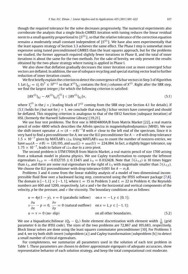
Fig. 3. Performance of different solution strategies for Problems 3(a) and 3(b): preconditionedmatrix–vector product counts of

the inner iteration against the outer iteration.

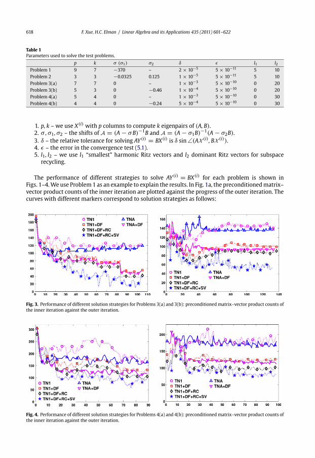
Fig. 4. Performance of different solution strategies for Problems 4(a) and 4(b): preconditionedmatrix–vector product counts of

the inner iteration against the outer iteration.


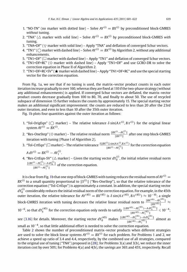
1. “NO-TN” (no marker with dotted line) – Solve AY (i) = BX(i) by preconditioned block-GMRES

without tuning.

2. “TNA” (� marker with solid line) – Solve AY (i) = BX(i) by preconditioned block-GMRES with

tuning.

3. “TNA+DF” (� marker with solid line) – Apply “TNA” and deflation of converged Schur vectors.

4. “TN1” (©markerwith dashed line) – Solve AY (i) = BX(i) by Algorithm 2, without any additional

enhancements.

5. “TN1+DF” (� marker with dashed line) – Apply “TN1” and deflation of converged Schur vectors.

6. “TN1+DF+RC” (♦ marker with dashed line) – Apply “TN1+DF” and use GCRO-DR to solve the

correction equation in Phase II of Algorithm 2.

7. “TN1+DF+RC+SV” (�markerwishdashed line) –Apply “TN1+DF+RC” anduse the special starting

vector for the correction equation.

From Fig. 1a, we see that if no tuning is used, the matrix–vector product counts in each outer

iteration increasegradually toover160,whereas theyarefixedat110 if the two-phase strategy (without

any additional enhancements) is applied. If converged Schur vectors are deflated, the matrix–vector

product counts decrease gradually from 100 to 80, 70, and finally to about 50. The use of recycled

subspace of dimension 15 further reduces the counts by approximately 15. The special starting vector

makes an additional significant improvement: the counts are reduced to less than 20 after the 23rd

outer iteration, and even to less than 10 after the 35th outer iteration.

Fig. 1b plots four quantities against the outer iteration as follows:

1. “Tol-OrigEqn” (© marker) – The relative tolerance δ sin(AX (i), BX (i)) for the original linear

system AY (i) = BX(i).

2. “Res-OneStep” (♦marker) – The relative residual norm‖BX(i)−AY

(i)1 ‖

‖BX(i)‖ after one step block-GMRES

iteration with tuning (Phase I of Algorithm 2).

3. “Tol-CrtEqn” (�marker) – The relative toleranceδ‖BX(i)‖ sin(AX (i) ,BX (i))

‖BX(i)−AY(i)1 ‖ for the correction equation

A dY (i) = BX(i) − AY(i)1 .

4. “Res-CrtEqn-SV” (� marker) – Given the starting vector dY(i)0 , the initial relative residual norm

‖(BX(i)−AY(i)1 )−A dY

(i)0 ‖

‖BX(i)−AY(i)1 ‖ of the correction equation.

It is clear fromFig. 1b thatone stepofblock-GMRESwith tuning reduces the residualnormofAY (i) =BX(i) to a small quantity proportional to ‖S(i)‖ (“Res-OneStep”), so that the relative tolerance of the

correction equation (“Tol-CrtEqn”) is approximately a constant. In addition, the special starting vector

dY(i)0 considerably reduces the initial residual normof the correction equation. For example, in the 45th

outer iteration, the relative tolerance for AY (45) = BX(45) is δ sin(AX (45), BX (45)) ≈ 10−10; a single

block-GMRES iteration with tuning decreases the relative linear residual norm to‖BX(45)−AY

(45)1 ‖

‖BX(45)‖ ≈10−6, so that dY

(45)k for the correction equation only needs to satisfy

‖(BX(45)−AY(45)1 )−A dY

(45)k ‖

‖BX(45)−AY(45)1 ‖ � 10−4;

see (3.16) for details. Moreover, the starting vector dY(45)0 makes

‖(BX(45)−AY(45)1 )−A dY

(45)0 ‖

‖BX(45)−AY(45)1 ‖ almost as

small as 10−4, so that little additional effort is needed to solve the correction equation.

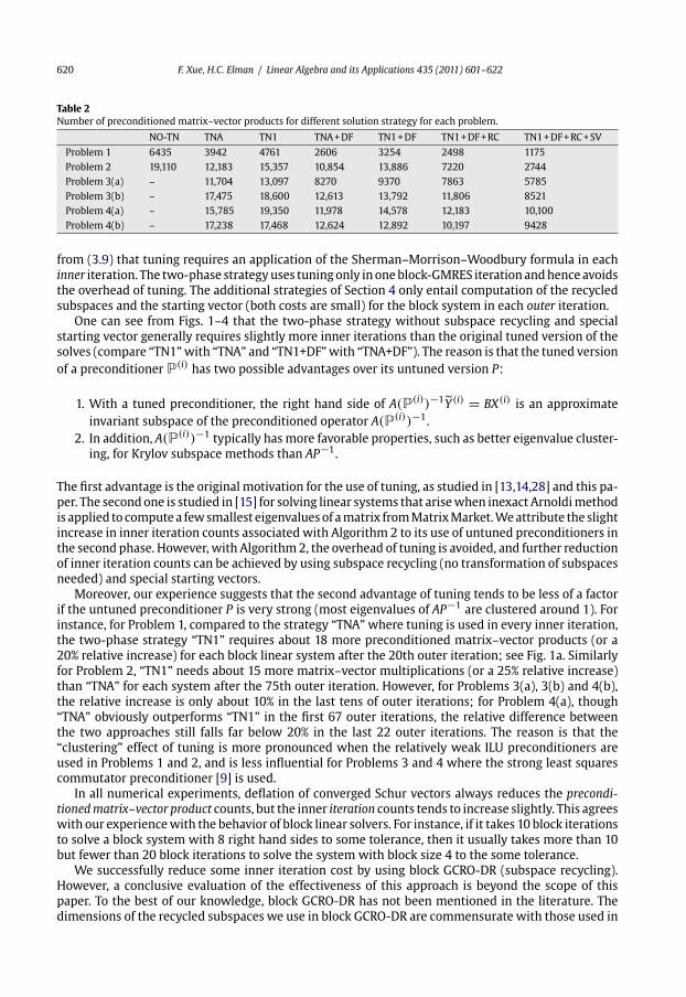
Table 2 shows the number of preconditioned matrix–vector products when different strategies

are used to solve the block linear systems AY (i) = BX(i) for each problem. For Problems 1 and 2, we

achieve a speed up ratio of 3.4 and 4.4, respectively, by the combined use of all strategies, compared

to the original use of tuning (“TNA”) proposed in [28]; for Problems 3(a) and 3(b), we reduce the inner

iteration cost by over 50%; for Problems 4(a) and 4(b), the savings are 36% and 45%, respectively. Recall


Table 2

Number of preconditioned matrix–vector products for different solution strategy for each problem.

NO-TN TNA TN1 TNA+DF TN1+DF TN1+DF+RC TN1+DF+RC+SV

Problem 1 6435 3942 4761 2606 3254 2498 1175

Problem 2 19,110 12,183 15,357 10,854 13,886 7220 2744

Problem 3(a) – 11,704 13,097 8270 9370 7863 5785

Problem 3(b) – 17,475 18,600 12,613 13,792 11,806 8521

Problem 4(a) – 15,785 19,350 11,978 14,578 12,183 10,100

Problem 4(b) – 17,238 17,468 12,624 12,892 10,197 9428

from (3.9) that tuning requires an application of the Sherman–Morrison–Woodbury formula in each

inner iteration. The two-phase strategyuses tuningonly inoneblock-GMRES iterationandhence avoids

the overhead of tuning. The additional strategies of Section 4 only entail computation of the recycled

subspaces and the starting vector (both costs are small) for the block system in each outer iteration.

One can see from Figs. 1–4 that the two-phase strategy without subspace recycling and special

starting vector generally requires slightly more inner iterations than the original tuned version of the

solves (compare “TN1”with “TNA” and “TN1+DF”with “TNA+DF”). The reason is that the tuned version

of a preconditioner P(i) has two possible advantages over its untuned version P:

1. With a tuned preconditioner, the right hand side of A(P(i))−1Y (i) = BX(i) is an approximate

invariant subspace of the preconditioned operator A(P(i))−1.

2. In addition, A(P(i))−1 typically has more favorable properties, such as better eigenvalue cluster-

ing, for Krylov subspace methods than AP−1.

The first advantage is the original motivation for the use of tuning, as studied in [13,14,28] and this pa-

per. The second one is studied in [15] for solving linear systems that arisewhen inexact Arnoldimethod

is applied to computea fewsmallest eigenvaluesof amatrix fromMatrixMarket.Weattribute the slight

increase in inner iteration counts associated with Algorithm 2 to its use of untuned preconditioners in

the second phase. However, with Algorithm2, the overhead of tuning is avoided, and further reduction

of inner iteration counts can be achieved by using subspace recycling (no transformation of subspaces

needed) and special starting vectors.

Moreover, our experience suggests that the second advantage of tuning tends to be less of a factor

if the untuned preconditioner P is very strong (most eigenvalues of AP−1 are clustered around 1). For

instance, for Problem 1, compared to the strategy “TNA” where tuning is used in every inner iteration,

the two-phase strategy “TN1” requires about 18 more preconditioned matrix–vector products (or a

20% relative increase) for each block linear system after the 20th outer iteration; see Fig. 1a. Similarly

for Problem 2, “TN1” needs about 15 more matrix–vector multiplications (or a 25% relative increase)

than “TNA” for each system after the 75th outer iteration. However, for Problems 3(a), 3(b) and 4(b),

the relative increase is only about 10% in the last tens of outer iterations; for Problem 4(a), though

“TNA” obviously outperforms “TN1” in the first 67 outer iterations, the relative difference between

the two approaches still falls far below 20% in the last 22 outer iterations. The reason is that the

“clustering” effect of tuning is more pronounced when the relatively weak ILU preconditioners are

used in Problems 1 and 2, and is less influential for Problems 3 and 4 where the strong least squares

commutator preconditioner [9] is used.

In all numerical experiments, deflation of converged Schur vectors always reduces the precondi-

tionedmatrix–vector product counts, but the inner iteration counts tends to increase slightly. This agrees

with our experiencewith the behavior of block linear solvers. For instance, if it takes 10 block iterations

to solve a block system with 8 right hand sides to some tolerance, then it usually takes more than 10

but fewer than 20 block iterations to solve the system with block size 4 to the some tolerance.

We successfully reduce some inner iteration cost by using block GCRO-DR (subspace recycling).

However, a conclusive evaluation of the effectiveness of this approach is beyond the scope of this

paper. To the best of our knowledge, block GCRO-DR has not been mentioned in the literature. The

dimensions of the recycled subspaces we use in block GCRO-DR are commensurate with those used in


single-vector GCRO-DR [27]. Since block GCRO-DR generally needs much bigger subspaces to extract

candidate solutions than its single-vector counterpart, it might be beneficial to use recycled subspaces

of bigger dimensions. In addition, the harmonic Ritz vectors corresponding to smallest harmonic Ritz

values are not necessarily a good choice for recycling if, for example, the smallest eigenvalues of the

preconditioned system matrix are not well-separated from other eigenvalues [5]. We speculate this

is the case in Problems 3 and 4, where there are several very small eigenvalues and some small ones

when the least squares commutator preconditioner is used (see [9]). In this case, it is the dominant

Ritz vectors that are useful.

6. Conclusion

Wehave studied inexact subspace iteration for solving generalizednon-Hermitian eigenvalueprob-

lemswith shift-invert and Cayley transformations.Weprovide newperspectives on tuning and discuss

the connection of the two-phase strategy to the inverse correctionmethod, the residual inverse power

method and the Jacobi–Davidson method. The two-phase strategy applies tuning only in the first

block-GMRES iteration and solves the correction equation with a fixed relative tolerance. It prevents

the inner iteration counts from increasing as the outer iteration proceeds, as the original approach in

[28] does. Three additional strategies are studied to further reduce the inner iteration cost, including

deflation, subspace recycling and special initial guess. Numerical experiments show clearly that the

combined use of all these techniques leads to significant reduction of inner iteration counts.

Acknowledgement

We thank the reviewers for a very careful reading of the manuscript.

References

[1] J. Berns-Müller, A. Spence, Inexact Inverse Iteration andGMRES, Tech Reportmaths0507, University of Bath, Bath, UK, 2005.[2] J. Berns-Müller, A. Spence, Inexact inverse iterationwith variable shift for nonsymmetric generalized eigenvalue problems,

SIAM J. Matrix Anal. Appl. 28 (4) (2006) 1069–1082.[3] J. Berns-Müller, I.G. Graham, A. Spence, Inexact inverse iteration for symmetric matrices, Linear Algebra Appl. 416 (2–3)

(2006) 389–413.[4] K.A. Cliffe, T.J. Garratt, A. Spence, Eigenvalues of block matrices arising from problems in fluid mechanics, SIAM J. Matrix

Anal. 15 (4) (1994) 1310–1318.[5] E. de Sturler, Private communication, October 2008.[6] E. de Sturler, Truncation strategies for optimal Krylov subspace methods, SIAM J. Numer. Anal. 36 (3) (1999) 864–889.[7] H.C. Elman, A.R. Ramage, D.J. Silvester, A.J. Wathen, Incompressible Flow Iterative Solution Software Package. Available

from: <http://www.cs.umd.edu/elman/ifiss.html>.[8] H.C. Elman,A.R. Ramage,D.J. Silvester, IFISS: aMatlab toolbox formodelling incompressibleflow,ACMTrans.Math. Software

33 (2) (2007) 18, Article 14.[9] H.C. Elman,D.J. Silvester,A.J.Wathen,Performanceandanalysisof saddlepointpreconditioners for thediscrete steady-state

Navier–Stokes equations, Numer. Math. 90 (4) (2002) 665–688.[10] H.C. Elman, D.J. Silvester, A.J. Wathen, Finite Elements and Fast Iterative Solvers, Oxford University Press, New York, 2005.[11] O.G. Ernst, Residual-minimizing Krylov subspacemethods for stabilized discretizations of convection–diffusion equations,

SIAM J. Matrix Anal. Appl. 21 (4) (2000) 1079–1101.[12] M. Freitag, A. Spence, A tuned preconditioner for inexact inverse iteration applied to Hermitian eigenvalue problems, IMA

J. Numer. Anal. 28 (3) (2007) 522–551.[13] M. Freitag, A. Spence, Convergence rates for inexact inverse iteration with application to preconditioned iterative solves,

BIT Numer. Math. 47 (1) (2007) 27–44.[14] M. Freitag, A. Spence, Rayleigh quotient iteration and simplified Jacobi–Davidson method with preconditioned iterative

solves, Linear Algebra Appl. 428 (8–9) (2008) 2049–2060.[15] M. Freitag, A. Spence, Shift-invert Arnoldi’s method with preconditioned iterative solves, SIAM J. Matrix Anal. Appl. 31 (3)

(2009) 942–969.[16] G.H. Golub, C.F. van Loan, Matrix Computations, third ed., The Johns Hopskins University Press, Baltimore, 1996.[17] G. Golub, Q. Ye, Inexact inverse iteration for generalized eigenvalue problems, BIT Numer. Math. 40 (4) (2000) 671–684.[18] M. Hochbruck, C. Lubich, On Krylov subspace approximations to the matrix exponential operator, SIAM J. Numer. Anal. 34

(5) (1997) 1911–1925.[19] HSL. Available from: <http://www.cse.scitech.ac.uk/nag/hsl/>.[20] Y. Lai, K. Lin, W. Lin, An inexact inverse iteration for large sparse eigenvalue problems, Numer. Linear Algebra Appl. 4 (5)

(1997) 425–437.[21] R.B. Lehoucq, J.A. Scott, An Evaluation of Subspace Iteration Software for Sparse Nonsymmetric Eigenvalue Problems,

RAL-TR-96-022, Rutherford Appleton Lab., 1996.

http://www.cs.umd.edu/elman/ifiss.html

http://www.cse.scitech.ac.uk/nag/hsl/


[22] Matrix Market. Available from: <http://math.nist.gov/MatrixMarket/>.[23] K. Meerbergen, A. Spence, D. Roose, Shift-invert and Cayley transforms for detection of rightmost eigenvalues of

nonsymmetric matrices, BIT Numer. Math. 34 (3) (1994) 409–423.[24] R.B. Morgan, GMRES with deflated restarting, SIAM J. Sci. Comput. 24 (1) (2002) 20–37.[25] R.B. Morgan, Restarted block-GMRES with deflation of eigenvalues, Appl. Numer. Math. 54 (2) (2005) 222–236.[26] Y. Notay, Convergence analysis of inexact Rayleigh quotient iteration, SIAM J. Matrix Anal. Appl. 24 (3) (2003) 627–644.[27] M.L. Parks, E. De Sturler, G. Mackey, D.D. Johnson, S. Maiti, Recycling Krylov subspaces for sequences of linear systems,

SIAM J. Sci. Comput. 28 (5) (2006) 1651–1674.[28] M. Robbé, M. Sadkane, A. Spence, Inexact inverse subspace iteration with preconditioning applied to non-Hermitian

eigenvalue problems, SIAM J. Matrix Anal. Appl. 31 (1) (2009) 92–113.[29] U. Rüde, W. Schmid, Inverse Multigrid Correction for Generalized Eigenvalue Computations, Technical Report 338,

Universität Augsburg, 1995.[30] Y. Saad, Iterative Methods for Sparse Linear Systems, second ed., SIAM, Philadelphia, 2003.[31] V. Simoncini, L. Eldén, Inexact Rayleigh quotient-type methods for eigenvalue computations, BIT Numer. Math. 42 (1)

(2002) 159–182.[32] P. Smit,M.H.C. Paardekooper, The effects of inexact solvers in algorithms for symmetric eigenvalueproblems,LinearAlgebra

Appl. 287 (1999) 337–357.[33] G.W. Stewart, Matrix Algorithms Volumn II: Eigensystems, SIAM, Philadelphia, 2001.[34] G.W. Stewart, A Residual Inverse Power Method, UMIACS TR-2007-09, CMSC TR-4890, University of Maryland, 2007.

http://math.nist.gov/MatrixMarket/

Documents

Linear Algebra and its Applications - UMD Department of ...elman/papers/subsp_iter.pdf · Linear Algebra and its Applications 435 (2011) 601–622 Contents lists available at ScienceDirect