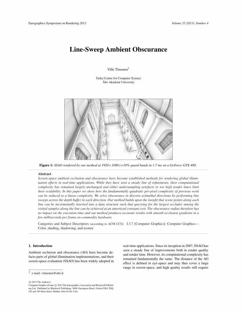
Eurographics Symposium on Rendering 2013 Volume 32 (2013), Number 4

Line-Sweep Ambient Obscurance

Ville Timonen†

Turku Centre for Computer ScienceÅbo Akademi University

Figure 1: SSAO rendered by our method at 1920×1080 (+10% guard band) in 1.7 ms on a GeForce GTX 480.

Abstract

Screen-space ambient occlusion and obscurance have become established methods for rendering global illumi-

nation effects in real-time applications. While they have seen a steady line of refinements, their computational

complexity has remained largely unchanged and either undersampling artefacts or too high render times limit

their scalability. In this paper we show how the fundamentally quadratic per-pixel complexity of previous work

can be reduced to a linear complexity. We solve obscurance in discrete azimuthal directions by performing line

sweeps across the depth buffer in each direction. Our method builds upon the insight that scene points along each

line can be incrementally inserted into a data structure such that querying for the largest occluder among the

visited samples along the line can be achieved at an amortized constant cost. The obscurance radius therefore has

no impact on the execution time and our method produces accurate results with smooth occlusion gradients in a

few milliseconds per frame on commodity hardware.

Categories and Subject Descriptors (according to ACM CCS): I.3.7 [Computer Graphics]: Computer Graphics—Color, shading, shadowing, and texture

1. Introduction

Ambient occlusion and obscurance (AO) have become de-facto parts of global illumination implementations, and theirscreen-space evaluation (SSAO) has been widely adopted in

† e-mail: vtimonen@abo.fi

real-time applications. Since its inception in 2007, SSAO hasseen a steady line of improvements both in render qualityand render time. However, its computational complexity hasremained fundamentally the same. The distance of the AOeffect is defined in eye-space and may thus cover a largerange in screen-space, and high quality results still require

c© 2013 The Author(s)Computer Graphics Forum c© 2013 The Eurographics Association and Blackwell Publish-ing Ltd. Published by Blackwell Publishing, 9600 Garsington Road, Oxford OX4 2DQ,UK and 350 Main Street, Malden, MA 02148, USA.

V. Timonen / LSAO

more samples per pixel than is practically affordable in real-time applications.

One established SSAO method is Horizon-Based Ambi-ent Occlusion (HBAO) [BSD08] [Bav11] which accumu-lates obscurance from a set of azimuthal directions, findingthe largest occluder in each direction by ray marching. WhileHBAO’s physically based treatment of geometry scales wellquality-wise, the number of samples that is necessary in eachazimuthal direction for high quality results is prohibitiveperformance-wise. Given K azimuthal directions and N stepsalong each direction, HBAO’s time complexity per pixel isO(KN).

We propose a method to calculate the same results inO(K) time with unlimited range. Instead of calculating theobscurance independently for each receiver pixel, we per-form line sweeps over the screen. Each line is traversed in-crementally, and the visited geometry along the line is storedin an internal data structure which can be queried in amor-tized constant time for the largest falloff attenuated occluderat the new pixel. This significant reduction in the time com-plexity of SSAO allows the fast production of high qualityrenderings which is not impacted by the range of the effect.Since we are not allowed to choose the azimuthal directionsfor each pixel freely, but rather use a set of directions sharedby multiple screen pixels, our main visual artefact is bandingwhich can be alleviated by increasing K.

2. Previous Work

Evaluating AO from the geometry in the depth buffer wasfirst proposed by [Mit07] and [SA07] who sample a vol-ume around the receiver pixel and determine the occlusionfrom the number of points that fall below the depth field. Asscene geometry not merely blocks incoming light but alsoreflects it, an empirically selected falloff function [ZIK98] isusually introduced that weighs the sampled scene points ac-cording to their distance from the receiver by putting moreweight to nearby occluders. Ambient occlusion extendedby a falloff function has been termed ambient obscurance.Since [Mit07] and [SA07], several works such as [BS09][LS10] [MOBH11] [MML12] have refined the quality andrendering speed of SSAO methods.

Evaluating each sampled scene point independently fromeach other ignores the fact that the evaluation of occludersin roughly the same azimuthal direction is not separable: Atall nearby occluder might make occluders behind it invisiblesuch that these do not contribute to occlusion regardless oftheir elevation. To address this issue [BSD08] takes a morephysically based approach along the lines of Horizon Map-ping [Max88], whereby the highest horizon within a certainrange is searched for a set of azimuthal directions. Whilethis approach scales well with respect to image quality andobscurance radius, it is expensive because many height fieldsamples have to be taken in each azimuthal direction. Our

method produces results essentially identical to [BSD08] butwe find the largest occluder in O(1) time for one azimuthaldirection within an unbounded radius.

We build upon the observation by [TW10] that sweepingthrough a height field in lines and incrementally buildingthe convex hull of the visited geometry allows the extrac-tion of global horizons in constant time for the purpose ofhorizon mapping. In ambient obscurance, where the fallofffunction attenuates occlusion with distance, the global hori-zon is often very far away and contributes little to occlu-sion, making the convex hull of little use in determining AO.Also, [TW10] scans the height field densely and accumu-lates rotated versions of the sweeps. This results in bandingunless many azimuthal directions are scanned, which in turnbecomes computationally expensive.

Our contribution over [TW10] is three-fold:

• Instead of using a geometrical convex hull, we form a hullbased on the falloff weighted obscurance.

• We generalize the scans to arbitrary sampling densi-ties and propose a way to gather results sparsely per-pixel, which allows trading high render times for edge-respecting blur when the number of azimuthal scanningdirections is increased.

• We also suggest special line sampling patterns for caseswhere depth buffer values cannot be interpolated (oftenthe case in SSAO).

3. Overview

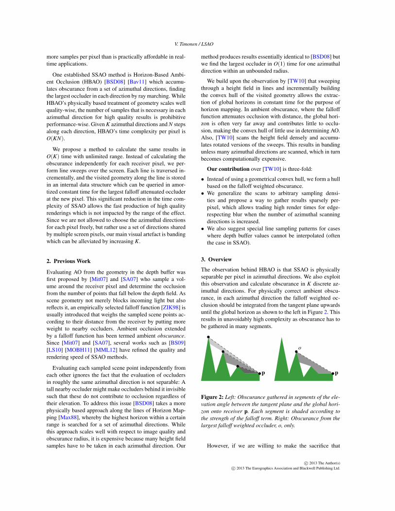
The observation behind HBAO is that SSAO is physicallyseparable per pixel in azimuthal directions. We also exploitthis observation and calculate obscurance in K discrete az-imuthal directions. For physically correct ambient obscu-rance, in each azimuthal direction the falloff weighted oc-clusion should be integrated from the tangent plane upwardsuntil the global horizon as shown to the left in Figure 2. Thisresults in unavoidably high complexity as obscurance has tobe gathered in many segments.

p p

o

Figure 2: Left: Obscurance gathered in segments of the ele-

vation angle between the tangent plane and the global hori-

zon onto receiver p. Each segment is shaded according to

the strength of the falloff term. Right: Obscurance from the

largest falloff weighted occluder, o, only.

However, if we are willing to make the sacrifice that

c© 2013 The Author(s)c© 2013 The Eurographics Association and Blackwell Publishing Ltd.

V. Timonen / LSAO

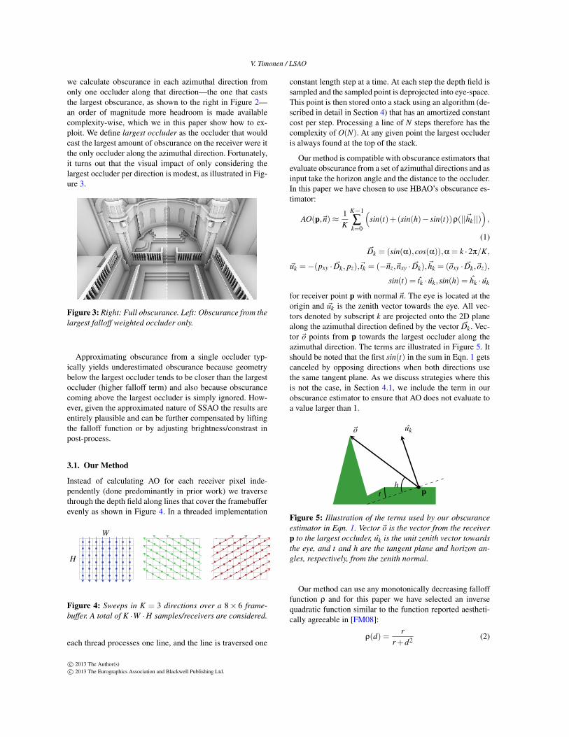
we calculate obscurance in each azimuthal direction fromonly one occluder along that direction—the one that caststhe largest obscurance, as shown to the right in Figure 2—an order of magnitude more headroom is made availablecomplexity-wise, which we in this paper show how to ex-ploit. We define largest occluder as the occluder that wouldcast the largest amount of obscurance on the receiver were itthe only occluder along the azimuthal direction. Fortunately,it turns out that the visual impact of only considering thelargest occluder per direction is modest, as illustrated in Fig-ure 3.

Figure 3: Right: Full obscurance. Left: Obscurance from the

largest falloff weighted occluder only.

Approximating obscurance from a single occluder typ-ically yields underestimated obscurance because geometrybelow the largest occluder tends to be closer than the largestoccluder (higher falloff term) and also because obscurancecoming above the largest occluder is simply ignored. How-ever, given the approximated nature of SSAO the results areentirely plausible and can be further compensated by liftingthe falloff function or by adjusting brightness/constrast inpost-process.

3.1. Our Method

Instead of calculating AO for each receiver pixel inde-pendently (done predominantly in prior work) we traversethrough the depth field along lines that cover the framebufferevenly as shown in Figure 4. In a threaded implementation

W

H

Figure 4: Sweeps in K = 3 directions over a 8× 6 frame-

buffer. A total of K ·W ·H samples/receivers are considered.

each thread processes one line, and the line is traversed one

constant length step at a time. At each step the depth field issampled and the sampled point is deprojected into eye-space.This point is then stored onto a stack using an algorithm (de-scribed in detail in Section 4) that has an amortized constantcost per step. Processing a line of N steps therefore has thecomplexity of O(N). At any given point the largest occluderis always found at the top of the stack.

Our method is compatible with obscurance estimators thatevaluate obscurance from a set of azimuthal directions and asinput take the horizon angle and the distance to the occluder.In this paper we have chosen to use HBAO’s obscurance es-timator:

AO(p,~n)≈1K

K−1

∑k=0

(

sin(t)+(sin(h)− sin(t))ρ(||~hk||))

,

(1)

~Dk = (sin(α),cos(α)),α = k ·2π/K,

~uk =−(pxy · ~Dk, pz),~tk = (−~nz,~nxy · ~Dk), ~hk = (~oxy · ~Dk,~oz),

sin(t) = tk · uk,sin(h) = hk · uk

for receiver point p with normal~n. The eye is located at theorigin and ~uk is the zenith vector towards the eye. All vec-tors denoted by subscript k are projected onto the 2D planealong the azimuthal direction defined by the vector ~Dk. Vec-tor ~o points from p towards the largest occluder along theazimuthal direction. The terms are illustrated in Figure 5. Itshould be noted that the first sin(t) in the sum in Eqn. 1 getscanceled by opposing directions when both directions usethe same tangent plane. As we discuss strategies where thisis not the case, in Section 4.1, we include the term in ourobscurance estimator to ensure that AO does not evaluate toa value larger than 1.

~o

p

uk

ht

Figure 5: Illustration of the terms used by our obscurance

estimator in Eqn. 1. Vector ~o is the vector from the receiver

p to the largest occluder, uk is the unit zenith vector towards

the eye, and t and h are the tangent plane and horizon an-

gles, respectively, from the zenith normal.

Our method can use any monotonically decreasing fallofffunction ρ and for this paper we have selected an inversequadratic function similar to the function reported aestheti-cally agreeable in [FM08]:

ρ(d) =r

r+d2 (2)

c© 2013 The Author(s)c© 2013 The Eurographics Association and Blackwell Publishing Ltd.

V. Timonen / LSAO

where r is used to control the decay rate.

The obscurance results written along the processed linesare gathered per pixel in a separate phase, described in Sec-tion 5. In Section 5 we also cover how lines are positionedin the framebuffer and how sampling coordinates should bechosen. Rendered images and execution times are then pre-sented in Section 6 and compared against the most relevantprevious work.

4. Line Sweeping

In this section we describe the process of sweeping throughone line in the framebuffer. The output of this process areobscurance values for the points along the line written to anintermediate buffer.

4.1. Obscurance Hull

We first recapitulate the main idea behind incremental con-

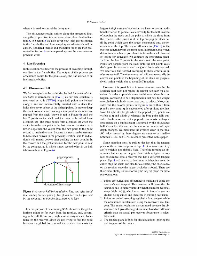
vex hulls as introduced in [TW10] as our data structure ismotivated by it. In [TW10] height field points are iteratedalong a line and incrementally inserted onto a stack thatholds the convex subset of the visited points. In order to keepthe stack convex before pushing a new point in, elements arepopped from the stack (shown in red in Figure 6) until thelast 2 points on the stack and the point to be added forma convex set. The three points form a convex set when thevector from the new point to the last point on the stack has alower slope than the vector from the new point to the pointsecond to last in the stack. Because the stack can be assumedto have been convex in the previous iteration, due to induc-tion it will remain convex after pushing the new point in. Inthe convex hull the global horizon for the new point is castby the point next to it, which is now second to last in the hull(shown in blue in Figure 6).

ppopped points

direction of line sweep

Figure 6: A convex hull before (dashed line) and after (solid

line) adding the new point p. The global horizon for p is cast

by the point next to it in the hull, marked in blue.

For the purpose of determining SSAO however, the globalhorizon might be far away from the receiver, and, accord-ing to the falloff function, might cast an insignificant obscu-rance on the receiver. Since we are trying to find the pointbetween the global horizon and the receiver that casts the

largest falloff weighted occlusion we have to use an addi-tional criterion to geometrical convexity for the hull. Insteadof popping the stack until the point to which the slope fromthe receiver is the lowest is at the top, we pop the stack un-til the point which casts the largest obscurance onto the re-ceiver is at the top. The main difference to [TW10] is theboolean function (with the three points as parameters) whichdetermines whether to pop elements from the stack: Insteadof testing for convexity, we compare the obscurance (Eqn.1) from the last 2 points in the stack onto the new point.Points are popped from the stack until the last points caststhe largest obscurance, or until the global horizon is reached.We refer to a hull formed according to these criteria as anobscurance hull. The obscurance hull will not necessarily beconvex and points in the beginning of the stack are progres-sively losing weight due to the falloff function.

However, it is possible that in some extreme cases the ob-scurance hull does not return the largest occluder for a re-ceiver. In order to provide some intuition on when this canhappen, consider ρ to be a step function that puts full weightto occluders within distance r and zero to others. Next, con-sider that the colored points in Figure 6 are within r fromp and a new point, q, is encountered after p along the line.Now, let q be at a height where the popped (red) points arevisible to q and within r, whereas the blue point falls out-side r. In this case one of the popped points casts the largestobscurance on q but instead p is returned by the obscurancehull. Cases like this are rare but can occur in areas of rapiddepth changes. We measured the average error in the finalAO value caused by these degenerate cases to be small—between 0.02% and 0.3% in scenes presented in this paper.

Some attention must be paid to the fact that the tangentplane of the receiver appears in Eqn. 1. Obscurance is cut bysin(t) which is not globally fixed. Therefore forming an ob-scurance hull using one tangent plane might not give the cor-rect obscurance onto a receiver that has a different tangentplane. Eqn. 1 will be used to determine which points are to beculled atop the stack, and also for calculating the obscuranceon the receiver once the largest occluder is found. There arethree main strategies for choosing the tangent plane for thesetwo operations:

1. Points are culled and obscurance is calculated using thereceiver’s real tangent. This however will cause the ob-scurance hull to rapidly unfold when the tangent becomessteep (high sin(t)), which may result in future largest oc-cluders being culled and therefore in missing occlusion.

2. Points are culled assuming a globally fixed tangent whilethe obscurance is calculated using the receiver’s real tan-gent. This makes occlusion discontinued because the ob-scurance hull gives the largest occluder based on differentcriteria than the actual per-receiver obscurance is calcu-lated with.

3. The tangent plane is fixed for all calculations ignoring thereal tangents of the points.

c© 2013 The Author(s)c© 2013 The Eurographics Association and Blackwell Publishing Ltd.

V. Timonen / LSAO

reference

error ×2

Hull: real tangent,

Occ: real tangent:1.

error ×2

Hull: sin(t) = 0.0,

Occ: real tangent:2.

error ×2

Hull: sin(t) =−0.5,

Occ: real tangent:

error ×2

Hull: sin(t) =−0.5,

Occ: sin(t) =−0.5:3.

error ×2

Hull: sin(t) =−1.0,

Occ: sin(t) =−1.0:

a b c

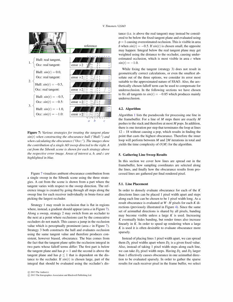
Figure 7: Various strategies for treating the tangent plane

sin(t) when constructing the obscurance hull ("Hull:") and

when calculating the obscurance ("Occ:"). The images show

the contribution of a single AO sweep directed to the right. A

cut from the Sibenik scene is shown for each strategy above

the respective error image. Areas of interest a, b, and c are

highlighted in blue.

Figure 7 visualizes ambient obscurance contribution froma single sweep in the Sibenik scene using the three strate-gies. A cut from the scene is shown from a part where thetangent varies with respect to the sweep direction. The ref-erence image is created by going through all steps along thesweep line for each receiver individually in brute-force andpicking the largest occluder.

Strategy 1 may result in occlusion that is flat in regionswhere, instead, a gradient should appear (area a in Figure 7).Along a sweep, strategy 2 may switch from an occluder tothe next at a point where occlusions cast by the consecutiveoccluders do not match. This causes a jump in the occlusionvalue which is perceptually prominent (area c in Figure 7).Strategy 3 both constructs the hull and evaluates occlusionusing the same tangent value and therefore produces con-sistent, however biased, obscurance. The bias comes fromthe fact that the tangent plane splits the occlusion integral intwo parts whose falloff terms differ: The first part is belowthe tangent plane and has ρ = 1 and the second is above thetangent plane and has ρ ≤ 1 that is dependent on the dis-tance to the occluder. If sin(t) is chosen large, part of theintegral that should be evaluated using the occluder’s dis-

tance (i.e. is above the real tangent) may instead be consid-ered to be below the fixed tangent plane and evaluated usingρ= 1 causing overestimated occlusion. This is visible in areab when sin(t) =−0.5. If sin(t) is chosen small, the oppositemay happen: Integral below the real tangent plane may getweighted using the distance to the occluder, causing under-estimated occlusion, which is most visible in area c whensin(t) =−1.0.

While fixing the tangent (strategy 3) does not result ingeometrically correct calculations, or even the smallest ab-solute out of the three options, we consider its error mostsuitable to the approximated nature of SSAO. Also, the aes-thetically chosen falloff term can be used to compensate forunderocclusion. In the following sections we have chosento fix all tangents to sin(t) =−0.85 which produces mainlyunderocclusion.

4.2. Algorithm

Algorithm 1 lists the pseudocode for processing one line inthe framebuffer. For a line of M steps there are exactly M

pushes to the stack and therefore at most M pops. In addition,there is one iteration per step that terminates the loop at lines12 – 18 without causing a pop, which results in finding thepoint that casts the highest obscurance. Therefore the innerloop will perform between M and 2M iterations in total andyields the time complexity of O(M) for the algorithm.

5. Gathering Line Sweep Results

In this section we cover how lines are spread out in theframebuffer, how sampling coordinates are selected alongthe lines, and finally how the obscurance results from pro-cessed lines are gathered per final rendered pixel.

5.1. Line Placement

In order to densely evaluate obscurance for each of the K

directions lines can be placed 1 pixel width apart and stepsalong each line can be chosen to be 1 pixel width long. As aresult obscurance is evaluated at W ·H pixels for each K di-rections (previously illustrated in Figure 4). Since the sameset of azimuthal directions is shared by all pixels, bandingmay become visible unless a large K is used. IncreasingK eventually hides banding, but render times also increaselinearly in K. In order to speed up rendering when a largeK is used it is often desirable to evaluate obscurance moresparsely.

Instead of placing lines 1 pixel width apart, we can spreadthem DL pixel widths apart where DL is a given fixed value.Also, instead of taking 1 pixel width steps along each line,we can take DS pixel width steps. Having DL and DS largerthan 1 effectively causes obscurance in one azimuthal direc-tion to be evaluated sparsely. In order to gather the sparseresults for each receiver pixel in the frame buffer, we select

c© 2013 The Author(s)c© 2013 The Eurographics Association and Blackwell Publishing Ltd.

V. Timonen / LSAO

Algorithm 1 SweepLine(float2 pos, float2 dir, int steps)Functions peek1() and peek2() return the last and the second

to last element of the stack, respectively.

1 while (steps−−)2 {3 float3 p = deProj(sampleDepth(pos))4 float2 pk = float2(p.xy · dir, p.z)56 // Unit vector towards the camera

7 float2 uk = −pk/||pk||89 float2 h1 = hull.peek1() − pk

10 float2 h2 = hull.peek2() − pk1112 while

(

occlusion(h1, uk) < occlusion(h2, uk) &&13 h1·uk/||h1|| < h2·uk/||h2||

)

14 {15 hull.pop()16 h1 = h217 h2 = hull.peek2() − pk18 }1920 writeResult(occlusion(h1, uk))21 hull.push(pk)22 pos += dir23 }2425 float occlusion(float2 h, float2 u)26 {27 // sin(t) = −0.85

28 return sin(t) + max(

0, h·u/||h||− sin(t))

·ρ(||h||)29 }

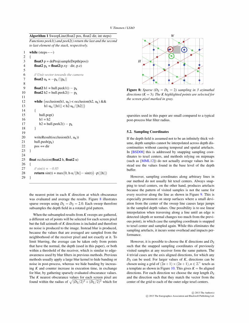
the nearest point in each K direction at which obscurancewas evaluated and average the results. Figure 8 illustratessparse sweeps using DL = DS = 2.0. Each sweep thereforesubsamples the depth field in a rotated grid pattern.

When the subsampled results from K sweeps are gathered,a different set of points will be selected for each screen pixelbut the full azimuth of K directions is included and thereforeno noise is produced to the image. Instead blur is produced,because the values that are averaged are sampled from theneighborhood of the receiver pixel and not exactly at it. Tolimit blurring, the average can be taken only from pointsthat have the normal, the depth (used in this paper), or bothwithin a threshold of the receiver, which is similar to edge-awareness used by blur filters in previous methods. Previousmethods usually apply a large blur kernel to hide banding ornoise in post-process, whereas we hide banding by increas-ing K and counter increase in execution time, in exchangefor blur, by gathering sparsely evaluated obscurance values.The K nearest obscurance values for each screen pixel arefound within the radius of

√

(DS/2)2 +(DL/2)2 which for

W

H

Figure 8: Sparse (DS = DL = 2) sampling in 3 azimuthal

directions (K = 3). The K highlighted points are selected for

the screen pixel marked in gray.

sparsities used in this paper are small compared to a typicalpost-process blur filter radius.

5.2. Sampling Coordinates

If the depth field is assumed not to be an infinitely thick vol-ume, depth samples cannot be interpolated across depth dis-continuities without causing temporal and spatial artefacts.In [BSD08] this is addressed by snapping sampling coor-dinates to texel centers, and methods relying on mipmaps(such as [MML12]) do not actually average values but in-stead use the values found in the base level of the depthbuffer.

However, sampling coordinates along arbitrary lines inour method do not usually hit texel centers. Always snap-ping to texel centers, on the other hand, produces artefactsbecause the pattern of visited samples is not the same forevery receiver along the line as shown in Figure 9. This isespecially prominent on steep surfaces where a small devi-ation from the center of the sweep line causes large jumpsin the sampled depth values. One possibility is to use linearinterpolation when traversing along a line until an edge isdetected (depth or normal changes too much from the previ-ous point), in which case the sampling coordinate is snappedto texel center and sampled again. While this eliminates thesampling artefacts, it incurs some overhead and impacts per-formance.

However, it is possible to choose the K directions and DS

such that the snapped sampling coordinates of previouslyvisited samples at any receiver form the same pattern. The4 trivial cases are the axis aligned directions, for which anyDS can be used. For larger values of K, directions can bechosen using a grid of (2n+1)× (2n+1),n ∈ Z

+ texels asa template as shown in Figure 10. This gives K = 8n aligneddirections. For each direction we choose the step length DS

and the direction such that they match the vector from thecenter of the grid to each of the outer edge texel centers.

c© 2013 The Author(s)c© 2013 The Eurographics Association and Blackwell Publishing Ltd.

V. Timonen / LSAO

W

H

Figure 9: The colored texels will be sampled when sampling

coordinates are snapped to texel centers. For two different

receivers along the line (in blue), the sampling patterns (in

red and green) relative to the receiver differ (1 left/0 down

and 2 left/1 down vs. 1 left/1 down and 2 left/1 down) and

show up as noise in the obscurance on slanted surfaces.

K = 8,DS = 1.41 K = 16,DS = 2.43

Figure 10: Aligned sampling patterns and their average step

length DS. The axis aligned directions use DS that is the av-

erage of the rest of the directions.

While this allows safe snapping of sampling coordinatesto texel centers, the average DS increases along with K. For-tunately this is not a problem, since increasing K is often off-set by making the sampling sparser (larger DS and DL) suchthat banding is traded for blur without increasing the exe-cution time. The average number of calculated obscurancevalues per pixel is K/(DS ·DL).

Choosing sampling directions according to the box pat-tern causes directions near the diagonals to be sampled moredensely. In order to avoid bias resulting from this, contri-bution along directions should be weighted according tothe azimuthal coverage of each direction, such that smallerweights are given to the diagonal directions. This will resultin slightly higher resolution sampling near the diagonals in-stead of bias.

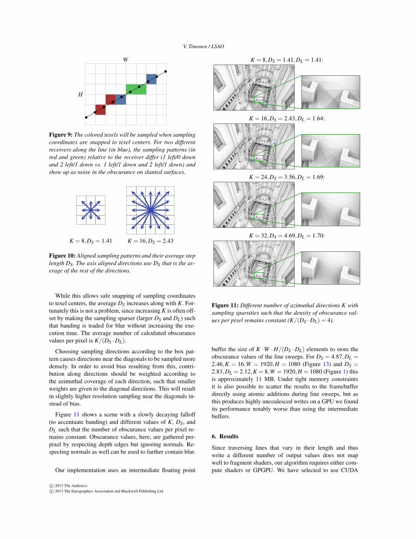
Figure 11 shows a scene with a slowly decaying falloff(to accentuate banding) and different values of K, DS, andDL such that the number of obscurance values per pixel re-mains constant. Obscurance values, here, are gathered per-pixel by respecting depth edges but ignoring normals. Re-specting normals as well can be used to further contain blur.

Our implementation uses an intermediate floating point

K = 8,DS = 1.41,DL = 1.41:

K = 16,DS = 2.43,DL = 1.64:

K = 24,DS = 3.56,DL = 1.69:

K = 32,DS = 4.69,DL = 1.70:

Figure 11: Different number of azimuthal directions K with

sampling sparsities such that the density of obscurance val-

ues per pixel remains constant (K/(DS ·DL) = 4).

buffer the size of K ·W ·H/(DS ·DL) elements to store theobscurance values of the line sweeps. For DS = 4.87,DL =2.46,K = 16,W = 1920,H = 1080 (Figure 13) and DS =2.83,DL = 2.12,K = 8,W = 1920,H = 1080 (Figure 1) thisis approximately 11 MB. Under tight memory constraintsit is also possible to scatter the results to the framebufferdirectly using atomic additions during line sweeps, but asthis produces highly uncoalesced writes on a GPU we foundits performance notably worse than using the intermediatebuffers.

6. Results

Since traversing lines that vary in their length and thuswrite a different number of output values does not mapwell to fragment shaders, our algorithm requires either com-pute shaders or GPGPU. We have selected to use CUDA

c© 2013 The Author(s)c© 2013 The Eurographics Association and Blackwell Publishing Ltd.

V. Timonen / LSAO

and made the sources available under the BSD license athttp://wili.cc/research/lsao/. The benchmarks areperformed on an NVidia GeForce GTX 480 GPU. TheHBAO method used as the reference is implemented as anOpenGL fragment shader. For quality and performance com-parison between HBAO and other recent SSAO methods, re-fer to [VPG13] and [McG10].

HBAO requires a falloff function that decays to 0, and wehave chosen the following falloff function for HBAO:

ρ0(d) = max

(

0,r (1+C)

r+d2 −C

)

(3)

This function has roughly the same shape as Eqn. 2 for smallC. Compared to Eqn. 2 it is sunken by C, clipped to 0, scaledto start from 1, and reaches zero at d =

√

r/C. In this sectionwe use C = 0.3.

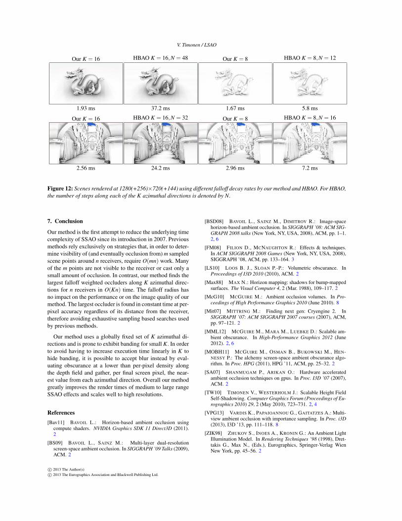
Figure 12 shows two scenes rendered at1280(+256)×720(+144) (20% guard band) using twodifferent rates of decay r for the falloff function. Ourmethod uses configurations for K = 8 and K = 16 shown inFigure 11, whereas the number of HBAO steps N have beenhand-picked for each scene and are scaled per-pixel to coverthe eye-space falloff radius. The execution time of HBAO isdifferent for the two falloff decay rates because a differentnumber of steps has to be taken to cover the bulk of thefalloff function with the same granularity. The executiontime of our method depends mainly on the variance in thenumber of iterations of the inner loop in Algorithm 1 withinwarps of threads, and does not vary significantly. In allscenes our method performs roughly 2K iterations per pixelon average (≈ K during line sweeps and K for gatheringthe results) whereas HBAO has to perform an order ofmagniture more, K ·N.

Table 1 shows scaling with respect to screen resolutionin the Sponza scene at K = 16 (bottom left in Figure 12).HBAO has to use larger N at higher resolutions to cover theeye-space falloff at the same screen-space accuracy, whereasour method has a constant per-pixel cost and scales linearlyin the resolution. The execution time of HBAO in fact in-

Table 1: Total render times of our method and HBAO at dif-

ferent resolutions using 20% guard band. The scene is shown

in Figure 12 to the bottom left.

Screen resolution Our method HBAO800×600 1.49 ms 10.5 ms1280×720 2.56 ms 24.2 ms1920×1080 5.24 ms 92.5 ms2560×1600 9.58 ms 249 ms

creases slightly faster than cubicly in the number of screenpixels because of increased texture cache misses, whereasthe slower than quadratic scaling in the execution time ofour method at lower screen resolutions is due to the small

number of threads (i.e. lines to sweep) which impacts hard-ware utilization. Our method takes very few texture samplesand is not much impacted by a texture cache miss penalty.

Our method consists of two stages: The line-sweep stageand the result gathering stage. Table 2 shows execution timebreakdown for these two stages when K is increased butK/(DS ·DL) is kept constant. Even though the amount of in-termediate sweep data stays the same, more data is read perpixel which shows up as a steady increase in the executiontime of the gather stage. Execution time of the line-sweepstage, on the other hand, decreases slightly because the workis split into a larger number of threads that run shorter, whichimproves hardware utilization.

Table 2: Render time breakdown per stage for our method

at 1280(+256)×720(+144) for cases shown in Figure 11.

Configuration Line-sweep GatherK = 8,DS = 1.41,DL = 1.41 1.91 ms 0.38 msK = 16,DS = 2.43,DL = 1.64 1.80 ms 0.59 msK = 24,DS = 3.56,DL = 1.69 1.67 ms 0.73 msK = 32,DS = 4.69,DL = 1.70 1.60 ms 0.90 ms

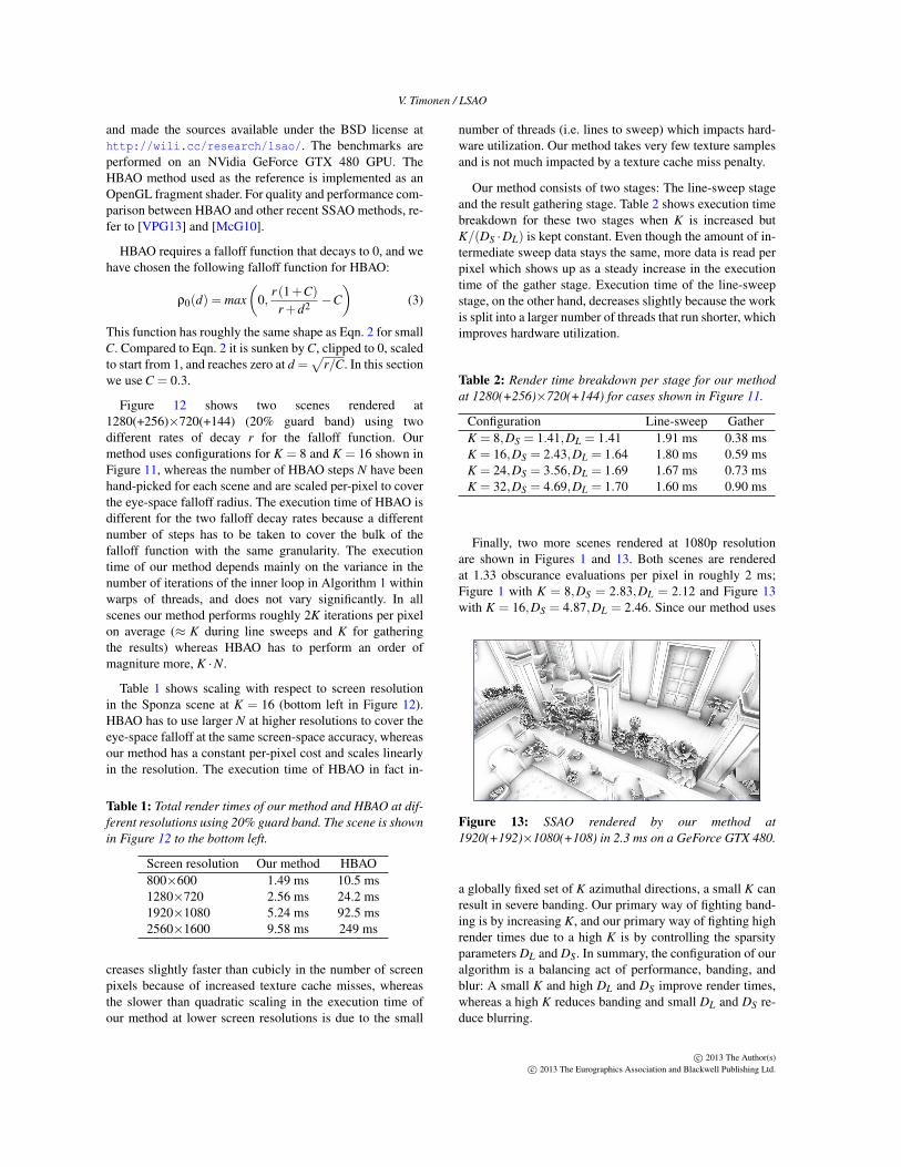
Finally, two more scenes rendered at 1080p resolutionare shown in Figures 1 and 13. Both scenes are renderedat 1.33 obscurance evaluations per pixel in roughly 2 ms;Figure 1 with K = 8,DS = 2.83,DL = 2.12 and Figure 13with K = 16,DS = 4.87,DL = 2.46. Since our method uses

Figure 13: SSAO rendered by our method at

1920(+192)×1080(+108) in 2.3 ms on a GeForce GTX 480.

a globally fixed set of K azimuthal directions, a small K canresult in severe banding. Our primary way of fighting band-ing is by increasing K, and our primary way of fighting highrender times due to a high K is by controlling the sparsityparameters DL and DS. In summary, the configuration of ouralgorithm is a balancing act of performance, banding, andblur: A small K and high DL and DS improve render times,whereas a high K reduces banding and small DL and DS re-duce blurring.

c© 2013 The Author(s)c© 2013 The Eurographics Association and Blackwell Publishing Ltd.

V. Timonen / LSAO

Our K = 16

2.56 ms

HBAO K = 16,N = 32

24.2 ms

Our K = 8

2.96 ms

HBAO K = 8,N = 16

7.2 ms

Our K = 16

1.93 ms

HBAO K = 16,N = 48

37.2 ms

Our K = 8

1.67 ms

HBAO K = 8,N = 12

5.8 ms

Figure 12: Scenes rendered at 1280(+256)×720(+144) using different falloff decay rates by our method and HBAO. For HBAO,

the number of steps along each of the K azimuthal directions is denoted by N.

7. Conclusion

Our method is the first attempt to reduce the underlying timecomplexity of SSAO since its introduction in 2007. Previousmethods rely exclusively on strategies that, in order to deter-mine visibility of (and eventually occlusion from) m sampledscene points around n receivers, require O(mn) work. Manyof the m points are not visible to the receiver or cast only asmall amount of occlusion. In contrast, our method finds thelargest falloff weighted occluders along K azimuthal direc-tions for n receivers in O(Kn) time. The falloff radius hasno impact on the performance or on the image quality of ourmethod. The largest occluder is found in constant time at per-pixel accuracy regardless of its distance from the receiver,therefore avoiding exhaustive sampling based searches usedby previous methods.

Our method uses a globally fixed set of K azimuthal di-rections and is prone to exhibit banding for small K. In orderto avoid having to increase execution time linearly in K tohide banding, it is possible to accept blur instead by eval-uating obscurance at a lower than per-pixel density alongthe depth field and gather, per final screen pixel, the near-est value from each azimuthal direction. Overall our methodgreatly improves the render times of medium to large rangeSSAO effects and scales well to high resolutions.

References

[Bav11] BAVOIL L.: Horizon-based ambient occlusion usingcompute shaders. NVIDIA Graphics SDK 11 Direct3D (2011).2

[BS09] BAVOIL L., SAINZ M.: Multi-layer dual-resolutionscreen-space ambient occlusion. In SIGGRAPH ’09 Talks (2009),ACM. 2

[BSD08] BAVOIL L., SAINZ M., DIMITROV R.: Image-spacehorizon-based ambient occlusion. In SIGGRAPH ’08: ACM SIG-

GRAPH 2008 talks (New York, NY, USA, 2008), ACM, pp. 1–1.2, 6

[FM08] FILION D., MCNAUGHTON R.: Effects & techniques.In ACM SIGGRAPH 2008 Games (New York, NY, USA, 2008),SIGGRAPH ’08, ACM, pp. 133–164. 3

[LS10] LOOS B. J., SLOAN P.-P.: Volumetric obscurance. InProceedings of I3D 2010 (2010), ACM. 2

[Max88] MAX N.: Horizon mapping: shadows for bump-mappedsurfaces. The Visual Computer 4, 2 (Mar. 1988), 109–117. 2

[McG10] MCGUIRE M.: Ambient occlusion volumes. In Pro-

ceedings of High Performance Graphics 2010 (June 2010). 8

[Mit07] MITTRING M.: Finding next gen: Cryengine 2. InSIGGRAPH ’07: ACM SIGGRAPH 2007 courses (2007), ACM,pp. 97–121. 2

[MML12] MCGUIRE M., MARA M., LUEBKE D.: Scalable am-bient obscurance. In High-Performance Graphics 2012 (June2012). 2, 6

[MOBH11] MCGUIRE M., OSMAN B., BUKOWSKI M., HEN-NESSY P.: The alchemy screen-space ambient obscurance algo-rithm. In Proc. HPG (2011), HPG ’11, ACM, pp. 25–32. 2

[SA07] SHANMUGAM P., ARIKAN O.: Hardware acceleratedambient occlusion techniques on gpus. In Proc. I3D ’07 (2007),ACM. 2

[TW10] TIMONEN V., WESTERHOLM J.: Scalable Height FieldSelf-Shadowing. Computer Graphics Forum (Proceedings of Eu-

rographics 2010) 29, 2 (May 2010), 723–731. 2, 4

[VPG13] VARDIS K., PAPAIOANNOU G., GAITATZES A.: Multi-view ambient occlusion with importance sampling. In Proc. i3D

(2013), I3D ’13, pp. 111–118. 8

[ZIK98] ZHUKOV S., INOES A., KRONIN G.: An Ambient LightIllumination Model. In Rendering Techniques ’98 (1998), Dret-takis G., Max N., (Eds.), Eurographics, Springer-Verlag WienNew York, pp. 45–56. 2

c© 2013 The Author(s)c© 2013 The Eurographics Association and Blackwell Publishing Ltd.