Line spread function - Argolight

1

Daybook Analysis – Version 1.8.0 – March 2021

Copyright 2021 by Argolight SA. All rights reserved. No part of this document may be used or reproduced in any form or stored in a database or retrieval system. Making copies of any part of this document for any purpose other than your own personal use is a violation of European copyright laws.

Line spread function

Table of contents

I. INTRODUCTION ................................................................................................................... 1

II. IMAGE ACQUISITION PROCEDURE ................................................................................... 2

1. ACQUISITION RECOMMENDATIONS ......................................................................................... 2

2. HOW TO IMAGE THE PATTERN? ............................................................................................... 3

III. IMAGE ANALYSIS PROCEDURE ......................................................................................... 5

1. HOW TO LAUNCH AN ANALYSIS? ............................................................................................. 5

2. ANALYSIS SETTINGS ................................................................................................................. 5

IV. RESULTS PAGE DESCRIPTION .......................................................................................... 9

1. INTERFACE ................................................................................................................................. 9

2. OPTIONS ..................................................................................................................................... 9

V. ANALYSIS ALGORITHM DESCRIPTION ........................................................................... 12

1. DIAGRAM ....................................................................................................................................12

2. DESCRIPTION ............................................................................................................................12

VI. OUTPUT METRIC DESCRIPTION ...................................................................................... 14

1. PRIMARY METRICS ...................................................................................................................14

2. SECONDARY METRICS .............................................................................................................14

3. ALGORITHM METADATA ...........................................................................................................15

4. IMAGE METADATA .....................................................................................................................17

I. INTRODUCTION

The line spread function (LSF) gives access to the spreading behavior of the light by a line object.

Fitting the LSF with a mathematical function (double Gaussian, double Lorentzian, double Sech²)

allows to extract the full width at half maximum (FWHM), which is a parameter related to the

lateral resolution of the imaging system.

The “line spread function” analysis provides information, in the XY plane, on how light spreads

from a line, as well as quantitative parameters such as the FHWM of the LSF and the signal-to-

noise ratio (SNR) value in the image.

2




II. IMAGE ACQUISITION PROCEDURE

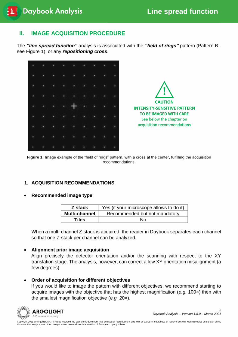
The “line spread function” analysis is associated with the “field of rings” pattern (Pattern B -

see Figure 1), or any repositioning cross.

Figure 1: Image example of the “field of rings” pattern, with a cross at the center, fulfilling the acquisition

recommendations.

1. ACQUISITION RECOMMENDATIONS

• Recommended image type

Z stack Yes (if your microscope allows to do it)

Multi-channel Recommended but not mandatory

Tiles No

When a multi-channel Z-stack is acquired, the reader in Daybook separates each channel

so that one Z-stack per channel can be analyzed.

• Alignment prior image acquisition

Align precisely the detector orientation and/or the scanning with respect to the XY

translation stage. The analysis, however, can correct a low XY orientation misalignment (a

few degrees).

• Order of acquisition for different objectives

If you would like to image the pattern with different objectives, we recommend starting to

acquire images with the objective that has the highest magnification (e.g. 100×) then with

the smallest magnification objective (e.g. 20×).

3




• Signal-to-background ratio (SBR)

Acquire images with enough contrast between the pattern and the background, e.g. a

signal-to-background ratio higher than 2:1.

• Signal-to-noise ratio (SNR)

Acquire images with enough contrast between the pattern and the noise, e.g. a signal-to-

noise ratio higher than 10:1.

• Image intensity

Acquire images within the linear response range of the detector, that is above the detection

limit and below the saturation limit. If available in the acquisition software, use the color-

coded pixels to adjust properly the image intensity. Note that Daybook Analysis cannot

analyze images containing negative values.

• Image dynamic range

When possible, acquire images with a detector that captures raw data with a bit depth of 8

or 16 bits, the allowed image dynamic range for computers (1-byte and 2-byte chunks,

respectively). If the detector captures raw data with a bit depth different from 8 or 16 bits,

convert the images into 8- or 16-bit-dynamic range without losing any information. Note

that if the image file weight is too big for the computational capacity of your computer, the

analysis may not succeed.

• Image sampling rate

The sampling rate of the image should fulfill the Nyquist criterion, i.e. the image pixel size

should be at least the half of the theoretical resolution limit. However, if possible, we

recommend adjusting the image pixel size to one third of the theoretical resolution limit.

2. HOW TO IMAGE THE PATTERN?

1- Find the patterns

a) Start with a low mag objective (such as 10× or 20×). Set the DAPI (405 nm) or GFP (488

nm) channel.

b) Make coincide the center of the slide with respect to the objective.

c) Adjust focus through the eyepieces.

d) Switch to the objective you would like to use. Move the slide to the pattern.

2- Adjust your setup

a) Match the central cross of the pattern with the center of the field of view.

b) Adjust the focus.

4




The best focus usually corresponds to the Z-plane for which the central cross looks the

clearest (qualitative approach) and/or for which the intensity histogram is the broadest

(quantitative approach).

3- Image your pattern

a) Image the pattern by following the acquisition recommendations.

b) Save images into a raw, non-compressed format (for example, the acquisition software proprietary format) or into a lossless compression format (e.g. TIFF). The image file must have a dynamic range of 8 or 16 bits.

5




III. IMAGE ANALYSIS PROCEDURE

1. HOW TO LAUNCH AN ANALYSIS?

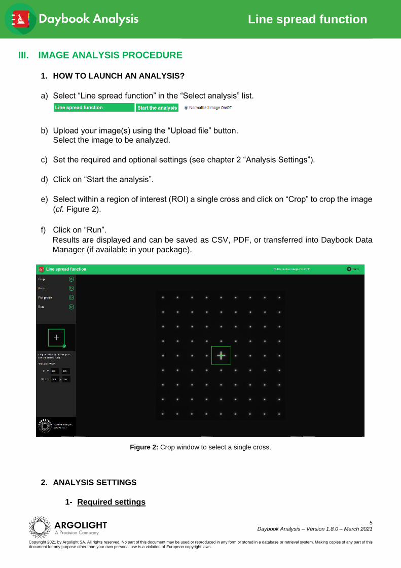
a) Select “Line spread function” in the “Select analysis” list.

b) Upload your image(s) using the “Upload file” button. Select the image to be analyzed.

c) Set the required and optional settings (see chapter 2 “Analysis Settings”).

d) Click on “Start the analysis”.

e) Select within a region of interest (ROI) a single cross and click on “Crop” to crop the image

(cf. Figure 2).

f) Click on “Run”.

Results are displayed and can be saved as CSV, PDF, or transferred into Daybook Data

Manager (if available in your package).

Figure 2: Crop window to select a single cross.

2. ANALYSIS SETTINGS

1- Required settings

6




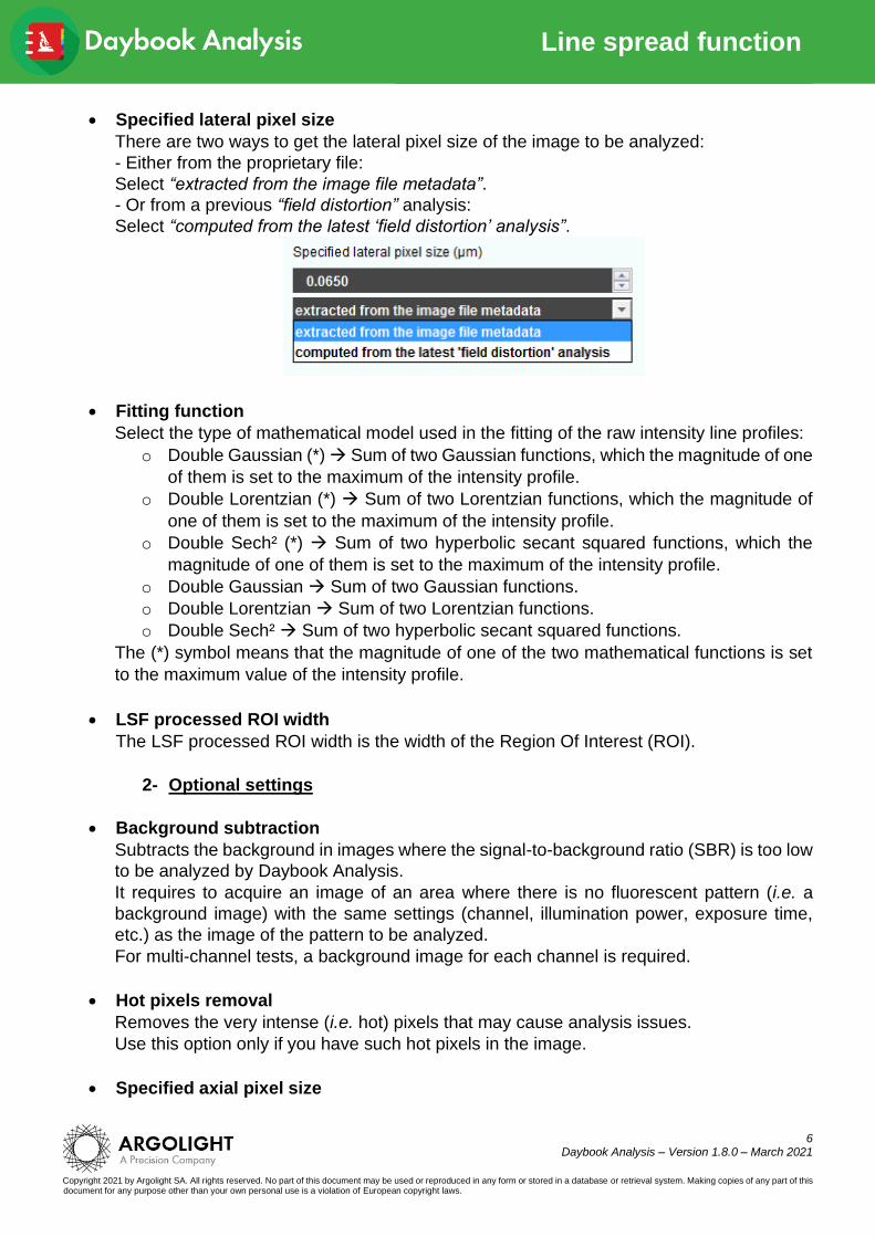
• Specified lateral pixel size

There are two ways to get the lateral pixel size of the image to be analyzed:

- Either from the proprietary file:

Select “extracted from the image file metadata”.

- Or from a previous “field distortion” analysis:

Select “computed from the latest ‘field distortion’ analysis”.

• Fitting function

Select the type of mathematical model used in the fitting of the raw intensity line profiles:

o Double Gaussian (*) → Sum of two Gaussian functions, which the magnitude of one

of them is set to the maximum of the intensity profile.

o Double Lorentzian (*) → Sum of two Lorentzian functions, which the magnitude of

one of them is set to the maximum of the intensity profile.

o Double Sech² (*) → Sum of two hyperbolic secant squared functions, which the

magnitude of one of them is set to the maximum of the intensity profile.

o Double Gaussian → Sum of two Gaussian functions.

o Double Lorentzian → Sum of two Lorentzian functions.

o Double Sech² → Sum of two hyperbolic secant squared functions.

The (*) symbol means that the magnitude of one of the two mathematical functions is set

to the maximum value of the intensity profile.

• LSF processed ROI width

The LSF processed ROI width is the width of the Region Of Interest (ROI).

2- Optional settings

• Background subtraction

Subtracts the background in images where the signal-to-background ratio (SBR) is too low

to be analyzed by Daybook Analysis.

It requires to acquire an image of an area where there is no fluorescent pattern (i.e. a

background image) with the same settings (channel, illumination power, exposure time,

etc.) as the image of the pattern to be analyzed.

For multi-channel tests, a background image for each channel is required.

• Hot pixels removal

Removes the very intense (i.e. hot) pixels that may cause analysis issues.

Use this option only if you have such hot pixels in the image.

• Specified axial pixel size

7




On Z-stacks analysis, the axial pixel size is determined from the proprietary file.

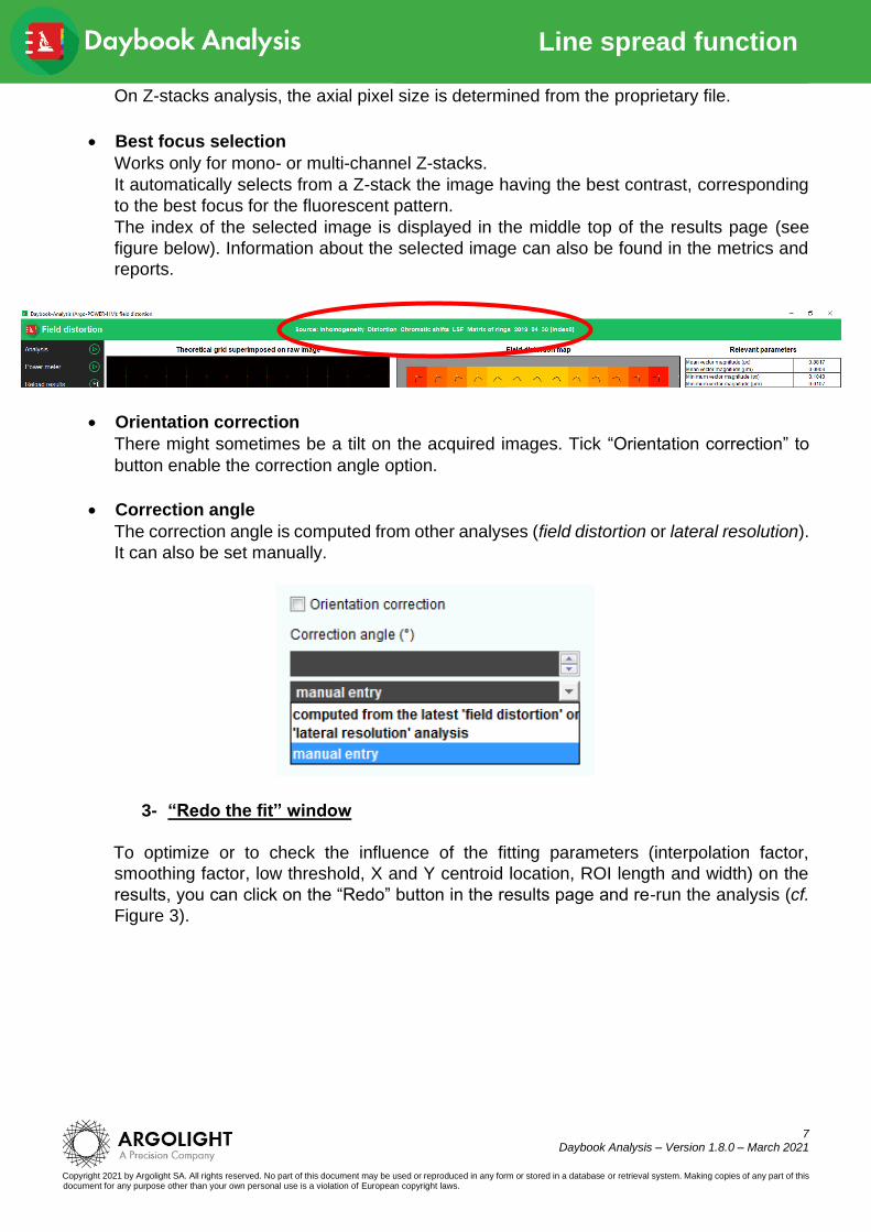
• Best focus selection

Works only for mono- or multi-channel Z-stacks.

It automatically selects from a Z-stack the image having the best contrast, corresponding

to the best focus for the fluorescent pattern.

The index of the selected image is displayed in the middle top of the results page (see

figure below). Information about the selected image can also be found in the metrics and

reports.

• Orientation correction

There might sometimes be a tilt on the acquired images. Tick “Orientation correction” to

button enable the correction angle option.

• Correction angle

The correction angle is computed from other analyses (field distortion or lateral resolution).

It can also be set manually.

3- “Redo the fit” window

To optimize or to check the influence of the fitting parameters (interpolation factor,

smoothing factor, low threshold, X and Y centroid location, ROI length and width) on the

results, you can click on the “Redo” button in the results page and re-run the analysis (cf.

Figure 3).

8




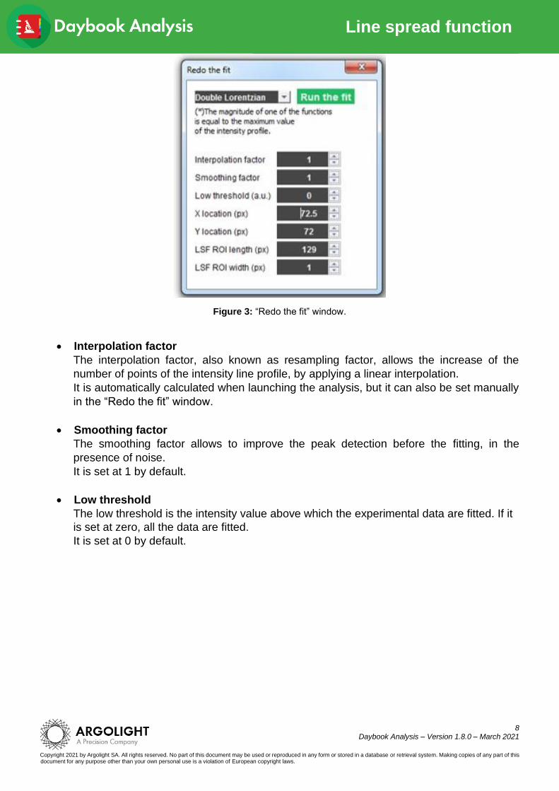
Figure 3: “Redo the fit” window.

• Interpolation factor

The interpolation factor, also known as resampling factor, allows the increase of the

number of points of the intensity line profile, by applying a linear interpolation.

It is automatically calculated when launching the analysis, but it can also be set manually

in the “Redo the fit” window.

• Smoothing factor

The smoothing factor allows to improve the peak detection before the fitting, in the

presence of noise.

It is set at 1 by default.

• Low threshold

The low threshold is the intensity value above which the experimental data are fitted. If it

is set at zero, all the data are fitted.

It is set at 0 by default.

9




IV. RESULTS PAGE DESCRIPTION

1. INTERFACE

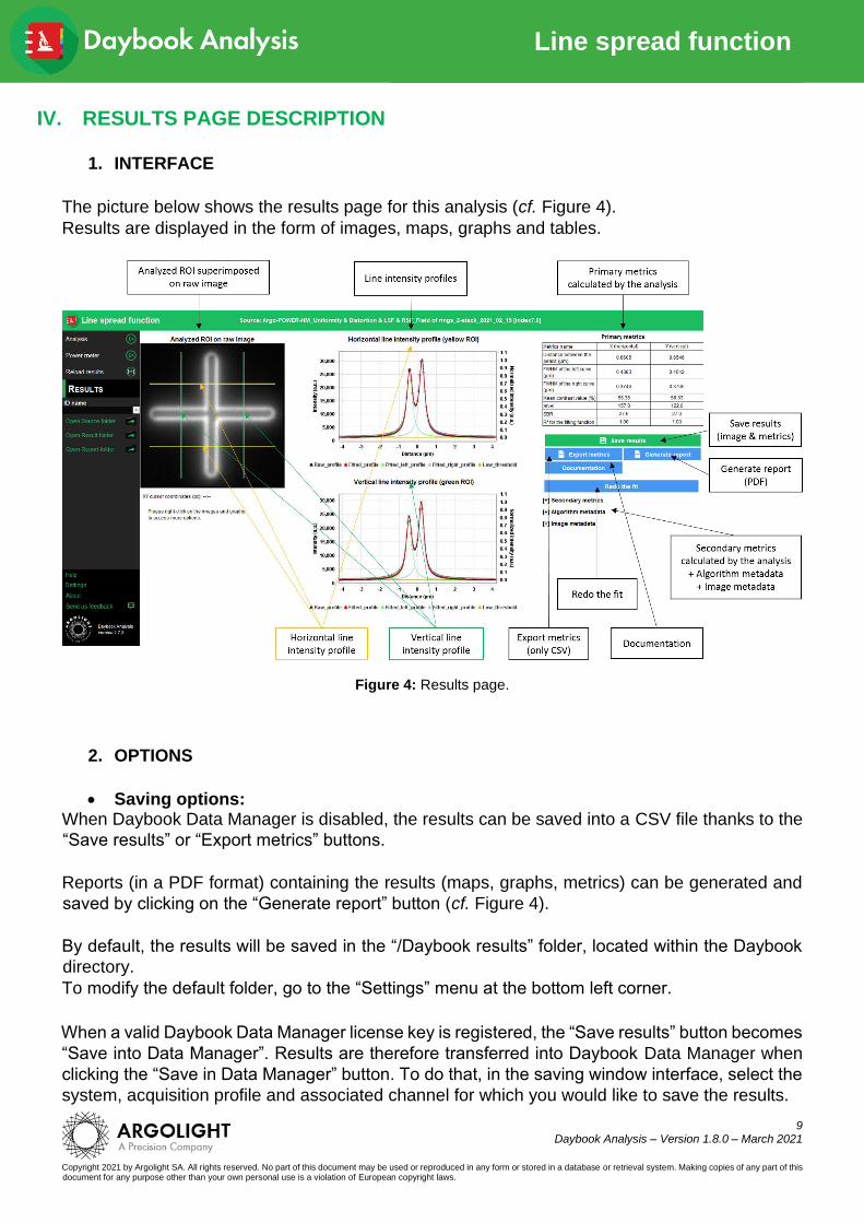
The picture below shows the results page for this analysis (cf. Figure 4).

Results are displayed in the form of images, maps, graphs and tables.

Figure 4: Results page.

2. OPTIONS

• Saving options: When Daybook Data Manager is disabled, the results can be saved into a CSV file thanks to the

“Save results” or “Export metrics” buttons.

Reports (in a PDF format) containing the results (maps, graphs, metrics) can be generated and

saved by clicking on the “Generate report” button (cf. Figure 4).

By default, the results will be saved in the “/Daybook results” folder, located within the Daybook

directory.

To modify the default folder, go to the “Settings” menu at the bottom left corner.

When a valid Daybook Data Manager license key is registered, the “Save results” button becomes

“Save into Data Manager”. Results are therefore transferred into Daybook Data Manager when

clicking the “Save in Data Manager” button. To do that, in the saving window interface, select the

system, acquisition profile and associated channel for which you would like to save the results.

10




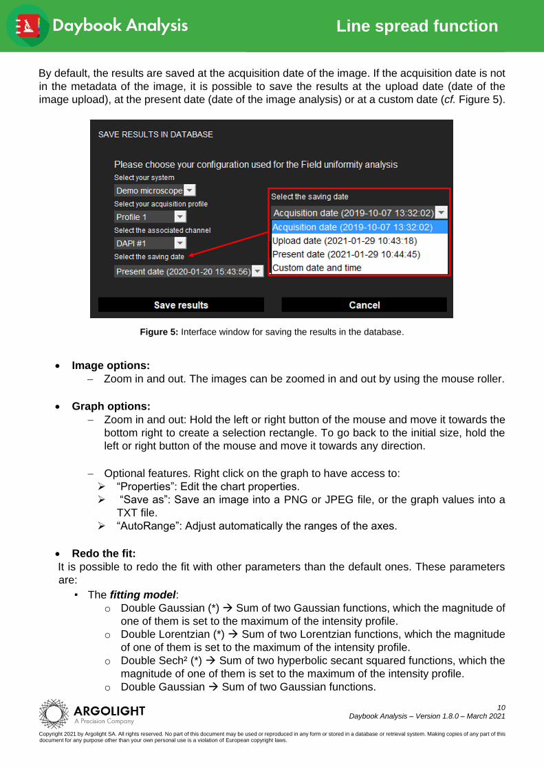
By default, the results are saved at the acquisition date of the image. If the acquisition date is not

in the metadata of the image, it is possible to save the results at the upload date (date of the

image upload), at the present date (date of the image analysis) or at a custom date (cf. Figure 5).

Figure 5: Interface window for saving the results in the database.

• Image options:

− Zoom in and out. The images can be zoomed in and out by using the mouse roller.

• Graph options:

− Zoom in and out: Hold the left or right button of the mouse and move it towards the

bottom right to create a selection rectangle. To go back to the initial size, hold the

left or right button of the mouse and move it towards any direction.

− Optional features. Right click on the graph to have access to:

➢ “Properties”: Edit the chart properties.

➢ “Save as”: Save an image into a PNG or JPEG file, or the graph values into a

TXT file.

➢ “AutoRange”: Adjust automatically the ranges of the axes.

• Redo the fit:

It is possible to redo the fit with other parameters than the default ones. These parameters

are:

▪ The fitting model:

o Double Gaussian (*) → Sum of two Gaussian functions, which the magnitude of

one of them is set to the maximum of the intensity profile.

o Double Lorentzian (*) → Sum of two Lorentzian functions, which the magnitude

of one of them is set to the maximum of the intensity profile.

o Double Sech² (*) → Sum of two hyperbolic secant squared functions, which the

magnitude of one of them is set to the maximum of the intensity profile.

o Double Gaussian → Sum of two Gaussian functions.

11




o Double Lorentzian → Sum of two Lorentzian functions.

o Double Sech² → Sum of two hyperbolic secant squared functions.

The (*) symbol means that the magnitude of one of the two mathematical functions

is set to the maximum value of the intensity profile.

▪ The interpolation factor: change (increase or decrease) the number of values of the

fit, and therefore make it appropriately sampled. The interpolation is linear.

▪ The smoothing factor: in the presence of noise, improve the peak detection before

the fitting.

▪ The low threshold: change the intensity value above which the experimental data are

fitted.

▪ The X and Y locations: change the central locations of the profiles, in the X (horizontal)

and Y (vertical) directions. Use the position indication cursor in the raw image to guess

these values.

▪ The LSF ROI height and width: change the size of the green and yellow regions of

interest (ROI) in the raw image.

12




V. ANALYSIS ALGORITHM DESCRIPTION

1. DIAGRAM

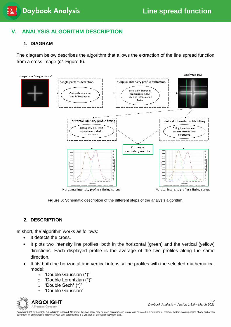
The diagram below describes the algorithm that allows the extraction of the line spread function

from a cross image (cf. Figure 6).

Figure 6: Schematic description of the different steps of the analysis algorithm.

2. DESCRIPTION

In short, the algorithm works as follows:

• It detects the cross.

• It plots two intensity line profiles, both in the horizontal (green) and the vertical (yellow)

directions. Each displayed profile is the average of the two profiles along the same

direction.

• It fits both the horizontal and vertical intensity line profiles with the selected mathematical model:

o “Double Gaussian (*)” o “Double Lorentzian (*)” o “Double Sech² (*)” o “Double Gaussian”

13




o “Double Lorentzian” o “Double Sech²” The (*) symbol means that the magnitude of one of the two mathematical functions is set to the maximum value of the intensity profile.

• It displays the raw intensity line profiles and the fitting functions into two graphs.

See below a description of the different mathematical models used to fit the intensity line profiles.

The same equations are used for the Y and Z directions, with 𝒙 switched for 𝒚 and 𝒛, respectively.

Double Gaussian:

𝐼(𝑥) = 𝐼𝑜𝑓𝑓𝑠𝑒𝑡 + 𝐼1 𝑒𝑥𝑝 [−4 𝑙𝑛(2) (𝑥 − 𝑥1

𝐹𝑊𝐻𝑀𝑥_1)

2

] + 𝐼2 𝑒𝑥𝑝 [−4 𝑙𝑛(2) (𝑥 − 𝑥2

𝐹𝑊𝐻𝑀𝑥_2)

2

]

Double Lorentzian:

𝐼(𝑥) = 𝐼𝑜𝑓𝑓𝑠𝑒𝑡 + 𝐼1

1

1 + (𝑥 − 𝑥1

0.5 𝐹𝑊𝐻𝑀𝑥_1)

2 + 𝐼2

1

1 + (𝑥 − 𝑥2

0.5 𝐹𝑊𝐻𝑀𝑥_2)

2

Double Sech²:

𝐼(𝑥) = 𝐼𝑜𝑓𝑓𝑠𝑒𝑡 + 𝐼1 𝑠𝑒𝑐ℎ2 [2 𝑎𝑟𝑐𝑐𝑜𝑠ℎ(√2) (𝑥 − 𝑥1)

𝐹𝑊𝐻𝑀𝑥_1] + 𝐼2 𝑠𝑒𝑐ℎ2 [

2 𝑎𝑟𝑐𝑐𝑜𝑠ℎ(√2) (𝑥 − 𝑥2)

𝐹𝑊𝐻𝑀𝑥_2]

The following parameters are set as free:

𝐼𝒐𝒇𝒇𝒔𝒆𝒕: offset value.

𝐼𝟏: magnitude of the left curve’s peak.

𝐼𝟐: magnitude of the right curve’s peak.

𝑥1: position of the left curve’s peak.

𝑥2: position of the right curve’s peak.

𝐹𝑊𝐻𝑀𝑥_1: full width at half-maximum of the left curve.

𝐹𝑊𝐻𝑀𝑥_2: full width at half-maximum of the right curve.

14




VI. OUTPUT METRIC DESCRIPTION

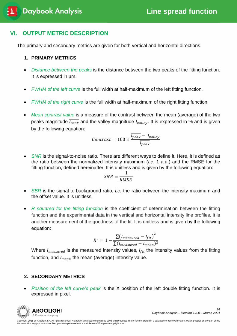
The primary and secondary metrics are given for both vertical and horizontal directions.

1. PRIMARY METRICS

• Distance between the peaks is the distance between the two peaks of the fitting function.

It is expressed in µm.

• FWHM of the left curve is the full width at half-maximum of the left fitting function.

• FWHM of the right curve is the full width at half-maximum of the right fitting function.

• Mean contrast value is a measure of the contrast between the mean (average) of the two

peaks magnitude 𝐼𝑝𝑒𝑎𝑘̅̅ ̅̅ ̅̅ and the valley magnitude 𝐼𝑣𝑎𝑙𝑙𝑒𝑦. It is expressed in % and is given

by the following equation:

𝐶𝑜𝑛𝑡𝑟𝑎𝑠𝑡 = 100 ×𝐼𝑝𝑒𝑎𝑘̅̅ ̅̅ ̅̅ − 𝐼𝑣𝑎𝑙𝑙𝑒𝑦

𝐼𝑝𝑒𝑎𝑘̅̅ ̅̅ ̅̅

• SNR is the signal-to-noise ratio. There are different ways to define it. Here, it is defined as

the ratio between the normalized intensity maximum (i.e. 1 a.u.) and the RMSE for the

fitting function, defined hereinafter. It is unitless and is given by the following equation:

𝑆𝑁𝑅 =1

𝑅𝑀𝑆𝐸

• SBR is the signal-to-background ratio, i.e. the ratio between the intensity maximum and

the offset value. It is unitless.

• R squared for the fitting function is the coefficient of determination between the fitting

function and the experimental data in the vertical and horizontal intensity line profiles. It is

another measurement of the goodness of the fit. It is unitless and is given by the following

equation:

𝑅2 = 1 −∑(𝐼𝑚𝑒𝑎𝑠𝑢𝑟𝑒𝑑 − 𝐼𝑓𝑖𝑡)

2

∑(𝐼𝑚𝑒𝑎𝑠𝑢𝑟𝑒𝑑 − 𝐼𝑚𝑒𝑎𝑛)2

Where 𝐼𝑚𝑒𝑎𝑠𝑢𝑟𝑒𝑑 is the measured intensity values, 𝐼𝑓𝑖𝑡 the intensity values from the fitting

function, and 𝐼𝑚𝑒𝑎𝑛 the mean (average) intensity value.

2. SECONDARY METRICS

• Position of the left curve’s peak is the X position of the left double fitting function. It is expressed in pixel.

15




• Position of the right curve’s peak is the X position of the right double fitting function. It is expressed in pixel.

• Magnitude of the left curve’s peak is the magnitude of the left fitting function. It is expressed in arbitrary unit.

• Magnitude of the right curve’s peak is the magnitude of the right fitting function. It is expressed in arbitrary unit.

• Offset value is the offset value used for the fitting. It is expressed in arbitrary unit.

• Intensity maximum is the maximum intensity in the raw image. It is expressed in arbitrary

unit.

• Intensity minimum is the minimum intensity in the raw image. It is expressed in arbitrary

unit.

• RMSE for the fitting function is the root mean square error between the fitting function and

the experimental data in the vertical and horizontal intensity line profiles. It is a

measurement of the goodness of the fit. It is expressed in arbitrary unit and is given by the

following equation:

𝑅𝑀𝑆𝐸 = √1

𝑛∑(𝐼𝑚𝑒𝑎𝑠𝑢𝑟𝑒𝑑 − 𝐼𝑓𝑖𝑡)

2

Where n is the number of experimental points, 𝐼𝑚𝑒𝑎𝑠𝑢𝑟𝑒𝑑 the measured intensity values and

𝐼𝑓𝑖𝑡 the intensity values from the fitting function.

3. ALGORITHM METADATA

• Analysis date is the date at which the analysis has been performed.

• Software version is the version of the software.

• Product type is the type of Argolight product selected in the panel settings.

• Angle value used for the orientation correction is the angle value applied to the analyzed image to correct a small rotation/tilt of the pattern, usually due to camera or laser scanning misalignment in microscopes. This angle value can either be automatically calculated by some of the algorithms and/or previously set in the analysis settings. It is expressed in degree.

• Background subtraction indicates if the “Background subtraction” option has been

activated or not.

16




• Hot pixels removal indicates if the “Hot pixels removal” option has been activated or not.

• Best focus selection indicates if the “Best focus selection” option has been activated or

not.

• Index of the selected image in the stack indicates the index of the image in the stack that

has been selected when activating the “Best focus selection” option.

• Fitting model type is the type of mathematical model used in the fitting of the raw intensity line profiles: “Double Gaussian (*)”, “Double Lorentzian (*)”, “Double Sech² (*)”, “Double Gaussian” , “Double Lorentzian”, or “Double Sech²”. The (*) symbol means that the magnitude of one of the two mathematical functions is set to the maximum value of the intensity profile.

• Interpolation factor is the factor used to linearly interpolate the horizontal and vertical intensity line profiles. It is unitless, and automatically calculated according to the following formula:

𝐼𝑛𝑡𝑒𝑟𝑝𝑜𝑙𝑎𝑡𝑖𝑜𝑛 𝑓𝑎𝑐𝑡𝑜𝑟 = Round up {1200 (𝑛𝑢𝑚𝑏𝑒𝑟 𝑜𝑓 𝑓𝑖𝑡𝑡𝑖𝑛𝑔 𝑝𝑜𝑖𝑛𝑡𝑠 ; 𝑝𝑥)

𝑅𝑆𝐹 𝑅𝑂𝐼 𝑙𝑒𝑛𝑔𝑡ℎ (𝑝𝑥)}

It can also be set manually in the “Redo the fit” window.

• Interpolation factor is the factor set to interpolate linearly the horizontal and vertical intensity line profiles. It is unitless.

• Smoothing factor is the factor set to smooth the horizontal and vertical intensity line profiles. It is unitless.

• Low threshold is the threshold below which the raw data are not fitted. It is expressed in arbitrary unit.

• LSF ROI length is the length set for the region of interest within the “cross” pattern. It is expressed in pixel.

• LSF ROI width is the width set for the region of interest within the “cross” pattern. It is expressed in pixel.

• X coordinate of the ROI is the coordinate along X (starting from the top left corner) of the

cropped area in the image. A null value corresponds to an uncropped image. It is

expressed in pixel.

• Y coordinate of the ROI is the coordinate along Y (starting from the top left corner) of the

cropped area in the image. A null value corresponds to an uncropped image. It is

expressed in pixel.

• ROI width is the width of the cropped area in the image. A value equal to the image width

corresponds to an uncropped image. It is expressed in pixel.

17




• ROI height is the height of the cropped area in the image. A value equal to the image height

corresponds to an uncropped image. It is expressed in pixel.

4. IMAGE METADATA

• Acquisition date is the date at which the acquisition of the image has been performed. If

this information is not contained in the metadata of the image, then the note “unknown” is

displayed.

• Specified lateral pixel size is the size of one pixel, provided by the metadata associated to the raw image. It is expressed in µm.

• Specified axial pixel size is the interval between each slice of the stack, provided by the metadata associated to the raw image. It is expressed in µm.

• Image dynamic range is the dynamic range of the image, provided by the metadata

associated to the raw image. It is expressed in bits (8 or 16 bits).

• Detector bit depth is the data capturing range of the detector, provided by the metadata

associated to the raw image. It is expressed in bits. For example, a 16-bit detector can

capture 216 = 65536 intensity levels.

• Image width is the width of the image, provided by the metadata associated to the raw

image. It is expressed in pixel.

• Image height is the height of the image, provided by the metadata associated to the raw

image. It is expressed in pixel.

18




Encountered an issue or a question when using Daybook Analysis?

Please send a screenshot and your issue description at:

[email protected]

mailto:[email protected]

Documents

Line spread function - Argolight