Embed Size (px)
Citation preview
ORE Open Research Exeter
TITLE
Line and continuum radiative transfer modelling of AA Tau
AUTHORS
Esau, Claire F.; Harries, Tim J.; Bouvier, Jerome
JOURNAL
Monthly Notices of the Royal Astronomical Society
DEPOSITED IN ORE
14 April 2015
This version available at
http://hdl.handle.net/10871/16793
COPYRIGHT AND REUSE
Open Research Exeter makes this work available in accordance with publisher policies.
A NOTE ON VERSIONS
The version presented here may differ from the published version. If citing, you are advised to consult the published version for pagination, volume/issue and date ofpublication
MNRAS 443, 1022–1043 (2014) doi:10.1093/mnras/stu1211
Line and continuum radiative transfer modelling of AA Tau
Claire F. Esau,1‹ Tim J. Harries1 and Jerome Bouvier2
1School of Physics, University of Exeter, Stocker Road, Exeter EX4 4QL, UK2UJF-Grenoble 1/CNRS-INSU, Institut de Planetologie et d’Astrophysique de Grenoble (IPAG) UMR 5274, Grenoble F-38041, France
Accepted 2014 June 17. Received 2014 June 15; in original form 2014 May 8
ABSTRACTWe present photometric and spectroscopic models of the Classical T Tauri star AA Tau.Photometric and spectroscopic variability present in observations of AA Tau is attributed toa magnetically induced warp in the accretion disc, periodically occulting the photosphereon an 8.2 d time-scale. Emission line profiles show signatures of both infall, attributed tomagnetospherically accreting material, and outflow. Using the radiative transfer code TORUS,we have investigated the geometry and kinematics of AA Tau’s circumstellar disc and outflow,which is modelled here as a disc wind. Photometric models have been used to constrain theaspect ratio of the disc, the offset angle of the magnetosphere dipole with respect to the stellarrotation axis, and the inner radius of the circumstellar disc. Spectroscopic models have beenused to constrain the wind and magnetosphere temperatures, wind acceleration parameter, andmass-loss rate. We find that observations are best fitted by models with a mass accretion rateof 5 × 10⁻⁹ M� yr−1, a dipole offset of between 10◦ and 20◦, a magnetosphere that truncatesthe disc from 5.2 to 8.8R�, a mass-loss-rate to accretion-rate ratio of ∼0.1, a magnetospheretemperature of 8500–9000 K, and a disc-wind temperature of 8000 K.
Key words: accretion, accretion discs – stars: individual: AA Tau – stars: magnetic field –stars: pre-main-sequence – stars: variables: T Tauri.
1 IN T RO D U C T I O N
Classical T Tauri stars (CTTs) are low-mass pre-main-sequencestars. Spectroscopic studies of CTTs show high-velocity redshiftedabsorption components in their recombination lines, providing ev-idence of accretion from the circumstellar disc (e.g. Edwardset al. 1994; Muzerolle, Calvet & Hartmann 1998). Spectra alsoshow the presence of excess ultraviolet (UV) emission. These canbe explained by a magnetospheric accretion model (Bertout, Basri& Bouvier 1988; Konigl 1991; Hartmann, Hewett & Calvet 1994,and references therein), in which the magnetosphere of a CTT trun-cates the circumstellar disc, at which point material attaches to thefield lines and falls on to the photosphere. The accreting materialtravels ballistically and its kinetic energy is liberated as thermalradiation on impact with the photosphere, producing hotspots nearthe magnetosphere poles. These are the sources of the excess UVemission. Typical accretion rates of CTTs range between 10−7 and10−9 M� yr−1 (e.g. Basri & Bertout 1989).
Spectra of CTTs also show evidence of outflows on differentscales, with blueshifted absorption components and blueshiftedforbidden line emission present at high velocities (Mundt 1984;Edwards et al. 1987). These signatures are thought to be due tostellar winds, disc winds, and jets. Stellar winds are understoodto be powered by a fraction of the energy released at the base of
� E-mail: [email protected]
the accretion streams, causing material to escape along open mag-netic field lines from the stellar surface (e.g. Matt & Pudritz 2005).Disc winds emanate from open field lines threading the accretiondisc (e.g. Camenzind 1990) in a bipolar conical outflow (Konigl &Pudritz 2000). This paradigm was first proposed by Blandford &Payne (1982) to explain observations of jets emanating from theaccretion discs of black holes, and was extended by Pudritz &Norman (1983) to explain bipolar outflows associated with em-bedded protostars. Highly collimated high-velocity jets, emanatingfrom closer to the star than less collimated disc winds, have also beenobserved in association with young stellar objects (e.g. Burrowset al. 1996; Appenzeller, Bertout & Stahl 2005). The correlationbetween mass accretion diagnostics and wind signatures imply thatwinds are powered by the accretion process (Cabrit et al. 1990).Additionally, there is no evidence for mass-loss in the spectraof weak-line T Tauri stars, i.e. when there is no accretion occur-ring. While stellar winds do appear to contribute to mass-loss, discwinds seem to dominate (Cabrit 2007). However, there are numer-ous possible mechanisms for disc-wind formation and the preciseorigin, or the relative contributions from disc winds of different ori-gins, is still debated (see Ferreira, Dougados & Cabrit 2006, for areview).
The magnetospheric accretion paradigm is supported by the re-sults of line models. Hartmann et al. (1994) reproduced observedredshifted absorption components and blueshifted emission peaksof Balmer lines using a simple radiative transfer model of magneto-spheric infall. This model was extended by Muzerolle et al. (1998),
C© 2014 The AuthorsPublished by Oxford University Press on behalf of the Royal Astronomical Society
at Unversity of E
xeter on April 7, 2015
http://mnras.oxfordjournals.org/
Dow
nloaded from
Radiative transfer modelling of AA Tau 1023
replacing the two-level atom approximation with a multilevel hydro-gen atom in statistical equilibrium, followed by a further extension(Muzerolle, Calvet & Hartmann 2001) which included line broaden-ing and sodium line calculations. Muzerolle et al. (2001) presenteda grid of models across a range of parameter space, varying magne-tosphere temperature, line-of-sight inclination, accretion rate, andmagnetosphere size. They found Hα lines which included Starkbroadening were more consistent with observations than previousresults. They also found instances where line profiles peaked nearzero velocity, allowing for natural interpretation of observed CTTspectra that do not show the blueward emission peaks calculatedin previous models. While a number of lines were included in thestudy, Hβ was the focus of a detailed examination of profile shapes.A similar study focusing on Hα was carried out by Kurosawa,Harries & Symington (2006) using the radiative transfer code TORUS.This used the same accretion flow model and broadening mecha-nisms as Muzerolle et al. but the model was extended to includea self-consistent calculation for the hotspot temperature. A discwind was also included using the formalism of Knigge, Woods &Drew (1995; see also Long & Knigge 2002), where a biconical windemerges from a rotating disc. Kurosawa et al. compared results witha classification scheme for Hα lines proposed by Reipurth, Pedrosa& Lago (1996), in which seven classes of line shape were defined de-pending on the relative strength of the secondary peak to the primarypeak (in the case of double-peaked emission lines), and whether thesecondary falls blueward or redward of the primary. While some in-dividual profiles were reproducible using models consisting solelyof either a disc wind or a magnetospheric accretion flow, Kurosawaet al. found that all classes were readily explained using a hybridwind-accretion model by varying the angle of inclination to the lineof sight, the ratio of mass accretion to loss rates, the wind acceler-ation rate, and magnetosphere temperature (although one class wasbetter explained using a bipolar outflow or spherical wind, ratherthan the disc-wind model).
The motivation for this study is to test the observed line formationusing an object which has very well-constrained physical param-eters. AA Tau is an ideal candidate for magnetospheric accretionstudies due to its high inclination angle of 75◦ (Bouvier et al. 1999).It is a typical CTT, with a mass of 0.85 M� and a radius of about1.85 R�. Indeed, there have been many observation campaigns in-volving AA Tau, both photometric and spectroscopic (e.g. Bouvieret al. 1999, 2003, and the All Sky Automated Survey, ASAS, e.g.Pojmanski, Pilecki & Szczygiel 2005). Spectropolarimetric obser-vations have also been used to map the magnetic field of AA Tauat different epochs (Donati et al. 2010). Photometric observationsshow periodic dips in the light curve of AA Tau, which have beenexplained by azimuthally asymmetric accretion. If the magneto-sphere axis is misaligned with the rotation axis, the two hotspotsproduced near the magnetosphere poles will sweep in and out ofview as the star rotates, separated by half a rotation period. Theinner regions of the disc undergo turbulence at the points of interac-tion with the magnetosphere, causing two waves of material to riseup in disc warps on opposite sides of the star (Bouvier et al. 1999).Each warp obscures the photosphere, and since the line-of-sightinclination of AA Tau is sufficiently high, the photosphere andhotspot in the observable hemisphere are only periodically visible.This causes photometric variations, where AA Tau appears fainterduring occultation and brighter when the warp is behind the star.AA Tau’s photometric period has been shown to vary from 8.2 to8.6 d (e.g. Vrba et al. 1989; Bouvier et al. 1999; Artmenko, Grankin& Petrov 2012). This general trend is supported by radial velocitymeasurements yielding a period of 8.29 d (Bouvier et al. 2003),
although observations do show more complex variability occasion-ally, with multiple smaller amplitude dips having been observedby Bouvier et al. (2003) and in Pojmanski et al. (2005), hereafterASAS. Conversely, there have also been occurrences where no orvery little photometric variability has been apparent over a numberof stellar rotation periods. The degree of photometric variability isexpected to change with time as the geometry of the system itselfwill not remain uniform – the size of the disc warp will vary as thefield lines break and reconnect, with short-term variations betweenrotations due to changes in the local density of material. Photo-metric variations have been found to reach an amplitude of �V ∼1.7 mag. Since the photometric period is generally similar to therotational period of AA Tau, a constraint is placed on the position ofthe inner edge of the disc, which is equal to the Keplerian corotationradius of 8.8R� for an 8.22 d period. While initially AA Tau’s pho-tometric behaviour was regarded as atypical of CTT photometry,light curves showing ‘AA Tau-like’ variations – that is, variationsdue to an occulting wall, rather than more periodic variations dueto solely the hotspot or completely irregular variations – have beenobserved in ∼28 per cent of CTTs (Alencar et al. 2010), from a sam-ple of 83 CTTs. AA Tau is a particularly well-constrained objectgeometrically and shows signatures of azimuthally varying accre-tion and outflow, both photometrically and spectroscopically, whichare consistent with the paradigm of magnetospheric accretion. Weare therefore able to use this star-disc-wind system to strongly testthe paradigm of magnetospheric accretion in relation to CTTs ingeneral.
Observational photometry from Bouvier et al. (1999, 2003, 2007,hereafter B99, B03, and B07, respectively) and ASAS is presentedin Section 2, followed by a description of the model calculationsand an analysis of the results. Observational spectroscopy fromB07 is presented in Section 3, followed by a description of theradiative transfer code TORUS. Synthetic Hα, Hβ, and Hγ spectrafor AA Tau are presented, followed by an analysis of the results. Theimplications of these results are discussed in Section 4, followed bya summary in Section 5.
2 PH OTO M E T RY
The aim here is to use a self-consistent geometrical model of amagnetosphere and an optically thick disc warp to produce syntheticlight curves of AA Tau. Models were run using the radiative transfercode TORUS (Harries 2000; Symington, Harries & Kurosawa 2005).Various synthetic light curves were produced by varying numerousparameters and the resulting data was compared with photometricobservations in order to find the parameter set most consistent withobservations. It is well known that occultation events come andgo, with epoch to epoch variations observed across occultations,so we collated as much photometric data as was publicly availableto compare with the resulting synthetic light curves. We cannotexpect a single parameter set to consistently fit all epochs since themagnetic field of AA Tau varies azimuthally, causing the height ofthe warp (and hence the depth of the occultation) to vary over time.We are therefore looking for a model which is broadly consistentwith the typical deep occultation events observed to occur over an8.22 d period.
2.1 Observational photometry
B- and V-band photometric data from B99 were obtained in 1995November and December, data from B03 were obtained between1999 August and 2000 January, and data from B07 were obtained
MNRAS 443, 1022–1043 (2014)
at Unversity of E
xeter on April 7, 2015
http://mnras.oxfordjournals.org/
Dow
nloaded from
1024 C. F. Esau, T. J. Harries and J. Bouvier
Table 1. Sources of photometric data and the amount of data obtained ineach case.
Source Filter Dates of observations No. of data points
Bouvier et al. (1999) 11-11-95 – 11-12-95 262 (B), 275 (V)Bouvier et al. (2003) BV 09-08-99 – 05-01-00 250 (B), 273 (V)Bouvier et al. (2007) 11-09-04 – 25-01-05 99 (B), 115 (V)
13-12-02 – 13-03-03 5510-08-03 – 24-02-04 6421-09-04 – 19-12-04 101
Pojmanski et al. V 17-08-05 – 02-01-06 44(2005) 20-08-07 – 06-03-08 48
13-09-08 – 28-02-09 3614-09-09 – 27-11-09 10
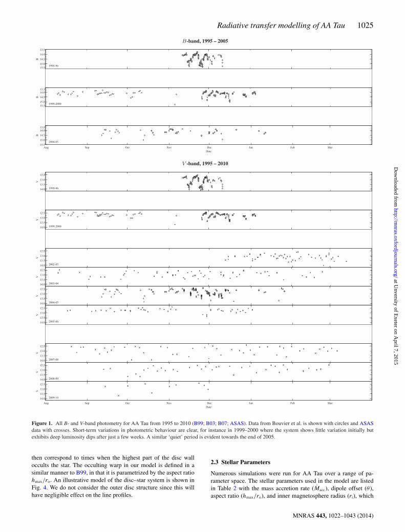
between 2004 September and 2005 January. Additional V-banddata from ASAS were obtained between 2002 December and 2009November. These have been split into seven epochs for the pho-tometric analysis, as shown in Table 1. While a number of theseepochs do not have sufficient data for a detailed study on varia-tions in the structure of AA Tau over individual rotations, they arestill useful in determining the average nature of AA Tau’s varyingstructure over time. All data are plotted in Fig. 1, demonstratingthe long-term variation in photometry. One clear source of variationbetween data sets is the photometric amplitude. B99 data show aphotometric amplitude of about 1.6 mag in V, which decreases toabout 1.0 mag in B03 and B07 (although B03 shows two luminositydips per period, and one instance where a dip disappeared in onecycle). It is obvious from Fig. 1 that the data from the first por-tion of the 1999 observing campaign does not produce well-definedphotometric modulation, with variations of about 0.6 mag over anumber of weeks. A similar ‘quiet’ spell occurs in 2005–2006, witheven less photometric variation. Conversely, data from 2007 to 2008show variations returning to about �V = 1.5 mag.
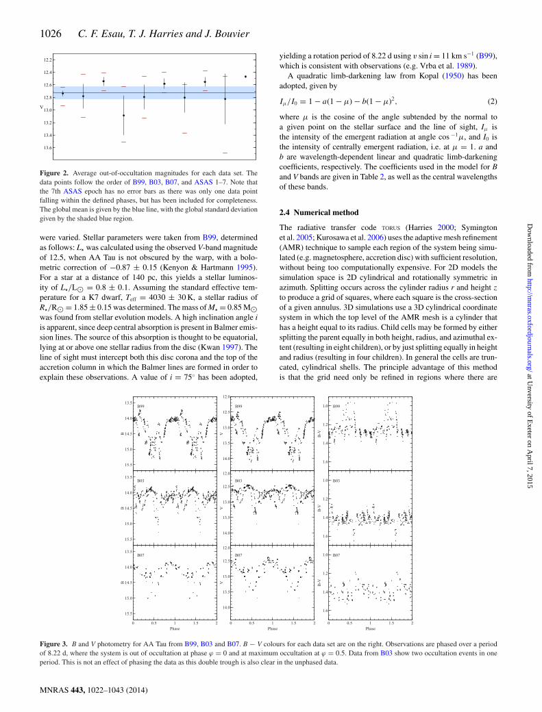
In addition to variations in amplitude, AA Tau also exhibits vari-ations in brightness. Fig. 2 shows the average out-of-occultationV-band magnitudes for each data set. Each set of observational datawas phased, where phase ϕ = 0 is out of occultation and ϕ = 0.5is during occultation. The mean magnitude was calculated for datawith ϕ < 0.1 and ϕ > 0.9 to find an average out-of-occultationmagnitude during each epoch, along with the standard deviation ofeach data set. The global mean and standard deviation are given bythe blue line and light blue shaded region, respectively. The globalmean lies at V = 12.73, while the full spread in data varies from amaximum brightness of V = 12.37 (ASAS 5) to a minimum bright-ness of V = 13.70 (ASAS 6). The range in individual data sets isdenoted by red dashes.
Colour changes are evident in AA Tau’s photometry, with theaverage (B − V) colour increasing from ∼1.25 in 1995 to ∼1.42 in1999 (B03). This reddening has been attributed to a lower accretionrate in 1999, causing a reduction in the blue excess. The average(B−V) colour remained in the region of 1.4 in the 2004 observa-tions, although there is more dispersion. In each case, the variationsin colour are significantly less than the variations in brightness,with colour variations of about 0.4 mag in 1995 compared to abrightness decrease of about 1.6 mag in B and V. Colour variationsdecreased to about 0.3 mag in 1999 and 2004, with photometricamplitudes of about 1.0 mag in each case. Phased colour plots arepresented in Fig. 3, along with phased B and V observations. Whilethe 1995 colour plot appears to show the system being bluer whenfainter, there is no evidence of a correlation between colour and
brightness in later observations. As pointed out by B07, the bluestand reddest colours in the 2004 data both occur during brightnessminimum.
Recently AA Tau’s photometry has changed significantly, witha decrease in the average brightness level by ∼2 mag occurringduring 2011 (Bouvier et al. 2013). Observations taken in 2011show no evidence of coherent photometric modulations, but by theend of 2012 an 8.2 d period is recovered (while remaining faint).V-band magnitudes during this period range from V � 14 to 16.5,with an average brightness of V � 14.8 and an amplitude of up to0.9 mag. This has been attributed to a density perturbation in thedisc, resulting in an increase in visual extinction from Av = 0.8 mag(B99) to Av ≥ 4 mag with no evidence for any significant change inthe mass accretion rate.
2.2 Geometry
The magnetosphere of AA Tau is modelled as a dipole field alongwhich we assume circumstellar material to be travelling ballistically.This flow is defined by the mass accretion rate Macc, stellar mass M�,stellar radius R�, dipole offset θ , and inner and outer magnetosphereradii, ri and ro, respectively. The dipole offset is the angle by whichthe dipole is tilted with respect to the axis of rotation, where θ = 0◦
describes a system in which the magnetic field and stellar rotationaxis are aligned. The system is also inclined to the observer by anangle i. The effects that i and θ have on the observed photometricvariations of T Tauri stars have been studied in detail by Mahdavi& Kenyon (1998). They also discuss the most likely path that ac-creting material will take. A tilted dipole results in some field linesproviding a longer path to the stellar surface than others. Materialin the accretion disc will therefore need to travel further along somelines than others. Material travelling along the longer lines needs togain potential energy in climbing the line, whereas material travel-ling from the same position in the disc but over the opposite, shorterfield line is able to simply fall on to the star. Surface hotspots aredefined geometrically where the flow hits the stellar surface. We as-sume that all the kinetic energy from the accretion flow is liberatedas thermal radiation. The temperature of these hotspots is calculatedfrom the accretion luminosity and the area of the hotspots. Typically,we have found that the hotspots cover about 2 per cent of the stellarsurface.
Material is assumed to accrete from around the corotation ra-dius, interior to which the disc is truncated by the magnetic field.ri and ro define the inner and outer radii at which closed mag-netic field lines transport material from the disc to the star. In themodels presented here, material is assumed to accrete only alongenergetically favourable field lines, resulting in an azimuthal vari-ation in accretion spot luminosity. The resulting shocks from ma-terial hitting the stellar surface produce an accretion signature inthe form of a thin elliptical arc near the magnetic pole in eachhemisphere.
The photometric variations of AA Tau have been attributed to awarp in the circumstellar disc (B99), caused by the tilt of the mag-netic dipole. This produces an optically thick occulting wall. Thewall height of the inner disc has been modelled as an azimuthallyvarying cosine function by B99,
h(φ) = hmax
∣∣∣∣cosπ (φ − φ0)
2
∣∣∣∣ , (1)
where h is the height of the disc at azimuth angle φ and φ0 is theazimuth at which the disc is at its highest, hmax. This relation hasbeen shown roughly to fit observations. The photometric minima
MNRAS 443, 1022–1043 (2014)
at Unversity of E
xeter on April 7, 2015
http://mnras.oxfordjournals.org/
Dow
nloaded from
Radiative transfer modelling of AA Tau 1025
Figure 1. All B- and V-band photometry for AA Tau from 1995 to 2010 (B99; B03; B07; ASAS). Data from Bouvier et al. is shown with circles and ASASdata with crosses. Short-term variations in photometric behaviour are clear, for instance in 1999–2000 where the system shows little variation initially butexhibits deep luminosity dips after just a few weeks. A similar ‘quiet’ period is evident towards the end of 2005.
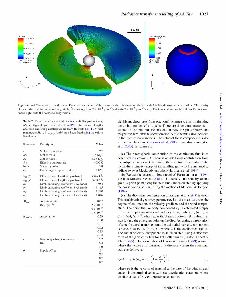
then correspond to times when the highest part of the disc walloccults the star. The occulting warp in our model is defined in asimilar manner to B99, in that it is parametrized by the aspect ratiohmax/ro. An illustrative model of the disc–star system is shown inFig. 4. We do not consider the outer disc structure since this willhave negligible effect on the line profiles.
2.3 Stellar Parameters
Numerous simulations were run for AA Tau over a range of pa-rameter space. The stellar parameters used in the model are listedin Table 2 with the mass accretion rate (Macc), dipole offset (θ ),aspect ratio (hmax/ro), and inner magnetosphere radius (ri), which
MNRAS 443, 1022–1043 (2014)
at Unversity of E
xeter on April 7, 2015
http://mnras.oxfordjournals.org/
Dow
nloaded from
1026 C. F. Esau, T. J. Harries and J. Bouvier
Figure 2. Average out-of-occultation magnitudes for each data set. Thedata points follow the order of B99, B03, B07, and ASAS 1–7. Note thatthe 7th ASAS epoch has no error bars as there was only one data pointfalling within the defined phases, but has been included for completeness.The global mean is given by the blue line, with the global standard deviationgiven by the shaded blue region.
were varied. Stellar parameters were taken from B99, determinedas follows: L� was calculated using the observed V-band magnitudeof 12.5, when AA Tau is not obscured by the warp, with a bolo-metric correction of −0.87 ± 0.15 (Kenyon & Hartmann 1995).For a star at a distance of 140 pc, this yields a stellar luminos-ity of L�/L� = 0.8 ± 0.1. Assuming the standard effective tem-perature for a K7 dwarf, Teff = 4030 ± 30 K, a stellar radius ofR�/R� = 1.85 ± 0.15 was determined. The mass of M� = 0.85 M�was found from stellar evolution models. A high inclination angle iis apparent, since deep central absorption is present in Balmer emis-sion lines. The source of this absorption is thought to be equatorial,lying at or above one stellar radius from the disc (Kwan 1997). Theline of sight must intercept both this disc corona and the top of theaccretion column in which the Balmer lines are formed in order toexplain these observations. A value of i = 75◦ has been adopted,
yielding a rotation period of 8.22 d using v sin i = 11 km s−1 (B99),which is consistent with observations (e.g. Vrba et al. 1989).
A quadratic limb-darkening law from Kopal (1950) has beenadopted, given by
Iμ/I0 = 1 − a(1 − μ) − b(1 − μ)2, (2)
where μ is the cosine of the angle subtended by the normal toa given point on the stellar surface and the line of sight, Iμ isthe intensity of the emergent radiation at angle cos −1μ, and I0 isthe intensity of centrally emergent radiation, i.e. at μ = 1. a andb are wavelength-dependent linear and quadratic limb-darkeningcoefficients, respectively. The coefficients used in the model for Band V bands are given in Table 2, as well as the central wavelengthsof these bands.
2.4 Numerical method
The radiative transfer code TORUS (Harries 2000; Symingtonet al. 2005; Kurosawa et al. 2006) uses the adaptive mesh refinement(AMR) technique to sample each region of the system being simu-lated (e.g. magnetosphere, accretion disc) with sufficient resolution,without being too computationally expensive. For 2D models thesimulation space is 2D cylindrical and rotationally symmetric inazimuth. Splitting occurs across the cylinder radius r and height z
to produce a grid of squares, where each square is the cross-sectionof a given annulus. 3D simulations use a 3D cylindrical coordinatesystem in which the top level of the AMR mesh is a cylinder thathas a height equal to its radius. Child cells may be formed by eithersplitting the parent equally in both height, radius, and azimuthal ex-tent (resulting in eight children), or by just splitting equally in heightand radius (resulting in four children). In general the cells are trun-cated, cylindrical shells. The principle advantage of this methodis that the grid need only be refined in regions where there are
Figure 3. B and V photometry for AA Tau from B99, B03 and B07. B − V colours for each data set are on the right. Observations are phased over a periodof 8.22 d, where the system is out of occultation at phase ϕ = 0 and at maximum occultation at ϕ = 0.5. Data from B03 show two occultation events in oneperiod. This is not an effect of phasing the data as this double trough is also clear in the unphased data.
MNRAS 443, 1022–1043 (2014)
at Unversity of E
xeter on April 7, 2015
http://mnras.oxfordjournals.org/
Dow
nloaded from
Radiative transfer modelling of AA Tau 1027
Figure 4. AA Tau, modelled with TORUS. The density structure of the magnetosphere is shown on the left with AA Tau shown centrally in white. The densityof material covers two orders of magnitude, Eincreasing from 2 × 10¹⁴ g cm−3 (blue) to 2 × 10¹² g cm−3 (red). The temperature structure of AA Tau is shownon the right, with the hotspot clearly visible.
Table 2. Parameters for our grid of models. Stellar parameters i,M�, R�, Teff and ro are fixed, taken from B99. Effective wavelengthsand limb-darkening coefficients are from Howarth (2011). Modelparameters Macc, hmax/ro,ri and θ have been fitted using the valueslisted here.
Parameter Description Value
i Stellar inclination 75◦M� Stellar mass 0.8 M�R� Stellar radius 1.85 R�Teff Effective temperature 4000 Klog g Surface gravity 3.8ro Outer magnetosphere radius 8.8R�
λeff(B) Effective wavelength (B passband) 4576.4 Åλeff(V) Effective wavelength (V passband) 5608.3 ÅaB Limb-darkening coefficient a (B band) 1.054bB Limb-darkening coefficient b (B band) − 0.165aV Limb-darkening coefficient a (V band) 0.830bV Limb-darkening coefficient b (V band) 0.016
Macc Accretion rate 1 × 10⁻⁹
(M� yr−1) 2 × 10⁻⁹
5 × 10⁻⁹
1 × 10⁻⁸
hmax/ro Aspect ratio 0.290.300.310.320.330.34
ri Inner magnetosphere radius 5.2(R�) 6.4
7.6θ Dipole offset 10◦
20◦30◦40◦
significant departures from rotational symmetry, thus minimizingthe global number of grid cells. There are three components con-sidered in the photometric models, namely the photosphere, themagnetosphere, and the accretion disc. A disc wind is also includedin the spectroscopy models. The setup of these components is de-scribed in detail in Kurosawa et al. (2006; see also Symingtonet al. 2005). In summary:
(a) The photospheric contribution to the continuum flux is asdescribed in Section 2.3. There is an additional contribution fromthe hotspots that form at the base of the accretion streams due to thethermalized kinetic energy of the infalling gas, which is assumed toradiate away as blackbody emission (Hartmann et al. 1994).
(b) We use the accretion flow model of Hartmann et al. (1994,see also Muzerolle et al. 2001). The density and velocity of thegas at a given point along the field lines are calculated by applyingthe conservation of mass using the method of Mahdavi & Kenyon(1998).
(c) The disc-wind configuration of Knigge et al. (1995) is used.This is a biconical geometry parametrized by the mass-loss rate, thedegree of collimation, the velocity gradient, and the wind temper-ature. The azimuthal velocity component vφ is calculated simplyfrom the Keplerian rotational velocity at wi, where vφ(wi, z =0) = (GM�/wi)1/2, where wi is the distance between the cylindricalaxis (z) and the emerging point on the disc. Assuming conservationof specific angular momentum, the azimuthal velocity componentis vφ(w, z) = vφ(wi, 0)(wi/w), where w is the cyclindrical radius.The radial velocity component vr is calculated using a modifiedform of the β velocity law for hot stellar winds (Castor, Abbott &Klein 1975). The formulation of Castor & Lamers (1979) is used,where the velocity of material at a distance r from the rotationalaxis z is defined as
vr(r) = v0 + (v∞ − v0)
(1 − R�
r
)β
, (3)
where v0 is the velocity of material at the base of the wind streamand v∞ is the terminal velocity. β is an acceleration parameter wheresmaller values of β yield greater acceleration.
MNRAS 443, 1022–1043 (2014)
at Unversity of E
xeter on April 7, 2015
http://mnras.oxfordjournals.org/
Dow
nloaded from
1028 C. F. Esau, T. J. Harries and J. Bouvier
Photometric models are calculated by constructing a grid of raysand integrating a formal solution to the equation of radiative trans-fer along multiple lines of sight. The rays are chosen to sample thephotosphere, the hotspots, and the disc wall with sufficient coveragefor each component of the system. For the spectroscopic models,once the grid has been constructed the solution to the equationof statistical equilibrium from Klein & Castor (1978) is computedfor pure hydrogen under the Sobolev approximation (see also Ry-bicki & Hummer 1978; Hartmann et al. 1994). We solve the rateequations using the method detailed in Symington et al. (2005)and Kurosawa et al. (2006). Line profiles are then computed by aray tracing technique, with observed flux calculated by perform-ing a formal integral of the specific intensity at the outer boundaryof the simulation space, in the direction of the observer, over allfrequencies.
2.5 Synthetic photometry
Monochromatic flux F calculated in the model was converted toapparent magnitude m using
m = −2.5 log
(F
F0
), (4)
where F0 is a normalizing flux, corresponding to m = 0,with F0 = 6.4 × 10⁻⁹ erg s−1 cm−2 Å−1 for the B band andF0 = 3.75 × 10⁻⁹ erg s−1 cm−2 Å−1 for the V band (Cox 2000).The resulting photometry was folded over an 8.22 d period (Bou-vier et al. 2007) and reddened by AV =0.78 (B99) or AB =1.03,adopting a reddening constant of 3.1 (Schultz & Wiemer 1975), fordirect comparison with observations. The point of maximum occul-tation has been set to occur at a phase of 0.5, with no occultationat phase 0. Ideally, a statistical analysis using a χ2 minimalizationtechnique would have been performed to determine the best-fittingparameters. However, due to the variability of AA Tau’s photome-try, we have taken a pragmatic approach in selecting a best-fittingmodel, judging the level of agreement between models and obser-vations over different epochs by eye.
B99 calculated an accretion luminosity of Lspots = 6.5 × 10⁻² L�using the blue excess determined from photometric observations,where
Lspots = AspotsσT 4spot. (5)
Aspots is the area of the stellar surface which is covered by theaccretion spots, and Tspot is the spot temperature, found using theB-band flux of a spot measured from AA Tau’s spectral energydistribution. The B99 accretion luminosity was used to determinethe best mass accretion rate from the models presented here. Therange of accretion luminosities calculated in different models foreach accretion rate is given in Table 3. An accretion rate of Macc =5 × 10⁻⁹ M� yr−1 has been selected, being the accretion rate mostconsistent with the accretion luminosity from B99.
Table 3. The range of accretion luminosities calculatedfor different mass accretion rates.
Macc (M� yr−1) Lmin (10−2 L�) Lmax (10−2 L�)
1 × 10⁻⁸ 10.9 12.55 × 10⁻⁹ 5.5 6.12 × 10⁻⁹ 2.1 2.51 × 10⁻⁹ 1.1 1.2
2.6 Results
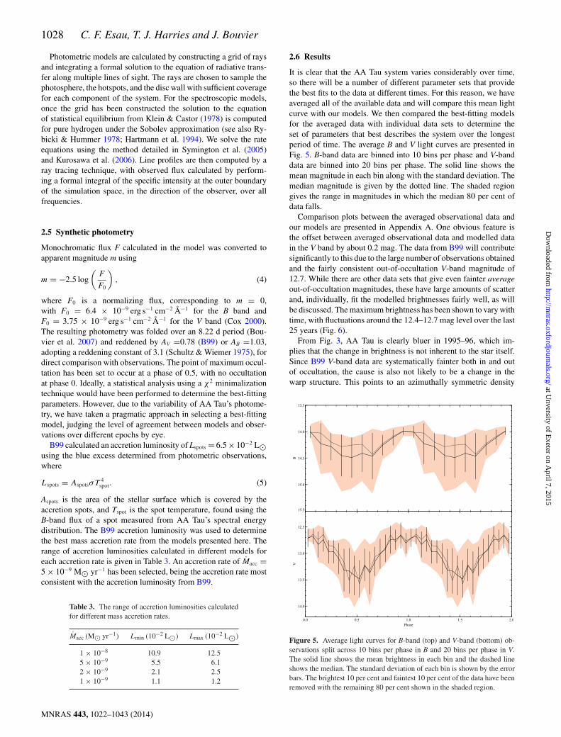
It is clear that the AA Tau system varies considerably over time,so there will be a number of different parameter sets that providethe best fits to the data at different times. For this reason, we haveaveraged all of the available data and will compare this mean lightcurve with our models. We then compared the best-fitting modelsfor the averaged data with individual data sets to determine theset of parameters that best describes the system over the longestperiod of time. The average B and V light curves are presented inFig. 5. B-band data are binned into 10 bins per phase and V-banddata are binned into 20 bins per phase. The solid line shows themean magnitude in each bin along with the standard deviation. Themedian magnitude is given by the dotted line. The shaded regiongives the range in magnitudes in which the median 80 per cent ofdata falls.
Comparison plots between the averaged observational data andour models are presented in Appendix A. One obvious feature isthe offset between averaged observational data and modelled datain the V band by about 0.2 mag. The data from B99 will contributesignificantly to this due to the large number of observations obtainedand the fairly consistent out-of-occultation V-band magnitude of12.7. While there are other data sets that give even fainter averageout-of-occultation magnitudes, these have large amounts of scatterand, individually, fit the modelled brightnesses fairly well, as willbe discussed. The maximum brightness has been shown to vary withtime, with fluctuations around the 12.4–12.7 mag level over the last25 years (Fig. 6).
From Fig. 3, AA Tau is clearly bluer in 1995–96, which im-plies that the change in brightness is not inherent to the star itself.Since B99 V-band data are systematically fainter both in and outof occultation, the cause is also not likely to be a change in thewarp structure. This points to an azimuthally symmetric density
Figure 5. Average light curves for B-band (top) and V-band (bottom) ob-servations split across 10 bins per phase in B and 20 bins per phase in V.The solid line shows the mean brightness in each bin and the dashed lineshows the median. The standard deviation of each bin is shown by the errorbars. The brightest 10 per cent and faintest 10 per cent of the data have beenremoved with the remaining 80 per cent shown in the shaded region.
MNRAS 443, 1022–1043 (2014)
at Unversity of E
xeter on April 7, 2015
http://mnras.oxfordjournals.org/
Dow
nloaded from
Radiative transfer modelling of AA Tau 1029
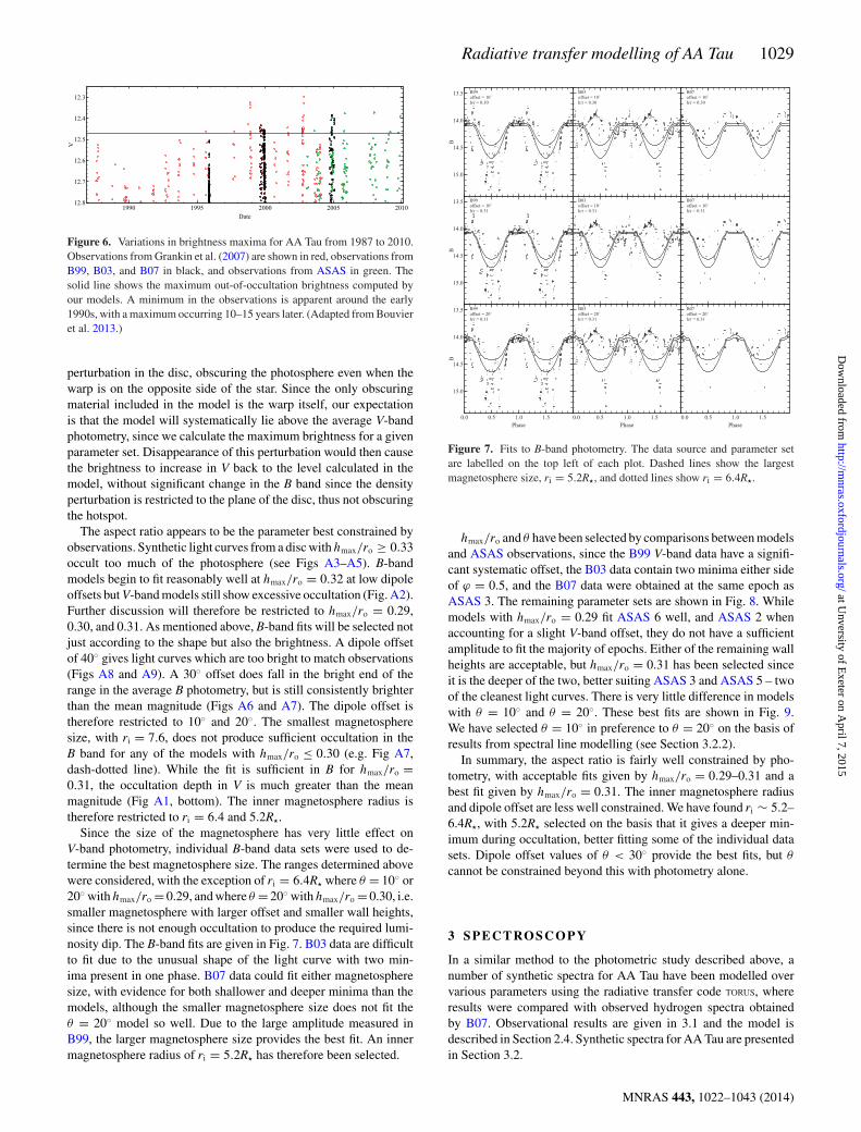
Figure 6. Variations in brightness maxima for AA Tau from 1987 to 2010.Observations from Grankin et al. (2007) are shown in red, observations fromB99, B03, and B07 in black, and observations from ASAS in green. Thesolid line shows the maximum out-of-occultation brightness computed byour models. A minimum in the observations is apparent around the early1990s, with a maximum occurring 10–15 years later. (Adapted from Bouvieret al. 2013.)
perturbation in the disc, obscuring the photosphere even when thewarp is on the opposite side of the star. Since the only obscuringmaterial included in the model is the warp itself, our expectationis that the model will systematically lie above the average V-bandphotometry, since we calculate the maximum brightness for a givenparameter set. Disappearance of this perturbation would then causethe brightness to increase in V back to the level calculated in themodel, without significant change in the B band since the densityperturbation is restricted to the plane of the disc, thus not obscuringthe hotspot.
The aspect ratio appears to be the parameter best constrained byobservations. Synthetic light curves from a disc with hmax/ro ≥ 0.33occult too much of the photosphere (see Figs A3–A5). B-bandmodels begin to fit reasonably well at hmax/ro = 0.32 at low dipoleoffsets but V-band models still show excessive occultation (Fig. A2).Further discussion will therefore be restricted to hmax/ro = 0.29,0.30, and 0.31. As mentioned above, B-band fits will be selected notjust according to the shape but also the brightness. A dipole offsetof 40◦ gives light curves which are too bright to match observations(Figs A8 and A9). A 30◦ offset does fall in the bright end of therange in the average B photometry, but is still consistently brighterthan the mean magnitude (Figs A6 and A7). The dipole offset istherefore restricted to 10◦ and 20◦. The smallest magnetospheresize, with ri = 7.6, does not produce sufficient occultation in theB band for any of the models with hmax/ro ≤ 0.30 (e.g. Fig A7,dash-dotted line). While the fit is sufficient in B for hmax/ro =0.31, the occultation depth in V is much greater than the meanmagnitude (Fig A1, bottom). The inner magnetosphere radius istherefore restricted to ri = 6.4 and 5.2R�.
Since the size of the magnetosphere has very little effect onV-band photometry, individual B-band data sets were used to de-termine the best magnetosphere size. The ranges determined abovewere considered, with the exception of ri = 6.4R� where θ = 10◦ or20◦ with hmax/ro = 0.29, and where θ = 20◦ with hmax/ro = 0.30, i.e.smaller magnetosphere with larger offset and smaller wall heights,since there is not enough occultation to produce the required lumi-nosity dip. The B-band fits are given in Fig. 7. B03 data are difficultto fit due to the unusual shape of the light curve with two min-ima present in one phase. B07 data could fit either magnetospheresize, with evidence for both shallower and deeper minima than themodels, although the smaller magnetosphere size does not fit theθ = 20◦ model so well. Due to the large amplitude measured inB99, the larger magnetosphere size provides the best fit. An innermagnetosphere radius of ri = 5.2R� has therefore been selected.
Figure 7. Fits to B-band photometry. The data source and parameter setare labelled on the top left of each plot. Dashed lines show the largestmagnetosphere size, ri = 5.2R�, and dotted lines show ri = 6.4R�.
hmax/ro and θ have been selected by comparisons between modelsand ASAS observations, since the B99 V-band data have a signifi-cant systematic offset, the B03 data contain two minima either sideof ϕ = 0.5, and the B07 data were obtained at the same epoch asASAS 3. The remaining parameter sets are shown in Fig. 8. Whilemodels with hmax/ro = 0.29 fit ASAS 6 well, and ASAS 2 whenaccounting for a slight V-band offset, they do not have a sufficientamplitude to fit the majority of epochs. Either of the remaining wallheights are acceptable, but hmax/ro = 0.31 has been selected sinceit is the deeper of the two, better suiting ASAS 3 and ASAS 5 – twoof the cleanest light curves. There is very little difference in modelswith θ = 10◦ and θ = 20◦. These best fits are shown in Fig. 9.We have selected θ = 10◦ in preference to θ = 20◦ on the basis ofresults from spectral line modelling (see Section 3.2.2).
In summary, the aspect ratio is fairly well constrained by pho-tometry, with acceptable fits given by hmax/ro = 0.29–0.31 and abest fit given by hmax/ro = 0.31. The inner magnetosphere radiusand dipole offset are less well constrained. We have found ri ∼ 5.2–6.4R�, with 5.2R� selected on the basis that it gives a deeper min-imum during occultation, better fitting some of the individual datasets. Dipole offset values of θ < 30◦ provide the best fits, but θ
cannot be constrained beyond this with photometry alone.
3 SPEC TRO SC O PY
In a similar method to the photometric study described above, anumber of synthetic spectra for AA Tau have been modelled overvarious parameters using the radiative transfer code TORUS, whereresults were compared with observed hydrogen spectra obtainedby B07. Observational results are given in 3.1 and the model isdescribed in Section 2.4. Synthetic spectra for AA Tau are presentedin Section 3.2.
MNRAS 443, 1022–1043 (2014)
at Unversity of E
xeter on April 7, 2015
http://mnras.oxfordjournals.org/
Dow
nloaded from
1030 C. F. Esau, T. J. Harries and J. Bouvier
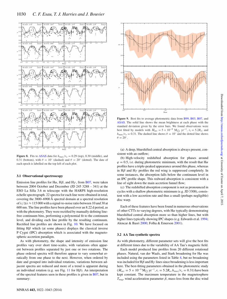
Figure 8. Fits to ASAS data for hmax/ro = 0.29 (top), 0.30 (middle), and0.31 (bottom), with θ = 10◦ (dashed) and θ = 20◦ (dotted). The date ofeach epoch is labelled on the top left of each plot.
3.1 Observational spectroscopy
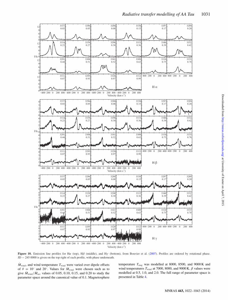
Emission line profiles for Hα, Hβ, and Hγ , from B07, were takenbetween 2004 October and December (JD 245 3288 – 341) at theESO La Silla 3.6 m telescope with the HARPS high-resolutionechelle spectrograph. 22 spectra for each line were obtained in total,covering the 3800–6900 Å spectral domain at a spectral resolutionof λ/�λ ≈ 115 000 with a signal-to-noise ratio between 10 and 30 at600 nm. The line profiles have been phased over an 8.22 d period, aswith the photometry. They were rectified by manually defining line-free continuum bins, performing a polynomial fit to the continuumlevel, and dividing each line profile by the resulting continuum.Rectified line profiles are shown in Fig. 10. We have focused onfitting Hβ which (at some phases) displays the classical inverseP Cygni (IPC) absorption which is associated with the magneto-spheric accretion paradigm.
As with photometry, the shape and intensity of emission lineprofiles vary over short time-scales, with variations often appar-ent between profiles separated by just one or two rotations. Thephase ordered spectra will therefore appear to vary somewhat er-ratically from one phase to the next. However, when ordered bydate and grouped into individual rotations, variations between ad-jacent spectra are reduced and more of a trend is apparent duringan individual rotation (e.g. see Fig. 11 for Hβ). An interpretationof the spectral features seen in these profiles is given in B07, but insummary:
Figure 9. Best fits to average photometric data from B99, B03, B07, andASAS. The solid line shows the mean brightness at each phase with thestandard deviation given by the error bars. We found observations werebest fitted by models with Macc = 5 × 10⁻⁹ M� yr−1, ri = 5.2R�, andhmax/ro = 0.31. The dashed line shows θ = 10◦ and the dotted line showsθ = 20◦.
(a) A deep, blueshifted central absorption is always present, con-sistent with an outflow;
(b) High-velocity redshifted absorption for phases aroundϕ = 0.5, i.e. during photometric minimum, with the result that Hα
profiles have a triple-peaked appearance around this phase, whereasin Hβ and Hγ profiles the red wing is suppressed completely. Insome instances, the absorption falls below the continuum level inan IPC profile shape. This redward absorption is consistent with aline of sight down the main accretion funnel flow;
(c) The redshifted absorption component is not as pronounced incycles with a shallow photometric minimum (e.g. JD 3308), consis-tent with a low accretion rate and thus a small (perhaps negligible)disc warp.
Each of these features have been found in numerous observationsof other CTTs to varying degrees, with Hα typically demonstratingblueshifted central absorption more so than higher lines, but withhigher lines typically showing IPC shapes (e.g. Edwards et al. 1994;Alencar & Basri 2000; Folha & Emerson 2001).
3.2 AA Tau synthetic spectra
As with photometry, different parameter sets will give the best fitsat different times due to the variability of AA Tau’s magnetic field.
Each model produced line profiles from 20 different rotationalphases. Natural, van der Waals, and Stark broadening for Hα wasincluded using the parameters listed in Table 4, but no broadeningwas included for Hβ and Hγ lines since broadening is less importanthere. The best-fitting parameters obtained in the photometric study(Macc = 5 × 10⁻⁹ M� yr−1, ri = 5.2R�, hmax/ro = 0.31) have beenkept constant. The maximum temperature in the magnetosphereTmag, wind acceleration parameter β, mass-loss from the disc wind
MNRAS 443, 1022–1043 (2014)
at Unversity of E
xeter on April 7, 2015
http://mnras.oxfordjournals.org/
Dow
nloaded from
Radiative transfer modelling of AA Tau 1031
Figure 10. Emission line profiles for Hα (top), Hβ (middle), and Hγ (bottom), from Bouvier et al. (2007). Profiles are ordered by rotational phase.JD − 245 0000 is given on the top right of each profile, with phase underneath.
Mwind, and wind temperature Twind were varied over dipole offsetsof θ = 10◦ and 20◦. Values for Mwind were chosen such as togive Mwind/Macc values of 0.05, 0.10, 0.15, and 0.20 to study theparameter space around the canonical value of 0.1. Magnetosphere
temperature Tmag was modelled at 8000, 8500, and 9000 K andwind temperatures Twind at 7000, 8000, and 9000 K. β values weremodelled at 0.5, 1.0, and 2.0. The full range of parameter space ispresented in Table 4.
MNRAS 443, 1022–1043 (2014)
at Unversity of E
xeter on April 7, 2015
http://mnras.oxfordjournals.org/
Dow
nloaded from
1032 C. F. Esau, T. J. Harries and J. Bouvier
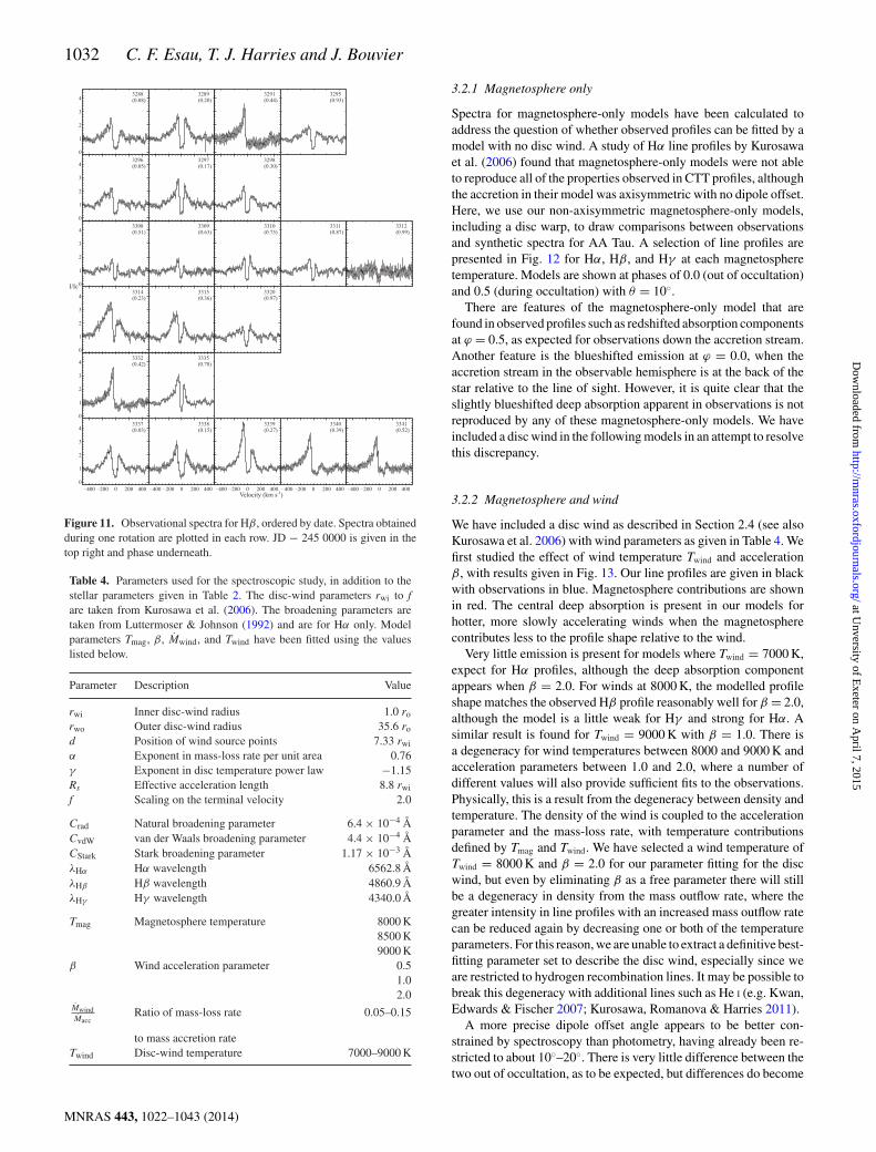
Figure 11. Observational spectra for Hβ, ordered by date. Spectra obtainedduring one rotation are plotted in each row. JD − 245 0000 is given in thetop right and phase underneath.
Table 4. Parameters used for the spectroscopic study, in addition to thestellar parameters given in Table 2. The disc-wind parameters rwi to fare taken from Kurosawa et al. (2006). The broadening parameters aretaken from Luttermoser & Johnson (1992) and are for Hα only. Modelparameters Tmag, β, Mwind, and Twind have been fitted using the valueslisted below.
Parameter Description Value
rwi Inner disc-wind radius 1.0 ro
rwo Outer disc-wind radius 35.6 ro
d Position of wind source points 7.33 rwi
α Exponent in mass-loss rate per unit area 0.76γ Exponent in disc temperature power law −1.15Rs Effective acceleration length 8.8 rwi
f Scaling on the terminal velocity 2.0
Crad Natural broadening parameter 6.4 × 10⁻⁴ ÅCvdW van der Waals broadening parameter 4.4 × 10⁻⁴ ÅCStark Stark broadening parameter 1.17 × 10⁻³ ÅλHα Hα wavelength 6562.8 ÅλHβ Hβ wavelength 4860.9 ÅλHγ Hγ wavelength 4340.0 Å
Tmag Magnetosphere temperature 8000 K8500 K9000 K
β Wind acceleration parameter 0.51.02.0
MwindMacc
Ratio of mass-loss rate 0.05–0.15
to mass accretion rateTwind Disc-wind temperature 7000–9000 K
3.2.1 Magnetosphere only
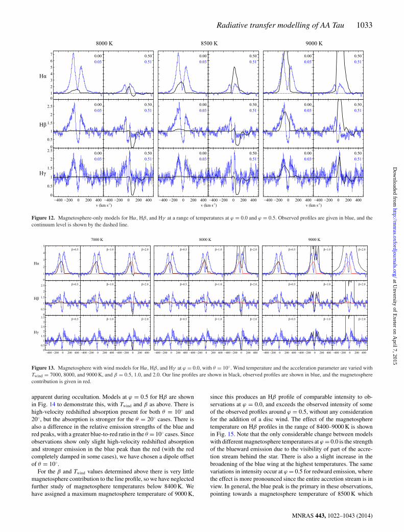
Spectra for magnetosphere-only models have been calculated toaddress the question of whether observed profiles can be fitted by amodel with no disc wind. A study of Hα line profiles by Kurosawaet al. (2006) found that magnetosphere-only models were not ableto reproduce all of the properties observed in CTT profiles, althoughthe accretion in their model was axisymmetric with no dipole offset.Here, we use our non-axisymmetric magnetosphere-only models,including a disc warp, to draw comparisons between observationsand synthetic spectra for AA Tau. A selection of line profiles arepresented in Fig. 12 for Hα, Hβ, and Hγ at each magnetospheretemperature. Models are shown at phases of 0.0 (out of occultation)and 0.5 (during occultation) with θ = 10◦.
There are features of the magnetosphere-only model that arefound in observed profiles such as redshifted absorption componentsat ϕ = 0.5, as expected for observations down the accretion stream.Another feature is the blueshifted emission at ϕ = 0.0, when theaccretion stream in the observable hemisphere is at the back of thestar relative to the line of sight. However, it is quite clear that theslightly blueshifted deep absorption apparent in observations is notreproduced by any of these magnetosphere-only models. We haveincluded a disc wind in the following models in an attempt to resolvethis discrepancy.
3.2.2 Magnetosphere and wind
We have included a disc wind as described in Section 2.4 (see alsoKurosawa et al. 2006) with wind parameters as given in Table 4. Wefirst studied the effect of wind temperature Twind and accelerationβ, with results given in Fig. 13. Our line profiles are given in blackwith observations in blue. Magnetosphere contributions are shownin red. The central deep absorption is present in our models forhotter, more slowly accelerating winds when the magnetospherecontributes less to the profile shape relative to the wind.
Very little emission is present for models where Twind = 7000 K,expect for Hα profiles, although the deep absorption componentappears when β = 2.0. For winds at 8000 K, the modelled profileshape matches the observed Hβ profile reasonably well for β = 2.0,although the model is a little weak for Hγ and strong for Hα. Asimilar result is found for Twind = 9000 K with β = 1.0. There isa degeneracy for wind temperatures between 8000 and 9000 K andacceleration parameters between 1.0 and 2.0, where a number ofdifferent values will also provide sufficient fits to the observations.Physically, this is a result from the degeneracy between density andtemperature. The density of the wind is coupled to the accelerationparameter and the mass-loss rate, with temperature contributionsdefined by Tmag and Twind. We have selected a wind temperature ofTwind = 8000 K and β = 2.0 for our parameter fitting for the discwind, but even by eliminating β as a free parameter there will stillbe a degeneracy in density from the mass outflow rate, where thegreater intensity in line profiles with an increased mass outflow ratecan be reduced again by decreasing one or both of the temperatureparameters. For this reason, we are unable to extract a definitive best-fitting parameter set to describe the disc wind, especially since weare restricted to hydrogen recombination lines. It may be possible tobreak this degeneracy with additional lines such as He I (e.g. Kwan,Edwards & Fischer 2007; Kurosawa, Romanova & Harries 2011).
A more precise dipole offset angle appears to be better con-strained by spectroscopy than photometry, having already been re-stricted to about 10◦–20◦. There is very little difference between thetwo out of occultation, as to be expected, but differences do become
MNRAS 443, 1022–1043 (2014)
at Unversity of E
xeter on April 7, 2015
http://mnras.oxfordjournals.org/
Dow
nloaded from
Radiative transfer modelling of AA Tau 1033
Figure 12. Magnetosphere-only models for Hα, Hβ, and Hγ at a range of temperatures at ϕ = 0.0 and ϕ = 0.5. Observed profiles are given in blue, and thecontinuum level is shown by the dashed line.
Figure 13. Magnetosphere with wind models for Hα, Hβ, and Hγ at ϕ = 0.0, with θ = 10◦. Wind temperature and the acceleration parameter are varied withTwind = 7000, 8000, and 9000 K, and β = 0.5, 1.0, and 2.0. Our line profiles are shown in black, observed profiles are shown in blue, and the magnetospherecontribution is given in red.
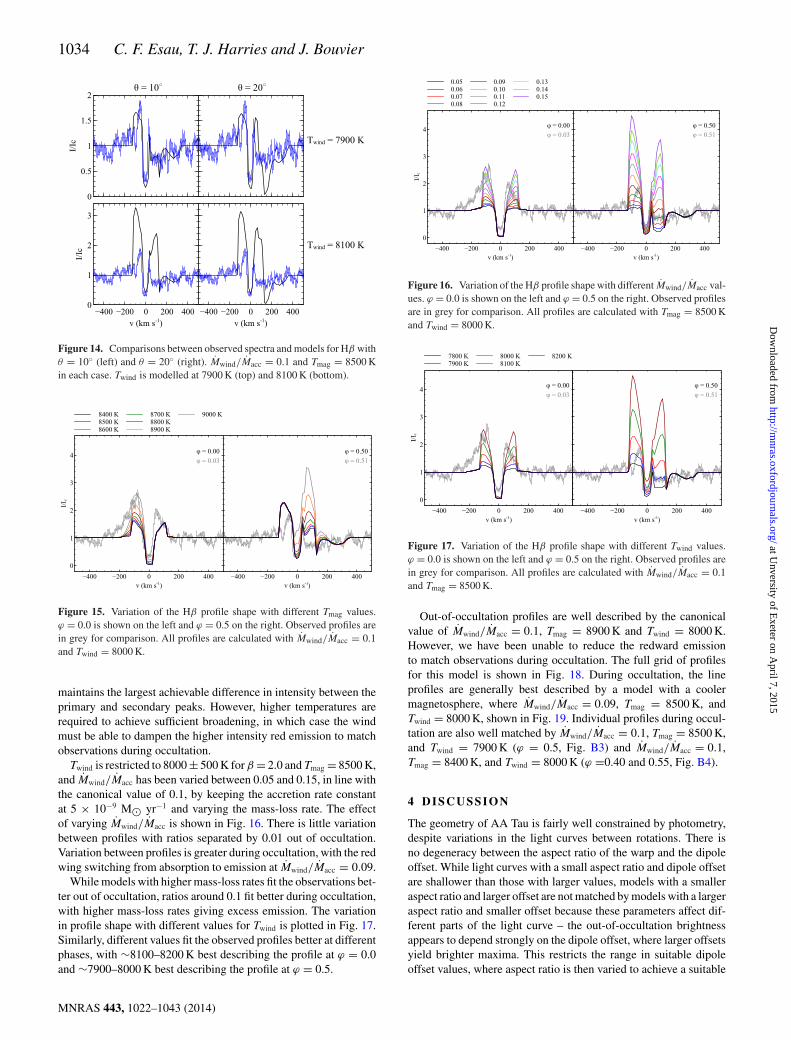
apparent during occultation. Models at ϕ = 0.5 for Hβ are shownin Fig. 14 to demonstrate this, with Twind and β as above. There ishigh-velocity redshifted absorption present for both θ = 10◦ and20◦, but the absorption is stronger for the θ = 20◦ cases. There isalso a difference in the relative emission strengths of the blue andred peaks, with a greater blue-to-red ratio in the θ = 10◦ cases. Sinceobservations show only slight high-velocity redshifted absorptionand stronger emission in the blue peak than the red (with the redcompletely damped in some cases), we have chosen a dipole offsetof θ = 10◦.
For the β and Twind values determined above there is very littlemagnetosphere contribution to the line profile, so we have neglectedfurther study of magnetosphere temperatures below 8400 K. Wehave assigned a maximum magnetosphere temperature of 9000 K,
since this produces an Hβ profile of comparable intensity to ob-servations at ϕ = 0.0, and exceeds the observed intensity of someof the observed profiles around ϕ = 0.5, without any considerationfor the addition of a disc wind. The effect of the magnetospheretemperature on Hβ profiles in the range of 8400–9000 K is shownin Fig. 15. Note that the only considerable change between modelswith different magnetosphere temperatures at ϕ = 0.0 is the strengthof the blueward emission due to the visibility of part of the accre-tion stream behind the star. There is also a slight increase in thebroadening of the blue wing at the highest temperatures. The samevariations in intensity occur at ϕ = 0.5 for redward emission, wherethe effect is more pronounced since the entire accretion stream is inview. In general, the blue peak is the primary in these observations,pointing towards a magnetosphere temperature of 8500 K which
MNRAS 443, 1022–1043 (2014)
at Unversity of E
xeter on April 7, 2015
http://mnras.oxfordjournals.org/
Dow
nloaded from
1034 C. F. Esau, T. J. Harries and J. Bouvier
Figure 14. Comparisons between observed spectra and models for Hβ withθ = 10◦ (left) and θ = 20◦ (right). Mwind/Macc = 0.1 and Tmag = 8500 Kin each case. Twind is modelled at 7900 K (top) and 8100 K (bottom).
Figure 15. Variation of the Hβ profile shape with different Tmag values.ϕ = 0.0 is shown on the left and ϕ = 0.5 on the right. Observed profiles arein grey for comparison. All profiles are calculated with Mwind/Macc = 0.1and Twind = 8000 K.
maintains the largest achievable difference in intensity between theprimary and secondary peaks. However, higher temperatures arerequired to achieve sufficient broadening, in which case the windmust be able to dampen the higher intensity red emission to matchobservations during occultation.
Twind is restricted to 8000 ± 500 K for β = 2.0 and Tmag = 8500 K,and Mwind/Macc has been varied between 0.05 and 0.15, in line withthe canonical value of 0.1, by keeping the accretion rate constantat 5 × 10⁻⁹ M� yr−1 and varying the mass-loss rate. The effectof varying Mwind/Macc is shown in Fig. 16. There is little variationbetween profiles with ratios separated by 0.01 out of occultation.Variation between profiles is greater during occultation, with the redwing switching from absorption to emission at Mwind/Macc = 0.09.
While models with higher mass-loss rates fit the observations bet-ter out of occultation, ratios around 0.1 fit better during occultation,with higher mass-loss rates giving excess emission. The variationin profile shape with different values for Twind is plotted in Fig. 17.Similarly, different values fit the observed profiles better at differentphases, with ∼8100–8200 K best describing the profile at ϕ = 0.0and ∼7900–8000 K best describing the profile at ϕ = 0.5.
Figure 16. Variation of the Hβ profile shape with different Mwind/Macc val-ues. ϕ = 0.0 is shown on the left and ϕ = 0.5 on the right. Observed profilesare in grey for comparison. All profiles are calculated with Tmag = 8500 Kand Twind = 8000 K.
Figure 17. Variation of the Hβ profile shape with different Twind values.ϕ = 0.0 is shown on the left and ϕ = 0.5 on the right. Observed profiles arein grey for comparison. All profiles are calculated with Mwind/Macc = 0.1and Tmag = 8500 K.
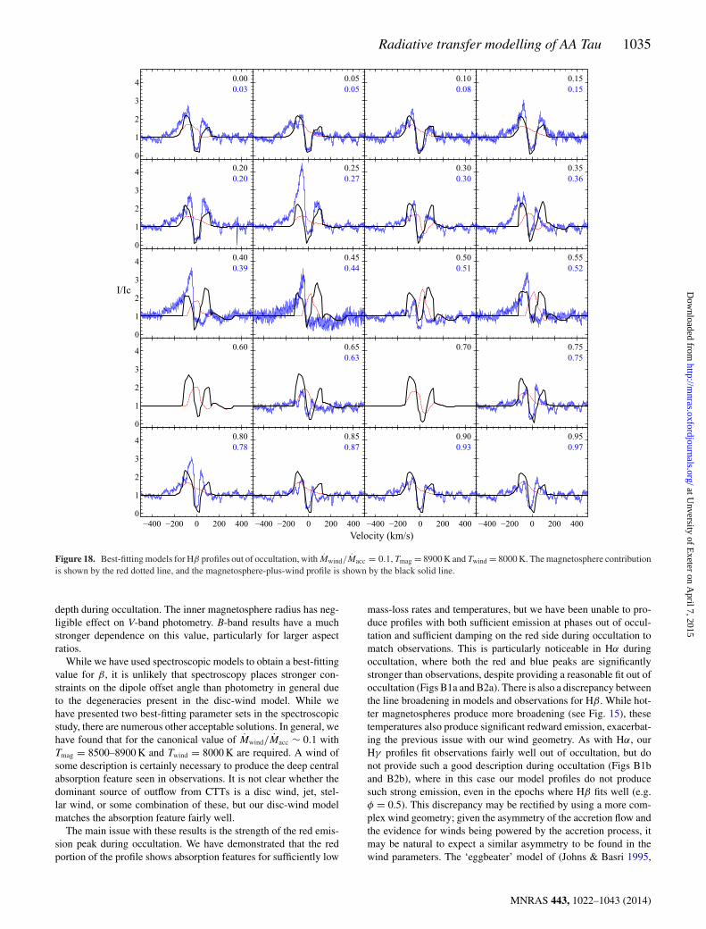
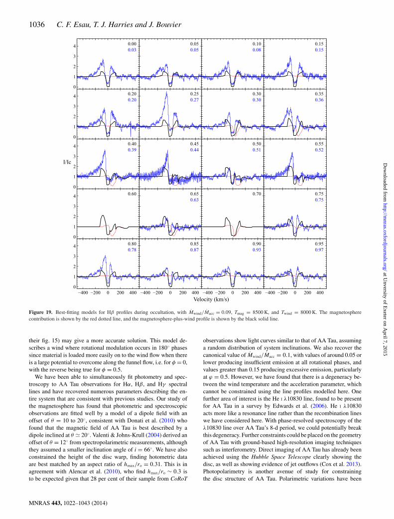
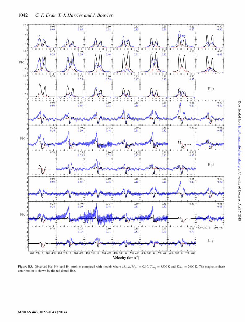
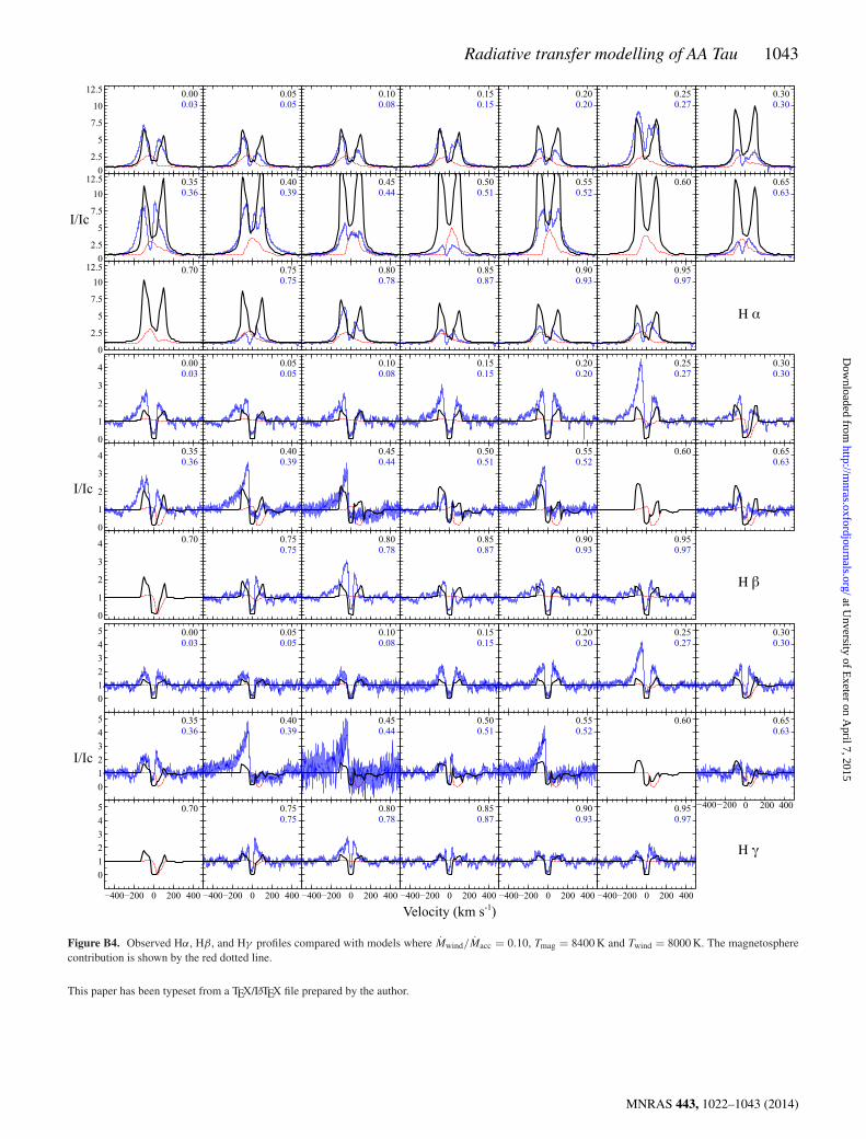
Out-of-occultation profiles are well described by the canonicalvalue of Mwind/Macc = 0.1, Tmag = 8900 K and Twind = 8000 K.However, we have been unable to reduce the redward emissionto match observations during occultation. The full grid of profilesfor this model is shown in Fig. 18. During occultation, the lineprofiles are generally best described by a model with a coolermagnetosphere, where Mwind/Macc = 0.09, Tmag = 8500 K, andTwind = 8000 K, shown in Fig. 19. Individual profiles during occul-tation are also well matched by Mwind/Macc = 0.1, Tmag = 8500 K,and Twind = 7900 K (ϕ = 0.5, Fig. B3) and Mwind/Macc = 0.1,Tmag = 8400 K, and Twind = 8000 K (ϕ =0.40 and 0.55, Fig. B4).
4 D I SCUSSI ON
The geometry of AA Tau is fairly well constrained by photometry,despite variations in the light curves between rotations. There isno degeneracy between the aspect ratio of the warp and the dipoleoffset. While light curves with a small aspect ratio and dipole offsetare shallower than those with larger values, models with a smalleraspect ratio and larger offset are not matched by models with a largeraspect ratio and smaller offset because these parameters affect dif-ferent parts of the light curve – the out-of-occultation brightnessappears to depend strongly on the dipole offset, where larger offsetsyield brighter maxima. This restricts the range in suitable dipoleoffset values, where aspect ratio is then varied to achieve a suitable
MNRAS 443, 1022–1043 (2014)
at Unversity of E
xeter on April 7, 2015
http://mnras.oxfordjournals.org/
Dow
nloaded from
Radiative transfer modelling of AA Tau 1035
Figure 18. Best-fitting models for Hβ profiles out of occultation, with Mwind/Macc = 0.1, Tmag = 8900 K and Twind = 8000 K. The magnetosphere contributionis shown by the red dotted line, and the magnetosphere-plus-wind profile is shown by the black solid line.
depth during occultation. The inner magnetosphere radius has neg-ligible effect on V-band photometry. B-band results have a muchstronger dependence on this value, particularly for larger aspectratios.
While we have used spectroscopic models to obtain a best-fittingvalue for β, it is unlikely that spectroscopy places stronger con-straints on the dipole offset angle than photometry in general dueto the degeneracies present in the disc-wind model. While wehave presented two best-fitting parameter sets in the spectroscopicstudy, there are numerous other acceptable solutions. In general, wehave found that for the canonical value of Mwind/Macc ∼ 0.1 withTmag = 8500–8900 K and Twind = 8000 K are required. A wind ofsome description is certainly necessary to produce the deep centralabsorption feature seen in observations. It is not clear whether thedominant source of outflow from CTTs is a disc wind, jet, stel-lar wind, or some combination of these, but our disc-wind modelmatches the absorption feature fairly well.
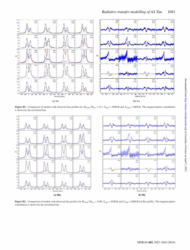
The main issue with these results is the strength of the red emis-sion peak during occultation. We have demonstrated that the redportion of the profile shows absorption features for sufficiently low
mass-loss rates and temperatures, but we have been unable to pro-duce profiles with both sufficient emission at phases out of occul-tation and sufficient damping on the red side during occultation tomatch observations. This is particularly noticeable in Hα duringoccultation, where both the red and blue peaks are significantlystronger than observations, despite providing a reasonable fit out ofoccultation (Figs B1a and B2a). There is also a discrepancy betweenthe line broadening in models and observations for Hβ. While hot-ter magnetospheres produce more broadening (see Fig. 15), thesetemperatures also produce significant redward emission, exacerbat-ing the previous issue with our wind geometry. As with Hα, ourHγ profiles fit observations fairly well out of occultation, but donot provide such a good description during occultation (Figs B1band B2b), where in this case our model profiles do not producesuch strong emission, even in the epochs where Hβ fits well (e.g.φ = 0.5). This discrepancy may be rectified by using a more com-plex wind geometry; given the asymmetry of the accretion flow andthe evidence for winds being powered by the accretion process, itmay be natural to expect a similar asymmetry to be found in thewind parameters. The ‘eggbeater’ model of (Johns & Basri 1995,
MNRAS 443, 1022–1043 (2014)
at Unversity of E
xeter on April 7, 2015
http://mnras.oxfordjournals.org/
Dow
nloaded from
1036 C. F. Esau, T. J. Harries and J. Bouvier
Figure 19. Best-fitting models for Hβ profiles during occultation, with Mwind/Macc = 0.09, Tmag = 8500 K, and Twind = 8000 K. The magnetospherecontribution is shown by the red dotted line, and the magnetosphere-plus-wind profile is shown by the black solid line.
their fig. 15) may give a more accurate solution. This model de-scribes a wind where rotational modulation occurs in 180◦ phasessince material is loaded more easily on to the wind flow when thereis a large potential to overcome along the funnel flow, i.e. for φ = 0,with the reverse being true for φ = 0.5.
We have been able to simultaneously fit photometry and spec-troscopy to AA Tau observations for Hα, Hβ, and Hγ spectrallines and have recovered numerous parameters describing the en-tire system that are consistent with previous studies. Our study ofthe magnetosphere has found that photometric and spectroscopicobservations are fitted well by a model of a dipole field with anoffset of θ = 10 to 20◦, consistent with Donati et al. (2010) whofound that the magnetic field of AA Tau is best described by adipole inclined at θ � 20◦. Valenti & Johns-Krull (2004) derived anoffset of θ = 12◦ from spectropolarimetric measurements, althoughthey assumed a smaller inclination angle of i = 66◦. We have alsoconstrained the height of the disc warp, finding hotometric dataare best matched by an aspect ratio of hmax/ro = 0.31. This is inagreement with Alencar et al. (2010), who find hmax/ro ∼ 0.3 isto be expected given that 28 per cent of their sample from CoRoT
observations show light curves similar to that of AA Tau, assuminga random distribution of system inclinations. We also recover thecanonical value of Mwind/Macc = 0.1, with values of around 0.05 orlower producing insufficient emission at all rotational phases, andvalues greater than 0.15 producing excessive emission, particularlyat ϕ = 0.5. However, we have found that there is a degeneracy be-tween the wind temperature and the acceleration parameter, whichcannot be constrained using the line profiles modelled here. Onefurther area of interest is the He I λ10830 line, found to be presentfor AA Tau in a survey by Edwards et al. (2006). He I λ10830acts more like a resonance line rather than the recombination lineswe have considered here. With phase-resolved spectroscopy of theλ10830 line over AA Tau’s 8-d period, we could potentially breakthis degeneracy. Further constraints could be placed on the geometryof AA Tau with ground-based high-resolution imaging techniquessuch as interferometry. Direct imaging of AA Tau has already beenachieved using the Hubble Space Telescope clearly showing thedisc, as well as showing evidence of jet outflows (Cox et al. 2013).Photopolarimetry is another avenue of study for constrainingthe disc structure of AA Tau. Polarimetric variations have been
MNRAS 443, 1022–1043 (2014)
at Unversity of E
xeter on April 7, 2015
http://mnras.oxfordjournals.org/
Dow
nloaded from
Radiative transfer modelling of AA Tau 1037
observed by B99, B03 and Menard et al. (2003), who found thatpolarization is strongest when the system is faint, consistent withthe presence of additional disc material enhancing the amount ofpolarization. Photopolarimetry of the warp modelled by O’Sullivanet al. (2005) yields a warp position slightly interior to the coro-tation radius, with their warped disc model reproducing observedbrightness and polarization variations well.
5 SU M M A RY
While initially variations in the light curves of CTTs were thoughtto be rare, such features have been shown to be present in at least28 per cent of light curves (Alencar et al. 2010). AA Tau was thefirst CTT observed to exhibit such photometric variations, and hasbeen included in, and the subject of, many observational campaignssince (Gullbring et al. 1998; B99; B07; Bouvier et al. 2013; Grankinet al. 2007; Johns-Krull 2007; Donati et al. 2010). Using the radia-tive transfer code TORUS, we have produced synthetic photometryand spectroscopy which were compared to photometric and spectro-scopic observations from B99, B03, and B07, as well as photome-try from ASAS, to constrain geometric and physical parameters forAA Tau, simultaneously fitting photometry and spectroscopy. Thegeometry of the system varies over time as the magnetic field linesemanating from the star break and reconnect, so while our best-fitting parameter sets have been found to best describe the systemon average, different values will give superior fits at different times.Photometric models were used to constrain the mass accretion rate,the maximum height of the inner disc warp, the dipole offset, andthe inner radius of the magnetosphere. Spectroscopic models wereused to further constrain the dipole offset, and to investigate themass-loss rate from a disc wind, the temperature of the wind, andthe temperature of the magnetosphere. We found that models witha mass accretion rate of ∼5 × 10⁻⁹ M� yr−1 yielded an accretionluminosity of up to 6.1 × 10⁻² L�, consistent with the value of6.5 × 10−2 L� calculated by B99. This accretion rate is consistentwith the range of 2–7 × 10⁻⁹ M� yr−1 calculated from Hα andHβ line fluxes in Bouvier et al. (2013). We collated all publiclyavailable B- and V-band photometry and found average light curvesare best described by hmax/ro ∼ 0.31 and θ = 10◦–20◦, consis-tent with B99, who also derived hmax/ro = 0.3 (see also Terquem& Papaloizou 2000), and Alencar et al. (2010), who also foundhmax/ro ∼ 0.3 for AA Tau-like light curves. The range in dipoleoffsets is consistent with Donati et al. (2010), who found θ = 20◦,although our spectroscopic models favour θ = 10◦. A disc wind isrequired to recover the line shapes observed. Although degeneraciesbetween density and temperature in the disc wind prevent the deter-mination of absolute values, we have found that the canonical valuefor mass-loss rate to mass accretion rate of 0.1 is recovered. Discwind and magnetosphere temperatures of Twind ∼ 7900–8000 K andTmag ∼ 8400–8500 K have been established.
A future study of the He I λ10830 line for AA Tau would bebeneficial to further constrain the outflow mechanism. Developinga more complex, azimuthally asymmetric disc-wind calculation inTORUS may also account for the variations between the best-fittingwind parameters at different phases encountered here. However,we cannot progress much further than this by fitting spectra alone.Extra leverage may soon be achievable with spectrally resolvedinterferometry, which has already been used successfully to in-fer information about Herbig Ae/Be stars (e.g. Kraus, Preibisch &Ohnaka 2007; Kraus et al. 2008). Current instrumentation is unable
to achieve the sensitivity in both signal to noise and resolution toprobe the small inner region of T Tauri stars, but it remains an excit-ing prospect for the next generation of interferometers. The adventof high-resolution interferometry will allow us to infer spatial in-formation about CTT systems, providing much stronger constraintson a system’s geometry.
AC K N OW L E D G E M E N T S
The calculations for this paper were performed using the Uni-versity of Exeter Supercomputer. We thank the referee for theircomments. CFE acknowledges funding from a College studentshipawarded by The of Exeter, and TJH acknowledges funding fromthe STFC grant ST/J001627/1. Finally, we acknowledge the ASASproject for additional AA Tau photometric data (available online athttp://www.astrouw.edu.pl/asas/).
R E F E R E N C E S
Alencar S. H. P., Basri G., 2000, AJ, 119, 1881Alencar S. H. P. et al., 2010, A&A, 519, A88Appenzeller I., Bertout C., Stahl O., 2005, A&A, 434, 1005Artemenko S. A., Grankin K. N., Petrov P. P., 2012, Astron. Lett., 38, 783Basri G., Bertout C., 1989, ApJ, 341, 340Bertout C., Basri G., Bouvier J., 1988, ApJ, 330, 350Blandford R. D., Payne D. G., 1982, MNRAS, 199, 883Bouvier J. et al., 1999, A&A, 349, 619 (B99)Bouvier J. et al., 2003, A&A, 409, 169 (B03)Bouvier J. et al., 2007, A&A, 463, 1017 (B07)Bouvier J., Grankin K., Ellerbroeck L. E., Bouy H., Barrado D., 2013, A&A,
557, A77Burrows C. J. et al., 1996, ApJ, 473, 437Cabrit S., 2007, in Bouvier J., Appenzeller I., eds, Proc. IAU Symp. 243,
Star-Disk Interaction in Young Stars. Cambridge Univ. Press, Cam-bridge, p. 203
Cabrit S., Edwards S., Strom S. E., Strom K. M., 1990, ApJ, 354, 687Camenzind M., 1990, Rev. Mod. Astron., 3, 234Castor J. I., Lamers H. J. G. L. M., 1979, ApJS, 39, 481Castor J. I., Abbott D. C., Klein R. I., 1975, ApJ, 195, 157Cox A. N., 2000, AllenOs Astrophysical Quantities. Springer, New YorkCox A. W., Grady C. A., Hammel H. B., Hornbeck J., Russell R. W., Stiko
M. L., Woodgate B. E., 2013, ApJ, 762, 40Donati J. F. et al., 2010, MNRAS, 409, 1347Edwards S., Cabrit S., Strom S. E., Heyer I., Strom K. M., Anderson E.,
1987, ApJ, 321, 473Edwards S., Hartigan P., Ghandour L., Andrulis C., 1994, AJ, 108,
1056Edwards S., Fischer W., Hillenbrand L., Kwan J., 2006, ApJ, 646,
319Ferreira J., Dougados C., Cabrit S., 2006, A&A, 453, 785Folha D. F. M., Emerson J. P., 2001, A&A, 365, 90Grankin K. N., Melnikov S. Y., Bouvier J., Herbst W., Shevchenko V. S.,
2007, A&A, 461, 183Gullbring E., Hartmann L., Briceno C., Calvet N., 1998, ApJ, 492,
323Harries T. J., 2000, MNRAS, 315, 722Hartmann L., Hewett R., Calvet N., 1994, ApJ, 426, 669Howarth I. D., 2011, MNRAS, 413, 1515Johns C. M., Basri G., 1995, ApJ, 449, 341Johns-Krull C. M., 2007, ApJ, 664, 975Kenyon S. J., Hartmann L., 1995, ApJS, 101, 117Klein R. I., Castor J. I., 1978, ApJ, 220, 902
MNRAS 443, 1022–1043 (2014)
at Unversity of E
xeter on April 7, 2015
http://mnras.oxfordjournals.org/
Dow
nloaded from
1038 C. F. Esau, T. J. Harries and J. Bouvier
Knigge C., Woods J. A., Drew J. E., 1995, MNRAS, 273, 225Konigl A., 1991, ApJ, 370, L39Konigl A., Pudritz R. E., 2000, in Mannings V., Boss A. P., Russell
S. S., eds, Protostars and Planets IV. Univ. Arizona Press, Tucson,p. 759
Kopal Z., 1950, Harv. Coll. Obs. Circ., 454, 1Kraus S., Preibisch T., Ohnaka K., 2007, in Bouvier J., Appenzeller I., eds,
Proc. IAU Symp. 243, Star-Disk Interaction in Young Stars. CambridgeUniv. Press, Cambridge, p. 337
Kraus S. et al., 2008, A&A, 489, 1157Kurosawa R., Harries T. J., Symington N. H., 2006, MNRAS, 370,
580Kurosawa R., Romanova M. M., Harries T. J., 2011, MNRAS, 416,
2623Kwan J., 1997, ApJ, 489, 284Kwan J., Edwards S., Fischer W., 2007, ApJ, 657, 897Long K. S., Knigge C., 2002, ApJ, 579, 725Luttermoser D. G., Johnson H. R., 1992, ApJ, 388, 579Mahdavi A., Kenyon S. J., 1998, ApJ, 497, 342Matt S., Pudritz R. E., 2005, ApJ, 632, L135Menard F., Bouvier J., Dougados C., Mel’nikov S. Y., Grankin K. N., 2003,
A&A, 409, 163Mundt R., 1984, ApJ, 280, 749Muzerolle J., Calvet N., Hartmann L., 1998, ApJ, 492, 743Muzerolle J., Calvet N., Hartmann L., 2001, ApJ, 550, 944O’Sullivan M., Truss M., Walker C., Wood K., Matthews O., Whitney B.,
Bjorkman J. E., 2005, MNRAS, 358, 632Pojmanski G., Pilecki B., Szczygiel D., 2005, Acta Astron., 55, 275
(ASAS)Pudritz R. E., Norman C. A., 1983, ApJ, 274, 677Reipurth B., Pedrosa A., Lago M. T. V. T., 1996, A&AS, 120, 229Rybicki G. B., Hummer D. G., 1978, ApJ, 219, 654Schultz G. V., Wiemer W., 1975, A&A, 43, 133Symington N. H., Harries T. J., Kurosawa R., 2005, MNRAS, 356,
1489Terquem C., Papaloizou J. C. B., 2000, A&A, 360, 1031Valenti J. A., Johns-Krull C. M., 2004, Ap&SS, 292, 619Vrba F. J., Rydgren A. E., Chugainov P. F., Shakovskaya N., Weaver W. B.,
1989, AJ, 97, 483
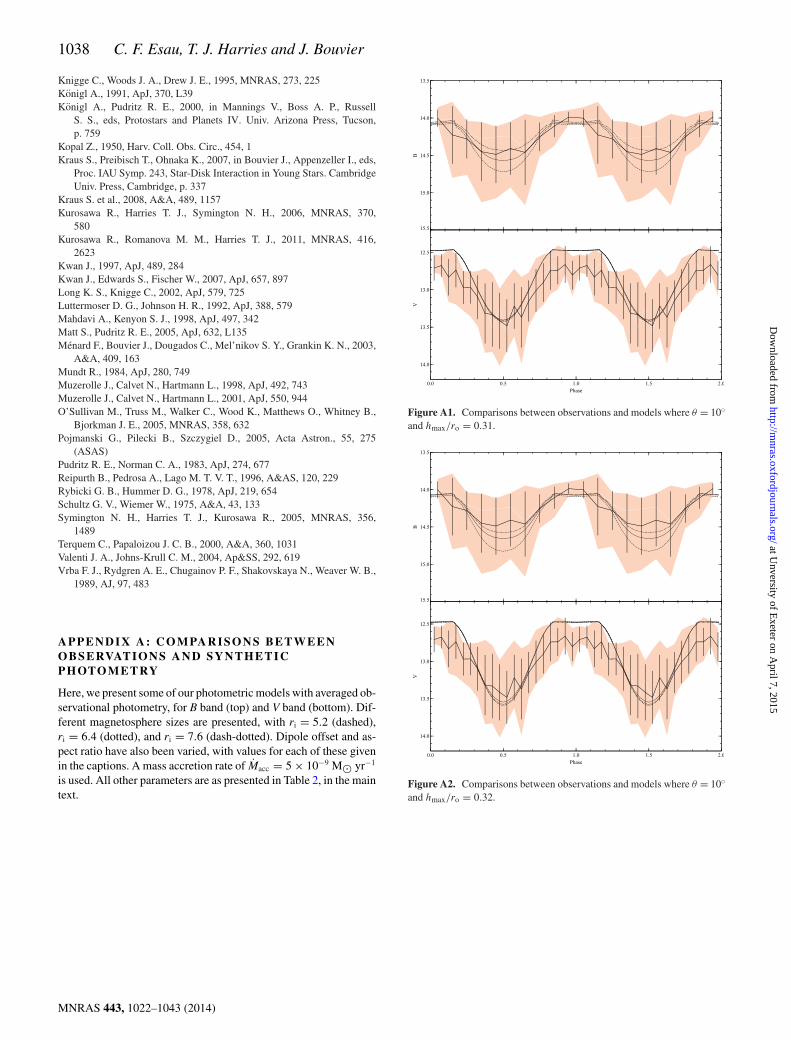
A P P E N D I X A : C O M PA R I S O N S B E T W E E NO B S E RVAT I O N S A N D S Y N T H E T I CP H OTO M E T RY
Here, we present some of our photometric models with averaged ob-servational photometry, for B band (top) and V band (bottom). Dif-ferent magnetosphere sizes are presented, with ri = 5.2 (dashed),ri = 6.4 (dotted), and ri = 7.6 (dash-dotted). Dipole offset and as-pect ratio have also been varied, with values for each of these givenin the captions. A mass accretion rate of Macc = 5 × 10⁻⁹ M� yr−1
is used. All other parameters are as presented in Table 2, in the maintext.
Figure A1. Comparisons between observations and models where θ = 10◦and hmax/ro = 0.31.
Figure A2. Comparisons between observations and models where θ = 10◦and hmax/ro = 0.32.
MNRAS 443, 1022–1043 (2014)
at Unversity of E
xeter on April 7, 2015
http://mnras.oxfordjournals.org/
Dow
nloaded from
Radiative transfer modelling of AA Tau 1039
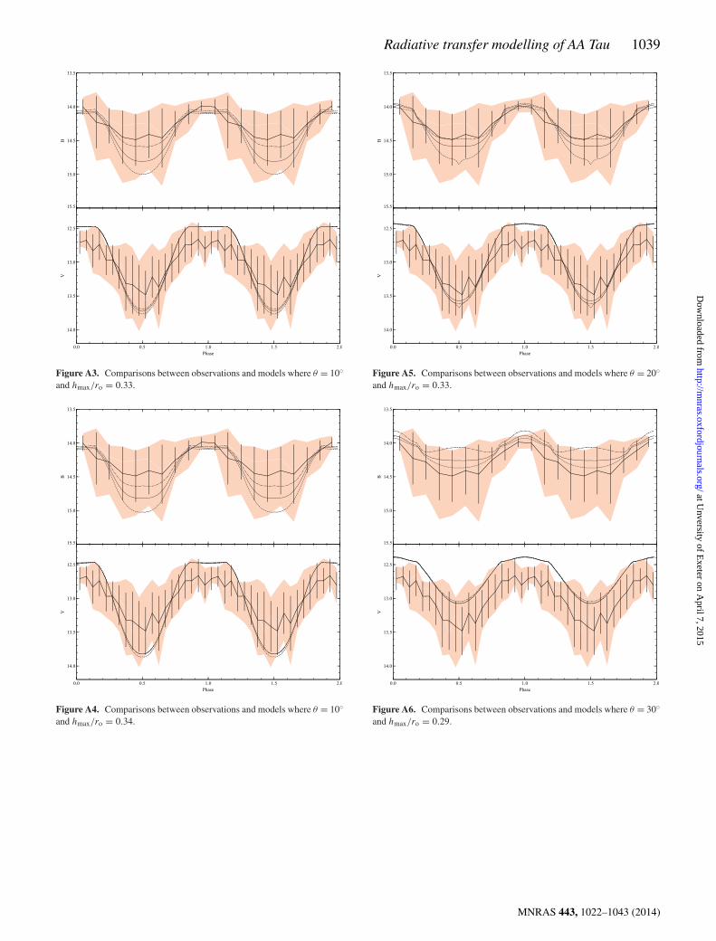
Figure A3. Comparisons between observations and models where θ = 10◦and hmax/ro = 0.33.
Figure A4. Comparisons between observations and models where θ = 10◦and hmax/ro = 0.34.
Figure A5. Comparisons between observations and models where θ = 20◦and hmax/ro = 0.33.
Figure A6. Comparisons between observations and models where θ = 30◦and hmax/ro = 0.29.
MNRAS 443, 1022–1043 (2014)
at Unversity of E
xeter on April 7, 2015
http://mnras.oxfordjournals.org/
Dow
nloaded from
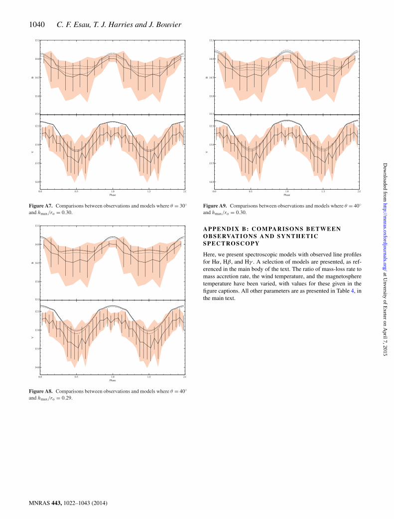
1040 C. F. Esau, T. J. Harries and J. Bouvier
Figure A7. Comparisons between observations and models where θ = 30◦and hmax/ro = 0.30.
Figure A8. Comparisons between observations and models where θ = 40◦and hmax/ro = 0.29.
Figure A9. Comparisons between observations and models where θ = 40◦and hmax/ro = 0.30.
A P P E N D I X B : C O M PA R I S O N S B E T W E E NO B S E RVAT I O N S A N D S Y N T H E T I CSPECTROSCOPY
Here, we present spectroscopic models with observed line profilesfor Hα, Hβ, and Hγ . A selection of models are presented, as ref-erenced in the main body of the text. The ratio of mass-loss rate tomass accretion rate, the wind temperature, and the magnetospheretemperature have been varied, with values for these given in thefigure captions. All other parameters are as presented in Table 4, inthe main text.
MNRAS 443, 1022–1043 (2014)
at Unversity of E
xeter on April 7, 2015
http://mnras.oxfordjournals.org/
Dow
nloaded from
Radiative transfer modelling of AA Tau 1041
Figure B1. Comparison of models with observed line profiles for Mwind/Macc = 0.1, Tmag = 8900 K and Twind = 8000 K. The magnetosphere contributionis shown by the red dotted line.
(a) Hα (b) Hγ
Figure B2. Comparison of models with observed line profiles for Mwind/Macc = 0.09, Tmag = 8500 K and Twind = 8000 K for Hα and Hγ . The magnetospherecontribution is shown by the red dotted line.
MNRAS 443, 1022–1043 (2014)
at Unversity of E
xeter on April 7, 2015
http://mnras.oxfordjournals.org/
Dow
nloaded from
1042 C. F. Esau, T. J. Harries and J. Bouvier
Figure B3. Observed Hα, Hβ, and Hγ profiles compared with models where Mwind/Macc = 0.10, Tmag = 8500 K and Twind = 7900 K. The magnetospherecontribution is shown by the red dotted line.
MNRAS 443, 1022–1043 (2014)
at Unversity of E
xeter on April 7, 2015
http://mnras.oxfordjournals.org/
Dow
nloaded from
Radiative transfer modelling of AA Tau 1043
Figure B4. Observed Hα, Hβ, and Hγ profiles compared with models where Mwind/Macc = 0.10, Tmag = 8400 K and Twind = 8000 K. The magnetospherecontribution is shown by the red dotted line.
This paper has been typeset from a TEX/LATEX file prepared by the author.
MNRAS 443, 1022–1043 (2014)
at Unversity of E
xeter on April 7, 2015
http://mnras.oxfordjournals.org/
Dow
nloaded from