An approach to correct the effects of phytoplankton verticalnonuniform distribution on remote sensing reflectance ofcyanobacterial bloom waters

Kun Xue, Yuchao Zhang, Ronghua Ma,* Hongtao DuanKey Laboratory of Watershed Geographic Sciences, Nanjing Institute of Geography and Limnology, Chinese Academy ofSciences, Nanjing 210008, China

Abstract

Cyanobacterial blooms occur frequently in eutrophic lakes and their potentially harmful effects affected

the security of drinking water and food sources, biodiversity, and economic activities, and attracted the

attention of general public worldwide. Cyanobacteria could move vertically in the water column by regulat-

ing their buoyancy, which leads to the assumption of homogeneous water invalid. Ecolight, based on radia-

tive transfer theory, was applied to examine the effects of vertical nonuniform of chlorophyll a

concentrations (Chl a(z)) on remote sensing reflectance spectrum (Rrs(k)) of optically complex inland waters.

Simulations for nonuniform water consisting of three Chl a(z) profile classes, including Gaussian, exponen-

tial, and power, were compared with simulations for a reference homogeneous water whose Chl a was identi-

cal to average value of the nonuniform case. The near-surface aggregation of phytoplankton are shown to

have significant influence on Rrs(k) and Chl a inversion algorithms. Variations of DRrs(k) (relative difference

of Rrs(k) between inhomogeneous and homogeneous waters with same average Chl a concentration) mainly

depended on the Chl a(z) structure parameters and wavelength. A correction scheme was developed based on

the relationships between DRrs(k) and Chl a(z) structure parameters. With knowledge of Chl a(z) profile

parameters, Rrs(k) of inhomogeneous waters can be corrected to the Rrs(k) of uniform waters with same aver-

age Chl a across the water column. Examples of field data from Lake Chaohu illustrated the effects of phyto-

plankton variation on the near infrared-to-red ratio of Rrs and the Rrs correction performance.

Eutrophication of lakes has been a major environmental

and social-economic problem across the world. The

increased intensity of cyanobacterial blooms has affected the

security of drinking water and food sources, biodiversity,

and economic activities. The optical properties of these

waters are determined by the amount of optically active con-

stituents (OACs) like phytoplankton (usually measured as

concentration of chlorophyll a, Chl a), suspended particulate

matter (SPM), and colored dissolved organic matter (CDOM).

In optically complex waters, commonly regard as Case II

waters (Morel and Prieur 1977), large part of the suspended

particulate inorganic matter (SPIM) and CDOM originates

from the inflow rivers and bottom resuspension. As a result,

concentrations of these substances vary a broad range (more

than one order of magnitude), and may not covary with Chl

a as in Case I waters (Gholamalifard et al. 2013).

Remote sensing technology has often been used to estimate

the optical properties, such as the absorption and backscatter-

ing coefficients (Loisel and Stramski 2000; Lee et al. 2002),

and determine key OACs, such as Chl a (Duan et al. 2010;

Song et al. 2013b), SPM (He et al. 2013), and phycocyanin

(Duan et al. 2012; Song et al. 2013a). It is also utilized to

detect the extent and frequency of cyanobacterial blooms

(Kutser et al. 2006; Odermatt et al. 2012; Bresciani et al. 2014;

Zhang et al. 2015). These applications of water color remote

sensing usually assume that the OACs and their correspond-

ing water inherent optical properties (IOPs) are vertically uni-

form. However, OACs of natural waters often show significant

vertical variations, which could result in vertical nonuniform

of IOPs (Andr�e 1992; Nanu and Robertson 1993; Forget et al.

2001). The observed remote sensing reflectance (Rrs(k)) con-

tains information about the optical properties within the pen-

etration depth, at which the downwelling irradiance (Ed) is

reduced to 1=e of its surface value (Gordon and Mccluney

1975). Vertical inhomogeneity of phytoplankton creates a

challenge to the usage of chlorophyll a concentration inver-

sion algorithm and determination of phytoplankton biomass

in the water column (Silulwane et al. 2010).

The vertical profiles of phytoplankton are mainly gov-

erned by meteorological, biological, and hydrological*Correspondence: rhma@niglas.ac.cn

1

LIMNOLOGYand

OCEANOGRAPHY: METHODS Limnol. Oceanogr.: Methods 00, 2017, 00–00VC 2017 Association for the Sciences of Limnology and Oceanography

doi: 10.1002/lom3.10158

conditions (Cao et al. 2006). Gaussian or shifted Gaussian

models (Mill�an-N�u~nez et al. 1997; Odermatt et al. 2012;

Bresciani et al. 2014) have been used to represent the vertical

profile of Chl a(z) in marine environments. The maximum

Chl a of Gaussian model was regarded as a common feature

of Chl a vertical distribution in these waters (Cullen and

Eppley 1981). In coastal waters or inland lakes, discharge

from rivers or terrestrial runoff may cause the vertical vari-

ability in the upper layer of the water column (Yang et al.

2013). In cyanobacterial bloom waters, cyanobacteria, such

as Microcystis aeruginosa, could regulate their buoyancy, and

move vertically in the water column due to changes of tem-

perature (Tsujimura et al. 2000), light intensity (Walsby and

Booker 1980), and nutrients (Klemer et al. 1982; Kromkamp

et al. 1989). There were few in situ datasets of vertical pro-

files of Chl a concentration in cyanobacterial bloom lakes

(Kutser et al. 2008). Four Chl a vertical profile classes, includ-

ing vertically uniform, Gaussian, exponential, and power

class, were measured in Lake Chaohu, a shallow eutrophic

lake of China (Xue et al. 2015). The Gaussian distribution of

phytoplankton measured in Lake Chaohu had maximum

Chl a value at water surface. In appropriate situations, cya-

nobacteria may float to water surface and form dense sub-

surface accumulations, which could produce extreme high

concentrations of Chl a (Wynne et al. 2010). These situa-

tions usually belong to exponential or power type of Chl a

vertical profiles, whose Chl a concentration decreased dra-

matically with water depth (Xue et al. 2015). In addition,

the typical shape of the chlorophyll a profile is often

assumed to be stable in a given region or season (Hidalgo-

Gonzalez and Alvarez-Borrego 2001). However, some studies

indicated that the vertical profile class of phytoplankton of

lakes change rapidly (D’Alimonte et al. 2014).

Several previous studies have focused on the vertical dis-

tribution of phytoplankton (Morel and Berthon 1989;

Mill�an-N�u~nez et al. 1997) and its effects on remote sensing

reflectance (Tsujimura et al. 2000; Stramska and Stramski

2005; Kutser et al. 2008). It has been demonstrated that the

vertical variations of phytoplankton have significant influ-

ence on the remote sensing reflectance in oceanic waters

(Stramska and Stramski 2005) and cyanobacterial bloom

waters (Kutser et al. 2008). In the Chl a inversion algorithms,

the relationships between Chl a and band ratio or combina-

tion of Rrs(k) were also affected by the vertical profiles of

phytoplankton (Stramska and Stramski 2005). The reality is

that the present empirical Chl a inversion algorithms are

affected to an unknown degree by the nonuniform of Chl

a(z) profiles or IOPs(z) of the water column.

Gordon and Clark (1980) proposed a hypothesis that the

Rrs(k) of vertical inhomogeneous waters is equal to the Rrs(k)

of homogeneous waters in which the Chl a is a weighted

average of the actual Chl a(z) profile within the penetration

depth. This hypothesis was accepted and used widely in

research on vertically nonuniform waters (Mill�an-N�u~nez

et al. 1997; Zaneveld et al. 2005; Bresciani et al. 2014). How-

ever, a common view concerning a reliable model for

weighted mean pigment concentration detectable by remote

sensors has not yet been achieved even for Case 1 waters

(Sokoletsky and Yacobi 2011).

In this study, we explored the effects of vertical profiles of

phytoplankton on remote sensing reflectance Rrs(k) in cyano-

bacterial bloom waters, Lake Chaohu in China. This lake is

characterized by frequent occurrence of algal blooms, and its

SPIM and CDOM are optically important, and do not covary

with Chl a. Radiative transfer simulations for inhomoge-

neous Chl a(z) profiles of three classes, including Gaussian,

exponential, and power distribution, were analyzed com-

pared with reference simulations of a homogeneous water

whose Chl a was the average value of the Chl a(z) profiles.

We aim to: (1) examine the effects of nonuniform Chl a(z)

profiles on spectral remote sensing reflectance Rrs(k) and Chl

a inversion algorithm, using dataset of radiative transfer sim-

ulations; (2) build the relationships between DRrs(k) and

structure parameters of Chl a(z) profiles; (3) convert Rrs(k) of

Chl a(z) inhomogeneous waters to corrected Rrs(k) of uni-

form waters with same average Chl a in the water column.

This is an attempt to estimate to what extent the inhomoge-

neous Chl a(z) profile might affect the remote sensing reflec-

tance and performance of the Chl a inversion algorithms

based on the vertical uniform assumption.

Data and method

Field and laboratory measurements

Lake Chaohu is the 5th largest freshwater lake in China

with a mean depth of 3.0 m and an area of 770 km2 (31825’–

31843’ N, 117817’–117851’ E, Fig. 1) (Chen et al. 2013). The

diversity of phytoplankton, including Chlorophyta, Bacillario-

phyta, Cyanophyta, Cryptophyta, and Euglenuphyta, varies sea-

sonally in Lake Chaohu. Cyanophyta has the highest average

annual density (> 90%) in comparison with other phyto-

plankton species (Yu 2010). Three field surveys were carried

out in 2013 (May 28, July 19–24, and October 10–12) to

measure concentrations of OACs, absorption coefficients,

backscattering coefficients, and remote sensing reflectance.

In each station, water samples at different depths (surface,

0.1 m, 0.2 m, 0.4 m, 0.7 m, 1.0 m, 1.5 m, 2.0 m, and 3.0 m)

were collected using an ad hoc vertical water collection

device (Xue et al. 2015).

The water samples were filtered with Whatman GF/C

glass-fibre filters (pore size of 1.2 lm), and 90% acetone

extraction was used to extract pigments. Shimadzu (Kyoto,

Japan) UV-2600 spectrophotometer was used to measure

absorbance at 630 nm, 645 nm, 663 nm, and 750 nm, and

then Chl a concentration was calculated (Ma et al. 2006).

For SPM concentrations, Whatman GF/F glass fiber filters

(pore size of 0.7 lm) were pre-combusted at 4508C for 6 h

and pre-weighted. The filters were used to filter water

Xue et al. Phytoplankton vertical nonuniform distribution

2

samples, and then were dried at 1058C for 4–6 h. SPIM (Table

1) was derived gravimetrically by burning organic matter

from the filters at 4508C for 6 h (Duan et al. 2012). The

absorption coefficients of the total particulate matter, phyto-

plankton pigments, and non-algae particulate (NAP) were

determined using the quantitative filter technique (Mitchell

1990) with GF/F glass fiber filters and a Shimadzu UV2600

spectrophotometer from 350 nm to 800 nm with 1 nm inter-

val. The baseline was corrected using a blank filter wetted

with filtered water (Ma et al. 2006). The absorbance spectra

were corrected for path length amplification (Cleveland and

Weidemann 1993) and background by subtracting the aver-

age absorbance at 750 nm from the entire spectra (Ma et al.

2006; Zhang et al. 2007). CDOM absorption (ag(k)) was

determined from filtered water (Millipore filter with 0.22 lm

pore size) using Shimadzu UV2600 spectrophotometer with

Milli-Q water as the reference and ranged from 280 nm to

700 nm with 1 nm interval. Absorbance at each wavelength

was baseline corrected by subtracting the absorbance at

700 nm (Bricaud et al. 1981; Ma et al. 2006; Zhou et al.

2015).

A spectral backscattering sensor, Hydroscat-6 (Washing-

ton, USA), provided backscattering measurements at wave-

lengths of 420 nm, 442 nm, 470 nm, 510 nm, 590 nm, and

700 nm, under the guidance of the manual from Hydro-

Optics, Biology & Instrumentation Laboratories (HOBI Labs

Inc 2010). All Hydroscat-6 data were examined to leave out

exceptional data and the mean of the remaining measure-

ments was calculated, and have been sigma corrected (cor-

rected for attenuation) using of laboratory measurements of

absorption coefficient, and then particulate backscattering

coefficients spectrum (bbp(k), m21) could be derived (Ma

et al. 2006). The backscattering probability of SPM was

derived using the optimization methods provided by Ma

et al. (2008). Following NASA protocols (Mueller et al. 2003),

an analytica spectra devices (ASD) field spectrometer (Field-

Spec Pro Dual VNIR, Boulder, U.S.A.) was used to obtain

remote sensing reflectance. First, total water leaving radiance

(Lsw), radiance of gray panel (Lp), and sky radiance (Lsky)

were measured using the ASD field spectrometer. The water

surface reflectance factor q depended on sky conditions,

wind speed, and solar zenith angle, and was assumed to be

Fig. 1. Study area and observation stations in Lake Chaohu, China. Field measurements of bio-optical parameters made during three cruise surveys in

28 May 2013 (N 5 9), 19–24 July 2013 (N 5 32) and 10–12 October 2013 (N 5 27).

Xue et al. Phytoplankton vertical nonuniform distribution

3

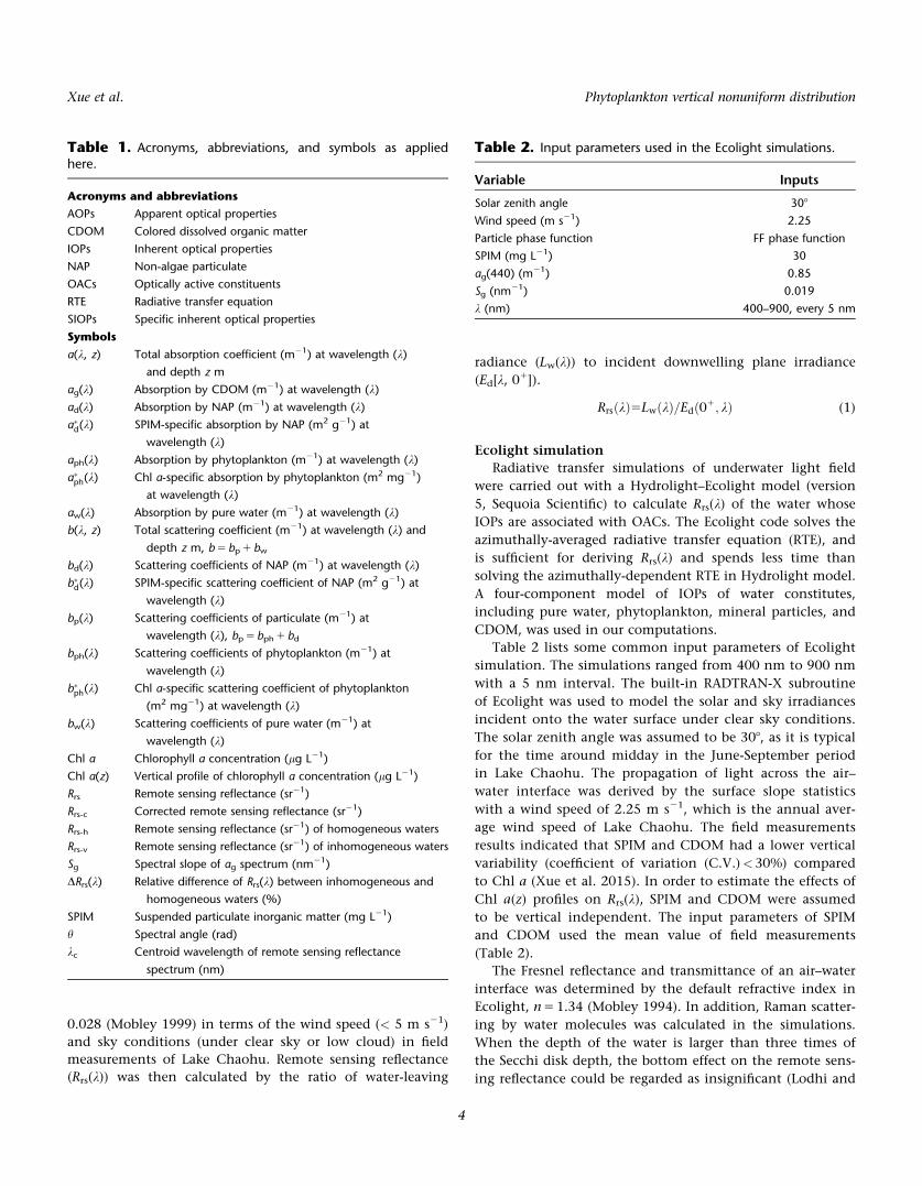
0.028 (Mobley 1999) in terms of the wind speed (< 5 m s21)

and sky conditions (under clear sky or low cloud) in field

measurements of Lake Chaohu. Remote sensing reflectance

(Rrs(k)) was then calculated by the ratio of water-leaving

radiance (Lw(k)) to incident downwelling plane irradiance

(Ed[k, 01]).

RrsðkÞ5LwðkÞ=Edð01; kÞ (1)

Ecolight simulation

Radiative transfer simulations of underwater light field

were carried out with a Hydrolight–Ecolight model (version

5, Sequoia Scientific) to calculate Rrs(k) of the water whose

IOPs are associated with OACs. The Ecolight code solves the

azimuthally-averaged radiative transfer equation (RTE), and

is sufficient for deriving Rrs(k) and spends less time than

solving the azimuthally-dependent RTE in Hydrolight model.

A four-component model of IOPs of water constitutes,

including pure water, phytoplankton, mineral particles, and

CDOM, was used in our computations.

Table 2 lists some common input parameters of Ecolight

simulation. The simulations ranged from 400 nm to 900 nm

with a 5 nm interval. The built-in RADTRAN-X subroutine

of Ecolight was used to model the solar and sky irradiances

incident onto the water surface under clear sky conditions.

The solar zenith angle was assumed to be 308, as it is typical

for the time around midday in the June-September period

in Lake Chaohu. The propagation of light across the air–

water interface was derived by the surface slope statistics

with a wind speed of 2.25 m s21, which is the annual aver-

age wind speed of Lake Chaohu. The field measurements

results indicated that SPIM and CDOM had a lower vertical

variability (coefficient of variation (C.V.)<30%) compared

to Chl a (Xue et al. 2015). In order to estimate the effects of

Chl a(z) profiles on Rrs(k), SPIM and CDOM were assumed

to be vertical independent. The input parameters of SPIM

and CDOM used the mean value of field measurements

(Table 2).

The Fresnel reflectance and transmittance of an air–water

interface was determined by the default refractive index in

Ecolight, n 5 1.34 (Mobley 1994). In addition, Raman scatter-

ing by water molecules was calculated in the simulations.

When the depth of the water is larger than three times of

the Secchi disk depth, the bottom effect on the remote sens-

ing reflectance could be regarded as insignificant (Lodhi and

Table 1. Acronyms, abbreviations, and symbols as appliedhere.

Acronyms and abbreviations

AOPs Apparent optical properties

CDOM Colored dissolved organic matter

IOPs Inherent optical properties

NAP Non-algae particulate

OACs Optically active constituents

RTE Radiative transfer equation

SIOPs Specific inherent optical properties

Symbols

a(k, z) Total absorption coefficient (m21) at wavelength (k)

and depth z m

ag(k) Absorption by CDOM (m21) at wavelength (k)

ad(k) Absorption by NAP (m21) at wavelength (k)

a�d(k) SPIM-specific absorption by NAP (m2 g21) at

wavelength (k)

aph(k) Absorption by phytoplankton (m21) at wavelength (k)

a�ph(k) Chl a-specific absorption by phytoplankton (m2 mg21)

at wavelength (k)

aw(k) Absorption by pure water (m21) at wavelength (k)

b(k, z) Total scattering coefficient (m21) at wavelength (k) and

depth z m, b 5 bp 1 bw

bd(k) Scattering coefficients of NAP (m21) at wavelength (k)

b�d(k) SPIM-specific scattering coefficient of NAP (m2 g21) at

wavelength (k)

bp(k) Scattering coefficients of particulate (m21) at

wavelength (k), bp 5 bph 1 bd

bph(k) Scattering coefficients of phytoplankton (m21) at

wavelength (k)

b�ph(k) Chl a-specific scattering coefficient of phytoplankton

(m2 mg21) at wavelength (k)

bw(k) Scattering coefficients of pure water (m21) at

wavelength (k)

Chl a Chlorophyll a concentration (lg L21)

Chl a(z) Vertical profile of chlorophyll a concentration (lg L21)

Rrs Remote sensing reflectance (sr21)

Rrs-c Corrected remote sensing reflectance (sr21)

Rrs-h Remote sensing reflectance (sr21) of homogeneous waters

Rrs-v Remote sensing reflectance (sr21) of inhomogeneous waters

Sg Spectral slope of ag spectrum (nm21)

DRrs(k) Relative difference of Rrs(k) between inhomogeneous and

homogeneous waters (%)

SPIM Suspended particulate inorganic matter (mg L21)

h Spectral angle (rad)

kc Centroid wavelength of remote sensing reflectance

spectrum (nm)

Table 2. Input parameters used in the Ecolight simulations.

Variable Inputs

Solar zenith angle 308

Wind speed (m s21) 2.25

Particle phase function FF phase function

SPIM (mg L21) 30

ag(440) (m21) 0.85

Sg (nm21) 0.019

k (nm) 400–900, every 5 nm

Xue et al. Phytoplankton vertical nonuniform distribution

4

Rundquist 2001). Thus, water bottom reflection of Lake

Chaohu was ignored (Ma et al. 2006; Ma et al. 2011a; Ma

et al. 2011b).

Inherent optical properties

In the four-component model, total spectral absorption

coefficient of water, a(k, z) (m21), is expressed as:

aðk; zÞ5awðkÞ1aphðk; zÞ1adðkÞ1agðkÞ (2)

where a(k, z) is the spectral absorption coefficient of water at

wavelength k nm and depth z m. aph(k, z) is the spectral

absorption coefficient of phytoplankton at k nm and z m.

aw(k) (Pope and Fry 1997), ad(k), and ag(k) are the spectral

absorption coefficient of pure water, NAP, and CDOM at knm, and were assumed to be independent in depth in this

study. The vertical profile of aph(k, z) is calculated from:

aphðk; zÞ5Chl aðzÞ3a�phðkÞ (3)

where a�ph(k) (m2 mg21) is the spectral Chl a-specific absorp-

tion coefficient of phytoplankton, and is assumed to be con-

stant with depth. The NAP absorption is calculated from:

adðkÞ5SPIM3a�dðkÞ (4)

where a�d(k) (m2 g21) is the spectral SPIM-specific absorption

coefficient of SPIM. The CDOM absorption is modeled as an

exponential function of light wavelength:

agðkÞ5agðk0Þexp ½2Sgðk2k0Þ� (5)

where ag(k0) is the CDOM absorption coefficient estimated

at a reference wavelength k0 (5 440 nm), and Sg (nm21) is

the spectral slope of the CDOM absorption spectrum

between 400 nm and 700 nm. Following the in situ measure-

ments, Sg ranged from 0.012 nm21 to 0.043 nm21 with aver-

age of 0.019 (6 0.004) nm21.

The total spectral scattering coefficient, b(k, z)(m21), is

the sum of scattering coefficient of pure water, bw(k) (m21)

(Morel 1974), and SPM, bp(k, z) (m21):

bðk; zÞ5bwðk; zÞ1bpðk; zÞ (6)

bp(k, z) is the sum of scattering coefficient of phytoplankton,

bph(k) (m21), and NAP, bd(k) (m21):

bpðk; zÞ5bphðk; zÞ1bdðk; zÞ (7)

b�ph(k) (m2 mg21) and b�d(k) (m2 g21) are the spectral specific

scattering coefficient of phytoplankton and NAP. b�ph(k) and

b�d(k) were determined by partitioning the bbp into scattering

coefficient of phytoplankton and NAP (Eq. 7) using multiple

linear regression with Chl a and SPIM concentration (Eq. 8)

(Snyder et al. 2008):

bpðk; zÞ5Chl aðzÞ3b�phðkÞ1SPIM3b�dðkÞ (8)

Similarly to mass specific absorption coefficient, the values

of b�ph(k) and b�d(k) were assumed to be independent of

depth.

The specific inherent optical properties (SIOPs) of Lake

Chaohu were derived from the field measurements, and then

IOPs could be derived based on the above Eqs. 2–-8. Optical

measurements of the water samples ranging from 350 nm to

800 nm were extrapolate to 900 nm in the near infrared

(NIR) part of the spectrum. Typical examples of specific

absorption and backscattering coefficient spectra of Lake

Chaohu were set as the input files of Ecolight simulation

(Fig. 2).

The scattering phase functions for pure water, phyto-

plankton, and mineral particles were also key input IOPs.

The scattering phase function of pure water was provided by

the file (pureh2o.dpf) in the Ecolight model. The Fournier-

Fig. 2. Average SIOPs for Lake Chaohu: (a) the spectral absorptioncoefficient of pure water (aw, m21) and the specific absorption coeffi-cient spectra of Chl a (aph*, m2 mg21), NAP (ad*, m2 g21) and CDOM

(ag*, dimensionless); (b) the spectral backscattering coefficient of purewater (bbw, m21) and the specific backscattering coefficient spectra of

Chl a (bbph*, m2 mg21), NAP (bbd*, m2 g21). aw(k) and bw(k) are readfrom file HE5\data\H20abDefaults.txt in Hydrolight-Ecolight model.

Xue et al. Phytoplankton vertical nonuniform distribution

5

Forand (FF) phase function (Fournier and Forand 1994) was

specified as the scattering phase function of phytoplankton

and NAP (Mobley et al. 2002). FF phase function can be

determined mainly by the backscattering fraction, bb/b,

which was derived by optimization method. Ecolight simu-

lation was performed by changing the backscattering frac-

tion of phytoplankton and NAP, and the simulation with

lowest errors between simulated Rrs(k) and field measured

Rrs(k) had optimum value of backscattering fraction. Back-

scattering fraction was 0.02 and 0.05 for the phytoplankton

and NAP, respectively. Some studies demonstrated that the

backscattering ratio is wavelength dependent and not a con-

stant value (Aas et al. 2005). The particulate backscattering

fractions and the particulate scattering phase functions were

assumed to be independent of light wavelength and depth

in this study.

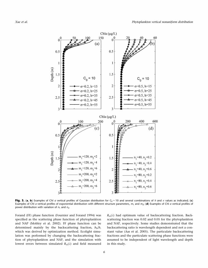
Fig. 3. (a, b) Examples of Chl a vertical profiles of Gaussian distribution for C0 5 10 and several combinations of h and r values as indicated; (c)Examples of Chl a vertical profiles of exponential distribution with different structure parameters, m1 and m2; (d) Examples of Chl a vertical profiles of

power distribution with variation of n1 and n2.

Xue et al. Phytoplankton vertical nonuniform distribution

6

Chl a(z) profiles

Previous study found that the Chl a(z) profiles of Lake

Chaohu exhibited four vertical classes, including vertical

uniform, Gaussian, exponential, and power distribution

(Xue et al. 2015). These inhomogeneous vertical Chl a(z)

profiles usually had maximum concentration at the water

surface in cyanobacterial bloom waters. Specifically, Chl

a(z) profiles of the three inhomogeneous profile classes

were derived according to the range and step of vertical

structure parameters of each class, which is derived from

field measurements (Eqs. 9–-11; Fig. 3). Based on the range

and step of structure parameters as presented in Table 3,

1008, 2400, and 576 profiles of Chl a(z) were generated for

Gaussian, exponential, and power class, respectively.

Hence, total of 3984 radiative transfer simulations were

made with different sets of input IOPs representing nonuni-

form water column.

Chl aGðzÞ5C01h

rffiffiffiffiffiffi2pp exp

�2

1

2ðzrÞ2�

(9)

Chl aEðzÞ5m13exp ðm23zÞ (10)

Chl aPðzÞ5n13zn2 (11)

In addition to the simulations of vertical inhomogeneous

water, reference simulations for vertically homogeneous

water were also performed. In the reference simulation, the

average Chl a of the corresponding inhomogeneous case was

used to determine the independent IOPs. These reference

simulations examined the effects of vertical Chl a(z) profiles

on Rrs(k) relative to the vertically homogeneous water. For

each of 3984 simulations of nonuniform water, the relative

difference (DRrs(k)) between Rrs(k) for the nonuniform case

and Rrs(k) for the corresponding uniform case was calculated

as:

DRrsðkÞ5Rrs2vðkÞ2Rrs2hðkÞ

Rrs2hðkÞ3100% (12)

where Rrs-v(k) and Rrs-h(k) was the spectral Rrs(k) of the verti-

cally nonuniform and uniform water, respectively. DRrs(k)

was used to analyze the sensitivity of Rrs(k) to Chl a(z) pro-

files within the water column.

Method to correct Rrs(k) of nonuniform waters

Rrs-v(k) contains information of Chl a(z) profiles, but it is

difficult to decide to what extent Rrs(k) is depended on verti-

cal effects. A Rrs(k) correction scheme was developed to solve

this problem and decreased the influence of vertical distribu-

tion of Chl a(z) on Rrs(k) based on the relationships between

DRrs(k) and Chl a(z) structure parameters. According to Eq.

12, Rrs-v(k) can be converted to Rrs-h(k), if DRrs(k) could be

estimated. First, as DRrs(k) varies with structure parameters of

Chl a(z) (S), empirical relationships between DRrs(k) and Chl

a(z) profile parameters of three Chl a(z) profile classes were

build. Then, corrected Rrs(k) (Rrs-c(k)) could be derived

according to Eq. 13:

Rrs2ciðkÞ5Rrs2viðkÞ

DRrs2iðkÞ=10011(13)

Hence, the corrected Rrs(k) of each Chl a profile class, Rrs-

ci(k), would be derived using the Rrs-vi(k) and structure

parameters of Chl a(z), Si. i 5 1, 2, 3, represents Gaussian,

exponential, and power class, respectively.

Statistical analyses

To exhibit the variability of Chl a(z) vertical profiles, the

C.V. was derived with the ratio of standard deviation (SD)

and mean value:

CV5SD

mean3100% (14)

Centroid wavelength of remote sensing reflectance spectrum

(kc) was used to present the difference of centroid wave-

length as Chl a(z) profiles changed. It was calculated as (Lin

et al. 2012):

kc5

X900

k5400

k3RrsðkÞ

X900

k5400

RrsðkÞ(15)

Spectral angle (h) measures differences between Rrs(k) of ver-

tical uniform and nonuniform waters in spectral shape, and

is calculated as (Kruse et al. 1993; Dennison et al. 2004):

h5cos 21

X900

k5400

Rrs2hðkÞRrs2vðkÞffiffiffiffiffiffiffiffiffiffiffiffiffiffiffiffiffiffiffiffiffiffiffiffiffiffiffiffiffiffiffiX900

k5400

Rrs2h2ðkÞ

vuutffiffiffiffiffiffiffiffiffiffiffiffiffiffiffiffiffiffiffiffiffiffiffiffiffiffiffiffiffiffiX900

k5400

Rrs2v2ðkÞ

vuut

0BBBBBB@

1CCCCCCA

(16)

h ranges from 0 to p/2, h 5 0 represents that the two spec-

trum are similar, and large value illustrates large difference.

Table 3. Range and step of Chl a(z) structure parameters con-sidered in radiative transfer simulations of underwater light field.

Class Parameters Range Step Numbers

Gaussian C0 0–40 5 1008

h 1–76 5

r 0.2–1.4 0.2

Exponential m1 120–600 20 2400

m2 0.5–10 0.1

Power n1 10–80 2 576

n2 0.2–0.95 0.05

Xue et al. Phytoplankton vertical nonuniform distribution

7

R2 and root mean square error (RMSE) in log space were

used to assess algorithm performance:

R2512

XN

i51ðyi2xiÞ2XN

i51ðyi2�xiÞ2

(17)

RMSEðlog Þ5

ffiffiffiffiffiffiffiffiffiffiffiffiffiffiffiffiffiffiffiffiffiffiffiffiffiffiffiffiffiffiffiffiffiffiffiffiffiffiffiffiffiffiffiffiffiffiffiffiffiffiffiffiffiffiffiffiffiffiffiffiffiffiffiffi1

N

XNi51

ðlog 10ðyiÞ2log 10ðxiÞÞ2vuut (18)

where xi and yi refer to the referenced and modeled values of

the ith sample, N is the number of samples.

Results

Effects of Chl a vertical nonuniform on Rrs(k)

There exist many Chl a(z) vertical profiles with different

structure parameters of each vertical profile class (Gaussian,

exponential, and power class), even the average Chl a con-

centration of the water column is constant. Centroid wave-

length (kc) and spectral angle (h) reflect the general variation

of remote sensing reflectance spectrum (Fig. 4). kc represents

the centroid position of Rrs(k) spectra between 400 nm and

900 nm. h could be used to evaluate the similarity of Rrs(k)

spectra between homogeneous water and inhomogeneous

water with same average Chl a concentration in the water

column.

The relationships between kc and C.V. of Chl a(z) profiles

of different vertical profile classes showed that kc increased

with increase of C.V. among the three classes. Compared to

homogeneous waters, kc of Gaussian class moved from near

612 nm to the longer wavelength, about 660 nm (Fig. 4a).

Spectral angle (h) between homogeneous water and

inhomogeneous water had similar tendency with kc (Fig. 4b).

In addition, same C.V. was corresponding to different kc and

h in different Chl a(z) profile classes, and extent of the

effects of Chl a vertical nonuniform on Rrs(k) was different

among three classes, in which the Gaussian class was more

sensitive than other two classes. Thus, we analyzed the

effects of Chl a vertical nonuniform on Rrs(k) of each class

separately in the following content.

When the average Chl a concentration of the water col-

umn is unchangeable, Rrs(k) spectra of inhomogeneous Chl

a(z) profiles can depart apparently from the spectra of the

homogeneous ones. Example results of Rrs(k) and DRrs(k) sim-

ulated by Ecolight for different pairs of Chl a vertical struc-

ture parameters were provided (Fig. 5). In each class of Chl

a(z) profile, the multiple plots of Rrs(k) spectra corresponded

to different values of structure parameters.

For Gaussian class, the presence of near-surface high Chl

a value led to decrease in Rrs(k) from 400 nm to about

700 nm. Under these conditions, DRrs(k) in the green and

red wavelengths reaches the values of 240% to 260% (Fig.

5a,b). Water column stratification had reverse effect on Rrs(k)

and enhanced the Rrs(k) at wavelength longer than 700 nm.

These departures were most obvious for high contrast in Chl

a(z) profiles. For example, DRrs(k) reached 260% in the red

and 70% in the NIR spectrum when the top layer was very

thin, i.e., r 5 0.2 (Fig. 5a). The increase in C0 naturally

resulted in reduction of the observed effects due to weak

stratification. For large C0 values (e.g., C0 5 40 in Fig. 5c,d),

the magnitude of Rrs-v(k) was close to that of Rrs-h(k) from

400 nm to 900 nm.

The simulations for exponential class also showed that

the largest difference was observed at about 600–700 nm

when the top layer is thin as m2 increase (Fig. 5e,f). Howev-

er, Rrs(k) had highest values in red wavelength when most of

Fig. 4. Variation of (a) centroid wavelength (kc) and (b) spectral angle (h) with C.V. of Chl a(z) profiles in Gaussian (“G”), exponential (“E”), andpower (“P”) class.

Xue et al. Phytoplankton vertical nonuniform distribution

8

Fig. 5. Example results of radiative transfer simulations of Gaussian (a–d), exponential (e, f) and power (g, h) profile classes, showing the differences inRrs(k) and DRrs(k) between the uniform water (black curves) and the inhomogeneous water (color curves). The average Chl a (Chl a_ave) in the nonuni-

form case is identical to that in the uniform case. (a, b) C0 5 10, Chl a_ave 5 45 lg L21; (c, d) r 5 0.4, Chl a_ave 5 45 lg L21; (e, f) Chl a_ave 5 60 lgL21; (g, h) Chl a_ave 5 60 lg L21. Each graph for DRrs(k) (right-hand panels) is corresponding to the data presented in the left-hand panels.

Xue et al. Phytoplankton vertical nonuniform distribution

9

the cyanobacteria were close to the water surface (Fig. 5g,h).

For instance, as the decrease of n1 for power class, the phyto-

plankton aggregated near the water surface, and Rrs(k) of Chl

a vertical nonuniform was larger than the vertical uniform

case in the visible region and lower in the NIR band. The

Rrs(k) spectra of uniformly water were significantly lower

than those of nonuniform vertical distributions with average

Chl a 60 lg L21 in the water column. This had similar results

as Kutser et al. (2008), and showed opposite tendency with

the other two profile classes.

The Chl a(z) inhomogeneous profiles not only introduced

the differences of shape and magnitude in remote sensing

reflectance spectra, but also affected remote sensing esti-

mates of Chl a concentration. Standard Chl a inversion algo-

rithms of Case I waters are based on the blue-green ratio,

and fail badly in complex inland waters. First, we made a

test using the band ratio (Rrs(709)/Rrs(675)) of simulated data

to illustrate the influence of Chl a vertical profiles on Chl a

inversion algorithm. The results indicated that correlation

between Rrs-h(709)/Rrs-h(675) and Chl a of vertical uniform

waters was good (R2 5 0.99):

x5Rrsð709Þ=Rrsð675Þ

Chl a546:29x2137:52x246:563(19)

However, the Chl a estimated by the above relationship

using Rrs-v(709)/Rrs-v(675) of nonuniform waters did not

match the homogeneous ones (Fig. 6a–c). The scatter plots

between Chl a of homogeneous water and modeled Chl a of

inhomogeneous waters based on the above equation illus-

trated that vertical inhomogeneous of Chl a(z) profiles

severely influenced the accuracy of Chl a algorithm. General-

ly, overestimation of Chl a inversion algorithm was intro-

duced, and the average relative error between Chl a-model

and Chl a–h was 79.8%, 549.9%, and 99.6% for Gaussian,

exponential, and power class, respectively. For example, sur-

face Chl a of nonuniform case ranged about 50–113 lg L21,

while the average concentration in the uniform case was

Fig. 6. Comparison between modeled Chl a and Chl a of homogeneous waters simulated by Ecolight of Gaussian (a, d), exponential (b, e), andpower (c, f) class. Modeled Chl a of (a–c) are derived by band ratio algorithm (Eq. 19), modeled Chl a of (d–f) are derived by FLH inversion algo-rithm (Eq. 20). The points close to the 1:1 line represent simulations with negligible effect of inhomogeneous Chl a(z) profiles on Chl a inversion

algorithm.

Xue et al. Phytoplankton vertical nonuniform distribution

10

45 lg L21. The relative error of DRrs-v(709)/Rrs-v(675) was 14

times of DRrs(443), that is to say, when the relative error of

DRrs(443) was 10%, the error of Rrs(709)/Rrs(675) would be

140%, and the relative error of Chl a estimation raised up to

153%.

As the sensitivity of Chl a algorithm to Rrs variation was

different, another Chl a algorithm developed based on fluo-

rescence line height (FLH) index (Letelier and Abbott 1996)

was used to estimate the effect of Chl a vertical nonuniform

on Chl a inversion:

Fig. 7. Dependence of relative difference between inhomogeneous and homogeneous waters of Rrs (DRrs) on Chl a vertical structure parameters at

443 nm, 550 nm, 675 nm, and 709 nm. C0 is given to be 10 in the 1st column, and h is 40 in the 2nd column.

Xue et al. Phytoplankton vertical nonuniform distribution

11

FLH5Rrs k2ð Þ2 Rrs k1ð Þ1 Rrs k3ð Þ2Rrs k1ð Þð Þ k22k1

k32k1

� �

Chl a538:89EXPð2359:9FLHÞ(20)

where, k1 5 665 nm, k2 5 681 nm, k3 5 709 nm, R2 5 0.99. In

this model, the average relative error between Chl a-model

and Chl a–h was 140%, 508%, and 92% for Gaussian, expo-

nential, and power class, respectively. Most data points of

the nonuniform Chl a(z) profiles lie on the left-hand side of

1:1 line or 1:2 line (Fig. 6d–f). It indicated that application

of the band ratio or FLH algorithm can lead to substantial

overestimation of surface Chl a, if the vertical variation of

phytoplankton in cyanobacterial bloom waters was ignored.

Relationships of DRrs(k) and Chl a structure parameters

The relationships between relative difference of remote

sensing reflectance (DRrs(k)) and Chl a vertical structure

parameters were illustrated for the three inhomogeneous Chl

a vertical profile classes (Fig. 7). For Gaussian class, when h

increased or r decreased, the variation of Chl a(z) profile

within the Chl a peak increased, and then DRrs(k) increased

as well. The effect of Chl a(z) profile on Rrs(k) weakened with

the increase of r. For r 5 0.2 and h 5 40, Rrs-v(443) was lower

by � 20%, Rrs-v(550) was lower by 30% than the uniform

ones. If the Chl a peak was wide (r 5 0.8, h 5 40), DRrs(550)

was about 210%. For exponential profile class, DRrs increased

with increase of m1 and decrease of m2. Variation of m2 had

little influence on DRrs, especially when m2 was large. For

power profile class, n2 had significant effect on DRrs, and var-

iation of DRrs was less than 10% with the increase of n1 from

10 to 80.

Structure parameters of different Chl a profile classes have

important influence on DRrs(k). Figures 5 and 7 showed sev-

eral examples of the effects caused by changing structure

parameters of the Chl a(z) profile. Based on about 3/4 of the

simulated data (N 5 2874), we established a relationship

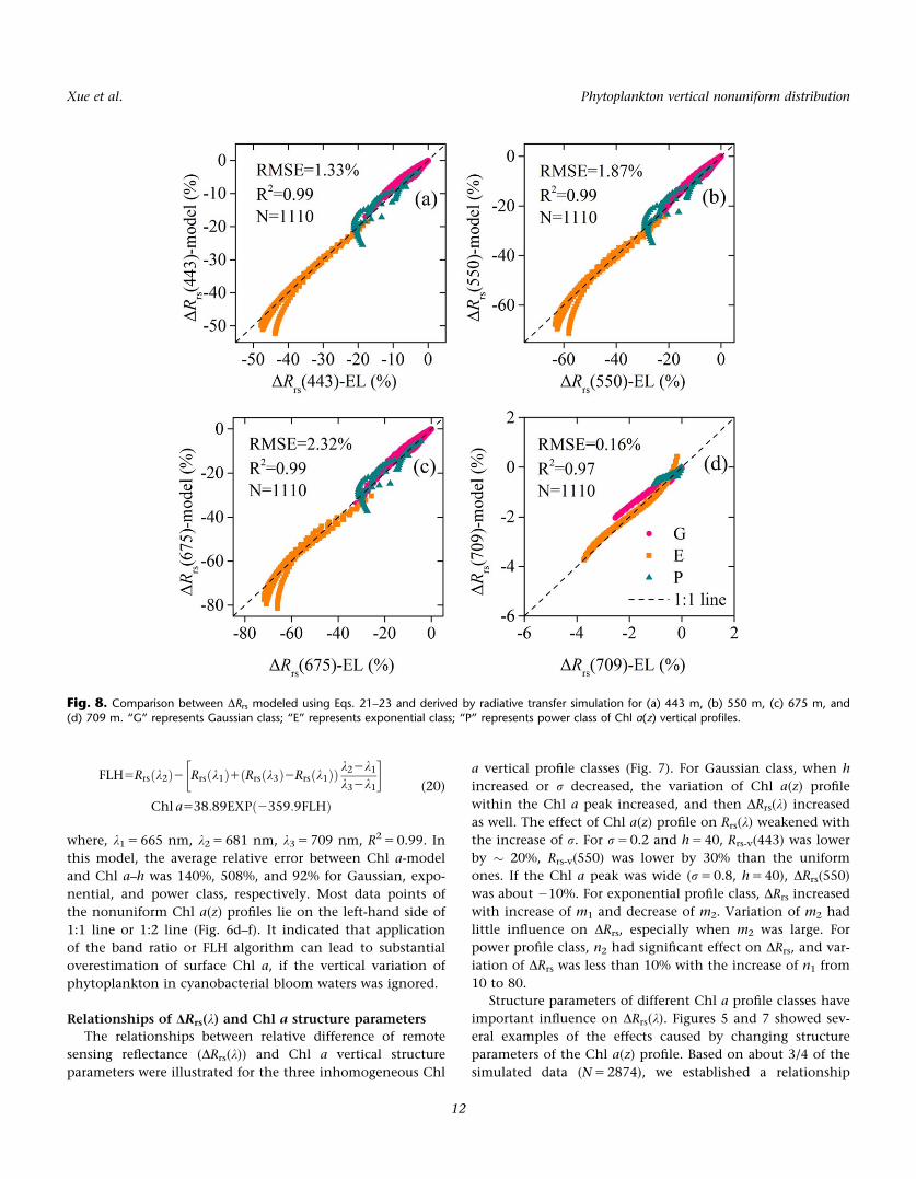
Fig. 8. Comparison between DRrs modeled using Eqs. 21–23 and derived by radiative transfer simulation for (a) 443 m, (b) 550 m, (c) 675 m, and(d) 709 m. “G” represents Gaussian class; “E” represents exponential class; “P” represents power class of Chl a(z) vertical profiles.

Xue et al. Phytoplankton vertical nonuniform distribution

12

between DRrs(k) and Chl a(z) structure parameters for each

Chl a(z) profile class to illustrate the effects quantitatively:

DRrs21ðkÞ5A1ðkÞh

rC01A2ðkÞ

h

r(21)

DRrs22ðkÞ5B1ðkÞln ðm1Þ1B2ðkÞm21B3ðkÞ (22)

DRrs23ðkÞ5C1ðkÞn11C2ðkÞn21C3ðkÞ (23)

where DRrs-i(k) (i 5 1, 2, 3) represents DRrs(k) of Gaussian,

exponential, and power profile class of Chl a(z). S1 (5 [A1,

A2]), S2 (5 [B1, B2, B3]), and S3 (5 [C1, C2, C3]) were model

parameters of each Chl a profile class. Performance of the

above equations of four bands, including 443 nm, 550 nm,

675 nm, and 709 nm was validated by the rest of the data

(N 5 1110). The results showed that average RMSE of each

wavelength was 1.33%, 1.87%, 2.32%, and 0.16% with

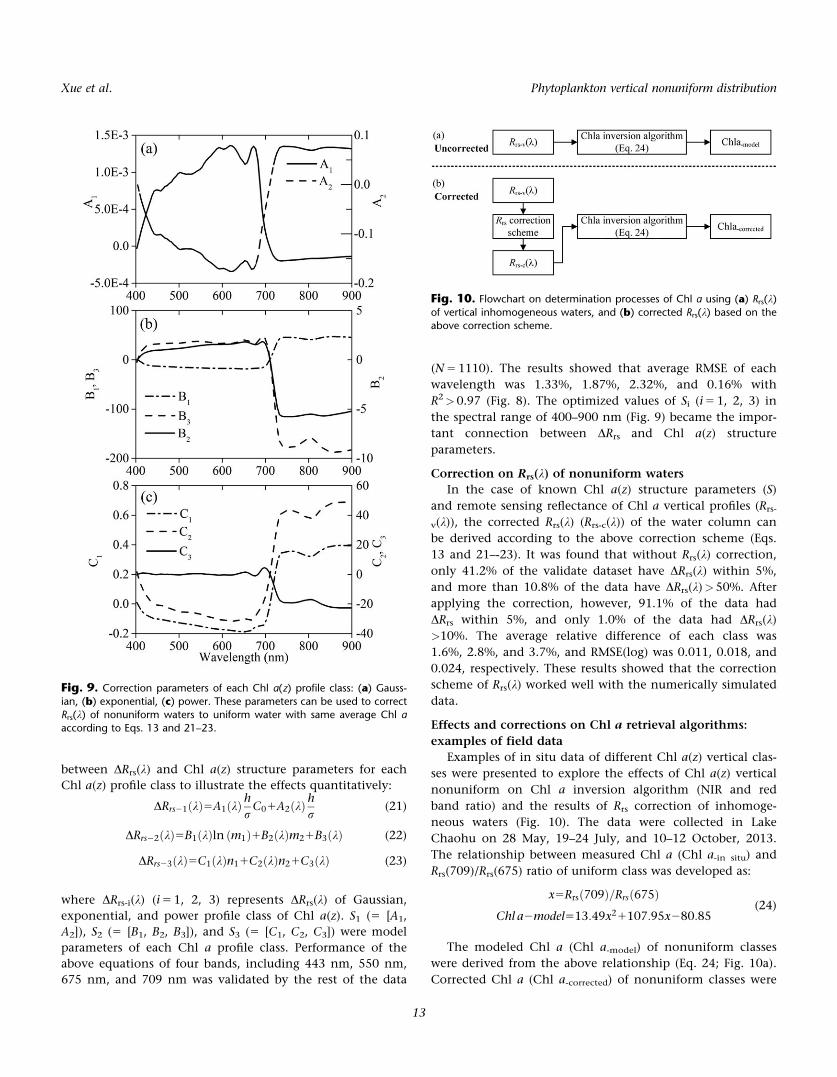
R2>0.97 (Fig. 8). The optimized values of Si (i 5 1, 2, 3) in

the spectral range of 400–900 nm (Fig. 9) became the impor-

tant connection between DRrs and Chl a(z) structure

parameters.

Correction on Rrs(k) of nonuniform waters

In the case of known Chl a(z) structure parameters (S)

and remote sensing reflectance of Chl a vertical profiles (Rrs-

v(k)), the corrected Rrs(k) (Rrs-c(k)) of the water column can

be derived according to the above correction scheme (Eqs.

13 and 21–-23). It was found that without Rrs(k) correction,

only 41.2% of the validate dataset have DRrs(k) within 5%,

and more than 10.8% of the data have DRrs(k)>50%. After

applying the correction, however, 91.1% of the data had

DRrs within 5%, and only 1.0% of the data had DRrs(k)

>10%. The average relative difference of each class was

1.6%, 2.8%, and 3.7%, and RMSE(log) was 0.011, 0.018, and

0.024, respectively. These results showed that the correction

scheme of Rrs(k) worked well with the numerically simulated

data.

Effects and corrections on Chl a retrieval algorithms:

examples of field data

Examples of in situ data of different Chl a(z) vertical clas-

ses were presented to explore the effects of Chl a(z) vertical

nonuniform on Chl a inversion algorithm (NIR and red

band ratio) and the results of Rrs correction of inhomoge-

neous waters (Fig. 10). The data were collected in Lake

Chaohu on 28 May, 19–24 July, and 10–12 October, 2013.

The relationship between measured Chl a (Chl a-in situ) and

Rrs(709)/Rrs(675) ratio of uniform class was developed as:

x5Rrsð709Þ=Rrsð675Þ

Chl a2model513:49x21107:95x280:85(24)

The modeled Chl a (Chl a-model) of nonuniform classes

were derived from the above relationship (Eq. 24; Fig. 10a).

Corrected Chl a (Chl a-corrected) of nonuniform classes were

Fig. 9. Correction parameters of each Chl a(z) profile class: (a) Gauss-

ian, (b) exponential, (c) power. These parameters can be used to correctRrs(k) of nonuniform waters to uniform water with same average Chl a

according to Eqs. 13 and 21–23.

Fig. 10. Flowchart on determination processes of Chl a using (a) Rrs(k)

of vertical inhomogeneous waters, and (b) corrected Rrs(k) based on theabove correction scheme.

Xue et al. Phytoplankton vertical nonuniform distribution

13

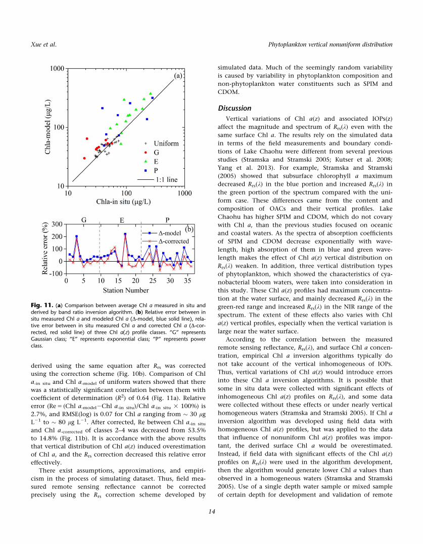
derived using the same equation after Rrs was corrected

using the correction scheme (Fig. 10b). Comparison of Chl

a-in situ and Chl a-model of uniform waters showed that there

was a statistically significant correlation between them with

coefficient of determination (R2) of 0.64 (Fig. 11a). Relative

error (Re 5 (Chl a-model2Chl a-in situ)/Chl a-in situ 3 100%) is

2.7%, and RMSE(log) is 0.07 for Chl a ranging from � 30 lg

L21 to � 80 lg L21. After corrected, Re between Chl a-in situ

and Chl a-corrected of classes 2–4 was decreased from 53.5%

to 14.8% (Fig. 11b). It is accordance with the above results

that vertical distribution of Chl a(z) induced overestimation

of Chl a, and the Rrs correction decreased this relative error

effectively.

There exist assumptions, approximations, and empiri-

cism in the process of simulating dataset. Thus, field mea-

sured remote sensing reflectance cannot be corrected

precisely using the Rrs correction scheme developed by

simulated data. Much of the seemingly random variability

is caused by variability in phytoplankton composition and

non-phytoplankton water constituents such as SPIM and

CDOM.

Discussion

Vertical variations of Chl a(z) and associated IOPs(z)

affect the magnitude and spectrum of Rrs(k) even with the

same surface Chl a. The results rely on the simulated data

in terms of the field measurements and boundary condi-

tions of Lake Chaohu were different from several previous

studies (Stramska and Stramski 2005; Kutser et al. 2008;

Yang et al. 2013). For example, Stramska and Stramski

(2005) showed that subsurface chlorophyll a maximum

decreased Rrs(k) in the blue portion and increased Rrs(k) in

the green portion of the spectrum compared with the uni-

form case. These differences came from the content and

composition of OACs and their vertical profiles. Lake

Chaohu has higher SPIM and CDOM, which do not covary

with Chl a, than the previous studies focused on oceanic

and coastal waters. As the spectra of absorption coefficients

of SPIM and CDOM decrease exponentially with wave-

length, high absorption of them in blue and green wave-

length makes the effect of Chl a(z) vertical distribution on

Rrs(k) weaken. In addition, three vertical distribution types

of phytoplankton, which showed the characteristics of cya-

nobacterial bloom waters, were taken into consideration in

this study. These Chl a(z) profiles had maximum concentra-

tion at the water surface, and mainly decreased Rrs(k) in the

green-red range and increased Rrs(k) in the NIR range of the

spectrum. The extent of these effects also varies with Chl

a(z) vertical profiles, especially when the vertical variation is

large near the water surface.

According to the correlation between the measured

remote sensing reflectance, Rrs(k), and surface Chl a concen-

tration, empirical Chl a inversion algorithms typically do

not take account of the vertical inhomogeneous of IOPs.

Thus, vertical variations of Chl a(z) would introduce errors

into these Chl a inversion algorithms. It is possible that

some in situ data were collected with significant effects of

inhomogeneous Chl a(z) profiles on Rrs(k), and some data

were collected without these effects or under nearly vertical

homogeneous waters (Stramska and Stramski 2005). If Chl a

inversion algorithm was developed using field data with

homogeneous Chl a(z) profiles, but was applied to the data

that influence of nonuniform Chl a(z) profiles was impor-

tant, the derived surface Chl a would be overestimated.

Instead, if field data with significant effects of the Chl a(z)

profiles on Rrs(k) were used in the algorithm development,

then the algorithm would generate lower Chl a values than

observed in a homogeneous waters (Stramska and Stramski

2005). Use of a single depth water sample or mixed sample

of certain depth for development and validation of remote

Fig. 11. (a) Comparison between average Chl a measured in situ andderived by band ratio inversion algorithm. (b) Relative error between in

situ measured Chl a and modeled Chl a (D-model, blue solid line), rela-tive error between in situ measured Chl a and corrected Chl a (D-cor-

rected, red solid line) of three Chl a(z) profile classes. “G” representsGaussian class; “E” represents exponential class; “P” represents powerclass.

Xue et al. Phytoplankton vertical nonuniform distribution

14

sensing algorithm is inadequate in many situations (Kutser

et al. 2008).

The internal inconsistency correlating the surface Chl a

with Rrs(k) may generate errors in surface Chl a estimation

from the present remote sensing inversion algorithms.

Development of regional or seasonal algorithms with careful-

ly chosen field data known vertical profiles may minimize

this problem, but it is difficult and could not overcome the

problem fundamentally. The correction scheme of Rrs(k) on

nonuniform waters eliminated the errors caused by vertical

variation of phytoplankton, and could be used to estimate to

what extent the inhomogeneous Chl a(z) profile might affect

remote sensing reflectance and the performance of the cur-

rent empirical algorithm.

The Rrs(k) correction scheme indicates the potential of

decreasing the effects of vertical inhomogeneous of phyto-

plankton on remote sensing reflectance. This approach is

established based on field measured data and radiative trans-

fer simulated data, and it is suitable for shallow cyanobacte-

rial bloom waters. With the knowledge of Chl a(z) profile

parameters, Rrs(k) of nonuniform waters can be corrected to

the Rrs(k) of uniform case. The application of this approach

to satellite water color data remains to be determined.

Conclusion

Vertical variation of IOPs characterized by Chl a(z) verti-

cal profiles with maximum value at water surface, including

Gaussian, exponential, and power class, often occurs in

eutrophic shallow waters. Radiative transfer simulations of

different vertical profiles of Chl a(z) indicated that such ver-

tical variations can significantly affect the remote sensing

reflectance, compared with vertically uniform water (with

the average Chl a identical to the nonuniform case across

the water column). The differences in Rrs(k) between the

vertical nonuniform and uniform water can be as high

as>70% when the near-surface Chl a decreases dramatically

with depth, i.e., r 5 0.2. The magnitude of these differences

depends strongly on Chl a(z) structure parameters of each

profile class and wavelength of light. Large near-surface var-

iations in Chl a(z) are more likely to produce significant

errors in band ratio of Rrs and present Chl a inversion algo-

rithms. The overestimation of Chl a estimation based on

the NIR-to-red reflectance ratio was 79.8%, 549.9% and

99.6% for Gaussian, exponential and power class,

respectively.

The good relationships between DRrs(k) and the struc-

ture parameters in the spectral region from 400 nm to

900 nm was established in each profile class. With the

knowledge of Chl a(z) profile parameters, Rrs(k) of nonuni-

form waters can be corrected to the Rrs(k) of uniform

waters with same average Chl a across the water column.

This Rrs correction scheme was validated by both Ecolight

simulated data and field measured data. Some inversion

uncertainties of bio-optical parameters can be removed if

the effects of Chl a(z) nonuniform on Rrs corrected.

Although the implication of this correction scheme to oth-

er waters should know about the SIOPs, the demonstrated

potential for correcting the relative difference of Rrs(k)

caused by Chl a(z) vertical variation is encouraging. The

Rrs correction performed just rely on several bands of Rrs(k)

in the case of not knowing Chl a(z) profile is necessary in

further research.

Author contributions

Ronghua Ma proposed the research question and helped

to interpret the results. Kun Xue assembled and analyzed the

data, and drafted the manuscript. Yuchao Zhang and Hon-

gtao Duan contributed to the data simulation, and analysis

of the results. All co-authors revised the manuscript.

References

Aas, E., J. Høkedal, and K. Sørensen. 2005. Spectral backscat-

tering coefficient in coastal waters. Int. J. Remote Sens.

26: 331–343. doi:10.1080/01431160410001720324

Andr�e, J. M. 1992. Ocean color remote-sensing and the sub-

surface vertical structure of phytoplankton pigments.

Deep-Sea Res. Part A Oceanogr. Res. Pap. 39: 763–779.

doi:10.1016/0198-0149(92)90119-E

Bresciani, M., M. Adamo, G. De Carolis, E. Matta, G. Pas-

quariello, D. Vaici�ut _e, and C. Giardino. 2014. Monitoring

blooms and surface accumulation of cyanobacteria in the

Curonian Lagoon by combining MERIS and ASAR data.

Remote Sens. Environ. 146: 124–135. doi:10.1016/

j.rse.2013.07.040

Bricaud, A., A. Morel, and L. Prieur. 1981. Absorption by dis-

solved organic matter of the sea (yellow substance) in the

UV and visible domains 1. Limnol. Oceanogr. 26: 43–53.

doi:10.4319/lo.1981.26.1.0043

Cao, H. S., F. X. Kong, L. C. Luo, X. L. Shi, Z. Yang, X. F.

Zhang, and Y. Tao. 2006. Effects of wind and wind-induced

waves on vertical phytoplankton distribution and surface

blooms of Microcystis aeruginosa in Lake Taihu. J. Freshw.

Ecol. 21: 231–238. doi:10.1080/02705060.2006.9664991

Chen, X., X. Yang, X. Dong, and E. Liu. 2013. Environmen-

tal changes in Chaohu Lake (southeast, China) since the

mid 20th century: The interactive impacts of nutrients,

hydrology and climate. Limnol. Ecol. Manage. Inland

Waters 43: 10–17. doi:10.1016/j.limno.2012.03.002

Cleveland, J. S., and A. D. Weidemann. 1993. Quantifying

absorption by aquatic particles: A multiple scattering cor-

rection for glass-fiber filters. Limnol. Oceanogr. 38: 1321–

1327. doi:10.4319/lo.1993.38.6.1321

Cullen, J., and R. Eppley. 1981. Chlorophyll maximum layers

of the Southern-California Bight and possible mechanisms

of their formation and maintenance. Oceanol. Acta 4: 23–

32. http://archimer.ifremer.fr/doc/00121/23207/

Xue et al. Phytoplankton vertical nonuniform distribution

15

D’Alimonte, D., G. Zibordi, T. Kajiyama, and J. F. Berthon.

2014. Comparison between MERIS and regional high-level

products in European seas. Remote Sens. Environ. 140:

378–395. doi:10.1016/j.rse.2013.07.029

Dennison, P. E., K. Q. Halligan, and D. A. Roberts. 2004. A

comparison of error metrics and constraints for multiple

endmember spectral mixture analysis and spectral angle

mapper. Remote Sens. Environ. 93: 359–367. doi:10.1016/

j.rse.2004.07.013

Duan, H., R. Ma, Y. Zhang, S. A. Loiselle, J. Xu, C. Zhao, L.

Zhou, and L. Shang. 2010. A new three-band algorithm

for estimating chlorophyll concentrations in turbid inland

lakes. Environ. Res. Lett. 5: 044009. doi:10.1088/1748-

9326/5/4/044009

Duan, H., R. Ma, and C. Hu. 2012. Evaluation of remote

sensing algorithms for cyanobacterial pigment retrievals

during spring bloom formation in several lakes of East

China. Remote Sens. Environ. 126: 126–135. doi:10.1016/

j.rse.2012.08.011

Forget, P., P. Broche, and J. J. Naudin. 2001. Reflectance sen-

sitivity to solid suspended sediment stratification in coast-

al water and inversion: A case study. Remote Sens.

Environ. 77: 92–103. doi:10.1016/S0034-4257(01)00197-3

Fournier, G. R., and J. L. Forand. 1994. Analytic phase func-

tion for ocean water. Proc. SPIE Int. Soc. Opt. Eng. 2258:

194–201. doi:10.1117/12.190063

Gholamalifard, M., A. Esmaili-Sari, A. Abkar, B. Naimi, and

T. Kutser. 2013. Influence of vertical distribution of phy-

toplankton on remote sensing signal of case II waters:

Southern Caspian Sea case study. J. Appl. Remote Sens. 7:

073550–073550. doi:10.1117/1.JRS.7.073550 doi:10.1117/

1.JRS.7.073550

Gordon, H. R., and W. Mccluney. 1975. Estimation of the

depth of sunlight penetration in the sea for remote sens-

ing. Appl. Opt. 14: 413–416. doi:10.1364/AO.14.000413

Gordon, H. R., and D. K. Clark. 1980. Remote sensing optical

properties of a stratified ocean: An improved interpreta-

tion. Appl. Opt. 19: 3428–3430. doi:10.1364/AO.19.003428

He, X., Y. Bai, D. Pan, N. Huang, X. Dong, J. Chen, C. T. A.

Chen, and Q. Cui. 2013. Using geostationary satellite

ocean color data to map the diurnal dynamics of sus-

pended particulate matter in coastal waters. Remote Sens.

Environ. 133: 225–239. doi:10.1016/j.rse.2013.01.023

Hidalgo-Gonzalez, R. M., and S. Alvarez-Borrego. 2001. Chlo-

rophyll profiles and the water column structure in the

Gulf of California. Oceanol. Acta 24: 19–28. doi:10.1016/

S0399-1784(00)01126-9

HydroScat-6 spectral backscattering sensor & fluorometer

user’s manual (revision J). 2010. Hydro-Optics, Biology &

Instrumentation Laboratories: Tucson, AZ, USA.

Klemer, A., J. Feuillade, and M. Feuillade. 1982. Cyanobacte-

rial blooms: Carbon and nitrogen limitation have oppo-

site effects on the buoyancy of Oscillatoria. Science 215:

1629–1631. doi:10.1126/science.215.4540.1629

Kromkamp, J., A. Van Den Heuvel, and L. R. Mur. 1989. For-

mation of gas vesicles in phosphorus-limited cultures of

Microcystis aeruginosa. J. Gen. Microbiol. 135: 1933–1939.

doi:10.1099/00221287-135-7-1933

Kruse, F. A., A. B. Lefkoff, J. W. Boardman, K. B.

Heidebrecht, A. T. Shapiro, P. J. Barloon, and A. F. H.

Goetz. 1993. The spectral image processing system

(SIPS)—interactive visualization and analysis of imaging

spectrometer data. Remote Sens. Environ. 44: 145–163.

doi:10.1016/0034-4257(93)90013-N

Kutser, T., L. Metsamaa, N. Str€ombeck, and E. Vahtm€ae.

2006. Monitoring cyanobacterial blooms by satellite

remote sensing. Estuar. Coast. Shelf Sci. 67: 303–312. doi:

10.1016/j.ecss.2005.11.024

Kutser, T., L. Metsamaa, and A. G. Dekker. 2008. Influence

of the vertical distribution of cyanobacteria in the water

column on the remote sensing signal. Estuar. Coast. Shelf

Sci. 78: 649–654. doi:10.1016/j.ecss.2008.02.024

Lee, Z., K. L. Carder, and R. A. Arnone. 2002. Deriving inher-

ent optical properties from water color: A multiband

quasi-analytical algorithm for optically deep waters. Appl.

Opt. 41: 5755–5772. doi:10.1364/AO.41.005755

Letelier, R. M., and M. R. Abbott. 1996. An analysis of

chlorophyll fluorescence algorithms for the moderate

resolution imaging spectrometer (MODIS). Remote

Sens. Environ. 58: 215–223. doi:10.1016/S0034-

4257(96)00073-9

Lin, Y., Y. Gao, Y. Lu, L. Zhu, Y. Zhang, and Z. Chen. 2012.

Study of temperature sensitive optical parameters and

junction temperature determination of light-emitting

diodes. Appl. Phys. Lett. 100: 202108. doi:10.1063/

1.4718612 doi:10.1063/1.4718612

Lodhi, M., and D. Rundquist. 2001. A spectral analysis of

bottom-induced variation in the colour of Sand Hills

lakes, Nebraska, USA. Int. J. Remote Sens. 22: 1665–1682.

doi:10.1080/01431160117495

Loisel, H., and D. Stramski. 2000. Estimation of the inherent

optical properties of natural waters from the irradiance

attenuation coefficient and reflectance in the presence of

Raman scattering. Appl. Opt. 39: 3001–3011. doi:10.1364/

AO.39.003001

Ma, R., J. Tang, and J. Dai. 2006. Bio-optical model with

optimal parameter suitable for Taihu Lake in water colour

remote sensing. Int. J. Remote Sens. 27: 4305–4328. doi:

10.1080/01431160600857428

Ma, R., Q. Song, G. Li, and D. Pan. 2008. Estimation of back-

scattering probability of Lake Taihu waters. J. Lake Sci.

20: 375–379. doi:10.18307/2008.0318

Ma, R., H. Duan, Q. Liu, and S. A. Loiselle. 2011a. Approxi-

mate bottom contribution to remote sensing reflectance

in Taihu Lake, China. J. Great Lakes Res. 37: 18–25. doi:

10.1016/j.jglr.2010.12.002

Ma, R., G. Jiang, H. Duan, L. Bracchini, and S. Loiselle.

2011b. Effective upwelling irradiance depths in turbid

Xue et al. Phytoplankton vertical nonuniform distribution

16

waters: A spectral analysis of origins and fate. Opt. Express

19: 7127–7138. doi:10.1364/oe.19.007127

Mill�an-N�u~nez, R., S. Alvarez-Borrego, and C. C. Trees. 1997.

Modeling the vertical distribution of chlorophyll in the

California Current System. J. Geophys. Res. 102: 8587.

doi:10.1029/97JC00079 doi:10.1029/97JC00079

Mitchell, B. G. 1990. Algorithms for determining the

absorption-coefficient of aquatic particulates using the

quantitative filter technique (QFT). Proc. SPIE Int. Soc.

Opt. Eng. 1302: 137–148. doi:10.1117/12.21440

Mobley, C. D. 1994. Light and water: Radiative transfer in

natural waters. Academic Press.

Mobley, C. D. 1999. Estimation of the remote-sensing reflec-

tance from above-surface measurements. Appl. Opt. 38:

7442–7455. doi:10.1364/AO.38.007442

Mobley, C. D., L. K. Sundman, and B. Emmanuel. 2002.

Phase function effects on oceanic light fields. Appl. Opt.

41: 1035–1050. doi:10.1364/AO.41.001035

Morel, A. 1974. Optical properties of pure water and pure

seawater, p. 1–24. In N. G. Jerlov, E. Steemann Nielsen,

[eds.], Optical Aspects of Oceanogrpahy. Academic, San

Diego, California.

Morel, A., and L. Prieur. 1977. Analysis of variations in

ocean color1. Limnol. Oceanogr. 22: 709–722. doi:

10.4319/lo.1977.22.4.0709

Morel, A., and J. F. Berthon. 1989. Surface pigments, algal

biomass profiles, and potential production of the eupho-

tic layer: Relationships reinvestigated in view of remote-

sensing applications. Limnol. Oceanogr. 34: 1545–1562.

doi:10.4319/lo.1989.34.8.1545

Mueller, J. L., and others. 2003. Ocean optics protocols for

satellite ocean color sensor validation, revision 5, volume

V: Biogeochemical and bio-optical measurements and

data analysis protocols, p. 36. NASA Tech. Memo.

211621.

Nanu, L., and C. Robertson. 1993. The effect of suspended

sediment depth distribution on coastal water spectral

reflectance: Theoretical simulation. Int. J. Remote Sens.

14: 225–239. doi:10.1080/01431169308904334

Odermatt, D, F. Pomati, J. Pitarch, J. Carpenter, M. Kawka,

M. Schaepman, and A. W€uest. 2012. MERIS observations

of phytoplankton blooms in a stratified eutrophic lake.

Remote Sens. Environ. 126: 232–239. doi:10.1016/

j.rse.2012.08.031

Pope, R. M., and E. S. Fry. 1997. Absorption spectrum

(380–700 nm) of pure water. II. Integrating cavity measure-

ments. Appl. Opt. 36: 8710–8723. doi:10.1364/

AO.36.008710

Silulwane, N. F., A. J. Richardson, F. A. Shillington, and B. A.

Mitchell-Innes. 2010. Identification and classification of

vertical chlorophyll patterns in the Benguela upwelling

system and Angola-Benguela front using an artificial neu-

ral network. S. Afr. J. Mar. Sci. 23: 37–51. doi:10.2989/

025776101784528872

Snyder, W. A., and others. 2008. Optical scattering and back-

scattering by organic and inorganic particulates in US coastal

waters. Appl. Opt. 47: 666–677. doi:10.1364/AO.47.000666

Sokoletsky, L. G., and Y. Z. Yacobi. 2011. Comparison of chlo-

rophyll a concentration detected by remote sensors and

other chlorophyll indices in inhomogeneous turbid waters.

Appl. Opt. 50: 5770–5779. doi:10.1364/AO.50.005770

Song, K., L. Li, Z. Li, L. Tedesco, B. Hall, and K. Shi. 2013a.

Remote detection of cyanobacteria through phycocyanin

for water supply source using three-band model. Ecol.

Inform. 15: 22–33. doi:10.1016/j.ecoinf.2013.02.006

Song, K., and others. 2013b. Remote estimation of

chlorophyll-a in turbid inland waters: Three-band model

versus GA-PLS model. Remote Sens. Environ. 136: 342–

357. doi:10.1016/j.rse.2013.05.017

Stramska, M., and D. Stramski. 2005. Effects of a nonuniform

vertical profile of chlorophyll concentration on remote-

sensing reflectance of the ocean. Appl. Opt. 44: 1735–

1747. doi:10.1364/AO.44.001735

Tsujimura, S., H. Tsukada, H. Nakahara, T. Nakajima, and M.

Nishino. 2000. Seasonal variations of Microcystis popula-

tions in sediments of Lake Biwa, Japan. Hydrobiologia

434: 183–192. doi:10.1023/A:1004077225916

Walsby, A., and M. Booker. 1980. Changes in buoyancy

of a planktonic blue-green alga in response to light

intensity. Brit. Phycol. J. 15: 311–319. doi:10.1080/

00071618000650321

Wynne, T. T., R. P. Stumpf, M. C. Tomlinson, and J. Dyble.

2010. Characterizing a cyanobacterial bloom in western

Lake Erie using satellite imagery and meteorological data.

Limnol. Oceanogr. 55: 2025–2036. doi:10.4319/

lo.2010.55.5.2025

Xue, K., Y. Zhang, H. Duan, R. Ma, S. Loiselle, and M.

Zhang. 2015. A remote sensing approach to estimate ver-

tical profile classes of phytoplankton in a eutrophic lake.

Remote Sens. 7: 14403–14427. doi:10.3390/rs71114403

Yang, Q., D. Stramski, and M. X. He. 2013. Modeling the

effects of near-surface plumes of suspended particulate

matter on remote-sensing reflectance of coastal waters.

Appl. Opt. 52: 359–374. doi:10.1364/AO.52.000359

Yu, T. 2010. Phytoplankton community structure in Chaohu

Lake. Master’s thesis. Anhui Univ.

Zaneveld, J. R., A. Barnard, and E. Boss. 2005. Theoretical

derivation of the depth average of remotely sensed optical

parameters. Opt. Express 13: 9052–9061. doi:10.1364/

OPEX.13.009052

Zhang, Y., B. Zhang, X. Wang, J. Li, S. Feng, Q. Zhao, M.

Liu, and B. Qin. 2007. A study of absorption characteris-

tics of chromophoric dissolved organic matter and par-

ticles in Lake Taihu, China. Hydrobiologia 592: 105–120.

doi:10.1007/s10750-007-0724-4

Zhang, Y., R. Ma, M. Zhang, H. Duan, S. Loiselle, and J. Xu.

2015. Fourteen-year record (2000–2013) of the spatial and

temporal dynamics of floating algae blooms in Lake

Xue et al. Phytoplankton vertical nonuniform distribution

17

Chaohu, observed from time series of MODIS images.

Remote Sens. 7: 10523–10542. doi:10.3390/rs70810523

Zhou, Y., Y. Zhang, K. Shi, C. Niu, X. Liu, and H. Duan.

2015. Lake Taihu, a large, shallow and eutrophic aquatic

ecosystem in China serves as a sink for chromophoric dis-

solved organic matter. J. Great Lakes Res. 41: 597–606.

doi:10.1016/j.jglr.2015.03.027

Acknowledgments

The authors would like to thank the colleagues from NIGLAS (Jing Li,Min Tao, Jinghui Wu, Zhaojun Nai, Zhigang Cao, Qichun Liang, MingShen, and Yixuan Zhang) for their help with field measurements and

sample collections. Financial support was provided by State Key Program

of National Natural Science of China (41431176), National Natural Sci-ence Foundation of China (41471287), and National High Technology

Research and Development Program of China (2014AA06A509).

Conflict of Interest

None declared.

Submitted 01 June 2016

Revised 23 August 2016

Accepted 17 November 2016

Associate editor: Xiao Hua Wang

Xue et al. Phytoplankton vertical nonuniform distribution

18