91

We needed to measure nutrient concentrations in a contin-uous stream of seawater delivered to a shipboard laboratoryfrom a towed undulating vehicle (the Lamont Pumping Sea-Soar [LPS]; Hales and Takahashi 2002) at rates faster than stan-dard flow-injection analysis (FIA) systems could achieve dur-ing a field expedition in the Ross Sea, Antarctica. To this end,we modified a Lachat QuikChem 8000 autoanalyzer system togreatly increase its sample throughput. Several minor modifi-cations were important in achieving this goal; the mostimportant of these was the development of a new Cd columnfor the reduction of nitrate to nitrite.

Oceanographic background—Nitrate, phosphate, and silicatein seawater are the most abundant of the nutrients thought tolimit phytoplankton growth in many parts of the oceans. Theavailability of micronutrients, such as iron, and the presence

of grazers in the planktonic community may also be impor-tant factors regulating productivity. There are still large areasof the ocean, however, where the supply of these macronutri-ents is the key factor in determining the timing and magni-tude of phytoplankton blooms.

Another important factor shaping the distribution and mag-nitude of plankton biomass and growth rate is physical forcingon horizontal scales of 10 to 100 km (the mesoscale). Satelliteimagery shows significant and coincident variability in surfaceocean properties such as temperature and chlorophyll contenton these length scales. The development of towed undulatingvehicles has led to great advances in high-speed, high-spatialresolution oceanographic survey work (Aiken 1977, 1981,1985; Dessureault 1975; Hermann and Dauphinee 1980). Themost widely used of these systems is the SeaSoar (Pollard 1986;Griffiths and Pollard 1992; Bahr and Fucile 1995; currentlymarketed by Chelsea Instrument: http://www.chelsea.co.uk),which is capable of undulating between the surface and depthsof a few hundred meters while being towed at speeds of 6 to 8knots. These towed instrument platforms have resulted in sig-nificant improvements in the ability of the oceanographiccommunity to measure mesoscale distributions of physical andbio-optical properties of the upper ocean at high speed.

Determining whether the causal link between this mesoscalephysical and biological variability is physical concentration ofbiomass or enhanced supply of nutrients, however, requiresmeasurement of nutrient concentration distributions at similarly

High-frequency measurement of seawater chemistry: Flow-injection analysis of macronutrientsBurke Hales1, Alexander van Geen2, and Taro Takahashi21College of Oceanic and Atmospheric Sciences, Oregon State University, 104 Ocean Administration, Corvallis, OR 97331 USA.2Lamont Doherty Earth Observatory of Columbia University, Rt 9W, Palisades, NY 10964 USA

AbstractWe adapted a commercially available flow-injection autoanalyzer (Lachat Quik-Chem 8000) to measure sea-

water nitrate concentrations at a rate of nearly 0.1 Hz and phosphate and silicate concentrations at a rate halfthat. Several minor improvements, including reduced sample-loop size, high sample flushing rate, modified car-rier chemistry, and use of peak height rather than peak area as a proxy for nutrient concentration aided in theincrease in sampling rate. The most significant improvement, however, was the construction of a copperizedcadmium NO3

– reduction column that had a high surface area to volume ratio and a stable packing geometry.Preliminary results from a cruise in the Ross Sea in austral spring of 1997 are shown. Precision of all three analy-ses is better than 1%. Comparison of the nutrient concentrations determined by the rapid analysis methoddescribed here with traditional discrete analyses shows that nitrate and silicate determined by the twoapproaches are within a few percent of each other, but that the phosphate concentrations determined by therapid analysis are as much as 10% lower than those determined by the discrete analyses.

*Phone: (541) 737-8121. Fax: (541) 737-2064. E-mail: bhales@coas.oregonstate.edu

AcknowledgmentsThanks to the Antarctic Support Association and the captain and

crew of the RVIB NB Palmer for support in the field. Thanks also to W. O.Smith and R. F. Anderson for their direction of the Joint Global OceanFlux Survey Antarctic Environment and Southern Ocean Process Studyprogram. The analysis of check samples and working standards by L.Gordon and J. Jennings is greatly appreciated. This article’s quality hasbeen greatly improved by the thoughtful and thorough comments offour anonymous reviewers. B. Hales was supported in this work by aDepartment of Energy Global Change postdoctoral fellowship. Ship timewas paid by NSF grant OPP-9350684.

Limnol. Oceanogr.: Methods 2, 2004, 91–101© 2004, by the American Society of Limnology and Oceanography, Inc.

LIMNOLOGYand

OCEANOGRAPHY: METHODS

high spatial resolution. Until now, most chemical measure-ments have relied on slow wet-chemical analyses of coarselyspaced discrete samples subsequent to sampling. As a first stepto changing this approach, we recently modified a SeaSoartowed undulating vehicle to carry a high-pressure, positive-displacement pump that delivers seawater to a shipboard labo-ratory via a tube embedded in the towing cable (the LamontPumping SeaSoar; Hales and Takahashi 2002), following thepumping sampling system of Friederich and others (Friederichand Codispoti 1987; Codispoti et al. 1991). We demonstratedthat the water-column location of samples taken from the sea-water stream can be determined to within less than 0.5 m ver-tically, and that structure with vertical scale of about 1 m can beresolved in the sample stream. Taking advantage of the infor-mation present in a sample stream such as that supplied by theLPS requires an increase in the frequency at which nutrient con-centrations can be measured: from one measurement every fewmin (≈ 0.01 Hz), which is typical of standard flow injection orcontinuous flow analyses, to one measurement every few sec-onds (≈ 0.1 Hz). This paper describes such an increase in sam-pling rate and presents preliminary results obtained with thesystem in the Ross Sea Polynya in November 1997.

Analytical background—The heart of our analytical systemwas a Lachat QuikChem 8000 FIA autoanalyzer system (http://www.lachatinstruments.com) configured to analyze nitrate,phosphate, and silicate concentrations in discrete samples thatwe had in our laboratory. Briefly, seawater samples are intro-duced to the system via a sample loop on an injection valve.The sample flows through the sample loop when the valve isin the load position; when the valve is switched to the injectposition, the sample loop is flushed by a distilled water carrierstream that sweeps the sample into the chemistry manifold.There, combination with a suite of reagents results in a coloredcomplex whose concentration is directly proportional to thenutrient of interest. Ultimately, the concentration of the col-ored complex is determined via its absorbance with an opticaldetection system and related to the nutrient concentrationthrough calibration with standards of known concentration.The standard approach with this system is to inject large (1 to2 mL) sample loops, allow full return to the carrier baseline,and numerically integrate between successive baselines todetermine peak area. The maximum sampling frequencyattainable is < 0.01 Hz (one sample every few minutes).

The Lachat chemical analyses are all essentially FIA modifi-cations of classical wet-chemical colorimetric analyses describedin Grasshoff et al. (1983). Nitrate analysis follows a modifica-tion of this method by Johnson and Petty (1983); briefly, sam-ples are injected into a carrier stream through an injection valveand then buffered to pH ≥ 8 with an imidazole buffer ratherthan the ammonium chloride used previously (Grasshoff 1983;Johnson and Petty 1983). Nitrate in the sample is reduced tonitrite in a column packed with copperized cadmium gran-ules. An acidic solution combining sulfanilamide and N-(1-naphthyl) ethylenediamine dihydrochloride is then added to

the carrier/sample stream. Nitrite reacts with sulfanilamide toform a variety of diazonium ion complexes, which subse-quently react with N-(1-naphthyl) ethylenediamine dihy-drochloride to form colored compounds with an absorbancemaximum at a wavelength of 520 nm. The absorption at thiswavelength is directly proportional to the concentration ofnitrate (and any nitrite that may have been originally present)in the seawater sample, up to concentrations of 40 mM.

Phosphate analysis is an FIA implementation of themethod of Koroleff (1983a). Briefly, phosphate is reacted at pH≤ 1 with an acidic solution containing ammonium molybdateand potassium antimony tartrate to generate a phospho(anti-mony:molybdate) complex. This complex is then reducedwith a solution of ascorbic acid to form a blue-colored com-plex that has an absorbance maximum at 880 nm. Absorptionat this wavelength is directly proportional to the phosphate inthe sample up to concentrations of 2 mM.

Silicate analysis is an FIA implementation of the methoddescribed in Koroleff (1983b). First a solution of oxalic acid iscombined with the sample stream to suppress any interferencefrom phosphate. Then the sample is reacted with an acidicammonium molybdate at a pH ≈ 3 to form a silicomolybdatecomplex. This is then reduced with a stannous chloride solu-tion to form a blue-colored complex that has an absorbancemaximum at 820 nm. Absorption at this wavelength isdirectly proportional to the silicate in the sample up to con-centrations of 100 mM.

Sampling frequency limitations—Two factors ultimately limitthe frequency at which nutrient samples can be analyzed in aFIA system: (1) the ratio of sample volume to carrier flow rateor the sample flow resolution, τample, and (2) axial smearing ofthe sample as it transits through the reaction manifold, τsmear.The effect of these two can be illustrated by envisioning theidealized square-wave pattern that immediately follows dis-crete injections of a sample into a carrier stream (Fig. 1).Clearly, samples cannot be analyzed more frequently thanonce every τsample. For typical FIA flow rates and tube diame-ters, flow is laminar (Re ≈ 200; turbulent flow begins at Re ≥2100). This results in a parabolic velocity distribution of thefluids in the reaction manifold tubing with a maximum at thecenter of the tube that is twice the mean velocity (Fig. 2A; seealso, e.g., Bird et al. 1960), and a zero velocity at the walls.Such a velocity profile pushes the sample at the center of thetube forward faster than that nearer the tube walls, resultingin a smearing of the original square-wave input signal. Thelonger the sample is subjected to such a velocity distribution,the more smeared it will become, and ultimately the ampli-tude itself will be decreased (Fig. 2b). The ratio of maximumflow to mean flow requires that the first part of the signal thatreaches the detector will get there in about half the time ittakes for the mean, which, in turn, means that τsmear will beapproximately equal to the total time that a sample resides inthe laminar flow environment between injection and detec-tion. In other words, τsmear ≈ τflow where τflow, given by the total

Hales et al. Rapid nutrient analysis

92

(sample/carrier + reagents) volumetric flow rates divided bythe total volume of the reactor system between the injectionvalve and the detector, is equal to the mean residence time inthe system between injection and detection. Other factorsthat can impact sample smearing are dead volumes and chan-nels in the flow path that can retain or accelerate portions ofthe sample relative to the average flow.

The above considerations demonstrated the need for smallsample sizes, fast flow rates, and short reaction times as thepath toward increased sampling frequency. Unfortunately,method sensitivity requirements limit these parameters. Suffi-cient residence times are required for reactions to progressuntil a detectable reaction product is reached. Smearing of sig-nals due to these residence times is such that the amplitude ofsignals from very small sample injections is severelydepressed. The key is to limit residence times in reactors to nomore than that required for sufficient reaction progress, andthen decrease the sample volume to the smallest value thatgenerates sufficient signals for the conditions expected.

Materials and proceduresGeneral modifications—The first modification we made was

the replacement of the large (≈1 mL) sample loops on all chan-nels with smaller loops (≈50 mL) made of about 10 cm lengthsof 0.030-inch inner diameter (i.d.) × 1/16-inch outer diameter(o.d.) Teflon tubing. The result of this was a substantiallyreduced injection time required to flush the loop with carrier,and much higher temporal separation between individualinjections because of the rapid flushing of the loop with sam-ple during the loading interval. With these small loops and

carrier flow rates of a few mL/min, injection periods of only afew seconds are necessary to flush the sample loop several foldwith carrier. We tried reducing the sample loop size even moreby using smaller i.d. tubing, but this resulted in such adecrease in signal amplitude that we lost sufficient sensitivity,even for the high concentrations we expected to encounter inthe Ross Sea.

The second modification was the adaptation of a high-flowrate gear pump to deliver samples at a higher flow rate to allthree channels (N, P, and Si) in parallel rather than insequence. At sample flow rates of about 100 mL/min, the sam-ple loops of all three channels had a flushing time of < 0.1 s.These fast flushing times have two important consequences.First, each sample represents a narrow time window, thuspotentially containing very fine resolution information. Sec-ond, time synchronization between the three channels is verygood—even if the flow doesn’t partition itself perfectly equallybetween the three channels, the maximum temporal offset canonly be on the order of the average sample loop-flushing time.

We also modified the distilled water carrier solution in twosignificant ways. First, we added NaCl until the refractive indexof the carrier solution matched that of the seawater sample asclosely as possible. This eliminated the erroneous signals lead-ing and following sample peaks due to mixing of carrier andsample with greatly differing refractive indices; these refractiveindex signals can be large enough to obliterate peaks of veryshort duration. Second, we buffered the carrier to a pH of about8, with a combination of NaHCO3 and Na2CO3, again roughlymatching the seawater condition. This had two benefits. First,matching the seawater pH meant that there were not large pH

Hales et al. Rapid nutrient analysis

93

Fig. 1. Schematic representation of the limitation on temporal resolution imposed by τsample, the time required to flush the sample loop with the carriersolution. If reactions and detector response were instantaneous, a detector immediately downstream from the injection valve would see a square-wavepattern resulting from the alternating load/inject cycle of the valve. Clearly, samples cannot be any closer in time than τsample, and shorter τsample leads tohigher temporal resolution.

gradients on leading and trailing edges of the peaks, whichcould have further decreased reaction extent and overall sensi-tivity. Second, buffering the carrier pH resulted in greaterchemical stability of the copperized Cd reduction column, asthe surficial copper is more stable in high-pH solutions.

Finally, we changed the approach to data acquisition andsignal processing. One of the greatest limits on temporal reso-

lution is peak integration, which requires full return to baselinebetween sequential injections. As the trailing edges of FIA peaksoften only asymptotically approach the baseline, this can take along time. Alternatively, using peak height to represent nutrientconcentration does not require full return to baseline betweeninjections as long as the previous peak has sufficiently passed sothat its “tail” does not add to the maximum value of the currentpeak. We found maximum peak values by fitting a second-orderpolynomial through the highest nine measurements in a givenpeak, and calculating the maximum height from that curve fit(Fig. 3). The “tail” of the preceding peak was found to con-tribute a few tenths of a percent to the current peak for nitrate,and much less than that for phosphate and silicate.

Nitrate-specific modifications—Rather than pushing eachanalysis to its highest possible frequency and synchronizingeach injection valve for each optimum sampling rate, wechose to focus on improvements to nitrate analysis and to runphosphate and silicate analyses at some integral reduction infrequency relative to nitrate. While phosphate and silicate areeach important to primary producers, and in some cases canlimit productivity, nitrate is more often thought of as themacro-nutrient limiting productivity over short timescales inthe ocean (e.g., Tyrell 1999), and we chose to optimize our

Hales et al. Rapid nutrient analysis

94

Fig. 3. Illustration of peak height determination. Raw data collected at arate of 4 Hz (black squares), show the typical peak shape seen at thedetector. To reduce the dependence on a single point for defining themaximum peak height, we fit a second-order polynomial curve (red line)to the 9 data points nearest the peak, and calculated the maximum valueof that polynomial (green circle).

Fig. 2. Schematic representation of the decreased resolution broughtabout by smearing of the initial square-wave injection signal by laminarflow. Laminar flow in a tube results in a parabolic velocity profile (A)where the velocity at the tube wall is zero, and the maximum velocity,vmax, at the tube center is twice the average velocity, vave , given by the vol-umetric flow rate Q (mL min–1) divided by the tube cross-section area A(cm2). The average velocity vave is the same as the length of the reactioncoils divided by the fluid residence time (τflow , given by V/Q where V is thetotal volume of the reaction coils). (B) Schematic deterioration of the ini-tial square-wave signal as time in the laminar flow environment increases.For a short time in the system (by t1), the peak retains the height of thesquare wave, but the leading and trailing edges are smoothed and broad-ened. By t4, the peak is significantly broader and greatly reduced in ampli-tude. Given the arguments above, the leading edge of the peak will reachthe detector about twice as fast as the center of the peak, which will reachthe detector approximately τflow after injection. The temporal width of for-ward half of the peak will thus be equal to 0.5τflow , and a symmetric peakwill have a total temporal width of τflow.

analysis of it as a result. Following the steps outlined below forthe nitrate analysis, we were able to run sequential injectionsof nitrate once every 12 s for a sampling frequency of nearly0.1 Hz. We then injected the silicate and phosphate sampleloops half as often, resulting in a sampling frequency of nearly0.05 Hz, with each phosphate and silicate injection perfectlycorrelated with every other nitrate injection.

The first simple modification of the nitrate analysis was tothe buffer addition described above. The reduction of seawaternitrate to nitrite in the Cd reduction column is most efficientat pH ≥ 8 (Nydahl 1976). To ensure that the pH remains in thisrange, an imidazole buffer is added to the carrier/samplestream in the Lachat nitrate manifold immediately down-stream of the injection valve. The buffer and carrier/samplestream are then allowed to mix in a long (135 cm; flushingtime ≈ 10 s) reaction coil before being introduced to the reduc-tion column. We made two modifications to this approach.First, we eliminated the reaction coil. The kinetics of acid-basereactions are generally transport-limited so there is no needfor such a long reaction time. We noticed no significant reduc-tion in column efficiency without the mixing coil, indicatingthat the solution entering the column was well buffered. Sec-ond, we concentrated the buffer solution 4-fold while simul-taneously decreasing its delivery rate by a factor of four. Thiskept the delivery rate of buffer relative to carrier constant, butdiluted the sample far less. The volume flow rate of buffer inthe standard Lachat manifold was about 75% of the carrier/sample flow rate, which unnecessarily decreases sensitivity,particularly for the short overall reaction times resulting fromour attempts to maximize measurement frequency.

The most significant modification to this analysis, however,was reconfiguration of the reduction column. The greatest resi-dence time in the Lachat nitrate chemistry manifold is due tothe reduction column, but Johnson and Petty (1983) showedthat the reduction of nitrate to nitrite was nearly 100% completewith column residence times of only about 1 s; the large volumeof the standard Lachat reduction columns is an obvious volumeto minimize. It is straightforward to simply build a smaller col-umn with Cd powder but this has several limitations. First, pack-ing a column with powder is messy and nonquantitative. Sec-ond, retention of fine Cd particles in the column during userequires devices such as foam plugs, glass wool, or screens at thecolumn inlet and outlet that are prone to clogging and havecomplicated flow effects. Third, the granules in the column tendto size-fractionate in response to vibration (such as that experi-enced on research vessels), which can lead to compaction in, andobstruction of, flow through the column. Finally, column re-copperization is difficult if not impossible without disassemblingand emptying the Cd powder from the column and then repack-ing, a challenging chore in the field.

Other researchers have used copperized-Cd tubes in placeof the packed column (for example, in the Alpkem RFA sys-tems: http://www.continuous-flow.com). Tubular reductorshave the advantages of stable-packing configuration, ease of

construction, and on-line re-copperization. However, there aretwo major shortcomings of these tubular reduction columns:(1) The surface area to volume ratio is low (only 25 cm2 of sur-face area for every cm3 of flow volume in a 1.6-mm (1/16-inch)i.d. Cd tube; the smallest available), requiring long lengths oftube to provide sufficient reduction capacity; and (2) transportof the sample to the walls of the tube is a limiting factor forthe reduction reaction—for a 1.6-mm i.d. Cd tube and laminarflow, nearly 3 min is required for a molecule initially at thecenter of the flow stream to reach the tube wall via diffusion.The residence time necessary for complete reduction of nitratein a tube would thus be several minutes, even if the reductionkinetics were instantaneous.

We overcame the above shortcomings by packing a bundleof Cd wires in a Teflon tube. Construction was simple. Onemeter of 0.020-inch (0.5-mm) diameter Cd wire (Alfa-Aesar#11910) was cut into seven equal-length pieces (≈ 14 cm). Thesewere bundled in a hexagonal close-packed geometry, and putinside a 15-cm length of 1/8-inch o.d. × 1/16-inch i.d. Teflontube. Two short (≤ 0.5 cm) pieces of 0.020-inch (0.5-mm) i.d. ×1/16-inch o.d. Teflon tubing were inserted into each end of thelarger tubing and the ends cut flush. This retained the bundle ofCd wires, and decreased the dead-space at the ends of the col-umn. Using a high flow rate pump, we first flushed the columnwith ethanol, then with distilled water, and finally with 10%HCl to clean the Cd surface. Then we flushed with a solution of2% CuSO4⋅5H2O until the wires appeared uniformly dark grayor black. This only took a few seconds, and care had to be takenthat colloidal copper was not formed in the column because itcould potentially cause flow blockages. After copperization weflushed the column with pH 10 buffer and capped the endswhile still full of buffer for storage.

The resulting column (illustrated in Fig. 4) has a liquid flowvolume (tubing volume minus wire volume) of about 0.1 mLcompared to the ≈1.5 mL of the Lachat column. It has a surface-area to volume ratio of 100 cm2/cm3, which approaches that ofpacked columns (30 to 1500 cm2/cm3 for a column containingcoarse [0.3 to 1.5 mm] cadmium granules). The maximum dis-tance between reactive surfaces is about 0.1 mm, similar to thatin a packed column, thus reducing the diffusion times requiredfor molecules not initially in contact with the Cd surface toreach said surface within seconds. It is insensitive to vibration,because the wires are continuous and configured in their closest-packed configuration. It is easy to rejuvenate the column with-out disassembly by simply repeating the flow-through cleaningand copperization procedure described above. It is probablypossible to continuously copperize the column while in-line byeither adding a short piece of copper tube to the carrier flowpath or adding a small amount of copper sulfate to the carriersolution, but we did not try these options.

We verified the column reduction efficiency in two ways.First, we tested for completion of the reduction reaction byexamining the sensitivity to residence time in the column.Halving or doubling the column length while leaving the flow

Hales et al. Rapid nutrient analysis

95

constant did not significantly change the signal. Therefore thereaction must have been complete for the intermediate columnlength. Then we tested for column reduction efficiency by run-ning nitrate and nitrite samples of equivalent concentrationthrough the column. The sensitivity to nitrite was indistin-guishable from the sensitivity to nitrate, indicating that nearly100% of the nitrate had been reduced to nitrite in the column.

Assessment and discussionWe took the system to sea in November-December of 1997 as

participants in the Joint Global Ocean Flux Survey (JGOFS)Process IV cruise in the Ross Sea Polynya (Smith et al. 2000).Our standardization approach was to run a set of four replicatesof each of three different standards for phosphate and silicateand eight replicates each of three different standards for nitrate.Prior to the standards, we flushed the system with the carriersolution and waited long enough for the signals at all the chan-nels to reach a true baseline. Such a sequence, followed byreturn to sample analysis, is illustrated in Fig. 5. Standardizationconsisted of subtracting the baseline reading from the standardpeak heights and then performing a linear regression of base-line-corrected peak height versus standard concentration. Theresulting regression equation was subsequently applied to thebaseline-corrected sample peak heights to give nutrient concen-tration at each measurement time.

We can assess precision of the analyses based on internalmeasures, e.g., the standard deviation of repeat analyses of stan-dards or of sections of data where we believe the true oceanicconcentrations are invariant (such as the deep data in Fig. 6). Ineither case, we find the precision to be 0.5% to 1% for all threeanalyses. This, however, is not an independent verification ofeither the observed relative variability or of the absolute accu-racy of the method. One advantage of continuous pumped sam-pling is the ready availability of water samples that can be ana-lyzed by more standard methods for just such verification. We

took several discrete samples over the course of the cruise andhad them analyzed by the same continuous-flow auto-analyzermethodology as employed during the JGOFS hydrographic sur-veys (e.g., Gordon et al. 2000). The results of one such samplingexercise is shown in Fig. 6. To illuminate the agreementbetween the relative variability seen in the high-frequency datawith that seen in the discrete samples analyzed by establishedmethodology, we corrected the discrete sample concentrationsto minimize uncertainties in absolute accuracy. This exerciseshows that the surface-deep variability, and even much of thesmaller-scale variability seen in the high-frequency analyses, isconsistent with that quantified by the discrete samples.

Verification of absolute accuracy was more problematic. Thecorrection described above, which was applied uniformly to alldiscrete measurements of a given type, was only of order 1%for nitrate and silicate analyses, but was nearly 10% for phos-phate. Most of the nitrate and silicate discrepancy implied bythis correction was accounted for by differences in the appar-ent standard concentration—i.e., the calculated concentrationsof the standards we prepared were about 1% different than thediscrete analysis of those standards. Unfortunately, thisexplained only about half of the discrepancy in phosphateanalyses implied by the correction factor applied above. We areleft with an unexplained 5% discrepancy between the twomeasurements, with the rapid-analysis concentrations lowerthan the discrete samples. We are unsure of the reason for thisdiscrepancy. One possible explanation centers on the fact thatthe discrete method relied on hydrazine reduction of a phos-pho-molybdate complex, whereas the rapid analysis methodrelied on ascorbic acid reduction of a phospho-(antimonyl,molybdate) complex. Although we have not found literaturedocumenting systematic differences between the two, therehas apparently been discussion within the nutrient analysiscommunity of such differences with some consensus that themethods including antimony yield concentration estimates aresystematically lower than those without (Gordon pers. comm.unref.). Whatever the reason for the discrepancy, we mustassume that the problem lies with our new analytical approachand that rigorous quantitative interpretation of this phosphatedata may require an adjustment of as much as 0.2 mmol kg–1.We believe, however, that the relative patterns shown by therapid analysis method will withstand further scrutiny.

The nutrient measurement time was corrected to accountfor lags associated with seawater sample transit through theLPS tow cable (as shown by Hales and Takahashi 2002) and forthe time delay of the individual nutrient analyses. The mea-surements are then synchronized with the data suite collectedwith in situ sensors aboard the LPS. Fig. 7 shows a single up/down transect of nitrate, phosphate, and silicate versus depth,corresponding to the calibrated data shown in Fig. 6. All threenutrients show similar vertical structure, with lowest, andnearly constant, concentrations in the mixed layer (40 to 50 mdepth, as shown by the profiles of sigma-t) where the chloro-phyll concentrations are the highest. Deep-surface decreases in

Hales et al. Rapid nutrient analysis

96

Fig. 4. The Cd reduction column. Seven 0.5-mm (0.020-inch) diameterCd wires are bundled inside a 1.6-mm (1/16-inch) i.d. Teflon tube, lead-ing to a stable, low dead-volume, high-efficiency reductor.

Hales et al. Rapid nutrient analysis

97

Fig. 5. Raw detector voltage as a function of time for nitrate, phosphate, and silicate. The illustrated sequence shows a few samples, followed by along flushing of the system with carrier blank to reach baseline (solid horizontal lines in all figures), followed by multiple injections of a low standard, ahigh standard, and a medium standard, and finally a return to seawater samples. Note that the nitrate system, with sampling frequency of 1/12 s–1, doesnot quite return to baseline between individual peaks, while the phosphate and silicate systems, with sampling frequency of 1/24 sec–1, very nearly do.Tests of the nitrate system show that the contribution of the “tails” of the leading and following peaks do not contribute significantly to the peak height.

nitrate corresponding with productivity in the surface mixedlayer are about 10 times the coincident decrease in phosphate,lower than Redfield stoichiometry, but consistent with N:Puptake ratios Southern Ocean diatom-dominated productivity asshown by Bates et al. (1998), Arrigo et al. (1999), Sweeney et al.(2000), and Rubin (2003). The notion that this is diatom-dominated productivity is supported by the deep-surfacedecrease in silicate concentration, which, at about 8 mmol kg–1,is roughly twice that expected from the canonical 1:1 silicate:nitrate uptake ratio for ‘healthy’ diatoms (Dugdale and Wilker-son 1998; Takeda 1998), but well within the range of observedratios for the Southern Ocean (Rubin 2003).

The differences between the up- and down-cast profilesshown in Fig. 7 tantalizingly suggest the importance of shortlength–scale horizontal variability, even in parameters mea-sured with sensors aboard the LPS. Mixed layer depths(denoted by purple arrows in Fig. 7) are deeper by nearly 10 mon the up-cast (53 m) than on the down-cast (44 m); at 60 m,chlorophyll concentrations are over 0.5 mg L–1 higher on theup-cast than on the down-cast. These significant differencesoccur over very short horizontal scales: at a depth of 60 m, theLPS positions the up-cast and down-cast are separated horizon-tally by less than a kilometer. The vertical profiles of nutrientsare consistent with these physical and bio-optical variations. At60 m, nitrate and phosphate are lower by about 1.1 and 0.15mmol kg–1, respectively, on the up-cast than on the down-cast.

Perhaps even more illustrative of the large variability innutrient concentrations over short length scales is the two-dimensional distribution of nitrate concentration shown inFig. 8A, sampled during a 20-h LPS survey along 76.5 s in theRoss Sea Polynya on 25 November 1997. The entire regionshows striking horizontal variability in the form of “finger”-

Hales et al. Rapid nutrient analysis

98

Fig. 6. Example of calibrated nitrate, phosphate, and silicate concentra-tion (small, connected, filled symbols) vs time through an up-down cycleof the LPS, showing depletion of all three nutrients at the surface andenrichment at depth. Discrete check samples (large open symbols) ana-lyzed by L. Gordon and J. Jennings, Oregon State University-COAS, areoverlain, demonstrating the quantitative agreement between this methodand standard continuous-flow auto-analyzer measurements of discretesamples. Check samples are corrected for lag-time between sample intakeat the LPS and the time of check sample collection at the ship-board endof the sample line, and also for temporal offset between the two analyses.Nitrate and silicate check sample concentrations shown had to be cor-rected downward by about 1% to maximize illustration of agreementwith the rapid analyses, and this difference is consistent with the differ-ence between our estimation of standard concentrations and Gordon andJennings’ analyses of these standards. Phosphate check sample concen-trations shown, on the other hand, had to be corrected downward bynearly 10%, and this correction exceeds any uncertainty that could beexplained by standard inaccuracy.

Fig. 7. Vertical profiles of nitrate, phosphate, and silicate, correspondingto the raw data shown in Figure 5 and the calibrated data in Figure 6,along with co-located vertical profiles of in-situ measurements of densityanomaly (sigma-t) and chlorophyll concentrations, for a single up-downcycle of the LPS. Measurements made as the LPS ascended are coloredred, and those while it ascended colored purple, denoted by similar-col-ored arrows and text. Note the coherence of the nitrate, phosphate andsilicate measurements, and their consistency with the in situ measure-ments. Nitrate, phosphate, and silicate concentrations are lower and con-stant in the surface mixed layer where chlorophyll is high, and high atdepth where chlorophyll is low. Note also the short length-scale of lateralvariability, as evidenced by the difference between vertical distributions ofchlorophyll and sigma-t on upward (red) vs downward (purple) sam-plings of the LPS. The LPS encountered a deeper mixed layer (depthnoted by the position of the blue arrows) with higher chlorophyll con-centrations and greater nutrient depletion while ascending through thewater column, and a shallower mixed layer with lower chlorophyll con-centrations and less nutrient depletion while subsequently descending.

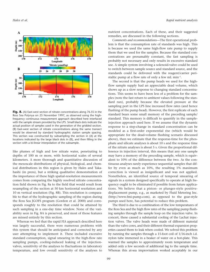
like plumes of high and low nitrate water, penetrating todepths of 100 m or more, with horizontal scales of severalkilometers. A more thorough and quantitative discussion ofthe mesoscale distributions of physical, biological, and chem-ical distributions in this region is given by Hales and Taka-hashi (in press), but a striking qualitative demonstration ofthe importance of these high spatial-resolution measurementscomes from comparing the highly resolved nitrate concentra-tion field shown in Fig. 8a to the field that would result fromresampling of the section at 50 km horizontal resolution and10 m vertical resolution (Fig. 8B). This resolution is compara-ble to that of the hydrographic sampling of the region duringthe Ross Sea JGOFS program (Gordon et al. 2000) and corre-sponds roughly to the resolution that could be attained bysuch sampling in a one-day time window. None of the vari-ability seen in Fig. 8A is preserved, and most of those featuresare missed entirely by this section.

Whereas we feel that the rapid FIA approach described herewas largely successful, there were numerous problems withthis system that should be anticipated and corrected by anyuser attempting to implement it. These included excessivestandard consumption, signal smearing in the high-flow ratesampling pumps, cooling-induced leaking of the injection-valves, sensitivity of the analyses to fluctuations in laboratorytemperature, and low overall sensitivity of the analyses to

nutrient concentrations. Each of these, and their suggestedremedies, are discussed in the following sections.

Comments and recommendations—The first operational prob-lem is that the consumption rate of standards was high. Thisis because we used the same high-flow rate pump to supplythem that we used for the samples. Because the standard con-centrations are presumably constant, the fast sampling isprobably not necessary and only results in excessive standarduse. A simple system involving a solenoid-valve could be usedto switch between sample source and standard source, and thestandards could be delivered with the reagent/carrier peri-staltic pump at a flow rate of only a few mL min–1.

The second is that the pump heads we used for the high-flow sample supply had an appreciable dead volume, whichshows up as a slow response to changing standard concentra-tions. This seems to have been less of a problem for the sam-ples (note the fast return to ambient values following the stan-dard run), probably because the elevated pressure at thesampling port in the LPS line increased flow rates (and henceflushing of the pump head). However, the first replicate of eachstandard bears some small memory of the preceding sample/standard. This memory is difficult to quantify in the sample-injection approach used here. If we assume that the dynamicresponse to a step-change in standard concentration can bemodeled as a first-order exponential rise (which would beappropriate for the dead-volume flushing scenario discussedabove), then we estimate that the response-time for the phos-phate and silicate analyses is about 10 s and the response timeof the nitrate analyses is about 5 s. Given the proportional dif-ference in injection interval, this means that any one samplemay have a memory of the preceding sample, which is equiv-alent to 10% of the difference between the two. As the con-tinuous analyses rarely experience sequential samples that dif-fer by even as much as 10%, the resulting 1% maximumcorrection is viewed as insignificant and was not applied.Nonetheless, an identified source of temporal smearing ofsignals in a system designed specifically to operate at high fre-quency ought to be eliminated if possible from future applica-tions. We believe that a piston- or plunger-style positive-displacement pump, e.g., as marketed by Fluid Metering Inc.(http://www.fmi-pump.com), as opposed to the gear-stylepumps used here, has potential to reduce this problem.

The third is due to a combination of the low temperatures ofthe Ross Sea and the high flow rates of the sampling pump flush-ing samples through the sample loop on the injection valve. Inconcert, these caused a substantial cooling of the Lachat injec-tion valves. The valve heads were made of different materialthan the valve cores, and their different thermal expansion prop-erties caused them to leak when cooled. We solved this problemby running the samples through a 15-foot coil of 1/16-inch i.d.nylon tube immersed in a beaker of water on a hot-plate. Thiswarmed the samples to approximately room temperature andadded only a few seconds of additional lag to the sample time.Whereas this at-sea improvisation worked acceptably in our

Hales et al. Rapid nutrient analysis

99

Fig. 8. (A) East-west section of nitrate concentrations along 76.5S in theRoss Sea Polynya on 25 November 1997, as observed using the high-frequency continuous measurement approach described here interfacedwith the sample stream provided by the LPS. Small black dots indicate theactual position of samples used in the generation of the gridded section.(B) East-west section of nitrate concentrations along the same transectwould be observed by standard hydrographic station sample spacing.This section was constructed by subsampling the section in (A) at thelocations indicated by the large black dots in (B), and then filling in thesection with a bi-linear interpolation of the subsample.

application, there was a delicate balance between the hot-platesetting and the sample flow rate. Setting the hot plate too highwould excessively heat the samples, causing significant out-gassing and bubbling, while setting it too low would insuffi-ciently warm the samples, causing the valves to leak. We suggestthat users working in frigid waters should plan to include a ther-mostated heating system appropriate to the flow rates and tem-peratures of the high-flow sample line.

Fourth, our Si and N chemistry exhibited some sensitivityto the temperature of the laboratory. Granted, we were doingour work in a particularly poor thermal-controlled setting.Our lab space was in an uninsulated room, heated by a singlelarge blower with wide temperature tolerances, and the onlyavailable bench space was situated directly beneath thisblower. Further confounding this issue was the fact that thislab was a major walkway from interior labs to the open deck.Frequent opening and intermittent closing of exterior doorsled to large temperature swings in the laboratory, which werereflected dramatically in the silicate analysis and to someextent in the nitrate analysis. Phosphate, however, showed nosuch sensitivity because of the presence of a heated, ther-mostated block around which the primary reaction coil waswound. One solution is to simply demand better laboratoryconditions; however seagoing analytical chemists can’t alwaysenforce such demands. The best solution is to add heated,thermostated control to both the N and Si reaction columns.

Finally, the combination of small sample loops and shortresidence times in reaction volumes led to greatly limited sen-sitivity. This was not a significant problem in the early-bloomconditions of the Ross Sea where nutrient concentrations werehigh and also highly variable. Potential users should be cau-tious, however, about taking such a system to sea in a settingwhere concentrations and variability are low. Adding the heat-ing elements to the analytical systems, described above, maysignificantly alleviate this problem as heat speeds chemicalreactions and thus reduces the requirement for long reactiontimes. Other solutions, however, such as increasing sampleloop size or increasing reaction residence time, will directlyand negatively impact sampling frequency. This remains anunresolved problem with this approach.

ReferencesAiken, J. 1985. The undulating oceanographic recorder mark

2. A multirole oceanographic sampler for mapping andmodeling the biophysical marine environment. Amer.Chem. Soc. 209:315-332.

———. 1981. The undulating oceanographic recorder mark 2.J. Plankton Res. 3:551-560.

———, R. H. Bruce, and J. A. Lindley. 1977. Ecological investi-gations with the undulating oceanographic recorder: thehydrography and plankton of the waters adjacent to theOrkney and Shetland Islands. Mar. Biol. 39:77-91

Arrigo, K. R., D. H. Robinson, D. L. Worthen, R. B. Dunbar,G. R. DiTullio, M. VanWoert, and M. P. Lizotte. 1999. Phyto-

plankton community structure and the drawdown of nutri-ents and CO2 in the Southern Ocean. Science 283:365-367.

Bahr, F., and P. D. Fucile. 1995. SeaSoar—a flying CTD.Oceanus 38:26-27.

Bates, N. R., D. A. Hansell, C. A. Carlson, and L. I. Gordon.1998. Distribution of CO2 species, estimates of net commu-nity production, and air-sea CO2 exchange in the Ross Seapolynya. J. Geophys. Res. 103:2883-2896.

Bird, R. B., W. E. Stewart, and E. N. Lightfoot. 1960. Chapter 2,p. 34-70. In Transport phenomena. Wiley.

Codispoti, L. A., G. E. Friederich, J. W. Murray, and C. M.Sakamoto. 1991. Chemical variability in the Black Sea:implications of continuous vertical profiles that penetratedthe oxic/anoxic interface. Deep-Sea Res. 38(supp. 2):S691-S710.

Dessureault, J.-G. 1975. Batfish: a depth-controllable towedbody for collecting oceanographic data. Ocean Eng. 3:99-111.

Dugdale, R. C., and F. P. Wilkerson. 1998. Silicate regulation ofnew production in the equatorial Pacific upwelling. Nature393:270-273.

Friederich, G. E., and L. A. Codispoti. 1987. An analysis of con-tinuous vertical nutrient profiles taken during a cold-anomalyoff Peru. Deep-Sea Res. 34:1049-1065.

Gordon, L. I., L. A. Codispoti, J. C. Jennings, F. J. Millero, J. M.Morrison, and C. Sweeney. 2000. Seasonal evolution ofhydrographic properties in the Ross Sea, Antarctica 1996-1997. Deep-Sea Res. II 47:3095-3118.

Grasshoff, M. 1983. Determination of nitrate, p. 143-187. In K.Grasshoff, M. Erhardt, and K. Kremling, Methods of seawa-ter analysis, Verlag Chemie.

———, K. Erhardt, and K. Kremling. 1983. Determination ofnutrients, p. 143-150. In K. Grasshoff, M. Erhardt, and K.Kremling, Methods of seawater analysis, Verlag Chemie.

Griffiths, G., and R. T. Pollard. 1992. Tools for upper ocean sur-veys. Sea Technol. 33:25-32.

Hales, B., and T. Takahashi. 2002. The pumping SeaSoar: ahigh-resolution seawater sampling platform. J. OceanicAtmospheric Technol. 19:1096-1104.

——— and ———. In press. High-resolution biogeochemicalinvestigation of the Ross Sea, Antarctica, during AESOPS(U.S. JGOFS) program. Global Biogeochem. Cycles.

Hermann, A. W., and T. M. Dauphinee. 1980. Continuous andrapid profiling of zooplankton with an electronic countermounted on a ‘Batfish’ vehicle. Deep-Sea Res. 27:79-96.

Johnson, K. M., and R. L. Petty. 1983. Determination of nitrateand nitrite in seawater by flow injection analysis. Limnol.Oceanogr. 28:1260-1266.

Koroleff, F. 1983a. Determination of phosphorus, p. 125-129.In K. Grasshoff, M. Erhardt, and K. Kremling, Methods ofseawater analysis, Verlag Chemie.

———. 1983b. Determination of silicon, p. 174-181. In K.Grasshoff, M. Erhardt, and K. Kremling, Methods of seawa-ter analysis, Verlag Chemie.

Hales et al. Rapid nutrient analysis

100

Nydahl, F. 1976. On the optimum conditions for the reduc-tion of nitrate to nitrite by cadmium. Talanta 23:349-357.

Pollard, R. T. 1986. Frontal surveys with a towed profiling con-ductivity/temperature/depth measurement package (Sea-Soar). Nature 323:433-435.

Rubin, S. I. 2003. Carbon and nutrient cycling in the upperwater column across the polar frontal zone along 170° W.Global Biogeochem. Cycles 17:1087-1102.

Smith, W. O., R. F. Anderson, J. K. Moore, L. A. Codispoti, andJ. M. Morrison, (2000). The US Southern Ocean JointGlobal Ocean Flux Study: an introduction to AESOPS Deep-Sea Res. II 47:3073-3094.

Sweeney, C., W. O. Smith, B. Hales, and others. 2000. Nutrientand carbon removal ratios and fluxes in the Ross Sea,Antarctica. Deep-Sea Res. II 47:3395-3421.

Takeda, S. 1998. Influence of iron availability on nutrient con-sumption ratio of diatoms in oceanic waters. Nature393:774-777.

Tyrell, T. 1999. The relative influences of nitrogen and phos-phorus on oceanic primary production. Nature 400:525-531.

Submitted 17 June 2003

Revised 5 November 2003

Accepted 12 December 2003

Hales et al. Rapid nutrient analysis

101